Mass Residuals as a Criterion for Mesh Refinement in Continuous

Mass Residuals as a Criterion for Mesh Refinementin Continuous Galerkin Shallow Water Models

J. C. Dietrich1; R. L. Kolar, M.ASCE2; and K. M. Dresback3

Abstract: Mass balance error has been computed traditionally by using conventional fluxes derived from the conservation of massequation, but recent literature supports a method based on fluxes that are consistent with the discretization of the governing equations. Bycomparing the mass residuals from these two methods to the truncation errors produced by the discretization of the governing equations,we show that the conventional fluxes produce mass residuals that are more descriptive of the overall behavior of the model, i.e., they arebetter correlated with truncation error. Then we demonstrate that these mass residuals can be used as a criterion for mesh refinement. Inan example using a one-dimensional shallow water model, we demonstrate that, by moving nodes from regions with large mass residualsto regions with small mass residuals, a mesh can be developed that shows less truncation error than a mesh developed by using localizedtruncation error analysis. And, in an example using a two-dimensional shallow water model, we demonstrate that the computed solutioncan be improved in regions with large mass residuals through mesh refinement.

DOI: 10.1061/�ASCE�0733-9429�2008�134:5�520�

CE Database subject headings: Mesh generation; Numerical models; Hydrodynamics; Finite element method; Shallow water.

Background

The use of norms for error diagnosis has a long and diverse his-tory. Gresho and Lee �1981� argued that oscillatory solutions are“good” in that they provide motivation for reexamination ofboundary conditions, geometry, meshing, and problem formula-tion. By examining the errors in a computed solution, it is pos-sible to identify parts of the model that require improvement.Researchers have applied this idea in the areas of mesh generationand refinement. Some researchers refine meshes by examining thesolution or its derivatives �Behrens 1998; Cascon et al. 2003;Marrocu and Ambrosi 1999; Wille 1998�. These adaptive meshingtechniques use a posteriori error estimators that are based on thecomputed response, and they have been applied successfully inshallow water applications. However, because these techniquesare based on solution error, which often involves a discrete esti-mate of the gradient of the computed response, they can reintro-duce truncation error.

Other researchers generate meshes based on a localized trun-cation error analysis �LTEA�, which minimizes phasing and am-

1Graduate Student, Dept. of Civil Engineering and GeologicalSciences, Univ. of Notre Dame, 156 Fitzpatrick Hall, Notre Dame,IN 46556 �corresponding author�. E-mail: [email protected]

2Professor, School of Civil Engineering and Environmental Science,Univ. of Oklahoma, 202 W. Boyd St., Room 334, Norman, OK 73019.E-mail: [email protected]

3Research Associate, School of Civil Engineering and EnvironmentalScience, Univ. of Oklahoma, 202 W. Boyd St., Room 334, Norman,OK 73019. E-mail: [email protected]

Note. Discussion open until October 1, 2008. Separate discussionsmust be submitted for individual papers. To extend the closing date byone month, a written request must be filed with the ASCE ManagingEditor. The manuscript for this paper was submitted for review and pos-sible publication on September 13, 2005; approved on September 14,2007. This paper is part of the Journal of Hydraulic Engineering, Vol.134, No. 5, May 1, 2008. ©ASCE, ISSN 0733-9429/2008/5-520–532/
$25.00.
520 / JOURNAL OF HYDRAULIC ENGINEERING © ASCE / MAY 2008

plitude errors �Hagen et al. 2000, 2001�. In the review of adaptivemesh strategies by Baker �1997�, the author mentions earlier usesof truncation error as a meshing criterion �Berger and Jameson1985; Berger and Oliger 1984; Lee and Tsuei 1993� but notes that“�s�urprisingly, this approach to error estimation does not appearto have gained much acceptance.” One possible reason is that it iscostly to develop these grids because they require a priori calcu-lation of the truncation errors, which require knowledge of the“true” solution, typically obtained from a uniformly and highlyrefined mesh. And, like the adaptive strategies above, these strat-egies require a discrete estimate of derivatives, albeit on a finermesh, so truncation error is minimized.

In this paper, we examine the use of mass residuals as a cri-terion for mesh refinement. Mass conservation must be a con-sideration for any shallow water model, but it is especiallyimportant for continuous Galerkin finite-element models, such asthe advanced circulation �ADCIRC� family of models used in thenumerical examples in this paper �Luettich and Westerink 1992;Luettich and Westerink, unpublished online user’s manual, 2004�.In particular, continuous Galerkin finite-element models can suf-fer from global or local mass error �Lynch 1985�. Global massbalance errors can be eliminated through proper treatment of theboundary conditions �Lynch 1985; Kolar et al. 1996�. However,local mass errors can persist in complex applications, such asregions with rapidly converging/diverging flow or wetting anddrying �Kolar et al. 1994; Horritt 2002�. In addition, local masserrors are acutely problematic when a shallow water model iscoupled to a transport model. If water mass is not conserved, thenthe transport model will show artificial gains or losses in the massof the transported species. Minimization of these local mass re-siduals would improve the behavior of the shallow water model inall of these applications. Furthermore, and in contrast to meshrefinement based on LTEA, mesh refinement based on mass re-siduals does not require knowledge of the forms of the truncationerror terms and does not require a highly resolved backgroundgrid �Hagen et al. 2000, 2001�. Thus, it has the potential to be
performed in real time, to improve resolution in wetting and dry-

ing regions as a storm surge inundates and recedes, for example.We examine this criterion in the framework of two research

questions. First: Which mass residual is a better indicator of trun-cation errors? Second: Can this mass residual be used as a crite-rion for mesh refinement?

Recent literature disagrees about the best method to computelocal mass residuals in models based on the continuous Galerkinfinite-element method; specifically, there is disagreement abouthow best to compute flux. A conventional method of computingflux would begin with the conservation of mass equation andevaluate a boundary integral, which in one dimension gives thefamiliar Q=HU, where Q�flux; H�total water depth; andU�depth-averaged velocity �Kolar et al. 1994�. However, inmodels based on the continuous Galerkin finite-element method,mass conservation is enforced globally. Thus, when the conven-tional fluxes are computed locally in those models, the fluxes maynot necessarily conserve mass because they are not consistentwith the finite-element discretization of the governing equations�Hughes et al. 2000; Berger and Howington 2002�. Instead, it ispossible to derive fluxes that are consistent with the discretizationand that conserve mass locally. In this paper, we derive both theconventional flux and consistent fluxes for the one-dimensionalADCIRC model, and then we examine how well the respectiveresiduals correlate with local truncation errors. If these mass re-siduals do indeed correlate with local truncation errors, then theymight be used as a mesh refinement criterion.

In the sections that follow, we derive the fluxes and theirrespective error norms, examine their correlation with local trun-cation errors in two test cases, and demonstrate the developmentof a computational mesh based on the minimization of massresiduals, both in one and two dimensions. These analyses willbe conducted with the ADCIRC family of models �Kolar andWesterink 2000�, which have found use in a variety of applica-tions, ranging from storm surge calculations to ecosystem studies�Westerink et al. 2008; Luettich et al. 1999�. ADCIRC is based onthe generalized wave continuity �GWC� equation and the continu-ous Galerkin finite-element method. The GWC equation was firstdeveloped by Lynch and Gray �1979� and Kinnmark �1984,1985�, and it employs a numerical parameter G that weights thecontributions of the wave equation and the primitive continuityequation to prevent spurious oscillations. However, ADCIRC’simplementation of the GWC equation is not dissimilar from shal-low water models based on the continuity equation; for example,if the numerical parameter G is selected carefully, then the dis-cretization of the GWC equation can be shown to be equivalent tothe discretization of the continuity equation using the quasi-bubble scheme employed by Telemac �Mewis and Holtz 1993;Atkinson et al. 2004�. Furthermore, the results herein can be ap-plied to other shallow water models, such as Norton et al. �1973�or Lynch et al. �1996�, which are based on the continuous Galer-kin finite-element method. In any model that does not enforcemass conservation locally, the mass residuals might be useful as acriterion for mesh refinement.

Methods

Mass Residuals

The algorithm to evaluate mass conservation was presented by
one of the writers in a previous work �Kolar et al. 1994�; it is
J

repeated here for completeness. The conservation of mass equa-tion reduces to the depth-averaged continuity equation under shal-low water assumptions, to get

��

�t+ � · �HU� = 0 �1�

where ��departure of the water surface elevation from the mean;��gradient operator in two dimensions; H�total water depth;and U�depth-averaged velocity. Integrate Eq. �1� over space andtime to obtain

�t0

t ��

� ��

�t+ � · �HU��d� dt = 0 �2�

where ��entire domain �for a global check of mass conserva-tion� or one element or a patch of elements �for a local check ofmass conservation�; t�time; and t0�reference time, such as thebeginning of the simulation. The first term in Eq. �2� is integratedover time and the divergence theorem is applied to the secondterm to obtain

��

��t − �0�d� +�t0

t ��

HU · n d��dt = 0 �3�

where the first term represents accumulation and the second termrepresents net flux. Now we approximate the dependent variableswith their discrete counterparts. For the first term in Eq. �3�, weapproximate � with linear Lagrange basis functions and evaluateexactly the integral as

��

��t − �0�d� = �e

��t − �t0�eAe �4�

where Ae�area of element e; �̄�arithmetic average of the nodalvalues of � over the element; and the sum is over all elements inthe domain of interest.

For the second term in Eq. �3�, the boundary integral repre-sents the net flux into the domain, where n�unit outward normalvector. There is disagreement in the literature about the bestmethod to compute this net flux. For now, we define

Qnet =��

HU · n d�� 5�

and then we approximate the second term in Eq. �3� using thetrapezoidal rule

�t0

t ��

HU · n d��dt =�t0

t

Qnet dt �k

1

2�Qnet

t+�t + Qnett ��t

�6�

where k�time step index. Note that, in order to keep the deriva-tion more general, the above relations were derived for a two-dimensional model; they can be simplified easily to theirone-dimensional counterparts. In the ensuing derivation, the pointof departure will be the one-dimensional equations in order tokeep the mathematics tractable.

Thus, for a single one-dimensional element to conserve masslocally over one time step, it would have to satisfy exactly thisequation

��t+�t − �t��xe + 12 �Qnet

t+�t + Qnett ��t = 0 �7�

where �xe�length of the element. If any residual error exists,
then it would appear as a nonzero sum.
OURNAL OF HYDRAULIC ENGINEERING © ASCE / MAY 2008 / 521

Debate in the literature centers around how to evaluate the netflux, Qnet, defined in Eq. �5�. We examine two methods of com-puting fluxes. The first method evaluates the boundary integral inEq. �5� using exact quadrature. Thus, in one dimension, the inte-gral reduces to point evaluations of H and U at the boundaries ofthe element

Qnet,V ��

HU · nd�� = − HLUL + HRUR �8�

where the subscripts L and R denote left and right boundaries ofa one-dimensional element, respectively; and the subscript V in-dicates that these fluxes are denoted as conventional fluxes. Be-cause it is based on the continuous Galerkin method and theGWC equation, the ADCIRC model does not enforce locally themass conservation equation shown in Eq. �1�. Our first error mea-sure uses Eq. �7� and the conventional fluxes from Eq. �8� toobtain

�V = ��t+�t − �t��xe + 12 �Qnet,V

t+�t + Qnet,Vt ��t� �9�

where �V�mass balance residual. This residual is not normalizedto the still water volume in the element or the departure from thestill water volume in the element. We examine only the magni-tudes of these residuals for ease of comparison with the localtruncation errors, for reasons explained below.

The second method solves for fluxes in a manner that isconsistent with the Galerkin finite-element formulation of theGWC equation. According to Hughes et al. �2000� and Berger andHowington �2002�, fluxes computed in this manner are locallyconservative. A comprehensive derivation of these fluxes for theone-dimensional ADCIRC model can be found in Dietrich et al.�unpublished internal report, 2006�; we include the significantsteps here. Begin with the one-dimensional form of the GWCequation

�2�

�t2 + G��

�t− HU

�G

�x

−�

�x� �

�x�HUU� + gH

��

�x− El

�2

�x2 �HU� + �HU − GHU� = 0

�10�

where G�numerical parameter introduced by Kinnmark �1985,1986�; g�gravitational constant; El�lateral eddy viscosity; and��bottom friction parameter, here assumed to be a constant andto have units of sec−1. Note that, for all of the test cases herein,the eddy viscosity has been assumed to be constant. For con-venience, we replace the quantity in brackets with the dummyvariable A, multiply by the linear Lagrange weight function asso-ciated with node i, and integrate over two elements containingnode i to obtain

�xi−1

xi � �2�

�t2 + G��

�t− HU

�G

�x−

�A

�x �i dx

+�xi

xi+1 � �2�

�t2 + G��

�t− HU

�G

�x−

�A

�x �i dx = 0 �11�

Apply integration by parts to the last term in both integrals to
obtain

�xi−1

xi �� 2�

�t2 + G��

�t− HU

�G

�x �i + A

d�i

dx�dx − �A�i��xi

−

+�xi

xi+1 �� 2�

�t2 + G��

�t− HU

�G

�x �i + A

d�i

dx�dx + �A�i��xi

+ = 0

�12�

where we have utilized �i�xi−1�=0 and �i�xi+1�=0. In the twoboundary terms, the superscripts indicate contributions from theleft �−� or right �+� of the node. By substituting the one-dimensional forms of the conservation equations for mass andmomentum, we can simplify the dummy variable A in thoseboundary terms to

�xi−1

xi �� 2�

�t2 + G��

�t− HU

�G

�x �i + A

d�i

dx�dx

+ �� Q

�t+ GQ �i��

xi−

+�xi

xi+1 �� 2�

�t2 + G��

�t− HU

�G

�x �i + A

d�i

dx�dx

− �� Q

�t+ GQ �i��

xi+

= 0 �13�

where Q�flux through node i. In an example by Berger andHowington �2002� of the advective transport of a conservativetracer, only the flux Q appears in the boundary terms, and thusthey are able to solve for fluxes that are both locally conservativeand continuous at the nodes. However, the GWC equation is aderivative form of the shallow water equations, which gives riseto the �Q /�t+GQ term on the boundary. Thus, we are unable toenforce continuity of flux directly at each node; rather, we enforcecontinuity of the quantity �Q /�t+GQ. To do so, we require

�� Q

�t+ GQ �

xi−

= −�xi−1

xi � �2�

�t2 �i + G��

�t�i − HU

�G

�x�i + A

d�i

dx dx �14�

and

�� Q

�t+ GQ �

xi+

=�xi

xi+1 � �2�

�t2 �i + G��

�t�i − HU

�G

�x�i + A

d�i

dx dx

�15�

Eqs. �14� and �15� can be thought of as ordinary differential equa-tions that can be solved for Q, in a manner similar to Massey andBlain �2006�. It should be noted that the resulting discrete fluxequations are quite complex, involving many terms, and thus it isnot possible to attach the same physical interpretation that wasdone for the conventional fluxes shown in Eq. �8�. However, inthe limit as G→�, the fluxes at the boundary can be recovered interms of just Q.

Using these consistent fluxes, we can solve for the net flux inan element

Qnet,S = − QL + QR = − Qxi+ + Qxi+1

− �16�

where the flux Qxi+ corresponds to the right side of node i, and the

−
flux Qxi+1corresponds to the left side of node i+1. �The flux is

continuous across node i only if Qxi+ =Qxi+1

− �. Then define a seconderror measure

�S = ��t+�t − �t��xe + 12 �Qnet,S

t+�t + Qnet,St ��t� �17�

where �S�mass balance residual when the net fluxes Qnet,S areevaluated using the consistent flux statement given in Eq. �16�.�Note that we are using the subscript V to denote conVentionaland the subscript S to denote conSistent.�

Note that the error norms defined in Eqs. �9� and �17� aredimensional. They could be normalized to the deviation from thestill water volume of the element by dividing by �t+�t�xe, where�t+�t��L,t+�t+�R,t+�t� /2�average at time t+�t of the water sur-face elevation departures from the mean for the nodes on the left�L� and right �R� of a one-dimensional element, and �xe�lengthof that element. However, this normalization is counterproductivein the framework of this work, where the goal is to establish amass residual that can be used as a criterion for mesh refinement.If the error norm is related inversely to the mesh spacing, i.e., ifdecreases in the mass residual in the numerator are offset bydecreases in the mesh spacing in the denominator, then the errornorm may not converge as the mesh is refined. In fact, in ourexperience, the normalized mass residuals have sometimes in-creased as the mesh is refined, which is not the case for theresiduals as they are defined above. In short, normalization of theresiduals masks the actual error in the domain and limits inter-mesh comparisons. For those reasons, we use the non-normalizedresiduals herein.

We stress the importance of the flux discontinuities at thenodes. This result is a significant departure from the results pre-sented by Berger and Howington �2002�, and it calls into questionthe utility of the consistent flux approach. Mass conservation isnecessary in transport applications, but those applications requirea continuous flux in order to conserve information from one ele-ment to the next. Without a continuous flux, the perfect elementalmass conservation given by the consistent fluxes is lost. In orderto examine this behavior in the context of the GWC equation withrespect to local truncation errors and mesh refinement, we definethe discontinuity

S = �Qxi+ − Qxi

−� �18�

which becomes our third error norm. In contrast to the massbalance residuals defined in Eqs. �9� and �17�, the discontinuitydefined in Eq. �18� is nodal based.

Truncation Errors

ADCIRC is based on two equations: the GWC equation, which isa derivative form of the mass conservation equation; and the non-conservative form of the momentum equation �NCM�. The GWCequation is shown in Eq. �10�. The NCM equation in one dimen-sion is

�U

�t+ U

�U

�x+ �U + g

��

�x−

El

H

�2

�x2 �HU� = 0 �19�

where the variables are defined previously. In the one-dimensional form of the ADCIRC model, the GWC andNCM equations are discretized using linear Lagrange basisfunctions and a Galerkin finite-element scheme in space, aCrank–Nicolson scheme on the linear terms in time, and an ex-plicit formulation for the nonlinear terms in time. We utilize exactquadrature rules and an L2 interpolation for the advective terms.
Full details for the higher-dimensional forms of ADCIRC can be
J

found in Luettich and Westerink �unpublished online user’smanual, 2004�.

Truncation error expressions for every term in the equationswere developed by expanding in a Taylor series about a com-mon interior node point. Use of a symbolic manipulator, such asMathematica, allows us to carry out the analysis with confidenceup to any order for the full nonlinear equations �which requireproducts of Taylor series�. These truncation error expressions canbe found in Dresback and Kolar �unpublished internal report,2004� or in Dresback �2005�. A qualitative examination of theseexpressions shows that the GWC and NCM equations are first-order accurate in time, first-order accurate in space for variablenode spacing, and second-order accurate in space for constantnode spacing. The NCM equation becomes second-order accuratein time if the equation is linearized.

A quantitative examination of the truncation error expressionsrequires information from both fine and coarse grid solutions. Forexample, the first term in the GWC equation is the time derivativeterm, �2� /�t2. In its truncation error expression, the leading orderterm is second order in time and is given by

1

36��xj − �xj−1��t�2 �5� j,k

�x � t4 �20�

where j�spatial index; and k�temporal index. To approximatethe derivatives that appear in the truncation error expressions, weuse second-order central difference schemes on a fine grid �true�solution, which is obtained by refining the grid until the solutionconverges to the sixth decimal place. To evaluate the rest of theterms in the expressions, such as the nonderivative components inEq. �20�, we use information from a coarse grid solution, namely,a coarse grid spacing, time step, and parameter values. The trun-cation errors for all terms in the GWC and NCM equations aresummed and compared against the mass residuals �V and �S andthe flux discontinuity S, as computed from the coarse grid simu-lation. Note that we examine the magnitudes of these truncationerrors, to prevent cancellation of errors due to opposite signs.

For the ensuing discussion, it is useful to think of the trunca-tion error expression in Eq. �20� as containing a derivative partand a grid/parameter part. For all of the truncation error terms, thederivative part is independent of the coarse grid discretization andthus fixed �for a given domain and a given simulation�. And it isevaluated by using a true solution, which in our case is a fine gridsolution that remains the same for all coarse discretizations. Re-gardless of the coarse grid that is used to discretize this domain,these values from the derivative parts of the errors will persist.However, because the algorithm is consistent, the product of thegrid/parameter and derivative parts goes to zero in the limit as thegrid is refined.

On the other hand, the grid/parameter component of each trun-cation error term is dependent on the discretization and otheruser-selected parameters. A modeler can manipulate this compo-nent to alter algorithm behavior. In fact, some grids are designedto minimize the coarse component in regions where the fine com-ponent is large �and vice versa�, so that the overall truncationerror is uniform throughout the computational domain �Hagenet al. 2000, 2001�.

Analyses in One Dimension

We examine initially the relationships between our error norms
and local truncation errors using a one-dimensional test based on

a slice of an ocean shelf and basin �shown in Fig. 1�; we will referto it as the shelf break domain. It is an idealized version of theWestern North Atlantic Ocean, as if a slice had been taken per-pendicular to the United States coastline and extended into thedeep ocean �Hagen et al. 2000�. Local mass errors have beenobserved to occur in regions with rapidly changing bathymetrywhere the flow converges or diverges �Kolar et al. 1994�. Thisdomain contains a shelf break where the bathymetry increasesrapidly from a depth of 200 m to a depth of 5 km, and thus itshould be a good test of the model’s local mass conservation andtruncation error properties.

The first test on this domain has a constant grid spacing ofabout 44.4 km, which corresponds to 46 nodes. The second teston this domain has the same number of nodes, but they are vari-ably spaced, as determined from the LTEA method �Hagen et al.2000, 2001�. The LTEA method places nodes based on the trun-cation errors associated with the discrete form of the linearized,harmonic conservation of momentum equation, and it has beenshown to improve both accuracy and efficiency. The grid spacingranges from about 112.5 km in the deep water to 1 km at the shelfbreak. Fig. 2 compares the two different node placements for theshelf break domain. Note that the LTEA method clusters nodes ata distance into the domain of about 1,750 km, which is where thebreak in the bathymetry occurs.

Both meshes share the following simulation parameters: a timestep of 1 s, a simulation time of 3.24 M2 tidal cycles �or 40.24 h�,a constant bottom friction of 0.0001 s−1, a lateral eddy viscosityof zero, and a numerical G parameter of 0.001 s−1. They also

Fig. 1. Bathymetry for shelf break domain �adapted from Hagenet al. 2000�

Fig. 2. Distribution of nodes for last 400 km of shelf break domain,for three meshes


share the same fine grid �“true”� solution, which utilizes 8,193nodes and a constant grid spacing of 244 m. This fine grid wasobtained by refining the shelf break �constant spacing� domainuntil the solution converged to the sixth decimal place. We willpresent errors from the third to last time step in these simulations,so the elevation and velocity output from the fine grid solutionwas saved for the last five time steps and used to estimate thederivatives in the truncation error terms.

Shelf Break Domain—Constant Spacing

The constant spacing version of the shelf break domain is aninteresting test of both mass residuals and local truncation errors,because no attempt has been made to place nodes in a manner thatminimizes error. The mass residuals �V �which uses the conven-tional flux� and �S �which uses the consistent fluxes� are shown asthe solid lines in Figs. 3 and 4, respectively. The mass residual�V is relatively small throughout most of the domain, except forthe shelf break region, where the residual reaches a maximummagnitude of 29.9 m2. �The normalized residuals, which we men-tion only as a means of comparison, would be in the range of10−6–10−3% of the deviation from the still water volume through-out most of the domain, and 0.6% of the deviation from the stillwater volume in the shelf break region.� In contrast, the massresidual �S shows a steady increase throughout the domain, andits maximum magnitude of 1.6·10−6 m2 occurs at the land bound-

Fig. 3. Mass residuals �V for one-dimensional domains. Shelf break�constant spacing� residuals are shown in solid line, shelf break�LTEA� residuals are shown in dashed line, and shelf break �concept�residuals are shown in dotted line.

Fig. 4. Mass residuals �S for one-dimensional domains. Shelf break�constant spacing� residuals are shown in solid line, and shelf break�LTEA� residuals are shown in dashed line.

ary on the right side of the domain. The third error norm, theconsistent flux discontinuity S, is shown as a solid line in Fig. 5.The discontinuities increase throughout the domain, but there is anoticeable change in their behavior at the shelf break, where thediscontinuities oscillate with a wavelength of 2�x.

We offer two observations based on the error norms them-selves. First, the mass residuals based on the conventional fluxesare significantly larger than the mass residuals based on the con-sistent fluxes. This behavior is to be expected, because the con-sistent fluxes are derived in a manner that is consistent with thediscretization of the governing equations, and they are evaluatedusing computed solutions for that element. However, because ofthe problems described above regarding the derivation of the con-sistent fluxes for the GWC equation, the mass residual �S basedon these fluxes does not perfectly conserve mass on the elementlevel. Although the errors shown as the dashed line in Fig. 4 aresmall, they are too large to be round-off error. Second, only themass residual �V has its maximum at the shelf break, which islocated at a distance of about 1,780 km into the domain. In con-trast, the mass residual based on the consistent fluxes shows anobvious change in behavior at the shelf break, but its magnitudecontinues to increase on the shelf. The flux discontinuities S alsocontinue to increase on the shelf, and they show a 2�x oscillationthat is not seen in either of the other mass residual plots.

A summary of the truncation errors is shown in Table 1, andthe spatial distribution of the truncation errors for all terms in theGWC and NCM equations are shown as solid lines in Figs. 6 and7, respectively. The maximum truncation error for the GWCequation is 4.27·10−3 m /s2, and the maximum truncation errorfor the NCM equation is 2.07·10−3 m /s2. Table 1 also shows thecorrelations between the truncation errors associated with theterms in the governing equations and the mass and flux errorsassociated with the three norms �V, �S, and S. To perform thiscorrelation, we computed Pearson’s product-moment correlationcoefficient, r, using the local truncation errors and each of themass error norms; the correlation coefficients are shown in thelast three columns of Table 1. Pearson’s product-moment correla-tion coefficient is given by

r12 =� �Yi1 − Y1��Yi2 − Y2�

�� Yi1 − Y1�2 � �Yi2 − Y2�2�21�

where Y1 and Y2�data sets and the overbar indicates a mean

Fig. 5. Consistent flux discontinuities S for one-dimensionaldomains. Shelf break �constant spacing� discontinuities are shown insolid line, and shelf break �LTEA� residuals are shown in dashed line.

�Neter et al. 1996�. The local truncation errors and the consistent

J

flux discontinuities S are node-based errors, whereas the massresiduals �V and �S are element based; to compute the correlationcoefficient, we projected the mass residuals to the nodes by se-lecting the larger of the residuals from the two adjoining ele-ments. This correlation coefficient can range between −1 and 1;for the purposes of mesh refinement, a coefficient of −1 might bejust as useful as a coefficient of 1, because it would still representa strong �albeit negative� correlation between truncation errorsand mass errors. As shown in Table 1, the magnitudes of thecorrelation coefficients for the shelf break �constant spacing� do-main are about 0.5 or less. However, it should be noted that thecoefficients for �V are about 2–3 times larger than the coefficientsfor �S and S, indicating that the conventional fluxes producemass residuals that are a much more useful predictor of truncationerror in the model.

The final study in this section is convergence. As noted above,the local truncation errors for the GWC and NCM equations areformally second-order accurate in space, for constant-spacing do-mains. Recent studies, such as Dawson et al. �2006�, indicate thatsecond-order convergence rates can be observed in both the el-evation and velocity solutions of GWCE-based models, undercertain conditions involving the treatment of the boundary terms,the discretizations of the terms in the governing equations, andthe design of the mesh. A similar convergence study for the shelfbreak �constant spacing� grid was conducted, in which the grid

Fig. 6. Absolute values of truncation errors for all of terms in GWCequation, for one-dimensional domains. Shelf break �constantspacing� errors are shown in solid line, the shelf break �LTEA� errorsare shown in dashed line, and shelf break �concept� errors are shownin dotted line.

Fig. 7. Absolute values of truncation errors for all of terms inNCM equation, for one-dimensional domains. Shelf break �constantspacing� errors are shown in solid line, shelf break �LTEA� errors areshown in dashed line, and shelf break �concept� errors are shown indotted line.


spacing was decreased systematically from 44.4 km to the mini-mum of 244 m used in our fine �“true”� solution. This corre-sponds to an increase in the number of nodes from 46 to 8,193.Each grid spacing corresponds to a unique mesh; the root-mean-square �RMS� errors for elevation and velocity �which are globalerror metrics� were computed for each mesh by comparing thecoarse solution to the “true” solution at the third-to-last time step.The convergence rates for elevation and velocity �not showngraphically herein� were found to be 1.75 and 1.13, respectively.The degradation of the convergence rates from the theoreticalsecond-order rate, especially with respect to velocity, can be at-tributed to several factors, including the implementation of theboundary conditions and the nonlinear behavior in the shelf breakregion. For the velocity solution, the convergence rates at specificnodes in the domain �not shown graphically herein� are consis-tently second order, except in the shelf break region, where theconvergence rates deteriorate to first order. This degradation ofsolution accuracy in the shelf break region limits the convergencerate of the global RMS error.

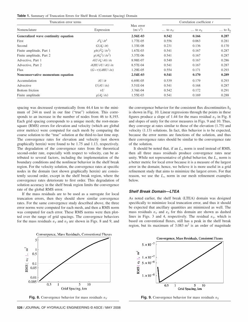
If the mass residuals are to be used as a surrogate for localtruncation errors, then they should show similar convergencerates. For the same convergence study described above, the threeerror norms were computed for each mesh, and then a RMS normwas computed for each error. These RMS norms were then plot-ted over the range of grid spacings. The convergence behaviorsfor the mass residuals �V and �S are shown in Figs. 8 and 9, and

Table 1. Summary of Truncation Errors for Shelf Break �Constant Spac

Truncation error terms

Nomenclature Expression

Generalized wave continuity equationFirst �2� /�t2

Second G�� /�t�Finite amplitude, Part 1 gh��2� /�x2�Finite amplitude, Part 2 g��2� /�x2�Advective, Part 1 ��U�� /�t� /�x

Advective, Part 2 ��HU�U /�t� /�x

Flux �G−��HU /�x�Nonconservative momentum equation

Accumulation �U /�t

Advective U��U /�x�Bottom friction �U

Finite amplitude g�� /�x�

Fig. 8. Convergence behavior for mass residuals �V


the convergence behavior for the consistent flux discontinuities S

is shown in Fig. 10. Linear regressions through the points in thesefigures produce a slope of 1.44 for the mass residual �V in Fig. 8and slopes of unity for the error measures in Figs. 9 and 10. Thus,they converge at rates similar to those of the elevation �1.75� andvelocity �1.13� solutions. In fact, this behavior is to be expected,because the error norms are functions of the solution, and thustheir convergence rates should be similar to the convergence rateof the solution.

It should be noted that, if an L� norm is used instead of RMS,then all three mass residuals produce convergence rates nearunity. While not representative of global behavior, the L� norm isa better metric for local error because it is a measure of the largesterror in the domain; hence, we believe it is more useful in a gridrefinement study that aims to minimize the largest errors. For thatreason, we use the L� norm in our mesh refinement examplesbelow.

Shelf Break Domain—LTEA

As noted earlier, the shelf break �LTEA� domain was designedspecifically to minimize local truncation error, and thus it shouldbe expected that ancillary quantities are minimized as well. Themass residuals �V and �S for this domain are shown as dashedlines in Figs. 3 and 4, respectively. The residual �V, which isbased on conventional fluxes, still has a peak in the shelf breakregion, but its maximum of 3.083 m2 is an order of magnitude

omain

Max error�m /s2�

Correlation coefficient r

… to �V … to �S … to S

2.56E-03 0.542 0.166 0.2871.77E-05 0.556 0.063 0.281

1.33E-08 0.231 0.136 0.170

1.67E-03 0.541 0.167 0.287

3.37E-06 0.541 0.167 0.287

8.98E-07 0.540 0.167 0.286

8.57E-04 0.541 0.167 0.287

1.29E-05 0.554 0.171 0.293

2.54E-03 0.541 0.170 0.289

6.69E-05 0.539 0.179 0.293

5.51E-04 0.541 0.168 0.287

3.76E-04 0.542 0.172 0.291

1.55E-03 0.541 0.169 0.288

Fig. 9. Convergence behavior for mass residuals �S

ing� D

less than the maximum error in the shelf break �constant spacing�domain �shown as the solid line in Fig. 3� and on the same orderof magnitude as the other errors in the domain. The residual �S,which is based on the consistent fluxes, now shows uniform errorsthroughout the domain. Its qualitative behavior again matchesclosely that of the consistent flux discontinuity S, which is shownas a dashed line in Fig. 5.

The truncation errors for the shelf break �LTEA� domain aresummarized in Table 2, and the errors for the GWC and NCMequations are shown as dashed lines in Figs. 6 and 7, respectively.The LTEA method has its intended effect on the truncation errors;the maximum error for the GWC equation decreased by abouttwo orders of magnitude, and the maximum error for the NCMequation decreased by more than one order of magnitude. In bothcases, the peak at the shelf break still exists, but it is both smallerand narrower. A decrease in the error norm based on the conven-tional fluxes corresponds to a similar or larger decrease in thetruncation errors. A qualitative comparison of the mass and trun-cation errors would suggest that the mass residual �V �the dashedline in Fig. 3� correlates to the NCM truncation errors �the dashedline in Fig. 7�, because both show a significant peak at the shelfbreak, and that the mass residual �S �the dashed line in Fig. 4�correlates to the GWC truncation errors �the dashed line in Fig.6�, because both show uniform errors throughout the domain. Thequantitative comparison in Table 2 lends support to this observa-tion, although the correlations are relatively weak, and there is

Table 2. Summary of Truncation Errors for Shelf Break �LTEA� Domai










Fig. 10. Convergence behavior for mass residuals S

J

variability in the correlations on a term-by-term basis in bothequations. More importantly, the LTEA method has succeeded inminimizing the maximum errors and distributing mass and trun-cation errors over the domain, and thus the correlation is notnearly as significant or uniform as it was in the shelf break �con-stant spacing� domain.

Summary

The results of our analyses in one dimension indicate that theconventional fluxes produce mass residuals, �V, that are morestrongly correlated with truncation errors. From the analysis withthe shelf break �constant spacing� domain, we saw that: �1� themass residuals were larger in magnitude, which supports the ex-pectations produced during the derivation; �2� these residualshave their maximum at the shelf break itself, which is also wherethe truncation errors peak; and �3� this relationship can be quan-tified, as the correlation coefficients between the mass residualsand the truncation errors are two to three times larger than corre-lations using other error measures.

Examples of Mesh Refinement Using MassResiduals

It remains to be seen whether these mass residuals can be used asa practical error metric for mesh refinement. In this section, wepresent two examples of mesh refinement using the mass residu-als, �V, based on the conventional fluxes. In the first example, webegin with the shelf break �constant spacing� domain and movenodes until the maximum mass residual is less than the corre-sponding maximum mass residual from the shelf break �LTEA�domain. In the second example, we begin with an irregular, two-dimensional mesh of the Bight of Abaco domain and add nodesuntil the maximum mass residual is less than a prescribed value.

Mesh Refinement in One Dimension

In this section, we demonstrate the development of a grid thatuses mass residuals as the criterion for mesh refinement. We beginwith the shelf break �constant spacing� domain described above,and we make the following assumptions:




8.58E-05 −0.080 0.285 0.4496.10E-05 −0.139 0.442 0.581

3.87E-08 −0.245 0.584 0.719

3.43E-05 −0.030 0.118 0.263

8.08E-08 0.085 −0.222 −0.133

1.20E-07 0.072 −0.170 −0.026

1.69E-05 0.101 −0.266 −0.180

4.75E-06 0.152 −0.231 −0.219

1.67E-04 0.074 −0.176 −0.057

2.95E-06 −0.166 0.473 0.592

7.27E-05 0.078 −0.189 −0.077

2.15E-06 0.135 −0.316 −0.224

9.16E-05 0.079 −0.191 −0.074

n


1. The criterion should be the mass residual �V, which is basedon the conventional fluxes, because we have shown that thisresidual is a better indicator of truncation errors than theerror norms �S and S, which are based on the consistentfluxes;

2. The total number of nodes should remain constant. In otherwords, in order to place a node in a region with large massresiduals, a node must first be removed from a region withsmall mass residuals. The shelf break �constant spacing� do-main has 46 nodes;

3. The removal of a node in a region with low mass balanceerrors should not affect the neighboring nodes. Thus, when anode is removed, its neighbors should not be moved to com-pensate. In effect, the grid spacing in that region is doubled,and it can be increased further during successive iterations;

4. When a node is added to a region with high mass balanceerrors, it should be placed at the midpoint of an existingelement. In effect, the grid spacing in that region is halved;and

5. When a node is added, its bathymetry should be computedfrom a linear interpolation of the surrounding bathymetries.In an automated mesh-refinement scheme, a background gridand higher order interpolation could be used to computebathymetries. However, this is not a concern in this example,because the shelf break �constant� domain uses linear seg-ments of bathymetry, as shown in Fig. 1.

These assumptions were made as much for convenience as forscientific correctness. �It should be noted that some of theseassumptions, such as the effective “doubling” of grid spacingwhen a node is removed, do not have convenient analogues intwo dimensions.� Nonetheless, they allow for a grid develop-ment scenario that illustrates how mass residuals can be used togenerate a mesh that minimizes truncation errors. And, by keep-ing the number of nodes constant, we can compare our conceptmesh to the LTEA mesh with 46 nodes. Future work wouldautomate this procedure; for now, the mesh is refined iteratively,by moving five nodes at a time and then generating an updatedsolution.

We begin with the mass residuals �V based on the conventionalfluxes shown in Fig. 3. For the shelf break �constant spacing�domain, the largest magnitude error is about 29.9 m2, and it oc-curs at a distance of about 1,780 km, which is near where the

Table 3. Summary of Truncation Errors for Shelf Break �Concept� Dom










continental shelf begins its steep descent, as shown in Fig. 1. All


of the significant mass residuals occur in this region. Thus, tominimize these mass residuals, we remove nodes from the deeperparts of the domain and add them to the shelf-break region. Afterfour iterations, in which we move five nodes at a time and recom-pute the mass residuals, we obtain the node placement depicted atthe bottom of Fig. 2.

We can make several observations based solely on the nodedistribution. First, in order to minimize the mass residuals �V, themajority of the nodes were placed in the region where the shelfbegins its steep descent �at a distance of about 1,800 km�. Thegrid spacing in this region is about 2,700 m, or 16 times smallerthan the original constant node spacing. Second, to effect thisdecrease in the node spacing along the shelf break, we removednodes from the deep water portion of the domain. The grid spac-ing in the deep water portion was increased to as high as177,000 m, or four times larger than the original grid spacing.Third, after four iterations, a total of 20 nodes were moved duringthe mesh development.

The effect of this mesh on simulation results is dramatic. Themass residuals �V are shown as a dotted line in Fig. 3. Addingnodes at the shelf break decreases the mass residuals in thatregion, and removing nodes from the deep water increases themass residuals in that region �compared to the results from theregular mesh shown as the solid line in Fig. 3�. The end result isa domain that has a more uniform distribution of error. Note thatthe largest magnitude residual is 5.53 m2, which is a decrease ofabout 81% from the maximum residual produced by the original,constant-spacing mesh. Further iteration on node placement,using a more sophisticated method that placed nodes at locationsother than the midpoint of elements and that limited the relativechange of adjacent elements, would further decrease these massresiduals.

Similar behavior is observed with respect to truncation errors.The dotted line in Fig. 6 shows the truncation errors for all of theterms in the GWC equation, and the dotted line in Fig. 7 showsthe truncation errors for all of the terms in the NCM equation.Note that, although both figures depict peaks at the shelf break,there are nontrivial truncation errors in the deep water region ofthe domain. Qualitatively, the truncation errors match well themass residuals �V; i.e., they are distributed throughout thedomain.

It is important to examine the effect of this mesh refinement in




1.24E-04 0.403 0.166 −0.2035.27E-05 0.248 0.085 −0.441

6.25E-08 0.316 −0.043 −0.722

8.15E-05 0.377 0.159 −0.050

1.93E-07 0.299 0.141 0.097

1.65E-08 0.325 −0.012 −0.515

4.12E-05 0.295 0.141 0.108

1.13E-06 0.317 0.142 0.077

2.11E-05 0.449 0.138 −0.649

1.08E-05 0.433 0.090 −0.679

2.52E-06 0.400 0.186 −0.166

4.73E-06 0.175 0.067 −0.441

9.47E-06 0.351 0.134 −0.486

ain

comparison to the original shelf break �constant spacing� domain

and to the shelf break �LTEA� domain, which was developed byminimizing local truncation error of the linearized, harmonic mo-mentum equation. Table 3 summarizes the truncation errors forthe shelf break �concept� domain. Note that the truncation errorsfrom the concept domain are considerably smaller than those forthe constant-spacing domain. An 81% decrease in the maximummass residual �V created a decrease of one order of magnitude inthe maximum truncation error for the GWC equation and a de-

Fig. 11. Bathymetry of Bight of Abaco, Bahamas, domain with tida

Fig. 12. Meshes of refinement study: �a� initial coars

J

crease of two orders of magnitude in the maximum truncationerror for the NCM equation. Also note that the truncation errorsfrom the concept domain are comparable to those from the LTEAdomain; in fact, the NCM truncation errors are smaller in theconcept domain. �This behavior is most likely due to the fact thatHagen et al. �2000, 2001� used the linear harmonic form of theNCM equation to develop the shelf break �LTEA� domain,whereas this study uses the full, nonlinear, transient form of the

rding stations indicated in figure �adapted from Grenier et al. 1995�

of 926 nodes; �b� final refined mesh of 1,178 nodes

l reco

e mesh


NCM equation.� Thus, not only does this method of mesh refine-ment decrease the truncation errors, it does so as effectively as agrid that was developed by explicitly minimizing truncationerrors.

It should be noted that the correlation coefficients for �V andthe shelf break �concept� domain in Table 3 are significantly bet-ter than the respective correlation coefficients for the shelf break�LTEA� domain in Table 2. Even after we moved 20 nodes andproduced a nonuniform mesh that minimizes both mass residualsand truncation error, the correlations are still 0.403 for the GWCequation and 0.449 for the NCM equation. The respective corre-lations for the shelf break �LTEA� domain are −0.080 and 0.074.Thus, even at this stage in the mesh refinement process, the massresidual �V can still be used as a criterion for further refinement;its utility is not lost.

In summary, by beginning with a mesh that had a constantnode spacing and then moving nodes to minimize the mass re-sidual �V based on the conventional fluxes, we developed a meshthat decreased the maximum mass residual by 81% and decreasedthe maximum truncation errors by one or two orders of magni-tude. In effect, we replicated the positive qualities of the shelfbreak �LTEA� domain without having to compute any truncationerrors during the refinement of the mesh.

Mesh Refinement in Two Dimensions

In this section, we test the concept of using elemental mass re-siduals as a criterion for mesh refinement in a two-dimensionalsetting. In particular, we examine the Bight of Abaco, Bahamas

Fig. 13. Velocity station graphs for Stations 1 and 2, whose locationand �D� show y component of velocity. Dashed line shows results froshows results from “true” solution.

domain; Fig. 11 shows the bathymetry of the area. Land bound-


aries, consisting of the islands around the bight, are treated asno flow boundaries, while the ocean boundary between the is-lands of Abaco and Grand Bahama along the southwest edge ofthe domain is forced with five tidal constituents: O1, K1, N2, M2,and S2. The coarse mesh for this domain consists of 1,696 non-uniform elements and 926 nodes, as shown in Fig. 12�A�. Otherparameters for the simulation are as follows: bottom frictionfactor in the Chezy formulation of 0.009, lateral eddy viscosityof zero, numerical G parameter of 0.009 s−1, time step of 10 s,Coriolis parameter of 5.9·10−5 s−1, and a simulation time of 12days. After a 10-day spinup, simulation results were recordedover the last 2 days, and elevation and velocity changes wereanalyzed at stations throughout the domain. A true solution wasestablished by successively refining the mesh until the time seriesdata no longer showed significant differences from the previousiteration; each iteration quadrupled the number of elements. Itwas found that the solution converged after the second refine-ment, thus a grid consisting of 27,136 elements and 13,880 nodeswas used as the true solution.

The mesh refinement procedure was similar to that used in theone-dimensional example above, in that the criterion for refine-ment was the mass residual �V. However, a LTEA grid for thisdomain does not exist, so we could not use its mass balance andtruncation error properties as the goal of our concept domain.Thus, instead of moving around the existing nodes as we did inthe one-dimensional example, we simply added nodes in regionswith large mass residuals. After each iteration, these regions wererefined until the absolute residuals were an order of magnitude

hown in Fig. 11. �A� and �C� show x component of velocity, and �B�ial mesh, dotted line shows results from refined mesh, and solid line

s are sm init

less �chosen arbitrarily for this proof-of-concept application� than

those of the coarse grid. Other differences from the procedureused in the one-dimensional example are as follows: �1� elementalresiduals were aggregated to node points because the mesh gen-eration software is nodal based �“hand” refinements without thenodal aggregation showed similar results, although the aggrega-tion process tended to space out errors among patches of elementsinstead of single elements�; �2� after a particular region was re-fined, we “relaxed” the mesh in the adjacent area in order toprovide a smooth transition from fine to coarse elements and toavoid poorly proportioned triangles; and �3� we did not removenodes from portions of the mesh with lower mass residuals be-cause the original resolution was the minimum needed to resolveall constituents and their nonlinear interactions �Grenier et al.1995�.

Results show that, with only one refinement iteration, nearlythe entire domain met the criteria of lowering elemental massresiduals by an order of magnitude. In fact, the only area thatexceeded the criterion was a small patch of elements near theMores Island �see Fig. 11�. Two more iterations of selective meshrefinements in this area succeeded in meeting the criterion overthe entire domain. Fig. 12�A� shows the initial coarse mesh �1,696elements and 926 nodes�, while Fig. 12�B� shows the final refinedmesh �2,180 elements and 1,178 nodes�. Comparing these twofigures, we note that the refinement occurred in areas with eithera steep topography change or where the velocity field is forced tochange direction because of the presence of a land boundary, e.g.,note the areas of refinement in Fig. 12�B� around Mores Islandand near the Grand Bahamas Island. This behavior is consistentwith past observations of the need to provide increased resolutionin areas of rapidly changing topography or high advective gradi-ents �Hagen et al. 2001�.

After each refinement, we compared simulation results fromthe elevation and velocity stations to the true solution. For all ofthe stations, we found that there is no significant change in theelevation response between the different meshes; however,changes in the velocity field depend on location within thedomain. To simplify the discussion, we present results fromonly two of the stations; the locations of these stations are shownin Fig. 11, and the velocity results at these stations are shown inFig. 13. In Figs. 13�A� and 13�B�, we show the velocity resultsfor Station 1, which is near Mores Island and in a region thatneeded refinement. For the initial coarse mesh �dashed line�, thevelocity is either under- or overpredicted for each tidal cycle, ascompared to the true solution �solid line�. However, with threeiterations of mesh refinement, the velocity results �dotted line�match the true solution. Remarkably, a mere 27% increase in thenumber of nodes produces a result that is as accurate as the meshused for the true solution, which had a 1,400% increase in thenumber of nodes. In Figs. 13�C� and 13�D�, we show the velocityresults for Station 2, which is located in a region that did not needrefinement. Note that the velocity field is unaffected by the meshrefinement; all three lines plot on top of each other. These resultsindicate that the mesh refinement influences results locally for thisdomain, although we temper this with observations from otherstudies that refinement can influence far-field regions �Hagenet al. 2000, 2001; Luettich and Westerink 1995�. Finally, it isinteresting to note that this type of station response follows thatseen in previous studies, wherein the velocity solution is moresignificantly affected than elevations by variation in the numericalparameter G, which also significantly impacts local mass balance
�Kolar et al. 1994�.
J

Conclusions

In this paper, we investigated local mass residuals as a criterionfor mesh refinement. In a pair of examples using an idealizedone-dimensional shelf break domain, we showed that mass re-siduals based on conventional fluxes correlate more strongly withtruncation errors than did our other error norms based on consis-tent fluxes, and thus are a better indicator of problem areas. Then,in examples in one and two dimensions, we demonstrated thedevelopment of meshes by minimizing local mass residuals. Inone dimension, the resulting mesh exhibited: �1� mass residualsthat were better than the constant-spacing domain and slightlylarger than the LTEA mesh; and �2� truncation errors that werecomparable to or better than the truncation errors produced by theLTEA mesh. In two dimensions, the maximum mass residual wasdecreased by an order of magnitude after only three iterations ofrefinement, and the velocity stations in the regions of refinementagreed with the true solution. Consequently, mass residuals basedon a conventional flux calculation show real promise as a crite-rion for mesh refinement, particularly because they can be incor-porated into a dynamic meshing algorithm.

Acknowledgments

The writers would like to thank Evan Tromble and Ian Toohey ofthe University of Oklahoma for their help in the completion of themesh refinement example in two dimensions. The authors wouldalso like to thank Dr. Joannes Westerink of the University ofNotre Dame for his help in the completion of the convergencestudy in one dimension. The authors acknowledge funding fromthe National Defense Science and Engineering Graduate Fellow-ship from the Department of Defense, the Office of Naval Re-search under Grant No. N00014-02-1-0651, and the Departmentof Education through the GAANN Program. Any opinions, find-ings, conclusions, and recommendations expressed in this mate-rial are those of the authors and do not necessarily reflect those ofthe funding agencies.

References

Atkinson, J. H., Westerink, J. J., and Hervouet, J. M. �2004�. “Similaritiesbetween the quasi-bubble and the generalized wave continuity equa-tion solutions to the shallow water equations.” Int. J. Numer. MethodsFluids, 45, 689–714.

Baker, T. J. �1997�. “Mesh adaptation strategies for problems in fluiddynamics.” Finite Elem. Anal. Design, 25, 243–273.

Behrens, J. �1998�. “Atmospheric and ocean modeling with an adaptivefinite-element solver for the shallow-water equations.” Appl. Numer.Math., 26, 217–226.

Berger, M. J., and Jameson, A. �1985�. “Automatic adaptive grid refine-ment for the Euler equations.” AIAA J., 23, 561–568.

Berger, M. J., and Oliger, J. �1984�. “Adaptive mesh refinement forhyperbolic partial differential equations.” J. Comput. Phys., 53,484–512.

Berger, R. C., and Howington, S. E. �2002�. “Discrete fluxes and massbalance in finite elements.” J. Hydraul. Eng., 128�1�, 87–92.

Cascon, J. M., Garcia, G. C., and Rodriguez, R. �2003�. “A priori and aposteriori error analysis for a large-scale ocean circulation finite-element model.” Comput. Methods Appl. Mech. Eng., 192,5305–5327.

Dawson, C., Westerink, J. J., Feyen, J. C., and Pothina, D. �2006�.
“Continuous, discontinuous, and coupled discontinuous-continuous

Galerkin finite-element methods for the shallow water equations.”Int. J. Numer. Methods Fluids, in press.

Dresback, K. M. �2005�. “Algorithmic improvements and analyses of thegeneralized wave continuity equation based model, ADCIRC.” Ph.D.dissertation, Univ. of Oklahoma, Norman, Okla., 208–214.

Grenier, R. R., Luettich, R. A., and Westerink, J. J. �1995�. “A compari-son of the nonlinear frictional characteristics of two-dimensional andthree-dimensional models of a shallow tidal embayment.” J. Geophys.Res., 100, 13719–13735.

Gresho, P. M., and Lee, R. L. �1981�. “Don’t suppress the wiggles—They’re telling you something.” Comput. Fluids, 9, 223–253.

Hagen, S. C., Westerink, J. J., and Kolar, R. L. �2000�. “One-dimensionalfinite-element grids based on a localized truncation error analysis.”Int. J. Numer. Methods Fluids, 32, 241–261.

Hagen, S. C., Westerink, J. J., Kolar, R. L., and Horstmann, O. �2001�.“Two-dimensional, unstructured mesh generation for tidal models.”Int. J. Numer. Methods Fluids, 35, 659–686.

Horritt, M. S. �2002�. “Evaluating wetting and drying algorithms forfinite-element models of shallow water flow.” Int. J. Numer. MethodsFluids, 55, 835–851.

Hughes, T. J. R., Engel, G., Mazzei, L., and Larson, M. G. �2000�. “Thecontinuous Galerkin method is locally conservative.” J. Comput.Phys., 163�2�, 467–488.

Kinnmark, I. P. E. �1984�. “A two-dimensional analysis of the waveequation model for finite-element tidal computations.” Int. J. Numer.Methods Eng., 20, 369–383.

Kinnmark, I. P. E. �1985�. “Stability and accuracy of spatial approxi-mations for wave equation tidal models.” J. Comput. Phys., 60,447–466.

Kinnmark, I. P. E. �1986�. “The shallow water wave equations: Formula-tions, analysis and application.” Lecture notes in engineering, C. A.Brebbia and S. A. Orsszag, eds., Vol. 15, Springer, Berlin, 187.

Kolar, R. L., Gray, W. G., and Westerink, J. J. �1996�. “Boundary condi-tions in shallow water models: An alternative implementation forfinite- element codes.” Int. J. Numer. Methods Fluids, 22, 603–618.

Kolar, R. L., and Westerink, J. J. �2000�. “A look back at 20 years ofGWC-based shallow water models.” Proc., 13th Int. Conf. on Com-putational Methods in Water Resources, Bentley, et al., eds., Balkema,Rotterdam, The Netherlands, 899–906.

Kolar, R. L., Westerink, J. J., Cantekin, M. E., and Blain, C. A. �1994�.“Aspects of nonlinear simulations using shallow-water models basedon the wave continuity equation.” Comput. Fluids, 23, 523–538.

Lee, D., and Tsuei, Y. M. �1993�. “A hybrid adaptive gridding proce-
dure for recirculating fluid flow problems.” J. Comput. Phys., 108,

122–141.Luettich, R. A., Hench, J. L., Fulcher, C. W., Werner, F. E., Blanton, B.

O., and Churchill, J. H. �1999�. “Barotropic tidal and wind drivenlarval transport in the vicinity of a barrier island inlet.” Int. J. Jap.Soc. Fish. Oceanogr., 8�2�, 190–209.

Luettich, R. A., and Westerink, J. J. �1992�. “ADCIRC: An advancedthree-dimensional circulation model for shelves, coasts and estuaries.Report 1: Theory and methodology of ADCIRC-2DDI and ADCIRC-3DL.” Technical Rep. No. DRP-92-6, Dept. of the Army, USACE,Washington, D.C.

Luettich, R. A., and Westerink, J. J. �1995�. “Continental shelf scaleconvergence studies with a tidal model.” Quantitative skill assessmentfor coastal ocean models, D. R. Lynch and A. M. Davies, eds., Vol.47, American Geophysical Union, Washington, D.C., 349–371.

Lynch, D. R. �1985�. “Mass balance in shallow water simulations.” Com-mun. Appl. Numer. Methods, 1�4�, 153–159.

Lynch, D. R., and Gray, W. G. �1979�. “A wave equation model for finite-element tidal computations.” Comput. Fluids, 7, 207–228.

Lynch, D. R., Ip, J. T. C., Naimie, F. E., and Werner, F. E. �1996�.“Comprehensive coastal circulation model with application to theGulf of Maine.” Cont. Shelf Res., 16, 875–906.

Marrocu, M., and Ambrosi, D. �1999�. “Mesh adaptation strategies forshallow water flow.” Int. J. Numer. Methods Fluids, 31, 497–512.

Massey, T. C., and Blain, C. A. �2006�. “In search of a consistent andconservative mass flux for the GWCE.” Comput. Methods Appl.Mech. Eng., 195, 571–587.

Mewis, P., and Holtz, K. P. �1993�. “A quasi bubble-function approach forshallow water waves.” Advances in Science and Engineering: Proc.,1st Int. Conf. on Hydro-Science and Engineering, Vol. 1, Washington,D.C., Center for Computational Hydroscience and Engineering,School of Engineering, Univ. of Mississippi, 768–774.

Neter, J., Kutner, M. H., Nachtsheim, C. J., and Wasserman, W. �1996�.Applied linear statistical models, McGraw-Hill, Chicago, 641.

Norton, W. R., King, I. P., and Orlob, G. T. �1973�. “A finite-elementmodel for lower granite reservoir.” Rep. Prepared by Water ResourcesEngineers, Inc., Walnut Creek, Calif., for Walla Walla District, U.S.Army Corps of Engineers, Walla Walla, Wash.

Westerink, J. J., et al. �2008�. “A basin to channel scale unstructured gridhurricane storm surge model for southern Louisiana.” Mon. WeatherRev., in press.

Wille, S. O. �1998�. “Adaptive finite-element simulations of the surfacecurrents in the North Sea.” Comput. Methods Appl. Mech. Eng., 166,
379–390.

Documents

Mass Residuals as a Criterion for Mesh Refinement in Continuous