Embed Size (px)
Citation preview
Mass Factorization
of SUSY QCD Processes
in Dimensional Reduction
Diplomarbeitvon
Lisa Edelhauser
vorgelegt bei
Prof. Dr. Werner Porod
amInstitut fur Theoretische Physik und Astrophysik
derBayerischen Julius-Maximilians-Universitat
Wurzburg
27. September 2007

In dieser Arbeit wird die Massenfaktorisierung zweier fur die Detektion von Supersymme-
trie (SUSY) an Hadron-Collidern wichtigen partonischen SUSY QCD Prozesse, qq → t t und
gg → t t, in dimensionaler Reduktion (DRED) gezeigt. Dieses Regularisierungsschema ist
dadurch ausgezeichnet, dass es SUSY erhalt. Vor fast 20 Jahren fanden Beenakker et al. [1] bei
ahnlichen Prozessen in DRED nicht faktorisierbare Terme, welche diese Regularisierungsmeth-
ode in Frage stellten. Letztes Jahr schlugen Signer und Stockinger eine Losung fur dieses
sogenannte Faktorisierungsproblem vor [2], in der sie das 4-komponentige Gluon in einen D-
komponentigen Vektor und ein Skalar aufteilten und diese beiden als einzelne Partonen behan-
delten. In der vorliegenden Arbeit wird demonstriert, wie mit der herkommlichen Methode
vermeintlich nicht faktorisierbare Terme auftreten. Analog zu der Betrachtungsweise von Signer
und Stockinger werden diese dann umgeschrieben und gezeigt, dass das erwunschte Ergebnis
auch fur die betrachteten Prozesse erzielt wird.
In this thesis we demonstrate the mass factorization for the partonic SUSY QCD processes
qq → t t and gg → t t which are important as evidence of supersymmetry (SUSY) at hadron col-
liders. The calculation is performed in dimensional reduction (DRED) which preserves SUSY.
Almost 20 years ago, Beenakker et al. [1] found that non-factorizable terms in DRED calcu-
lations appear, which rendered this regularisation scheme questionable. Last year, Signer and
Stockinger [2] proposed a solution for this so-called factorization problem. They considered the
4 component gluon to be the combination of a D component vector and a scalar which both are
partons of their own. The present work demonstrates how seemingly non-factorizable terms ap-
pear with the conventional method. Following the approach of Signer and Stockinger we rewrite
these terms and demonstrate how the desired results are achieved for the processes investigated
in this thesis.


Contents
1 Introduction and Overview 1
2 QCD, DIS and the Factorization Theorem 52.1 Deep Inelastic Scattering . . . . . . . . . . . . . . . . . . . . . . . . . . . . . . . . 52.2 Collinear Divergences . . . . . . . . . . . . . . . . . . . . . . . . . . . . . . . . . 72.3 Multiple Splitting and Evolution Equations . . . . . . . . . . . . . . . . . . . . . 13
3 Supersymmetry and Regularization Schemes 193.1 A Supersymmetric Toy Model . . . . . . . . . . . . . . . . . . . . . . . . . . . . . 193.2 Description of the MSSM . . . . . . . . . . . . . . . . . . . . . . . . . . . . . . . 203.3 Regularization and SUSY . . . . . . . . . . . . . . . . . . . . . . . . . . . . . . . 22
4 The Factorization Problem in DRED and its Remedy 254.1 Real NLO Corrections and non-Factorizable Terms . . . . . . . . . . . . . . . . . 254.2 Remedy: The ε Scalar . . . . . . . . . . . . . . . . . . . . . . . . . . . . . . . . . 274.3 Feynman Rules for the ε Scalar . . . . . . . . . . . . . . . . . . . . . . . . . . . . 284.4 Derivation of the Splitting Functions in DRED . . . . . . . . . . . . . . . . . . . 32
5 The 2 → 2 Case 405.1 Stop Production via Quark Fusion: qq → t t . . . . . . . . . . . . . . . . . . . . . 40
5.2 Stop Production via Gluon Fusion: GG→ t t . . . . . . . . . . . . . . . . . . . . 41
6 Factorization of the Real NLO Processes in DRED 466.1 Stop Production via Quark Fusion: qq → G t t . . . . . . . . . . . . . . . . . . . . 46
6.1.1 Mass Factorization in 4 Dimensions . . . . . . . . . . . . . . . . . . . . . 476.1.2 Mass Factorization in DRED . . . . . . . . . . . . . . . . . . . . . . . . . 50
6.2 Stop Production via Gluon Fusion GG → G t t . . . . . . . . . . . . . . . . . . . 546.2.1 Mass Factorization in 4 Dimensions . . . . . . . . . . . . . . . . . . . . . 546.2.2 Mass Factorization in DRED . . . . . . . . . . . . . . . . . . . . . . . . . 62
7 Discussion 697.1 Interpretation of the Squared Amplitudes in DRED . . . . . . . . . . . . . . . . 697.2 Mass Dependence of the Factorization Problem . . . . . . . . . . . . . . . . . . . 707.3 Appearance of the Factorization Problem in Specific Processes . . . . . . . . . . 72
8 Conclusion 76

A Conventions and Notations 78A.1 Conventions and Notations . . . . . . . . . . . . . . . . . . . . . . . . . . . . . . 78A.2 Feynman Rules for non-Abelian Gauge Theory in DRED . . . . . . . . . . . . . . 81
B Programs and Implementation 85B.1 Programs Used in This Thesis . . . . . . . . . . . . . . . . . . . . . . . . . . . . . 85B.2 Implementation of the ε Scalar in FeynArts and FormCalc . . . . . . . . . . . . . 86
C Appendix to Section 6.1: q q → G t t 89C.1 Squared Amplitudes . . . . . . . . . . . . . . . . . . . . . . . . . . . . . . . . . . 89
D Appendix to Section 6.2: G G → G t t 92D.1 Feynman Diagrams . . . . . . . . . . . . . . . . . . . . . . . . . . . . . . . . . . . 92D.2 Feynman Amplitudes . . . . . . . . . . . . . . . . . . . . . . . . . . . . . . . . . . 98D.3 Squared Amplitudes . . . . . . . . . . . . . . . . . . . . . . . . . . . . . . . . . . 118
List of Tables 126
List of Figures 128
Bibliography 131
Acknowledgements 132
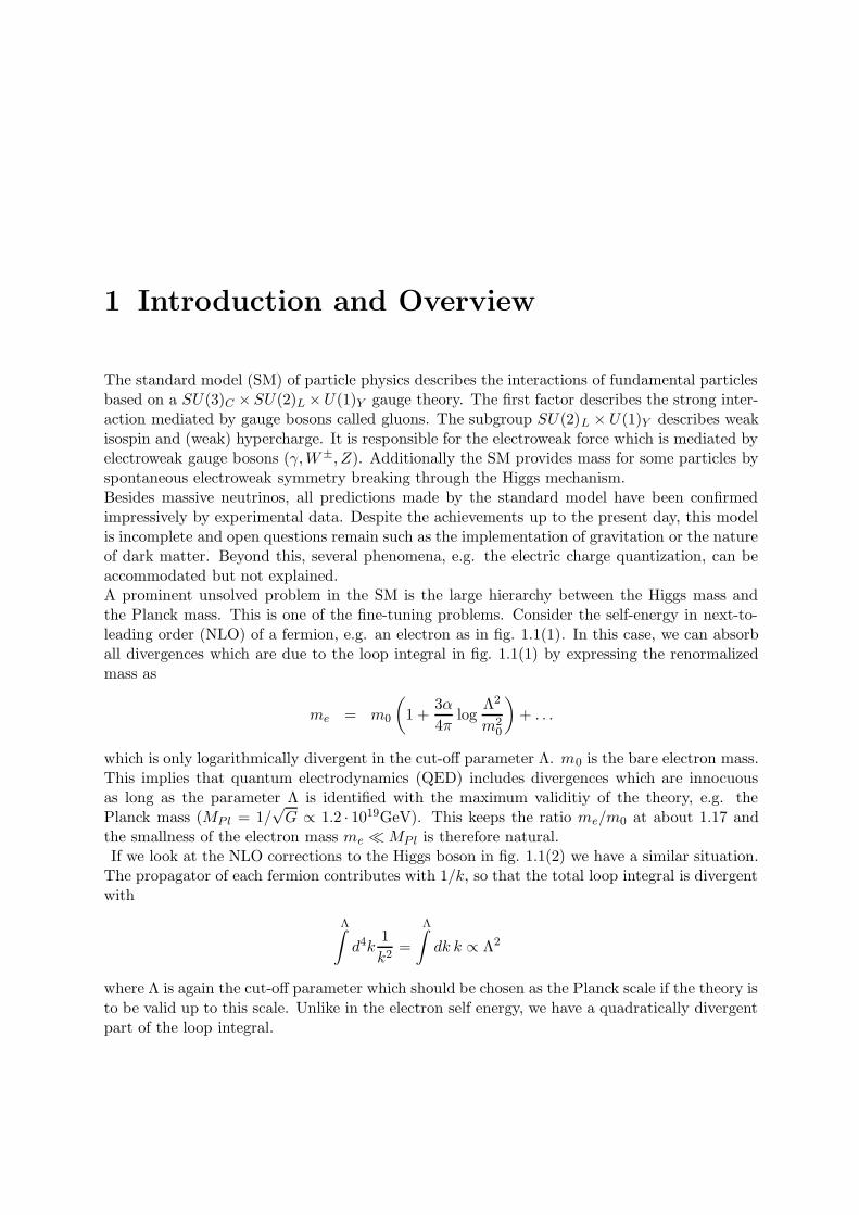
1 Introduction and Overview
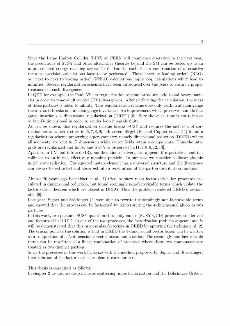
The standard model (SM) of particle physics describes the interactions of fundamental particlesbased on a SU(3)C × SU(2)L ×U(1)Y gauge theory. The first factor describes the strong inter-action mediated by gauge bosons called gluons. The subgroup SU(2)L × U(1)Y describes weakisospin and (weak) hypercharge. It is responsible for the electroweak force which is mediated byelectroweak gauge bosons (γ,W±, Z). Additionally the SM provides mass for some particles byspontaneous electroweak symmetry breaking through the Higgs mechanism.Besides massive neutrinos, all predictions made by the standard model have been confirmedimpressively by experimental data. Despite the achievements up to the present day, this modelis incomplete and open questions remain such as the implementation of gravitation or the natureof dark matter. Beyond this, several phenomena, e.g. the electric charge quantization, can beaccommodated but not explained.A prominent unsolved problem in the SM is the large hierarchy between the Higgs mass andthe Planck mass. This is one of the fine-tuning problems. Consider the self-energy in next-to-leading order (NLO) of a fermion, e.g. an electron as in fig. 1.1(1). In this case, we can absorball divergences which are due to the loop integral in fig. 1.1(1) by expressing the renormalizedmass as
me = m0
(1 +
3α
4πlog
Λ2
m20
)+ . . .
which is only logarithmically divergent in the cut-off parameter Λ. m0 is the bare electron mass.This implies that quantum electrodynamics (QED) includes divergences which are innocuousas long as the parameter Λ is identified with the maximum validitiy of the theory, e.g. thePlanck mass (MP l = 1/
√G ∝ 1.2 · 1019GeV). This keeps the ratio me/m0 at about 1.17 and
the smallness of the electron mass me �MP l is therefore natural.If we look at the NLO corrections to the Higgs boson in fig. 1.1(2) we have a similar situation.
The propagator of each fermion contributes with 1/k, so that the total loop integral is divergentwith
Λ∫d4k
1
k2=
Λ∫dk k ∝ Λ2
where Λ is again the cut-off parameter which should be chosen as the Planck scale if the theory isto be valid up to this scale. Unlike in the electron self energy, we have a quadratically divergentpart of the loop integral.

2 1 Introduction and Overview
f
γ
(1)
H0
f
(2)
H0
S
(3)
Figure 1.1: Self energy of a fermion (1) and the Higgs boson in the SM (2) and in SUSY (3).
If we consider only a fermion in the loop, the Higgs mass evaluates to
m2H = m2
H,0 −|λf |28π2
Λ2 + O(
logΛ2
m2f
)+ . . . (1.1)
where λf denotes the dominant fermion-Higgs boson coupling. Thus the contributions of thecorrection terms to the Higgs mass increase quadratically with the cut-off parameter Λ.The crucial point is that, if we choose the Planck scale as the cut-off parameter, Λ2 is of theorder of 1038 GeV2. Since the physical Higgs mass is expected to be of the order of 100GeV,the bare squared Higgs mass must be precisely set close to the Planck scale to an accuracy ofabout 32 digits since small variations of the bare Higgs mass would change the physical Higgsmass drastically.This discussion demonstrates that the SM without extension can only be valid up to energiesfar below the Planck scale without fine-tuning. An elegant solution to avoid these problems usesthe fact that boson loops and fermion loops have a relative sign.Consider a scalar coupling with a Higgs boson as in fig. 1.1(3). The contribution of this graphto the Higgs mass is divergent with λs ·Λ2 where λs is the 4-scalar coupling. Such a couplingwith λs = |λf |2 would compensate the entire Λ2 divergence in eq. 1.1. This can also be appliedto higher order processes which are beyond the scope of this discussion.The supersymmetric version of the SM extends the particle spectrum in exactly this way. SMfermions and their corresponding spin-0 partners (sfermions) form a chiral supermultiplet andthe couplings of sfermions and fermions to the Higgs boson are such that λs = |λf |2, thus provid-ing a solution to the hierarchy problem. The corresponding fermionic supersymmetric partnersof the SM gauge bosons are called gauginos and both together form the gauge supermultiplet.For further reading we refer to [3].Since no superpartners of the SM particles have been observed so far, SUSY must be softlybroken in such a way that the masses of the SM particles and their SUSY partners differ. Softbreaking means that masses and couplings may be modified only in ways that do not reintro-duce the quadratic divergences in eq. 1.1. For example, the selectron, the superpartner to theelectron, is required to be heavier than 73GeV at a confidence level of 95% [4] and therefore hasto receive a SUSY breaking mass.
3
Since the Large Hadron Collider (LHC) at CERN will commence operation in the next year,the predictions of SUSY and other alternative theories beyond the SM can be tested up to anunprecedented energy reaching several TeV. For the exclusion or confirmation of alternativetheories, precision calculations have to be performed. These “next to leading order” (NLO)or “next to next to leading order” (NNLO) calculations imply loop calculations which lead toinfinities. Several regularization schemes have been introduced over the years to ensure a propertreatment of such divergences.In QED for example, the Pauli Villars regularization scheme introduces additional heavy parti-cles in order to remove ultraviolet (UV) divergences. After performing the calculation, the massof these particles is taken to infinity. This regularization scheme does only work in abelian gaugetheories as it breaks non-abelian gauge invariance. An improvement which preserves non-abeliangauge invariance is dimensional regularization (DREG) [5]. Here the space time is not taken as4- but D-dimensional in order to render loop integrals finite.As can be shown, this regularization scheme breaks SUSY and requires the inclusion of cor-rection terms which restore it [6, 7, 8, 9]. However, Siegel [10] and Capper et al. [11] found aregularization scheme preserving supersymmetry, namely dimensional reduction (DRED) whereall momenta are kept in D dimensions while vector fields retain 4 components. Thus the inte-grals are regularized and finite, and SUSY is preserved [6, 11, 7, 8, 9, 12, 13].Apart from UV and infrared (IR), another kind of divergence appears if a particle is emittedcollinear to an initial, effectively massless particle. In our case we consider collinear gluonicinitial state radiation. The squared matrix element has a universal structure and the divergencecan always be extracted and absorbed into a redefinition of the parton distribution function.
Almost 20 years ago Beenakker et al. [1] tried to show mass factorization for processes cal-culated in dimensional reduction, but found seemingly non-factorizable terms which violate thefactorization theorem which are absent in DREG. Thus the problem rendered DRED question-able [6].Last year, Signer and Stockinger [2] were able to rewrite the seemingly non-factorizable termsand showed that the process can be factorized by reinterpreting the 4-dimensional gluon as twoparticles.In this work, two partonic SUSY quantum chromodynamics (SUSY QCD) processes are derivedand factorized in DRED. In one of the two processes, the factorization problem appears, and itwill be demonstrated that this process also factorizes in DRED by applying the technique of [2].The crucial point of the solution is that in DRED the 4-dimensional vector boson can be writtenas a composition of a D-dimensional vector boson and a scalar. The seemingly non-factorizableterms can be rewritten as a linear combination of processes where these two components aretreated as two distinct partons.Since the processes in this work factorize with the method proposed by Signer and Stoeckinger,their solution of the factorization problem is corroborated.
This thesis is organized as follows:In chapter 2 we discuss deep inelastic scattering, mass factorization and the Dokshitzer-Gribov-
4 1 Introduction and Overview
Lipatov-Altarelli-Parisi (DGLAP) equations. In addition, collinear factorization for a particularexample is introduced and calculated. In chapter 3 we give an overview and introduction toSUSY and discuss the need of dimensional reduction in MSSM processes.The result for the mass factorization in DRED of the most important processes for stop pro-duction at LHC
qq → g t t (1.2a)
gg → g t t (1.2b)
is given and discussed in chapter 4. Though the process in eq. 1.2a factorizes in DRED asexpected, the process in eq. 1.2b seems to violate the factorization theorem. From this wemotivate the separation of the 4-dimensional gluon into two partons and calculate the Feynmanrules and splitting functions for this new scalar.In chapter 5 we calculate both processes in eq. 1.2 in LO in dimensional reduction followedby the NLO calculation of the processes and the factorization in 4 dimensions and dimensionalreduction in chapter 6. We demonstrate that they factorize as desired when the method proposedin [2] is applied.After the detailed demonstration of the calculation we discuss the result in chapter 7, givecriteria for the appearance of the factorization problem and argue its absence in the masslesslimit.In chapter 8 the calculations and results are summarized.
2 QCD, DIS and the Factorization Theorem
Due to confinement no free quarks exist in nature but only color neutral bound states calledhadrons which include baryons (quark triplets) and mesons (quark pairs). This makes directquark collision experiments impossible and therefore hadron collisions have to be used to inves-tigate quark scattering.In this work we present the mass factorization of two SUSY QCD processes. For the deriva-tion of these we treat the initial partons as free particles with well defined momenta. Sincewe investigate processes which are probed at the LHC, the scattering particles are protons. Inthis chapter we will give an overview of the calculation with partons, its connection with thehadronic cross section, and we discuss mass factorization.
2.1 Deep Inelastic Scattering
At low energies a proton can be described as a spin 1/2 particle with electric charge +1 and massof about one GeV. High energy interactions (≥ 10 GeV) unveil a substructure of the proton asa bound state of quarks and gluons. When a proton is probed at these high energies, it seems tobe constituted by gluons and one down and two up quarks which define the quantum numbersof the proton and are called valence quarks.For even higher energies, the gluons split into quark antiquark pairs, and quarks radiate gluonsso that new particles are present in the parton. However, the net quark content defined as∑
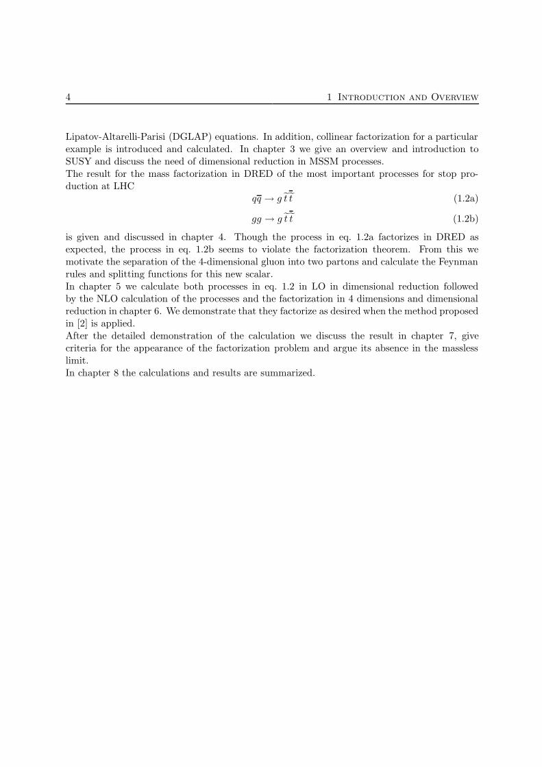
i qi − qi (i runs over the quark flavors) stays the same and still corresponds to the valencequarks. These particles, which do not alter the quantum number of the hadron, are calledsea-quarks. Scattering processes at energies which probe this partonic structure of hadrons arereferred to as deep inelastic scattering processes (DIS).Due to asymptotic freedom, short distance cross sections can be calculated perturbatively [14][15]. In the following we demonstrate how a hadronic cross section is constituted by a partoniccross section and the corresponding parton distribution functions (PDFs), which give the prob-ability to find a parton with a certain fraction of the total momentum inside the hadron. Weconsider an experiment in which two protons with momenta P1 and P2 are collided as in fig. 2.1.All constituents carry a fraction of the total hadron momentum
p1 = x1P1
p2 = x2P2

6 2 QCD, DIS and the Factorization Theorem
x2P2
x1P1
P2
P1
Figure 2.1: Deep inelastic scattering of protons. At energies above 10GeV the substructure canbe tested and the proton collision can be described by a collision of two quarks orgluons, each carrying a fraction xi Pi of the proton momentum Pi. The arrows standfor the flow of momenta.
where xi is between 0 and 1. The cross section for hard scattering processes with initial hadronmomenta P1 and P2 can be written as
σ (p(P1) + p(P2) → X + Y ) =
(2.1)1∫
0
dx1
1∫
0
dx2
∑
i,j
fi(x1, µ)fj(x2, µ) · σ (qi(x1P1) + qj(x2P2) → Y )
The momenta are defined as they appear in fig. 2.1. Consequently, the cross section for twohadrons is the result of the cross section between quarks or gluons as the constituents of theincoming hadrons. The functions fi(xj , µ) which give the probability of finding the constituentwith the fraction xj of the momentum, namely the quark and gluon distribution inside thehadron, are known as the parton distribution functions (PDFs). They are defined at a factor-ization scale µ, which is a parameter that separates the long (hadronic) and short (partonic)distance physics.
Equation 2.1 implies, that the long distance hadronic cross section can be expressed in terms ofthe short distance cross section by separating long distance pieces (e.g. collinear gluon radiation)by absorbing them into the PDFs. This separation into the partonic short distance cross sectionand the PDF (eq. 2.1) is referred to as the factorization theorem and was proven by Collins andSoper to all orders of perturbation theory [16].The short distance cross section is independent from the details or type of the incoming hadronand can be calculated perturbatively. This implies that we can use ordinary QCD Feynman rulesfor the short distant part of the calculation of hadron scattering. For a detailed description of
2.2 Collinear Divergences 7
DIS we refer to [17].The PDF fi(xj , µ) can not be calculated from perturbative QCD, since the strongly interactingphysics of bound hadrons enters the calculation. This is why the PDFs have to be obtained byfitting the parton model predictions to experimental data. In the next sections, we will discussthat the PDFs depend on the factorization scale µ and sketch the derivation of the DGLAPequations which give the evolution of the PDFs with this energy scale µ2.
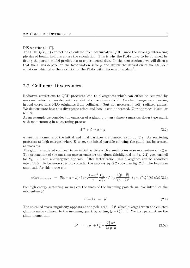
2.2 Collinear Divergences
Radiative corrections to QCD processes lead to divergences which can either be removed byrenormalization or canceled with soft virtual corrections at NLO. Another divergence appearingin real corrections NLO originates from collinearly (but not necessarily soft) radiated gluons.We demonstrate how this divergence arises and how it can be treated. Our approach is similarto [18].As an example we consider the emission of a gluon g by an (almost) massless down type quarkwith momentum q in a scattering process
W+ + d→ u+ g (2.2)
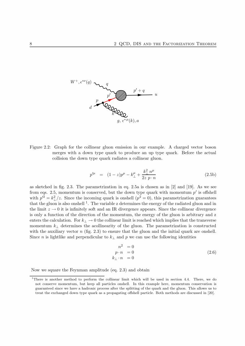
where the momenta of the initial and final particles are denoted as in fig. 2.2. For scatteringprocesses at high energies where E � m, the initial particle emitting the gluon can be treatedas massless.The gluon is radiated collinear to an initial particle with a small transverse momentum k⊥ � µ.The propagator of the massless parton emitting the gluon (highlighted in fig. 2.2) goes onshellfor k⊥ → 0 and a divergence appears. After factorization, this divergence can be absorbedinto PDFs. To be more specific, consider the process eq. 2.2 shown in fig. 2.2. The Feynmanamplitude for this process is
MW++d→g+u = v(p+ q − k) · i e γν1 − γ5
2
Vij√2s
· ε∗ ν(q)i(/p− /k)
(p− k)2· i g γµ t
a ε∗µa (k)u(p) (2.3)
For high energy scattering we neglect the mass of the incoming particle m. We introduce themomentum p′
(p− k) = p′ (2.4)
The so-called mass singularity appears as the pole 1/(p − k)2 which diverges when the emittedgluon is made collinear to the incoming quark by setting (p− k)2 = 0. We first parametrize thegluon momentum
kµ = zpµ + kµ⊥ − k2
⊥ nµ
2z p ·n (2.5a)
8 2 QCD, DIS and the Factorization Theorem
p
q
p′ + qp′
k
d
W+, ε∗ν(q)
u
g, ε∗µ(k), a
Figure 2.2: Graph for the collinear gluon emission in our example. A charged vector bosonmerges with a down type quark to produce an up type quark. Before the actualcollision the down type quark radiates a collinear gluon.
p′µ = (1 − z)pµ − kµ⊥ +
k2⊥ n
µ
2z p ·n (2.5b)
as sketched in fig. 2.3. The parametrization in eq. 2.5a is chosen as in [2] and [19]. As we seefrom eqs. 2.5, momentum is conserved, but the down type quark with momentum p′ is offshellwith p′2 = k2
⊥/z. Since the incoming quark is onshell (p2 = 0), this parametrization guaranteesthat the gluon is also onshell 1. The variable z determines the energy of the radiated gluon and inthe limit z → 0 it is infinitely soft and an IR divergence appears. Since the collinear divergenceis only a function of the direction of the momentum, the energy of the gluon is arbitrary and zenters the calculation. For k⊥ → 0 the collinear limit is reached which implies that the transversemomentum k⊥ determines the acollinearity of the gluon. The parametrization is constructedwith the auxiliary vector n (fig. 2.3) to ensure that the gluon and the initial quark are onshell.Since n is lightlike and perpendicular to k⊥ and p we can use the following identities
n2 = 0p ·n = 0
k⊥ ·n = 0(2.6)
Now we square the Feynman amplitude (eq. 2.3) and obtain
1There is another method to perform the collinear limit which will be used in section 4.4. There, we donot conserve momentum, but keep all particles onshell. In this example here, momentum conservation isguaranteed since we have a hadronic process after the splitting of the quark and the gluon. This allows us totreat the exchanged down type quark as a propagating offshell particle. Both methods are discussed in [20].
2.2 Collinear Divergences 9
n
k
p−k
k
p
Figure 2.3: Illustration of the vectors n and k⊥ parametrizing the collinear limit of the particleswith the momenta p and k. n is an auxiliary lightlike vector which is perpendicularto k⊥.
|M|2W++d→g+u = M†(/p− /k)γµu(p)u(p)γµ′(/p− /k)M ε∗µa (k)εµ
′
a′ (k)
(p− k)4Cs(r)δ
aa′
Here M† stands for the expression
M† = u(p′ + q) · e γν1 − γ5
2
Vij√2s
· ε∗ ν(q)
and will later give the amplitude in eq. 2.10. Since the incoming down type quark is onshellwith p2 = 0 we can use eq. A.13 for massless quarks
|M|2W++d→g+u = M†(/p− /k)γµ /p γµ′(/p− /k)M ε∗µa (k)εµ
′
a′ (k)
(p− k)4C2(r)δ
aa′
(2.7)
We use the polarization sum for massless gauge bosons
∑
s=1,2
ε∗µs (k)εµ
′
s (k) = −gµµ′
+kµnµ′
+ kµ′nµ
k ·n (2.8)
First, we insert the metric tensor from eq. 2.8 into eq. 2.7, denoting this part with A:
A = M†(/p− /k)γµ/p γ
µ′
(/p− /k)M(−gµµ′)
= −M†(/p− /k)γµ/p γµ(/p− /k)M
10 2 QCD, DIS and the Factorization Theorem
A1
= 2M†(/p− /k) /p (/p− /k)M2
= 2M† /k /p /k M1
= 4M†/kM p · k
Now we can express the momentum k as
k =z
1 − zp′
which follows from the parametrization of the momenta in eq. 2.5. Obviously, M containsno poles of the form 1/(p − k) and therefore we can neglect all terms containing k⊥ in thissubstitution. Now we substitute p′ and k using eq. 2.5 and obtain
A = 4M† /p′M z
1 − z· −k
2⊥
2z
= −2|M|2W++d→u
k2⊥
(1 − z)(2.9)
where |M|2W++d→u
is defined with
MW++d→u = M† /p′M (2.10)
and represents the scattering process W+ + d→ u.
Now we insertkµnµ′
k ·n from eq. 2.8 into eq. 2.7
B = M†(/p− /k)γµ/pγ
µ′
(/p− /k)M(kµnµ′
k ·n )
= M†(/p− /k) /k /p /n(/p− /k)M 1
k ·n3
,4
= M†/p /k /p /n /pM
1 − z
k ·n5
= 4M†/pM n · p k · p1 − z
k ·n6
= 2|M|2W+d→u ·−k2
⊥z2
(2.11)
1with /p /k /p = pµ kν pρ (γµγνγρ) = pµ kν pρ (γµ(γνγρ + γργν) − γµγργν) = pµ kν pρ (γµ2gνρ − γµγργν) =
/p 2k · p − /p/p/k.2with /p/p = 0 since p2 = 0
2.2 Collinear Divergences 11
The third part of eq. 2.8 gives the same result as eq. 2.11. Now we add both squared amplitudesgiven in eq. 2.9 and eq. 2.11
|M|2W++d→g+u =1
(p− k)4(A+ 2B) ·C2(r)
〈k||p〉7=
=−2 z2
k4⊥
|M|2W+d→u · k2⊥ ·(
2
z2+
1
(1 − z)
)·C2(r)
= −2|M|2W+d→u ·z2
(1 − z)k2⊥· z
2 − 2z + 2
z·C2(r) (2.12)
The last factor C2(r) · (z2−2z+2)/z of eq. 2.12 can be identified with the gluon-quark splittingfunction. We notice that the squared amplitude |MW++d→u+g|2 is proportional to the matrixelement |MW++d→u|2 in the collinear limit. The factorization of this process into the divergence,the splitting function and the LO cross section is called mass factorization.The cross section from the process in fig. 2.2 is then
dσW++d→u+g ∝∫
d3k
(2π)32Ek· z2
(1 − z)k2⊥· z
2 − 2z + 2
z(1 − z) dσW++d→u
where the phase space integral of the other three particles is contained in dσW++d→u. The factor(1 − z) corrects the flux factor for the cross section dσW++d→u, since the incoming momentumfor this cross section is (1 − z)p rather than p.The integration of the gluon phase space can be decomposed into
d3k
(2π)32Ek=
dz dφ dk2⊥
4(2π)3z+ O(k2
⊥)
Since the cross section is independent of the angle φ, the integration over dφ yields a factor 2πand we find
dσW++d→u+g ∝∫dk2
⊥k2⊥
∫ 1
0dzz2 − 2z + 2
zdσW++d→u
∝ log(k2⊥)∣∣∣∣
k2⊥,max
k2⊥,min
1∫
0
dz
(z2 − 2z + 2
zdσW++d→u
)(2.13)
3the first p − k is set to p since /k/k = 0 as k2 = 04the second p − k is rewritten using eq. 2.5 and substituted with p − k = (1 − z)p, since n · k⊥ = 0 and n2 = 0.5we use /p /k /p /n /p = pµ kν pρ nσ pτ (γµγνγργσγτ ) = pµ kν pρ nσ pτ (γµγνγρ(γσγτ + γτγσ) − γµγνγργτγσ) =
pµ kν pρ nσ pτ (γµγνγρ2gστ − γµγνγργτγσ) = pµ kν pρ nσ pτ (2gστ (γµ(γνγρ + γργν) − γµγργν)) =pµ kν pρ nσ pτ (2gστ (γµ2gνρ − γµγργν)) = 4/p n · p k · p
6k · p = −k2⊥/2/z, k ·n = z n · p and fM†
/p fM = fM† /p′ fM/(1 − z) = | fM|2W+d→u
/(1 − z)7Denoting that the particle with momentum k is collinear to the particle with momentum p.

12 2 QCD, DIS and the Factorization Theorem
The upper limit of the transverse phase space integration is determined by Q, the energy scaleof the process. Since we set all particle masses to zero, the lower limit is zero and representsthe collinear singularity. If the particle mass is finite, the lower limit is of the order of this massand the singularity is regularized. The collinear singularity is then parametrized with the massof the emitting particle.We finally find for the cross section
dσq+qi→qj+qf∝ log
(Q2
m2
)∫ 1
0dz Pji(z) dσq+qi→qf
(2.14)
The factor Pji(z) is called splitting function and depends on the vertex structure of the radiatedand emitting particles. For different particles, e.g. quarks, gluons, or electrons radiating gluonsor photons we need different splitting functions which depend on the particular vertex structure.We will calculate the splitting functions needed for this work in chapter 4.4.
These results for the cross section given in eq. 2.14 have a physical interpretation which isrelated to the hadron picture described in section 2.1. The cross section with a collinear particle(e.g. gluon or photon) in the final state factorizes into the splitting function Pji(z), the pole andthe LO cross section. After having radiated collinearly, the particle enters the short distancecross section with momentum fraction (1 − z), while the collinear divergence is absorbed intothe PDFs.
Summarizing these results, mass factorization predicts that a NLO cross section factorizes intoa collinear pole, the corresponding LO process and a splitting function. In terms of the squaredamplitude |M|2 this can be expressed as
|M|2pa+pb→g+pc+pd
〈k2||k3〉= |M|2pa+pb→pc+pd
· 1t1(1−z) ·Pji(z) (2.15)
where 1/t1(1− z) is the mass singularity2 arising from the propagator and Pji(z) is the splittingfunction. The Mandelstam variable t1 is defined in eq. A.4. The pole enters the parton distri-bution functions and changes the probability of finding a parton inside another parton. Eachparton can therefore absorb or emit any amount of other collinear partons. These effects leadto a dependence of the PDFs on the energy scale Q2 in shape and magnitude.
Heuristically, mass factorization can be explained by the fact that collinearly emitted particlescan not be detected in a measurement since they are in the direction of the beam line. Thisimplies that the real NLO 2 → 3 process with a collinear final particle can not be distinguishedexperimentally from the LO 2 → 2 process.
2The factor 1/(1-z) is always factored out in the following calculations. This factor corrects the flux for thedifferential cross section.
2.3 Multiple Splitting and Evolution Equations 13
2.3 Multiple Splitting and Evolution Equations
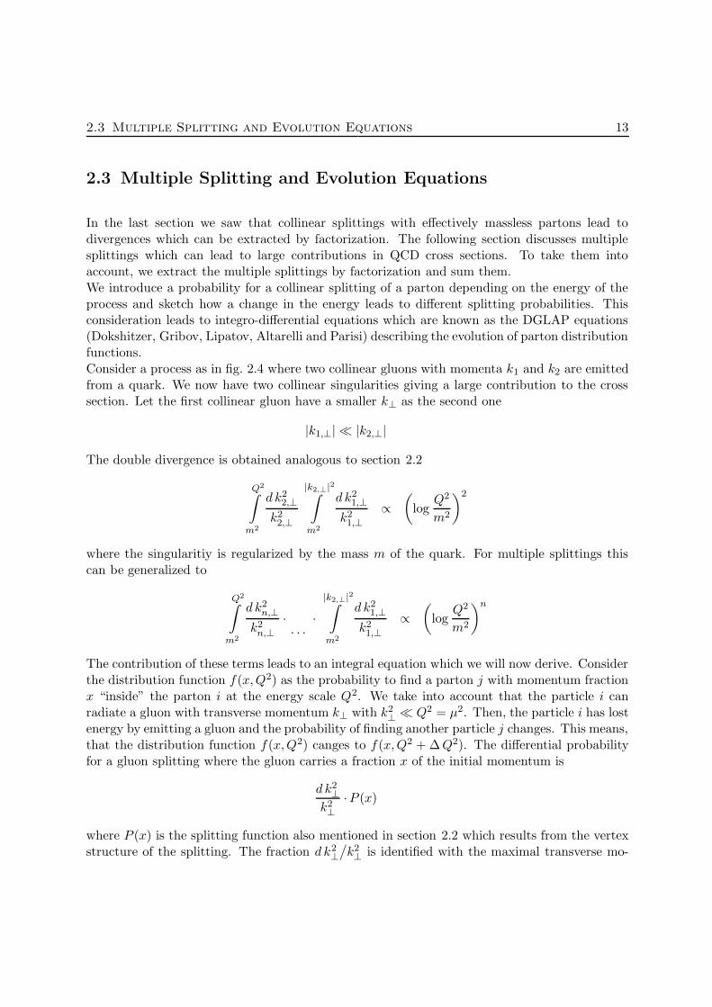
In the last section we saw that collinear splittings with effectively massless partons lead todivergences which can be extracted by factorization. The following section discusses multiplesplittings which can lead to large contributions in QCD cross sections. To take them intoaccount, we extract the multiple splittings by factorization and sum them.We introduce a probability for a collinear splitting of a parton depending on the energy of theprocess and sketch how a change in the energy leads to different splitting probabilities. Thisconsideration leads to integro-differential equations which are known as the DGLAP equations(Dokshitzer, Gribov, Lipatov, Altarelli and Parisi) describing the evolution of parton distributionfunctions.Consider a process as in fig. 2.4 where two collinear gluons with momenta k1 and k2 are emittedfrom a quark. We now have two collinear singularities giving a large contribution to the crosssection. Let the first collinear gluon have a smaller k⊥ as the second one
|k1,⊥| � |k2,⊥|
The double divergence is obtained analogous to section 2.2
Q2∫
m2
d k22,⊥
k22,⊥
|k2,⊥|2∫
m2
d k21,⊥
k21,⊥
∝(
logQ2
m2
)2
where the singularitiy is regularized by the mass m of the quark. For multiple splittings thiscan be generalized to
Q2∫
m2
d k2n,⊥
k2n,⊥
·. . .
·|k2,⊥|2∫
m2
d k21,⊥
k21,⊥
∝(
logQ2
m2
)n
The contribution of these terms leads to an integral equation which we will now derive. Considerthe distribution function f(x,Q2) as the probability to find a parton j with momentum fractionx “inside” the parton i at the energy scale Q2. We take into account that the particle i canradiate a gluon with transverse momentum k⊥ with k2
⊥ � Q2 = µ2. Then, the particle i has lostenergy by emitting a gluon and the probability of finding another particle j changes. This means,that the distribution function f(x,Q2) canges to f(x,Q2 + ∆Q2). The differential probabilityfor a gluon splitting where the gluon carries a fraction x of the initial momentum is
d k2⊥
k2⊥
·P (x)
where P (x) is the splitting function also mentioned in section 2.2 which results from the vertexstructure of the splitting. The fraction d k2
⊥/k2⊥ is identified with the maximal transverse mo-
14 2 QCD, DIS and the Factorization Theorem
qj qk
p · z, f(z,Q2)
p · yz = p ·x, f(x,Q2)
p(1 − z) · p
(1 − y)z · p
Figure 2.4: Graph for the double collinear gluon emission.
mentum dQ2/Q2.
For the distribution function at the energy Q2 + dQ2 we find with fig. 2.4
f(x,Q2 + ∆Q2) = f(x,Q2) +
1∫
0
dy
1∫
0
dz δ(x− yz)α
2π
dQ2
Q2·P (y)f(z,Q2)
This term is a compound of the parton distribution for the parton with momentum fractionz at energy Q2 and the probability for splitting off a particle with momentum fraction y. Weintegrate this over all possible momenta z and y. The δ-function enters the term to guaranteemomentum conservation. After evaluating the integral over y we obtain
f(x,Q2 + ∆Q2) = f(x,Q2) +dQ2
Q2
α
2π
∫ 1
x
dz
zP(xz
)f(z,Q2) (2.16)
This leads to the integro-differential equation
d
d(logQ2)f(x,Q2) =
α
2π
∫ 1
x
dz
zP(xz
)f(z,Q2) (2.17)
which describes the Q2 dependence of the parton distribution function for an initial distributionf(x,m2).
Thus the parton distribution functions in eq. 2.1 do not only have an x dependence but also aµ2 = Q2 dependence. In early experiments (fig. 2.6) no Q2 dependence was observed due to thelimited energy range. This phenomenon which was a supporting evidence for the naive partonmodel is referred to as Bjorken scaling. It was only in more recent experiments that the Q2
dependence derived above (Bjorken scaling violation) was observed (fig. 2.5). For the large

2.3 Multiple Splitting and Evolution Equations 15
HERA F2
0
1
2
3
4
5
1 10 102
103
104
105
F 2 em-lo
g 10(x
)
Q2(GeV2)
ZEUS NLO QCD fit
H1 PDF 2000 fit
H1 94-00
H1 (prel.) 99/00
ZEUS 96/97
BCDMS
E665
NMC
x=6.32E-5 x=0.000102x=0.000161
x=0.000253x=0.0004
x=0.0005x=0.000632
x=0.0008
x=0.0013
x=0.0021
x=0.0032
x=0.005
x=0.008
x=0.013
x=0.021
x=0.032
x=0.05
x=0.08
x=0.13
x=0.18
x=0.25
x=0.4
x=0.65
Figure 2.5: The results for the structure function F em2 versus Q2 are shown for fixed x [21].
16 2 QCD, DIS and the Factorization Theorem
Figure 2.6: Scaling behaviour of the structure function F2 as found in experiments at SLAC inthe early 1970s (according to [22])
energy limit of the PDF one found
f(x,Q2)|Q2→∞,x→0 = ∞f(x,Q2)|Q2→∞,x→1 = 0
This means, that with increasing energy Q2 we find less quarks with high momentum fractionin the hadron, but we have a large number of partons each carrying a smaller fraction of thetotal momentum. This is due to the fact that at higher energies the probability for emission orabsorption of gluons by partons and the creation of new quark pairs increases.The equations describing the full Q2 dependence of the hadron PDFs were derived by Dokshitzer,Gribov, Lipatov, Altarelli and Parisi [23] [24] [25] and are referred to as DGLAP or Altarelli-Parisi equations. They are an extension of eq. 2.17 for quarks and gluons in the context ofhadron scattering taking into account gluon-gluon, gluon-quark and quark-gluon splitting.
2.3 Multiple Splitting and Evolution Equations 17
0.2 0.4 0.6 0.8 1x
0.2
0.4
0.6
0.8xf
@xD
400 GeV2
40 GeV2
4 GeV2
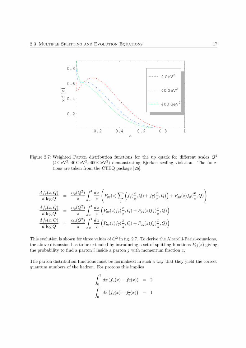
Figure 2.7: Weighted Parton distribution functions for the up quark for different scales Q2
(4GeV2, 40GeV2, 400GeV2) demonstrating Bjorken scaling violation. The func-tions are taken from the CTEQ package [26].
d fg(x,Q)
d logQ=
αs(Q2)
π
∫ 1
x
d z
z
(Pgq(z)
∑
q
(fq(
x
z,Q) + fq(
x
z,Q)
)+ Pgg(z)fg(
x
z,Q)
)
d fq(x,Q)
d logQ=
αs(Q2)
π
∫ 1
x
d z
z
(Pqq(z)fq(
x
z,Q) + Pqg(z)fg(
x
z,Q)
)
d fq(x,Q)
d logQ=
αs(Q2)
π
∫ 1
x
d z
z
(Pqq(z)fq(
x
z,Q) + Pqg(z)fg(
x
z,Q)
)
This evolution is shown for three values of Q2 in fig. 2.7. To derive the Altarelli-Parisi-equations,the above discussion has to be extended by introducing a set of splitting functions Pij(z) givingthe probability to find a parton i inside a parton j with momentum fraction z.
The parton distribution functions must be normalized in such a way that they yield the correctquantum numbers of the hadron. For protons this implies
∫ 1
0dx (fu(x) − fu(x)) = 2
∫ 1
0dx(fd(x) − fd(x)
)= 1
18 2 QCD, DIS and the Factorization Theorem
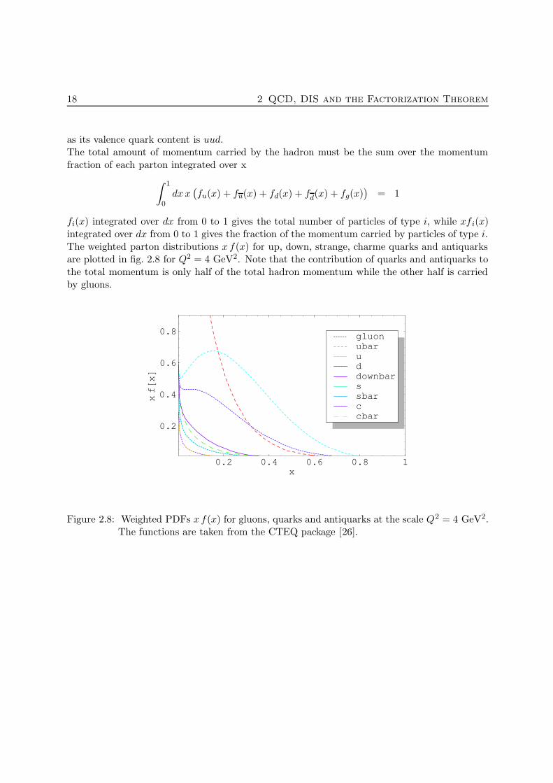
as its valence quark content is uud.The total amount of momentum carried by the hadron must be the sum over the momentumfraction of each parton integrated over x
∫ 1
0dxx
(fu(x) + fu(x) + fd(x) + fd(x) + fg(x)
)= 1
fi(x) integrated over dx from 0 to 1 gives the total number of particles of type i, while xfi(x)integrated over dx from 0 to 1 gives the fraction of the momentum carried by particles of type i.The weighted parton distributions x f(x) for up, down, strange, charme quarks and antiquarksare plotted in fig. 2.8 for Q2 = 4 GeV2. Note that the contribution of quarks and antiquarks tothe total momentum is only half of the total hadron momentum while the other half is carriedby gluons.
0.2 0.4 0.6 0.8 1x
0.2
0.4
0.6
0.8
xf
@xD
cbarcsbarsdownbarduubargluon
Figure 2.8: Weighted PDFs x f(x) for gluons, quarks and antiquarks at the scale Q2 = 4 GeV2.The functions are taken from the CTEQ package [26].
3 Supersymmetry and Regularization
Schemes
The simplest and most popular realistic supersymmetric model is the straightforward introduc-tion of supersymmetric particles to the SM. Only those couplings and fields that are necessaryand sufficient for the consistency of the theory are included. This model is called minimal su-persymmetric standard model (MSSM). Before we introduce the MSSM we will discuss a toymodel to illustrate how field theories are made supersymmetric.
3.1 A Supersymmetric Toy Model
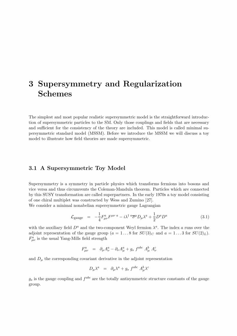
Supersymmetry is a symmetry in particle physics which transforms fermions into bosons andvice versa and thus circumvents the Coleman-Mandula theorem. Particles which are connectedby this SUSY transformation are called superpartners. In the early 1970s a toy model consistingof one chiral multiplet was constructed by Wess and Zumino [27].We consider a minimal nonabelian supersymmetric gauge Lagrangian
Lgauge = −1
4F a
µνFµν a − iλ† aσµDµλ
a +1
2DaDa (3.1)
with the auxiliary field Da and the two-component Weyl fermion λa. The index a runs over theadjoint representation of the gauge group (a = 1 . . . 8 for SU(3)C and a = 1 . . . 3 for SU(2)L).F a
µν is the usual Yang-Mills field strength
F aµν = ∂µA
aν − ∂νA
aµ + gs f
abc Abµ A
cν
and Dµ the corresponding covariant derivative in the adjoint representation
Dµλa = ∂µλ
a + gs fabc Ab
µλc
gs is the gauge coupling and f abc are the totally antisymmetric structure constants of the gaugegroup.

20 3 Supersymmetry and Regularization Schemes
The action∫d4xLgauge is invariant under the following SUSY transformations
δAaµ = 1√
2
(ε†σµλ
a + λ† aσµε)
δλaα = i
2√
2(σµσνε)α F
aµν + 1√
2εαD
a
δDa = i√2
(ε†σµDµλ
a −Dµλ† aσµε
)(3.2)
So far, all particles in a multiplet have the same mass. Since to date no superpartners ofSM particles have been found which would be inevitable if they had the same mass, a SUSYbreaking mechanism must be part of any realistic model. One can for example construct theminimal supersymmetric standard model (MSSM) based on the SM in which the masses ofall supersymmetric partners can be increased by SUSY breaking terms to satisfy experimentalconstraints.
3.2 Description of the MSSM
In the following we give a brief description of the MSSM particle content which represents theminimal number of fields necessary to formulate a supersymmetric extension of the SM.The mechanism that gives mass to the up type fermions in the SM can not be used in theMSSM as it would be incompatible with SUSY. Therefore we need two Higgs doublets with 8real degrees of freedom. Three of them are eaten by the massive gauge bosons and 5 remain asphysical Higgs bosons. The two doublets come with 4 spin-1/2 partners called higgsinos.
The superpartners of the electroweak gauge bosons are the spin-1/2 Bino (B) and Wino (W 1,2,3).The gauginos, like the higgsinos, are not mass eigenstates and together they form 4 Majorananeutralinos and two Dirac charginos.The SUSY partners of the left- and righthanded Quarks (qL and qR) are the left- and righthandedsquarks (qL and qR). They transform under SU(2)L × U(1)Y and also under the fundamentalrepresentation of the QCD gauge group SU(3)C like the quarks.The SUSY partners of the leptons are the sleptons. They both transform under the fundamentalrepresentation of the SU(2)L × U(1)Y .The group representations of all particles are summarized in tab. 3.1. The fact that none of thesesupersymmetric particles have been found so far leads to the conclusion that supersymmetrymust be broken and superpartners differ in mass from their SM particles. The mechanism forSUSY breaking is not yet known but we can parametrize it by introducing the most generalbreaking terms which nevertheless preserve the solution for the hierarchy problem as discussedin chapter 1.The effective Lagrangian for softly broken SUSY can be written as
L = LSUSY + Lsoft

3.2 Description of the MSSM 21
Gauge Group SM Field s Super- s Super-partner field
U(1)Y , adj. repr. B 1 B 1/2 V1
SU(2)L, adj. repr. W 1,2,3 1 W 1,2,3 1/2 V2
SU(2)L × U(1)Y , fund. repr. (ν, e)L 1/2 (ν, e)L 0 L
SU(3)C × SU(2)L × U(1)Y , fund. repr. (u, d)L 1/2 (u, d)L 0 Q
U(1)Y , fund. repr. eR 1/2 eR 0 Ec,
SU(3)C × U(1)Y , fund. repr. uR, dR 1/2 uR, dR 0 U c, Dc
SU(3)C , adj. repr. g 1 g 1/2 V3
SU(2)L × U(1), fund. repr. (φ+, hd + iφ3) 0 (φ+, hd) 1/2 H1
Extended Higgs sector in MSSMSU(2)L × U(1), fund. repr. (hu + iA,H−) 0 (hu, H−) 1/2 H2
Table 3.1: Standard model particles and their corresponding superpartners with spin, superfieldand gauge group.
The explicit form of the most general soft SUSY breaking terms is
Lsoft = −(
1
2Maλ
aλa +1
6aijkφiφjφk +
1
2bijφiφj + tiφi
)
+c.c.− (m2)ijφj∗φi (3.3)
All other possible mass terms are redundant and can be absorbed into a redefinition of thesuperpotential and the coefficients in eq. 3.3. Ma stands for the different gaugino masses, aijk
are the three scalar and bij the two scalar couplings. The tadpole coupling is represented by ti,the scalar mass terms by m2i
j.
The SUSY Lagrangian can contain couplings between two SM and one SUSY particle. Thiscoupling leads to undesired effects like quick proton decay. However, the current bound of pro-ton decay is > 1031 to 1033 years [4]. So, in the MSSM these coupling have to be forbidden orremoved by enforcing a new discrete symmetry, which is called R parity. This number is definedfor each particle as
R = (−1)3(B−L)+2S
where B denotes the baryon number, L the lepton number and S stands for the spin of theparticle. This number gives +1 for SM particles and −1 for SUSY partners. Terms in theLagrangian are only permitted if the product of the R parities gives +1. In other words, R parityforbids couplings where an odd number of SUSY lines meet. This new parity implies that there
22 3 Supersymmetry and Regularization Schemes
is a lightest stable SUSY particle (LSP) with parity −1. It turns out that the LSP can also actas a good dark matter candidate, but for this it is required to be electrically neutral and weaklyinteracting. All other SUSY particles decay into an uneven number of LSPs. Furthermore, thisimplies that only even numbers of SUSY particles can be produced at colliders.
3.3 Regularization and SUSY
An important technical point is the choice of the renormalization and regularization method inSUSY. In this section we will discuss that the most popular regularization scheme, dimensionalregularization (DREG), breaks SUSY. Then we will review an extension of DREG that preservesit.
Higher order calculations such as real and virtual NLO calculations involve divergent termswhich need to be regularized to be manageable. After regularizing, the expressions have to berenormalized, which means consistently subtracting infinite terms according to a special renor-malization scheme. The result must be independent from the regularization scheme since it is aphysical observable. There are two different types of divergences which have to be regularized,namely UV and IR divergences.For amplitudes including one or more loops we have to integrate over the loop momenta.Schematically, a loop integral can be of the form
Λ∫d4k
1
k4
Λ∫d4k
1
k4∝
Λ∫dkk3
k4∝
Λ∫dk
1
k∝ log Λ (3.4)
For a large momentum k the integral diverges logarithmically, which is a UV divergence. Forsmall momentum k → 0 the integral diverges as well which is known as an IR divergence. Itappears if massless particles propagating in the loop become soft. This divergence cancels withanother originating from the emission of soft massless particles in the same order of perturbationtheory, called bremsstrahlung. Meanwhile, the calculation can be performed by giving a smallmass to the massless particle which is set to zero in the end.Managing UV divergences usually requires regularization and subsequent renormalization.There are different regularization schemes which are adapted to particular applications. A simplescheme is the introduction of a cut-off parameter Λ as the maximum limit in eq. 3.4, so that theresult depends on the logarithm of Λ. This method breaks Lorentz and gauge invariance.A solution that was used for early QED calculations is the Pauli Villars regularization wherefictitious heavy particles are introduced to ensure proper cancellation of divergences. Afterperforming the calculation, the mass of the fictitious particle is taken to infinity. This methodworks only in abelian gauge theories as it breaks nonabelian gauge invariance. For furtherreading we refer to [28].Another popular regularization method that manifestly preserves gauge invariance and thereforecan be used in QCD and electroweak theory has its origin in power counting. The degree ofdivergence can be estimated by counting the mass dimensions. This means that a loop integral

3.3 Regularization and SUSY 23
Dimension Vector Spinor
2 0 8 · 23 8 · 1 8 · 24 8 · 2 8 · 25 8 · 3 8 · 4
Table 3.2: Degrees of freedom in integer dimensions for the SU(3) gauge group. The degrees offreedom for vectors and spinors depend differently on the dimension of space time.
can be made finite by evaluating it in different spacetime dimensions
∫d4k
(2π)4−→
∫dDk
(2π)4
This was the idea of t’Hooft and Veltman in 1972 [5]. The approach is the following: AllFeynman diagrams are calculated as a function of the spacetime dimensionD and the amplitudesare analytically continued to non-integer values of D. For sufficiently small D, all integrals willconverge, and the final result will be well defined for D → 4.This popular method is known as dimensional regularization (DREG) and has no importantshortcomings in SM calculations. However, using this method in the MSSM leads to seriousproblems.DREG explicitly breaks SUSY since the number of degrees of freedom of gauge bosons andgauginos do not match for D 6= 4. Let’s look at the Lagrangian from eq. 3.1 to illustrate thisissue
Lgauge = −1
4F a
µνFµν a
︸ ︷︷ ︸(1)
− iλ† aσµDµλa
︸ ︷︷ ︸(2)
+1
2DaDa
︸ ︷︷ ︸(3)
The onshell degrees of freedom for the field strength (1) are 8 · (D − 2). The 8 has its originin the dimension of the gauge group SU(3) which is (N 2 − 1) = 8. Offshell there would be Ddegress of freedom, but subtracting two degrees for the momentum direction and the energy, weget (D − 2). The fermion (2) has 8 · 2 degress of freedom onshell as it is a Weyl spinor. Theauxiliary field (3) has obviously no degree of freedom onshell since it has no kinetic term. Wesee now that in 4 dimensions the number of the gauge field degress of freedom (1) is the sameas for its superpartner (2). Otherwise, the SUSY transformation eq. 3.2 would lose degrees offreedom.For D 6= 4 dimensions, the degrees of freedom are apparently not the same. In tab. 3.2 onecan see how the degrees of freedom for a vector and a spinor change with dimension. Thisviolation of SUSY can be corrected in practical calculations by adding supersymmetry restoringcounterterms, whose existence is always guaranteed by the renormalizability of supersymmetricgauge theories. Nevertheless, these counterterms pose practical complications and are difficult
24 3 Supersymmetry and Regularization Schemes
to calculate and to implement [6, 7, 8, 9].To avoid these complications, we can use another method to regularize divergences in SUSYnamely regularization by dimensional reduction (DRED) [10] [11]. This regularization schemeleaves the vector fields 4-dimensional to maintain the match with the gaugino degrees of free-dom. In contrast, the momenta are calculated in D dimensions as in DREG. This ensures thatthe loop integrals converge while presevering SUSY at the same time.
For practical reasons we can split the four dimensional vector field Aµ in DRED into a Ddimensional vector field and a field which is effectively a scalar in D dimensions.
AµAµ = AσAσ +AiAi µ ∈ 4, σ ∈ D, i ∈ 4 −D
This component Ai of the gluon behaves like a particle of its own, and is called ε scalar. As forthe other particles we can calculate Feynman rules for this scalar, which will be done in section4.3. We can therefore calculate different amplitudes, one with D-dimensional gluons and onewith the ε scalar. However, before calculating the hadronic cross section by convolution withthe PDFs, all processes corresponding to a physical one have to be summed up. This impliesthat there is no PDF for ε scalars. Keeping this in mind, we thus call the ε scalar a parton ofits own.This method (calculating the vector bosons in D dimensions and adding a new particle to coverthe remaining (4 −D) degress of freedom) is equivalent to the somewhat awkward approach ofleaving the vector boson in 4 dimensions while the momenta are calculated in D dimensions.As mentioned at the beginning, Beenakker et al. [1] found non-factorizable terms in a massiveQCD process calculated in DRED. In the next chapter we will consider non-factorizable terms
appearing in the real NLO QCD process gg → g t t which are similar to the terms found in [1].

4 The Factorization Problem in DRED and
its Remedy
Beenakker et al. found a problem concerning the factorization theorem when using DRED knownas the factorization problem [1]. The real NLO corrections for the process gg → tt were calculatedusing DRED and DREG. For the collinear limit they found non-factorizable terms which couldnot be absorbed as a constant contribution to the PDFs. In this chapter we find similar non-
factorizable terms in the real NLO corrections to gg → t t and we will demonstrate how thisproblem can be solved analogous to [2].For this purpose we now only state the results while the derivation of the NLO amplitude andthe factorization is demonstrated in detail in chapter 6.
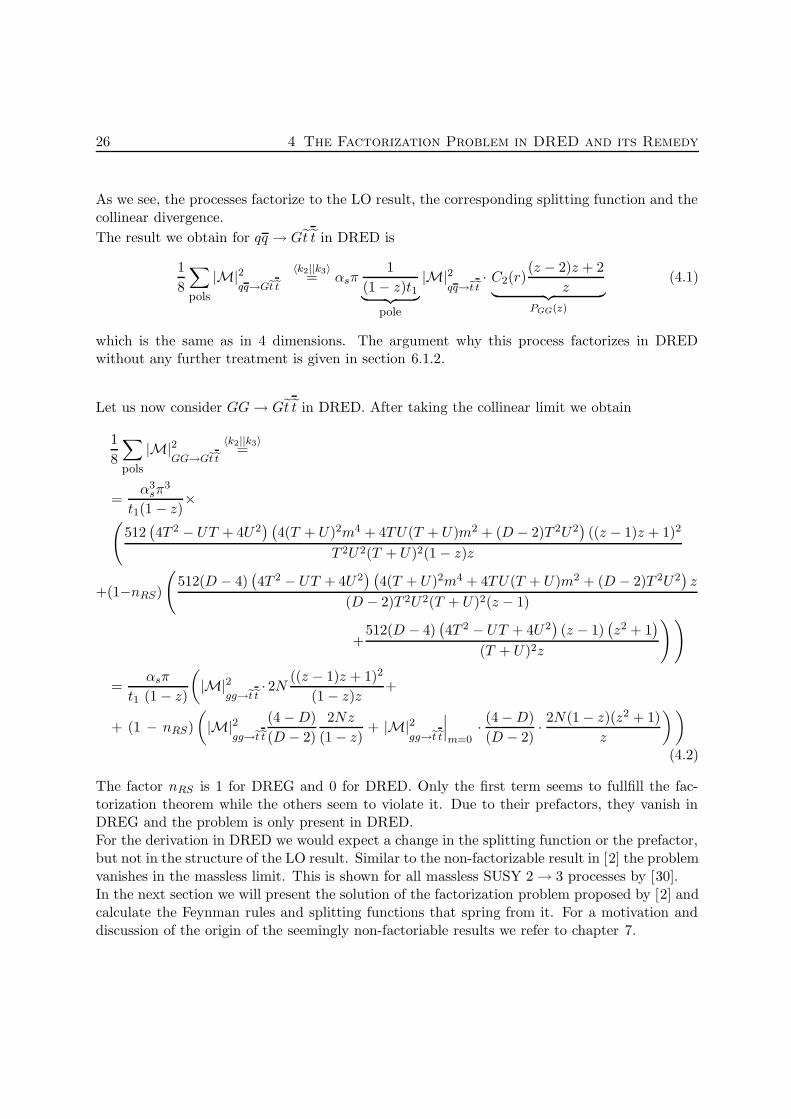
4.1 Real NLO Corrections and non-Factorizable Terms
We consider hadroproduction of stops via gluon and quark fusion which are essential processesrelevant for an experimental confirmation of SUSY and for the determination of SUSY pa-rameters. While the process involving quarks factorizes in DRED as expected, we also findnon-factorizable terms for the stop production via gluon fusion, a process similar to the onefor which factorization has been found to fail before [1]. We solve the problem for this processfollowing the idea of Signer and Stockinger, who applied their solution [2] to the problem in [1].Using their approach, the factorization problem does not seem to be a shortcoming of DREDany longer.We will now investigate how the processes for stop production behave in DRED and in 4 di-mensions. The factorization of both processes in 4 dimensions can be performed as expected,for the calculation see sections 6.1.1 and 6.2.1:
1
8
∑
pols
|M|2qq→Get et
〈k2||k3〉= αsπ ·
1
(1 − z)t1︸ ︷︷ ︸pole
|M|2qq→et et
· C2(r)(z − 2)z + 2
z︸ ︷︷ ︸PGq(z)
and
1
8
∑
pols
|M|2G G→Get et
〈k2||k3〉= αsπ · 1
(1 − z)t1︸ ︷︷ ︸pole
· |M|2GG→et et
2N((z − 1)z + 1)2
(z − 1)z︸ ︷︷ ︸PGG(z)
26 4 The Factorization Problem in DRED and its Remedy
As we see, the processes factorize to the LO result, the corresponding splitting function and thecollinear divergence.
The result we obtain for qq → Gt t in DRED is
1
8
∑
pols
|M|2qq→Get et
〈k2||k3〉= αsπ
1
(1 − z)t1︸ ︷︷ ︸pole
|M|2qq→et et
· C2(r)(z − 2)z + 2
z︸ ︷︷ ︸PGG(z)
(4.1)
which is the same as in 4 dimensions. The argument why this process factorizes in DREDwithout any further treatment is given in section 6.1.2.
Let us now consider GG→ Gt t in DRED. After taking the collinear limit we obtain
1
8
∑
pols
|M|2GG→Get et
〈k2||k3〉=
=α3
sπ3
t1(1 − z)×
(512
(4T 2 − UT + 4U 2
) (4(T + U)2m4 + 4TU(T + U)m2 + (D − 2)T 2U2
)((z − 1)z + 1)2
T 2U2(T + U)2(1 − z)z
+(1−nRS)
(512(D − 4)
(4T 2 − UT + 4U 2
) (4(T + U)2m4 + 4TU(T + U)m2 + (D − 2)T 2U2
)z
(D − 2)T 2U2(T + U)2(z − 1)
+512(D − 4)
(4T 2 − UT + 4U 2
)(z − 1)
(z2 + 1
)
(T + U)2z
))
=αsπ
t1 (1 − z)
(|M|2
gg→et et· 2N ((z − 1)z + 1)2
(1 − z)z+
+ (1 − nRS)
(|M|2
gg→et et
(4 −D)
(D − 2)
2Nz
(1 − z)+ |M|2
gg→et et
∣∣∣m=0
· (4 −D)
(D − 2)· 2N(1 − z)(z2 + 1)
z
))
(4.2)
The factor nRS is 1 for DREG and 0 for DRED. Only the first term seems to fullfill the fac-torization theorem while the others seem to violate it. Due to their prefactors, they vanish inDREG and the problem is only present in DRED.For the derivation in DRED we would expect a change in the splitting function or the prefactor,but not in the structure of the LO result. Similar to the non-factorizable result in [2] the problemvanishes in the massless limit. This is shown for all massless SUSY 2 → 3 processes by [30].In the next section we will present the solution of the factorization problem proposed by [2] andcalculate the Feynman rules and splitting functions that spring from it. For a motivation anddiscussion of the origin of the seemingly non-factoriable results we refer to chapter 7.
4.2 Remedy: The ε Scalar 27
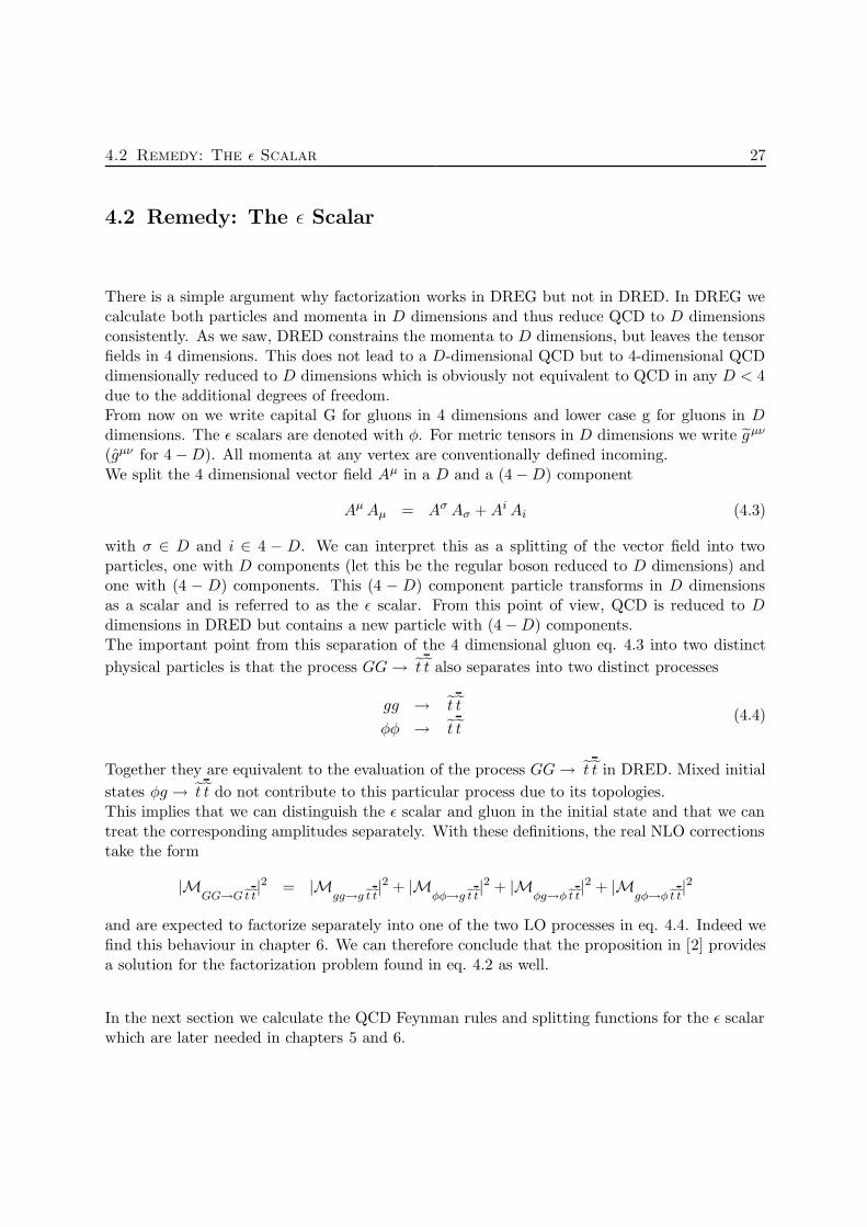
4.2 Remedy: The ε Scalar
There is a simple argument why factorization works in DREG but not in DRED. In DREG wecalculate both particles and momenta in D dimensions and thus reduce QCD to D dimensionsconsistently. As we saw, DRED constrains the momenta to D dimensions, but leaves the tensorfields in 4 dimensions. This does not lead to a D-dimensional QCD but to 4-dimensional QCDdimensionally reduced to D dimensions which is obviously not equivalent to QCD in any D < 4due to the additional degrees of freedom.From now on we write capital G for gluons in 4 dimensions and lower case g for gluons in Ddimensions. The ε scalars are denoted with φ. For metric tensors in D dimensions we write gµν
(gµν for 4 −D). All momenta at any vertex are conventionally defined incoming.We split the 4 dimensional vector field Aµ in a D and a (4 −D) component
AµAµ = Aσ Aσ +AiAi (4.3)
with σ ∈ D and i ∈ 4 − D. We can interpret this as a splitting of the vector field into twoparticles, one with D components (let this be the regular boson reduced to D dimensions) andone with (4 − D) components. This (4 − D) component particle transforms in D dimensionsas a scalar and is referred to as the ε scalar. From this point of view, QCD is reduced to Ddimensions in DRED but contains a new particle with (4 −D) components.The important point from this separation of the 4 dimensional gluon eq. 4.3 into two distinct
physical particles is that the process GG→ t t also separates into two distinct processes
gg → t t
φφ → t t(4.4)
Together they are equivalent to the evaluation of the process GG→ t t in DRED. Mixed initial
states φg → t t do not contribute to this particular process due to its topologies.This implies that we can distinguish the ε scalar and gluon in the initial state and that we cantreat the corresponding amplitudes separately. With these definitions, the real NLO correctionstake the form
|MGG→G et et
|2 = |Mgg→g et et
|2 + |Mφφ→g et et
|2 + |Mφg→φ et et
|2 + |Mgφ→φ et et
|2
and are expected to factorize separately into one of the two LO processes in eq. 4.4. Indeed wefind this behaviour in chapter 6. We can therefore conclude that the proposition in [2] providesa solution for the factorization problem found in eq. 4.2 as well.
In the next section we calculate the QCD Feynman rules and splitting functions for the ε scalarwhich are later needed in chapters 5 and 6.

28 4 The Factorization Problem in DRED and its Remedy
4.3 Feynman Rules for the ε Scalar
To perform the actual calculations in DRED, we will first derive the Feynman rules from theQCD Lagrangian. We start with the 4-dimensional Lagrangian for QCD dimensionally reducedto D dimensions, and split the fields Aµ into their D and (4−D) component parts. We directlyobtain the Lagrangian in terms of the the D dimensional gluon and the ε scalar. Starting fromthis we derive the Feynman rules for these particles.Let us consider the QCD Lagrangian coupled to a complex scalar (which will be identified witha stop)
LQCD,S = −1
4F a
µνFµν a + (Dµφ)†(Dµφ) −m2φ2 + ψ(i /D −mf )ψ (4.5)
We insert the covariant derivative and the field strength F
F aµν = ∂µA
aν − ∂νA
aµ + gsf
abcAbµA
cν
Dµ = ∂µ − igsAaµt
a
where fabc are the structure constants of the gauge group. We substitute the field strength intothe pure gauge part − 1
4FaµνF
µν a
− 1
4F a
µνFµν a = −1
4(∂µA
aν − ∂νA
aµ + gsf
abcAbµA
cν)(∂
µAν a − ∂νAµ a + gsfaefAµ eAνf )
= −1
4(∂µA
aν∂µA
ν,a − ∂µAaν∂
νAµ,a + ∂µAaνgsf
aefAµ eAν f
︸ ︷︷ ︸∗
− ∂νAaµ∂µA
ν,a + ∂νAaµ∂
νAµ,a − ∂νAaµgsf
aefAµ eAν f
︸ ︷︷ ︸∗
+ gsfabcAb
µAcν∂
µAν a
︸ ︷︷ ︸∗
− gsfabcAb
µAcν∂
νAµ a
︸ ︷︷ ︸∗
+ g2sf
abcAbµA
cνf
aefAµ eAν f
︸ ︷︷ ︸∗
) (4.6)
The parts from which we evaluate the Feynman rules for the vertices used here are marked with∗. We now split the 4 dimensional vector fields with indices µ , ν into D dimensions (marked byρ , σ) and (4 −D) dimensions (marked by i, j):
AµAµ → AρA
ρ +AjAj
∂µAµ → ∂ρA
ρ + ∂jAj
︸ ︷︷ ︸0
(4.7)
The last term with the derivative in (4 − D) dimensions does not exist as the momenta onlyhave components in D dimensions.
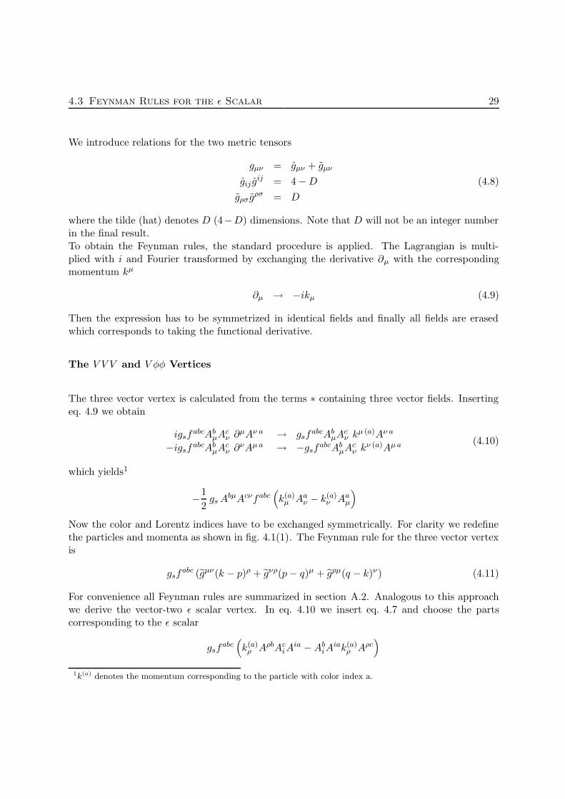
4.3 Feynman Rules for the ε Scalar 29
We introduce relations for the two metric tensors
gµν = gµν + gµν
gij gij = 4 −D (4.8)
gρσ gρσ = D
where the tilde (hat) denotes D (4−D) dimensions. Note that D will not be an integer numberin the final result.To obtain the Feynman rules, the standard procedure is applied. The Lagrangian is multi-plied with i and Fourier transformed by exchanging the derivative ∂µ with the correspondingmomentum kµ
∂µ → −ikµ (4.9)
Then the expression has to be symmetrized in identical fields and finally all fields are erasedwhich corresponds to taking the functional derivative.
The V V V and V φφ Vertices
The three vector vertex is calculated from the terms ∗ containing three vector fields. Insertingeq. 4.9 we obtain
igsfabcAb
µAcν ∂
µAν a → gsfabcAb
µAcν k
µ (a)Aν a
−igsfabcAb
µAcν ∂
νAµ a → −gsfabcAb
µAcν k
ν (a)Aµ a (4.10)
which yields1
−1
2gsA
bµAcνfabc(k(a)
µ Aaν − k(a)
ν Aaµ
)
Now the color and Lorentz indices have to be exchanged symmetrically. For clarity we redefinethe particles and momenta as shown in fig. 4.1(1). The Feynman rule for the three vector vertexis
gsfabc (gµν(k − p)ρ + gνρ(p− q)µ + gρµ(q − k)ν) (4.11)
For convenience all Feynman rules are summarized in section A.2. Analogous to this approachwe derive the vector-two ε scalar vertex. In eq. 4.10 we insert eq. 4.7 and choose the partscorresponding to the ε scalar
gsfabc(k(a)
ρ AρbAciA
ia −AbiA
iak(a)ρ Aρc
)
1k(a) denotes the momentum corresponding to the particle with color index a.

30 4 The Factorization Problem in DRED and its Remedy
p
q
kb
c
a
(1)c
a
d
b
(2)
Figure 4.1: Denotation of the momenta, color indices and Lorentz indices. The arrows markthe direction of the momentum.
After symmetrizing in a and c we find the Feynman rule for the vector-two ε scalar vertex
gρ
φi
φj
gs (q − k)ρ gijfabc (4.12)
The same result is achieved by removing all terms in eq. 4.11 with metric tensors mixing D and(4 −D)-dimensional indices.
The V V V V , V V φφ and φφφφ Vertices
The 4-vector vertex is calculated from the part of the Lagrangian
g2sf
abcAbµA
cνf
aefAµ eAν f
by decomposing the expression AµAµ with eqs. 4.7. For the D-dimensional component we
obtain the result−ig2
s
(fabef cde (gµρgνσ − gµσ gνρ)
+facef bde (gµν gρσ − gµσ gνρ)+ fadef bce (gµν gρσ − gµρgνσ)
) (4.13)
Analogous we evaluate the 2-vector 2-ε scalar coupling
4.3 Feynman Rules for the ε Scalar 31
φi
φj
gρ
gσ
−ig2sf
abef cdegij gρσ (4.14)
Additionally there is a four scalar vertex including only ε scalars:
φi
φj
φk
φl
−ig2s
(fabef cde
(gij gkl − gjkgil
)
+facef bde(gjlgik − gjkgli
)
+ fadef bce(gjlgik − gij glk
)) (4.15)
The FFV and FFφ Vertices
The vertex for the coupling of two fermions and a vector boson is
igsγρta
where γρ is a Dirac matrix. The γ matrices are defined such that
{γµ, γν} = 2gµν (4.16a)
{γρ, γσ} = 2gρσ (4.16b)
{γi, γj} = 2gij (4.16c)
{γi, γρ} = 0 (4.16d)
The ε scalar two-fermion vertex is derived as
φi
q
q
igsγita (4.17)
32 4 The Factorization Problem in DRED and its Remedy
The trace identities for these γ matrices can be found in A.1.
The V V F F and F F φφ Vertices
The procedure to obtain the Feynman rules is the same as before. First, the 4-dimensional fieldsare split in 4 and (4−D) components, then we symmetrize and Fourier transform iL and eraseall external fields. The couplings of vector bosons and squarks are derived from
(Dµφ)†(Dµφ) =((∂µ − igsA
bµt
b)φ)†
(∂µ − igsAµ ata)φ
which is part of the Lagrangian in eq. 4.5. After symmetrizing color and Lorentz indices, theFeynman rule for the vector-two scalar (squarks) coupling is
ig2s{ta, tc}gµν (4.18)
For the ε scalar the procedure is analogous and we obtain
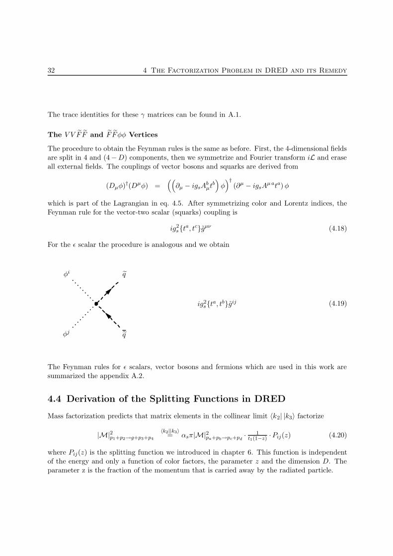
φj
φi
q
q
ig2s{ta, tb}gij (4.19)
The Feynman rules for ε scalars, vector bosons and fermions which are used in this work aresummarized the appendix A.2.
4.4 Derivation of the Splitting Functions in DRED
Mass factorization predicts that matrix elements in the collinear limit 〈k2| |k3〉 factorize
|M|2p1+p2→g+p3+p4
〈k2||k3〉= αsπ|M|2pa+pb→pc+pd
· 1t1(1−z) ·Pij(z) (4.20)
where Pij(z) is the splitting function we introduced in chapter 6. This function is independentof the energy and only a function of color factors, the parameter z and the dimension D. Theparameter z is the fraction of the momentum that is carried away by the radiated particle.

4.4 Derivation of the Splitting Functions in DRED 33
The splitting functions can be derived from common three particle vertices by setting two par-ticles collinear. We derive the splitting function using the definition
Pij(z) =z(1 − z)
2k2⊥
∑
pols
|Mi−>jf |2 (4.21)
where j is the collinear particle and i the inital particle radiating j [23]. These functions areknown for standard splittings such as
q → q GG→ GG
(4.22)
and can be found in [23] for 4 dimensions.Since we treat the ε scalars from the last section as partons of their own, new splitting functionshave to be evaluated
q → φ qg → φφφ→ φ gφ→ g φ
(4.23)
We derive these six splitting functions in the following in D dimensions to confirm the results inchapter 6. The momenta for the following vertices are defined incoming for the initial particlesand outbound for the particles in the final state. For simplicity the coupling constant gs isomitted in this section.As mentioned in section 2.2 there are at least two ways to derive splitting functions. In section2.2 we guarantee momentum conservation by the parametrization of the collinear momentumwith eqs. 2.5 and the momenta as they appear in fig. 4.2. Thus the particle with momentumkc = ka − kb is offshell with k2
⊥/z. This approach is similar to [20]. The crucial point is thatfor offshell particles, we can not use the polarization sum as in eq. A.13. Therefore the particlewhich enters the partonic process is kept offshell but is seen as a propagating particle (whichis acceptable since they are always offshell). This propagator can then be absorbed into thepartonic process as done in section 2.2.To avoid the use of a partonic process, we violate momentum conservation in order to keep allthree particles onshell. This has the advantage that we can use the polarization sum eq. A.13. Acomparison, e.g. with the derivation in 2.2 shows that both approaches lead to the same results.
Splitting Function for q → gq
Consider a quark a with momentum ka which emits a gluon b with momentum kb. We areinterested in the vertex structure of this process where the quark a emits the gluon collinearly
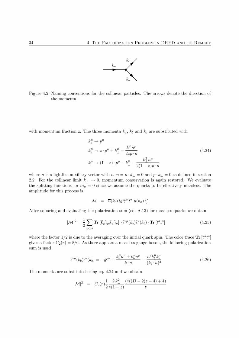
34 4 The Factorization Problem in DRED and its Remedy
ka
kb
kc
Figure 4.2: Naming conventions for the collinear particles. The arrows denote the direction ofthe momenta.
with momentum fraction z. The three momenta ka, kb and kc are substituted with
kµa → pµ
kµb → z · pµ + kµ
⊥ − k2⊥n
µ
2zp ·n (4.24)
kµc → (1 − z) · pµ − kµ
⊥ − k2⊥n
µ
2(1 − z)p ·n
where n is a lightlike auxiliary vector with n ·n = n · k⊥ = 0 and p · k⊥ = 0 as defined in section2.2. For the collinear limit k⊥ → 0, momentum conservation is again restored. We evaluatethe splitting functions for mq = 0 since we assume the quarks to be effectively massless. Theamplitude for this process is
M = u(kc) ig γµ ta u(ka) ε
∗µ
After squaring and evaluating the polarization sum (eq. A.13) for massless quarks we obtain
|M|2 =1
2
∑
pols
Tr [/kcγµ/kaγν ] · ε∗µ(kb)εν(kb) ·Tr [tata] (4.25)
where the factor 1/2 is due to the averaging over the initial quark spin. The color trace Tr [tata]gives a factor C2(r) = 8/6. As there appears a massless gauge boson, the following polarizationsum is used
ε∗µ(kb)εν(kb) = −gµν +
kµb n
ν + kνb n
µ
k ·n − n2kµb k
νb
(kb ·n)2(4.26)
The momenta are substituted using eq. 4.24 and we obtain
|M|2 = C2(r)1
2
2 k2⊥
z(1 − z)
(z((D − 2)z − 4) + 4)
z

4.4 Derivation of the Splitting Functions in DRED 35
which gives for D = 4
|M|2 = C2(r) ·z2 − 2z + 2
(z − 1)z2· 2 k2
⊥z(1 − z)
where (z(1 − z))/(2k2⊥) represents the collinear pole of the process. The splitting function is a
function of z, the dimension and a color factor
g
ka → p
kb → zp
kc → (1 − z)pPgq =
C2(r)12 ·
(z((D−2)z−4)+4)z
D→4=
PGq = C2(r) · 1+(1−z)2
z
(4.27)
Splitting Function for q → φq
For the calculation in dimensional reduction we need the splitting function for q → φq. Thefunction is calculated in the same way as in the last section with respect to the ε scalar. Theamplitude for this process is the same as eq. 4.25 except for the (4 − D) dimensional Lorentzindex of the Dirac matrices and the (4 − D) dimensional polarization vectors. Analogous toeq. 4.25 one derives
|M|2 =1
2
∑
pols
Tr [/kcγµ/kaγν ] · ε∗µ(kb)εν(kb) ·Tr [tata]
The polarization sum of the ε scalars has the simple form
ε∗µ(kb)εν(kb) = −gµν (4.28)
Since the momenta are still in D dimensions, they do not appear in this polarization sum as ineq. 4.26. Due to these changes we derive
|M|2 =1
2
∑
pols
Cs(r) ·2(4 −D)
(z − 1)· k2
⊥
= 2C2(r)1
2
2 k2⊥
z(1 − z)· z(4 −D)
with eq. 4.21 the last expression yields the splitting function
36 4 The Factorization Problem in DRED and its Remedy
φ
ka → p
kb → zp
kc → (1 − z)p
Pφq = 12C2(r)(4 −D)z (4.29)
Pφq and Pgq together give the 4 dimensional splitting function PGq.
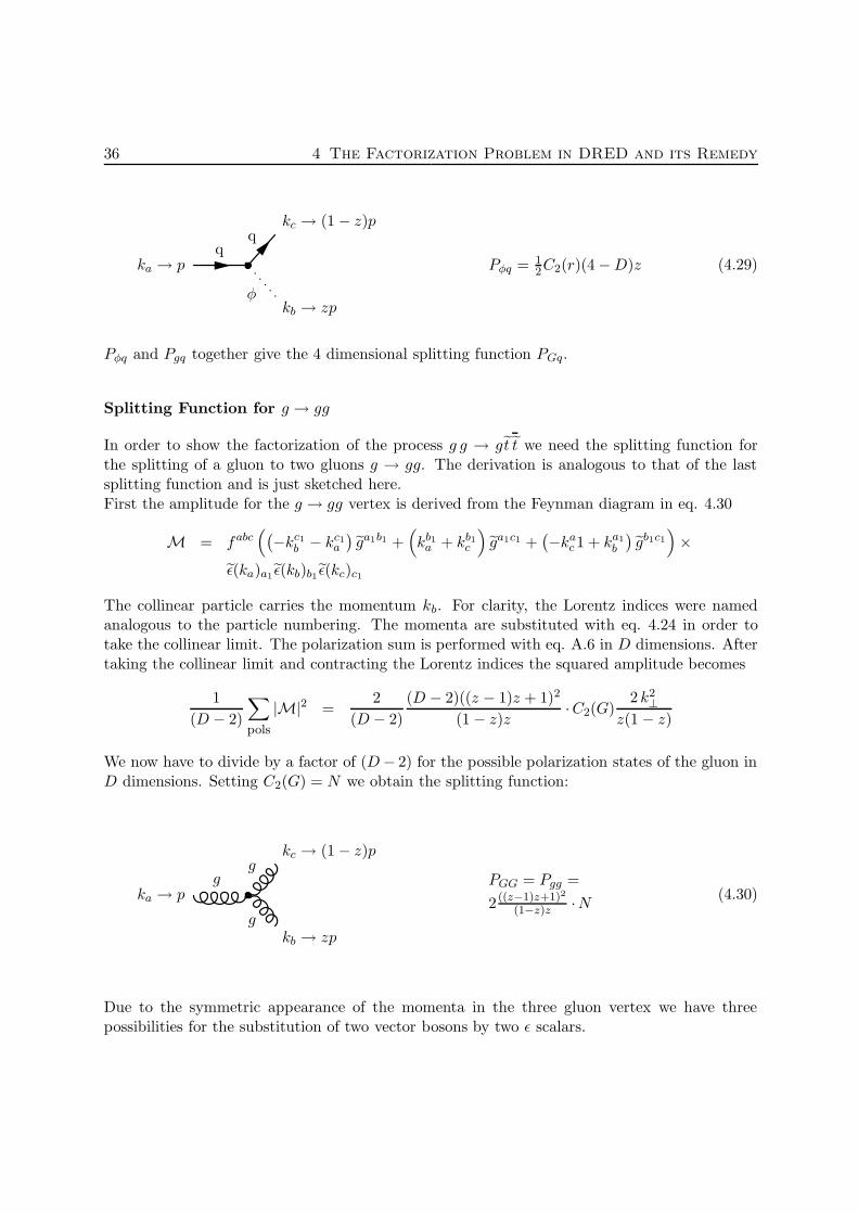
Splitting Function for g → gg
In order to show the factorization of the process g g → gt t we need the splitting function forthe splitting of a gluon to two gluons g → gg. The derivation is analogous to that of the lastsplitting function and is just sketched here.First the amplitude for the g → gg vertex is derived from the Feynman diagram in eq. 4.30
M = fabc((
−kc1b − kc1
a
)ga1b1 +
(kb1
a + kb1c
)ga1c1 +
(−ka
c1 + ka1b
)gb1c1
)×
ε(ka)a1 ε(kb)b1 ε(kc)c1
The collinear particle carries the momentum kb. For clarity, the Lorentz indices were namedanalogous to the particle numbering. The momenta are substituted with eq. 4.24 in order totake the collinear limit. The polarization sum is performed with eq. A.6 in D dimensions. Aftertaking the collinear limit and contracting the Lorentz indices the squared amplitude becomes
1
(D − 2)
∑
pols
|M|2 =2
(D − 2)
(D − 2)((z − 1)z + 1)2
(1 − z)z·C2(G)
2 k2⊥
z(1 − z)
We now have to divide by a factor of (D− 2) for the possible polarization states of the gluon inD dimensions. Setting C2(G) = N we obtain the splitting function:
g
g
g
ka → p
kb → zp
kc → (1 − z)p
PGG = Pgg =
2 ((z−1)z+1)2
(1−z)z ·N (4.30)
Due to the symmetric appearance of the momenta in the three gluon vertex we have threepossibilities for the substitution of two vector bosons by two ε scalars.
4.4 Derivation of the Splitting Functions in DRED 37
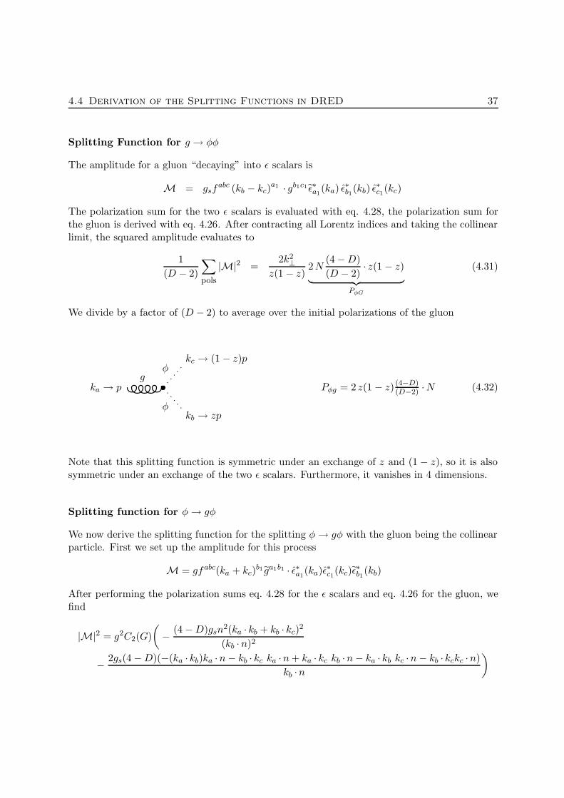
Splitting Function for g → φφ
The amplitude for a gluon “decaying” into ε scalars is
M = gsfabc (kb − kc)
a1 · gb1c1 ε∗a1(ka) ε
∗b1
(kb) ε∗c1
(kc)
The polarization sum for the two ε scalars is evaluated with eq. 4.28, the polarization sum forthe gluon is derived with eq. 4.26. After contracting all Lorentz indices and taking the collinearlimit, the squared amplitude evaluates to
1
(D − 2)
∑
pols
|M|2 =2k2
⊥z(1 − z)
2N(4 −D)
(D − 2)· z(1 − z)
︸ ︷︷ ︸PφG
(4.31)
We divide by a factor of (D − 2) to average over the initial polarizations of the gluon
gφ
φ
ka → p
kb → zp
kc → (1 − z)p
Pφg = 2 z(1 − z) (4−D)(D−2) ·N (4.32)
Note that this splitting function is symmetric under an exchange of z and (1 − z), so it is alsosymmetric under an exchange of the two ε scalars. Furthermore, it vanishes in 4 dimensions.
Splitting function for φ→ gφ
We now derive the splitting function for the splitting φ→ gφ with the gluon being the collinearparticle. First we set up the amplitude for this process
M = gfabc(ka + kc)b1 ga1b1 · ε∗a1
(ka)ε∗c1
(kc)ε∗b1
(kb)
After performing the polarization sums eq. 4.28 for the ε scalars and eq. 4.26 for the gluon, wefind
|M|2 = g2C2(G)
(− (4 −D)gsn
2(ka · kb + kb · kc)2
(kb ·n)2
− 2gs(4 −D)(−(ka · kb)ka ·n− kb · kc ka ·n+ ka · kc kb ·n− ka · kb kc ·n− kb · kckc ·n)
kb ·n
)

38 4 The Factorization Problem in DRED and its Remedy
The collinear limit is taken with the substitution in eq. 4.24. After evaluating the color sum onefinds
1
4 −D
∑
pols
|M|2 = g2 2k2⊥
(1 − z)zC2(G)
(1 − z)
z
As the incoming particle is an ε scalar we have to divide by a factor of (4 −D). The splittingfunction is then
φ
g
φ
ka → p
kb → zp
kc → (1 − z)p
Pgφ = 2 (1−z)z
·N (4.33)
The next splitting function can be derived from this one by an exchange of of z and (1 − z).
Splitting Function for φ→ φg
The last splitting function which is important for this work is the emission of a gluon by an εscalar as before but with the collinear particle being the ε scalar.The approach is analogous to the calculation above and the result is symmetric in an exchange ofthe the momenta kb and kc. After replacing the momenta as in eq. 4.24, the squared amplitudeis
1
(4 −D)
∑
pols
|M|2 = g2 1
k2⊥(1 − z)z
C2(G)z
(1 − z)
The factor (4 −D) cancels and we find for the splitting function
φ
φ
g
kb → p
kc → zp
ka → (1 − z)p
Pφφ = 2 z(1−z) ·N (4.34)
Note that only for the splitting of g → φφ the splitting function has a dimensional dependenceand vanishes for D → 4. The others still give a contribution in 4 dimensions.

4.4 Derivation of the Splitting Functions in DRED 39
As we have now derived the splitting functions, we know what to expect after the factorization ofboth processes investigated in this work (eqs. 1.2) and we will be able to see if the interpretationof the ε scalar as a parton of its own solves the factorization problem for these cases. We willstart with the calculation of the LO processes in DRED and then proceed to the real NLOprocesses and their factorization.
5 The 2 → 2 Case
As an introduction into DRED we calculate both processes eq. 1.2 in LO and show how the εscalars are implemented in the calculation. Both results are needed in chapter 6 since there wewill calculate real NLO corrections to these processes and perform the mass factorization.
5.1 Stop Production via Quark Fusion: qq → t t
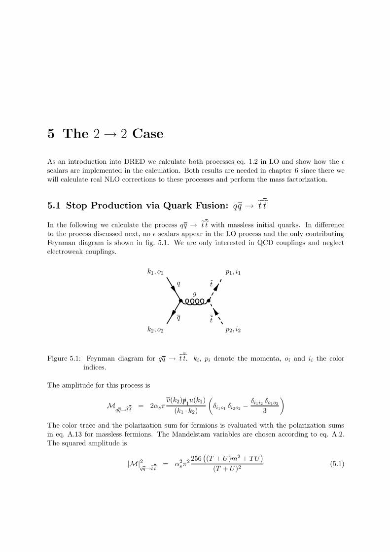
In the following we calculate the process qq → t t with massless initial quarks. In differenceto the process discussed next, no ε scalars appear in the LO process and the only contributingFeynman diagram is shown in fig. 5.1. We are only interested in QCD couplings and neglectelectroweak couplings.
q
tq
gt
k2, o2
k1, o1
p2, i2
p1, i1
Figure 5.1: Feynman diagram for qq → t t. ki, pi denote the momenta, oi and ii the colorindices.
The amplitude for this process is
Mqq→et et
= 2αsπv(k2)/p1
u(k1)
(k1 · k2)
(δi1o1 δi2o2 −
δi1i2 δo1o2
3
)
The color trace and the polarization sum for fermions is evaluated with the polarization sumsin eq. A.13 for massless fermions. The Mandelstam variables are chosen according to eq. A.2.The squared amplitude is
|M|2qq→et et
= α2sπ
2 256((T + U)m2 + TU
)
(T + U)2(5.1)

5.2 Stop Production via Gluon Fusion: GG → t t 41
where m denotes the stop mass. In difference to the example in section 5.2 this squared am-plitude lacks any dimensional dependence, which is due to the absence of external vector bosons.
The result is equal to [29]1. The result from eq. 5.1 is not yet averaged over polarizationstates and colors. After averaging we get
1
9 · 4 |M|2qq→et et
= α2sπ
2 1
9
64((T + U)m2 + TU
)
(T + U)2
This result is given for completeness, but in further calculations we will always refer to theunaveraged result in eq. 5.1.
5.2 Stop Production via Gluon Fusion: GG → t t
Now we look at the stop production via gluon fusion in LO. To simplify the calculation, weperform it with an unphysical polarization sum and subtract the unphysical states via externalBRST ghosts.The Feynman rules needed have been derived in chapter 4.3 and are summarized in the appendix
A.2. The Feynman diagrams for the LO gg → t t are shown in fig. 5.2, those for the ghostprocesses in fig. 5.3.We calculate the amplitudes for the D-dimensional gluon g and the ε scalar (φ) separately.
Therefore we consider the process gg → t t and φφ → t t 2. Since the calculation is performedin DRED with particles and momenta in D dimensions, we have to derive the process wherethe gluon is substituted by the ε scalar as shown in fig. 5.4. The color indices and momenta are
defined as they appear in fig. 5.2(1). The amplitudes for the g g → t t are
M1 =(ta tb − tb ta
)ij
2αsπ
(k1 · k2)×
(εa(k1) · k2 εb(k2) · (k2) + 2εa(k1) · p1(2ε
b(k2) · k1 + εb(k2) · k2)−
−4εa(k1) · k2 εb(k2) · p1 − (εa(k1) · k1)(εb(k2) · k1 + 2εb(k2) · p1)−
−2εa(k1) · εb(k2) k1 · p1 + 2εa(k1) · εb(k2) k2 · p1
)
M2 =2αsπ (ta tb)ij
(k1 · p1)· ((εa(k1) · k1) − 2(εa(k1) · p1)) ×
(2(εb(k2) · k1) + (εb(k2) · k2) − 2(εb(k2), p1))
M3 = 4αsπ(ta tb + tbta
)ij
(εa(k1) · εb(k2)
)
1There is a relative factor of two since we take only one type of stop into account.2LO processes with a gluon and an ε scalar are also possible, but are not present in this process.

42 5 The 2 → 2 Case
M4 =2αsπ (tb ta)ij
(k1 · p2)×
(εa(k1) · k1 + 2εa(k1) · k2 − 2(εa(k1) · p1)(εb(k2) · k2 − 2(εb(k2) · p1))
The polarization sum is evaluated with eq. A.7 in D dimensions. After evaluating the colortrace, we derive the squared matrix element
|M|2g g→et et,unphys.
= α2sπ
2
(4096m4
3U2+
32(128m4 + 128Tm2 + 32DT 2 − 55T 2
)
3T 2
+1024
(4m2T −m4
)
3TU− 384
(8m2 + 2DT − 3T
)
T + U+
384(2DT 2 − 3T 2
)
(T + U)2
)
where m ist the stop mass. Due to the use of the unphysical polarization sum, BRST ghosts haveto be subtracted after squaring both amplitudes. The Feynman graphs for the BRST ghosts areshown in fig. 5.3 and the corresponding amplitudes are
M1,η η→et et
=2αsπ
(tatb − tbta
)ij
(k1 · k2 − 2k1 · p1)
k1 · k2
M2,η η→et et
=2αsπ
(tatb − tbta
)ij
(k1 · k2 − 2k2 · p1)
k1 · k2
After evaluating the color trace, the squared amplitude is
|M|2ηη→et et
= |M|2ηη→et et
= α2sπ
2 48(T − U)2
(T + U)2
Now we perform the calculation for the process including the ε scalar. Due to the topology ofvertices for the vector-scalar coupling, there is always an even number of ε scalars. The Feynmangraphs for the processes including ε scalars are shown in fig. 5.4.The amplitudes are calculated with the help of the Feynman rules from section 4.3:
M1,φ = −4αsπ
(tatb − tbta
)ijεa(k1) · εb(k2)(k1 · p1 − k2 · p1)
k1 · k2
M2,φ = 4αsπ(tatb + tbta
)ijεa(k1) · εb(k2)
The polarization sum for the ε scalars is evaluated with eq. A.8. The polarization vectors ε(k1)and ε(k2) are (4 −D)-dimensional and therefore give a (4 −D)-dimensional metric tensor gµν .

5.2 Stop Production via Gluon Fusion: GG → t t 43
g
tg
gt
k2, b
k1, a
p2, j
p1, i
(1)
g
t
t
g
t
k2
k1
p2
p1
(2)
g
t
t
g
k2
k1
p2
p1
(3)
g
tt
g
t
k2
k1
p2
p1
(4)
Figure 5.2: Feynman diagrams for gg → t t. The amplitudes are named analogous to thenumbering of the graphs. The first graph also gives the notation for the color indicesof the particles. The charge flow is indicated by the direction of the arrow at thescalar lines.
η
tη
gt
k2, b
k1, a
p2, j
p1, i
(1)
ηt
η
gt
k2
k1
p2
p1
(2)
Figure 5.3: Feynman diagrams for the BRST ghosts ηη → t t and ηη → t t.

44 5 The 2 → 2 Case
φ
tφ
gt
k2, b
k1, a
p2, j
p1, i
(1)
φ t
φ t
k2
k1
p2
p1
(2)
Figure 5.4: Feynman diagrams for φφ→ t t at LO.
After squaring the amplitudes we obtain terms of the form giving a dimensional dependence
|M1,φ + M2,φ|2 ∝ ε(k1)µε(k2)
µ · ε∗ν(k1)ε∗ν(k2)
∝ gµν gµν = (4 −D)
After calculating the color trace and sum over the polarization states, the squared amplitudesfor the ε scalars are
∑
pols
|M|2φφ→et et
= α2sπ
2 · 256(4 −D)(4T 2 − UT + 4U 2
)
3(T + U)2(5.2)
Since the ε scalars are formally seen as independent particles (see chapter 4), we need thisresult to show the NLO factorization in chapter 6. For D → 4 this matrix element vanishes asexpected.Now we can sum up the process including gluons and ghosts and derive the full matrix element
for gg → t t in D dimensions which is equal to the DREG result
∑
pols
|M|2g g, phys. =∑
pols
(|M|2g g, unphys. − |M|2ηη − |M|2ηη
)
= α2sπ
2 256(4T 2 − UT + 4U 2
) (4(T + U)2m4 + 4TU(T + U)m2 + (D − 2)T 2U2
)
3T 2U2(T + U)2(5.3)
To get the complete matrix element for the process gg → t t in DRED, the squared amplitudeincluding the ε scalars is added
1
2
∑
pols
|M|2GG→et et
=1
2
∑
pols
|M|2g g→et et, unphys.
+ |M|2φφ→et et
− 2|M|2ηη→et et
=1
2α2
sπ2 512
(4T 2 − UT + 4U 2
) (2(T + U)2m4 + 2TU(T + U)m2 + T 2U2
)
3T 2U2(T + U)2(5.4)
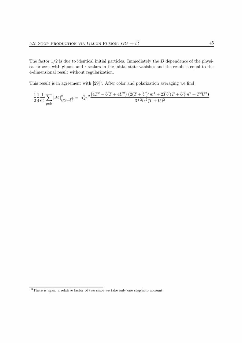
5.2 Stop Production via Gluon Fusion: GG → t t 45
The factor 1/2 is due to identical initial particles. Immediately the D dependence of the physi-cal process with gluons and ε scalars in the initial state vanishes and the result is equal to the4-dimensional result without regularization.
This result is in agreement with [29]3. After color and polarization averaging we find
1
2
1
4
1
64
∑
pols
|M|2GG→et et
= α2sπ
2
(4T 2 − UT + 4U 2
) (2(T + U)2m4 + 2TU(T + U)m2 + T 2U2
)
3T 2U2(T + U)2
3There is again a relative factor of two since we take only one stop into account.
6 Factorization of the Real NLO Processes
in DRED
The two most important channels for stop production at hadron colliders are
qq → t t
gg → t t(6.1)
In this chapter we will demonstrate that the real squared NLO amplitudes factorize in thecollinear limit in DRED if the method proposed in [2] is applied.After deriving the squared amplitude for the two LO processes in chapter 5 and calculating thesplitting functions for gluon-quark and gluon-gluon splitting and their corresponding splittingfunctions involving ε scalars in section 4.3 and 4.4, we now have the technical background toexplicitly calculate the collinear factorization for both processes in DRED.Both amplitudes are first factorized in 4 dimensions in order to show how the radiated gluonis made collinear and how to approach factorization. Then both calculations are performed inDRED. In the following we denote the 4 component gluon with capital G and the D-dimensionalgluon with lower case g. Without loss of generality we always consider the particle with mo-mentum k3 collinear to that with k2. If the momentum k3 is chosen collinear to k1 the approachis the same with respect to the pole 1/u1.
6.1 Stop Production via Quark Fusion: qq → G t t
We calculate the real NLO correction for stop production via quark fusion. Since mu,md � met
we consider the initial quarks to be massless. As discussed in chapter 2, massless particles in NLOcorrections lead to singularities if the emitted particle is collinear to the emitting particle. Thissingularity has to be handled by absorbing it into the PDFs. After separating the singularitywe are left with the LO process. Thus we expect that the squared matrix element of the realNLO correction in the collinear limit should have the form
|M|22→3〈k2||k3〉
= αsπ1
t1(1 − z)|M|22→2 ·P (z) (6.2)
where P(z) denotes the splitting function for the corresponding process derived in 4.4. Thesingularity is represented by 1/t1. The Mandelstam variable t1 is defined in eq. A.4.
We will first perform the calculation qq → G t t in 4 dimensions and demonstrate in detail howthe collinear limit is taken and how the factorization is obtained. After this, the factorization is
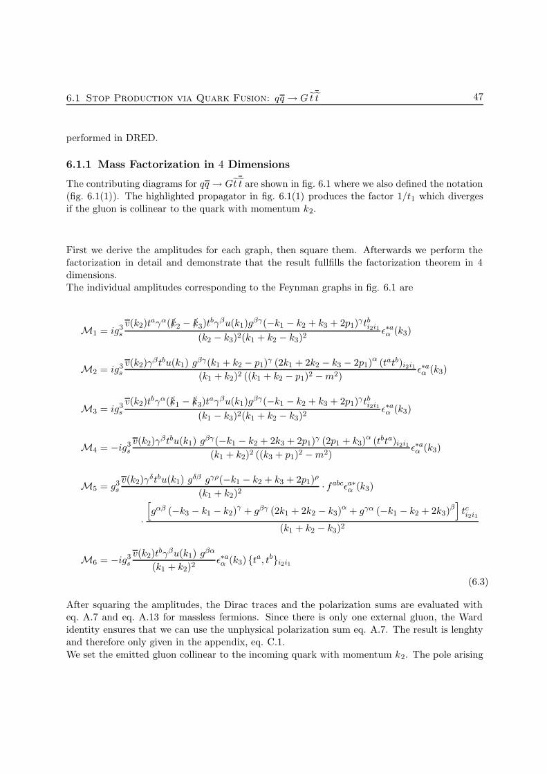
6.1 Stop Production via Quark Fusion: qq → G t t 47
performed in DRED.
6.1.1 Mass Factorization in 4 Dimensions
The contributing diagrams for qq → Gt t are shown in fig. 6.1 where we also defined the notation(fig. 6.1(1)). The highlighted propagator in fig. 6.1(1) produces the factor 1/t1 which divergesif the gluon is collinear to the quark with momentum k2.
First we derive the amplitudes for each graph, then square them. Afterwards we perform thefactorization in detail and demonstrate that the result fullfills the factorization theorem in 4dimensions.The individual amplitudes corresponding to the Feynman graphs in fig. 6.1 are
M1 = ig3s
v(k2)taγα(/k2 − /k3)t
bγβu(k1)gβγ(−k1 − k2 + k3 + 2p1)
γtbi2i1
(k2 − k3)2(k1 + k2 − k3)2ε∗aα (k3)
M2 = ig3s
v(k2)γβtbu(k1) g
βγ(k1 + k2 − p1)γ (2k1 + 2k2 − k3 − 2p1)
α (tatb)i2i1
(k1 + k2)2 ((k1 + k2 − p1)2 −m2)ε∗aα (k3)
M3 = ig3s
v(k2)tbγα(/k1 − /k3)t
aγβu(k1)gβγ(−k1 − k2 + k3 + 2p1)
γtbi2i1
(k1 − k3)2(k1 + k2 − k3)2ε∗aα (k3)
M4 = −ig3s
v(k2)γβtbu(k1) g
βγ(−k1 − k2 + 2k3 + 2p1)γ (2p1 + k3)
α (tbta)i2i1
(k1 + k2)2 ((k3 + p1)2 −m2)ε∗aα (k3)
M5 = g3s
v(k2)γδtbu(k1) g
δβ gγρ(−k1 − k2 + k3 + 2p1)ρ
(k1 + k2)2· fabcεa∗α (k3)
·
[gαβ (−k3 − k1 − k2)
γ + gβγ (2k1 + 2k2 − k3)α + gγα (−k1 − k2 + 2k3)
β]tci2i1
(k1 + k2 − k3)2
M6 = −ig3s
v(k2)tbγβu(k1) g
βα
(k1 + k2)2ε∗aα (k3) {ta, tb}i2i1
(6.3)
After squaring the amplitudes, the Dirac traces and the polarization sums are evaluated witheq. A.7 and eq. A.13 for massless fermions. Since there is only one external gluon, the Wardidentity ensures that we can use the unphysical polarization sum eq. A.7. The result is lenghtyand therefore only given in the appendix, eq. C.1.We set the emitted gluon collinear to the incoming quark with momentum k2. The pole arising

48 6 Factorization of the Real NLO Processes in DRED
k2, o2
k1, o1
p2, i2
p1, i1
k3, a(1)
k2
k1
p2
p1
k3
(2)
k2
k1
p2
p1
k3
(3) k2
k1
p2
p1
k3
(4)
k2
k1
p2
p1
k3
(5) k2
k1
p2
p1
k3
(6)
Figure 6.1: Feynman diagrams for the process qq → Gt t. k1 . . . k3 and p1, p2 denote the mo-menta of the particles. In this calculation, p2 is always substituted by the other fourmomenta via momentum conservation. The numbering corresponds to that of theamplitudes.
6.1 Stop Production via Quark Fusion: qq → G t t 49
from this momentum configuration appears in the squared amplitude as indicated (eq. 6.2).Based on the squared amplitude (eq. C.1) we will now give the detailed prescription how toperform the factorization:
• To simplify the expression, the pole leading to the collinear divergence is extracted bymultpliying the full expression eq. C.1 with (1 − z)(k2 − k3)
2 = (1 − z)t1.
• Since in these remaining terms no further pole 1/t1 appears, we can set k2 · k3 → 0.
• Now we implement the collinear limit for the gluon and the quarks by expressing themomentum of the emitted gluon in terms of the radiating quark momentum with
kµ3 → zkµ
2 + δkµ⊥ − δ2
(k⊥)2 nµ
2z k2 ·n(6.4)
For z = 0 the gluon is infinitely soft while for z = 1 it carries the total momentum ofthe incoming quark. Both k⊥ and n are needed to construct the collinear direction andguarantee momentum conservation. They are chosen as in eq. 2.5. A factor δ is introducedfor each k⊥ so that the expression can later be expanded in δ around 0. This approachensures that the order in k⊥ of each term is identified correctly.
• The squared amplitude (eq. C.1) with the substitution eq. 6.4 is expanded in δ around 0up to O(δ0). We have to check if terms depending on δ−1 or δ−2 appear. This is not thecase in this example but will be of importance later (section 6.2).
• The remaining expression depends on k1, k2, p1 and z
|M|2qq→G et et
〈k2||k3〉=
α3sπ
3
t1(1 − z)
(−(m2k1 · k2 − 2k1 · p1k2 · p1
)×
128((z − 1)
((z2 − 11z + 2
)k1 · k2 + 9(z − 2)(k1 · p1 − (z − 1)k2 · p1)
))
3 (zk1 · k2(k1 · p1 − (z − 1)k2 · p1)2)+O
(δ1))
• To compare this result with the LO result in eq. 5.1, we introduce kinetic variables definedin eq. A.2. However, since the particle with momentum k ′2 = (1 − z) · k2 enters the LOcross section, we need to redefine the Mandelstam variables according to fig. 6.2
k1 · k2 =S
2(1 − z)k1 · p1 = −T
2k2 · p1 = − U
2(1 − z)(6.5)
The relation S + T + U = 0 can still be used after this redefinition1.
1This relation is always correct after taking the collinear limit. Had we used this relation before the expansionaround δ, we would have neglected that the particle with momentum p′ is offshell implying a dependence ofS + T + U ∝ δ, δ2 6= 0. This relation will be derived in eq. 6.13.
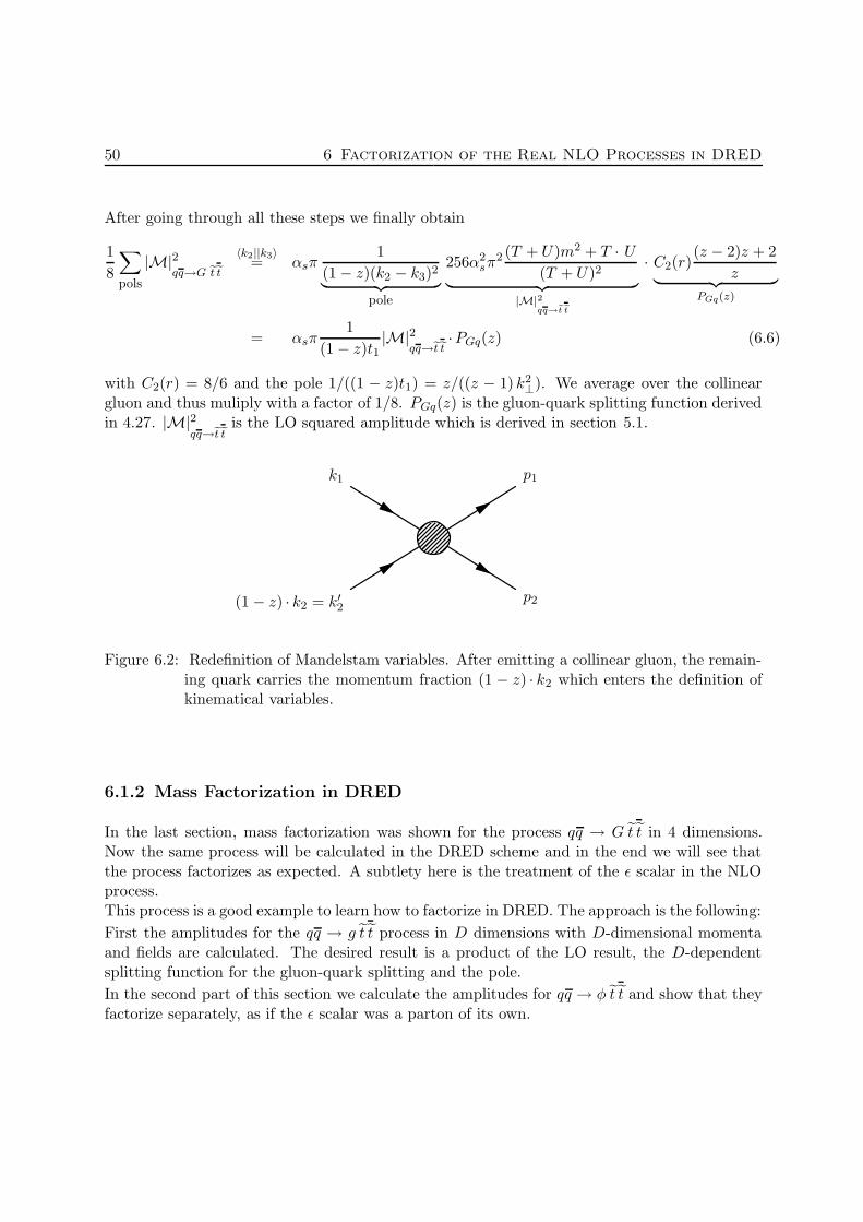
50 6 Factorization of the Real NLO Processes in DRED
After going through all these steps we finally obtain
1
8
∑
pols
|M|2qq→G et et
〈k2||k3〉= αsπ
1
(1 − z)(k2 − k3)2︸ ︷︷ ︸pole
256α2sπ
2 (T + U)m2 + T · U(T + U)2︸ ︷︷ ︸
|M|2qq→et et
· C2(r)(z − 2)z + 2
z︸ ︷︷ ︸PGq(z)
= αsπ1
(1 − z)t1|M|2
qq→et et·PGq(z) (6.6)
with C2(r) = 8/6 and the pole 1/((1 − z)t1) = z/((z − 1) k2⊥). We average over the collinear
gluon and thus muliply with a factor of 1/8. PGq(z) is the gluon-quark splitting function derivedin 4.27. |M|2
qq→et etis the LO squared amplitude which is derived in section 5.1.
(1 − z) · k2 = k′2
k1
p2
p1
Figure 6.2: Redefinition of Mandelstam variables. After emitting a collinear gluon, the remain-ing quark carries the momentum fraction (1 − z) · k2 which enters the definition ofkinematical variables.
6.1.2 Mass Factorization in DRED
In the last section, mass factorization was shown for the process qq → G t t in 4 dimensions.Now the same process will be calculated in the DRED scheme and in the end we will see thatthe process factorizes as expected. A subtlety here is the treatment of the ε scalar in the NLOprocess.This process is a good example to learn how to factorize in DRED. The approach is the following:
First the amplitudes for the qq → g t t process in D dimensions with D-dimensional momentaand fields are calculated. The desired result is a product of the LO result, the D-dependentsplitting function for the gluon-quark splitting and the pole.
In the second part of this section we calculate the amplitudes for qq → φ t t and show that theyfactorize separately, as if the ε scalar was a parton of its own.
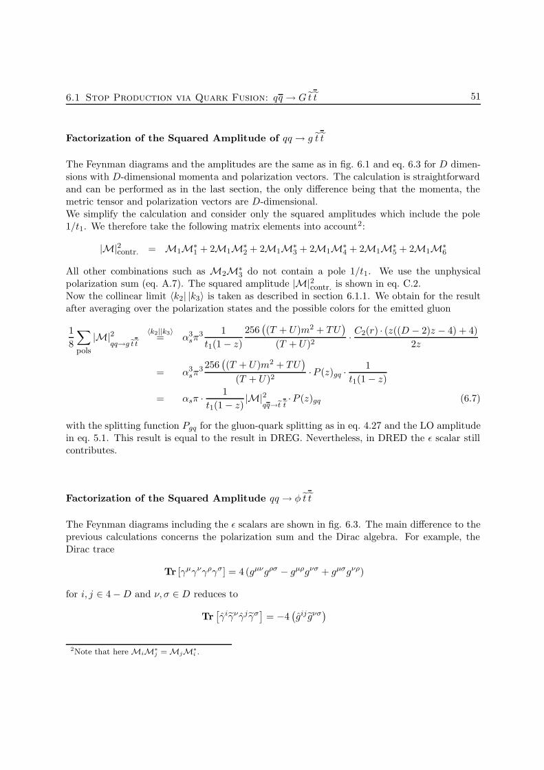
6.1 Stop Production via Quark Fusion: qq → G t t 51
Factorization of the Squared Amplitude of qq → g t t
The Feynman diagrams and the amplitudes are the same as in fig. 6.1 and eq. 6.3 for D dimen-sions with D-dimensional momenta and polarization vectors. The calculation is straightforwardand can be performed as in the last section, the only difference being that the momenta, themetric tensor and polarization vectors are D-dimensional.We simplify the calculation and consider only the squared amplitudes which include the pole1/t1. We therefore take the following matrix elements into account2:
|M|2contr. = M1M∗1 + 2M1M∗
2 + 2M1M∗3 + 2M1M∗
4 + 2M1M∗5 + 2M1M∗
6
All other combinations such as M2M∗3 do not contain a pole 1/t1. We use the unphysical
polarization sum (eq. A.7). The squared amplitude |M|2contr. is shown in eq. C.2.Now the collinear limit 〈k2| |k3〉 is taken as described in section 6.1.1. We obtain for the resultafter averaging over the polarization states and the possible colors for the emitted gluon
1
8
∑
pols
|M|2qq→g et et
〈k2||k3〉= α3
sπ3 1
t1(1 − z)
256((T + U)m2 + TU
)
(T + U)2· C2(r) · (z((D − 2)z − 4) + 4)
2z
= α3sπ
3 256((T + U)m2 + TU
)
(T + U)2·P (z)gq ·
1
t1(1 − z)
= αsπ ·1
t1(1 − z)|M|2
qq→et et·P (z)gq (6.7)
with the splitting function Pgq for the gluon-quark splitting as in eq. 4.27 and the LO amplitudein eq. 5.1. This result is equal to the result in DREG. Nevertheless, in DRED the ε scalar stillcontributes.
Factorization of the Squared Amplitude qq → φ t t
The Feynman diagrams including the ε scalars are shown in fig. 6.3. The main difference to theprevious calculations concerns the polarization sum and the Dirac algebra. For example, theDirac trace
Tr [γµγνγργσ] = 4 (gµνgρσ − gµρgνσ + gµσgνρ)
for i, j ∈ 4 −D and ν, σ ∈ D reduces to
Tr[γiγν γj γσ
]= −4
(gij gνσ
)
2Note that here MiM∗j = MjM
∗i .

52 6 Factorization of the Real NLO Processes in DRED
The individual amplitudes for the graphs in fig. 6.3 are
M1 = ig3s
v(k2)γjta (/k2 − /k3) γ
βtbu(k1)gβγ (−k1 − k2 + k3 + 2p1)
γ tbi2i1
(k2 − k3)2(k1 + k2 − k3)2ε(k3)
∗aj
M2 = −g3s
v(k2)tbγiu(k1) (−k3 − k1 − k2)
α gijfabcgαβ (−k1 − k2 + k3 + 2p1)β tci2i1
(k1 + k2)2(k1 + k2 − k3)2ε(k3)
∗aj
M3 = ig3s
v(k2)γβtb (/k1 − /k3) γ
jtau(k1)gβγ (−k1 − k2 + k3 + 2p1)
γ tbi2i1
(k1 − k3)2(k1 + k2 − k3)2ε(k3)
∗aj
M4 = ig3s
v(k2)γβtbu(k1)g
αβ
(k1 + k2)2{ta, tb}i2i1 ε(k3)
∗aj
where the hatted objects such as gµν or ε(k1) are in (4−D) dimensions and the tilded gµν in Ddimensions. The total result is shown in eq. C.3 with the Mandelstam definition from eq. A.4.After taking the collinear limit as in eq. 6.4 and applying the procedure as in section 6.1.1, thesquared amplitude in the collinear limit is
1
8
∑
pols
|M|2qq→φ et et
〈k2||k3〉= α3
sπ3 256
((T + U)m2 + TU
)
(T + U)21
t1(1 − z)· C2(r) · z(4 −D)
2
= α3sπ
3 256((T + U)m2 + TU
)
(T + U)2· 1
t1(1 − z)·P (z)φq
= αsπ1
t1(1 − z)|M|2
qq→et et·P (z)φq (6.8)
with the splitting function Pφq as in eq. 4.29.
Adding Both Amplitudes
We see that both processes factorize independently with different splitting functions. However,the same LO squared amplitude appears in both cases. This enables us to add both processes.The splitting functions for the D and (4−D) components then combine to give the 4 dimensionalsplitting function making this result equal to the unregularized one. This also implies that theD dependence cancels without taking the limit D → 4:
1
8
∑
pols
|M|2qq→G et et,DRED
〈k2||k3〉= α3
sπ3 256
((T + U)m2 + TU
)
(T + U)2· 1
t1(1 − z)· (Pφq + Pgq)
= α3sπ
3 256((T + U)m2 + TU
)
(T + U)2· 1
t1(1 − z)· ((z − 2)z + 2)
zC2(r)
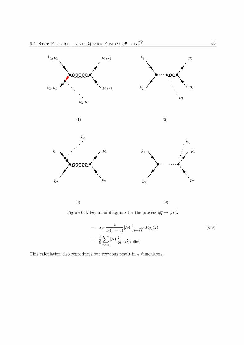
6.1 Stop Production via Quark Fusion: qq → G t t 53
k2, o2
k1, o1
p2, i2
p1, i1
k3, a
(1)
k2
k1
p2
p1
k3
(2)
k2
k1
p2
p1
k3
(3)
k2
k1
p2
p1
k3
(4)
Figure 6.3: Feynman diagrams for the process qq → φ t t.
= αsπ1
t1(1 − z)|M|2
qq→et et·PGq(z) (6.9)
=1
8
∑
pols
|M|2qq→et et, 4 dim.
This calculation also reproduces our previous result in 4 dimensions.
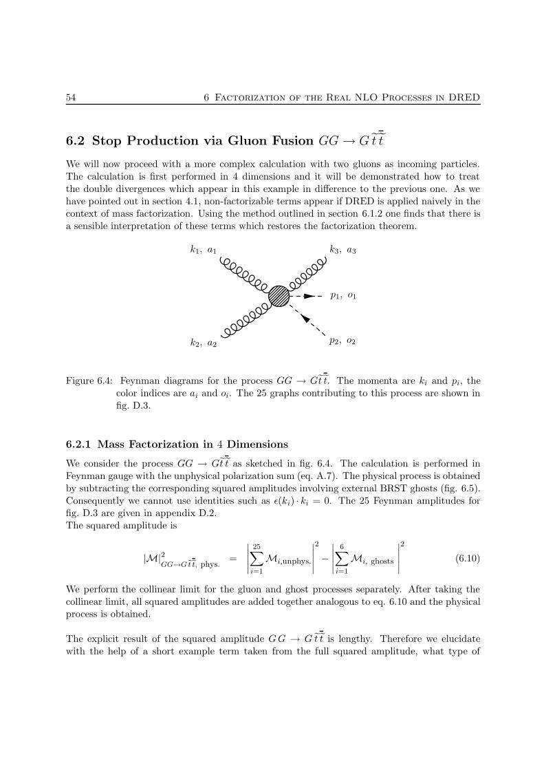
54 6 Factorization of the Real NLO Processes in DRED
6.2 Stop Production via Gluon Fusion GG → G t t
We will now proceed with a more complex calculation with two gluons as incoming particles.The calculation is first performed in 4 dimensions and it will be demonstrated how to treatthe double divergences which appear in this example in difference to the previous one. As wehave pointed out in section 4.1, non-factorizable terms appear if DRED is applied naively in thecontext of mass factorization. Using the method outlined in section 6.1.2 one finds that there isa sensible interpretation of these terms which restores the factorization theorem.
k2, a2
k1, a1
p2, o2
p1, o1
k3, a3
Figure 6.4: Feynman diagrams for the process GG → Gt t. The momenta are ki and pi, thecolor indices are ai and oi. The 25 graphs contributing to this process are shown infig. D.3.
6.2.1 Mass Factorization in 4 Dimensions
We consider the process GG → Gt t as sketched in fig. 6.4. The calculation is performed inFeynman gauge with the unphysical polarization sum (eq. A.7). The physical process is obtainedby subtracting the corresponding squared amplitudes involving external BRST ghosts (fig. 6.5).Consequently we cannot use identities such as ε(ki) · ki = 0. The 25 Feynman amplitudes forfig. D.3 are given in appendix D.2.The squared amplitude is
|M|2GG→G et et, phys.
=
∣∣∣∣∣
25∑
i=1
Mi,unphys.
∣∣∣∣∣
2
−∣∣∣∣∣
6∑
i=1
Mi, ghosts
∣∣∣∣∣
2
(6.10)
We perform the collinear limit for the gluon and ghost processes separately. After taking thecollinear limit, all squared amplitudes are added together analogous to eq. 6.10 and the physicalprocess is obtained.
The explicit result of the squared amplitude GG → G t t is lengthy. Therefore we elucidatewith the help of a short example term taken from the full squared amplitude, what type of
6.2 Stop Production via Gluon Fusion GG→ G t t 55
expressions arise and how to manage them.The difference and difficulty in this calculation in comparison to the process calculated in sec-tion 6.1 is that not only poles of order 1/(k2 − k3)
2 = 1/t1 appear, but also terms of order1/(k2 − k3)
4 = 1/t21. One of the divergences is treated as in the last chapter but the remainingone has to be dealt with separately. The key to remove it is to average over the azimuthaldirection of k⊥ which is unobservable in the collinear limit.We set the gluon with momentum k3 collinear to the one with momentum k2 by using theparametrization in eq. 6.4. The collinear divergence originates from the diagrams 5, 17, 18 and19 in fig. D.3 where the propagator goes onshell as k⊥ → 0.Our approach is the following: First the squared amplitudes are separated into parts dependingto 1/t1 and 1/t21. The other terms are ignored since they do not give a contribution to the result.The terms are very lengthy and are not shown. Before the collinear limit is performed, bothterms are combined.To show how the amplitude is factorized, we pick a convenient term from the full result con-taining a 1/t21 divergence and go through the calculation step by step. It is demonstrated howone of the two divergences vanishes after performing the azimuthal average. For this discussionwe express the pole 1/t21 as 1/(k2 · k3)
2, omitting all inessential factors for simplicity.We investigate
f (ki) =(k1 · k4 k2 · k3 − k1 · k3 k2 · k4 + k1 · k2k3 · k4)
2
(k2 · k3)2
One pole is extracted analogous to eq. 6.2. Therefore the term is multiplied with k2 · k3 andexpanded to make the structure more obvious
f (ki) · (k2 · k3) = k2 · k3(k1 · k4)2 − 2k1 · k3 k2 · k4 k1 · k4 + 2k1 · k2 k3 · k4k1 · k4
+(k1 · k3)
2(k2 · k4)2
k2 · k3+
(k1 · k2)2(k3 · k4)
2
k2 · k3− 2k1 · k2 k1 · k3 k2 · k4 k3 · k4
k2 · k3
Here terms of order (k2 · k3)1,(k2 · k3)
0 and (k2 · k3)−1 appear. In order to explain the vanishing
of these poles the collinear limit is parametrized using eq. 6.4. Since poles of the structure(kµ
⊥kν⊥)/k4
⊥ appear, introducing the variable δ helps to determine the order of the singularity.Here the gluons with k2 and k3 are onshell and we can conserve momentum by keeping thegluon with momentum k2−k3 offshell with (k2−k3)
2 ∝ k2⊥. Now we can introduce the modified
56 6 Factorization of the Real NLO Processes in DRED
Mandelstam variables as in eq. 6.5
f (ki) · (k2 · k3) =
= − T 2k2⊥δ
2
8z−TU
(−k1 ·nk2
⊥δ2
2zk2 ·n + k1 · k⊥δ + Sz2(1−z)
)
2(1 − z)−S T
(−k4 ·nk2
⊥δ2
2zk2 ·n + k4 · k⊥δ − Uz2(1−z)
)
2(1 − z)
−U2z
(−k1 ·nk2
⊥δ2
2zk2 ·n + k1 · k⊥δ + Sz2(1−z)
)2
2(1 − z)2k2⊥δ
2−S2z
(−k4 ·nk2
⊥δ2
2zk2 ·n + k4 · k⊥δ − Uz2(1−z)
)2
2(1 − z)2k2⊥δ
2
−SUz
(−k1 ·nk2
⊥δ2
2zk2 ·n + k1 · k⊥δ + Sz2(1−z)
)(−k4 ·nk2
⊥δ2
2zk2 ·n + k4 · k⊥δ − Uz2(1−z)
)
(1 − z)2k2⊥δ
2(6.11)
As we see, there are still remaining terms proportional to 1/k2⊥ which have to cancel. So far, we
have not taken advantage of the redundancy in the Mandelstam variables. For the kinematicvariables defined as in eq. A.2 the equation
S + T + U = 0 (6.12)
holds. However, this relation is only true if all involved particles are onshell. Since the gluon
with momentum k2 − k3 entering the partonic process gg → t t is slightly offshell with k2⊥ we
expect that this relation is also only true up to an order of k2⊥. For further simplification of
eq. 6.11 we need a new relation analogous to eq. 6.12.After a short calculation, (S + T + U) can be expressed in terms of δ2k2
⊥ and δ k⊥. We find
S + T + U =
= ((1 − z)k2 − k4 + k1)2 −m2
1
=
k1 + k2 − k4 − k3︸ ︷︷ ︸
=k5
+k⊥δ − k2⊥δ
2 n
2zk2 ·n
2
−m2
= k2⊥ + 2δ (k1k⊥ − k4k⊥) − 2δk3k⊥ − k2
⊥zk2 ·n
(k1 ·n+ k2 ·n+ k2 ·n− k3 ·n− k4 ·n)
= 2δ (k1k⊥ − k4k⊥) − k2⊥δ
2
z
(k1 ·nk2 ·n + 1 − k4 ·n
k2 ·n
)
We have used that n2 = n · k⊥ = k2 · k⊥ = 0 and k5 = k1 + k2 − k3 − k4. We now substitute
S = −T − U + 2δ (k1k⊥ − k4k⊥) − k2⊥δ
2
z
(k1 ·nk2 ·n
+ 1 − k4 ·nk2 ·n
)(6.13)
1We replace zk2 with 6.4 solved for zk2 = k3 − k⊥δ + k2⊥δ2n/(2zk2 ·n)
6.2 Stop Production via Gluon Fusion GG→ G t t 57
in eq. 6.11. Terms of order k0⊥, k−1
⊥ and k−2⊥ remain.
The part proportional to (k1k⊥ − k4k⊥) /(δk2⊥) vanishes as k⊥ is integrated over the azimuthal
angle φ from 0 to 2π. This can be inferred from the following argument: The phase spaceintegral over terms of this type is
∫dφ
(2π)
kµ⊥k2⊥
= a kµ2 + b nµ
The coefficients a and b are determined by contracting the term with k2 µ and nµ
k2 µ :
∫dφ
(2π)
k⊥ · k2
k2⊥
= a k2 · k2 + b n · k2
nµ :
∫dφ
(2π)
k⊥ ·nk2⊥
= a k2 ·n+ b n ·n
Since the initial gluon is onshell and massless, we can use k22 = 0 and k⊥ · k2 is zero per definition.
So the coefficients a and b are both 0 and we can set terms depending on kµ⊥/k
2⊥ to zero
∫dφ
2π
kµ⊥k2⊥
= 0 (6.14)
Now the total expression (eq. 6.11) is expanded in δ around 0 up to constant terms
f(ki, z, k⊥) · (k2 · k3) = −z(k1 · k⊥)2U2
2(z − 1)2k2⊥
− z(k4 · k⊥)2U2
2(z − 1)2k2⊥
+zk1 · k⊥k4 · k⊥U2
(z − 1)2k2⊥
−Tz(k4 · k⊥)2U
(z − 1)2k2⊥
+Tzk1 · k⊥k4 · k⊥U
(z − 1)2k2⊥
− T 2z(k4 · k⊥)2
2(z − 1)2k2⊥
+O(δ1) (6.15)
Higher orders of k⊥ vanish for k⊥ → 0 and are neglected. We see that no terms including δ−1
and δ−2 remain.However, there are still terms depending on k⊥ of the form (k · k⊥ p · k⊥)/(k⊥)2. They do notrepresent a singularity since both numerator and denominator are of the same order in δ and k⊥.Thus these terms contribute to the result with a constant term. The idea is that the transversedirection k⊥ is unobservable in the collinear limit and has to be azimuthally averaged over inthe phase space integral. The average over the direction of k⊥ is
∫dφ
2π
kµ⊥k
ν⊥
k2⊥
= a gµν + b kµ2 k
ν2 + c kµ
2nν + d kν
2nµ + e nµnν (6.16)
the coefficients a, b, c, d and e are determined by multiplying independent terms which do notdepent on k⊥.
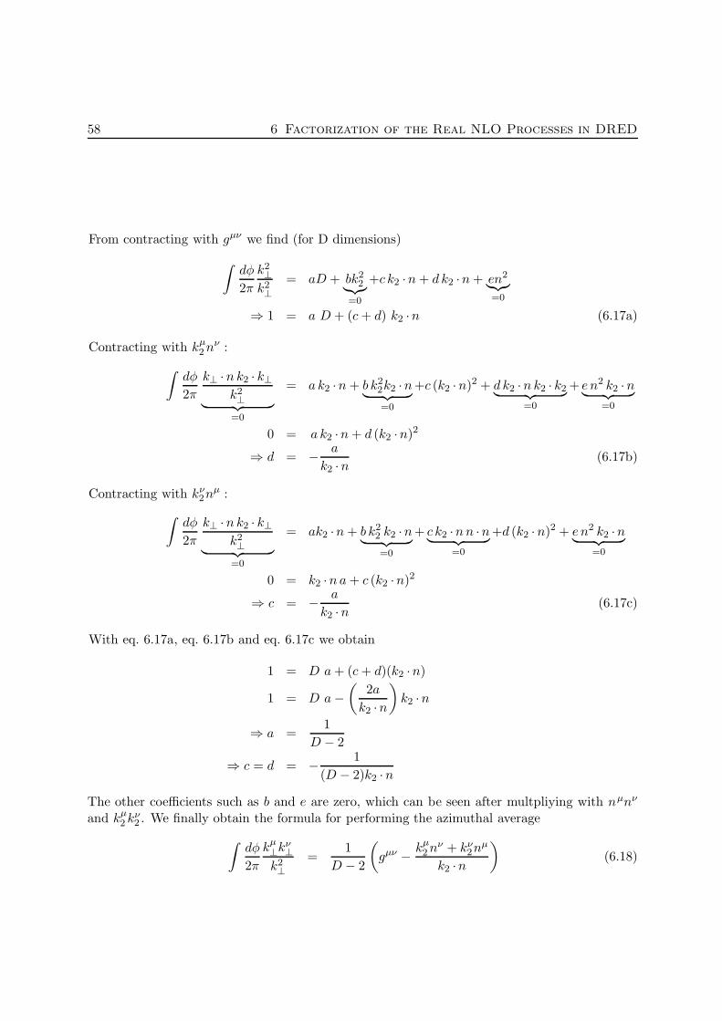
58 6 Factorization of the Real NLO Processes in DRED
From contracting with gµν we find (for D dimensions)
∫dφ
2π
k2⊥k2⊥
= aD + bk22︸︷︷︸
=0
+c k2 ·n+ d k2 ·n+ en2︸︷︷︸=0
⇒ 1 = a D + (c+ d) k2 ·n (6.17a)
Contracting with kµ2n
ν :
∫dφ
2π
k⊥ ·nk2 · k⊥k2⊥︸ ︷︷ ︸
=0
= a k2 ·n+ b k22k2 ·n︸ ︷︷ ︸=0
+c (k2 ·n)2 + d k2 ·nk2 · k2︸ ︷︷ ︸=0
+ e n2 k2 ·n︸ ︷︷ ︸=0
0 = a k2 ·n+ d (k2 ·n)2
⇒ d = − a
k2 ·n(6.17b)
Contracting with kν2n
µ :
∫dφ
2π
k⊥ ·nk2 · k⊥k2⊥︸ ︷︷ ︸
=0
= ak2 ·n+ b k22 k2 ·n︸ ︷︷ ︸=0
+ c k2 ·nn ·n︸ ︷︷ ︸=0
+d (k2 ·n)2 + e n2 k2 ·n︸ ︷︷ ︸=0
0 = k2 ·na+ c (k2 ·n)2
⇒ c = − a
k2 ·n(6.17c)
With eq. 6.17a, eq. 6.17b and eq. 6.17c we obtain
1 = D a+ (c+ d)(k2 ·n)
1 = D a−(
2a
k2 ·n
)k2 ·n
⇒ a =1
D − 2
⇒ c = d = − 1
(D − 2)k2 ·n
The other coefficients such as b and e are zero, which can be seen after multpliying with nµnν
and kµ2 k
ν2 . We finally obtain the formula for performing the azimuthal average
∫dφ
2π
kµ⊥k
ν⊥
k2⊥
=1
D − 2
(gµν − kµ
2nν + kν
2nµ
k2 ·n
)(6.18)
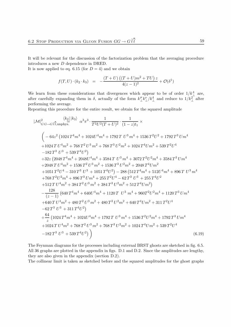
6.2 Stop Production via Gluon Fusion GG→ G t t 59
It will be relevant for the discussion of the factorization problem that the averaging procedureintroduces a new D dependence in DRED.It is now applied to eq. 6.15 (for D = 4) and we obtain
f(T,U) · (k2 · k3) = −(T + U)((T + U)m2 + TU
)z
4(z − 1)2+ O(δ1)
We learn from these considerations that divergences which appear to be of order 1/k4⊥ are,
after carefully expanding them in δ, actually of the form kµ⊥k
ν⊥/k
4⊥ and reduce to 1/k2
⊥ afterperforming the average.Repeating this procedure for the entire result, we obtain for the squared amplitude
|M|2G G→G et et,unphys.
〈k2| |k3〉= α3π3 · 1
T 2U2(T + U)2· 1
(1 − z)t1×
(− 64z2
(1024T 4m4 + 1024U 4m4 + 1792T U 3m4 + 1536T 2U2 + 1792T 3 Um4
+1024T U 4m2 + 768T 2 U3m2 + 768T 3 U2m2 + 1024T 4Um2 + 539T 2U4
−182T 3 U3 + 539T 4U2)
+32z(2048T 4m4 + 2048U 4m4 + 3584T U 3m4 + 3072T 2U2m4 + 3584T 3 Um4
+2048T U 4m2 + 1536T 2 U3m2 + 1536T 3 U2m2 + 2048T 4Um2
+1051T 2U4 − 310T 3 U3 + 1051T 4U2)− 288
(512T 4m4 + 512U4m4 + 896T U 3m4
+768T 2U2m4 + 896T 3 Um4 + 255T 2U4 − 62T 3 U3 + 255T 4U2
+512T U 4m2 + 384T 2 U3m2 + 384T 3 U2m2 + 512T 4Um2)
− 128
(z − 1)
(640T 4m4 + 640U4m4 + 1120T U 3 m4 + 960T 2U2m4 + 1120T 3 Um4
+640T U 4m2 + 480T 2 U3m2 + 480T 3 U2m2 + 640T 4Um2 + 311T 2U4
−62T 3 U3 + 311T 4U2)
+64
z
(1024T 4m4 + 1024U 4m4 + 1792T U 3m4 + 1536T 2U2m4 + 1792T 3 Um4
+1024T U 4m2 + 768T 2 U3m2 + 768T 3 U2m2 + 1024T 4Um2 + 539T 2U4
−182T 3 U3 + 539T 4U2))
(6.19)
The Feynman diagrams for the processes including external BRST ghosts are sketched in fig. 6.5.All 36 graphs are plotted in the appendix in figs. D.1 and D.2. Since the amplitudes are lengthy,they are also given in the appendix (section D.2).The collinear limit is taken as sketched before and the squared amplitudes for the ghost graphs
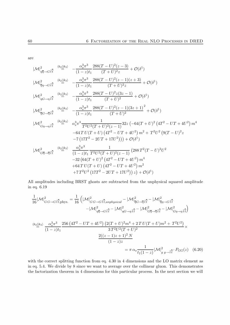
60 6 Factorization of the Real NLO Processes in DRED
are
|M|2ηη→G et et
〈k2||k3〉= − α3
sπ3
(1 − z)t1
288(T − U)2(z − 3)
(T + U)2z+ O(δ1)
|M|2ηη→G et et
〈k2||k3〉= − α3
sπ3
(1 − z)t1
288(T − U)2(z − 1)(z + 3)
(T + U)2z+ O(δ1)
|M|2ηG→η et et
〈k2||k3〉= − α3
sπ3
(1 − z)t1
288(T − U)2z(3z − 1)
(T + U)2+ O(δ1)
|M|2ηG→η et et
〈k2||k3〉= − α3
sπ3
(1 − z)t1
288(T − U)2(z − 1)(3z + 1)
(T + U)2
2
+ O(δ1)
|M|2Gη→η et et
〈k2||k3〉= α3
sπ3 1
T 2U2(T + U)2(z − 1)32z
(−64(T + U)2
(4T 2 − UT + 4U 2
)m4
−64T U(T + U)(4T 2 − UT + 4U 2
)m2 + T 2U2
(9(T − U)2z
−7(17T 2 − 2UT + 17U 2
)))+ O(δ1)
|M|2Gη→η et et
〈k2||k3〉=
α3sπ
3
(1 − z)t1
1
T 2U2(T + U)2(z − 1)
(288T 2(T − U)2U2
−32(64(T + U)2
(4T 2 − UT + 4U 2
)m4
+64T U(T + U)(4T 2 − UT + 4U 2
)m2
+7T 2U2(17T 2 − 2UT + 17U 2
))z)
+ O(δ1)
All amplitudes including BRST ghosts are subtracted from the unphysical squared amplitudein eq. 6.19
1
16|M|2
G G→G et et,phys.=
1
16
(|M|2
G G→G et et,unphysical− |M|2
ηG→η et et− |M|2
ηη→G et et
−|M|2ηη→G et et
− |M|2ηG→η et et
− |M|2Gη→η et et
− |M|2Gη→η et et
)
〈k2||k3〉=
α3sπ
3
(1 − z)t1
256(4T 2 − UT + 4U 2
) (2(T + U)2m4 + 2T U(T + U)m2 + T 2U2
)
3T 2U2(T + U)2×
2((z − 1)z + 1)2 N
(1 − z)z
= π αs1
t1(1 − z)|M|2
g g→et et·PGG(z) (6.20)
with the correct splitting function from eq. 4.30 in 4 dimensions and the LO matrix element asin eq. 5.4. We divide by 8 since we want to average over the collinear gluon. This demonstratesthe factorization theorem in 4 dimensions for this particular process. In the next section we will
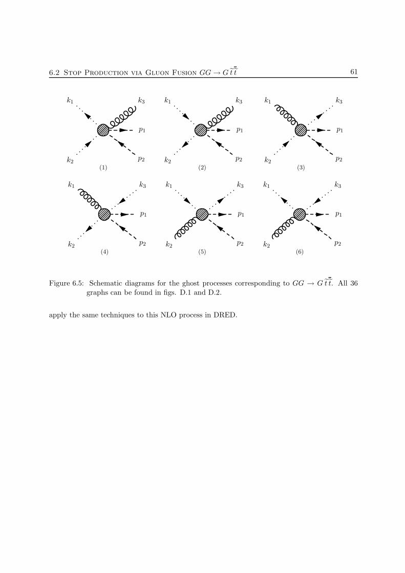
6.2 Stop Production via Gluon Fusion GG→ G t t 61
k2
k1
p2
p1
k3
(1)k2
k1
p2
p1
k3
(2)k2
k1
p2
p1
k3
(3)
k2
k1
p2
p1
k3
(4)k2
k1
p2
p1
k3
(5)k2
k1
p2
p1
k3
(6)
Figure 6.5: Schematic diagrams for the ghost processes corresponding to GG → G t t. All 36graphs can be found in figs. D.1 and D.2.
apply the same techniques to this NLO process in DRED.
62 6 Factorization of the Real NLO Processes in DRED
6.2.2 Mass Factorization in DRED
After introducing all the important tools in the last sections, we are now ready to perform thefactorization in DRED. There are two possibilities for the calculation of this amplitude, the oneintroduced in the last sections with the ε scalar and a second method where the vector fields arekept 4-dimensional. Both lead to the same result.As discussed in chapter 4 the factorization problem found by Beenakker et al. [1] for the processGG → Gt t shows up when processes are calculated with the second method. We illustratedin chapter 4 that this treatment leads to non-factorizable terms in the collinear limit. We alsofound that these terms vanish for m = 0 and are absent in DREG.
As discussed in chapter 4 we have two different partons, a gluon g and an ε scalar φ form-ing different partonic processes. Thus the following processes have to be considered
g g → g t t (6.21a)
g φ→ φ t t (6.21b)
φ g → φ t t (6.21c)
φφ→ g t t (6.21d)
After factorizing these processes separately we also need different splitting functions
g g → g (6.22a)
g φ→ φ (6.22b)
φ g → φ (6.22c)
φφ→ g (6.22d)
which we have already calculated in chapter 4.
Factorization of the D-dimensional Gluon Part (eq. 6.21a)
The Feynman diagrams for the gluonic processes are sketched in figs. 6.4 and D.3. Since theexpressions for the Feynman amplitudes are the same as in 4 dimensions, we refer to sectionD.2.For the Feynman diagrams including the BRST ghosts we refer to figs. 6.5, D.1 and D.2. Notethat there is no coupling of ε scalars and BRST ghosts.Since FormCalc calculates the polarization sum in 4 dimensions, we only use it to square theamplitudes and to calculate the color traces. The result then still includes the D-dimensionalpolarization vectors ε(k) which are calculated with the unphysical polarization sum in eq. A.7.This leads to a dimensional dependence of the squared amplitude. Due to the length, the resultis not given here.We parametrize the momenta k2 and k3 as in eq. 6.4 but with the index µ living in D dimensions.We substitute the scalar products of the momenta with the modified Mandelstam variables fromeq. 6.5 and use the relation in eq. 6.13 to eliminate S. This leads to terms depending on
6.2 Stop Production via Gluon Fusion GG→ G t t 63
1/(δ k⊥)2, 1/(δk⊥)4, T, U and D. Now the collinear limit is taken by expanding these terms inδ around 0 to the zeroth order
|M|2g g→g et et
〈k2||k3〉= − α3
sπ3
(1 − z)t1
32
T 2U2(T + U)2(z − 1)zk2⊥×
(256(2D − 3)m2U2
(4T 2 − UT + 4U 2
)(k1 · k⊥)2z2
+ 256(2D − 3)m2(T + U)2(4T 2 − UT + 4U 2
)(k4 · k⊥)2z2
− 512(2D − 3)m2U(T + U)(4T 2 − UT + 4U 2
)(k1 · k⊥)(k4 · k⊥)z2
+(512(T + U)2
(4T 2 − UT + 4U 2
)(z − 1)2
(z2 + 1
)m4
+ 512TU(T + U)(4T 2 − UT + 4U 2
)(z − 1)2
(z2 + 1
)m2
+ T 2U2((
512D((z − 1)z + 1)2 + z(z((1967 − 970z)z − 2798) + 1967) − 970)T 2
− 2U(64D((z − 1)z + 1)2 + z(z((175 − 74z)z − 334) + 175) − 74
)T
+U2(512D((z − 1)z + 1)2 + z(z((1967 − 970z)z − 2798) + 1967) − 970 )
))k2⊥
)+ O(δ1)
There are still terms depending on kµ⊥/k
2⊥ and (kµ
⊥kν⊥)/k2
⊥. The former terms do not contributedue to the vanishing phase space integral deduced in eq. 6.14. The latter terms are averagedazimuthally with eq. 6.18 (this is where another dimensional dependence of 1/(D−2) enters thecalculation). The result simplifies to
|M|2g g→g et et,unphys.
〈k2||k3〉= − α3
sπ3
(1 − z)t1
32
(D − 2)T 2U2(T + U)2(z − 1)z×
(256(T + U)2
(4T 2 − UT + 4U 2
) (2D((z − 1)z + 1)2 + z(z(−4(z − 2)z − 11) + 8) − 4
)m4
+ 256TU(T + U)(4T 2 − UT + 4U 2
) (2D((z − 1)z + 1)2 + z(z(−4(z − 2)z − 11) + 8) − 4
)m2
+ (D − 2)T 2U2((
512D((z − 1)z + 1)2 + z(z((1967 − 970z)z − 2798) + 1967) − 970)T 2
− 2U(64D((z − 1)z + 1)2 + z(z((175 − 74z)z − 334) + 175) − 74
)T
+U2(512D((z − 1)z + 1)2 + z(z((1967 − 970z)z − 2798) + 1967) − 970
)) )(6.23)
There are six different ghost processes (fig. 6.5) each having 6 different topologies (figs. D.1 andD.2)
ηη → g t t; ηη → g t t; gη → η t t;
g η → η t t; gη → η t t; gη → η t t;(6.24)
These amplitudes are identical to the ones given in section D.2 but with the momenta living inD dimensions. Then the collinear limit can be taken analogous to the last process, and after
64 6 Factorization of the Real NLO Processes in DRED
expanding in δ around 0 we obtain
|M|2ηη→g et et
〈k2||k3〉= − α3
sπ3
(1 − z)t1
288(T − U)2(z − 1)(z + 3)
(T + U)2z+ O(δ1)
|M|2ηη→g et et
〈k2||k3〉= − α3
sπ3
(1 − z)t1
288(T − U)2(z − 3)
(T + U)2z+ O(δ1)
|M|2gη→η et et
〈k2||k3〉= − α3
sπ3
(1 − z)t1
288(T − U)2z(3z − 1)
(T + U)2+ O(δ1)
|M|2gη→η et et
〈k2||k3〉= − α3
sπ3
(1 − z)t1
288(T − U)2(1 − z)(3z + 1)
(T + U)2+ O(δ1)
|M|2gη→η et et
〈k2||k3〉= − α3
sπ3
(1 − z)t1
32z
(D − 2)T 2U2(T + U)2(z − 1)×
(−128(T + U)2
(4T 2 − UT + 4U 2
)m4
−128TU(T + U)(4T 2 − UT + 4U 2
)m2
+(D − 2)T 2U2(9(T − U)2z −7
(17T 2 − 2UT + 17U 2
)) )+ O(δ1)
|M|2g η→eη et et
〈k2||k3〉= − α3
sπ3
(1 − z)t1
1
(D − 2)T 2U2(T + U)2(z − 1)
(288(D − 2)T 2(T − U)2U2
−32(128(T + U)2
(4T 2 − UT + 4U 2
)m4
+128TU(T + U)(4T 2 − UT + 4U 2
)m2
+7(D − 2)T 2U2(17T 2 − 2UT + 17U 2
))z)
+ O(δ1)
Subtracting the ghost processes as the unphysical polarization states from the D-dimensionalgluon process, we find (neglecting higher orders δ)
1
8|M|2
gg→g et et
〈k2||k3〉=
〈k2||k3〉=
α3sπ
3
t1(1 − z)· N · 2((1 − z)z + 1)2
(z − 1)z×
256(4T 2 − UT + 4U 2
) (4(T + U)2m4 + 4TU(T + U)m2 + (D − 2)T 2U2
)
3T 2U2(T + U)2
= αsπ1
t1(1 − z)|M|2
gg→et et·Pgg(z) (6.25)
This is equal to the result in DRED. Obviously, this process factorizes as expected. This resultis also part of the non-factorizable result in eq. 4.2. The squared amplitude |M|2
g g→et etwas
calculated in section 5.2 (eq. 5.3). The gluon-gluon splitting function is the one given in eq. 4.30
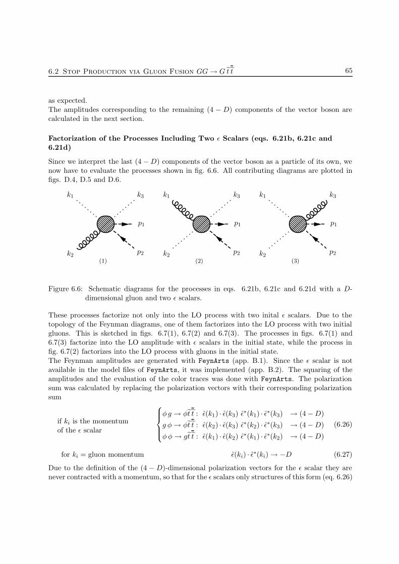
6.2 Stop Production via Gluon Fusion GG→ G t t 65
as expected.The amplitudes corresponding to the remaining (4 − D) components of the vector boson arecalculated in the next section.
Factorization of the Processes Including Two ε Scalars (eqs. 6.21b, 6.21c and6.21d)
Since we interpret the last (4 −D) components of the vector boson as a particle of its own, wenow have to evaluate the processes shown in fig. 6.6. All contributing diagrams are plotted infigs. D.4, D.5 and D.6.
k2
k1
p2
p1
k3
(1)k2
k1
p2
p1
k3
(2)k2
k1
p2
p1
k3
(3)
Figure 6.6: Schematic diagrams for the processes in eqs. 6.21b, 6.21c and 6.21d with a D-dimensional gluon and two ε scalars.
These processes factorize not only into the LO process with two inital ε scalars. Due to thetopology of the Feynman diagrams, one of them factorizes into the LO process with two initialgluons. This is sketched in figs. 6.7(1), 6.7(2) and 6.7(3). The processes in figs. 6.7(1) and6.7(3) factorize into the LO amplitude with ε scalars in the initial state, while the process infig. 6.7(2) factorizes into the LO process with gluons in the initial state.
The Feynman amplitudes are generated with FeynArts (app. B.1). Since the ε scalar is notavailable in the model files of FeynArts, it was implemented (app. B.2). The squaring of theamplitudes and the evaluation of the color traces was done with FeynArts. The polarizationsum was calculated by replacing the polarization vectors with their corresponding polarizationsum
if ki is the momentumof the ε scalar
φ g → φt t : ε(k1) · ε(k3) ε∗(k1) · ε∗(k3) → (4 −D)
g φ→ φt t : ε(k2) · ε(k3) ε∗(k2) · ε∗(k3) → (4 −D)
φφ→ gt t : ε(k1) · ε(k2) ε∗(k1) · ε∗(k2) → (4 −D)
(6.26)
for ki = gluon momentum ε(ki) · ε∗(ki) → −D (6.27)
Due to the definition of the (4 −D)-dimensional polarization vectors for the ε scalar they arenever contracted with a momentum, so that for the ε scalars only structures of this form (eq. 6.26)

66 6 Factorization of the Real NLO Processes in DRED
k2
k1
p2
p1
k3
〈k2||k3〉−→
k2
k1
p2
p1
(1) Schematic diagrams for the process φg → φet et with a D-dimensional gluon and ε scalars. Thisprocess factorizes into the 2 → 2 process with ε scalars in the initial state.
k2
k1
p2
p1
k3
〈k2||k3〉−→
k2
k1
p2
p1
(2) Schematic diagrams for the process gφ → φet et with a D-dimensional gluon and ε scalars. Incontrast to the other two processes involving ε scalars, this process factorizes into the 2 → 2 processwith gluons in the initial state.
k2
k1
p2
p1
k3
〈k2||k3〉−→
k2
k1
p2
p1
(3) Schematic diagrams for the process φφ → get et with a D-dimensional gluon and ε scalars. Thisprocess factorizes into the 2 → 2 process with ε scalars in the initial state.
Figure 6.7: All schematic NLO diagrams with their corresponding LO processes.
6.2 Stop Production via Gluon Fusion GG→ G t t 67
appear. However, the polarization vectors of the gluons can also be contracted to momenta, e.g.
ε(ki)µkµ ε
∗(kj)νpν → −k · p
The squared amplitudes after performing the polarization sums and color traces are lengthy.They are shown in section D.3 where they are expressed in terms of the kinematic variables for5 legs defined in eq. A.4. Using eq. 6.4 and eq. 6.13 we take the collinear limit and substitute S.After expanding the terms in δ around 0 to zeroth order we calculate the squared amplitudesfor the process in fig. 6.6(1) (eq. 6.21c)
1
8
4 −D
D − 2|M |2
φ g→φet et
〈k2||k3〉=
=1
8
1
t1(1 − z)· 2z(1 − z)
4 −D
D − 2N ·α3
sπ3 · 2048
(4T 2 − UT + 4U 2
)(D − 4)
3(T + U)2+ O(δ1)
= α3sπ
3 · 1
t1(1 − z)
256(4T 2 − UT + 4U 2
)(4 −D)
3(T + U)2· 2z(1 − z)
4 −D
D − 2N
=1
t1(1 − z)αsπ Pφg(z) |M|2
φφ→et et(6.28)
with the splitting function Pφg(z) from eq. 4.32 for a gluon splitting into two ε scalars.For the process where the emitted particle is an ε scalar (fig. 6.6(2), eq. 6.21b) we find
1
8
D − 2
4 −D|M |2
gφ→φet et
〈k2||k3〉=
= (D − 2)α3
sπ3
(1 − z)t1
Nz
(z − 1)×
512(4T 2 − UT + 4U 2
) (T 2k2
⊥U2 + 4(m2Uk1 · k⊥ −m2(T + U)k4 · k⊥)2
)
3T 2U2(T + U)2k2⊥
+ O(δ1)
1
=αsπ
(1 − z)t1· 2Nz
(1 − z)×
256α2sπ
2(4T 2 − UT + 4U 2
) (4(T + U)2m4 + 4TU(T + U)m2 + (D − 2)T 2U2
)
3T 2U2(T + U)2
68 6 Factorization of the Real NLO Processes in DRED
=1
t1(1 − z)αsπ P (z)φφ |M|2
gg→et et(6.29)
with the splitting function eq. 4.34, P (z)φφ, where an ε scalar radiates another ε scalar anda gluon enters the factorized matrix element. This is the process which factorizes to the LOprocess with gluons in the initial state.The process with two initial ε scalars and a final gluon (fig. 6.6(3), eq. 6.21d) factorizes
1
8
4 −D
4 −D|M |2
φφ→get et
〈k2||k3〉=
=1
(1 − z)t1π3α3
s
256(4 −D)(4T 2 − UT + 4U 2
)
3(T + U)2· 2N (1 − z)
z+ O(δ1)
= α3sπ
3 1
t1(1 − z)
2(1 − z)N
z
256(4 −D)(4T 2 − UT + 4U 2
)
3(T + U)2
=1
t1(1 − z)αsπ P (z)gφ|M|2
φ φ→et et(6.30)
with the splitting function in eq. 4.33 where the gluon is the collinearly radiated particle.Each process has to be multiplied with a factor of D−2 (4−D) for the gluon (ε scalar) enteringthe LO process and for every gluon (ε scalar) entering the NLO process we have to divide by afactor of D − 2 (4 −D).The LO results can be found in section 5.2 and the corresponding splitting functions in section4.4.
These results demonstrate that all four partonic processes factorize in the desired way into theproduct of a splitting function, the LO process and the collinear pole, and therefore are inaccordance with the mass factorization theorem.The seemingly non-factorizable result (eq. 4.2) can be recovered by adding all the individualcontributions in eqs. 6.25, 6.28, 6.29 and 6.30.
1The terms have to be azimuthally averaged, since the intermediate result still depends on k⊥.

7 Discussion
If DRED is realized by introducing an additional (4 − D)-component parton, new processesincluding external ε scalars arise which have to be evaluated individually. Following this ideathe results from chapter 6 demonstrate that these individual processes factorize into a productof the LO process, a splitting function and the pole as desired. All problematic terms in eq. 4.2are interpreted as partonic processes with their corresponding splitting functions.In this section we summarize the procedure of separating the squared amplitude into processesconsidering dimensionally reduced gluons and their remaining (4−D) components. Furthermorewe motivate the individual factorization of processes in terms of the new partons, which, seenas one single physical process involving 4-dimensional gluons, fail to factorize.We investigate why the factorization problem is absent in the massless limit and discuss, whyin contrast to the second process described in this work, the first process factorizes without theneed for ε scalars.
7.1 Interpretation of the Squared Amplitudes in DRED
In chapter 4 we tried to factorize the real NLO processes by expressing them as
1
8|M|2
GG→Get et
〈k2||k3〉= 1
t1(1−z)αsπ · |M|2GG→et et
after taking the collinear limit. However, we find non-factorizable terms (eq. 4.2).As the first step to gain insight into the origin of this problem we split the squared amplitudewith 4-component gluons into processes including D-dimensional gluons (g) and ε scalars (φ).The squared amplitude with initial 4-dimensional gluons can be split
|M|2GG→Get et
= |M|2gg→get et
+ |M|2g φ→φet et
+ |M|2φ g→φet et
+ |M|2φφ→get et
=∑
i,j=g,φ
(|M|2
g i→jet et+ |M|2
φ i→jet et
)(7.1)
Interference terms including an ε scalar and a gluon vanish:
∑
s
εsµε∗sν MµM∗ν =
∑
s
εsρε∗sσ MρM∗σ + εsi ε
∗sj MiM∗j + (εsρε
∗sj MρM∗j + εsi ε
∗sσ MiM∗σ)
70 7 Discussion
and the interference term in the parentheses are zero because
∑
s
εsρε∗sj = −gρj = 0
In the collinear limit we find
|M|2GG→Get et
=∑
i,j,k=g,φ
|M|2i j→k et et
〈k2||k3〉=
αsπ
t1(1 − z)
∑
i=g,φ
Pg i(z)|M|2gg→et et
+∑
i=g,φ
Pφ i(z)|M|2φφ→et et
(7.2)
As we saw from the derivations in chapter 5, the squared amplitudes for |M|2gg→et et
and |M|2φφ→et et
are not proportional to one another. This indicates that factorization only works in the sensethat these subprocesses (eq. 7.2) factorize separately, which motivates us to consider g and φ asseparate partons.In DREG all contributions with external ε scalars are absent and therefore factorization obviouslyfollows from eq. 7.2 as well.
7.2 Mass Dependence of the Factorization Problem
For massless squarks we found that the NLO process factorizes without problems into the correctLO process without treating the ε scalars as separate particles
1
8|M|2
GG→Get et
〈k2||k3〉=
m=0
αsπ
t1(1 − z)·(
256α2sπ
2(4T 2 − UT + 4U 2
)
3(T + U)2· 2((z − 1)z + 1)2
(1 − z)zN
)
For m → 0 all terms violating the factorization theorem in eq. 4.2 vanish and it factorizes asdesired. This was also noted for other processes in [1], [2] and [30].The absence of the factorization problem can be reconstructed from the LO results for initial εscalars and initial gluons. The LO process with initial ε scalars is
|M|2φφ→et et
= α2sπ
2 256(4 −D)(4T 2 − UT + 4U 2
)
3(T + U)2(7.3)
in difference to the gluon LO result which exhibits a more complicated structure
|M|2gg→et et
= α2sπ
2 512(4T 2 − UT + 4U 2
) (4(T + U)2m4 + 4TU(T + U)m2 + (D − 2)T 2U2
)
3T 2U2(T + U)2
m=0= α2
sπ2 256(D − 2)
(4T 2 − UT + 4U 2
)
3(T + U)2(7.4)

7.2 Mass Dependence of the Factorization Problem 71
For the massless limit, both LO processes yield the same expression. Now we are able to pullthe squared amplitude out of the sum in eq. 7.2, and only sums of the splitting functions remain:
1
8|M|2
GG→et et
〈k2||k3〉=
m=0α3
sπ3 256(D − 2)
(4T 2 − UT + 4U 2
)
3(T + U)2·(
2N(D − 4)z
(D − 2)(z − 1)
+2N(D − 4)(z − 1)
(D − 2)z+ 2N(D − 4)
(z − 1)
(D − 2)z +
2N((z − 1)z + 1)2
(1 − z)z
)
= α3sπ
3 256(D − 2)(4T 2 − UT + 4U 2
)
3(T + U)2
((Pφφ + Pφg)
(4 −D)
(D − 2)+ Pφ g + Pgg
)
= α3sπ
3 512(4T 2 − UT + 4U 2
)
3(T + U)2
(2N((z − 1)z + 1)2
(1 − z)z
)(7.5)
Even without taking the limit D → 4, the last line represents the correct result for the splittingfunction PGG(z). This shows that the splitting functions eqs. 4.30, 4.32, 4.33 and 4.34 sum upto give twice the pure gluon splitting function eq. 4.30.
In [2] the reason for this behaviour in the massless limit (which is similar for the process GG→ ttinvestigated in [2]) is suspected to be connected with the occurence of the double pole. In theiranalysis, the massless and the massive cases are distinguished by the appearance of the doublepole 1/t21 which has to be azimuthally averaged. In the process at hand, we also find terms withdouble poles 1/t21 and cope with them in chapter 6.A closer look at the NLO squared amplitude in the collinear limit before averaging (e.g. ineq. 6.29, the important part is again given in eq. 7.6) shows that in the massless limit the termsproportional to kµ
⊥ kν⊥/k
2⊥ vanish
|M|2 ∝(4T 2 − UT + 4U 2
) (T 2k2
⊥U2 + 4(m2Uk1 · k⊥ −m2(T + U)k4 · k⊥)2
)
3T 2U2(T + U)2k2⊥
m=0=
(4T 2 − UT + 4U 2
)
3(T + U)2(7.6)
This implies that the azimuthal average over k⊥ is trivial in this case. Since we have to averageover k⊥ for the massive case in both DRED and DREG, the appearance of the double poles hasno particular connection to the appearance of the ε scalars and to the absence of the factoriza-tion problem.As shown in 7.6 for m = 0 all terms including kµ
⊥kν⊥/k
2⊥ which would need to be averaged are
zero.In this process, the LO squared amplitudes with ε scalars do not introduce a new mass depen-dence. Furthermore the parts in eq. 7.3 and eq. 7.4 containing a prefactor of (4−D) and D areequal for both amplitudes including gluons and ε scalars.The terms in eq. 7.6 which do not have a dimensional factor are instead proportional to m2. Itwould be interesting to understand if these mass factors are always connected to the absence of

72 7 Discussion
a dimensional dependence as this would explain the absence of the factorization problem in themassless limit.
7.3 Appearance of the Factorization Problem in Specific
Processes
For further calculations it would be useful to see for which kinds of processes in DRED the factor-ization problems appears, thus requiring us to calculate with ε scalars. From the calculations inthis work, we can at least infer necessary conditions for the need of ε scalars in specific processes.
No Need for ε Scalars: qq → Gt t and qq → Gt t
As we saw in chapter 6, the process qq → Gt t factorizes with or without treating the (4 −D)component of the gluon as a separate particle.
The LO process qq → t t is the same for both DRED and DREG since obviously no correspondingLO process with external ε scalars can be formed. This implies that the real NLO correctionto this process can only factorize into this specific squared amplitude in the collinear limit, butwith different splitting functions for the ε scalar-quark (eq. 4.29) and a gluon-quark splitting(eq. 4.27). As we see, both splitting functions add up to give the 4-dimensional quark-gluonsplitting function:
Pφq(z) + Pgq(z) = C2(r)
(1
2(4 −D)z +
z((D − 2)z − 4) + 4
z
)
= C2(r)1 + (1 − z)2
z(7.7)
= PGφ(z)
This is obvious from the definition of the ε scalar.Since there is only one LO result the absence of the factorization problem is clear with eq. 7.2.
Now we will briefly investigate another process where the factorization problem is also absent:qq → gt t. The LO Feynman diagrams are shown in fig. 7.1. Here we see, that two distinct LOprocesses are present, one with a gluon and one with an ε scalar in the S channel . So, in thecollinear limit, all real NLO corrections yield one of the two processes (fig. 7.1(1) or fig. 7.1(2)).But since their kinematical structure is the same and the splitting functions add up as in eq. 7.7,the result factorizes as desired.

7.3 Appearance of the Factorization Problem in Specific Processes 73
q
tq
gt
(1)
q
tq
φt
(2)
Figure 7.1: Feynman diagrams for qq → tt.
Need for ε Scalars: gg → gt t and gg → gt t
In the process
GG→ t t
the amplitudes are of a more complicated structure. Here we have two different LO processes,one with external gluons and one with external ε scalars. As we have discussed before, thesesquared LO amplitudes differ in their kinematical structure due to the three gluon coupling andthe gluon-two ε coupling. This and the fact that there is no two-squark ε scalar coupling implythese differences.If we now calculate the real NLO corrections for both gluons and ε scalars, we see that thedifferent initial NLO states lead to different LO processes:
gg → gt tfactorizes−→ gg → t t (7.8a)
gφ→ φt tfactorizes−→ gg → t t (7.8b)
φφ→ gt tfactorizes−→ φφ→ t t (7.8c)
φg → φt tfactorizes−→ φφ→ t t (7.8d)
Since the LO squared amplitudes for eq. 7.8a and eq. 7.8c differ in the kinematic structure, thesum does not factorize but the processes have to be treated separately as in eq. 7.2.The process investigated in [1] and [2] (in fig. 7.2) shows a similar behaviour. The NLO processescan be classified by the LO processes they factorize into, which are
gg → t t (7.9a)
φ g → t t (7.9b)
gφ→ t t (7.9c)
φφ→ t t (7.9d)
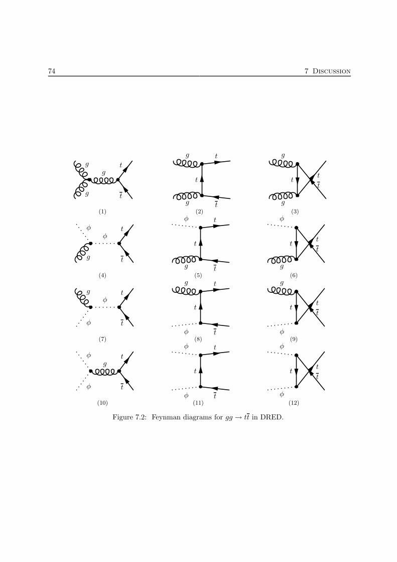
74 7 Discussion
g
tg
gt
(1)
g
t
t
g
t
(2)
g
tt
g
t
(3)
φ
tg
φt
(4)
φ
t
t
g
t
(5)
tt
φ
g
t
(6)
g
tφ
φt
(7)φ
g
t
t
t
(8)φ
g
tt
t
(9)
φ
tφ
gt
(10)
φ
t
t
φ
t
(11)
φ
tt
φ
t
(12)
Figure 7.2: Feynman diagrams for gg → tt in DRED.

7.3 Appearance of the Factorization Problem in Specific Processes 75
Each is represented by one row in fig. 7.2. Each column would sum up to give the correspond-ing diagram for a 4 component gluon but this is spoiled since after factorization the individualdiagrams come with different splitting functions.On the other hand, since the squared LO processes differ in their kinematical structure it is not
possible to pull them out of the sum in eq. 7.2 as in the case qq → t t.
Different Squared Amplitudes for Processes Involving the ε Scalar and the Gluon
From the previous discussion one can conjecture that at tree level the appearance of the factor-ization problem is connected to external ε scalars in LO cross sections. In section 4.3 we founddifferences in the kinematic structure of some vertices originating from the same 4 componentgluon coupling, summarized here:
• the V V V vertex in comparison with the φφV vertex
• the V V V V vertex in comparison with the φφV V and the φφφφ vertex
• absence of the φF F vertex
• absence of the φφφ, φV V , φφφV and φV V V vertices
The other vertices including ε scalars differ only in the dimension of the Lorentz indices.So we conjecture that if external gluons appear in the LO process and thus one or more ofthe “critical” vertices are included, the squared LO amplitudes for the D-dimensional gluondiffer from those including its (4 −D) component, and that this gives rise to the factorizationproblem.
8 Conclusion
Almost 20 years ago, Beenakker et al. [1] found non-factorizable terms in a QCD process whichwas calculated in DRED, rendering this regularization scheme questionable. The problem hadnot shown up when the calculation was done in DREG. In [1], [2] and [30] it was found that thisfactorization problem vanishes in the massless limit.Recently, Signer and Stockinger interpreted the vector and scalar components of the gluon inDRED as separate partons, a D component gluon and the ε scalar [2]. The non-factorizableterms then turned out to be products of splitting functions and partonic LO processes involvingε scalars.It was the aim of this work to investigate the method proposed in [2] by applying it to the SUSY
QCD processes qq → G t t and GG → G t t. Following this idea it is shown in this work thatthis method can also be applied to solve the factorization problem for the processes mentionedabove. The detailed approach to mass factorization in massive SUSY QCD is demonstrated andthe splitting functions and Feynman rules for the ε scalar are derived.
We have found that for the process
qq → G t t (8.1)
the factorization problem does not appear, and we explain this with the fact that no ε scalarsappear in the LO process. This implies that even though ε scalars appear in the NLO process,they disappear in the collinear limit and the result factorizes like in 4 dimensions.For the second process investigated in this work,
GG→ G t t (8.2)
we find non-factorizable terms analogous to [1] and [2]. After treating the scalar as a parton ofits own, all individual NLO results factorize as desired into products of the LO processes andtheir corresponding splitting functions. All unusual terms encountered before can be interpretedin this manner.
The factorization is demonstrated by setting the radiated particle collinear to one of the initialparticles. For the process in eq. 8.2 we found double poles of the form 1/t21. An importantingredient to cope with these singularities is the integration over the unobservable azimuthalangle of the collinear particle, e.g. the gluon.In the massless case of eq. 8.2, these double singularities vanish before being azimuthally aver-aged.

77
An essential factor for the appearance of the factorization problem is the presence of externalvector particles involving vertices which change their kinematic structure after being rewrittenwith an ε scalar. If they appear we find differences in the kinematic structure of individualresults (including ε scalars and gluons) belonging to the same physical process in DRED whichgive rise to the factorization problem.These differences in the squared amplitudes are also decisive for the absence of the factorizationproblem in the massless limit. In this context, we also observe that there is a connection betweenthe appearance of mass terms and the dimensional dependence which seems essential for thisbehaviour, namely that terms which do not have a dimensional dependence carry a mass factor.It would be desirable to explore this phenomenon further and to investigate the consistency ofDRED in a precise analysis of the factorization in real NNLO.

A Conventions and Notations
A.1 Conventions and Notations
General Definitions
In this work we use the metric tensor
gµν = diag(1,−1,−1,−1)
where the gµν denotes the metric tensor in 4 dimensions.The scalar product of two vectors is denoted with
k · p = kµ pµ
unless otherwise noted, the indices are in 4 dimensions.The dimension of the Lorentz indices is indicated by the letters used, with greek indices for4 or D dimensions (µ, ν, ρ . . .) and with latin indices for 4 − D dimensions (i, j, k . . .). Thecorresponding objects (such as polarization vectors, metric tensor, Dirac matrices) are tilded x(D dim.) or hatted x (4 −D dim.).The trace of the metric tensor in arbitrary dimensions is defined as
gµµ = 4 gρ
ρ = D gii = 4 −D (A.1)
Mandelstam Variables
k2
k1
p2
p1
(1)k2
k1
k3
p2
p1
(2)
Figure A.1: Sketched processes with denotation for the momenta.
The kinetic variables are needed for 4 and for 5 external legs in this work. The notation isdisplayed in fig. A.1.Since in this work only massive final state particles appear in 2 → 2 processes, the Mandelstam
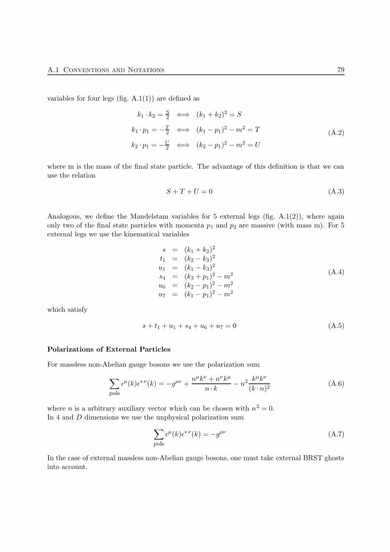
A.1 Conventions and Notations 79
variables for four legs (fig. A.1(1)) are defined as
k1 · k2 = S2 ⇐⇒ (k1 + k2)
2 = S
k1 · p1 = −T2 ⇐⇒ (k1 − p1)
2 −m2 = T
k2 · p1 = −U2 ⇐⇒ (k2 − p1)
2 −m2 = U
(A.2)
where m is the mass of the final state particle. The advantage of this definition is that we canuse the relation
S + T + U = 0 (A.3)
Analogous, we define the Mandelstam variables for 5 external legs (fig. A.1(2)), where againonly two of the final state particles with momenta p1 and p2 are massive (with mass m). For 5external legs we use the kinematical variables
s = (k1 + k2)2
t1 = (k2 − k3)2
u1 = (k1 − k3)2
s4 = (k3 + p1)2 −m2
u6 = (k2 − p1)2 −m2
u7 = (k1 − p1)2 −m2
(A.4)
which satisfy
s+ t1 + u1 + s4 + u6 + u7 = 0 (A.5)
Polarizations of External Particles
For massless non-Abelian gauge bosons we use the polarization sum
∑
pols
εµ(k)ε∗ ν(k) = −gµν +nµkν + nνkµ
n · k − n2 kµkν
(k ·n)2(A.6)
where n is a arbitrary auxiliary vector which can be chosen with n2 = 0.In 4 and D dimensions we use the unphysical polarization sum
∑
pols
εµ(k)ε∗ ν(k) = −gµν (A.7)
In the case of external massless non-Abelian gauge bosons, one must take external BRST ghostsinto account.

80 A Conventions and Notations
The polarization sum for ε scalars is
∑
pols
εµ(k)εν(k) = −gµν (A.8)
where the metric tensor is in (4 −D) dimensions.
The polarization vectors are defined in such a way that they obey
∑
pols
ε∗(p)µ ε∗µ(k) ε(p)ν ε
ν(k) = gµνgµν = 4 (A.9)
∑
pols
ε∗(p)µ ε∗µ(k) ε(p)ν ε
ν(k) = gµν gµν = 4 −D (A.10)
∑
pols
ε∗(p)µ ε∗(k)µ ε(p)ν ε
ν(k) = gµν gµν = D (A.11)
and further (only for physical polarizations)
ε(p) · p = 0 ε(p) · p = 0 ε(p) · p = 0 (A.12)
The polarization sum for fermions is
∑
s
us(k)us(k) = /k +m
∑
s
vs(k)vs(k) = /k −m(A.13)
where u denotes the incoming particle, u the outgoing particle, v the outgoing antiparticle andv the incoming antiparticle.
Numerator Algebra
For the evaluation of Dirac matrices we refer to [28] and generalize the results for D- and(4 −D)-dimensional indices
D dimensions : Tr [γµγν ] = 4gµν
4 −D dimensions : Tr[γiγj
]= 4gµν (A.14)
mixed dimensions : Tr[γµγi
]= 0
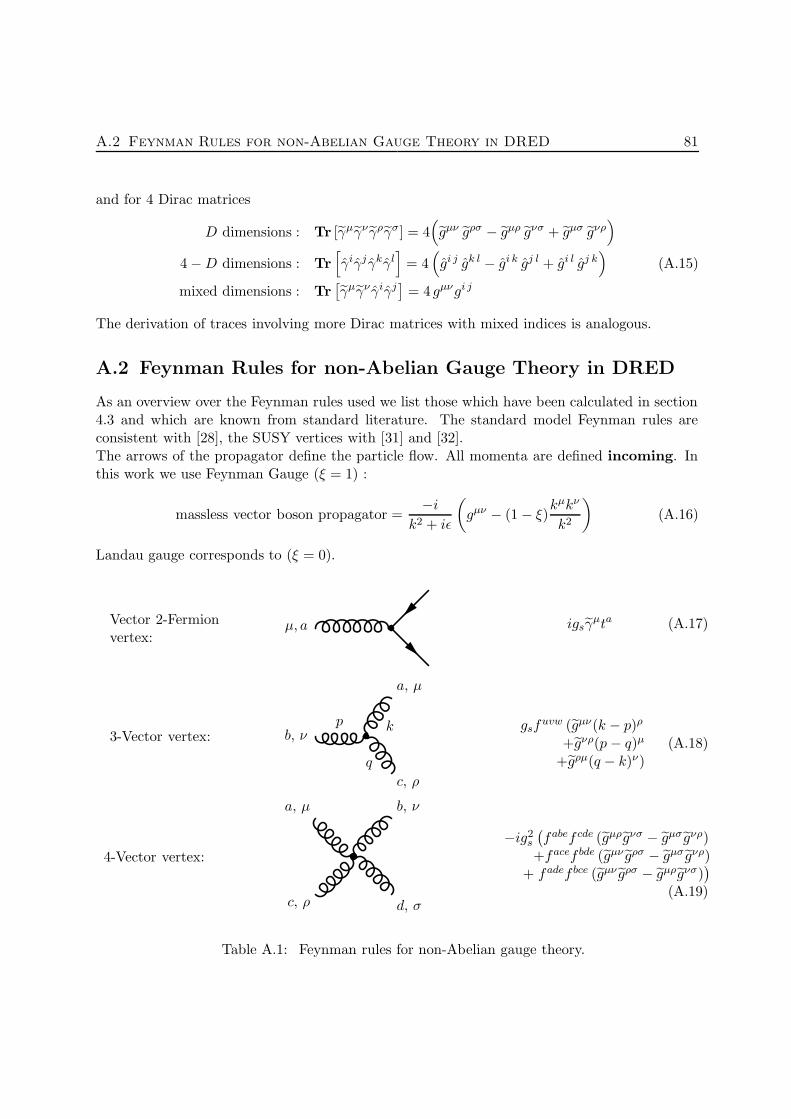
A.2 Feynman Rules for non-Abelian Gauge Theory in DRED 81
and for 4 Dirac matrices
D dimensions : Tr [γµγν γργσ] = 4(gµν gρσ − gµρ gνσ + gµσ gνρ
)
4 −D dimensions : Tr[γiγj γkγl
]= 4
(gi j gk l − gi k gj l + gi l gj k
)(A.15)
mixed dimensions : Tr[γµγν γiγj
]= 4 gµνgi j
The derivation of traces involving more Dirac matrices with mixed indices is analogous.
A.2 Feynman Rules for non-Abelian Gauge Theory in DRED
As an overview over the Feynman rules used we list those which have been calculated in section4.3 and which are known from standard literature. The standard model Feynman rules areconsistent with [28], the SUSY vertices with [31] and [32].The arrows of the propagator define the particle flow. All momenta are defined incoming. Inthis work we use Feynman Gauge (ξ = 1) :
massless vector boson propagator =−i
k2 + iε
(gµν − (1 − ξ)
kµkν
k2
)(A.16)
Landau gauge corresponds to (ξ = 0).
Vector 2-Fermionvertex:
µ, a igsγµta (A.17)
3-Vector vertex:p
q
kb, ν
c, ρ
a, µ
gsfuvw (gµν(k − p)ρ
+gνρ(p− q)µ
+gρµ(q − k)ν)(A.18)
4-Vector vertex:
c, ρ
a, µ
d, σ
b, ν
−ig2s
(fabef cde (gµρgνσ − gµσ gνρ)
+facef bde (gµν gρσ − gµσ gνρ)+ fadef bce (gµν gρσ − gµρgνσ)
)
(A.19)
Table A.1: Feynman rules for non-Abelian gauge theory.
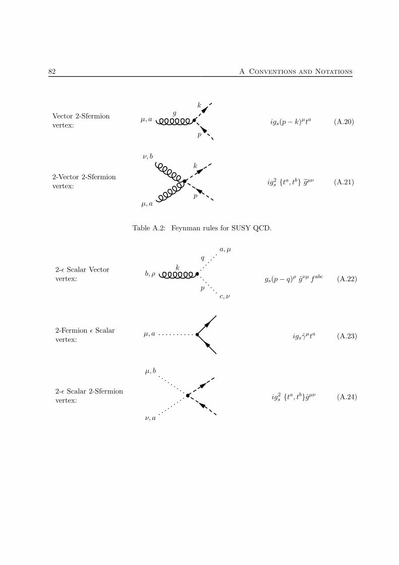
82 A Conventions and Notations
Vector 2-Sfermionvertex:
g
p
k
µ, a igs(p− k)µta (A.20)
2-Vector 2-Sfermionvertex:
p
k
µ, a
ν, b
ig2s {ta, tb} gµν (A.21)
Table A.2: Feynman rules for SUSY QCD.
2-ε Scalar Vectorvertex:
k
p
q
b, ρ
c, ν
a, µ
gs(p− q)ρ gνµ fabc (A.22)
2-Fermion ε Scalarvertex:
µ, a igsγµta (A.23)
2-ε Scalar 2-Sfermionvertex:
ν, a
µ, b
ig2s {ta, tb}gµν (A.24)
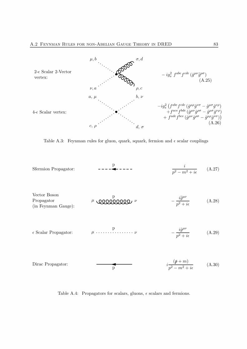
A.2 Feynman Rules for non-Abelian Gauge Theory in DRED 83
2-ε Scalar 2-Vectorvertex:
ν, a
µ, b
ρ, c
σ, d
− ig2s f
abef cde (gµν gρσ)(A.25)
4-ε Scalar vertex:
c, ρ
a, µ
d, σ
b, ν
−ig2s
(fabef cde (gµρgνσ − gµσ gνρ)
+facef bde (gµν gρσ − gµσ gνρ)+ fadef bce (gµν gρσ − gµρgνσ)
)
(A.26)
Table A.3: Feynman rules for gluon, quark, squark, fermion and ε scalar couplings
Sfermion Propagator:p i
p2 −m2 + iε(A.27)
Vector BosonPropagator(in Feynman Gauge):
pµ ν − igµν
p2 + iε(A.28)
ε Scalar Propagator:p
µ ν − igµν
p2 + iε(A.29)
Dirac Propagator:p
i(/p+m)
p2 −m2 + iε(A.30)
Table A.4: Propagators for scalars, gluons, ε scalars and fermions.
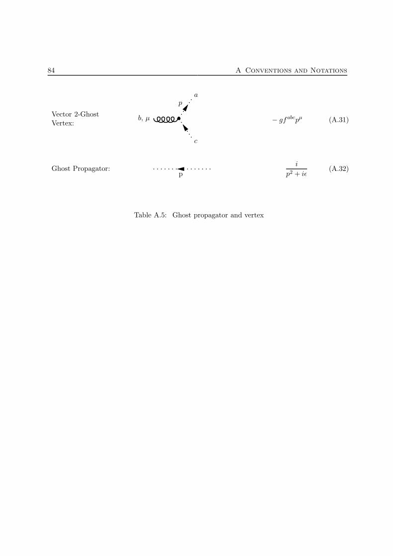
84 A Conventions and Notations
Vector 2-GhostVertex:
p
b, µ
c
a
− gfabcpµ (A.31)
Ghost Propagator:p
i
p2 + iε(A.32)
Table A.5: Ghost propagator and vertex

B Programs and Implementation
B.1 Programs Used in This Thesis
The following list gives an overview of the programs used in this thesis for the generation andevaluation of Feynman topologies, matrix elements and squared amplitudes.
Mathematica: This is a general computing environment which organizes many algorithmic,visualization and user interface capabilities within a document-like user interface paradigm.It can be extended with several packages (e.g. FeynCalc). In contrast to Mathematica ,the packages used here are freely available.Homepage: http://www.wolfram.com
FeynCalc: This is a Mathematica package for algebraic calculations in elementary particlephysics. It is used for frequently occuring tasks such as contraction of Lorentz indices,color factor calculations, Dirac matrix manipulations and traces. The vectors, metrictensors and Dirac matrices can be defined in arbitrary dimensions. It was used for the LO
process qq → t t and the NLO process qq → g t t in DRED.Homepage: http://www.feyncalc.org
FeynArts: This a Mathematica package for the generation and visualization of Feynman dia-grams and amplitudes [33]. It was used to generate the Feynman amplitudes for the LOprocess. Since the available models (such as MSSMQCD.mod) do not comprise an ε scalar, thisparticle with its corresponding couplings is implemented (section B.2). We use FeynCalc,
FeynArts and FormCalc for the LO GG → t t and for the NLO process GG → G t t in
4 dimensions and in DRED. It was also used for the LO process qq → t t and the NLO
process qq → G t t in 4 dimensions.Homepage: http://www.feynarts.de
FormCalc: This is a Mathematica package which calculates and simplifies tree-level and oneloop Feynman diagrams [34]. It accepts diagrams generated with FeynArts and returns theresults for further numerical or analytical evaluation. FormCalc uses Form and Fortran.Homepage: http://www.feynarts.de/formcalc
FeynMF: This is a macro package for LATEX and METAPOST/METAFONT which generatesFeynman diagrams. Aside from the graphs in section C all Feynman diagrams in thiswork were drawn with this program.Homepage: http://theorie.physik.uni-wuerzburg.de/∼ohl
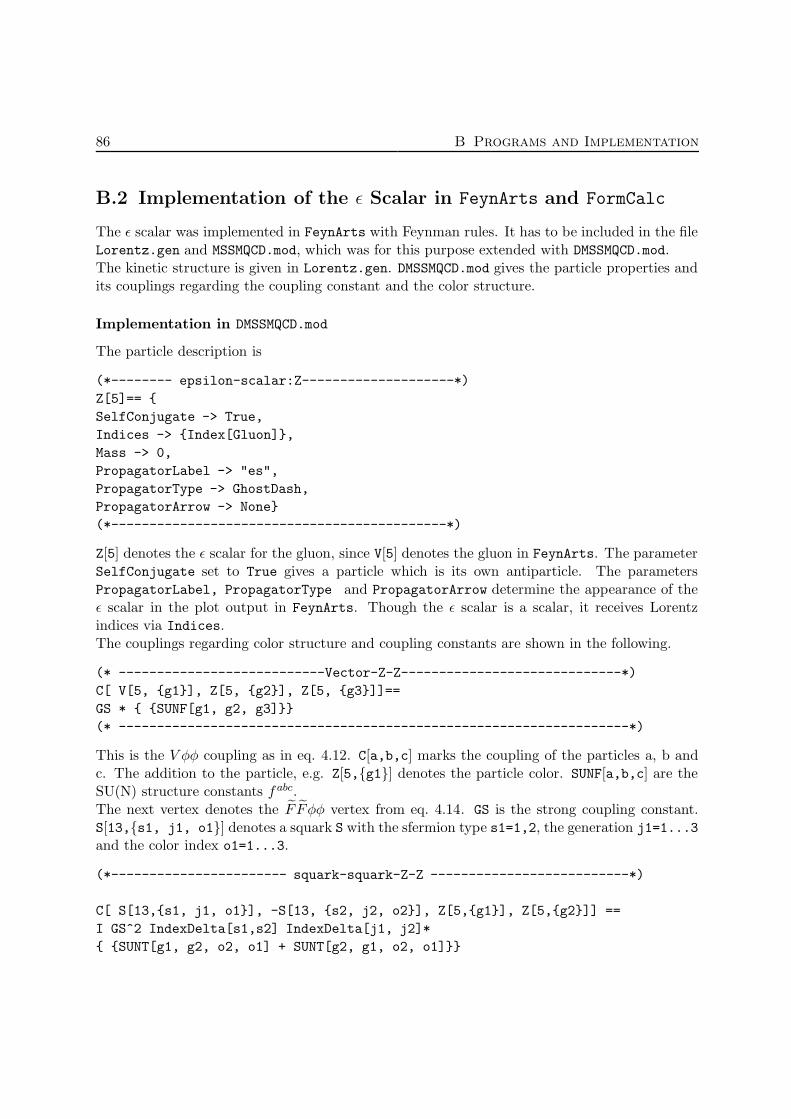
86 B Programs and Implementation
B.2 Implementation of the ε Scalar in FeynArts and FormCalc
The ε scalar was implemented in FeynArts with Feynman rules. It has to be included in the fileLorentz.gen and MSSMQCD.mod, which was for this purpose extended with DMSSMQCD.mod.The kinetic structure is given in Lorentz.gen. DMSSMQCD.mod gives the particle properties andits couplings regarding the coupling constant and the color structure.
Implementation in DMSSMQCD.mod
The particle description is
(*-------- epsilon-scalar:Z--------------------*)
Z[5]== {
SelfConjugate -> True,
Indices -> {Index[Gluon]},
Mass -> 0,
PropagatorLabel -> "es",
PropagatorType -> GhostDash,
PropagatorArrow -> None}
(*--------------------------------------------*)
Z[5] denotes the ε scalar for the gluon, since V[5] denotes the gluon in FeynArts. The parameterSelfConjugate set to True gives a particle which is its own antiparticle. The parametersPropagatorLabel, PropagatorType and PropagatorArrow determine the appearance of theε scalar in the plot output in FeynArts. Though the ε scalar is a scalar, it receives Lorentzindices via Indices.The couplings regarding color structure and coupling constants are shown in the following.
(* ---------------------------Vector-Z-Z-----------------------------*)
C[ V[5, {g1}], Z[5, {g2}], Z[5, {g3}]]==
GS * { {SUNF[g1, g2, g3]}}
(* -------------------------------------------------------------------*)
This is the V φφ coupling as in eq. 4.12. C[a,b,c] marks the coupling of the particles a, b andc. The addition to the particle, e.g. Z[5,{g1}] denotes the particle color. SUNF[a,b,c] are theSU(N) structure constants f abc.The next vertex denotes the F F φφ vertex from eq. 4.14. GS is the strong coupling constant.S[13,{s1, j1, o1}] denotes a squark S with the sfermion type s1=1,2, the generation j1=1...3
and the color index o1=1...3.
(*----------------------- squark-squark-Z-Z --------------------------*)
C[ S[13,{s1, j1, o1}], -S[13, {s2, j2, o2}], Z[5,{g1}], Z[5,{g2}]] ==
I GS^2 IndexDelta[s1,s2] IndexDelta[j1, j2]*
{ {SUNT[g1, g2, o2, o1] + SUNT[g2, g1, o2, o1]}}
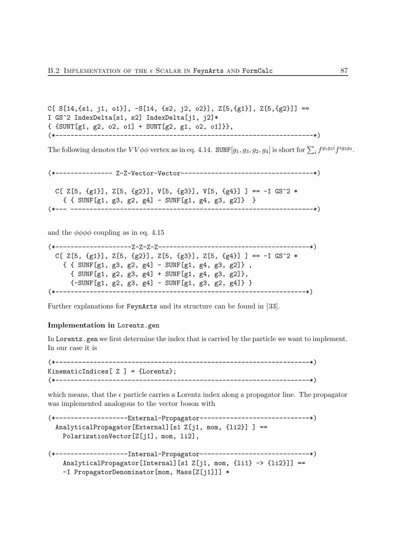
B.2 Implementation of the ε Scalar in FeynArts and FormCalc 87
C[ S[14,{s1, j1, o1}], -S[14, {s2, j2, o2}], Z[5,{g1}], Z[5,{g2}]] ==
I GS^2 IndexDelta[s1, s2] IndexDelta[j1, j2]*
{ {SUNT[g1, g2, o2, o1] + SUNT[g2, g1, o2, o1]}},
(*--------------------------------------------------------------------*)
The following denotes the V V φφ vertex as in eq. 4.14. SUNF[g1, g3, g2, g4] is short for∑
i fg1g3if ig2g4 .
(*--------------- Z-Z-Vector-Vector-----------------------------------*)
C[ Z[5, {g1}], Z[5, {g2}], V[5, {g3}], V[5, {g4}] ] == -I GS^2 *
{ { SUNF[g1, g3, g2, g4] - SUNF[g1, g4, g3, g2]} }
(*--- ----------------------------------------------------------------*)
and the φφφφ coupling as in eq. 4.15
(*--------------------Z-Z-Z-Z----------------------------------------*)
C[ Z[5, {g1}], Z[5, {g2}], Z[5, {g3}], Z[5, {g4}] ] == -I GS^2 *
{ { SUNF[g1, g3, g2, g4] - SUNF[g1, g4, g3, g2]} ,
{ SUNF[g1, g2, g3, g4] + SUNF[g1, g4, g3, g2]},
{-SUNF[g1, g2, g3, g4] - SUNF[g1, g3, g2, g4]} }
(*------------------------------------------------------------------*)
Further explanations for FeynArts and its structure can be found in [33].
Implementation in Lorentz.gen
In Lorentz.genwe first determine the index that is carried by the particle we want to implement.In our case it is
(*-------------------------------------------------------------------*)
KinematicIndices[ Z ] = {Lorentz};
(*-------------------------------------------------------------------*)
which means, that the ε particle carries a Lorentz index along a propagator line. The propagatorwas implemented analogous to the vector boson with
(*-------------------External-Propagator-----------------------------*)
AnalyticalPropagator[External][s1 Z[j1, mom, {li2}] ] ==
PolarizationVector[Z[j1], mom, li2],
(*-------------------Internal-Propagator-----------------------------*)
AnalyticalPropagator[Internal][s1 Z[j1, mom, {li1} -> {li2}]] ==
-I PropagatorDenominator[mom, Mass[Z[j1]]] *

88 B Programs and Implementation
MetricTensor[li1, li2]
(*-------------------------------------------------------------------*)
FeynArts works with Internal and External Propagators. The External Propagator cor-responds to the polarization vectors PolarizationVector[Z[j1], mom, li2] with momentummom and Lorentz index li2. The Internal Propagator changes the Lorentz index li1 to li2
and comes with the same denominator and metric tensor as the gluon.Now we just have to add the kinematical behaviour of the ε scalar for the vertices.
(*-----------------------------V-Z-Z--------------------------------*)
AnalyticalCoupling[ s1 V[j1, mom1, {li1}], s2 Z[j2, mom2, {li2}],
s3 Z[j3, mom3, {li3}] ] ==
G[-1][s1 V[j1], s2 Z[j2], s3 Z[j3]].
{MetricTensor[li2, li3] FourVector[mom3-mom2, li1]},
(*------------------------Z-Z-squark-squark-------------------------*)
AnalyticalCoupling[s1 S[j1, mom1], s2 S[j2, mom2],s3 Z[j3, mom3,
{li3}], s4 Z[j4, mom4, {li4}]]
== G[1][ s1 S[j1], s2 S[j2],s3 Z[j3], s4 Z[j4]].
{MetricTensor[li3, li4]},
(*---------------------------Z-Z-V-V--------------------------------*)
AnalyticalCoupling[ s1 Z[j1, mom1, {li1}], s2 Z[j2, mom2, {li2}],
s3 V[j3, mom3, {li3}], s4 V[j4, mom4, {li4}] ] ==
G[1][s1 Z[j1], s2 Z[j2], s3 V[j3], s4 V[j4]] .
{ MetricTensor[li1, li2] MetricTensor[li3, li4] }
(*---------------v-----------Z-Z-Z-Z--------------------------------*)
AnalyticalCoupling[ s1 Z[j1, mom1, {li1}], s2 Z[j2, mom2, {li2}],
s3 V[j3, mom3, {li3}], s4 V[j4, mom4, {li4}] ] ==
G[1][s1 Z[j1], s2 Z[j2], s3 V[j3], s4 V[j4]] .
{ MetricTensor[li1, li2] MetricTensor[li3, li4] ,
MetricTensor[li1, li3] MetricTensor[li2, li4],
MetricTensor[li1, li4] MetricTensor[li3, li2] }
(*-----------------------------------------------------------------*)
The ε scalars are implemented using the same Lorentz indices as the vector bosons and thedistinction is only made in the polarization sum. This is possible as long as no loops appear inthe calculation.
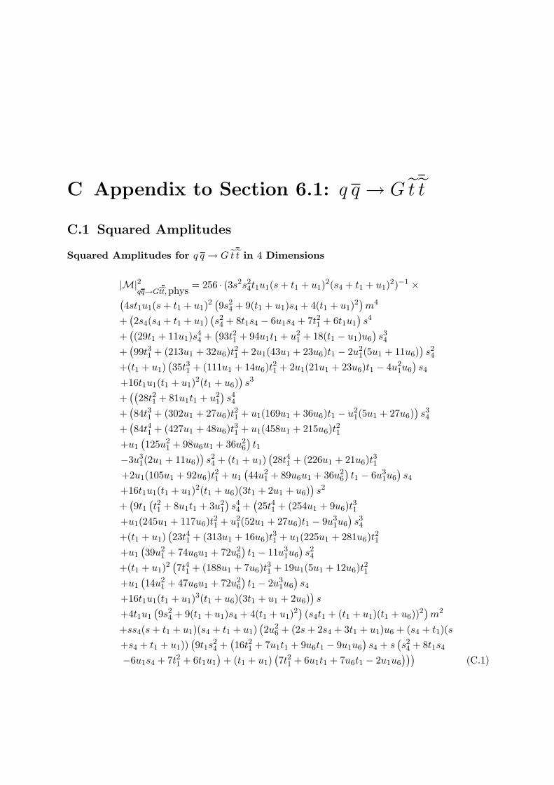
C Appendix to Section 6.1: q q → G t t
C.1 Squared Amplitudes
Squared Amplitudes for q q → G t t in 4 Dimensions
|M|2qq→Getet,phys
= 256 · (3s2s24t1u1(s+ t1 + u1)2(s4 + t1 + u1)
2)−1 ×(4st1u1(s+ t1 + u1)
2(9s24 + 9(t1 + u1)s4 + 4(t1 + u1)
2)m4
+(2s4(s4 + t1 + u1)
(s24 + 8t1s4 − 6u1s4 + 7t21 + 6t1u1
)s4
+((29t1 + 11u1)s
44 +
(93t21 + 94u1t1 + u2
1 + 18(t1 − u1)u6
)s34
+(99t31 + (213u1 + 32u6)t
21 + 2u1(43u1 + 23u6)t1 − 2u2
1(5u1 + 11u6))s24
+(t1 + u1)(35t31 + (111u1 + 14u6)t
21 + 2u1(21u1 + 23u6)t1 − 4u2
1u6
)s4
+16t1u1(t1 + u1)2(t1 + u6)
)s3
+((
28t21 + 81u1t1 + u21
)s44
+(84t31 + (302u1 + 27u6)t
21 + u1(169u1 + 36u6)t1 − u2
1(5u1 + 27u6))s34
+(84t41 + (427u1 + 48u6)t
31 + u1(458u1 + 215u6)t
21
+u1
(125u2
1 + 98u6u1 + 36u26
)t1
−3u31(2u1 + 11u6)
)s24 + (t1 + u1)
(28t41 + (226u1 + 21u6)t
31
+2u1(105u1 + 92u6)t21 + u1
(44u2
1 + 89u6u1 + 36u26
)t1 − 6u3
1u6
)s4
+16t1u1(t1 + u1)2(t1 + u6)(3t1 + 2u1 + u6)
)s2
+(9t1(t21 + 8u1t1 + 3u2
1
)s44 +
(25t41 + (254u1 + 9u6)t
31
+u1(245u1 + 117u6)t21 + u2
1(52u1 + 27u6)t1 − 9u31u6
)s34
+(t1 + u1)(23t41 + (313u1 + 16u6)t
31 + u1(225u1 + 281u6)t
21
+u1
(39u2
1 + 74u6u1 + 72u26
)t1 − 11u3
1u6
)s24
+(t1 + u1)2(7t41 + (188u1 + 7u6)t
31 + 19u1(5u1 + 12u6)t
21
+u1
(14u2
1 + 47u6u1 + 72u26
)t1 − 2u3
1u6
)s4
+16t1u1(t1 + u1)3(t1 + u6)(3t1 + u1 + 2u6)
)s
+4t1u1
(9s24 + 9(t1 + u1)s4 + 4(t1 + u1)
2)(s4t1 + (t1 + u1)(t1 + u6))
2)m2
+ss4(s+ t1 + u1)(s4 + t1 + u1)(2u2
6 + (2s+ 2s4 + 3t1 + u1)u6 + (s4 + t1)(s
+s4 + t1 + u1))(9t1s
24 +
(16t21 + 7u1t1 + 9u6t1 − 9u1u6
)s4 + s
(s24 + 8t1s4
−6u1s4 + 7t21 + 6t1u1
)+ (t1 + u1)
(7t21 + 6u1t1 + 7u6t1 − 2u1u6
)))(C.1)

90 C Appendix to Section 6.1: q q → G t t
Squared Amplitudes for q q → g t t
|M|2qq→getet
= −(3s4st1u1(s4 + t1 + u1)(s+ t1 + u1)2)−1 ×
(4(35u1t
51 + 91u2
1t41 −Ds4st
41 − 2s4st
41 − 28m2u1t
41 + 4Ds4u1t
41 + 82s4u1t
41 + 70su1t
41
+119u1u6t41 + 77u3
1t31 −Ds4s
2t31 − 6s4s2t31 − 28m2u2
1t31 + 12Ds4u
21t
31 + 133s4u
21t
31 + 126su2
1t31
+140u1u26t
31 − 4Ds24st
31 + 26Ds24u1t
31 + 21s24u1t
31 − 64s4m
2u1t31
+35s2u1t31 + 2Ds4su1t
31 + 154s4su1t
31 + 287u2
1u6t31 −Ds4su6t
31
−10s4su6t31 − 28m2u1u6t
31 + 4Ds4u1u6t
31 + 259s4u1u6t
31 + 196su1u
26t
21
+203su1u6t31 + 21u4
1t21 − 4s4s
3t21 + 28m2u31t
21 + 12Ds4u
31t
21
+43s4u31t
21 + 56su3
1t21 + 56u1u
36t
21 − 4Ds24s
2t21 − 8s24s2t21 − 8s4m
2s2t21 + 52Ds24u21t
21 − 40s24u
21t
21
+35s2u21t
21 + 56m2su2
1t21 + 7Ds4su
21t
21 + 173s4su
21t
21 + 308u2
1u26t
21 − 8s4su
26t
21 + 256s4u1u
26t
21
−5Ds34st21 + 6s34st
21 + 40Ds34u1t
21 − 62s34u1t
21 − 36s24m
2u1t21 + 28m2s2u1t
21
+3Ds4s2u1t
21 + 66s4s
2u1t21 + 14Ds24su1t
21 + 74s24su1t
21 − 4Ds4m
2su1t21
−20s4m2su1t
21 + 217u3
1u6t21 − 20s4s
2u6t21 − 28m2u2
1u6t21 + 12Ds4u
21u6t
21
+400s4u21u6t
21 + 336su2
1u6t21 − 3Ds24su6t
21 − 14s24su6t
21 + 22Ds24u1u6t
21
+138s24u1u6t21 − 36s4m
2u1u6t21 + 84s2u1u6t
21 + 28m2su1u6t
21 + 2Ds4su1u6t
21
+361s4su1u6t21 + 28m2u4
1t1 + 4Ds4u41t1 − 8s4u
41t1 − 8s24s
3t1 − 8s4m2s3t1
+26Ds24u31t1 − 52s24u
31t1 + 64s4m
2u31t1 + 56m2su3
1t1 + 4Ds4su31t1 + 31s4su
31t1 + 112u2
1u36t1
+72s4u1u36t1 + 56su1u
36t1 − 5Ds34s
2t1 + 2s34s2t1 − 8s24m
2s2t1 + 40Ds34u21t1
−80s34u21t1 + 36s24m
2u21t1 + 28m2s2u2
1t1 + 4Ds4s2u2
1t1 + 35s4s2u2
1t1 + 30Ds24su21t1 − 5s24su
21t1
+12Ds4m2su2
1t1 − 24s4m2su2
1t1 + 196u31u
26t1 − 8s4s
2u26t1 + 348s4u
21u
26t1
+280su21u
26t1 − 8s24su
26t1 + 108s24u1u
26t1 + 56s2u1u
26t1 + 292s4su1u
26t1 − 2Ds44st1
+4s44st1 + 18Ds44u1t1 − 36s44u1t1 + 4s4s3u1t1 + 13Ds24s
2u1t1 + 7s24s2u1t1
−8s4m2s2u1t1 + 10Ds34su1t1 − 6s34su1t1 − 4Ds24m
2su1t1
−20s24m2su1t1 + 49u4
1u6t1 − 8s4s3u6t1 + 28m2u3
1u6t1
+12Ds4u31u6t1 + 133s4u
31u6t1 + 133su3
1u6t1
−28s24s2u6t1 + 44Ds24u
21u6t1 + 58s24u
21u6t1
+84s2u21u6t1 + 112m2su2
1u6t1 + 7Ds4su21u6t1 + 321s4su
21u6t1
−2Ds34su6t1 − 4s34su6t1 + 18Ds34u1u6t1 + 56m2s2u1u6t1
+128s4s2u1u6t1 + 19Ds24su1u6t1 + 110s24su1u6t1 + 36s4m
2su1u6t1−

C.1 Squared Amplitudes 91
−4s34s3 − 8s24m
2s3 + 12Ds24su31 − 24s24su
31 + 16Ds4m
2su31 − 60s4m
2su31 + 56u3
1u36
+72s4u21u
36 + 56su2
1u36 + 72s4su1u
36 − 2Ds44s
2 + 4s44s2 + 12Ds24s
2u21 − 20s24s
2u21
−20s4m2s2u2
1 + 10Ds34su21 − 20s34su
21 + 16Ds24m
2su21 − 68s24m
2su21
+28u41u
26 + 92s4u
31u
26 + 84su3
1u26 − 8s24s
2u26 + 72s24u
21u
26 + 56s2u2
1u26
+172s4su21u
26 + 80s4s
2u1u26 + 64s24su1u
26 + 4s24s
3u1 + 8s4m2s3u1 + 10Ds34s
2u1
−24s34s2u1 − 44s24m
2s2u1 − 2Ds44su1 + 4s44su1 + 28m2u41u6 + 4Ds4u
41u6
−8s4u41u6 − 8s24s
3u6 + 22Ds24u31u6 − 44s24u
31u6 + 36s4m
2u31u6 + 84m2su3
1u6
+4Ds4su31u6 + 24s4su
31u6 − 8s34s
2u6 + 18Ds34u21u6 − 36s34u
21u6 + 56m2s2u2
1u6
+40s4s2u2
1u6 + 22Ds24su21u6 − 4s24su
21u6 + 108s4m
2su21u6 + 8s4s
3u1u6
+32s24s2u1u6 + 72s4m
2s2u1u6 + 18Ds34su1u6 − 44s34su1u6
))(C.2)
Squared Amplitudes for q q → φ t t
|M|2qq→φetet
= (3st1u1(s+ t1 + u1)2)−1 ×
4(4 −D)(st31 − 4u1t
31 + s2t21 − 8u2
1t21 + 3s4st
21 − 22s4u1t
21 − 3su1t
21
+su6t21 − 4u1u6t
21 − 4u3
1t1 + 3s4s2t1 − 22s4u
21t1 − 4su2
1t1 + 2s24st1 − 18s24u1t1 −4s2u1t1 + 4m2su1t1 − 14s4su1t1 − 8u2
1u6t1 + 2s4su6t1
−18s4u1u6t1 − 3su1u6t1 + 2s24s2 − 16m2su2
1 − 12s4su21 − 12s4s
2u1 + 2s24su1
−4u31u6 − 18s4u
21u6 − 4su2
1u6 − 18s4su1u6
)(C.3)
The Mandelstam variables for 5 external legs are defined in eq. A.4.
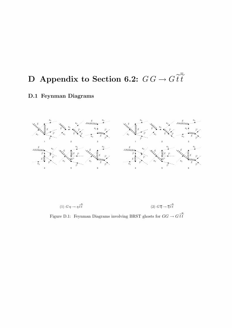
D Appendix to Section 6.2: G G → G t t
D.1 Feynman Diagrams
1
g
ug
ug
t1˜
t1˜
g
2
g
ug
ug
t1˜
t1˜
ug
g
3
g
ug
ug
t1˜
t1˜
ug
g
4
g
ug
ug
t1˜
t1˜
t1˜
g
5
g
ug
ug
t1˜
t1˜
t1˜
g
6
g
ug
ug
t1˜
t1˜
g
g
(1) G η → η et et
1
g
ug
ug
t1˜
t1˜
g
2
g
ug
ug
t1˜
t1˜
ug
g
3
g
ug
ug
t1˜
t1˜
ug
g
4
g
ug
ug
t1˜
t1˜
t1˜
g
5
g
ug
ug
t1˜
t1˜
t1˜
g
6
g
ug
ug
t1˜
t1˜
g
g
(2) G η → η et et
Figure D.1: Feynman Diagrams involving BRST ghosts for GG→ G t t

D.1 Feynman Diagrams 93
1
ug
g
ug
t1˜
t1˜
g
2
ug
g
ug
t1˜
t1˜
ug
g
3
ug
g
ug
t1˜
t1˜
g
t1˜
4
ug
g
ug
t1˜
t1˜
g
t1˜
5
ug
g
ug
t1˜
t1˜
g
g
6
ug
g
ug
t1˜
t1˜
ug
g
(3) η G → η et et
1
ug
g
ug
t1˜
t1˜
g
2
ug
g
ug
t1˜
t1˜
ug
g
3
ug
g
ug
t1˜
t1˜
g
t1˜
4
ug
g
ug
t1˜
t1˜
g
t1˜
5
ug
g
ug
t1˜
t1˜
g
g
6
ug
g
ug
t1˜
t1˜
ug
g
(4) η G → η et et
1
ug
ug
g
t1˜
t1˜
g
2
ug
ug
g
t1˜
t1˜
g
t1˜
3
ug
ug
g
t1˜
t1˜
g
t1˜
4
ug
ug
g
t1˜
t1˜
g
g
5
ug
ug
g
t1˜
t1˜
ug
g
6
ug
ug
g
t1˜
t1˜
ug
g
(5) η η → G et et
1
ug
ug
g
t1˜
t1˜
g
2
ug
ug
g
t1˜
t1˜
g
t1˜
3
ug
ug
g
t1˜
t1˜
g
t1˜
4
ug
ug
g
t1˜
t1˜
g
g
5
ug
ug
g
t1˜
t1˜
ug
g
6
ug
ug
g
t1˜
t1˜
ug
g
(6) η η → G et et
Figure D.2: Feynman Diagrams involving BRST ghosts GG→ G t t

94 D Appendix to Section 6.2: GG→ G t t
1
g
g
g
t1˜
t1˜
g
2
g
g
g
t1˜
t1˜
g
3
g
g
g
t1˜
t1˜
t1˜
4
g
g
g
t1˜
t1˜t1˜
5
g
g
g
t1˜
t1˜
g
6
g
g
g
t1˜
t1˜
t1˜
7
g
g
g
t1˜
t1˜t1˜
8
g
g
g
t1˜
t1˜
t1˜
9
g
g
g
t1˜t1˜
t1˜
10
g
g
g
t1˜
t1˜g
11
g
g
g
t1˜
t1˜
g
t1˜
12
g
g
g
t1˜
t1˜
g
t1˜
13
g
g
g
t1˜
t1˜
g
g
14
g
g
g
t1˜
t1˜
g
t1˜
15
g
g
g
t1˜
t1˜
g
t1˜
16
g
g
g
t1˜
t1˜
g
g
17
g
g
g
t1˜
t1˜
t1˜
g
18
g
g
g
t1˜
t1˜
t1˜
g
19
g
g
g
t1˜
t1˜
g
g
20
g
g
g
t1˜
t1˜
t1˜
t1˜
21
g
g
gt1˜
t1˜t1˜
t1˜
22
g
g
g
t1˜
t1˜
t1˜
t1˜
23
g
g
g
t1˜
t1˜
t1˜
t1˜
24
g
g
g
t1˜
t1˜
t1˜
t1˜
25
g
g
g
t1˜
t1˜t1˜
t1˜
Figure D.3: All 25 graphs for the process GG → G t t. The graphs with number 5, 17, 18, 19contain the propagator which diverges for k2 = k3. The momenta are denoted as infig. 6.4.

D.1 Feynman Diagrams 95
1
es
g
est1˜
t1˜
es
2
es
g
es
t1˜
t1˜
g
3
es
g
es
t1˜
t1˜
es
4
es
g
es
t1˜
t1˜
t1˜
5
es
g
es
t1˜
t1˜t1˜
6
es
g
es
t1˜
t1˜g
7
es
g
es
t1˜
t1˜
es
g
8
es
g
es
t1˜
t1˜
g
t1˜
9
es
g
es
t1˜
t1˜
g
t1˜
10
es
g
es
t1˜
t1˜
g
g
11
es
g
es
t1˜
t1˜
es
g
Figure D.4: φ g → φ t t

96 D Appendix to Section 6.2: GG→ G t t
1
g
es
est1˜
t1˜
es
2
g
es
es
t1˜
t1˜
es
3
g
es
es
t1˜
t1˜
t1˜
4
g
es
es
t1˜
t1˜t1˜
5
g
es
es
t1˜
t1˜
g
6
g
es
es
t1˜
t1˜g
7
g
es
es
t1˜
t1˜
es
g
8
g
es
es
t1˜
t1˜
es
g
9
g
es
es
t1˜
t1˜
t1˜
g
10
g
es
es
t1˜
t1˜
t1˜
g
11
g
es
es
t1˜
t1˜
g
g
Figure D.5: g φ→ φ t t
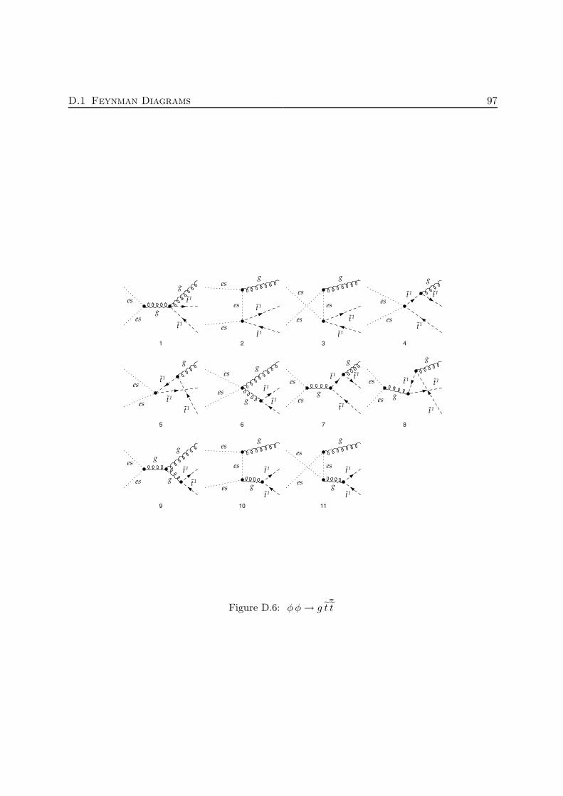
D.1 Feynman Diagrams 97
1
es
es
g
t1˜
t1˜
g
2
es
es
g
t1˜
t1˜
es
3
es
es
g
t1˜
t1˜
es
4
es
es
g
t1˜
t1˜
t1˜
5
es
es
g
t1˜t1˜
t1˜
6
es
es
g
t1˜
t1˜g
7
es
es
g
t1˜
t1˜
g
t1˜
8
es
es
g
t1˜
t1˜
g
t1˜
9
es
es
g
t1˜
t1˜
g
g
10
es
es
g
t1˜
t1˜
es
g
11
es
es
g
t1˜
t1˜
es
g
Figure D.6: φφ→ g t t
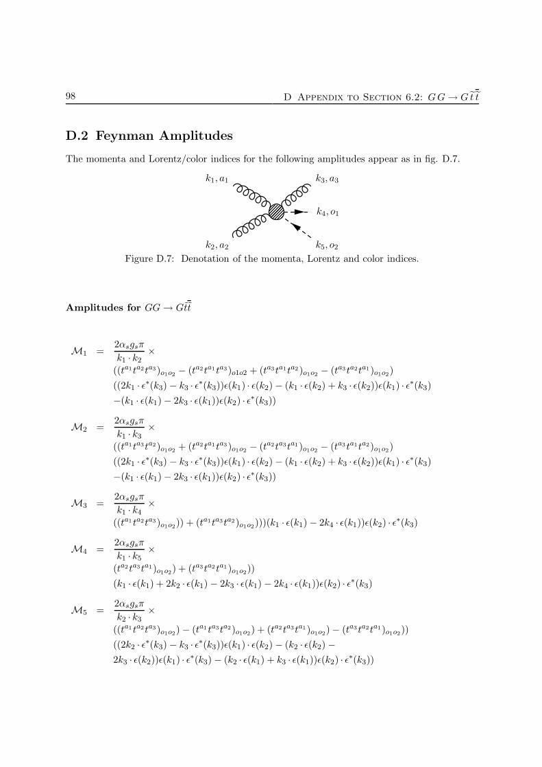
98 D Appendix to Section 6.2: GG→ G t t
D.2 Feynman Amplitudes
The momenta and Lorentz/color indices for the following amplitudes appear as in fig. D.7.
k2, a2
k1, a1
k5, o2
k4, o1
k3, a3
Figure D.7: Denotation of the momenta, Lorentz and color indices.
Amplitudes for GG→ Gtt
M1 =2αsgsπ
k1 · k2×
((ta1ta2ta3)o1o2 − (ta2ta1 ta3)o1o2 + (ta3ta1ta2)o1o2 − (ta3ta2ta1)o1o2)
((2k1 · ε∗(k3) − k3 · ε∗(k3))ε(k1) · ε(k2) − (k1 · ε(k2) + k3 · ε(k2))ε(k1) · ε∗(k3)
−(k1 · ε(k1) − 2k3 · ε(k1))ε(k2) · ε∗(k3))
M2 =2αsgsπ
k1 · k3×
((ta1ta3ta2)o1o2 + (ta2ta1 ta3)o1o2 − (ta2ta3ta1)o1o2 − (ta3 ta1ta2)o1o2)
((2k1 · ε∗(k3) − k3 · ε∗(k3))ε(k1) · ε(k2) − (k1 · ε(k2) + k3 · ε(k2))ε(k1) · ε∗(k3)
−(k1 · ε(k1) − 2k3 · ε(k1))ε(k2) · ε∗(k3))
M3 =2αsgsπ
k1 · k4×
((ta1 ta2ta3)o1o2)) + (ta1ta3ta2)o1o2)))(k1 · ε(k1) − 2k4 · ε(k1))ε(k2) · ε∗(k3)
M4 =2αsgsπ
k1 · k5×
(ta2 ta3ta1)o1o2) + (ta3ta2 ta1)o1o2))
(k1 · ε(k1) + 2k2 · ε(k1) − 2k3 · ε(k1) − 2k4 · ε(k1))ε(k2) · ε∗(k3)
M5 =2αsgsπ
k2 · k3×
((ta1 ta2ta3)o1o2) − (ta1 ta3ta2)o1o2) + (ta2 ta3ta1)o1o2) − (ta3 ta2ta1)o1o2))
((2k2 · ε∗(k3) − k3 · ε∗(k3))ε(k1) · ε(k2) − (k2 · ε(k2) −2k3 · ε(k2))ε(k1) · ε∗(k3) − (k2 · ε(k1) + k3 · ε(k1))ε(k2) · ε∗(k3))
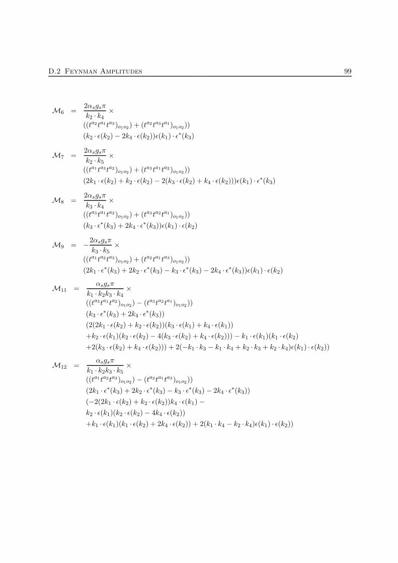
D.2 Feynman Amplitudes 99
M6 =2αsgsπ
k2 · k4×
((ta2 ta1ta3)o1o2) + (ta2 ta3ta1)o1o2))
(k2 · ε(k2) − 2k4 · ε(k2))ε(k1) · ε∗(k3)
M7 =2αsgsπ
k2 · k5×
((ta1 ta3ta2)o1o2) + (ta3 ta1ta2)o1o2))
(2k1 · ε(k2) + k2 · ε(k2) − 2(k3 · ε(k2) + k4 · ε(k2)))ε(k1) · ε∗(k3)
M8 =2αsgsπ
k3 · k4×
((ta3 ta1ta2)o1o2) + (ta3 ta2ta1)o1o2))
(k3 · ε∗(k3) + 2k4 · ε∗(k3))ε(k1) · ε(k2)
M9 = −2αsgsπ
k3 · k5×
((ta1 ta2ta3)o1o2) + (ta2 ta1ta3)o1o2))
(2k1 · ε∗(k3) + 2k2 · ε∗(k3) − k3 · ε∗(k3) − 2k4 · ε∗(k3))ε(k1) · ε(k2)
M11 =αsgsπ
k1 · k2k3 · k4×
((ta3 ta1ta2)o1o2) − (ta3ta2ta1)o1o2))
(k3 · ε∗(k3) + 2k4 · ε∗(k3))
(2(2k1 · ε(k2) + k2 · ε(k2))(k3 · ε(k1) + k4 · ε(k1))
+k2 · ε(k1)(k2 · ε(k2) − 4(k3 · ε(k2) + k4 · ε(k2))) − k1 · ε(k1)(k1 · ε(k2)
+2(k3 · ε(k2) + k4 · ε(k2))) + 2(−k1 · k3 − k1 · k4 + k2 · k3 + k2 · k4)ε(k1) · ε(k2))
M12 =αsgsπ
k1 · k2k3 · k5×
((ta1 ta2ta3)o1o2) − (ta2ta1ta3)o1o2))
(2k1 · ε∗(k3) + 2k2 · ε∗(k3) − k3 · ε∗(k3) − 2k4 · ε∗(k3))
(−2(2k1 · ε(k2) + k2 · ε(k2))k4 · ε(k1) −k2 · ε(k1)(k2 · ε(k2) − 4k4 · ε(k2))
+k1 · ε(k1)(k1 · ε(k2) + 2k4 · ε(k2)) + 2(k1 · k4 − k2 · k4)ε(k1) · ε(k2))
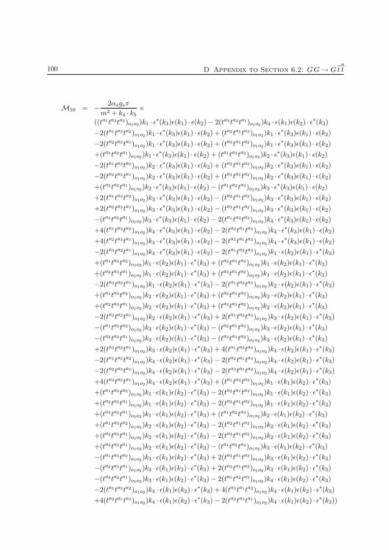
100 D Appendix to Section 6.2: GG→ G t t
M10 = − 2αsgsπ
m2 + k4 · k5×
((ta1ta2ta3)o1o2)k1 · ε∗(k3)ε(k1) · ε(k2) − 2(ta3 ta2ta1)o1o2)k4 · ε(k1)ε(k2) · ε∗(k3)
−2(ta1ta3ta2)o1o2)k1 · ε∗(k3)ε(k1) · ε(k2) + (ta2 ta1ta3)o1o2)k1 · ε∗(k3)ε(k1) · ε(k2)
−2(ta2ta3ta1)o1o2)k1 · ε∗(k3)ε(k1) · ε(k2) + (ta3 ta1ta2)o1o2)k1 · ε∗(k3)ε(k1) · ε(k2)
+(ta3ta2ta1)o1o2)k1 · ε∗(k3)ε(k1) · ε(k2) + (ta1ta2ta3)o1o2)k2 · ε∗(k3)ε(k1) · ε(k2)
−2(ta1ta3ta2)o1o2)k2 · ε∗(k3)ε(k1) · ε(k2) + (ta2 ta1ta3)o1o2)k2 · ε∗(k3)ε(k1) · ε(k2)
−2(ta2ta3ta1)o1o2)k2 · ε∗(k3)ε(k1) · ε(k2) + (ta3 ta1ta2)o1o2)k2 · ε∗(k3)ε(k1) · ε(k2)
+(ta3ta2ta1)o1o2)k2 · ε∗(k3)ε(k1) · ε(k2) − (ta1ta2ta3)o1o2)k3 · ε∗(k3)ε(k1) · ε(k2)
+2(ta1ta3ta2)o1o2)k3 · ε∗(k3)ε(k1) · ε(k2) − (ta2 ta1ta3)o1o2)k3 · ε∗(k3)ε(k1) · ε(k2)
+2(ta2ta3ta1)o1o2)k3 · ε∗(k3)ε(k1) · ε(k2) − (ta3 ta1ta2)o1o2)k3 · ε∗(k3)ε(k1) · ε(k2)
−(ta3ta2ta1)o1o2)k3 · ε∗(k3)ε(k1) · ε(k2) − 2(ta1 ta2ta3)o1o2)k4 · ε∗(k3)ε(k1) · ε(k2)
+4(ta1ta3ta2)o1o2)k4 · ε∗(k3)ε(k1) · ε(k2) − 2(ta2 ta1ta3)o1o2)k4 · ε∗(k3)ε(k1) · ε(k2)
+4(ta2ta3ta1)o1o2)k4 · ε∗(k3)ε(k1) · ε(k2) − 2(ta3 ta1ta2)o1o2)k4 · ε∗(k3)ε(k1) · ε(k2)
−2(ta3ta2ta1)o1o2)k4 · ε∗(k3)ε(k1) · ε(k2) − 2(ta1 ta2ta3)o1o2)k1 · ε(k2)ε(k1) · ε∗(k3)
+(ta1ta3ta2)o1o2)k1 · ε(k2)ε(k1) · ε∗(k3) + (ta2ta1ta3)o1o2)k1 · ε(k2)ε(k1) · ε∗(k3)
+(ta2ta3ta1)o1o2)k1 · ε(k2)ε(k1) · ε∗(k3) + (ta3ta1ta2)o1o2)k1 · ε(k2)ε(k1) · ε∗(k3)
−2(ta3ta2ta1)o1o2)k1 · ε(k2)ε(k1) · ε∗(k3) − 2(ta1 ta2ta3)o1o2)k2 · ε(k2)ε(k1) · ε∗(k3)
+(ta1ta3ta2)o1o2)k2 · ε(k2)ε(k1) · ε∗(k3) + (ta2ta1ta3)o1o2)k2 · ε(k2)ε(k1) · ε∗(k3)
+(ta2ta3ta1)o1o2)k2 · ε(k2)ε(k1) · ε∗(k3) + (ta3ta1ta2)o1o2)k2 · ε(k2)ε(k1) · ε∗(k3)
−2(ta3ta2ta1)o1o2)k2 · ε(k2)ε(k1) · ε∗(k3) + 2(ta1 ta2ta3)o1o2)k3 · ε(k2)ε(k1) · ε∗(k3)
−(ta1ta3ta2)o1o2)k3 · ε(k2)ε(k1) · ε∗(k3) − (ta2ta1ta3)o1o2)k3 · ε(k2)ε(k1) · ε∗(k3)
−(ta2ta3ta1)o1o2)k3 · ε(k2)ε(k1) · ε∗(k3) − (ta3ta1ta2)o1o2)k3 · ε(k2)ε(k1) · ε∗(k3)
+2(ta3ta2ta1)o1o2)k3 · ε(k2)ε(k1) · ε∗(k3) + 4(ta1 ta2ta3)o1o2)k4 · ε(k2)ε(k1) · ε∗(k3)
−2(ta1ta3ta2)o1o2)k4 · ε(k2)ε(k1) · ε∗(k3) − 2(ta2 ta1ta3)o1o2)k4 · ε(k2)ε(k1) · ε∗(k3)
−2(ta2ta3ta1)o1o2)k4 · ε(k2)ε(k1) · ε∗(k3) − 2(ta3 ta1ta2)o1o2)k4 · ε(k2)ε(k1) · ε∗(k3)
+4(ta3ta2ta1)o1o2)k4 · ε(k2)ε(k1) · ε∗(k3) + (ta1 ta2ta3)o1o2)k1 · ε(k1)ε(k2) · ε∗(k3)
+(ta1ta3ta2)o1o2)k1 · ε(k1)ε(k2) · ε∗(k3) − 2(ta2 ta1ta3)o1o2)k1 · ε(k1)ε(k2) · ε∗(k3)
+(ta2ta3ta1)o1o2)k1 · ε(k1)ε(k2) · ε∗(k3) − 2(ta3 ta1ta2)o1o2)k1 · ε(k1)ε(k2) · ε∗(k3)
+(ta3ta2ta1)o1o2)k1 · ε(k1)ε(k2) · ε∗(k3) + (ta1ta2ta3)o1o2)k2 · ε(k1)ε(k2) · ε∗(k3)
+(ta1ta3ta2)o1o2)k2 · ε(k1)ε(k2) · ε∗(k3) − 2(ta2 ta1ta3)o1o2)k2 · ε(k1)ε(k2) · ε∗(k3)
+(ta2ta3ta1)o1o2)k2 · ε(k1)ε(k2) · ε∗(k3) − 2(ta3 ta1ta2)o1o2)k2 · ε(k1)ε(k2) · ε∗(k3)
+(ta3ta2ta1)o1o2)k2 · ε(k1)ε(k2) · ε∗(k3) − (ta1ta2ta3)o1o2)k3 · ε(k1)ε(k2) · ε∗(k3)
−(ta1ta3ta2)o1o2)k3 · ε(k1)ε(k2) · ε∗(k3) + 2(ta2 ta1ta3)o1o2)k3 · ε(k1)ε(k2) · ε∗(k3)
−(ta2ta3ta1)o1o2)k3 · ε(k1)ε(k2) · ε∗(k3) + 2(ta3 ta1ta2)o1o2)k3 · ε(k1)ε(k2) · ε∗(k3)
−(ta3ta2ta1)o1o2)k3 · ε(k1)ε(k2) · ε∗(k3) − 2(ta1 ta2ta3)o1o2)k4 · ε(k1)ε(k2) · ε∗(k3)
−2(ta1ta3ta2)o1o2)k4 · ε(k1)ε(k2) · ε∗(k3) + 4(ta3 ta1ta2)o1o2)k4 · ε(k1)ε(k2) · ε∗(k3)
+4(ta2ta1ta3)o1o2)k4 · ε(k1)ε(k2) · ε∗(k3) − 2(ta2 ta3ta1)o1o2)k4 · ε(k1)ε(k2) · ε∗(k3))
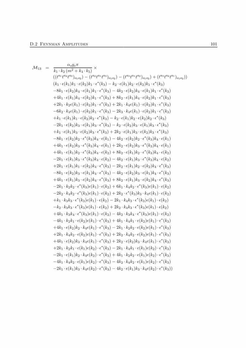
D.2 Feynman Amplitudes 101
M13 =αsgsπ
k1 · k2 (m2 + k4 · k5)×
((ta1 ta2ta3)o1o2) − (ta2ta1ta3)o1o2) − (ta3ta1ta2)o1o2) + (ta3 ta2ta1)o1o2))
(k1 · ε(k1)k1 · ε(k2)k1 · ε∗(k3) − k2 · ε(k1)k2 · ε(k2)k1 · ε∗(k3)
−8k1 · ε(k2)k4 · ε(k1)k1 · ε∗(k3) − 4k2 · ε(k2)k4 · ε(k1)k1 · ε∗(k3)
+4k1 · ε(k1)k4 · ε(k2)k1 · ε∗(k3) + 8k2 · ε(k1)k4 · ε(k2)k1 · ε∗(k3)
+2k1 · k2ε(k1) · ε(k2)k1 · ε∗(k3) + 2k1 · k4ε(k1) · ε(k2)k1 · ε∗(k3)
−6k2 · k4ε(k1) · ε(k2)k1 · ε∗(k3) − 2k3 · k4ε(k1) · ε(k2)k1 · ε∗(k3)
+k1 · ε(k1)k1 · ε(k2)k2 · ε∗(k3) − k2 · ε(k1)k2 · ε(k2)k2 · ε∗(k3)
−2k1 · ε(k2)k3 · ε(k1)k3 · ε∗(k3) − k2 · ε(k2)k3 · ε(k1)k3 · ε∗(k3)
+k1 · ε(k1)k3 · ε(k2)k3 · ε∗(k3) + 2k2 · ε(k1)k3 · ε(k2)k3 · ε∗(k3)
−8k1 · ε(k2)k2 · ε∗(k3)k4 · ε(k1) − 4k2 · ε(k2)k2 · ε∗(k3)k4 · ε(k1)
+4k1 · ε(k2)k3 · ε∗(k3)k4 · ε(k1) + 2k2 · ε(k2)k3 · ε∗(k3)k4 · ε(k1)
+4k1 · ε(k1)k2 · ε∗(k3)k4 · ε(k2) + 8k2 · ε(k1)k2 · ε∗(k3)k4 · ε(k2)
−2k1 · ε(k1)k3 · ε∗(k3)k4 · ε(k2) − 4k2 · ε(k1)k3 · ε∗(k3)k4 · ε(k2)
+2k1 · ε(k1)k1 · ε(k2)k4 · ε∗(k3) − 2k2 · ε(k1)k2 · ε(k2)k4 · ε∗(k3)
−8k1 · ε(k2)k3 · ε(k1)k4 · ε∗(k3) − 4k2 · ε(k2)k3 · ε(k1)k4 · ε∗(k3)
+4k1 · ε(k1)k3 · ε(k2)k4 · ε∗(k3) + 8k2 · ε(k1)k3 · ε(k2)k4 · ε∗(k3)
−2k1 · k2k2 · ε∗(k3)ε(k1) · ε(k2) + 6k1 · k4k2 · ε∗(k3)ε(k1) · ε(k2)
−2k2 · k4k2 · ε∗(k3)ε(k1) · ε(k2) + 2k2 · ε∗(k3)k3 · k4ε(k1) · ε(k2)
+k1 · k3k3 · ε∗(k3)ε(k1) · ε(k2) − 2k1 · k4k3 · ε∗(k3)ε(k1) · ε(k2)
−k2 · k3k3 · ε∗(k3)ε(k1) · ε(k2) + 2k2 · k4k3 · ε∗(k3)ε(k1) · ε(k2)
+4k1 · k3k4 · ε∗(k3)ε(k1) · ε(k2) − 4k2 · k3k4 · ε∗(k3)ε(k1) · ε(k2)
−4k1 · k2k1 · ε(k2)ε(k1) · ε∗(k3) + 4k1 · k4k1 · ε(k2)ε(k1) · ε∗(k3)
+4k1 · ε(k2)k2 · k4ε(k1) · ε∗(k3) − 2k1 · k2k2 · ε(k2)ε(k1) · ε∗(k3)
+2k1 · k4k2 · ε(k2)ε(k1) · ε∗(k3) + 2k2 · k4k2 · ε(k2)ε(k1) · ε∗(k3)
+4k1 · ε(k2)k3 · k4ε(k1) · ε∗(k3) + 2k2 · ε(k2)k3 · k4ε(k1) · ε∗(k3)
+2k1 · k2k1 · ε(k1)ε(k2) · ε∗(k3) − 2k1 · k4k1 · ε(k1)ε(k2) · ε∗(k3)
−2k1 · ε(k1)k2 · k4ε(k2) · ε∗(k3) + 4k1 · k2k2 · ε(k1)ε(k2) · ε∗(k3)
−4k1 · k4k2 · ε(k1)ε(k2) · ε∗(k3) − 4k2 · k4k2 · ε(k1)ε(k2) · ε∗(k3)
−2k1 · ε(k1)k3 · k4ε(k2) · ε∗(k3) − 4k2 · ε(k1)k3 · k4ε(k2) · ε∗(k3))

102 D Appendix to Section 6.2: GG→ G t t
M14 =αsgsπ
k1 · k3k2 · k4×
((ta2 ta1ta3)o1o2) − (ta2ta3ta1)o1o2))
(k2 · ε(k2) − 2k4 · ε(k2))(k1 · ε(k1)k1 · ε∗(k3) + 2k3 · k4ε(k1) · ε∗(k3)
+4k2 · ε(k1)k1 · ε∗(k3) − 4k4 · ε(k1)k1 · ε∗(k3) − 2k1 · ε(k1)k2 · ε∗(k3)
+4k2 · ε∗(k3)k3 · ε(k1) − 2k2 · ε(k1)k3 · ε∗(k3) − k3 · ε(k1)k3 · ε∗(k3)
+2k3 · ε∗(k3)k4 · ε(k1) + 2k1 · ε(k1)k4 · ε∗(k3) − 4k3 · ε(k1)k4 · ε∗(k3)
−2k1 · k2ε(k1) · ε∗(k3) + 2k1 · k4ε(k1) · ε∗(k3) − 2k2 · k3ε(k1) · ε∗(k3))
M15 = − αsgsπ
k1 · k3k2 · k5((ta1ta3ta2)o1o2 − (ta3 ta1ta2)o1o2) ×
(2k1 · ε(k2) + k2 · ε(k2) − 2k3 · ε(k2) − 2k4 · ε(k2))
(−k1 · ε(k1)k1 · ε∗(k3) + 4k4 · ε(k1)k1 · ε∗(k3) + k3 · ε(k1)k3 · ε∗(k3)
−2k3 · ε∗(k3)k4 · ε(k1) − 2k1 · ε(k1)k4 · ε∗(k3) + 4k3 · ε(k1)k4 · ε∗(k3)
−2k1 · k4ε(k1) · ε∗(k3) − 2k3 · k4ε(k1) · ε∗(k3))
M17 = − αsgsπ
k1 · k4k2 · k3((ta1ta2ta3)o1o2 − (ta1 ta3ta2)o1o2) ×
(k1 · ε(k1) − 2k4 · ε(k1))
(2k1 · ε∗(k3)k2 · ε(k2) − k2 · ε∗(k3)k2 · ε(k2) − 2k4 · ε∗(k3)k2 · ε(k2)
−4k1 · ε(k2)k2 · ε∗(k3) − 4k1 · ε∗(k3)k3 · ε(k2) + 2k1 · ε(k2)k3 · ε∗(k3)
+k3 · ε(k2)k3 · ε∗(k3) + 4k2 · ε∗(k3)k4 · ε(k2) − 2k3 · k4ε(k2) · ε∗(k3)
−2k3 · ε∗(k3)k4 · ε(k2) + 4k3 · ε(k2)k4 · ε∗(k3) + 2k1 · k2ε(k2) · ε∗(k3)
+2k1 · k3ε(k2) · ε∗(k3) − 2k2 · k4ε(k2) · ε∗(k3))
M18 = − αsgsπ
k1 · k5k2 · k3×
(ta2 ta3ta1)o1o2 − (ta3ta2ta1)o1o2
(k1 · ε(k1) + 2k2 · ε(k1) − 2k3 · ε(k1) − 2k4 · ε(k1))
(−k2 · ε(k2)k2 · ε∗(k3) + 4k4 · ε(k2)k2 · ε∗(k3)
+k3 · ε(k2)k3 · ε∗(k3) − 2k3 · ε∗(k3)k4 · ε(k2) − 2k2 · ε(k2)k4 · ε∗(k3)
+4k3 · ε(k2)k4 · ε∗(k3) − 2k2 · k4ε(k2) · ε∗(k3) − 2k3 · k4ε(k2) · ε∗(k3))
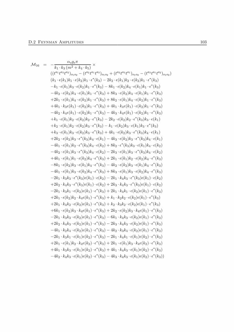
D.2 Feynman Amplitudes 103
M16 = − αsgsπ
k1 · k3 (m2 + k4 · k5)×
((ta1ta3ta2)o1o2 − (ta2 ta1ta3)o1o2 + (ta2ta3ta1)o1o2 − (ta3 ta1ta2)o1o2)
(k1 · ε(k1)k1 · ε(k2)k1 · ε∗(k3) − 2k2 · ε(k1)k2 · ε(k2)k1 · ε∗(k3)
−k1 · ε(k1)k3 · ε(k2)k1 · ε∗(k3) − 8k1 · ε(k2)k4 · ε(k1)k1 · ε∗(k3)
−4k2 · ε(k2)k4 · ε(k1)k1 · ε∗(k3) + 8k3 · ε(k2)k4 · ε(k1)k1 · ε∗(k3)
+2k1 · ε(k1)k4 · ε(k2)k1 · ε∗(k3) + 8k2 · ε(k1)k4 · ε(k2)k1 · ε∗(k3)
+4k1 · k3ε(k1) · ε(k2)k1 · ε∗(k3) + 4k1 · k4ε(k1) · ε(k2)k1 · ε∗(k3)
−4k2 · k4ε(k1) · ε(k2)k1 · ε∗(k3) − 4k3 · k4ε(k1) · ε(k2)k1 · ε∗(k3)
+k1 · ε(k1)k2 · ε(k2)k2 · ε∗(k3) − 2k2 · ε(k2)k2 · ε∗(k3)k3 · ε(k1)
+k2 · ε(k1)k2 · ε(k2)k3 · ε∗(k3) − k1 · ε(k2)k3 · ε(k1)k3 · ε∗(k3)
+k3 · ε(k1)k3 · ε(k2)k3 · ε∗(k3) + 4k1 · ε(k2)k3 · ε∗(k3)k4 · ε(k1)
+2k2 · ε(k2)k3 · ε∗(k3)k4 · ε(k1) − 4k3 · ε(k2)k3 · ε∗(k3)k4 · ε(k1)
−4k1 · ε(k1)k2 · ε∗(k3)k4 · ε(k2) + 8k2 · ε∗(k3)k3 · ε(k1)k4 · ε(k2)
−4k2 · ε(k1)k3 · ε∗(k3)k4 · ε(k2) − 2k3 · ε(k1)k3 · ε∗(k3)k4 · ε(k2)
+4k1 · ε(k1)k1 · ε(k2)k4 · ε∗(k3) + 2k1 · ε(k1)k2 · ε(k2)k4 · ε∗(k3)
−8k1 · ε(k2)k3 · ε(k1)k4 · ε∗(k3) − 4k2 · ε(k2)k3 · ε(k1)k4 · ε∗(k3)
−4k1 · ε(k1)k3 · ε(k2)k4 · ε∗(k3) + 8k3 · ε(k1)k3 · ε(k2)k4 · ε∗(k3)
−2k1 · k3k3 · ε∗(k3)ε(k1) · ε(k2) − 2k1 · k4k3 · ε∗(k3)ε(k1) · ε(k2)
+2k2 · k4k3 · ε∗(k3)ε(k1) · ε(k2) + 2k3 · k4k3 · ε∗(k3)ε(k1) · ε(k2)
−2k1 · k3k1 · ε(k2)ε(k1) · ε∗(k3) + 2k1 · k4k1 · ε(k2)ε(k1) · ε∗(k3)
+2k1 · ε(k2)k2 · k4ε(k1) · ε∗(k3) + k1 · k2k2 · ε(k2)ε(k1) · ε∗(k3)
+2k1 · k4k2 · ε(k2)ε(k1) · ε∗(k3) + k2 · k3k2 · ε(k2)ε(k1) · ε∗(k3)
+6k1 · ε(k2)k3 · k4ε(k1) · ε∗(k3) + 2k2 · ε(k2)k3 · k4ε(k1) · ε∗(k3)
−2k1 · k3k3 · ε(k2)ε(k1) · ε∗(k3) − 6k1 · k4k3 · ε(k2)ε(k1) · ε∗(k3)
+2k2 · k4k3 · ε(k2)ε(k1) · ε∗(k3) − 2k3 · k4k3 · ε(k2)ε(k1) · ε∗(k3)
−4k1 · k2k4 · ε(k2)ε(k1) · ε∗(k3) − 4k2 · k3k4 · ε(k2)ε(k1) · ε∗(k3)
−2k1 · k3k1 · ε(k1)ε(k2) · ε∗(k3) − 2k1 · k4k1 · ε(k1)ε(k2) · ε∗(k3)
+2k1 · ε(k1)k2 · k4ε(k2) · ε∗(k3) + 2k1 · ε(k1)k3 · k4ε(k2) · ε∗(k3)
+4k1 · k3k3 · ε(k1)ε(k2) · ε∗(k3) + 4k1 · k4k3 · ε(k1)ε(k2) · ε∗(k3)
−4k2 · k4k3 · ε(k1)ε(k2) · ε∗(k3) − 4k3 · k4k3 · ε(k1)ε(k2) · ε∗(k3))
104 D Appendix to Section 6.2: GG→ G t t
M19 = − αsgsπ
k2 · k3 (m2 + k4 · k5)×
((ta1ta2ta3)o1o2 − (ta1 ta3ta2)o1o2 − (ta2ta3ta1)o1o2 + (ta3 ta2ta1)o1o2)
(−k1 · ε(k1)k1 · ε∗(k3)k2 · ε(k2) − k2 · ε(k1)k2 · ε∗(k3)k2 · ε(k2)
+k2 · ε∗(k3)k3 · ε(k1)k2 · ε(k2) + 4k1 · ε∗(k3)k4 · ε(k1)k2 · ε(k2)
−2k2 · ε∗(k3)k4 · ε(k1)k2 · ε(k2) − 2k1 · ε(k1)k4 · ε∗(k3)k2 · ε(k2)
−4k2 · ε(k1)k4 · ε∗(k3)k2 · ε(k2) + 4k3 · ε(k1)k4 · ε∗(k3)k2 · ε(k2)
−2k1 · k4ε(k1) · ε∗(k3)k2 · ε(k2) + 2k2 · k3ε(k1) · ε∗(k3)k2 · ε(k2)
+2k2 · k4ε(k1) · ε∗(k3)k2 · ε(k2) − 2k3 · k4ε(k1) · ε∗(k3)k2 · ε(k2)
+2k1 · ε(k1)k1 · ε(k2)k2 · ε∗(k3) + 2k1 · ε(k1)k1 · ε∗(k3)k3 · ε(k2)
−k1 · ε(k1)k1 · ε(k2)k3 · ε∗(k3) + k2 · ε(k1)k3 · ε(k2)k3 · ε∗(k3)
−k3 · ε(k1)k3 · ε(k2)k3 · ε∗(k3) − 8k1 · ε(k2)k2 · ε∗(k3)k4 · ε(k1)
−8k1 · ε∗(k3)k3 · ε(k2)k4 · ε(k1) + 4k1 · ε(k2)k3 · ε∗(k3)k4 · ε(k1)
+2k3 · ε(k2)k3 · ε∗(k3)k4 · ε(k1) + 4k1 · ε(k1)k2 · ε∗(k3)k4 · ε(k2)
+8k2 · ε(k1)k2 · ε∗(k3)k4 · ε(k2) − 8k2 · ε∗(k3)k3 · ε(k1)k4 · ε(k2)
−2k1 · ε(k1)k3 · ε∗(k3)k4 · ε(k2) − 4k2 · ε(k1)k3 · ε∗(k3)k4 · ε(k2)
+4k3 · ε(k1)k3 · ε∗(k3)k4 · ε(k2) + 4k1 · ε(k1)k3 · ε(k2)k4 · ε∗(k3)
+8k2 · ε(k1)k3 · ε(k2)k4 · ε∗(k3) − 8k3 · ε(k1)k3 · ε(k2)k4 · ε∗(k3)
+4k1 · k4k2 · ε∗(k3)ε(k1) · ε(k2) − 4k2 · k3k2 · ε∗(k3)ε(k1) · ε(k2)
−4k2 · k4k2 · ε∗(k3)ε(k1) · ε(k2) + 4k2 · ε∗(k3)k3 · k4ε(k1) · ε(k2)
−2k1 · k4k3 · ε∗(k3)ε(k1) · ε(k2) + 2k2 · k3k3 · ε∗(k3)ε(k1) · ε(k2)
+2k2 · k4k3 · ε∗(k3)ε(k1) · ε(k2) − 2k3 · k4k3 · ε∗(k3)ε(k1) · ε(k2)
+4k1 · k4k3 · ε(k2)ε(k1) · ε∗(k3) − 4k2 · k3k3 · ε(k2)ε(k1) · ε∗(k3)
−4k2 · k4k3 · ε(k2)ε(k1) · ε∗(k3) + 4k3 · k4k3 · ε(k2)ε(k1) · ε∗(k3)
−k1 · k2k1 · ε(k1)ε(k2) · ε∗(k3) − k1 · k3k1 · ε(k1)ε(k2) · ε∗(k3)
−2k1 · ε(k1)k2 · k4ε(k2) · ε∗(k3) − 2k1 · k4k2 · ε(k1)ε(k2) · ε∗(k3)
+2k2 · k3k2 · ε(k1)ε(k2) · ε∗(k3) − 2k2 · k4k2 · ε(k1)ε(k2) · ε∗(k3)
−2k1 · ε(k1)k3 · k4ε(k2) · ε∗(k3) − 6k2 · ε(k1)k3 · k4ε(k2) · ε∗(k3)
−2k1 · k4k3 · ε(k1)ε(k2) · ε∗(k3) + 2k2 · k3k3 · ε(k1)ε(k2) · ε∗(k3)
+6k2 · k4k3 · ε(k1)ε(k2) · ε∗(k3) + 2k3 · k4k3 · ε(k1)ε(k2) · ε∗(k3)
+4k1 · k2k4 · ε(k1)ε(k2) · ε∗(k3) + 4k1 · k3k4 · ε(k1)ε(k2) · ε∗(k3))
M20 =αsgsπ
k1 · k4k2 · k5(ta1ta3ta2)o1o2 ×
(k1 · ε(k1) − 2k4 · ε(k1))(2k1 · ε(k2) + k2 · ε(k2) − 2k3 · ε(k2) − 2k4 · ε(k2))
(2k1 · ε∗(k3) − k3 · ε∗(k3) − 2k4 · ε∗(k3))

D.2 Feynman Amplitudes 105
M21 = − αsgsπ
k1 · k4k3 · k5(ta1 ta2ta3)o1o2 ×
(k1 · ε(k1) − 2k4 · ε(k1))(2k1 · ε(k2) + k2 · ε(k2) − 2k4 · ε(k2))
(2k1 · ε∗(k3) + 2k2 · ε∗(k3) − k3 · ε∗(k3) − 2k4 · ε∗(k3))
M22 =αsgsπ
k1 · k5k2 · k4(ta2ta3ta1)o1o2 ×
(k1 · ε(k1) + 2k2 · ε(k1) − 2k3 · ε(k1) − 2k4 · ε(k1))(k2 · ε(k2) − 2k4 · ε(k2))
(2k2 · ε∗(k3) − k3 · ε∗(k3) − 2k4 · ε∗(k3))
M23 = − αsgsπ
k2 · k4k3 · k5(ta2 ta1ta3)o1o2 ×
(k1 · ε(k1) + 2k2 · ε(k1) − 2k4 · ε(k1))(k2 · ε(k2) − 2k4 · ε(k2))
(2k1 · ε∗(k3) + 2k2 · ε∗(k3) − k3 · ε∗(k3) − 2k4 · ε∗(k3))
M24 =αsgsπ
k1 · k5k3 · k4(ta3ta2ta1)o1o2 ×
(k1 · ε(k1) + 2k2 · ε(k1) − 2k3 · ε(k1) − 2k4 · ε(k1))(k2 · ε(k2) − 2k3 · ε(k2) − 2k4 · ε(k2))
(k3 · ε∗(k3) + 2k4 · ε∗(k3))
M25 =αsgsπ
k2 · k5k3 · k4(ta3ta1ta2)o1o2 ×
(k1 · ε(k1) − 2k3 · ε(k1) − 2k4 · ε(k1))(2k1 · ε(k2) + k2 · ε(k2) − 2k3 · ε(k2) − 2k4 · ε(k2))
(k3 · ε∗(k3) + 2k4 · ε∗(k3))
106 D Appendix to Section 6.2: GG→ G t t
Amplitudes for GG→ Gtt, Ghosts
Mηη→getet
= αsgsπ ((ta1 ta3ta2)o1o2
k1 · k3k2 · k3 (m2 + p1 · p2)×
((ε∗(k3) · k1 − ε∗(k3) · k3)k2 · k3(k1 · k2 − k2 · k3 − 2k2 · p1)
+ε∗(k3) · k2k1 · k3(−k1 · k2 + k1 · k3 + 2(k2 · k3 + k2 · p1 − k3 · p1)))
+(ta2ta3ta1)o1o2
k1 · k3k2 · k3 (m2 + p1 · p2)((ε∗(k3) · k1 − ε∗(k3) · k3)k2 · k3(k1 · k2 − k2 · k3 − 2k2 · p1)
+ε∗(k3) · k2k1 · k3(−k1 · k2 + k1 · k3 + 2(k2 · k3 + k2 · p1 − k3 · p1)))
+(ta2 ta1ta3)o1o2
(−2ε∗(k3) · k2
k1 · k2
+(2ε∗(k3) · k1 + 2ε∗(k3) · k2 − ε∗(k3) · k3 − 2ε∗(k3) · p1)(k1 · k2 − 2k2 · p1)
k1 · k2k3 · p2
−(ε∗(k3) · k1 − ε∗(k3) · k3)(k1 · k2 − k2 · k3 − 2k2 · p1)
k1 · k3 (m2 + p1 · p2)
+1
k1 · k2 (m2 + p1 · p2)(2ε∗(k3) · p1(k1 · k2 − 2k2 · k3) + ε∗(k3) · k1(k1 · k2 − 4k2 · p1)
−ε∗(k3) · k3(k2 · k3 − 2k2 · p1) − ε∗(k3) · k2(k1 · k2 − 2(k1 · p1 − k2 · p1 + k3 · p1))) )
− (ta3 ta2ta1)o1o2
k1 · k2k2 · k3k3 · p1 (m2 + p1 · p2)
(2ε∗(k3) · p1k2 · k3
(−2k2 · p1
(m2 + p1 · p2
)
+k1 · k2
(m2 + k3 · p1 + p1 · p2
)− 2k2 · k3
(m2 + k3 · p1 + p1 · p2
))
+ε∗(k3) · k3k2 · k3
(k1 · k2
(m2 + p1 · p2
)− 2k2 · p1
(m2 − k3 · p1 + p1 · p2
)
−k2 · k3
(k3 · p1 + 2
(m2 + p1 · p2
)))+ k3 · p1 (ε∗(k3) · k1k2 · k3(k1 · k2 − 4k2 · p1)
+ε∗(k3) · k2
(−(k1 · k2)
2 + (k1 · k3 + k2 · k3 + 2k2 · p1 − 2k3 · p1)k1 · k2
+2k2 · k3
(m2 + k1 · p1 − k2 · p1 + k3 · p1 + p1 · p2
))))
+(ta3 ta1ta2)o1o2
k1 · k2k1 · k3k3 · p1 (m2 + p1 · p2)
(2ε∗(k3) · p1k1 · k3
(−2k2 · p1
(m2 + p1 · p2
)
+k1 · k2
(m2 + k3 · p1 + p1 · p2
)− 2k2 · k3
(m2 + k3 · p1 + p1 · p2
))
+k3 · p1
(ε∗(k3) · k1
(−(k1 · k2)
2 + (k1 · k3 + k2 · k3 + 2k2 · p1)k1 · k2 − 4k1 · k3k2 · p1
)
+ε∗(k3) · k2k1 · k3
(2(m2 + k1 · p1 − k2 · p1 + k3 · p1 + p1 · p2
)− k1 · k2
))
+ε∗(k3) · k3
(k3 · p1(k1 · k2)
2 +(k1 · k3
(m2 + p1 · p2
)− (k2 · k3 + 2k2 · p1)k3 · p1
)k1 · k2
−k1 · k3
(2k2 · p1
(m2 − k3 · p1 + p1 · p2
)+ k2 · k3
(k3 · p1 + 2
(m2 + p1 · p2
)))))
+(ta1 ta2ta3)o1o2
k1 · k2k2 · k3k3 · p2 (m2 + p1 · p2)
(ε∗(k3) · k1k2 · k3
(4k2 · p1
(m2 + k3 · p2 + p1 · p2
)
−k1 · k2
(k3 · p2 + 2
(m2 + p1 · p2
)))+ ε∗(k3) · k2
(k3 · p2(k1 · k2)
2−

D.2 Feynman Amplitudes 107
−((k1 · k3 + 2k2 · p1 − 2k3 · p1)k3 · p2 + k2 · k3
(k3 · p2 + 2
(m2 + p1 · p2
)))k1 · k2
+2k2 · k3
(k3 · p2
(m2 − k1 · p1 − k3 · p1 + p1 · p2
)+ k2 · p1
(k3 · p2 + 2
(m2 + p1 · p2
))))
+k2 · k3
(ε∗(k3) · k3
(k2 · k3k3 · p2 + k1 · k2
(m2 + p1 · p2
)− 2k2 · p1
(m2 + k3 · p2 + p1 · p2
))
+2ε∗(k3) · p1
(k1 · k2
(m2 − k3 · p2 + p1 · p2
)− 2
(k2 · p1
(m2 + p1 · p2
)− k2 · k3k3 · p2
)))))
Mgη→ηetet
= αsgsπ
(((ta2 ta1ta3)o1o2
k1 · k2k1 · k3 (m2 + p1 · p2)+
(ta3ta1ta2)o1o2
k1 · k2k1 · k3 (m2 + p1 · p2)
)×
((ε(k1) · k1 + ε(k1) · k2)k1 · k3(k1 · k3 + k2 · k3 − 2k3 · p1)
+ε(k1) · k3k1 · k2(k1 · k2 − 2k1 · k3 − 2k1 · p1 − k2 · k3 + 2k3 · p1))
+(ta3ta2ta1)o1o2
(−2ε(k1) · k3
k2 · k3
−(ε(k1) · k1 + 2ε(k1) · k2 − 2ε(k1) · k3 − 2ε(k1) · p1)(k2 · k3 − 2k3 · p1)
k1 · p2k2 · k3
−(ε(k1) · k1 + ε(k1) · k2)(k1 · k3 + k2 · k3 − 2k3 · p1)
k1 · k2 (m2 + p1 · p2)
+1
k2 · k3 (m2 + p1 · p2)(2ε(k1) · p1(2k1 · k3 + k2 · k3) + ε(k1) · k2(k2 · k3 − 4k3 · p1)
−ε(k1) · k1(k1 · k3 + 2k3 · p1) + ε(k1) · k3(−2k1 · p1 + k2 · k3 + 2(k2 · p1 + k3 · p1))))
+(ta1ta2 ta3)o1o2
k1 · k2k1 · p1k2 · k3 (m2 + p1 · p2)(−2ε(k1) · p1k1 · k2
(−2k3 · p1
(m2 + p1 · p2
)+ 2k1 · k3
(m2 − k1 · p1 + p1 · p2
)
+k2 · k3
(m2 − k1 · p1 + p1 · p2
))+ k1 · p1 (ε(k1) · k2(k1 · k2(k2 · k3 − 4k3 · p1)
−k2 · k3(k1 · k3 + k2 · k3 − 2k3 · p1)) + ε(k1) · k3k1 · k2 (−2k1 · p1 + k2 · k3
+2(m2 + k2 · p1 + k3 · p1 + p1 · p2
)))+ ε(k1) · k1
(k1 · k2
(k2 · k3
(m2 + p1 · p2
)
−2k3 · p1
(m2 + k1 · p1 + p1 · p2
)+ k1 · k3
(2(m2 + p1 · p2
)− k1 · p1
))−
k1 · p1k2 · k3(k1 · k3 + k2 · k3 − 2k3 · p1)))
+(ta2ta3 ta1)o1o2
k1 · k3k1 · p2k2 · k3 (m2 + p1 · p2)(k1 · k3
(ε(k1) · k1
(k1 · k3k1 · p2 + k2 · k3
(m2 + p1 · p2
)− 2k3 · p1
(m2 − k1 · p2 + p1 · p2
))
−2ε(k1) · p1
(2k1 · k3k1 · p2 − 2k3 · p1
(m2 + p1 · p2
)+ k2 · k3
(m2 + k1 · p2 + p1 · p2
))
−ε(k1) · k2
(4k3 · p1
(m2 − k1 · p2 + p1 · p2
)+ k2 · k3
(k1 · p2 − 2
(m2 + p1 · p2
))))
+ε(k1) · k3 (k1 · p2k2 · k3(−k1 · k2 + 2k1 · p1 + k2 · k3 − 2k3 · p1)
+k1 · k3
(k1 · p2
(2k1 · p1 + k2 · k3 + 2
(m2 − k2 · p1 − k3 · p1 + p1 · p2
))
−2(k2 · k3 − 2k3 · p1)(m2 + p1 · p2
))))−

108 D Appendix to Section 6.2: GG→ G t t
− (ta1ta3ta2)o1o2
k1 · k3k1 · p1k2 · k3 (m2 + p1 · p2)×
(−2ε(k1) · p1k1 · k3
(−2k3 · p1
(m2 + p1 · p2
)+ 2k1 · k3
(m2 − k1 · p1 + p1 · p2
)
+k2 · k3
(m2 − k1 · p1 + p1 · p2
))+ ε(k1) · k1k1 · k3
(k2 · k3
(m2 + p1 · p2
)
−2k3 · p1
(m2 + k1 · p1 + p1 · p2
)+ k1 · k3
(2(m2 + p1 · p2
)− k1 · p1
))
+k1 · p1 (ε(k1) · k2k1 · k3(k2 · k3 − 4k3 · p1) + ε(k1) · k3 (k2 · k3(k1 · k2 − 2k1 · p1−k2 · k3 + 2k3 · p1) + k1 · k3
(−2k1 · p1 − k2 · k3 + 2
(m2 + k2 · p1 + k3 · p1 + p1 · p2
))))))
Mgη→ηet et
= αsgsπ ×(
(ta2ta1ta3)o1o2
k1 · k2k1 · k3 (m2 + p1 · p2)
(ε(k1) · k3k1 · k2(k1 · k2 − k2 · k3 − 2k2 · p1) + ε(k1) · k1k1 · k2(−k1 · k2 + k2 · k3 + 2k2 · p1)
+ε(k1) · k2k1 · k3(−2k1 · k2 + k1 · k3 + 2k1 · p1 + k2 · k3 + 2k2 · p1))
+(ta3ta1ta2)o1o2
k1 · k2k1 · k3 (m2 + p1 · p2)
(ε(k1) · k3k1 · k2(k1 · k2 − k2 · k3 − 2k2 · p1) + ε(k1) · k1k1 · k2(−k1 · k2 + k2 · k3 + 2k2 · p1)
+ε(k1) · k2k1 · k3(−2k1 · k2 + k1 · k3 + 2k1 · p1 + k2 · k3 + 2k2 · p1))
+(ta2ta3ta1)o1o2
(−2ε(k1) · k2
k2 · k3
+(ε(k1) · k1 + 2ε(k1) · k2 − 2ε(k1) · k3 − 2ε(k1) · p1)(k2 · k3 + 2k2 · p1)
k1 · p2k2 · k3
+(ε(k1) · k1 − ε(k1) · k3)(k1 · k2 − k2 · k3 − 2k2 · p1)
k1 · k3 (m2 + p1 · p2)
+1
k2 · k3 (m2 + p1 · p2)
2ε(k1) · p1(2k1 · k2 − k2 · k3) − ε(k1) · k1(k1 · k2 + 2k2 · p1) + ε(k1) · k3(k2 · k3 + 4k2 · p1)
+ε(k1) · k2(−2k1 · p1 + k2 · k3 − 2(k2 · p1 + k3 · p1)))
+(ta1 ta3ta2)o1o2
k1 · k3k1 · p1k2 · k3 (m2 + p1 · p2)(2ε(k1) · p1k1 · k3
(2k2 · p1
(m2 + p1 · p2
)− 2k1 · k2
(m2 − k1 · p1 + p1 · p2
)
+k2 · k3
(m2 − k1 · p1 + p1 · p2
))+ k1 · p1 (ε(k1) · k3(−k1 · k2k2 · k3 + (k1 · k3 + k2 · k3)k2 · k3
+2(2k1 · k3 + k2 · k3)k2 · p1) + ε(k1) · k2k1 · k3 (−2k1 · p1 + k2 · k3
+2(m2 − k2 · p1 − k3 · p1 + p1 · p2
)))+ ε(k1) · k1 (−k1 · p1k2 · k3(k2 · k3 + 2k2 · p1)
−k1 · k3
(k2 · k3
(m2 + p1 · p2
)+ 2k2 · p1
(m2 + k1 · p1 + p1 · p2
))+ k1 · k2 (k1 · p1k2 · k3
+k1 · k3
(2(m2 + p1 · p2
)− k1 · p1
))))−

D.2 Feynman Amplitudes 109
− (ta1 ta2ta3)o1o2
k1 · k2k1 · p1k2 · k3 (m2 + p1 · p2)×
(2ε(k1) · p1k1 · k2
(2k2 · p1
(m2 + p1 · p2
)− 2k1 · k2
(m2 − k1 · p1 + p1 · p2
)
+k2 · k3
(m2 − k1 · p1 + p1 · p2
))+ ε(k1) · k1k1 · k2
(−k2 · k3
(m2 + p1 · p2
)
−2k2 · p1
(m2 + k1 · p1 + p1 · p2
)+ k1 · k2
(2(m2 + p1 · p2
)− k1 · p1
))
+k1 · p1 (ε(k1) · k3k1 · k2(k2 · k3 + 4k2 · p1) + ε(k1) · k2 (k2 · k3(k1 · k3 + 2k1 · p1
+k2 · k3 + 2k2 · p1) − k1 · k2
(2k1 · p1 + k2 · k3 − 2
(m2 − k2 · p1 − k3 · p1 + p1 · p2
)))))
+(ta3 ta2ta1)o1o2
k1 · k2k1 · p2k2 · k3 (m2 + p1 · p2)×
(k1 · k2
(ε(k1) · k1
(k1 · k2k1 · p2 − k2 · k3
(m2 + p1 · p2
)− 2k2 · p1
(m2 − k1 · p2 + p1 · p2
))
+2ε(k1) · p1
(−2k1 · k2k1 · p2 + 2k2 · p1
(m2 + p1 · p2
)+ k2 · k3
(m2 + k1 · p2 + p1 · p2
))+
ε(k1) · k3
(4k2 · p1
(m2 − k1 · p2 + p1 · p2
)+ k2 · k3
(2(m2 + p1 · p2
)− k1 · p2
)))
+ε(k1) · k2
(k1 · k2
(k1 · p2
(2k1 · p1 + k2 · k3 + 2
(m2 + k2 · p1 + k3 · p1 + p1 · p2
))
−2(k2 · k3 + 2k2 · p1)(m2 + p1 · p2
))− k1 · p2k2 · k3(k1 · k3 + 2k1 · p1 + k2 · k3 + 2k2 · p1)
)))
Mηg→ηetet
= αsgsπ
((ta1 ta2ta3)o1o2
k1 · k2k2 · k3 (m2 + p1 · p2)×
(ε(k2) · k3k1 · k2(k1 · k2 − k1 · k3 − 2(k2 · k3 + k2 · p1 − k3 · p1))
+(ε(k2) · k1 + ε(k2) · k2)k2 · k3(k1 · k3 + k2 · k3 − 2k3 · p1))
+(ta3ta2ta1)o1o2
k1 · k2k2 · k3 (m2 + p1 · p2)
(ε(k2) · k3k1 · k2(k1 · k2 − k1 · k3 − 2(k2 · k3 + k2 · p1 − k3 · p1))
+(ε(k2) · k1 + ε(k2) · k2)k2 · k3(k1 · k3 + k2 · k3 − 2k3 · p1))
+(ta1ta3ta2)o1o2
(2ε(k2) · k3
k1 · k3
+(−k1 · k2 + k1 · k3 + 2(k2 · k3 + k2 · p1 − k3 · p1))ε(k2) · k3
k2 · k3 (m2 + p1 · p2)
+(2ε(k2) · k1 + ε(k2) · k2 − 2(ε(k2) · k3 + ε(k2) · p1))(k1 · k3 − 2k3 · p1)
k1 · k3k2 · p2
−k1 · k3 (m2 + p1 · p2)
(2ε(k2) · p1(k1 · k3 + 2k2 · k3) + ε(k2) · k1(k1 · k3 − 4k3 · p1)
−ε(k2) · k2(k2 · k3 + 2k3 · p1) + ε(k2) · k3(k1 · k3 + 2(k1 · p1 − k2 · p1 + k3 · p1))))
+(ta3ta1ta2)o1o2
(−2ε(k2) · k3
k1 · k3
−(2ε(k2) · k1 + ε(k2) · k2 − 2(ε(k2) · k3 + ε(k2) · p1))(k1 · k3 − 2k3 · p1)
k1 · k3k2 · p2−
110 D Appendix to Section 6.2: GG→ G t t
−(ε(k2) · k1 + ε(k2) · k2)(k1 · k3 + k2 · k3 − 2k3 · p1)
k1 · k2 (m2 + p1 · p2)
+1
k1 · k3 (m2 + p1 · p2)(2ε(k2) · p1(k1 · k3 + 2k2 · k3) + ε(k2) · k1(k1 · k3 − 4k3 · p1)
−ε(k2) · k2(k2 · k3 + 2k3 · p1) + ε(k2) · k3(k1 · k3 + 2(k1 · p1 − k2 · p1 + k3 · p1))))
− (ta2 ta3ta1)o1o2
k1 · k3k2 · k3k2 · p1 (m2 + p1 · p2)(ε(k2) · k2k2 · k3
(k1 · k3
(m2 + p1 · p2
)− 2k3 · p1
(m2 + k2 · p1 + p1 · p2
)
+k2 · k3
(2(m2 + p1 · p2
)− k2 · p1
))− 2ε(k2) · p1k2 · k3
(k1 · k3
(m2 − k2 · p1 + p1 · p2
)
+2(k2 · k3
(m2 − k2 · p1 + p1 · p2
)− k3 · p1
(m2 + p1 · p2
)))
+k2 · p1
(ε(k2) · k1k2 · k3(k1 · k3 − 4k3 · p1) + ε(k2) · k3
(−(k1 · k3)
2 + k1 · k2k1 · k3
−(k2 · k3 + 2k2 · p1 − 2k3 · p1)k1 · k3 + 2k2 · k3
(m2 + k1 · p1 − k2 · p1 + k3 · p1 + p1 · p2
))))
+(ta2 ta1ta3)o1o2
k1 · k2k1 · k3k2 · p1 (m2 + p1 · p2)(−2ε(k2) · p1k1 · k2
(k1 · k3
(m2 − k2 · p1 + p1 · p2
)+ 2
(k2 · k3
(m2 − k2 · p1 + p1 · p2
)
−k3 · p1
(m2 + p1 · p2
)))+ k2 · p1 (ε(k2) · k1(k1 · k2(k1 · k3 − 4k3 · p1)
−k1 · k3(k1 · k3 + k2 · k3 − 2k3 · p1)) + ε(k2) · k3k1 · k2
(k1 · k3 + 2
(m2 + k1 · p1
−k2 · p1 + k3 · p1 + p1 · p2))) + ε(k2) · k2
(k1 · k2
(k1 · k3
(m2 + p1 · p2
)
−2k3 · p1
(m2 + k2 · p1 + p1 · p2
)+ k2 · k3
(2(m2 + p1 · p2
)− k2 · p1
))
−k1 · k3k2 · p1(k1 · k3 + k2 · k3 − 2k3 · p1))) )
Mηg→ηetet
= αsgsπ
(− (ta1 ta2ta3)o1o2
k1 · k2k2 · k3 (m2 + p1 · p2)×
(ε(k2) · k2k1 · k2(k1 · k2 − k1 · k3 − 2k1 · p1) + ε(k2) · k3k1 · k2(−k1 · k2 + k1 · k3 + 2k1 · p1)
−ε(k2) · k1k2 · k3(−2k1 · k2 + k1 · k3 + 2k1 · p1 + k2 · k3 + 2k2 · p1))
− (ta3 ta2ta1)o1o2
k1 · k2k2 · k3 (m2 + p1 · p2)(ε(k2) · k2k1 · k2(k1 · k2 − k1 · k3 − 2k1 · p1)
+ε(k2) · k3k1 · k2(−k1 · k2 + k1 · k3 + 2k1 · p1)
−ε(k2) · k1k2 · k3(−2k1 · k2 + k1 · k3 + 2k1 · p1 + k2 · k3 + 2k2 · p1))
+(ta2ta3ta1)o1o2
(2ε(k2) · k1
k1 · k3− (ε(k2) · k2 − 2ε(k2) · p1)(−2k1 · k2 + k1 · k3 + 2k1 · p1)
k1 · k3k2 · p1
+1
k1 · k3 (m2 + p1 · p2)(2ε(k2) · p1(2k1 · k2 − k1 · k3) − ε(k2) · k2(k1 · k2 + 2k1 · p1)
+ε(k2) · k3(k1 · k3 + 4k1 · p1) + ε(k2) · k1(k1 · k3 − 2(k1 · p1 + k2 · p1 + k3 · p1)))
+(ε(k2) · k2 − ε(k2) · k3)(k1 · k2 − k1 · k3 − 2k1 · p1)
k2 · k3 (m2 + p1 · p2)
)+
D.2 Feynman Amplitudes 111
+(ta1ta3ta2)o1o2
(−2ε(k2) · k1
k1 · k3
+(2ε(k2) · k1 + ε(k2) · k2 − 2(ε(k2) · k3 + ε(k2) · p1))(k1 · k3 + 2k1 · p1)
k1 · k3k2 · p2
+1
k1 · k3 (m2 + p1 · p2)(2ε(k2) · p1(2k1 · k2 − k1 · k3) − ε(k2) · k2(k1 · k2 + 2k1 · p1)
+ε(k2) · k3(k1 · k3 + 4k1 · p1) + ε(k2) · k1(k1 · k3 − 2(k1 · p1 + k2 · p1 + k3 · p1)))
+(ε(k2) · k2 − ε(k2) · k3)(k1 · k2 − k1 · k3 − 2k1 · p1)
k2 · k3 (m2 + p1 · p2)
)
− (ta2ta1ta3)o1o2
k1 · k2k1 · k3k2 · p1 (m2 + p1 · p2)(k2 · p1 (ε(k2) · k3k1 · k2(k1 · k3 + 4k1 · p1)
+ε(k2) · k1 (k1 · k3(k1 · k3 + 2k1 · p1 + k2 · k3 + 2k2 · p1)
+k1 · k2
(−k1 · k3 − 2
(−m2 + k1 · p1 + k2 · p1 + k3 · p1 − p1 · p2
))))
+2ε(k2) · p1k1 · k2
(2k1 · p1
(m2 + p1 · p2
)− 2k1 · k2
(m2 − k2 · p1 + p1 · p2
)
+k1 · k3
(m2 − k2 · p1 + p1 · p2
))+ ε(k2) · k2k1 · k2
(−k1 · k3
(m2 + p1 · p2
)
−2k1 · p1
(m2 + k2 · p1 + p1 · p2
)+ k1 · k2
(2(m2 + p1 · p2
)− k2 · p1
)))
− (ta3ta1ta2)o1o2
k1 · k2k1 · k3k2 · p2 (m2 + p1 · p2)(k1 · k2 (ε(k2) · k2 (−k1 · k2k2 · p2
+k1 · k3
(m2 + p1 · p2
)+ 2k1 · p1
(m2 − k2 · p2 + p1 · p2
))
−2ε(k2) · p1
(−2k1 · k2k2 · p2 + 2k1 · p1
(m2 + p1 · p2
)+ k1 · k3
(m2 + k2 · p2 + p1 · p2
))
+ε(k2) · k3
(k1 · k3
(k2 · p2 − 2
(m2 + p1 · p2
))− 4k1 · p1
(m2 − k2 · p2 + p1 · p2
)))
+ε(k2) · k1 (k1 · k3(k1 · k3 + 2k1 · p1 + k2 · k3 + 2k2 · p1)k2 · p2
+k1 · k2
(−2k2 · p2
(m2 + k2 · p1 + k3 · p1 + p1 · p2
)+ k1 · k3
(2(m2 + p1 · p2
)− k2 · p2
)
+k1 · p1
(4(m2 + p1 · p2
)− 2k2 · p2
)))))
Mηη→getet
= αsgsπ
((ta1ta3ta2)o1o2
k1 · k3k2 · k3 (m2 + p1 · p2)×
(ε∗(k3) · k3k1 · k3(k1 · k2 − k1 · k3 − 2k1 · p1) + ε∗(k3) · k2k1 · k3(−k1 · k2 + k1 · k3 + 2k1 · p1)
+ε∗(k3) · k1k2 · k3(k1 · k2 − 2k1 · k3 − 2k1 · p1 − k2 · k3 + 2k3 · p1))
+(ta2ta3ta1)o1o2
k1 · k3k2 · k3 (m2 + p1 · p2)×
(ε∗(k3) · k3k1 · k3(k1 · k2 − k1 · k3 − 2k1 · p1) + ε∗(k3) · k2k1 · k3(−k1 · k2 + k1 · k3 + 2k1 · p1)
+ε∗(k3) · k1k2 · k3(k1 · k2 − 2k1 · k3 − 2k1 · p1 − k2 · k3 + 2k3 · p1))+
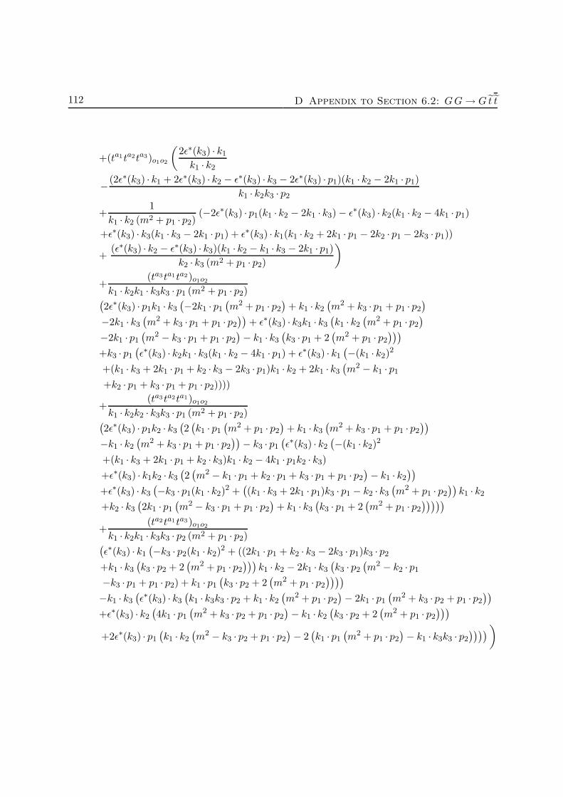
112 D Appendix to Section 6.2: GG→ G t t
+(ta1ta2ta3)o1o2
(2ε∗(k3) · k1
k1 · k2
−(2ε∗(k3) · k1 + 2ε∗(k3) · k2 − ε∗(k3) · k3 − 2ε∗(k3) · p1)(k1 · k2 − 2k1 · p1)
k1 · k2k3 · p2
+1
k1 · k2 (m2 + p1 · p2)(−2ε∗(k3) · p1(k1 · k2 − 2k1 · k3) − ε∗(k3) · k2(k1 · k2 − 4k1 · p1)
+ε∗(k3) · k3(k1 · k3 − 2k1 · p1) + ε∗(k3) · k1(k1 · k2 + 2k1 · p1 − 2k2 · p1 − 2k3 · p1))
+(ε∗(k3) · k2 − ε∗(k3) · k3)(k1 · k2 − k1 · k3 − 2k1 · p1)
k2 · k3 (m2 + p1 · p2)
)
+(ta3 ta1ta2)o1o2
k1 · k2k1 · k3k3 · p1 (m2 + p1 · p2)(2ε∗(k3) · p1k1 · k3
(−2k1 · p1
(m2 + p1 · p2
)+ k1 · k2
(m2 + k3 · p1 + p1 · p2
)
−2k1 · k3
(m2 + k3 · p1 + p1 · p2
))+ ε∗(k3) · k3k1 · k3
(k1 · k2
(m2 + p1 · p2
)
−2k1 · p1
(m2 − k3 · p1 + p1 · p2
)− k1 · k3
(k3 · p1 + 2
(m2 + p1 · p2
)))
+k3 · p1
(ε∗(k3) · k2k1 · k3(k1 · k2 − 4k1 · p1) + ε∗(k3) · k1
(−(k1 · k2)
2
+(k1 · k3 + 2k1 · p1 + k2 · k3 − 2k3 · p1)k1 · k2 + 2k1 · k3
(m2 − k1 · p1
+k2 · p1 + k3 · p1 + p1 · p2))))
+(ta3 ta2ta1)o1o2
k1 · k2k2 · k3k3 · p1 (m2 + p1 · p2)(2ε∗(k3) · p1k2 · k3
(2(k1 · p1
(m2 + p1 · p2
)+ k1 · k3
(m2 + k3 · p1 + p1 · p2
))
−k1 · k2
(m2 + k3 · p1 + p1 · p2
))− k3 · p1
(ε∗(k3) · k2
(−(k1 · k2)
2
+(k1 · k3 + 2k1 · p1 + k2 · k3)k1 · k2 − 4k1 · p1k2 · k3)
+ε∗(k3) · k1k2 · k3
(2(m2 − k1 · p1 + k2 · p1 + k3 · p1 + p1 · p2
)− k1 · k2
))
+ε∗(k3) · k3
(−k3 · p1(k1 · k2)
2 +((k1 · k3 + 2k1 · p1)k3 · p1 − k2 · k3
(m2 + p1 · p2
))k1 · k2
+k2 · k3
(2k1 · p1
(m2 − k3 · p1 + p1 · p2
)+ k1 · k3
(k3 · p1 + 2
(m2 + p1 · p2
)))))
+(ta2 ta1ta3)o1o2
k1 · k2k1 · k3k3 · p2 (m2 + p1 · p2)(ε∗(k3) · k1
(−k3 · p2(k1 · k2)
2 + ((2k1 · p1 + k2 · k3 − 2k3 · p1)k3 · p2
+k1 · k3
(k3 · p2 + 2
(m2 + p1 · p2
)))k1 · k2 − 2k1 · k3
(k3 · p2
(m2 − k2 · p1
−k3 · p1 + p1 · p2) + k1 · p1
(k3 · p2 + 2
(m2 + p1 · p2
))))
−k1 · k3
(ε∗(k3) · k3
(k1 · k3k3 · p2 + k1 · k2
(m2 + p1 · p2
)− 2k1 · p1
(m2 + k3 · p2 + p1 · p2
))
+ε∗(k3) · k2
(4k1 · p1
(m2 + k3 · p2 + p1 · p2
)− k1 · k2
(k3 · p2 + 2
(m2 + p1 · p2
)))
+2ε∗(k3) · p1
(k1 · k2
(m2 − k3 · p2 + p1 · p2
)− 2
(k1 · p1
(m2 + p1 · p2
)− k1 · k3k3 · p2
)))))
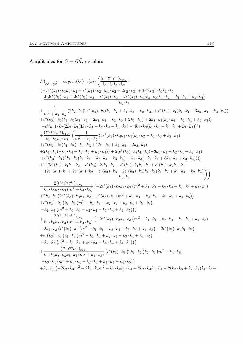
D.2 Feynman Amplitudes 113
Amplitudes for G→ Gtt, ε scalars
Mφφ→getet
= αsgsπε(k1) · ε(k2)
((ta1 ta2ta3)o1o2
k1 · k2k2 · k3×
(−2ε∗(k3) · k3k1 · k2 + ε∗(k3) · k2(4k1 · k2 − 2k2 · k3) + 2ε∗(k3) · k1k2 · k3
−2(2ε∗(k3) · k1 + 2ε∗(k3) · k2 − ε∗(k3) · k3 − 2ε∗(k3) · k4)k2 · k3(k1 · k2 − k1 · k4 + k2 · k4)
k3 · k5
+1
m2 + k4 · k5(2k2 · k3(2ε
∗(k3) · k4(k1 · k2 + k1 · k3 − k2 · k3) + ε∗(k3) · k1(k1 · k4 − 3k2 · k4 − k3 · k4))
+ε∗(k3) · k3(k2 · k3(k1 · k3 − 2k1 · k4 − k2 · k3 + 2k2 · k4) + 2k1 · k2(k1 · k4 − k2 · k4 + k3 · k4))
+ε∗(k3) · k2(2k2 · k3(3k1 · k4 − k2 · k4 + k3 · k4) − 4k1 · k2(k1 · k4 − k2 · k4 + k3 · k4))))
+(ta2ta1ta3)o1o2
k1 · k2k1 · k3
(1
m2 + k4 · k5(4ε∗(k3) · k4k1 · k3(k1 · k2 − k1 · k3 + k2 · k3)
+ε∗(k3) · k3(k1 · k3(−k1 · k3 + 2k1 · k4 + k2 · k3 − 2k2 · k4)
+2k1 · k2(−k1 · k4 + k2 · k4 + k3 · k4)) + 2(ε∗(k3) · k2k1 · k3(−3k1 · k4 + k2 · k4 − k3 · k4)
+ε∗(k3) · k1(2k1 · k2(k1 · k4 − k2 · k4 − k3 · k4) + k1 · k3(−k1 · k4 + 3k2 · k4 + k3 · k4))))
+2 (2ε∗(k3) · k1k1 · k2 − ε∗(k3) · k3k1 · k2 − ε∗(k3) · k1k1 · k3 + ε∗(k3) · k2k1 · k3
−(2ε∗(k3) · k1 + 2ε∗(k3) · k2 − ε∗(k3) · k3 − 2ε∗(k3) · k4)k1 · k3(k1 · k2 + k1 · k4 − k2 · k4)
k3 · k5
))
− 2(ta2 ta3ta1)o1o2
k1 · k3k2 · k3 (m2 + k4 · k5)
(−2ε∗(k3) · k2k1 · k3
(m2 + k1 · k4 − k2 · k4 + k3 · k4 + k4 · k5
)
+2k2 · k3
(2ε∗(k3) · k4k1 · k3 + ε∗(k3) · k1
(m2 + k1 · k4 − k2 · k4 − k3 · k4 + k4 · k5
))
+ε∗(k3) · k3
(k1 · k3
(m2 + k1 · k4 − k2 · k4 + k3 · k4 + k4 · k5
)
−k2 · k3
(m2 + k1 · k4 − k2 · k4 − k3 · k4 + k4 · k5
)))
+2(ta1 ta3ta2)o1o2
k1 · k3k2 · k3 (m2 + k4 · k5)
(−2ε∗(k3) · k2k1 · k3
(m2 − k1 · k4 + k2 · k4 − k3 · k4 + k4 · k5
)
+2k2 · k3
(ε∗(k3) · k1
(m2 − k1 · k4 + k2 · k4 + k3 · k4 + k4 · k5
)− 2ε∗(k3) · k4k1 · k3
)
+ε∗(k3) · k3
(k1 · k3
(m2 − k1 · k4 + k2 · k4 − k3 · k4 + k4 · k5
)
−k2 · k3
(m2 − k1 · k4 + k2 · k4 + k3 · k4 + k4 · k5
)))
+(ta3ta2 ta1)o1o2
k1 · k2k2 · k3k3 · k4 (m2 + k4 · k5)
(ε∗(k3) · k3
(2k1 · k2
(k2 · k3
(m2 + k4 · k5
)
+k3 · k4
(m2 + k1 · k4 − k2 · k4 + k3 · k4 + k4 · k5
))
+k2 · k3
(−2k2 · k3m
2 − 2k2 · k4m2 − k2 · k3k3 · k4 + 2k2 · k4k3 · k4 − 2(k2 · k3 + k2 · k4)k4 · k5+

114 D Appendix to Section 6.2: GG→ G t t
+2k1 · k4
(m2 − k3 · k4 + k4 · k5
)+ k1 · k3
(k3 · k4 + 2
(m2 + k4 · k5
))))
−2(k3 · k4
(ε∗(k3) · k1k2 · k3
(m2 − k1 · k4 + 3k2 · k4 + k3 · k4 + k4 · k5
)
+ε∗(k3) · k2
(2k1 · k2
(m2 + k1 · k4 − k2 · k4 + k3 · k4 + k4 · k5
)
−k2 · k3
(m2 + 3k1 · k4 − k2 · k4 + k3 · k4 + k4 · k5
)))− 2ε∗(k3) · k4k2 · k3
(k1 · k4m
2
−k2 · k3m2 − k2 · k4m
2 − k2 · k3k3 · k4 + (k1 · k4 − k2 · k3 − k2 · k4)k4 · k5 +
k1 · k2
(m2 + k3 · k4 + k4 · k5
)+ k1 · k3
(m2 + k3 · k4 + k4 · k5
))))
+(ta3ta1ta2)o1o2
k1 · k2k1 · k3k3 · k4 (m2 + k4 · k5)
(ε∗(k3) · k3
(2k1 · k2
(k1 · k3
(m2 + k4 · k5
)
+k3 · k4
(m2 − k1 · k4 + k2 · k4 + k3 · k4 + k4 · k5
))+ k1 · k(k3)
(2k2 · k3m
2 + 2k2 · k4m2
+k2 · k3k3 · k4 − 2k2 · k4k3 · k4 + 2(k2 · k3 + k2 · k4)k4 · k5 − 2k1 · k4
(m2 − k3 · k4 + k4 · k5
)
−k1 · k3
(k3 · k4 + 2
(m2 + k4 · k5
))))− 2
(k3 · k4
(ε∗(k3) · k2k1 · k3
(m2 + 3k1 · k4 − k2 · k4
+k3 · k4 + k4 · k5) + ε∗(k3) · k1
(2k1 · k2
(m2 − k1 · k4 + k2 · k4 + k3 · k4 + k4 · k5
)
−k1 · k3
(m2 − k1 · k4 + 3k2 · k4 + k3 · k4 + k4 · k5
)))
−2ε∗(k3) · k4k1 · k3
(−k1 · k4m
2 + k2 · k3m2 + k2 · k4m
2 + k2 · k3k3 · k4
−(k1 · k4 − k2 · k3 − k2 · k4)k4 · k5 + k1 · k2
(m2 + k3 · k4 + k4 · k5
)
−k1 · k3
(m2 + k3 · k4 + k4 · k5
)))))
Mgφ→φetet
=αsgsπε(k2) · ε∗(k3)
k1 · k2k1 · k3k1 · k4k1 · k5k2 · k3 (m2 + k4 · k5)×
((ta1ta2ta3)o1o2k1 · k3k1 · k5
(ε(k1) · k1
((k1 · k4 − 2
(m2 + k4 · k5
))(k1 · k2)
2
+(k1 · k3
(k1 · k4 − 2
(m2 + k4 · k5
))+ 2
(k2 · k3
(m2 + k4 · k5
)
+(k2 · k4 + k3 · k4)(m2 + k1 · k4 + k4 · k5
)))k1 · k2 − 2k1 · k4k2 · k3
(−m2
+k1 · k4 + k2 · k4 + k3 · k4 − k4 · k5))
+2(2ε(k1) · k4k1 · k2
(−k2 · k3m
2 − k2 · k4m2 − k3 · k4m
2 + k1 · k4k2 · k3
−(k2 · k3 + k2 · k4 + k3 · k4)k4 · k5 + k1 · k2
(m2 − k1 · k4 + k4 · k5
)
+k1 · k3
(m2 − k1 · k4 + k4 · k5
))+ k1 · k4
(ε(k1) · k2
(k1 · k2
(−m2 + k1 · k4 + k2 · k4
+3k3 · k4 − k4 · k5) + 2k2 · k3
(m2 − k1 · k4 − k2 · k4 − k3 · k4 + k4 · k5
))
−ε(k1) · k3k1 · k2
(m2 − k1 · k4 + 3k2 · k4 + k3 · k4 + k4 · k5
))))
+(ta1ta3ta2)o1o2k1 · k2k1 · k5
(ε(k1) · k1
((2(m2 + k4 · k5
)− k1 · k4
)(k1 · k3)
2
+k1 · k2
(2(m2 + k4 · k5
)− k1 · k4
)k1 · k3 + 2
(k2 · k3
(m2 + k4 · k5
)
−(k2 · k4 + k3 · k4)(m2 + k1 · k4 + k4 · k5
))k1 · k3
+2k1 · k4k2 · k3
(−m2 + k1 · k4 − k2 · k4 − k3 · k4 − k4 · k5
))
+2(2ε(k1) · k4k1 · k3
(−k2 · k3m
2 + k2 · k4m2 + k3 · k4m
2 + k1 · k4k2 · k3
−(k2 · k3 − k2 · k4 − k3 · k4)k4 · k5 − k1 · k2
(m2 − k1 · k4 + k4 · k5
)
−k1 · k3
(m2 − k1 · k4 + k4 · k5
))+ k1 · k4
(ε(k1) · k2k1 · k3
(m2 − k1 · k4−
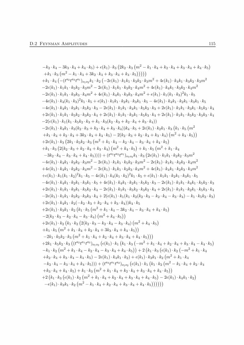
D.2 Feynman Amplitudes 115
−k2 · k4 − 3k3 · k4 + k4 · k5) + ε(k1) · k3
(2k2 · k3
(m2 − k1 · k4 + k2 · k4 + k3 · k4 + k4 · k5
)
+k1 · k3
(m2 − k1 · k4 + 3k2 · k4 + k3 · k4 + k4 · k5
)))))
+k1 · k4
(−(ta2ta3ta1)o1o2k1 · k2
(−2ε(k1) · k1k1 · k3k2 · k3m
2 + 4ε(k1) · k4k1 · k3k2 · k3m2
−2ε(k1) · k1k1 · k5k2 · k3m2 − 2ε(k1) · k1k1 · k3k2 · k4m
2 + 4ε(k1) · k4k1 · k3k2 · k4m2
−2ε(k1) · k1k1 · k3k3 · k4m2 + 4ε(k1) · k4k1 · k3k3 · k4m
2 + ε(k1) · k1(k1 · k3)2k1 · k5
−4ε(k1) · k4(k1 · k3)2k1 · k5 + ε(k1) · k1k1 · k2k1 · k3k1 · k5 − 4ε(k1) · k4k1 · k2k1 · k3k1 · k5
−4ε(k1) · k4k1 · k3k1 · k5k2 · k3 − 2ε(k1) · k1k1 · k4k1 · k5k2 · k3 + 2ε(k1) · k1k1 · k3k1 · k5k2 · k4
+2ε(k1) · k1k1 · k5k2 · k3k2 · k4 + 2ε(k1) · k1k1 · k3k1 · k5k3 · k4 + 2ε(k1) · k1k1 · k5k2 · k3k3 · k4
−2(ε(k1) · k1(k1 · k5k2 · k3 + k1 · k3(k2 · k3 + k2 · k4 + k3 · k4))
−2ε(k1) · k4k1 · k3(k2 · k3 + k2 · k4 + k3 · k4))k4 · k5 + 2ε(k1) · k2k1 · k3
(k1 · k5
(m2
+k1 · k4 + k2 · k4 + 3k3 · k4 + k4 · k5) − 2(k2 · k3 + k2 · k4 + k3 · k4)(m2 + k4 · k5
))
+2ε(k1) · k3
(2k1 · k5k2 · k3
(m2 + k1 · k4 − k2 · k4 − k3 · k4 + k4 · k5
)
+k1 · k3
(2(k2 · k3 + k2 · k4 + k3 · k4)
(m2 + k4 · k5
)+ k1 · k5
(m2 + k1 · k4
−3k2 · k4 − k3 · k4 + k4 · k5)))) + (ta3 ta2ta1)o1o2k1 · k3
(2ε(k1) · k1k1 · k2k2 · k3m
2
−4ε(k1) · k4k1 · k2k2 · k3m2 − 2ε(k1) · k1k1 · k5k2 · k3m
2 − 2ε(k1) · k1k1 · k2k2 · k4m2
+4ε(k1) · k4k1 · k2k2 · k4m2 − 2ε(k1) · k1k1 · k2k3 · k4m
2 + 4ε(k1) · k4k1 · k2k3 · k4m2
+ε(k1) · k1(k1 · k2)2k1 · k5 − 4ε(k1) · k4(k1 · k2)
2k1 · k5 + ε(k1) · k1k1 · k2k1 · k3k1 · k5
−4ε(k1) · k4k1 · k2k1 · k3k1 · k5 + 4ε(k1) · k4k1 · k2k1 · k5k2 · k3 − 2ε(k1) · k1k1 · k4k1 · k5k2 · k3
+2ε(k1) · k1k1 · k2k1 · k5k2 · k4 − 2ε(k1) · k1k1 · k5k2 · k3k2 · k4 + 2ε(k1) · k1k1 · k2k1 · k5k3 · k4
−2ε(k1) · k1k1 · k5k2 · k3k3 · k4 + 2(ε(k1) · k1(k1 · k2(k2 · k3 − k2 · k4 − k3 · k4) − k1 · k5k2 · k3)
+2ε(k1) · k4k1 · k2(−k2 · k3 + k2 · k4 + k3 · k4))k4 · k5
+2ε(k1) · k3k1 · k2
(k1 · k5
(m2 + k1 · k4 − 3k2 · k4 − k3 · k4 + k4 · k5
)
−2(k2 · k3 − k2 · k4 − k3 · k4)(m2 + k4 · k5
))
+2ε(k1) · k2
(k1 · k2
(2(k2 · k3 − k2 · k4 − k3 · k4)
(m2 + k4 · k5
)
+k1 · k5
(m2 + k1 · k4 + k2 · k4 + 3k3 · k4 + k4 · k5
))
−2k1 · k5k2 · k3
(m2 + k1 · k4 + k2 · k4 + k3 · k4 + k4 · k5
)))
+2k1 · k5k2 · k3
((ta2ta1ta3)o1o2
(ε(k1) · k1
(k1 · k3
(−m2 + k1 · k4 + k2 · k4 + k3 · k4 − k4 · k5
)
−k1 · k2
(m2 + k1 · k4 − k2 · k4 − k3 · k4 + k4 · k5
))+ 2
(k1 · k3
(ε(k1) · k2
(−m2 + k1 · k4
+k2 · k4 + k3 · k4 − k4 · k5) − 2ε(k1) · k4k1 · k2) + ε(k1) · k3k1 · k2
(m2 + k1 · k4
−k2 · k4 − k3 · k4 + k4 · k5))) + (ta3ta1ta2)o1o2
(ε(k1) · k1
(k1 · k2
(m2 − k1 · k4 + k2 · k4
+k3 · k4 + k4 · k5) + k1 · k3
(m2 + k1 · k4 + k2 · k4 + k3 · k4 + k4 · k5
))
+2(k1 · k3
(ε(k1) · k2
(m2 + k1 · k4 + k2 · k4 + k3 · k4 + k4 · k5
)− 2ε(k1) · k4k1 · k2
)
−ε(k1) · k3k1 · k2
(m2 − k1 · k4 + k2 · k4 + k3 · k4 + k4 · k5
))))))

116 D Appendix to Section 6.2: GG→ G t t
Mφg→φetet
=αsgsπε(k1) · ε∗(k3)
k1 · k2k1 · k3k2 · k3k2 · k4k2 · k5 (m2 + k4 · k5)×
((ta3ta1ta2)o1o2k2 · k3k2 · k4
(ε(k2) · k2
(k2 · k5(k1 · k2)
2 +(−2k3 · k4m
2 + k2 · k5(k2 · k3 + 2k3 · k4)
−2k3 · k4k4 · k5 + 2k1 · k3
(m2 + k4 · k5
)− 2k1 · k4
(m2 − k2 · k5 + k4 · k5
))k1 · k2
−2k1 · k3k2 · k5
(m2 + k1 · k4 + k2 · k4 + k3 · k4 + k4 · k5
))
+2ε(k2) · k1
(k1 · k2
(k2 · k5m
2 − 2k3 · k4m2 + k2 · k4k2 · k5 + 3k2 · k5k3 · k4
+(k2 · k5 − 2k3 · k4)k4 · k5 + 2k1 · k3
(m2 + k4 · k5
)+ k1 · k4
(k2 · k5 − 2
(m2 + k4 · k5
)))
−2k1 · k3k2 · k5
(m2 + k1 · k4 + k2 · k4 + k3 · k4 + k4 · k5
))
+2k1 · k2
(2ε(k2) · k4
(−(k1 · k2 + k2 · k3)k2 · k5 + (k1 · k4 + k3 · k4)
(m2 + k4 · k5
)
−k1 · k3
(m2 − k2 · k5 + k4 · k5
))+ ε(k2) · k3
(k2 · k5m
2 + 2k3 · k4m2 + k2 · k4k2 · k5
−k2 · k5k3 · k4 + (k2 · k5 + 2k3 · k4)k4 · k5 − 2k1 · k3
(m2 + k4 · k5
)
+k1 · k4
(2(m2 + k4 · k5
)− 3k2 · k5
))))
−(ta1ta3ta2)o1o2k1 · k2k2 · k4
(2ε(k2) · k1k2 · k3
(k2 · k5m
2 − 2k3 · k4m2
+k2 · k4k2 · k5 + 3k2 · k5k3 · k4 + (k2 · k5 − 2k3 · k4)k4 · k5 − 2k1 · k3
(m2 + k4 · k5
)
+k1 · k4
(k2 · k5 − 2
(m2 + k4 · k5
)))+ ε(k2) · k2 (k2 · k3 (k1 · k2k2 · k5
+k2 · k3k2 · k5 − 2k1 · k4
(m2 − k2 · k5 + k4 · k5
)− 2k3 · k4
(m2 − k2 · k5 + k4 · k5
))
−2k1 · k3
(k2 · k3
(m2 + k4 · k5
)+ k2 · k5
(m2 − k1 · k4 + k2 · k4 − k3 · k4 + k4 · k5
)))
+2(2ε(k2) · k4k2 · k3
(−(k1 · k2 + k2 · k3)k2 · k5 + (k1 · k4 + k3 · k4)
(m2 + k4 · k5
)
+k1 · k3
(m2 − k2 · k5 + k4 · k5
))+ ε(k2) · k3
(2k1 · k3
(k2 · k3
(m2 + k4 · k5
)
+k2 · k5
(m2 − k1 · k4 + k2 · k4 − k3 · k4 + k4 · k5
))+ k2 · k3
(2k3 · k4
(m2 + k4 · k5
)
+k2 · k5
(m2 + k2 · k4 − k3 · k4 + k4 · k5
)+ k1 · k4
(2(m2 + k4 · k5
)− 3k2 · k5
)))))
+k2 · k5
((ta2 ta1ta3)o1o2k2 · k3
(ε(k2) · k2
((k2 · k4 − 2
(m2 + k4 · k5
))(k1 · k2)
2
+(−2k2 · k3m
2 + 2k3 · k4m2 + k2 · k3k2 · k4 + 2k2 · k4k3 · k4 − 2(k2 · k3 − k3 · k4)k4 · k5
+2k1 · k3
(m2 + k4 · k5
)+ 2k1 · k4
(m2 + k2 · k4 + k4 · k5
))k1 · k2
−2k1 · k3k2 · k4
(−m2 + k1 · k4 + k2 · k4 + k3 · k4 − k4 · k5
))
−2(2ε(k2) · k4k1 · k2
(k1 · k4m
2f − k2 · k3m2 + k3 · k4m
2 + k2 · k3k2 · k4
+(k1 · k4 − k2 · k3 + k3 · k4)k4 · k5 − k1 · k2
(m2 − k2 · k4 + k4 · k5
)
+k1 · k3
(m2 − k2 · k4 + k4 · k5
))+ k2 · k4
(ε(k2) · k3k1 · k2
(m2 + 3k1 · k4 − k2 · k4
+k3 · k4 + k4 · k5) + ε(k2) · k1
(2k1 · k3
(−m2 + k1 · k4 + k2 · k4 + k3 · k4 − k4 · k5
)
+k1 · k2
(m2 − k1 · k4 − k2 · k4 − 3k3 · k4 + k4 · k5 ))
)))
+(ta2ta3ta1)o1o2k1 · k2
(ε(k2) · k2
(k1 · k2k2 · k3
(2(m2 + k4 · k5
)− k2 · k4
)
+2k1 · k3
(k2 · k4
(−m2 − k1 · k4 + k2 · k4 − k3 · k4 − k4 · k5
)+ k2 · k3
(m2 + k4 · k5
))
+k2 · k3
(−2k1 · k4
(m2 + k2 · k4 + k4 · k5
)− 2k3 · k4
(m2 + k2 · k4 + k4 · k5
)
+k2 · k3
(2(m2 + k4 · k5
)− k2 · k4
)))+ 2
(2ε(k2) · k4k2 · k3
(k1 · k4m
2 − k2 · k3m2
+k3 · k4m2 + k2 · k3k2 · k4 + (k1 · k4 − k2 · k3 + k3 · k4)k4 · k5
−k1 · k2
(m2 − k2 · k4 + k4 · k5
)− k1 · k3
(m2 − k2 · k4 + k4 · k5
))
+k2 · k4
(ε(k2) · k1k2 · k3
(m2 − k1 · k4 − k2 · k4 − 3k3 · k4 + k4 · k5
)+

D.2 Feynman Amplitudes 117
+ε(k2) · k3
(2k1 · k3
(m2 + k1 · k4 − k2 · k4 + k3 · k4 + k4 · k5
)
+k2 · k3
(m2 + 3k1 · k4 − k2 · k4 + k3 · k4 + k4 · k5
)))))
+2k1 · k3k2 · k4
((ta1ta2ta3)o1o2
(ε(k2) · k2
(k2 · k3
(−m2 + k1 · k4 + k2 · k4 + k3 · k4 − k4 · k5
)
−k1 · k2
(m2 − k1 · k4 + k2 · k4 − k3 · k4 + k4 · k5
))+ 2
(k2 · k3
(ε(k2) · k1
(−m2 + k1 · k4
+k2 · k4 + k3 · k4 − k4 · k5) − 2ε(k2) · k4k1 · k2) + ε(k2) · k3k1 · k2
(m2 − k1 · k4 + k2 · k4
−k3 · k4 + k4 · k5)))
+(ta3 ta2ta1)o1o2
(ε(k2) · k2
(k1 · k2
(m2 + k1 · k4
−k2 · k4 + k3 · k4 + k4 · k5) + k2 · k3
(m2 + k1 · k4 + k2 · k4 + k3 · k4 + k4 · k5
))
+2(k2 · k3
(ε(k2) · k1
(m2 + k1 · k4 + k2 · k4 + k3 · k4 + k4 · k5
)− 2ε(k2) · k4k1 · k2
)
−ε(k2) · k3k1 · k2
(m2 + k1 · k4 − k2 · k4 + k3 · k4 + k4 · k5
))))))

118 D Appendix to Section 6.2: GG→ G t t
D.3 Squared Amplitudes
Squared Amplitudes for GG → Gtt, ε Scalars
|M|2φ g→φet et
=1024αsα
2s(D − 4)π3
9st1u21(s+ t1 + u1)2u2
6(s+ t1 + u6)2(144m2st71 + 576m2s2t61 + 81u1u
26t
61
+288m2ss4t61 + 432m2su1t
61 − 9u2
1u6t61 + 612m2su6t
61 − 9su1u6t
61 + 81s4u1u6t
61
+864m2s3t51 + 243u1u36t
51 + 144m2ss24t
51 + 496m2su2
1t51 + 126u2
1u26t
51 + 1116m2su2
6t51
+225su1u26t
51 + 567s4u1u
26t
51 + 1152m2s2s4t
51 + 1440m2s2u1t
51 + 720m2ss4u1t
51
−27u31u6t
51 + 1836m2s2u6t
51 − 71su2
1u6t51 + 153s4u
21u6t
51 + 936m2ss4u6t
51 − 36s2u1u6t
51
+162s24u1u6t51 + 1530m2su1u6t
51 + 216ss4u1u6t
51 + 576m2s4t41 + 243u1u
46t
41
+272m2su31t
41 + 360u2
1u36t
41 + 972m2su3
6t41 + 558su1u
36t
41 + 1053s4u1u
36t
41 − 167s2u2
1u6t41
+576m2s2s24t41 + 1408m2s2u2
1t41 + 576m2ss4u
21t
41 − 90u3
1u26t
41 + 2232m2s2u2
6t41
+64su21u
26t
41 + 864s4u
21u
26t
41 + 1296m2ss4u
26t
41 + 189s2u1u
26t
41 + 729s24u1u
26t
41 + 288m2ss24u1t
41
+2232m2su1u26t
41 + 1332ss4u1u
26t
41 + 1728m2s3s4t
41 + 1728m2s3u1t
41
+2304m2s2s4u1t41 − 27u4
1u6t41 + 1836m2s3u6t
41 − 132su3
1u6t41 + 63s4u
31u6t
41 + 324m2ss24u6t
41
+243s24u21u6t
41 + 1512m2su2
1u6t41 + 144ss4u
21u6t
41 + 2808m2s2s4u6t
41 − 54s3u1u6t
41
+3690m2s2u1u6t41 + 387ss24u1u6t
41 + 72s2s4u1u6t
41 + 2034m2ss4u1u6t
41 + 144m2s5t31
+81u1u56t
31 + 64m2su4
1t31 + 306u2
1u46t
31 + 324m2su4
6t31 + 405su1u
46t
31 + 81s34u1u6t
41
+729s4u1u46t
31 + 672m2s2u3
1t31 + 144m2ss4u
31t
31 − 180u3
1u36t
31 + 972m2s2u3
6t31
+261su21u
36t
31 + 1197s4u
21u
36t
31 + 648m2ss4u
36t
31 + 387s2u1u
36t
31 + 891s24u1u
36t
31
+1926ss4u1u36t
31 + 864m2s3s24t
31 + 1392m2s3u2
1t31 + 144m2ss24u
21t
31 + 1440m2s2s4u
21t
31
−234u41u
26t
31 + 1116m2s3u2
6t31 − 681su3
1u26t
31 + 189s4u
31u
26t
31 + 324m2ss24u
26t
31 − 357s2u2
1u26t
31
+891s24u21u
26t
31 + 2052m2su2
1u26t
31 + 648ss4u
21u
26t
31 + 2592m2s2s4u
26t
31 + 27s3u1u
26t
31
+243s34u1u26t
31 + 3528m2s2u1u
26t
31 + 1278ss24u1u
26t
31 + 774s2s4u1u
26t
31 + 2430m2ss4u1u
26t
31
+1152m2s4s4t31 + 864m2s4u1t
31 + 864m2s2s24u1t
31 + 2592m2s3s4u1t
31 − 9u5
1u6t31
+612m2s4u6t31 − 87su4
1u6t31 − 9s4u
41u6t
31 − 207s2u3
1u6t31 + 81s24u
31u6t
31 + 1458m2su1u
36t
31
+720m2su31u6t
31 − 180ss4u
31u6t
31 + 972m2s2s24u6t
31 − 165s3u2
1u6t31 + 81s34u
21u6t
31
+3024m2s2u21u6t
31 + 288ss24u
21u6t
31 − 522s2s4u
21u6t
31 + 1422m2ss4u
21u6t
31 + 2808m2s3s4u6t
31
−36s4u1u6t31 + 2790m2s3u1u6t
31 + 162ss34u1u6t
31 + 108s2s24u1u6t
31 + 648m2ss24u1u6t
31
−270s3s4u1u6t31 + 4554m2s2s4u1u6t
31 + 81u2
1u56t
21 + 81su1u
56t
21 + 162s4u1u
56t
21
−198u31u
46t
21 + 126su2
1u46t
21 + 486s4u
21u
46t
21 + 162s2u1u
46t
21 + 324s24u1u
46t
21 + 324m2su1u
46t
21
+972ss4u1u46t
21 + 528m2s3u3
1t21 + 288m2s2s4u
31t
21 − 468u4
1u36t
21 − 1071su3
1u36t
21
−297s2u21u
36t
21 + 810s24u
21u
36t
21 + 1296m2su2
1u36t
21 + 27ss4u
21u
36t
21 + 648m2s2s4u
36t
21
+72s3u1u36t
21 − 117s4u
31u
36t
21 + 128m2s2u4
1t21 + +162s34u1u
36t
21 + 1134m2s2u1u
36t
21
D.3 Squared Amplitudes 119
+972ss24u1u36t
21 + 855s2s4u1u
36t
21 + 972m2ss4u1u
36t
21 + 576m2s4s24t
21 + 544m2s4u2
1t21
+288m2s2s24u21t
21 + 1152m2s3s4u
21t
21 − 99u5
1u26t
21 − 690su4
1u26t
21 − 108s4u
41u
26t
21
−1047s2u31u
26t
21 + 162s24u
31u
26t
21 + 738m2su3
1u26t
21 − 945ss4u
31u
26t
21 + 648m2s2s24u
26t
21
−402s3u21u
26t
21 + 243s34u
21u
26t
21 + 2682m2s2u2
1u26t
21 + 288ss24u
21u
26t
21 − 1395s2s4u
21u
26t
21
+1458m2ss4u21u
26t
21 + 1296m2s3s4u
26t
21 − 18s4u1u
26t
21 + 1296m2s3u1u
26t
21
+243ss34u1u26t
21 + 126s2s24u1u
26t
21 + 648m2ss24u1u
26t
21 − 180s3s4u1u
26t
21
+3240m2s2s4u1u26t
21 + 288m2s5s4t
21 + 144m2s5u1t
21 + 864m2s3s24u1t
21
+1152m2s4s4u1t21 − 17su5
1u6t21 − 84s2u4
1u6t21 + 126m2su4
1u6t21
−108ss4u41u6t
21 − 126s3u3
1u6t21 + 1134m2s2u3
1u6t21 − 18ss24u
31u6t
21
−675s2s4u31u6t
21 + 324m2ss4u
31u6t
21 + 972m2s3s24u6t
21 − 68s4u2
1u6t21 + 1800m2s3u2
1u6t21
+81ss34u21u6t
21 − 396s2s24u
21u6t
21 + 324m2ss24u
21u6t
21 − 936s3s4u
21u6t
21 + 2232m2s2s4u
21u6t
21
+936m2s4s4u6t21 − 9s5u1u6t
21 + 630m2s4u1u6t
21 − 378s3s24u1u6t
21
+1296m2s2s24u1u6t21 − 297s4s4u1u6t
21 + 3006m2s3s4u1u6t
21 − 81u3
1u56t1 + 162ss4u1u
56t1
+64m2s3u41t1 − 342u4
1u46t1 − 603su3
1u46t1 − 405s4u
31u
46t1 − 99s2u2
1u46t1
+162s24u21u
46t1 + 324m2su2
1u46t1 − 567ss4u
21u
46t1 + 162ss24u1u
46t1
+243s2s4u1u46t1 + 128m2s4u3
1t1 + 144m2s3s4u31t1 − 171u5
1u36t1
−927su41u
36t1 − 261s4u
41u
36t1 − 1035s2u3
1u36t1 − 81s24u
31u
36t1
+162m2su31u
36t1 − 1638ss4u
31u
36t1 − 198s3u2
1u36t1 + 162s34u
21u
36t1 + 810m2s2u2
1u36t1
−567ss24u21u
36t1 − 1638s2s4u
21u
36t1 + 324m2ss4u
21u
36t1 − 243s2s24u1u
36t1 − 18s3s4u1u
36t1
+324m2s2s4u1u36t1 + 144m2s5s24t1 + 64m2s5u2
1t1 + 144m2s3s24u21t1
+288m2s4s4u21t1 − 170su5
1u26t1 − 591s2u4
1u26t1 + 126m2su4
1u26t1 − 423ss4u
41u
26t1
−528s3u31u
26t1 + 576m2s2u3
1u26t1 − 423ss24u
31u
26t1
+324m2ss4u31u
26t1 + 324m2s3s24u
26t1 − 107s4u2
1u26t1 + 774m2s3u2
1u26t1 − 1710s2s4u
31u
26t1
−1413s2s24u21u
26t1 + 324m2ss24u
21u
26t1 − 1476s3s4u
21u
26t1 + 1134m2s2s4u
21u
26t1
−243s2s34u1u26t1 − 666s3s24u1u
26t1 + 648m2s2s24u1u
26t1 − 189s4s4u1u
26t1 + 810m2s3s4u1u
26t1
+288m2s4s24u1t1 + 144m2s5s4u1t1 − 8s2u51u6t1 − 24s3u4
1u6t1 + 126m2s2u41u6t1
−24s4u31u6t1 + 414m2s3u3
1u6t1 − 261s2s24u31u6t1 − 576s3s4u
31u6t1 − 171s2s4u
41u6t1
+324m2s2s4u31u6t1 + 324m2s4s24u6t1 − 8s5u2
1u6t1 + 288m2s4u21u6t1 − 81s2s34u
21u6t1
−684s3s24u21u6t1 + 324m2s2s24u
21u6t1 − 495s4s4u
21u6t1 + 810m2s3s4u
21u6t1−
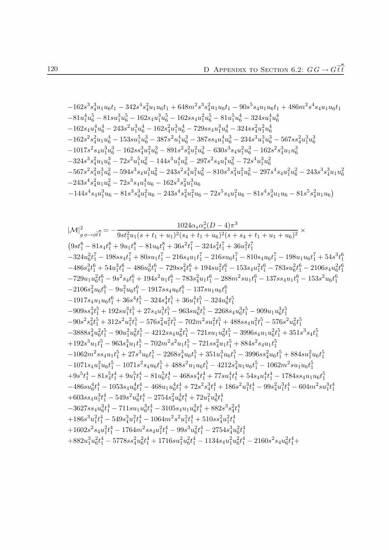
120 D Appendix to Section 6.2: GG→ G t t
−162s3s34u1u6t1 − 342s4s24u1u6t1 + 648m2s3s24u1u6t1 − 90s5s4u1u6t1 + 486m2s4s4u1u6t1
−81u41u
56 − 81su3
1u56 − 162s4u
31u
56 − 162ss4u
21u
56 − 81u5
1u46 − 324su4
1u46
−162s4u41u
46 − 243s2u3
1u46 − 162s24u
31u
46 − 729ss4u
31u
46 − 324ss24u
21u
46
−162s2s24u1u46 − 153su5
1u36 − 387s2u4
1u36 − 387ss4u
41u
36 − 234s3u3
1u36 − 567ss24u
31u
36
−1017s2s4u31u
36 − 162ss34u
21u
36 − 891s2s24u
21u
36 − 630s3s4u
21u
36 − 162s2s34u1u
36
−324s3s24u1u36 − 72s2u5
1u26 − 144s3u4
1u26 − 297s2s4u
41u
26 − 72s4u3
1u26
−567s2s24u31u
26 − 594s3s4u
31u
26 − 243s2s34u
21u
26 − 810s3s24u
21u
26 − 297s4s4u
21u
26 − 243s3s34u1u
26
−243s4s24u1u26 − 72s3s4u
41u6 − 162s3s24u
31u6
−144s4s4u31u6 − 81s3s34u
21u6 − 243s4s24u
21u6 − 72s5s4u
21u6 − 81s4s34u1u6 − 81s5s24u1u6
)
|M|2g φ→φet et
= − 1024αsα2s(D − 4)π3
9st21u1(s+ t1 + u1)2(s4 + t1 + u6)2(s+ s4 + t1 + u1 + u6)2×
(9st81 − 81s4t
81 + 9u1t
81 − 81u6t
81 + 36s2t71 − 324s24t
71 + 36u2
1t71
−324u26t
71 − 198ss4t
71 + 80su1t
71 − 216s4u1t
71 − 216su6t
71 − 810s4u6t
71 − 198u1u6t
71 + 54s3t61
−486s34t61 + 54u3
1t61 − 486u3
6t61 − 729ss24t
61 + 194su2
1t61 − 153s4u
21t
61 − 783su2
6t61 − 2106s4u
26t
61
−729u1u26t
61 − 9s2s4t
61 + 194s2u1t
61 − 783s24u1t
61 − 288m2su1t
61 − 137ss4u1t
61 − 153s2u6t
61
−2106s24u6t61 − 9u2
1u6t61 − 1917ss4u6t
61 − 137su1u6t
61
−1917s4u1u6t61 + 36s4t51 − 324s44t
51 + 36u4
1t51 − 324u4
6t51
−909ss34t51 + 192su3
1t51 + 27s4u
31t
51 − 963su3
6t51 − 2268s4u
36t
51 − 909u1u
36t
51
−90s2s24t51 + 312s2u2
1t51 − 576s24u
21t
51 − 702m2su2
1t51 + 488ss4u
21t
51 − 576s2u2
6t51
−3888s24u26t
51 − 90u2
1u26t
51 − 4212ss4u
26t
51 − 721su1u
26t
51 − 3996s4u1u
26t
51 + 351s3s4t
51
+192s3u1t51 − 963s34u1t
51 − 702m2s2u1t
51 − 721ss24u1t
51 + 884s2s4u1t
51
−1062m2ss4u1t51 + 27s3u6t
51 − 2268s34u6t
51 + 351u3
1u6t51 − 3996ss24u6t
51 + 884su2
1u6t51
−1071s4u21u6t
51 − 1071s2s4u6t
51 + 488s2u1u6t
51 − 4212s24u1u6t
51 − 1062m2su1u6t
51
+9s5t41 − 81s54t41 + 9u5
1t41 − 81u5
6t41 − 468ss44t
41 + 77su4
1t41 + 54s4u
41t
41 − 1784ss4u1u6t
51
−486su46t
41 − 1053s4u
46t
41 − 468u1u
46t
41 + 72s2s34t
41 + 186s2u3
1t41 − 99s24u
31t
41 − 604m2su3
1t41
+603ss4u31t
41 − 549s2u3
6t41 − 2754s24u
36t
41 + 72u2
1u36t
41
−3627ss4u36t
41 − 711su1u
36t
41 − 3105s4u1u
36t
41 + 882s3s24t
41
+186s3u21t
41 − 549s34u
21t
41 − 1064m2s2u2
1t41 + 510ss24u
21t
41
+1602s2s4u21t
41 − 1764m2ss4u
21t
41 − 99s3u2
6t41 − 2754s34u
26t
41
+882u31u
26t
41 − 5778ss24u
26t
41 + 1716su2
1u26t
41 − 1134s4u
21u
26t
41 − 2160s2s4u
26t
41+
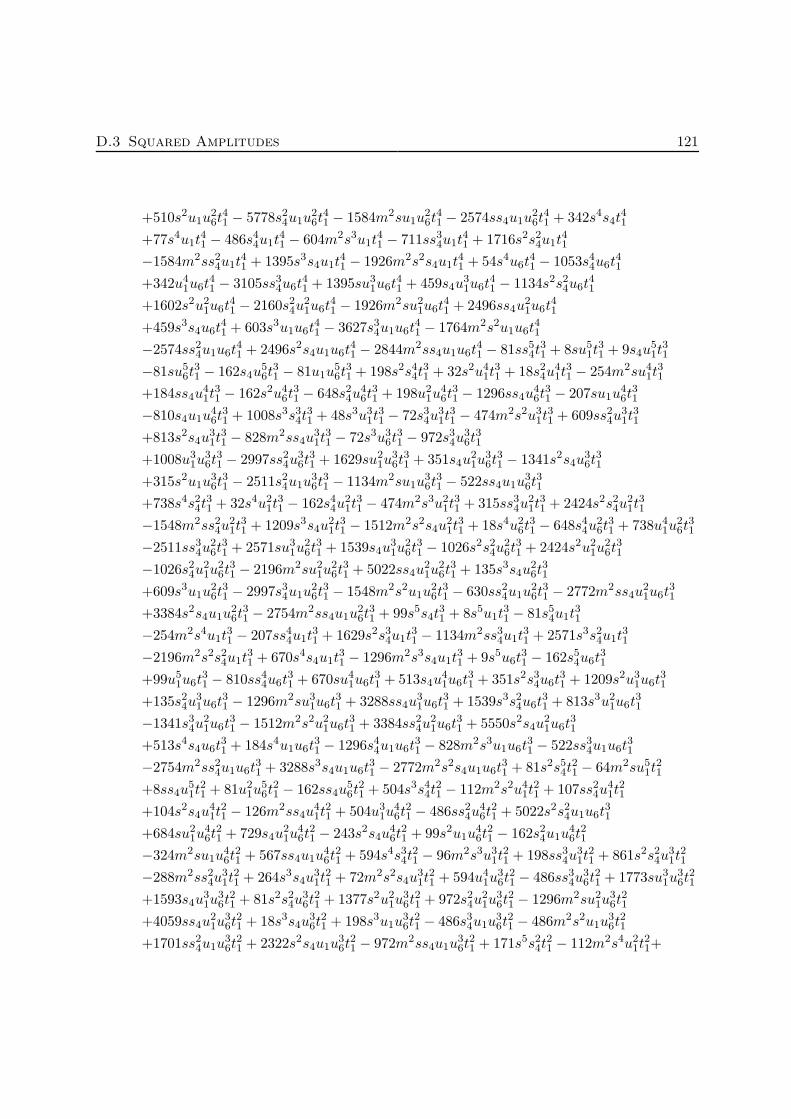
D.3 Squared Amplitudes 121
+510s2u1u26t
41 − 5778s24u1u
26t
41 − 1584m2su1u
26t
41 − 2574ss4u1u
26t
41 + 342s4s4t
41
+77s4u1t41 − 486s44u1t
41 − 604m2s3u1t
41 − 711ss34u1t
41 + 1716s2s24u1t
41
−1584m2ss24u1t41 + 1395s3s4u1t
41 − 1926m2s2s4u1t
41 + 54s4u6t
41 − 1053s44u6t
41
+342u41u6t
41 − 3105ss34u6t
41 + 1395su3
1u6t41 + 459s4u
31u6t
41 − 1134s2s24u6t
41
+1602s2u21u6t
41 − 2160s24u
21u6t
41 − 1926m2su2
1u6t41 + 2496ss4u
21u6t
41
+459s3s4u6t41 + 603s3u1u6t
41 − 3627s34u1u6t
41 − 1764m2s2u1u6t
41
−2574ss24u1u6t41 + 2496s2s4u1u6t
41 − 2844m2ss4u1u6t
41 − 81ss54t
31 + 8su5
1t31 + 9s4u
51t
31
−81su56t
31 − 162s4u
56t
31 − 81u1u
56t
31 + 198s2s44t
31 + 32s2u4
1t31 + 18s24u
41t
31 − 254m2su4
1t31
+184ss4u41t
31 − 162s2u4
6t31 − 648s24u
46t
31 + 198u2
1u46t
31 − 1296ss4u
46t
31 − 207su1u
46t
31
−810s4u1u46t
31 + 1008s3s34t
31 + 48s3u3
1t31 − 72s34u
31t
31 − 474m2s2u3
1t31 + 609ss24u
31t
31
+813s2s4u31t
31 − 828m2ss4u
31t
31 − 72s3u3
6t31 − 972s34u
36t
31
+1008u31u
36t
31 − 2997ss24u
36t
31 + 1629su2
1u36t
31 + 351s4u
21u
36t
31 − 1341s2s4u
36t
31
+315s2u1u36t
31 − 2511s24u1u
36t
31 − 1134m2su1u
36t
31 − 522ss4u1u
36t
31
+738s4s24t31 + 32s4u2
1t31 − 162s44u
21t
31 − 474m2s3u2
1t31 + 315ss34u
21t
31 + 2424s2s24u
21t
31
−1548m2ss24u21t
31 + 1209s3s4u
21t
31 − 1512m2s2s4u
21t
31 + 18s4u2
6t31 − 648s44u
26t
31 + 738u4
1u26t
31
−2511ss34u26t
31 + 2571su3
1u26t
31 + 1539s4u
31u
26t
31 − 1026s2s24u
26t
31 + 2424s2u2
1u26t
31
−1026s24u21u
26t
31 − 2196m2su2
1u26t
31 + 5022ss4u
21u
26t
31 + 135s3s4u
26t
31
+609s3u1u26t
31 − 2997s34u1u
26t
31 − 1548m2s2u1u
26t
31 − 630ss24u1u
26t
31 − 2772m2ss4u
21u6t
31
+3384s2s4u1u26t
31 − 2754m2ss4u1u
26t
31 + 99s5s4t
31 + 8s5u1t
31 − 81s54u1t
31
−254m2s4u1t31 − 207ss44u1t
31 + 1629s2s34u1t
31 − 1134m2ss34u1t
31 + 2571s3s24u1t
31
−2196m2s2s24u1t31 + 670s4s4u1t
31 − 1296m2s3s4u1t
31 + 9s5u6t
31 − 162s54u6t
31
+99u51u6t
31 − 810ss44u6t
31 + 670su4
1u6t31 + 513s4u
41u6t
31 + 351s2s34u6t
31 + 1209s2u3
1u6t31
+135s24u31u6t
31 − 1296m2su3
1u6t31 + 3288ss4u
31u6t
31 + 1539s3s24u6t
31 + 813s3u2
1u6t31
−1341s34u21u6t
31 − 1512m2s2u2
1u6t31 + 3384ss24u
21u6t
31 + 5550s2s4u
21u6t
31
+513s4s4u6t31 + 184s4u1u6t
31 − 1296s44u1u6t
31 − 828m2s3u1u6t
31 − 522ss34u1u6t
31
−2754m2ss24u1u6t31 + 3288s3s4u1u6t
31 − 2772m2s2s4u1u6t
31 + 81s2s54t
21 − 64m2su5
1t21
+8ss4u51t
21 + 81u2
1u56t
21 − 162ss4u
56t
21 + 504s3s44t
21 − 112m2s2u4
1t21 + 107ss24u
41t
21
+104s2s4u41t
21 − 126m2ss4u
41t
21 + 504u3
1u46t
21 − 486ss24u
46t
21 + 5022s2s24u1u6t
31
+684su21u
46t
21 + 729s4u
21u
46t
21 − 243s2s4u
46t
21 + 99s2u1u
46t
21 − 162s24u1u
46t
21
−324m2su1u46t
21 + 567ss4u1u
46t
21 + 594s4s34t
21 − 96m2s3u3
1t21 + 198ss34u
31t
21 + 861s2s24u
31t
21
−288m2ss24u31t
21 + 264s3s4u
31t
21 + 72m2s2s4u
31t
21 + 594u4
1u36t
21 − 486ss34u
36t
21 + 1773su3
1u36t
21
+1593s4u31u
36t
21 + 81s2s24u
36t
21 + 1377s2u2
1u36t
21 + 972s24u
21u
36t
21 − 1296m2su2
1u36t
21
+4059ss4u21u
36t
21 + 18s3s4u
36t
21 + 198s3u1u
36t
21 − 486s34u1u
36t
21 − 486m2s2u1u
36t
21
+1701ss24u1u36t
21 + 2322s2s4u1u
36t
21 − 972m2ss4u1u
36t
21 + 171s5s24t
21 − 112m2s4u2
1t21+

122 D Appendix to Section 6.2: GG→ G t t
+99ss44u21t
21 + 1377s2s34u
21t
21 − 486m2ss34u
21t
21 + 1572s3s24u
21t
21 − 738m2s2s24u
21t
21
+248s4s4u21t
21 − 378m2s3s4u
21t
21 + 171u5
1u26t
21 − 162ss44u
26t
21 + 989su4
1u26t
21
+864s4u41u
26t
21 + 972s2s34u
26t
21 + 1572s2u3
1u26t
21 + 1107s24u
31u
26t
21 − 1566m2su3
1u26t
21
+4239ss4u31u
26t
21 + 1107s3s24u
26t
21 + 861s3u2
1u26t
21 + 81s34u
21u
26t
21 − 738m2s2u2
1u26t
21
+5598ss24u21u
26t
21 + 5688s2s4u
21u
26t
21 − 1458m2ss4u
21u
26t
21 + 189s4s4u
26t
21 + 107s4u1u
26t
21
−486s44u1u26t
21 − 288m2s3u1u
26t
21 + 1701ss34u1u
26t
21 + 5598s2s24u1u
26t
21
−1296m2ss24u1u26t
21 + 2502s3s4u1u
26t
21 − 648m2s2s4u1u
26t
21 − 64m2s5u1t
21 + 684s2s44u1t
21
−324m2ss44u1t21 + 1773s3s34u1t
21 − 1296m2s2s34u1t
21 + 989s4s24u1t
21 − 1566m2s3s24u1t
21
−576m2s4s4u1t21 + 80su5
1u6t21 + 90s4u
51u6t
21 + 729s2s44u6t
21 + 248s2u4
1u6t21 + 80s5s4u1t
21
+189s24u41u6t
21 − 576m2su4
1u6t21 + 997ss4u
41u6t
21 + 1593s3s34u6t
21 + 264s3u3
1u6t21
+18s34u31u6t
21 − 378m2s2u3
1u6t21 + 2502ss24u
31u6t
21 + 2541s2s4u
31u6t
21
−738m2ss4u31u6t
21 + 864s4s24u6t
21 + 104s4u2
1u6t21 − 243s44u
21u6t
21 + 72m2s3u2
1u6t21
+2322ss34u21u6t
21 + 5688s2s24u
21u6t
21 − 648m2ss24u
21u6t
21 − 126m2s4u1u6t
21
+2541s3s4u21u6t
21 + 756m2s2s4u
21u6t
21 + 90s5s4u6t
21 + 8s5u1u6t
21 − 162s54u1u6t
21
+567ss44u1u6t21 + 4059s2s34u1u6t
21 − 972m2ss34u1u6t
21 + 4239s3s24u1u6t
21
−738m2s3s4u1u6t21 + 81s3s54t1 + 81u3
1u56t1 + 81su2
1u56t1 + 162s4u
21u
56t1 + 162ss4u1u
56t1
+162s4s44t1 + 72s2s24u41t1 + 144m2s2s4u
41t1 + 162u4
1u46t1 + 405su3
1u46t1 + 997s4s4u1u6t
21
+486s4u31u
46t1 + 162s2s24u
46t1 + 243s2u2
1u46t1 + 486s24u
21u
46t1 − 324m2su2
1u46t1
+1053ss4u21u
46t1 + 648ss24u1u
46t1 + 567s2s4u1u
46t1 + 81s5s34t1 − 1458m2s2s24u1u6t
21
+234s2s34u31t1 + 216s3s24u
31t1 + 162m2s2s24u
31t1 + 144m2s3s4u
31t1 + 81u5
1u36t1
+396su41u
36t1 + 405s4u
41u
36t1 + 486s2s34u
36t1 + 549s2u3
1u36t1
+729s24u31u
36t1 − 1134m2su3
1u36t1 + 1602ss4u
31u
36t1 + 324s3s24u
36t1
+234s3u21u
36t1 + 486s34u
21u
36t1 − 162m2s2u2
1u36t1 + 2430ss24u
21u
36t1 + 1827s2s4u
21u
36t1
−324m2ss4u21u
36t1 + 972ss34u1u
36t1 + 2025s2s24u1u
36t1 + 630s3s4u1u
36t1 + 324m2s2s4u1u
36t1
+243s2s44u21t1 + 549s3s34u
21t1 − 162m2s2s34u
21t1 + 216s4s24u
21t1 − 612m2s3s24u
21t1
−144m2s4s4u21t1 + 72su5
1u26t1 + 81s4u
51u
26t1 + 486s2s44u
26t1 + 216s2u4
1u26t1 + 243s24u
41u
26t1
−774m2su41u
26t1 + 693ss4u
41u
26t1 + 729s3s34u
26t1 + 216s3u3
1u26t1 + 324s34u
31u
26t1
−612m2s2u31u
26t1 + 1827ss24u
31u
26t1 + 1440s2s4u
31u
26t1 − 972m2ss4u
31u
26t1
+243s4s24u26t1 + 72s4u2
1u26t1 + 162s44u
21u
26t1 + 162m2s3u2
1u26t1 + 2025ss34u
21u
26t1
+3168s2s24u21u
26t1 + 324m2ss24u
21u
26t1 + 1125s3s4u
21u
26t1 + 2106m2s2s4u
21u
26t1
+648ss44u1u26t1 + 2430s2s34u1u
26t1 + 1827s3s24u1u
26t1 + 324m2s2s24u1u
26t1
+297s4s4u1u26t1 + 162m2s3s4u1u
26t1 + 81s2s54u1t1 + 405s3s44u1t1 − 324m2s2s44u1t1
+396s4s34u1t1 − 1134m2s3s34u1t1 + 72s5s24u1t1 − 774m2s4s24u1t1 − 144m2s5s4u1t1
+162s2s54u6t1 − 144m2su51u6t1 + 72ss4u
51u6t1 + 486s3s44u6t1 − 144m2s2u4
1u6t1+

D.3 Squared Amplitudes 123
+297ss24u41u6t1 + 288s2s4u
41u6t1 − 162m2ss4u
41u6t1 + 405s4s34u6t1 + 144m2s3u3
1u6t1
+630ss34u31u6t1 + 1125s2s24u
31u6t1 + 162m2ss24u
31u6t1 + 432s3s4u
31u6t1 + 1386m2s2s4u
31u6t1
+81s5s24u6t1 + 144m2s4u21u6t1 + 567ss44u
21u6t1 + 1827s2s34u
21u6t1 + 324m2ss34u
21u6t1
+1440s3s24u21u6t1 + 2106m2s2s24u
21u6t1 + 288s4s4u
21u6t1 + 1386m2s3s4u
21u6t1
+162ss54u1u6t1 + 1053s2s44u1u6t1 + 1602s3s34u1u6t1 − 324m2s2s34u1u6t1 + 693s4s24u1u6t1
−972m2s3s24u1u6t1 + 72s5s4u1u6t1 − 162m2s4s4u1u6t1 − 324m2su31u
46 − 144m2s3s24u
31
−324m2s2u31u
36 − 648m2ss4u
31u
36 + 648m2s2s4u
21u
36 − 324m2su4
1u36
−144m2su51u
26 − 288m2s2u4
1u26 − 324m2ss4u
41u
26 − 144m2s3u3
1u26
+324m2s2s4u31u
26 + 1296m2s2s24u
21u
26 + 648m2s3s4u
21u
26
−144m2s5s24u1 + 288m2s2s4u41u6 + 648m2s2s24u
31u6 + 576m2s3s4u
31u6 + 648m2s2s34u
21u6
+324m2s3s24u21u6 + 288m2s4s4u
21u6 − 648m2s3s34u1u6 − 324m2s4s24u1u6 − 324m2ss24u
31u
26
−324m2s3s34u21 − 288m2s4s24u
21 − 324m2s3s44u1 − 324m2s4s34u1 − 324m2s3s24u1u
26
)
|M|2φ φ→get et
= − 1024αsα2s(D − 4)π3
9s2s24t1u1(s+ t1 + u1)2(s4 + t1 + u1)2×
(−144m2u1t
71 − 81ss24t
61 − 576m2u2
1t61 + 9s2s4t
61 − 432m2su1t
61 − 612m2s4u1t
61
+9ss4u1t61 − 81ss4u6t
61 − 288m2u1u6t
61 − 243ss34t
51 − 864m2u3
1t51 − 126s2s24t
51
−1836m2s4u21t
51 + 36ss4u
21t
51 − 162ss4u
26t
51 − 144m2u1u
26t
51 + 27s3s4t
51 + 54ss4u
31t
41
−496m2s2u1t51 − 1116m2s24u1t
51 − 225ss24u1t
51 + 71s2s4u1t
51 − 1530m2ss4u1t
51
−567ss24u6t51 − 1152m2u2
1u6t51 − 153s2s4u6t
51 − 720m2su1u6t
51 − 936m2s4u1u6t
51
−216ss4u1u6t51 − 243ss44t
41 − 576m2u4
1t41 − 360s2s34t
41 − 1728m2su3
1t41 − 1836m2s4u
31t
41
−81ss4u36t
41 + 90s3s24t
41 − 1408m2s2u2
1t41 − 2232m2s24u
21t
41 − 189ss24u
21t
41 + 167s2s4u
21t
41
−3690m2ss4u21t
41 − 729ss24u
26t
41 − 576m2u2
1u26t
41 − 243s2s4u
26t
41 − 288m2su1u
26t
41
−387ss4u1u26t
41 + 27s4s4t
41 − 272m2s3u1t
41 − 972m2s34u1t
41 − 558ss34u1t
41 − 324m2s4u1u
26t
41
−64s2s24u1t41 − 2232m2ss24u1t
41 + 132s3s4u1t
41 − 1512m2s2s4u1t
41 − 1440m2su2
1t51
−1053ss34u6t41 − 1728m2u3
1u6t41 − 864s2s24u6t
41 − 2304m2su2
1u6t41
−2808m2s4u21u6t
41 − 72ss4u
21u6t
41 − 63s3s4u6t
41 − 576m2s2u1u6t
41 − 1296m2s24u1u6t
41
−1332ss24u1u6t41 − 144s2s4u1u6t
41 − 2034m2ss4u1u6t
41 − 81ss54t
31 − 144m2u5
1t31 − 306s2s44t
31
−864m2su41t
31 − 612m2s4u
41t
31 + 36ss4u
41t
31 + 180s3s34t
31 − 1392m2s2u3
1t31
−1116m2s24u31t
31 − 27ss24u
31t
31 + 165s2s4u
31t
31 − 2790m2ss4u
31t
31 − 243ss24u
36t
31 − 81s2s4u
36t
31
−162ss4u1u36t
31 + 234s4s24t
31 − 672m2s3u2
1t31 − 972m2s34u
21t
31 − 387ss34u
21t
31 + 357s2s24u
21t
31
−3528m2ss24u21t
31 + 207s3s4u
21t
31 − 3024m2s2s4u
21t
31 − 891ss34u
26t
31 − 864m2u3
1u26t
31
−891s2s24u26t
31 − 864m2su2
1u26t
31 − 972m2s4u
21u
26t
31 − 108ss4u
21u
26t
31 − 81s3s4u
26t
31
−324m2s24u1u26t
31 − 1278ss24u1u
26t
31 − 288s2s4u1u
26t
31 − 648m2ss4u1u
26t
31 − 144m2s2u1u
26t
31+
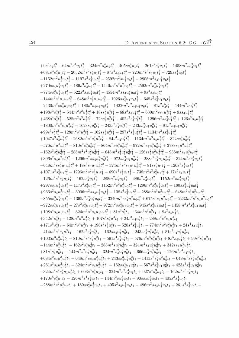
124 D Appendix to Section 6.2: GG→ G t t
+9s5s4t31 − 64m2s4u1t
31 − 324m2s44u1t
31 − 405ss44u1t
31 − 261s2s34u1t
31 − 1458m2ss34u1t
31
+681s3s24u1t31 − 2052m2s2s24u1t
31 + 87s4s4u1t
31 − 720m2s3s4u1t
31 − 729ss44u6t
31
−1152m2u41u6t
31 − 1197s2s34u6t
31 − 2592m2su3
1u6t31 − 2808m2s4u
31u6t
31
+270ss4u31u6t
31 − 189s3s24u6t
31 − 1440m2s2u2
1u6t31 − 2592m2s24u
21u6t
31
−774ss24u21u6t
31 + 522s2s4u
21u6t
31 − 4554m2ss4u
21u6t
31 + 9s4s4u6t
31
−144m2s3u1u6t31 − 648m2s34u1u6t
31 − 1926ss34u1u6t
31 − 648s2s24u1u6t
31
−2430m2ss24u1u6t31 + 180s3s4u1u6t
31 − 1422m2s2s4u1u6t
31 − 81s2s54t
21 − 144m2su5
1t21
+198s3s44t21 − 544m2s2u4
1t21 + 18ss24u
41t
21 + 68s2s4u
41t
21 − 630m2ss4u
41t
21 + 9ss4u
51t
21
+468s4s34t21 − 528m2s3u3
1t21 − 72ss34u
31t
21 + 402s2s24u
31t
21 − 1296m2ss24u
31t
21 + 126s3s4u
31t
21
−1800m2s2s4u31t
21 − 162ss34u
36t
21 − 243s2s24u
36t
21 − 243ss24u1u
36t
21 − 81s2s4u1u
36t
21
+99s5s24t21 − 128m2s4u2
1t21 − 162ss44u
21t
21 + 297s2s34u
21t
21 − 1134m2ss34u
21t
21
+1047s3s24u21t
21 − 2682m2s2s24u
21t
21 + 84s4s4u
21t
21 − 1134m2s3s4u
21t
21 − 324ss44u
26t
21
−576m2u41u
26t
21 − 810s2s34u
26t
21 − 864m2su3
1u26t
21 − 972m2s4u
31u
26t
21 + 378ss4u
31u
26t
21
−162s3s24u26t
21 − 288m2s2u2
1u26t
21 − 648m2s24u
21u
26t
21 − 126ss24u
21u
26t
21 − 936m2s4u
41u6t
21
+396s2s4u21u
26t
21 − 1296m2ss4u
21u
26t
21 − 972ss34u1u
26t
21 − 288s2s24u1u
26t
21 − 324m2ss44u1t
21
−648m2ss24u1u26t
21 + 18s3s4u1u
26t
21 − 324m2s2s4u1u
26t
21 − 81ss54u1t
21 − 126s2s44u1t
21
+1071s3s34u1t21 − 1296m2s2s34u1t
21 + 690s4s24u1t
21 − 738m2s3s24u1t
21 + 17s5s4u1t
21
−126m2s4s4u1t21 − 162ss54u6t
21 − 288m2u5
1u6t21 − 486s2s44u6t
21 − 1152m2su4
1u6t21
+297ss4u41u6t
21 + 117s3s34u6t
21 − 1152m2s2u3
1u6t21 − 1296m2s24u
31u6t
21 + 180ss24u
31u6t
21
+936s2s4u31u6t
21 − 3006m2ss4u
31u6t
21 + 108s4s24u6t
21 − 288m2s3u2
1u6t21 − 648m2s34u
21u6t
21
−855ss34u21u6t
21 + 1395s2s24u
21u6t
21 − 3240m2ss24u
21u6t
21 + 675s3s4u
21u6t
21 − 2232m2s2s4u
21u6t
21
−972ss44u1u6t21 − 27s2s34u1u6t
21 − 972m2ss34u1u6t
21 + 945s3s24u1u6t
21 − 1458m2s2s24u1u6t
21
+108s4s4u1u6t21 − 324m2s3s4u1u6t
21 + 81s3s54t1 − 64m2s2u5
1t1 + 8s2s4u51t1
+342s4s44t1 − 128m2s3u41t1 + 107s2s24u
41t1 + 24s3s4u
41t1 − 288m2s2s4u
41t1
+171s5s34t1 − 64m2s4u31t1 + 198s2s34u
31t1 + 528s3s24u
31t1 − 774m2s2s24u
31t1 + 24s4s4u
31t1
−414m2s3s4u31t1 − 162s2s34u
36t1 + 162ss4u
31u
36t1 + 243ss24u
21u
36t1 + 81s2s4u
21u
36t1
+1035s3s34u21t1 − 810m2s2s34u
21t1 + 591s4s24u
21t1 − 576m2s3s24u
21t1 + 8s5s4u
21t1 + 99s2s44u
21t1
−144m2u51u
26t1 − 162s2s44u
26t1 − 288m2su4
1u26t1 − 324m2s4u
41u
26t1 + 342ss4u
41u
26t1
+81s3s34u26t1 − 144m2s2u3
1u26t1 − 324m2s24u
31u
26t1 + 666ss24u
31u
26t1 − 126m2s4s4u
21t1
+684s2s4u31u
26t1 − 648m2ss4u
31u
26t1 + 243ss34u
21u
26t1 + 1413s2s24u
21u
26t1 − 648m2ss24u
21u
26t1
+261s3s4u21u
26t1 − 324m2s2s4u
21u
26t1 − 162ss44u1u
26t1 + 567s2s34u1u
26t1 + 423s3s24u1u
26t1
−324m2s2s24u1u26t1 + 603s3s44u1t1 − 324m2s2s44u1t1 + 927s4s34u1t1 − 162m2s3s34u1t1
+170s5s24u1t1 − 126m2s4s24u1t1 − 144m2su51u6t1 + 90ss4u
51u6t1 + 405s3s44u6t1
−288m2s2u41u6t1 + 189ss24u
41u6t1 + 495s2s4u
41u6t1 − 486m2ss4u
41u6t1 + 261s4s34u6t1−

D.3 Squared Amplitudes 125
−144m2s3u31u6t1 + 18ss34u
31u6t1 + 1476s2s24u
31u6t1 − 810m2ss24u
31u6t1 + 576s3s4u
31u6t1
−810m2s2s4u31u6t1 − 243ss44u
21u6t1 + 1638s2s34u
21u6t1 − 324m2ss34u
21u6t1
+1710s3s24u21u6t1 − 1134m2s2s24u
21u6t1 + 171s4s4u
21u6t1
−324m2s3s4u21u6t1 − 162ss54u1u6t1 + 567s2s44u1u6t1 + 1638s3s34u1u6t1
−324m2s2s34u1u6t1 + 423s4s24u1u6t1 − 324m2s3s24u1u6t1 + 81s4s54
+81s5s44 + 72s3s24u41 + 234s3s34u
31 + 144s4s24u
31 + 81ss4u
41u
36 + 243ss24u
31u
36
+81s2s4u31u
36 + 162ss34u
21u
36 + 243s2s24u
21u
36 + 162s2s34u1u
36
+243s3s44u21 + 387s4s34u
21 + 72s5s24u
21 + 81ss4u
51u
26 + 162s3s44u
26
+243ss24u41u
26 + 243s2s4u
41u
26 + 324ss34u
31u
26 + 810s2s24u
31u
26
+162s3s4u31u
26 + 162ss44u
21u
26 + 891s2s34u
21u
26 + 567s3s24u
21u
26
+324s2s44u1u26 + 567s3s34u1u
26 + 81s3s54u1 + 324s4s44u1 + 153s5s34u1
+162s3s54u6 + 72s2s4u51u6 + 162s4s44u6 + 297s2s24u
41u6 + 144s3s4u
41u6
+630s2s34u31u6 + 594s3s24u
31u6 + 72s4s4u
31u6 + 567s2s44u
21u6
+1017s3s34u21u6 + 297s4s24u
21u6 + 162s2s54u1u6 + 729s3s44u1u6 +387s4s34u1u6
)
List of Tables
3.1 Particle Content of the MSSM . . . . . . . . . . . . . . . . . . . . . . . . . . . . 213.2 Degrees of Freedom . . . . . . . . . . . . . . . . . . . . . . . . . . . . . . . . . . . 23
A.1 Feynman Rules for QCD . . . . . . . . . . . . . . . . . . . . . . . . . . . . . . . . 81A.2 Feynman Rules for SUSY QCD . . . . . . . . . . . . . . . . . . . . . . . . . . . . 82A.3 Feynman Rules for Gluons, Quarks, Squarks, Fermions and ε Scalars . . . . . . . 83A.4 Propagators for Scalar, Gluon, ε Scalar and Fermion . . . . . . . . . . . . . . . . 83A.5 BRST Ghost Propagator and Vertex . . . . . . . . . . . . . . . . . . . . . . . . . 84
List of Figures
1.1 Self Energy of Higgs and Fermion . . . . . . . . . . . . . . . . . . . . . . . . . . . 2
2.1 Deep Inelastic Scattering . . . . . . . . . . . . . . . . . . . . . . . . . . . . . . . . 6
2.2 Collinear Gluon Emission . . . . . . . . . . . . . . . . . . . . . . . . . . . . . . . 8
2.3 Illustration of the auxiliary Vector n . . . . . . . . . . . . . . . . . . . . . . . . . 9
2.4 Double Collinear Splitting . . . . . . . . . . . . . . . . . . . . . . . . . . . . . . . 14
2.5 HERA Measurements . . . . . . . . . . . . . . . . . . . . . . . . . . . . . . . . . 15
2.6 SLAC Experiments . . . . . . . . . . . . . . . . . . . . . . . . . . . . . . . . . . . 16
2.7 PDFs for the Up Quark . . . . . . . . . . . . . . . . . . . . . . . . . . . . . . . . 17
2.8 PDFs for Partons . . . . . . . . . . . . . . . . . . . . . . . . . . . . . . . . . . . . 18
4.1 Notation for Momenta, Color indices and Lorentz indices . . . . . . . . . . . . . 30
4.2 Naming Conventions for the Collinear Particles . . . . . . . . . . . . . . . . . . . 34
5.1 Feynman Diagram for qq → t t . . . . . . . . . . . . . . . . . . . . . . . . . . . . 40
5.2 Feynman Diagrams for gg → t t . . . . . . . . . . . . . . . . . . . . . . . . . . . . 43
5.3 Feynman Diagrams for BRST Ghosts ηη → t t and ηη → t t . . . . . . . . . . . . 43
5.4 Feynman Diagrams for φφ→ t t . . . . . . . . . . . . . . . . . . . . . . . . . . . . 44
6.1 Feynman Diagrams for qq → Gt t . . . . . . . . . . . . . . . . . . . . . . . . . . . 48
6.2 Redefinition of Mandelstam Variables . . . . . . . . . . . . . . . . . . . . . . . . 50
6.3 Feynman Diagrams for qq → φ t t . . . . . . . . . . . . . . . . . . . . . . . . . . . 53
6.4 Feynman Diagrams for GG→ G t t . . . . . . . . . . . . . . . . . . . . . . . . . . 54
6.5 Schematic Diagrams for the Ghost Processes Corresponding to GG→ G t t . . . 61
6.6 Schematic Diagrams for gg → gt t . . . . . . . . . . . . . . . . . . . . . . . . . . . 65
6.7 All Schematic NLO Diagrams with their Corresponding LO Processes. . . . . . . 66
7.1 Feynman Diagrams for qq → tt . . . . . . . . . . . . . . . . . . . . . . . . . . . . 73
7.2 Feynman Diagrams for gg → tt . . . . . . . . . . . . . . . . . . . . . . . . . . . . 74
A.1 Definition of Mandelstam Variables for 4 and 5 External Legs . . . . . . . . . . . 78
D.1 Feynman Diagrams Involving BRST Ghosts for GG→ G t t . . . . . . . . . . . . 92
D.2 Feynman Diagrams Involving BRST Ghosts GG→ g t t . . . . . . . . . . . . . . 93
D.3 Feynman Diagrams for GG→ Gtt . . . . . . . . . . . . . . . . . . . . . . . . . . 94

128 List of Figures
D.4 Feynman Diagrams for φ g → φ t t . . . . . . . . . . . . . . . . . . . . . . . . . . . 95
D.5 Feynman Diagrams for g φ→ φ t t . . . . . . . . . . . . . . . . . . . . . . . . . . . 96
D.6 Feynman Diagrams for φφ→ g t t . . . . . . . . . . . . . . . . . . . . . . . . . . . 97D.7 Denotation of the Momenta, Lorentz and Color Indices. . . . . . . . . . . . . . . 98

Bibliography
[1] W. Beenakker, H. Kuijf, W. L. van Neerven, and J. Smith. QCD corrections to heavy quarkproduction in p anti-p collisions. Phys. Rev., D40:54–82, 1989.
[2] Adrian Signer and Dominik Stockinger. Factorization and regularization by dimensionalreduction. Phys. Lett., B626:127–138, 2005.
[3] Stephen P. Martin. A supersymmetry primer. 1997.
[4] W. M. Yao et al. Review of particle physics. J. Phys., G33:1–1232, 2006.
[5] Gerard ’t Hooft and M. J. G. Veltman. Regularization and renormalization of gauge fields.Nucl. Phys., B44:189–213, 1972.
[6] W. Beenakker, R. Hopker, and P. M. Zerwas. Susy-QCD decays of squarks and gluinos.Phys. Lett., B378:159–166, 1996.
[7] W. Hollik, E. Kraus, and D. Stockinger. Renormalization of supersymmetric yang-millstheories with soft supersymmetry breaking. Eur. Phys. J., C23:735–747, 2002.
[8] W. Hollik and D. Stockinger. Regularization and supersymmetry-restoring counterterms insupersymmetric QCD. Eur. Phys. J., C20:105–119, 2001.
[9] I. Fischer, W. Hollik, M. Roth, and D. Stockinger. Restoration of supersymmetric slavnov-taylor and ward identities in presence of soft and spontaneous symmetry breaking. Phys.Rev., D69:015004, 2004.
[10] Warren Siegel. Supersymmetric dimensional regularization via dimensional reduction. Phys.Lett., B84:193, 1979.
[11] D. M. Capper, D. R. T. Jones, and P. van Nieuwenhuizen. Regularization by dimensionalreduction of supersymmetric and nonsupersymmetric gauge theories. Nucl. Phys., B167:479,1980.
[12] Dominik Stockinger. Regularization by dimensional reduction: Consistency, quantum ac-tion principle, and supersymmetry. JHEP, 03:076, 2005.
[13] Robert V. Harlander and Franziska Hofmann. Pseudo-scalar higgs production at next-to-leading order susy-QCD. JHEP, 03:050, 2006.
130 Bibliography
[14] D. J. Gross and Frank Wilczek. Ultraviolet behavior of non-abelian gauge theories. Phys.Rev. Lett., 30:1343–1346, 1973.
[15] H. David Politzer. Reliable perturbative results for strong interactions? Phys. Rev. Lett.,30:1346–1349, 1973.
[16] John C. Collins and Davison E. Soper. The theorems of perturbative QCD. Ann. Rev.Nucl. Part. Sci., 37:383–409, 1987.
[17] R. Keith Ellis, W. James Stirling, and B. R. Webber. QCD and collider physics, volume 8.Camb. Monogr. Part. Phys. Nucl. Phys. Cosmol., 1996.
[18] M. Bohm, Ansgar Denner, and H. Joos. Gauge theories of the strong and electroweakinteraction. Stuttgart, Germany: Teubner (2001) 784 p, 2001.
[19] Stefano Catani, Stefan Dittmaier, and Zoltan Trocsanyi. One-loop singular behaviour ofQCD and susy QCD amplitudes with massive partons. Phys. Lett., B500:149–160, 2001.
[20] The q → q splitting function, http://hepwww.rl.ac.uk/theory/seymour/work/busstepp1.ps z,2007.
[21] S. Chekanov et al. Measurement of the neutral current cross section and f2 structurefunction for deep inelastic e+ p scattering at hera. Eur. Phys. J., C21:443–471, 2001.
[22] Jerome I. Friedman and Henry W. Kendall. Deep inelastic electron scattering. Ann. Rev.Nucl. Part. Sci., 22:203–254, 1972.
[23] Guido Altarelli and G. Parisi. Asymptotic freedom in parton language. Nucl. Phys.,B126:298, 1977.
[24] Yuri L. Dokshitzer. Calculation of the structure functions for deep inelastic scattering ande+ e- annihilation by perturbation theory in quantum chromodynamics. (in russian). Sov.Phys. JETP, 46:641–653, 1977.
[25] V. N. Gribov and L. N. Lipatov. Deep inelastic e p scattering in perturbation theory. Sov.J. Nucl. Phys., 15:438–450, 1972.
[26] Mathematica package for cteq pdfs, http://www.phys.psu.edu/ cteq/, 2007.
[27] J. Wess and B. Zumino. Supergauge transformations in four-dimensions. Nucl. Phys.,B70:39–50, 1974.
[28] Michael E. Peskin and D. V. Schroeder. An Introduction to quantum field theory. Reading,USA: Addison-Wesley (1995) 842 p, 1995.
[29] W. Beenakker, R. Hopker, M. Spira, and P. M. Zerwas. Squark and Gluino Production atHadron Colliders. Nucl. Phys., B492:51–103, 1997.
Bibliography 131
[30] Zoltan Kunszt, Adrian Signer, and Zoltan Trocsanyi. One loop helicity amplitudes for all 2→ 2 processes in QCD and n=1 supersymmetric yang-mills theory. Nucl. Phys., B411:397–442, 1994.
[31] Tilman Plehn. Phd thesis: Production of supersymmetric praticles at high-energy colliders.Master’s thesis, Universitat Hamburg, 1998.
[32] Helmut Eberl. Dissertation: Strahlungskorrekturen im minimalen SupersymmetrischenStandardmodell. Master’s thesis, Technische Universitat Wien, 1998.
[33] FeynArts Manual, http://www.feynarts.de/fa3guide.ps.gz, 2007.
[34] FormCalc Manual, http://www.feynarts.de/formcalc/fc5guide.ps.gz, 2007.
Danksagung
Auf der letzten Seite angelangt, mochte ich mich noch bei allen Menschen bedanken, die michin der Zeit meines Studiums und der Diplomarbeit motiviert und unterstutzt haben.Als Erstes danke ich Alex, dass man mit ihm mal eben am Badspiegel uber Supersymmetrie undschwarze Locher diskutieren kann, dass es ihm nicht auf die Nerven geht, dass ich zwei Burosnebenan sitze, und fur seine unglaubliche Geduld in der letzten Zeit. Außerdem danke ich ihmnaturlich fur das Korrekturlesen der Arbeit.Ich mochte meinem Betreuer Prof. Dr. Werner Porod fur die Aufnahme in seine Arbeitsgruppe,die interessante Problemstellung und die Unterstutzung bei der Anfertigung der Arbeit danken.Er hatte immer eine offene Tur fur mich, um mit mir meine (manchmal zahlreichen) Fragen zudiskutieren.PD Dr. Thorsten Ohl danke ich fur viele hilfreiche Diskussionen und seine Art, mich zu mo-tivieren. Prof. Dr. Reinhold Ruckl danke ich fur den interessanten und beeindruckenden Einstiegin die Quantenfeldtheorie und die Teilchenphysik.Ein besonderer Dank gebuhrt auch Christian Speckner, einmal fur seine Umsorge und Hilfebezuglich aller Computerangelegenheiten und fur sein offenes Ohr bei vielen Fragen. BarbaraDubanek danke ich fur das geduldige Korrekturlesen. Ihnen und Martin Schroter mochte ichauch fur die notige Zerstreuung an schonen, langen Abenden und in (notwendigen) Kaffeepausendanken.Außerdem mochte ich mich bei meinen Eltern bedanken, die mir Ruckhalt und ein offenes Ohrfur die unterschiedlichsten Probleme gegeben haben und es wunderbar verstanden haben, michzu den richtigen Zeiten aufzuheitern und abzulenken. Auch Robert mochte ich dafur danken,dass er mich (vor langer Zeit in Spielbach) mit seiner Begeisterung fur Astronomie und astro-physikalische Vorgange angesteckt hat.
Erklarung
Hiermit erklare ich, dass ich die vorliegende Arbeit selbststandig verfasst und keine anderen alsdie angegebenen Hilfsmittel verwendet habe.
Wurzburg, den 27. September 2007
Lisa Edelhauser


![Space-like (vs. time-like) collinear limits in QCD: is ...tudes. In the case of one-loop QCD amplitudes, collinear factorization was introduced in Refs. [23, 24, 12, 25], by explicitly](https://img.pdfslide.us/doc/110x75/60f3bcdb5de38941ac3d3fe5/space-like-vs-time-like-collinear-limits-in-qcd-is-tudes-in-the-case-of.jpg)


![SUSY+beyond - tfc.tohoku.ac.jp · EWSB by TeV dynamics and elementary Higgs for fermion masses. SUSY protects the Higgs mass. ... between Dirac monopoles. [JLQCD ’08] lattice QCD](https://img.pdfslide.us/doc/110x75/613aa7e10051793c8c012a47/susybeyond-tfc-ewsb-by-tev-dynamics-and-elementary-higgs-for-fermion-masses.jpg)

![spiky BA - Career Account Web Pagesweb.ics.purdue.edu/~markru/talks/spiky_BA.pdf · ( Susy, 10d, Q.G. ) QCD [ SU(3) ] ... Generalization to higher twist operators (MK) O Trn ... Microsoft](https://img.pdfslide.us/doc/110x75/5b3338567f8b9aae458c8c10/spiky-ba-career-account-web-markrutalksspikybapdf-susy-10d-qg-.jpg)