Mass and Heat Transfer During Two-Phase Flow in …cdn.intechweb.org/pdfs/13526.pdfMass and Heat Transfer During Two-Phase Flow in Porous Media - Theory and Modeling 3 (a) Carbon capture

0

Mass and Heat Transfer During Two-Phase Flow inPorous Media - Theory and Modeling

Jennifer Niessner1 and S. Majid Hassanizadeh2

1Institute of Hydraulic Engineering, University of Stuttgart, Stuttgart2Department of Earth Sciences, Faculty of Geosciences, Utrecht University, Utrecht

1Germany2The Netherlands

1. Introduction

1.1 Motivation

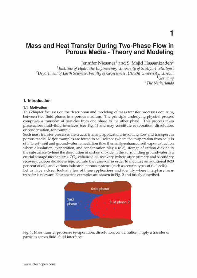
This chapter focusses on the description and modeling of mass transfer processes occurringbetween two fluid phases in a porous medium. The principle underlying physical processcomprises a transport of particles from one phase to the other phase. This process takesplace across fluid–fluid interfaces (see Fig. 1) and may constitute evaporation, dissolution,or condensation, for example.Such mass transfer processes are crucial in many applications involving flow and transport inporous media. Major examples are found in soil science (where the evaporation from soils isof interest), soil and groundwater remediation (like thermally-enhanced soil vapor extractionwhere dissolution, evaporation, and condensation play a role), storage of carbon dioxide inthe subsurface (where the dissolution of carbon dioxide in the surrounding groundwater is acrucial storage mechanism), CO2-enhanced oil recovery (where after primary and secondaryrecovery, carbon dioxide is injected into the reservoir in order to mobilize an additional 8-20per cent of oil), and various industrial porous systems (such as certain types of fuel cells).Let us have a closer look at a few of these applications and identify where interphase masstransfer is relevant. Four specific examples are shown in Fig. 2 and briefly described.

solid phase

fluid

phase 1fluid phase 2

Fig. 1. Mass transfer processes (evaporation, dissolution, condensation) imply a transfer ofparticles across fluid–fluid interfaces.

1

www.intechopen.com

2 Mass Transfer

(a) Carbon dioxide storage in the subsurface(figure from IPCC (2005))

(b) Soil contamination and remediation

(c) Enhanced oil recovery (figure fromwww.oxy.com)

groundwater

precipitationradiation

evaporation

infiltration

(d) Evaporation from soil

Fig. 2. Four applications of flow and transport in porous media where interphase masstransfer is important

2 Mass Transfer in Multiphase Systems and its Applications

www.intechopen.com

Mass and Heat Transfer During Two-Phase Flow in Porous Media - Theory and Modeling 3

(a) Carbon capture and storage (Fig. 2 (a)) is a recent strategy to mitigate the greenhouseeffect by capturing the greenhouse gas carbon dioxide that is emitted e.g. by coal powerplants and inject it directly into the subsurface below an impermeable caprock. Here, threedifferent storage mechanisms are relevant on different time scales: 1) The capillary barriermechanism of the caprock. This geologic layer is meant to keep the carbon dioxide in thestorage reservoir as a separate phase. 2) Dissolution of the carbon dioxide in the surroundingbrine (salty groundwater). This is a longterm storage mechanism and involves a masstransfer process as carbon dioxide molecules are “transferred” from the gaseous phase tothe brine phase. 3) Geochemical reactions which immobilize the carbon dioxide throughincorporation into the rock matrix.

(b) Shown in Fig. 2 (b) is a cartoon of a light non-aqueous phase liquid (LNAPL)soil contamination and its clean up by injection of steam at wells located around thecontaminated soil. The idea behind this strategy is to mobilize the initially immobile(residual) LNAPL by evaporation of LNAPL component at large rates into the gaseousphase. The soil gas is then extracted by a centrally located extraction well. It means that theremediation mechanism relies on the evaporation of LNAPL component which represents amass transfer from the liquid LNAPL phase into the gaseous phase.

(c) In order to produce an additional 8-20% of oil after primary and secondary recovery,carbon dioxide may be injected into an oil reservoir, e.g. alternatingly with water, seeFig. 2 (c). This is called enhanced oil recovery. The advantage of injecting carbon dioxide liesin the fact that it dissolves in the oil which in turn reduces the oil viscosity, and thus, increasesits mobility. The improved mobility of the oil allows for an extraction of the otherwisetrapped oil. Here, an interphase mass transfer process (dissolution) is responsible for animproved recovery.

(d) The last example (Fig. 2 (d)) shows the upper part of the soil. The water balance of this partof the subsurface is extremely important for agriculture or plant growth in general. Plantsdo not grow well under too wet or too dry conditions. One of the very important factorsinfluencing this water balance (besides surface runoff and infiltration) is the evaporation ofwater from the soil, which is again an interphase mass transfer process.

1.2 Purpose of this work

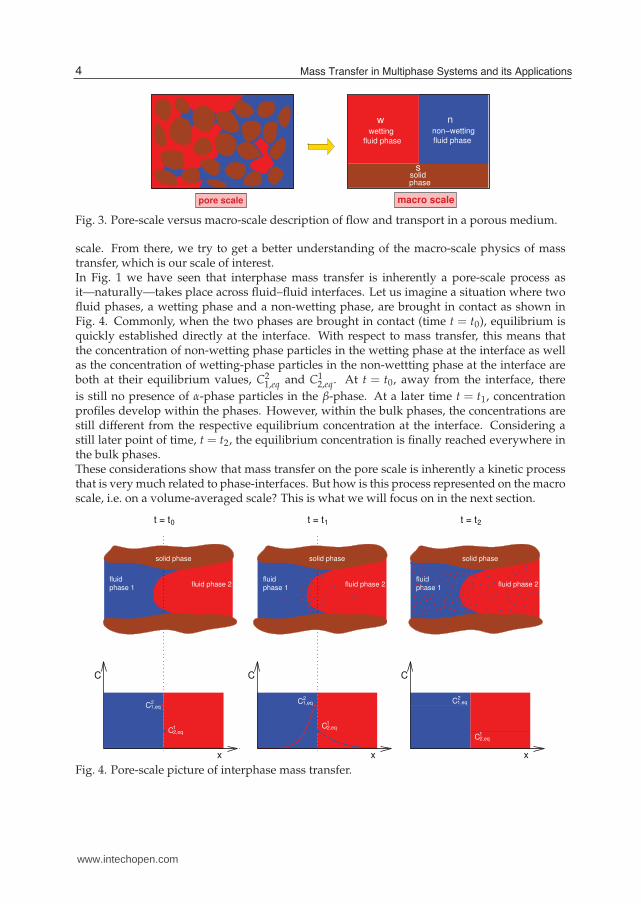
Mass transfer processes are essential in a large variety of applications—the presentedexamples only show a small selection of systems. A common feature of all these applications isthe fact that the relevant processes occur in relatively large domains such that it is not possibleto resolve the pore structure and the fluid distribution in detail (left hand side of Fig. 3).Instead, a macro-scale approach is needed where properties and processes are averaged overa so-called representative elementary volume (right hand side of Fig. 3). This means that thecommon challenge in all of the above-mentioned applications is how to describe mass transferprocesses on a macro scale. This transition from the pore scale to the macro scale is illustratedin Fig. 3 where on the left side, the pore-scale situation is shown (which is impossible to beresolved in detail) while on the right hand side, the macro-scale situation is shown.

2. Overview of classical mass transfer descriptions

2.1 Pore-scale considerations

In order to better understand the physics of interphase mass transfer, which is essential toprovide a physically-based description of this process, we start our considerations on the pore

3Mass and Heat Transfer During Two-Phase Flow in Porous Media - Theory and Modeling

www.intechopen.com

4 Mass Transfer

ssolidphase

wwetting

fluid phase

nnon−wetting

fluid phase

pore scale macro scale

Fig. 3. Pore-scale versus macro-scale description of flow and transport in a porous medium.

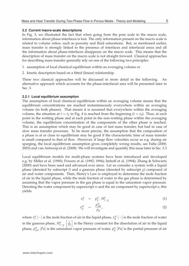
scale. From there, we try to get a better understanding of the macro-scale physics of masstransfer, which is our scale of interest.In Fig. 1 we have seen that interphase mass transfer is inherently a pore-scale process asit—naturally—takes place across fluid–fluid interfaces. Let us imagine a situation where twofluid phases, a wetting phase and a non-wetting phase, are brought in contact as shown inFig. 4. Commonly, when the two phases are brought in contact (time t = t0), equilibrium isquickly established directly at the interface. With respect to mass transfer, this means thatthe concentration of non-wetting phase particles in the wetting phase at the interface as wellas the concentration of wetting-phase particles in the non-wettting phase at the interface areboth at their equilibrium values, C2

1,eq and C12,eq. At t = t0, away from the interface, there

is still no presence of α-phase particles in the β-phase. At a later time t = t1, concentrationprofiles develop within the phases. However, within the bulk phases, the concentrations arestill different from the respective equilibrium concentration at the interface. Considering astill later point of time, t = t2, the equilibrium concentration is finally reached everywhere inthe bulk phases.These considerations show that mass transfer on the pore scale is inherently a kinetic processthat is very much related to phase-interfaces. But how is this process represented on the macroscale, i.e. on a volume-averaged scale? This is what we will focus on in the next section.

C12,eq

C21,eq

C12,eq

solid phase

fluid


C

C21,eq

12,eq

C

x

t = t0

solid phase

fluid


C

x

t = t1

solid phase

fluid


C

x

t = t2

C21,eq

Fig. 4. Pore-scale picture of interphase mass transfer.


www.intechopen.com


2.2 Current macro-scale descriptions

In Fig. 3, we illustrated the fact that when going from the pore scale to the macro scale,information about phase-interfaces is lost. The only information present on the macro scale isrelated to volume ratios, such as porosity and fluid saturations. But, as mentioned earlier,mass transfer is strongly linked to the presence of interfaces and interfacial areas and allthe information about phase-interfaces disappears on the macro scale. This means that thedescription of mass transfer on the macro scale is not straight forward. Classical approachesfor describing mass transfer generally rely on one of the following two principles:

1. assumption of local chemical equilibrium within an averaging volume or

2. kinetic description based on a fitted (linear) relationship.

These two classical approaches will be discussed in more detail in the following. Analternative approach which accounts for the phase-interfacial area will be presented later inSec. 3.

2.2.1 Local equilibrium assumption

The assumption of local chemical equilibrium within an averaging volume means that theequilibrium concentrations are reached instantaneously everywhere within an averagingvolume (in both phases). That means it is assumed that everywhere within the averagingvolume, the situation at t = t2 in Fig. 4 is reached from the beginning (t = t0). Thus, at eachpoint in the wetting phase and at each point in the non-wetting phase within the averagingvolume, the equilibrium concentration of the components of the other phase is reached.This is an assumption which may be good in case of fast mass transfer, but bad in case ofslow mass transfer processes. To be more precise, the assumption that the composition ofa phase is at or close to equilibrium may be good if the characteristic time of mass transferis small compared to that of flow. However, if large flow velocities occur as e.g. during airsparging, the local equilibrium assumption gives completely wrong results, see Falta (2000;2003) and van Antwerp et al. (2008). We will investigate and quantify this issue later in Sec. 3.3.Local equilibrium models for multi-phase systems have been introduced and developede.g. by Miller et al. (1990); Powers et al. (1992; 1994); Imhoff et al. (1994); Zhang & Schwartz(2000) and have been used and advanced ever since. Let us consider a system with a liquidphase (denoted by subscript l) and a gaseous phase (denoted by subscript g) composed ofair and water components. Then, Henry’s Law is employed to determine the mole fractionof air in the liquid phase, while the mole fraction of water in the gas phase is determined byassuming that the vapor pressure in the gas phase is equal to the saturation vapor pressure.Denoting the water component by superscript w and the air component by superscript a, thisyields

xal = pa

g · Hal−g (1)

xwg =

pwsat

pg, (2)

where xal [−] is the mole fraction of air in the liquid phase, xw

g [−] is the mole fraction of water

in the gaseous phase, Hal−g

[

1Pa

]

is the Henry constant for the dissolution of air in the liquid

phase, pwsat [Pa] is the saturation vapor pressure of water, pa

g [Pa] is the partial pressure of air


www.intechopen.com

6 Mass Transfer

in the gas phase while pg [Pa] is the gas pressure. The remaining mole fractions result simplyfrom the condition that mole fractions in each phase have to sum up to one,

xwl = 1 − xa

l (3)

xag = 1 − xw

g . (4)

Note that while for a number of applications the equilibrium mole fractions are constants ormerely a function of temperature, in our case, they will be functions of space and time aspressure and the composition of the phases changes.

2.2.2 Classical kinetic approach

Kinetic mass transfer approaches are traditionally applied to the dissolution of contaminantsin the subsurface which form a separate phase from water, the so-called non-aqueous phaseliquids (NAPLs). If such a non-aqueous phase liquid is heavier than water, it is called“dense non-aqueous phase liquid” or DNAPL. When an immobile lense of DNAPL is presentat residual saturation (i.e. at a saturation which is so low that the phase is immobile) anddissolves into the surrounding groundwater, the kinetics of this mass transfer process usuallyplays an important role: the dissolution of DNAPL is a rate-limited process. This is alsothe case when a pool of DNAPL is formed on an impermeable layer. In these relativelysimple cases, only the mass transfer of a DNAPL component from the DNAPL phase intothe water phase has to be considered. For these cases, classical models acknowledge thefact that the rate of mass transfer is highly dependent (proportional to) interfacial area andassume a first-order rate of kinetic mass transfer between fluid phases in a porous mediumon a macroscopic (i.e. volume-averaged) scale which can be expressed as (see e.g. Mayer &Hassanizadeh (2005)):

Qκα→β = kκ

α→βaαβ(Cκβ,s − Cκ

β), (5)

where Qκα→β

[

kgm3s

]

is the interphase mass transfer rate of component κ from phase α to

phase β, kκα→β

[

ms

]

is the mass transfer rate coefficient, aαβ

[

1m

]

is the specific interfacial

area separating phases α and β, Cκβ,s

[

kgm3

]

is the solubility limit of component κ in phase

β, and finally, Cκβ

[

kgm3

]

is the actual concentration of component κ in phase β. The actual

concentration is not larger than the solubility limit, Cκβ ≤ Cκ

β,s. The case Cκβ = Cκ

β,s corresponds

to the local equilibrium case.In the absence of a physically-based estimate of interfacial area in classical kinetic models, themass transfer coefficient kκ

α→β and the specific interfacial area aαβ are often lumped into one

single parameter (Miller et al. (1990); Powers et al. (1992; 1994); Imhoff et al. (1994); Zhang &Schwartz (2000)). This yields, in a simplified notation,

Q = k(Cs − C). (6)

Here, Cs is the solubility limit of the DNAPL component in water and C is its actual

concentration. The lumped mass transfer coefficient k[

1s

]

is commonly related to a modified

Sherwood number Sh by

k = ShDm

d250

, (7)


www.intechopen.com


where Dm

[

m2

s

]

is the aqueous phase molecular diffusion coefficient, and d50 [m] is the mean

size of the grains. The Sherwood number is then related to Reynold’s number Re and DNAPLsaturation Sn [−] by

Sh = pReqSrn, (8)

where p, q, and r are dimensionless fitting parameters. This is a purely empirical relationship.Although interphase mass transfer is proportional to specific interfacial area in the originalEq. (5), this dependence cannot explicitly be accounted for as the magnitude of specificinterfacial area is not known.An alternative classical approach for DNAPL pool dissolution has been proposed by Falta(2003) who modeled the dissolution of DNAPL component by a dual domain approachfor a case with simple geometry. For this purpose, they divided the contaminated porousmedium into two parts: one that contains DNAPL pools and one without DNAPL. Fortheir simple case, the dual domain approach combined with an analytical solution forsteady-state advection and dispersion provided a means for modeling rate-limited interphasemass transfer. While this approach provided good results for the case of simplified geometry,it might be oversimplified for the modeling of realistic situations.

3. Interfacial-area-based approach for mass transfer description

3.1 Theoretical background

Due to a number of deficiencies of the classical model for two-phase flow in porous media(one of which is the problem in describing kinetic interphase mass transfer on the macroscale), several approaches have been developed to describe two-phase flow in an alternativeand thermodynamically-based way. Among these are a rational thermodynamics approachby Hassanizadeh & Gray (1980; 1990; 1993b;a), a thermodynamically constrained averagingtheory approach by Gray and Miller (e.g. Gray & Miller (2005); Jackson et al. (2009)),mixture theory (Bowen (1982)) and an approach based on averaging and non-equilibriumthermodynamics by Marle (1981) and Kalaydjian (1987). While Marle (1981) and Kalaydjian(1987) developed their set of constitutive relationships phenomenologically, Hassanizadeh &Gray (1990; 1993b); Jackson et al. (2009), and Bowen (1982) exploited the entropy inequalityto obtain constitutive relationships. To the best of our knowledge, the two-phase flow modelsof Marle (1981); Kalaydjian (1987); Hassanizadeh & Gray (1990; 1993b); Jackson et al. (2009)are the only ones to include interfaces explicitly in their formulation allowing to describehysteresis as well as kinetic interphase mass and energy transfer in a physically-based way. Inthe following, we follow the approach of Hassanizadeh & Gray (1990; 1993b) as it includesthe spatial and temporal evolution of phase-interfacial areas as parameters which allowsus to model kinetic interphase mass transfer in a much more physically-based way than isclassically done.It has been conjectured by Hassanizadeh & Gray (1990; 1993b) that problems of the classicaltwo-phase flow model, like the hysteretic behavior of the constitutive relationship betweencapillary pressure and saturation, are due to the absence of interfacial areas in the theory.Hassanizadeh and Gray showed (Hassanizadeh & Gray (1990; 1993b)) that by formulatingthe conservation equations not only for the bulk phases, but additionally for interfaces,and by exploiting the residual entropy inequality, a relationship between capillary pressure,saturation, and specific interfacial areas (interfacial area per volume of REV) can be derived.This relationship has been determined in various experimental works (Brusseau et al. (1997);Chen & Kibbey (2006); Culligan et al. (2004); Schaefer et al. (2000); Wildenschild et al. (2002);


www.intechopen.com

8 Mass Transfer

Chen et al. (2007)) and computational studies (pore-network models and CFD simulationson the pore scale, see Reeves & Celia (1996); Held & Celia (2001); Joekar-Niasar et al. (2008;2009); Porter et al. (2009)). The numerical work of Porter et al. (2009) using Lattice Boltzmansimulations in a glass bead porous medium and experiments of Chen et al. (2007) showthat the relationship between capillary pressure, the specific fluid-fluid interfacial area, andsaturation is the same for drainage and imbibition to within the measurement error. Thisallows for the conclusion that the inclusion of fluid–fluid interfacial area into the capillarypressure–saturation relationship makes hysteresis disappear or, at least, reduces it downto a very small value. Niessner & Hassanizadeh (2008; 2009a;b) have modeled two-phaseflow—using the thermodynamically-based set of equations developed by Hassanizadeh &Gray (1990)—and showed that this interfacial-area-based model is indeed able to modelhysteresis as well as kinetic interphase mass and also energy transfer in a physically-basedway.

3.2 Simplified model

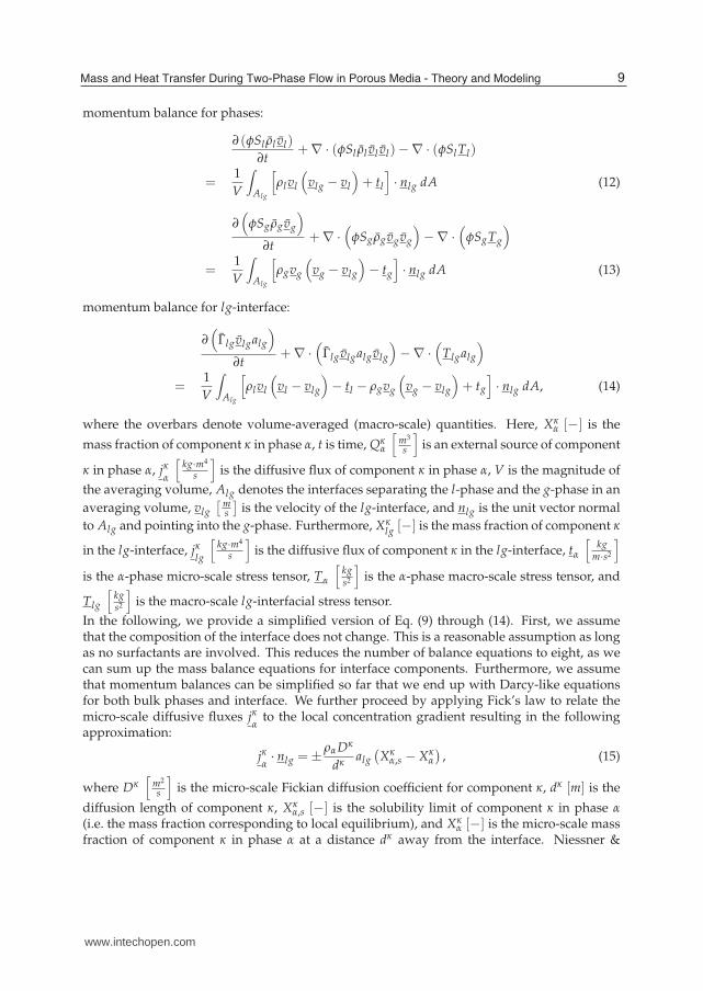
After having presented the general background of our interfacial-area-based model, we willnow proceed by discussing the mathematical model. The complete set of balance equationsbased on the approach of Hassanizadeh & Gray (1990) is too large to be handled numerically.In order to do numerical modeling, simplifying assumptions need to be made. In thefollowing, we present such a simplified equation system as was derived in Niessner &Hassanizadeh (2009a).This set of balance equations can be described by six mass and three momentum balanceequations. These numbers result from the fact that mass balances for each component of eachphase and the fluid–fluid interface (that is 2 × 3) while momentum balances are given for thebulk phases and the interface. Governing equations were derived by Hassanizadeh & Gray(1979) and Gray & Hassanizadeh (1989; 1998) for the case of flow of two pure fluid phaseswith no mass transfer. Extending these equations to the case of two fluid phases, each madeof two components, we obtain the following equations.mass balance for phase components (κ = w, a):

∂(

φSl ρl Xκl

)

∂t+∇ · (φSl ρl X

κl vl)−∇ ·

(

φSl jκ

l

)

= ρl Qκl +

1

V

∫

Alg

[

ρl Xκl

(

vlg − vl

)

+ jκl

]

· nlg dA (9)

∂(

φSg ρgXκg

)

∂t+∇ ·

(

φSg ρgXκg vg

)

−∇ ·

(

φSg jκ

g

)

= ρgQκg +

1

V

∫

Alg

[

ρgXκg

(

vg − vlg

)

− jκg

]

· nlg dA (10)

mass balance for lg-interface components (κ = w, a):

∂(

ΓlgXκlgalg

)

∂t+∇ ·

(

ΓlgXκlgalg vlg

)

−∇ ·

(

jκ

lgalg

)

−

=1

V

∫

Alg

[

ρl Xκl

(

vl − vlg

)

− jκl− ρgXκ

g

(

vg − vlg

)

+ jκg

]

· nlg dA (11)


www.intechopen.com


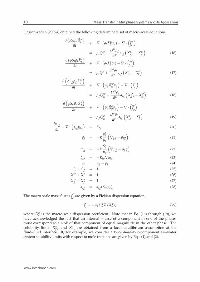
momentum balance for phases:

∂ (φSl ρl vl)

∂t+∇ · (φSl ρl vl vl)−∇ · (φSl Tl)

=1

V

∫

Alg

[

ρlvl

(

vlg − vl

)

+ tl

]

· nlg dA (12)

∂(

φSg ρg vg

)

∂t+∇ ·

(

φSg ρg vg vg

)

−∇ ·

(

φSgTg

)

=1

V

∫

Alg

[

ρgvg

(

vg − vlg

)

− tg

]

· nlg dA (13)

momentum balance for lg-interface:

∂(

Γlg vlgalg

)

∂t+∇ ·

(

Γlg vlgalg vlg

)

−∇ ·

(

Tlgalg

)

=1

V

∫

Alg

[

ρlvl

(

vl − vlg

)

− tl − ρgvg

(

vg − vlg

)

+ tg

]

· nlg dA, (14)

where the overbars denote volume-averaged (macro-scale) quantities. Here, Xκα [−] is the

mass fraction of component κ in phase α, t is time, Qκα

[

m3

s

]

is an external source of component

κ in phase α, jκα

[

kg·m4

s

]

is the diffusive flux of component κ in phase α, V is the magnitude of

the averaging volume, Alg denotes the interfaces separating the l-phase and the g-phase in an

averaging volume, vlg

[

ms

]

is the velocity of the lg-interface, and nlg is the unit vector normal

to Alg and pointing into the g-phase. Furthermore, Xκlg [−] is the mass fraction of component κ

in the lg-interface, jκlg

[

kg·m4

s

]

is the diffusive flux of component κ in the lg-interface, tα

[

kgm·s2

]

is the α-phase micro-scale stress tensor, Tα

[

kgs2

]

is the α-phase macro-scale stress tensor, and

Tlg

[

kgs2

]

is the macro-scale lg-interfacial stress tensor.

In the following, we provide a simplified version of Eq. (9) through (14). First, we assumethat the composition of the interface does not change. This is a reasonable assumption as longas no surfactants are involved. This reduces the number of balance equations to eight, as wecan sum up the mass balance equations for interface components. Furthermore, we assumethat momentum balances can be simplified so far that we end up with Darcy-like equationsfor both bulk phases and interface. We further proceed by applying Fick’s law to relate themicro-scale diffusive fluxes jκ

αto the local concentration gradient resulting in the following

approximation:

jκα· nlg = ±

ραDκ

dκalg

(

Xκα,s − Xκ

α

)

, (15)

where Dκ[

m2

s

]

is the micro-scale Fickian diffusion coefficient for component κ, dκ [m] is the

diffusion length of component κ, Xκα,s [−] is the solubility limit of component κ in phase α

(i.e. the mass fraction corresponding to local equilibrium), and Xκα [−] is the micro-scale mass

fraction of component κ in phase α at a distance dκ away from the interface. Niessner &


www.intechopen.com

10 Mass Transfer

Hassanizadeh (2009a) obtained the following determinate set of macro-scale equations:

∂(

φSl ρl Xwl

)

∂t+ ∇ · (ρl X

wl vl)−∇ ·

(

jw

l

)

= ρl Qwl −

Dw ρg

dwalg

(

Xwg,s − Xw

g

)

(16)

∂(

φSl ρl Xal

)

∂t+ ∇ · (ρl X

al vl)−∇ ·

(

ja

l

)

= ρl Qal +

Da ρl

daalg

(

Xal,s − Xa

l

)

(17)

∂(

φSg ρgXwg

)

∂t+ ∇ ·

(

ρgXwg vg

)

−∇ ·

(

jw

g

)

= ρgQwg +

Dw ρg

dwalg

(

Xwg,s − Xw

g

)

(18)

∂(

φSg ρgXag

)

∂t+ ∇ ·

(

ρgXag vg

)

−∇ ·

(

ja

g

)

= ρgQag −

Da ρl

daalg

(

Xal,s − Xa

l

)

(19)

∂alg

∂t+∇ ·

(

algvlg

)

= Elg (20)

vl = −KS2

l

μl

(

∇pl − ρl g)

(21)

vg = −KS2

g

μg

(

∇pg − ρgg)

(22)

vlg = −Klg∇alg (23)

pc = pg − pl (24)

Sl + Sg = 1 (25)

Xwl + Xa

l = 1 (26)

Xwg + Xa

g = 1 (27)

alg = alg(Sl , pc), (28)

The macro-scale mass fluxes jκ

αare given by a Fickian dispersion equation,

jκ

α= −ραDκ

α∇ (Xκα) , (29)

where Dκα is the macro-scale dispersion coefficient. Note that in Eq. (16) through (19), we

have acknowledged the fact that an internal source of a component in one of the phasesmust correspond to a sink of that component of equal magnitude in the other phase. Thesolubility limits Xw

g,s and Xal,s are obtained from a local equilibrium assumption at the

fluid–fluid interface. If, for example, we consider a two-phase–two-component air–watersystem solubility limits with respect to mole fractions are given by Eqs. (1) and (2).


www.intechopen.com


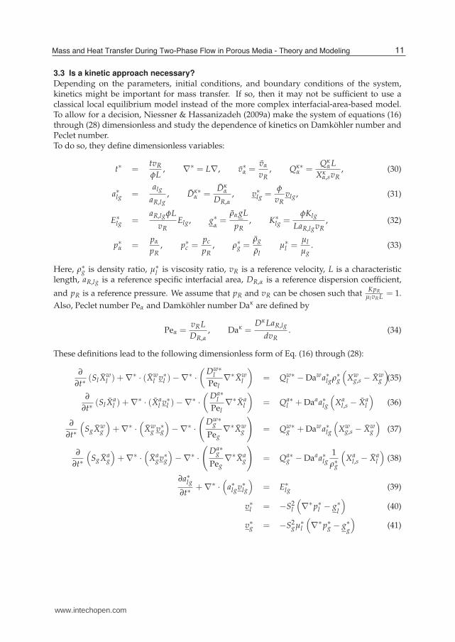
3.3 Is a kinetic approach necessary?

Depending on the parameters, initial conditions, and boundary conditions of the system,kinetics might be important for mass transfer. If so, then it may not be sufficient to use aclassical local equilibrium model instead of the more complex interfacial-area-based model.To allow for a decision, Niessner & Hassanizadeh (2009a) make the system of equations (16)through (28) dimensionless and study the dependence of kinetics on Damkohler number andPeclet number.To do so, they define dimensionless variables:

t∗ =tvR

φL, ∇∗ = L∇, v∗α =

vα

vR, Qκ∗

α =Qκ

αL

Xκα,svR

, (30)

a∗lg =alg

aR,lg, Dκ∗

α =Dκ

α

DR,α, v∗lg =

φ

vRvlg, (31)

E∗lg =

aR,lgφL

vRElg, g∗

α=

ραgL

pR, K∗

lg =φKlg

LaR,lgvR, (32)

p∗α =pα

pR, p∗c =

pc

pR, ρ∗g =

ρg

ρlμ∗

l =μl

μg. (33)

Here, ρ∗g is density ratio, μ∗l is viscosity ratio, vR is a reference velocity, L is a characteristic

length, aR,lg is a reference specific interfacial area, DR,α is a reference dispersion coefficient,

and pR is a reference pressure. We assume that pR and vR can be chosen such thatKpR

μl vR L = 1.

Also, Peclet number Peα and Damkohler number Daκ are defined by

Peα =vRL

DR,α, Daκ =

Dκ LaR,lg

dvR. (34)

These definitions lead to the following dimensionless form of Eq. (16) through (28):

∂

∂t∗(Sl X

wl ) +∇∗ · (Xw

l v∗l )−∇∗ ·

(

Dw∗l

Pel∇∗Xw

l

)

= Qw∗l − Dawa∗lgρ∗g

(

Xwg,s − Xw

g

)

(35)

∂

∂t∗(Sl X

al ) +∇∗ · (Xa

l v∗l )−∇∗ ·

(

Da∗l

Pel∇∗Xa

l

)

= Qa∗l + Daaa∗lg

(

Xal,s − Xa

l

)

(36)

∂

∂t∗

(

SgXwg

)

+∇∗ ·

(

Xwg v∗g

)

−∇∗ ·

(

Dw∗g

Peg∇∗Xw

g

)

= Qw∗g + Dawa∗lg

(

Xwg,s − Xw

g

)

(37)

∂

∂t∗

(

SgXag

)

+∇∗ ·

(

Xagv∗g

)

−∇∗ ·

(

Da∗g

Peg∇∗Xa

g

)

= Qa∗g − Daaa∗lg

1

ρ∗g

(

Xal,s − Xa

l

)

(38)

∂a∗lg

∂t∗+∇∗ ·

(

a∗lgv∗lg

)

= E∗lg (39)

v∗l = −S2l

(

∇∗p∗l − g∗l

)

(40)

v∗g = −S2gμ∗

l

(

∇∗p∗g − g∗g

)

(41)


www.intechopen.com

12 Mass Transfer

v∗lg = −K∗lg∇

∗a∗lg (42)

p∗c = p∗g − p∗l (43)

Sl + Sg = 1 (44)

Xwl + Xa

l = 1 (45)

Xwg + Xa

g = 1 (46)

a∗lg = a∗lg (Sl , p∗c ) . (47)

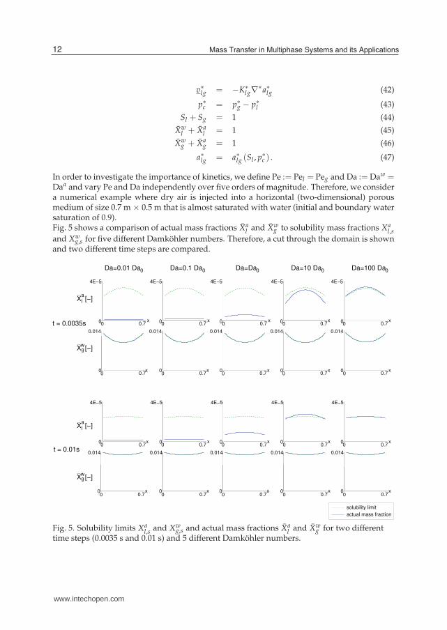
In order to investigate the importance of kinetics, we define Pe := Pel = Peg and Da := Daw =Daa and vary Pe and Da independently over five orders of magnitude. Therefore, we considera numerical example where dry air is injected into a horizontal (two-dimensional) porousmedium of size 0.7 m × 0.5 m that is almost saturated with water (initial and boundary watersaturation of 0.9).Fig. 5 shows a comparison of actual mass fractions Xa

l and Xwg to solubility mass fractions Xa

l,sand Xw

g,s for five different Damkohler numbers. Therefore, a cut through the domain is shownand two different time steps are compared.

0.014

0m 0.7m

t = 0.01s

t = 0.0035s

4.0E-5

0m 0.7m

4.0E-5

0m 0.7m

0.014

0m 0.7m

4.0E-5

0m 0.7m

0.014

0m 0.7m

4.0E-5

0m 0.7m

4.0E-5

0m 0.7m

4.0E-5

0m 0.7m

4.0E-5

0m 0.7m

0.014

0m 0.7m

4.0E-5

0m 0.7m

0.014

0m 0.7m

0.014

0m 0.7m

0.014

0m 0.7m

0.014

0m 0.7m

4.0E-5

0m 0.7m

0.014

0m 0.7m

0.014

0m 0.7m

4.0E-5

0m 0.7m

Da=0.1 Da Da=Da Da=10 Da Da=100 Da

solubility limit

actual mass fraction

l

a

0 0 0 0 0Da=0.01 Da

l

a

wg

wg

X [−]

x x x x x

x

x

x

xxxx

xxxx

xxxx00.70

00 0.7

00 0.7

00 0.7

0.700

0.0140.0140.014 0.014 0.014

00 0.7

0.7000

0 0.700 0.7

00 0.7

00 0.7

0.014 0.014

00 0.7

0.014

00 0.7

0.014

00 0.7

0.014

00 0.7

0 0.70 00 0.7 00 0.7 00 0.7 00 0.7

4E−5 4E−5 4E−5 4E−5 4E−5

X [−]

4E−5 4E−5 4E−5 4E−5 4E−5

X [−]

X [−]

Fig. 5. Solubility limits Xal,s and Xw

g,s and actual mass fractions Xal and Xw

g for two differenttime steps (0.0035 s and 0.01 s) and 5 different Damkohler numbers.


www.intechopen.com


It can be seen that the system is practically instantaneously in equilibrium with respect to themass fraction Xw

g (water mass fraction in the gas phase) for the whole range of consideredDamkohler numbers (see the second and forth row of graphs). With respect to the massfraction Xa

l (air mass fraction in the water phase), for low Damkohler numbers and early times,the system is far from equilibrium (see the first and third row of graphs). With increasingtime and with increasing Damkohler number, the system approaches equilibrium. As forhigh Damkohler numbers mass transfer is very fast, an ”overshoot“ occurs and the systembecomes oversaturated before it reaches equilibrium.One might argue that the considered time steps are extremely small and not relevant for thetime scale relevant for the whole domain. However, what happens at this very early time hasa large influence on the state of the system at all subsequent times.It turned out that for different Peclet numbers, there is no difference in results. That meansthat kinetic interphase mass transfer is independent of Peclet number, at least within the fourorders of magnitude considered here.

4. Extension to heat transfer

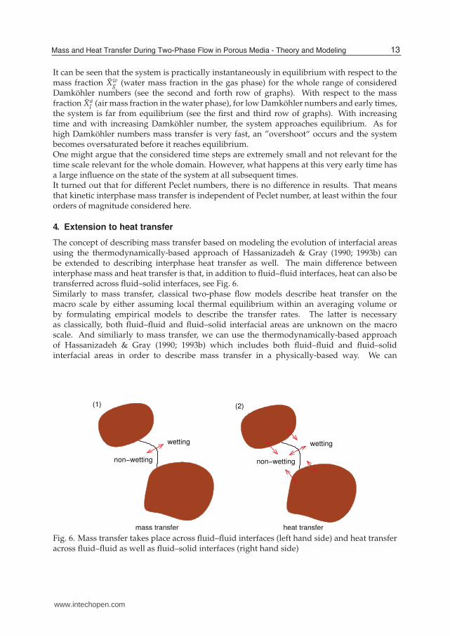
The concept of describing mass transfer based on modeling the evolution of interfacial areasusing the thermodynamically-based approach of Hassanizadeh & Gray (1990; 1993b) canbe extended to describing interphase heat transfer as well. The main difference betweeninterphase mass and heat transfer is that, in addition to fluid–fluid interfaces, heat can also betransferred across fluid–solid interfaces, see Fig. 6.Similarly to mass transfer, classical two-phase flow models describe heat transfer on themacro scale by either assuming local thermal equilibrium within an averaging volume orby formulating empirical models to describe the transfer rates. The latter is necessaryas classically, both fluid–fluid and fluid–solid interfacial areas are unknown on the macroscale. And similiarly to mass transfer, we can use the thermodynamically-based approachof Hassanizadeh & Gray (1990; 1993b) which includes both fluid–fluid and fluid–solidinterfacial areas in order to describe mass transfer in a physically-based way. We can

non−wetting

wetting

(1)

mass transfer

non−wetting

wetting

(2)

heat transfer

Fig. 6. Mass transfer takes place across fluid–fluid interfaces (left hand side) and heat transferacross fluid–fluid as well as fluid–solid interfaces (right hand side)


www.intechopen.com

14 Mass Transfer

also perform a dimensional analysis and derive dimensionless numbers that help to decidewhether kinetics of heat transfer needs to be accounted for or whether a local equilibriummodel is sufficiently accurate on the macro scale. For more details on these issues, we referto Niessner & Hassanizadeh (2009b).

5. Macro-scale example simulations

For the numerical solution of the system of Eq.s (16) through (28), we use a fully-coupledvertex-centered finite element method (an in-house code) which not only conserves masslocally, but is also applicable to unstructured grids. For time discretization, a fully implicitEulerian approach is used, see e.g. Bastian et al. (1997); Bastian & Helmig (1999). The nonlinearsystem is linearized using a damped inexact Newton-Raphson solver, and the linear systemis subsequently solved using a Bi-Conjugate Gradient Stabilized method (known as BiCGStabmethod). Full upwinding is applied to the flux terms of the bulk phase equations, but in theinterfacial area flux term, central weighting is used.

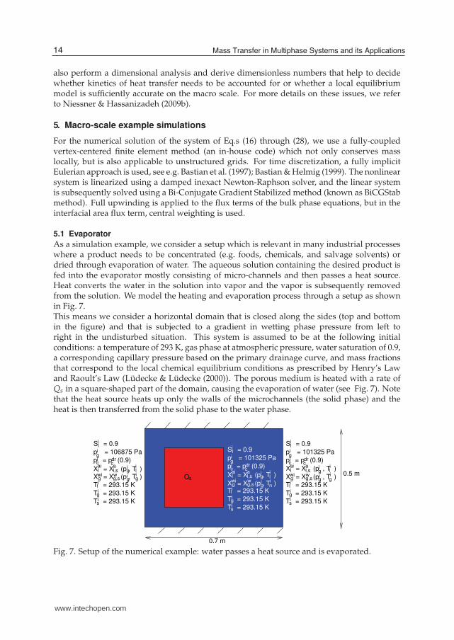
5.1 Evaporator

As a simulation example, we consider a setup which is relevant in many industrial processeswhere a product needs to be concentrated (e.g. foods, chemicals, and salvage solvents) ordried through evaporation of water. The aqueous solution containing the desired product isfed into the evaporator mostly consisting of micro-channels and then passes a heat source.Heat converts the water in the solution into vapor and the vapor is subsequently removedfrom the solution. We model the heating and evaporation process through a setup as shownin Fig. 7.This means we consider a horizontal domain that is closed along the sides (top and bottomin the figure) and that is subjected to a gradient in wetting phase pressure from left toright in the undisturbed situation. This system is assumed to be at the following initialconditions: a temperature of 293 K, gas phase at atmospheric pressure, water saturation of 0.9,a corresponding capillary pressure based on the primary drainage curve, and mass fractionsthat correspond to the local chemical equilibrium conditions as prescribed by Henry’s Lawand Raoult’s Law (Ludecke & Ludecke (2000)). The porous medium is heated with a rate ofQs in a square-shaped part of the domain, causing the evaporation of water (see Fig. 7). Notethat the heat source heats up only the walls of the microchannels (the solid phase) and theheat is then transferred from the solid phase to the water phase.

Qs

S = 0.9

p = 101325 Pa

T = 293.15 K

p = p (0.9)

s

g

wl

c

g

l

ai ac

w

i

i

i

i

i

l,s

dr

T = 293.15 K

ig l

T = 293.15 Kl

g g,si

i

X = X (p , T )ig n

X = X (p , T )

0.7 m

0.5 m

S = 0.9

p = 101325 Pa

T = 293.15 K

T = 293.15 K

T = 293.15 K

p = p (0.9)

s

g

l

gwl

c

g

l

ai ac

g,sw

i

i

i

i

i

i

i

l,s

dr

i

ig

g

g

l

S = 0.9

p = 106875 Pa

T = 293.15 K

T = 293.15 K

T = 293.15 K

p = p (0.9)

s

g

l

gwl

c

g

l

ai ac

g,sw

i

i

i

i

i

i

i

l,s

dr

igigX = X (p , T )g

lX = X (p , T )i X = X (p , T )

X = X (p , T )i

i

ii

i

Fig. 7. Setup of the numerical example: water passes a heat source and is evaporated.


www.intechopen.com


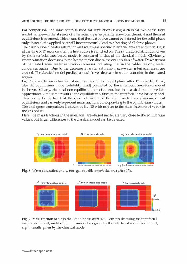
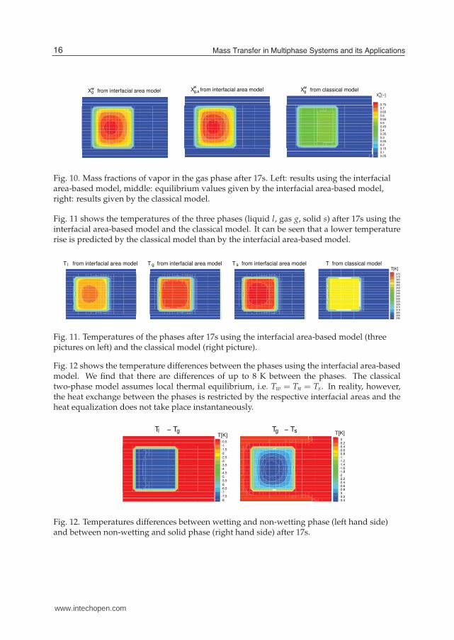
For comparison, the same setup is used for simulations using a classical two-phase flowmodel, where—in the absence of interfacial areas as parameters—local chemical and thermalequilibrium is assumed. This means that the heat source cannot be defined for the solid phaseonly; instead, the applied heat will instantaneously lead to a heating of all three phases.The distribution of water saturation and water–gas specific interfacial area are shown in Fig. 8at the time of 17 seconds after the heat source is switched on. The saturation distribution givenby the interfacial area-based model is compared to that of the classical model. Obviously,water saturation decreases in the heated region due to the evaporation of water. Downstreamof the heated zone, water saturation increases indicating that in the colder regions, watercondenses again. Due to the decrease in water saturation, gas–water interfacial areas arecreated. The classical model predicts a much lower decrease in water saturation in the heatedregion.Fig. 9 shows the mass fraction of air dissolved in the liquid phase after 17 seconds. There,also the equilibrium value (solubility limit) predicted by the interfacial area-based modelis shown. Clearly, chemical non-equilibrium effects occur, but the classical model predictsapproximately the same result as the equilibrium values in the interfacial area-based model.This is due to the fact that the classical two-phase flow approach always assumes localequilibrium and can only represent mass fractions corresponding to the equilibrium values.The analogous comparison is shown in Fig. 10 with respect to the mass fractions of vapor inthe gas phase.Here, the mass fractions in the interfacial area-based model are very close to the equilibriumvalues, but larger differences to the classical model can be detected.

Sw: 0.8 0.81 0.82 0.83 0.84 0.85 0.86 0.87 0.88 0.89 0.9 0.91 Sw: 0.8 0.81 0.82 0.83 0.84 0.85 0.86 0.87 0.88 0.89 0.9 0.91 awn: 380 400 420 440 460 480 500 520 540 560 580

S from interfacial area modell lS from classical model lga from interfacial area model

S a [1/m]l lg

Fig. 8. Water saturation and water–gas specific interfacial area after 17s.

Xsw2

2.36E-05

2.34E-052.32E-05

2.3E-05

2.28E-05

2.26E-05

2.24E-05

2.22E-05

2.2E-05

2.18E-05

2.16E-05

2.14E-05

lX from interfacial area modela

l,sX from interfacial area modela

la

X from classical model

2.36E.6

2.24E−6

X la

Fig. 9. Mass fraction of air in the liquid phase after 17s. Left: results using the interfacialarea-based model, middle: equilibrium values given by the interfacial area-based model,right: results given by the classical model.


www.intechopen.com

16 Mass Transfer

XWG

0.75

0.7

0.65

0.6

0.55

0.5

0.45

0.4

0.35

0.3

0.25

0.2

0.15

0.1

0.05

Xsn1

0.75

0.7

0.65

0.6

0.55

0.5

0.45

0.4

0.35

0.3

0.25

0.2

0.15

0.1

0.05

X from interfacial area modelw

gw

X from interfacial area model X from classical modelgw

g,sgX [−]w

Fig. 10. Mass fractions of vapor in the gas phase after 17s. Left: results using the interfacialarea-based model, middle: equilibrium values given by the interfacial area-based model,right: results given by the classical model.

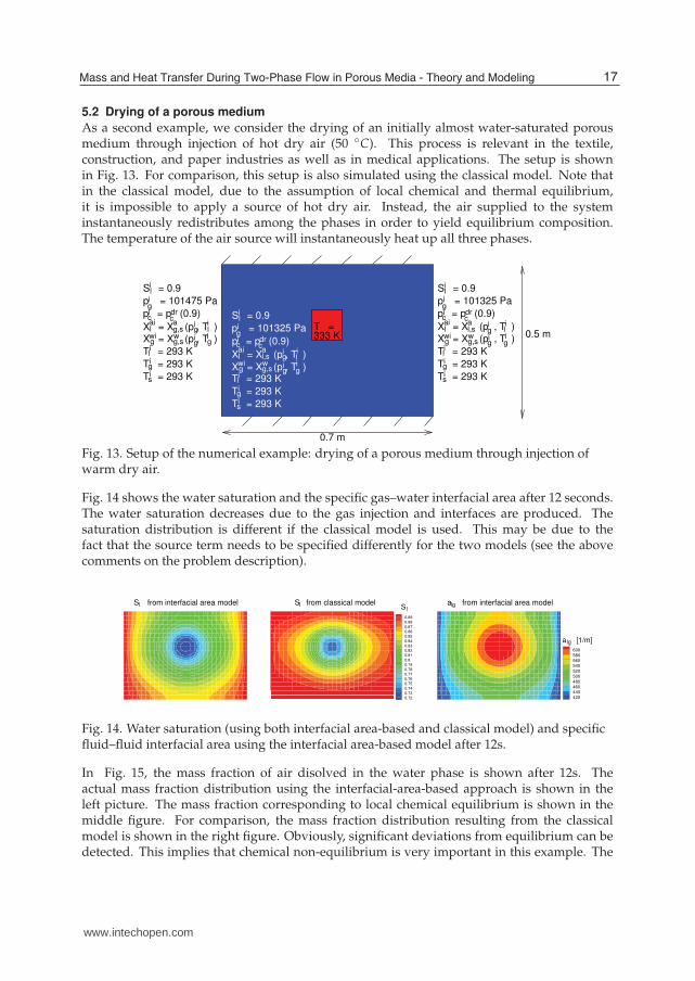
Fig. 11 shows the temperatures of the three phases (liquid l, gas g, solid s) after 17s using theinterfacial area-based model and the classical model. It can be seen that a lower temperaturerise is predicted by the classical model than by the interfacial area-based model.

Tn

375370365360355350345340335330325320315310305300295

Te

375370365360355350345340335330325320315310305300295

lT from interfacial area model gT from interfacial area model sT from interfacial area model T from classical modelT[K]

Fig. 11. Temperatures of the phases after 17s using the interfacial area-based model (threepictures on left) and the classical model (right picture).

Fig. 12 shows the temperature differences between the phases using the interfacial area-basedmodel. We find that there are differences of up to 8 K between the phases. The classicaltwo-phase model assumes local thermal equilibrium, i.e. Tw = Tn = Ts. In reality, however,the heat exchange between the phases is restricted by the respective interfacial areas and theheat equalization does not take place instantaneously.

dTnTs

0-0.2-0.4-0.6-0.8-1-1.2-1.4-1.6-1.8-2-2.2-2.4-2.6-2.8-3-3.2-3.4

dTwTn

-0.5

-1

-1.5

-2

-2.5

-3

-3.5

-4

-4.5

-5

-5.5

-6

-6.5

-7

-7.5

-8

T − Tl g T − Tg sT[K] T[K]

Fig. 12. Temperatures differences between wetting and non-wetting phase (left hand side)and between non-wetting and solid phase (right hand side) after 17s.


www.intechopen.com


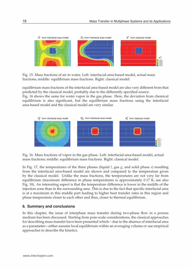
5.2 Drying of a porous medium

As a second example, we consider the drying of an initially almost water-saturated porousmedium through injection of hot dry air (50 ◦C). This process is relevant in the textile,construction, and paper industries as well as in medical applications. The setup is shownin Fig. 13. For comparison, this setup is also simulated using the classical model. Note thatin the classical model, due to the assumption of local chemical and thermal equilibrium,it is impossible to apply a source of hot dry air. Instead, the air supplied to the systeminstantaneously redistributes among the phases in order to yield equilibrium composition.The temperature of the air source will instantaneously heat up all three phases.

Qna

S = 0.9

p = 101475 Pa

T = 293 K

T = 293 K

T = 293 K

p = p (0.9)

s

g

l

gwl

c

g

l

ai ac

g,sw

i

i

i

i

i

i

i

g,s

dr

igigX = X (p , T )g

lX = X (p , T )

0.7 m

0.5 m

S = 0.9

p = 101325 Pa

X = X (p , T )

T = 293 K

T = 293 K

T = 293 K

p = p (0.9)

s

g

l

gwl

c

g

l

ai ac

g,sw

i

i

i

i

i

i

i

l,s

dr

i

ig

g

g

l333 KT =

ai

lS = 0.9i

p = 101325 Pai

cdr

c

wi

a

gT = 293 K

iT = 293 Kg

T = 293 K

wgi

ig

il

is

gip = p (0.9)

l l,s lX = X (p , T )

g g,sX = X (p , T )

i

i

i

iX = X (p , T )

i

i

Fig. 13. Setup of the numerical example: drying of a porous medium through injection ofwarm dry air.

Fig. 14 shows the water saturation and the specific gas–water interfacial area after 12 seconds.The water saturation decreases due to the gas injection and interfaces are produced. Thesaturation distribution is different if the classical model is used. This may be due to thefact that the source term needs to be specified differently for the two models (see the abovecomments on the problem description).

Sw

0.89

0.88

0.87

0.86

0.85

0.84

0.83

0.82

0.81

0.8

0.79

0.78

0.77

0.76

0.75

0.74

0.73

0.72

awn

600

580

560

540

520

500

480

460

440

420

Sw

0.89

0.88

0.87

0.86

0.85

0.84

0.83

0.82

0.81

0.8

0.79

0.78

0.77

0.76

0.75

0.74

0.73

0.72

S from interfacial area modell S from classical modell a from interfacial area modellgS

a [1/m]

l

lg

Fig. 14. Water saturation (using both interfacial area-based and classical model) and specificfluid–fluid interfacial area using the interfacial area-based model after 12s.

In Fig. 15, the mass fraction of air disolved in the water phase is shown after 12s. Theactual mass fraction distribution using the interfacial-area-based approach is shown in theleft picture. The mass fraction corresponding to local chemical equilibrium is shown in themiddle figure. For comparison, the mass fraction distribution resulting from the classicalmodel is shown in the right figure. Obviously, significant deviations from equilibrium can bedetected. This implies that chemical non-equilibrium is very important in this example. The


www.intechopen.com

18 Mass Transfer

XAW

2.348E-052.347E-052.346E-052.345E-052.344E-052.343E-052.342E-052.341E-05

XAW

2.348E-052.347E-052.346E-052.345E-052.344E-052.343E-052.342E-052.341E-05

X from interfacial area modelal X from classical modell

aX from interfacial area modell,s

a

X la

Fig. 15. Mass fractions of air in water. Left: interfacial-area-based model, actual massfractions; middle: equilibrium mass fractions. Right: classical model.

equilibrium mass fractions of the interfacial area-based model are also very different from thatpredicted by the classical model, probably due to the differently specified source.Fig. 16 shows the same for water vapor in the gas phase. Here, the deviation from chemicalequilibrium is also significant, but the equilibrium mass fractions using the interfacialarea-based model and the classical model are very similar.

XWG

0.01750.0170.01650.0160.01550.015

XWG

0.01750.0170.01650.0160.01550.015

X from interfacial area modelwg X from interfacial area modelg,s

wX from classical modelg

w

gX [−]w

Fig. 16. Mass fractions of vapor in the gas phase. Left: interfacial-area-based model, actualmass fractions; middle: equilibrium mass fractions. Right: classical model.

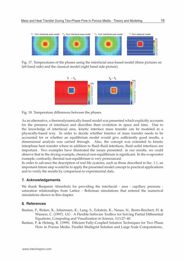
In Fig. 17, the temperatures of the three phases (liquid l, gas g, and solid phase s) resultingfrom the interfacial area-based model are shown and compared to the temperature givenby the classical model. Unlike the mass fractions, the temperatures are not very far fromequilibrium (maximum difference in phase temperatures is approximately 0.17 K, see alsoFig. 18). An interesting aspect is that the temperature difference is lower in the middle of theinjection zone than in the surrounding area. This is due to the fact that specific interfacial areais at a maximum in this middle part leading to higher heat transfer rates in this region andphase temperature closer to each other and thus, closer to thermal equilibrium.

6. Summary and conclusions

In this chapter, the issue of interphase mass transfer during two-phase flow in a porousmedium has been discussed. Starting from pore-scale considerations, the classical approachesfor describing mass transfer have been presented which—due to the absence of interfacial areaas a parameter—either assume local equilibrium within an averaging volume or use empiricalapproaches to describe the kinetics.


www.intechopen.com


Ts

296.4296.2296295.8295.6295.4295.2295294.8294.6294.4294.2294293.8293.6293.4293.2

Te

296.6296.4296.2296295.8295.6295.4295.2295294.8294.6294.4294.2294293.8293.6293.4

lT from interfacial area model gT from interfacial area model sT from interfacial area model T from classical model

T[K]

Fig. 17. Temperatures of the phases using the interfacial area-based model (three pictures onleft hand side) and the classical model (right hand side picture).

dTnTs

0.15

0.14

0.13

0.12

0.11

0.1

0.09

0.08

0.07

0.06

0.05

0.04

0.03

0.02

0.01

0

dTwTn

0-0.01-0.02-0.03-0.04-0.05-0.06-0.07-0.08-0.09-0.1-0.11-0.12-0.13-0.14-0.15-0.16-0.17

l g T − T g s T − T

T[K]

T[K]

Fig. 18. Temperature differences between the phases.

As an alternative, a thermodynamically-based model was presented which explicitly accountsfor the presence of interfaces and describes their evolution in space and time. Due tothe knowledge of interfacial area, kinetic interface mass transfer can be modeled in aphysically-based way. In order to decide whether kinetics of mass transfer needs to beaccounted for or whether an equilibrium model would give sufficiently good results, adimensional analysis was carried through. Also, the concept was extended to kineticinterphase heat transfer where in addition to fluid–fluid interfaces, fluid–solid interfaces areimportant. Two examples have illustrated the issues presented: in our results, we couldobserve that in the drying example, chemical non-equilibrium is significant. In the evaporatorexample, contrarily, thermal non-equilibrium is very pronounced.In order to advance the description of real life systems, such as those described in Sec. 1.1, animportant future step would be to apply the presented model concept to practical applicationsand to verify the results by comparison to experimental data.

7. Acknowledgements

We thank Benjamin Ahrenholz for providing the interfacial - area - capillary pressure -saturation relationships from Lattice - Boltzman simulations that entered the numericalsimulations shown in this chapter.

8. References

Bastian, P., Birken, K., Johannsen, K., Lang, S., Eckstein, K., Neuss, N., Rentz-Reichert, H. &Wieners, C. (1997). UG - A Flexible Software Toolbox for Solving Partial DifferentialEquations, Computing and Visualization in Science, 1(1):27–40.

Bastian, P. & Helmig, R. (1999). Efficient Fully-Coupled Solution Techniques for Two PhaseFlow in Porous Media. Parallel Multigrid Solution and Large Scale Computations.,


www.intechopen.com

20 Mass Transfer

Advances in Water Resources 23: 199–216.Bowen, R. (1982). Compressible Porous Media Models by Use of the Theory of Mixtures,

International Journal of Engineering Science 20(6): 697–735.Brusseau, M., Popovicova, J. & Silva, J. (1997). Characterizing gas–water interfacial

and bulk-water partitioning for gas phase transport of organic contaminants inunsaturated porous media, Environmental Sciences Technology 31: 1645–1649.

Chen, D., Pyrak-Nolte, L., Griffin, J. & Giordano, N. (2007). Measurement of interfacial areaper volume for drainage and imbibition, Water Resources Research 43(12).

Chen, L. & Kibbey, T. (2006). Measurement of air–water interfacial area for multiple hystereticdrainage curves in an unsaturated fine sand, Langmuir 22: 6674–6880.

Culligan, K., Wildenschild, D., Christensen, B., Gray, W., Rivers, M. & Tompson, A. (2004).Interfacial area measurements for unsaturated flow through a porous medium, WaterResources Research 40: 1–12.

Falta, R. W. (2000). Numerical modeling of kinetic interphase mass transfer during airsparging using a dual-media approach, Water Resources Research 36(12): 3391–3400.

Falta, R. W. (2003). Modeling sub-grid-block-scale dense nonaqueous phase liquid (DNAPL)pool dissolution using a dual-domain approach, Water Resources Research 39(12).

Gray, W. & Hassanizadeh, S. (1989). Averaging theorems and averaged equations for transportof interface properties in multiphase systems, International Journal of Multi-Phase Flow15: 81–95.

Gray, W. & Hassanizadeh, S. (1998). Macroscale continuum mechanics for multiphaseporous-media flow including phases, interfaces, common lines, and common points,Advances in Water Resources 21: 261–281.

Gray, W. & Miller, C. (2005). Thermodynamically Constrained Averaging Theory Approachfor Modeling of Flow in Porous Media: 1. Motivation and Overview, Advances inWater Resources 28(2): 161–180.

Hassanizadeh, S. M. & Gray, W. G. (1979). General Conservation Equations for Multi-PhaseSystems: 2. Mass, Momenta, Energy, and Entropy Equations, Advances in WaterResources 2: 191–203.

Hassanizadeh, S. M. & Gray, W. G. (1980). General Conservation Equations for Multi-PhaseSystems: 3. Constitutive Theory for Porous Media Flow, Advances in Water Resources3: 25–40.

Hassanizadeh, S. M. & Gray, W. G. (1990). Mechanics and Thermodynamics of MultiphaseFlow in Porous Media Including Interphase Boundaries, Advances in Water Resources13(4): 169–186.

Hassanizadeh, S. M. & Gray, W. G. (1993a). Thermodynamic Basis of Capillary Pressure inPorous Media, Water Resources Research 29(10): 3389 – 3405.

Hassanizadeh, S. M. & Gray, W. G. (1993b). Toward an improved description of the physics oftwo-phase flow, Advances in Water Resources 16(1): 53–67.

Held, R. & Celia, M. (2001). Modeling support of functional relationships between capillarypressure, saturation, interfacial area and common lines, Advances in Water Resources24: 325–343.

Imhoff, P., Jaffe, P. & Pinder, G. (1994). An experimental study of complete dissolutionof a nonaqueous phase liquid in saturated porous media, Water Resources Research30(2): 307–320.

IPCC (2005). Carbon Dioxide Capture and Storage. Special Report of the Intergovernmental Panel onClimate Change, Cambridge University Press.


www.intechopen.com


Jackson, A., Miller, C. & Gray, W. (2009). Thermodynamically constrained averaging theoryapproach for modeling flow and transport phenomena in porous medium systems:6. two-fluid-phase flow, Advances in Water Resources 32(6): 779–795.

Joekar-Niasar, V., Hassanizadeh, S. M. & Leijnse, A. (2008). Insights into the relationshipamong capillary pressure, saturation, interfacial area and relative permeability usingpore-scale network modeling, Transport in Porous Media 74: 201–219.

Joekar-Niasar, V., Hassanizadeh, S. M., Pyrak-Nolte, L. J. & Berentsen, C. (2009).Simulating drainage and imbibition experiments in a high-porosity micro-modelusing an unstructured pore-network model, Water Resources Research 45(W02430,doi:10.1029/2007WR006641).

Kalaydjian, F. (1987). A Macroscopic Description of Multiphase Flow in Porous MediaInvolving Spacetime Evolution of Fluid/Fluid Interface, Transport in Porous Media2: 537 – 552.

Ludecke, C. & Ludecke, D. (2000). Thermodynamik, Springer, Berlin.Marle, C.-M. (1981). From the pore scale to the macroscopic scale: Equations governing

multiphase fluid flow through porous media, Proceedings of Euromech 143, pp. 57–61.Delft, Verruijt, A. and Barends, F. B. J. (eds.).

Mayer, A. & Hassanizadeh, S. (2005). Soil and Groundwater Contamination: Nonaqueous PhaseLiquids, American Geophysical Union.

Miller, C., Poirier-McNeill, M. & Mayer, A. (1990). Dissolution of trapped nonaqueous phaseliquids: Mass transfer characteristics, Water Resources Research 21(2): 77–120.

Niessner, J. & Hassanizadeh, S. (2008). A Model for Two-Phase Flow in Porous MediaIncluding Fluid–Fluid Interfacial Area, Water Resources Research . 44, W08439,doi:10.1029/2007WR006721.

Niessner, J. & Hassanizadeh, S. (2009a). Modeling kinetic interphase mass transfer fortwo-phase flow in porous media including fluid–fluid interfacial area, Transport inPorous Media . doi:10.1007/s11242-009-9358-5.

Niessner, J. & Hassanizadeh, S. (2009b). Non-equilibrium interphase heat and mass transferduring two-phase flow in porous media—theoretical considerations and modeling,Advances in Water Resources 32: 1756–1766.

Porter, M., Schaap, M. & Wildenschild, D. (2009). Lattice-boltzmann simulations of thecapillary pressure-saturation-interfacial area relationship for porous media, Advancesin Water Resources 32(11): 1632–1640.

Powers, S., Abriola, L. & Weber, W. (1992). An experimental investigation of nonaqueousphase liquid dissolution in saturated subsurface systems: steady state mass transferrates, Water Resources Research 28: 2691–2706.

Powers, S., Abriola, L. & Weber, W. (1994). An experimental investigation of nonaqueousphase liquid dissolution in saturated subsurface systems: transient mass transferrates, Water Resources Research 30(2): 321–332.

Reeves, P. & Celia, M. (1996). A functional relationship between capillary pressure, saturation,and interfacial area as revealed by a pore-scale network model, Water ResourcesResearch 32(8): 2345–2358.

Schaefer, C., DiCarlo, D. & Blunt, M. (2000). Experimental measurements of air–waterinterfacial area during gravity drainage and secondary imbibition in porous media,Water Resources Research 36: 885–890.

van Antwerp, D., Falta, R. & Gierke, J. (2008). Numerical Simulation of Field-ScaleContaminant Mass Transfer during Air Sparging, Vadose Zone Journal 7: 294–304.


www.intechopen.com

22 Mass Transfer

Wildenschild, D., Hopmans, J., Vaz, C., Rivers, M. & Rikard, D. (2002). Using X-ray computedtomography in hydrology. Systems, resolutions, and limitations, Journal of Hydrology267: 285–297.

Zhang, H. & Schwartz, F. (2000). Simulating the in situ oxidative treatment of chlorinatedcompounds by potassium permanganate, Water Resources Research 36(10): 3031–3042.


www.intechopen.com

Mass Transfer in Multiphase Systems and its ApplicationsEdited by Prof. Mohamed El-Amin

ISBN 978-953-307-215-9Hard cover, 780 pagesPublisher InTechPublished online 11, February, 2011Published in print edition February, 2011

InTech EuropeUniversity Campus STeP Ri Slavka Krautzeka 83/A 51000 Rijeka, Croatia Phone: +385 (51) 770 447 Fax: +385 (51) 686 166www.intechopen.com

InTech ChinaUnit 405, Office Block, Hotel Equatorial Shanghai No.65, Yan An Road (West), Shanghai, 200040, China

Phone: +86-21-62489820 Fax: +86-21-62489821

This book covers a number of developing topics in mass transfer processes in multiphase systems for avariety of applications. The book effectively blends theoretical, numerical, modeling and experimental aspectsof mass transfer in multiphase systems that are usually encountered in many research areas such aschemical, reactor, environmental and petroleum engineering. From biological and chemical reactors to paperand wood industry and all the way to thin film, the 31 chapters of this book serve as an important reference forany researcher or engineer working in the field of mass transfer and related topics.

How to referenceIn order to correctly reference this scholarly work, feel free to copy and paste the following:

Jennifer Niessner and S. Majid Hassanizadeh (2011). Mass and Heat Transfer During Two-Phase Flow inPorous Media - Theory and Modeling, Mass Transfer in Multiphase Systems and its Applications, Prof.Mohamed El-Amin (Ed.), ISBN: 978-953-307-215-9, InTech, Available from:http://www.intechopen.com/books/mass-transfer-in-multiphase-systems-and-its-applications/mass-and-heat-transfer-during-two-phase-flow-in-porous-media-theory-and-modeling

Documents

Mass and Heat Transfer During Two-Phase Flow in …cdn.intechweb.org/pdfs/13526.pdfMass and Heat Transfer During Two-Phase Flow in Porous Media - Theory and Modeling 3 (a) Carbon capture