Embed Size (px)
Citation preview

i
MAS3314/8314:Multivariate Data Analysis
Prof D J Wilkinson
Module description:
In the 21st Century, statisticians and data analysts typically work with data sets containinga large number of observations and many variables. This course will consider methodsfor making sense of data of this kind, with an emphasis on practical techniques. Consider,for example, a medical database containing records on a large number of people. Eachperson has a height, a weight, an age, a blood type, a blood pressure, and a host ofother attributes, some quantitative, and others categorical. We will look at graphical anddescriptive techniques which help us to visualise a multi-dimensional data set and atinferential methods which help us to answer more specific questions about the populationfrom which the individuals were sampled. We will also consider new problems whicharise in the analysis of large and/or multi-dimensional data, such as variable selectionand multiple testing.
Course texts:
T. Hastie, R. Tibshirani, J. Friedman: The Elements of Statistical Learning: Data mining,inference, and prediction, 2nd Edition (Springer-Verlag, 2009).
B. Everitt: An R and S-Plus Companion to Multivariate Analysis (Springer-Verlag, 2005).
I will refer frequently to these texts in the notes, especially the former, which I will citeas [HTF]. I will refer to the latter as [Everitt], mainly for R-related information. Note thatthe PDF of the full text of [HTF] is available freely on-line, and that [Everitt] should beavailable electronically to Newcastle University students via the University Library readinglist web site.
WWW page:
http://www.staff.ncl.ac.uk/d.j.wilkinson/teaching/mas3314/
Last update:
May 29, 2012These notes correspond roughly to the course as delivered in the Spring of 2012. They
will be revised before I deliver the course again in the first half of 2013.Use the date above to check when this file was generated.
c© 2012, Darren J Wilkinson

Contents
1 Introduction to multivariate data 11.1 Introduction . . . . . . . . . . . . . . . . . . . . . . . . . . . . . . . . . . . . 1
1.1.1 A few quotes... . . . . . . . . . . . . . . . . . . . . . . . . . . . . . . 11.1.2 Data in the internet age . . . . . . . . . . . . . . . . . . . . . . . . . 21.1.3 Module outline . . . . . . . . . . . . . . . . . . . . . . . . . . . . . . 3
1.2 Multivariate data and basic visualisation . . . . . . . . . . . . . . . . . . . . 31.2.1 Tables . . . . . . . . . . . . . . . . . . . . . . . . . . . . . . . . . . . 31.2.2 Working with data frames . . . . . . . . . . . . . . . . . . . . . . . . 5
1.3 Representing and summarising multivariate data . . . . . . . . . . . . . . . 151.3.1 The sample mean . . . . . . . . . . . . . . . . . . . . . . . . . . . . 161.3.2 Sample variance and covariance . . . . . . . . . . . . . . . . . . . . 181.3.3 Sample correlation . . . . . . . . . . . . . . . . . . . . . . . . . . . . 27
1.4 Multivariate random quantities . . . . . . . . . . . . . . . . . . . . . . . . . 301.5 Transformation and manipulation of multivariate random quantities and data 31
1.5.1 Linear and affine transformations . . . . . . . . . . . . . . . . . . . . 321.5.2 Transforming multivariate random quantities . . . . . . . . . . . . . . 331.5.3 Transforming multivariate data . . . . . . . . . . . . . . . . . . . . . 37
2 PCA and matrix factorisations 442.1 Introduction . . . . . . . . . . . . . . . . . . . . . . . . . . . . . . . . . . . . 44
2.1.1 Factorisation, inversion and linear systems . . . . . . . . . . . . . . 442.2 Triangular matrices . . . . . . . . . . . . . . . . . . . . . . . . . . . . . . . . 45
2.2.1 Upper and lower triangular matrices . . . . . . . . . . . . . . . . . . 452.2.2 Unit triangular matrices . . . . . . . . . . . . . . . . . . . . . . . . . 462.2.3 Forward and backward substitution . . . . . . . . . . . . . . . . . . . 47
2.3 Triangular matrix decompositions . . . . . . . . . . . . . . . . . . . . . . . . 502.3.1 LU decomposition . . . . . . . . . . . . . . . . . . . . . . . . . . . . 502.3.2 LDMT decomposition . . . . . . . . . . . . . . . . . . . . . . . . . . . 522.3.3 LDLT decomposition . . . . . . . . . . . . . . . . . . . . . . . . . . . 522.3.4 The Cholesky decomposition . . . . . . . . . . . . . . . . . . . . . . 53
2.4 Other matrix factorisations . . . . . . . . . . . . . . . . . . . . . . . . . . . . 592.4.1 QR factorisation . . . . . . . . . . . . . . . . . . . . . . . . . . . . . 592.4.2 Least squares problems . . . . . . . . . . . . . . . . . . . . . . . . . 622.4.3 Spectral decomposition . . . . . . . . . . . . . . . . . . . . . . . . . 632.4.4 Mahalanobis transformation and distance . . . . . . . . . . . . . . . 662.4.5 The singular value decomposition (SVD) . . . . . . . . . . . . . . . . 71
2.5 Principal components analysis (PCA) . . . . . . . . . . . . . . . . . . . . . 73
ii

CONTENTS iii
2.5.1 Derivation from the spectral decomposition . . . . . . . . . . . . . . 732.5.2 Total variation and variance explained . . . . . . . . . . . . . . . . . 752.5.3 Principal components from a sample variance matrix . . . . . . . . . 762.5.4 Construction from the SVD . . . . . . . . . . . . . . . . . . . . . . . 79
2.6 Conclusion . . . . . . . . . . . . . . . . . . . . . . . . . . . . . . . . . . . . 83
3 Inference, the MVN and multivariate regression 843.1 Inference and estimation . . . . . . . . . . . . . . . . . . . . . . . . . . . . . 843.2 Multivariate regression . . . . . . . . . . . . . . . . . . . . . . . . . . . . . . 87
3.2.1 Univariate multiple linear regression . . . . . . . . . . . . . . . . . . 883.2.2 The general linear model . . . . . . . . . . . . . . . . . . . . . . . . 913.2.3 Weighted errors . . . . . . . . . . . . . . . . . . . . . . . . . . . . . 93
3.3 The multivariate normal (MVN) distribution . . . . . . . . . . . . . . . . . . . 943.3.1 Evaluation of the MVN density . . . . . . . . . . . . . . . . . . . . . 953.3.2 Properties of the MVN . . . . . . . . . . . . . . . . . . . . . . . . . . 963.3.3 Maximum likelihood estimation . . . . . . . . . . . . . . . . . . . . . 983.3.4 MLE for the general linear model . . . . . . . . . . . . . . . . . . . . 100
4 Cluster analysis and unsupervised learning 1024.1 Introduction . . . . . . . . . . . . . . . . . . . . . . . . . . . . . . . . . . . . 102
4.1.1 Motivation . . . . . . . . . . . . . . . . . . . . . . . . . . . . . . . . . 1024.1.2 Dissimilarity and distance . . . . . . . . . . . . . . . . . . . . . . . . 102
4.2 Clustering methods . . . . . . . . . . . . . . . . . . . . . . . . . . . . . . . . 1044.2.1 K-means clustering . . . . . . . . . . . . . . . . . . . . . . . . . . . 1044.2.2 Hierarchical clustering . . . . . . . . . . . . . . . . . . . . . . . . . . 1124.2.3 Model-based clustering . . . . . . . . . . . . . . . . . . . . . . . . . 122
5 Discrimination and classification 1235.1 Introduction . . . . . . . . . . . . . . . . . . . . . . . . . . . . . . . . . . . . 1235.2 Heuristic classifiers . . . . . . . . . . . . . . . . . . . . . . . . . . . . . . . . 123
5.2.1 Closest group mean classifier . . . . . . . . . . . . . . . . . . . . . . 1235.2.2 Linear discriminant analysis (LDA) . . . . . . . . . . . . . . . . . . . 1255.2.3 Quadratic discrimination . . . . . . . . . . . . . . . . . . . . . . . . . 1275.2.4 Discrimination functions . . . . . . . . . . . . . . . . . . . . . . . . . 128
5.3 Maximum likelihood discrimination . . . . . . . . . . . . . . . . . . . . . . . 1295.3.1 LDA . . . . . . . . . . . . . . . . . . . . . . . . . . . . . . . . . . . . 1295.3.2 Quadratic discriminant analysis (QDA) . . . . . . . . . . . . . . . . . 1305.3.3 Estimation from data . . . . . . . . . . . . . . . . . . . . . . . . . . . 131
5.4 Misclassification . . . . . . . . . . . . . . . . . . . . . . . . . . . . . . . . . 1335.5 Bayesian classification . . . . . . . . . . . . . . . . . . . . . . . . . . . . . . 136
6 Graphical modelling 1386.1 Introduction . . . . . . . . . . . . . . . . . . . . . . . . . . . . . . . . . . . . 1386.2 Independence, conditional independence and factorisation . . . . . . . . . 1386.3 Undirected graphs . . . . . . . . . . . . . . . . . . . . . . . . . . . . . . . . 141
6.3.1 Graph theory . . . . . . . . . . . . . . . . . . . . . . . . . . . . . . . 1416.3.2 Graphical models . . . . . . . . . . . . . . . . . . . . . . . . . . . . . 143
6.4 Gaussian graphical models (GGMs) . . . . . . . . . . . . . . . . . . . . . . 145
CONTENTS iv
6.4.1 Partial covariance and correlation . . . . . . . . . . . . . . . . . . . 1476.5 Directed acyclic graph (DAG) models . . . . . . . . . . . . . . . . . . . . . . 152
6.5.1 Introduction . . . . . . . . . . . . . . . . . . . . . . . . . . . . . . . . 1526.5.2 Directed graphs . . . . . . . . . . . . . . . . . . . . . . . . . . . . . 1526.5.3 DAG models . . . . . . . . . . . . . . . . . . . . . . . . . . . . . . . 1536.5.4 Fitting to data . . . . . . . . . . . . . . . . . . . . . . . . . . . . . . . 158
6.6 Conclusion . . . . . . . . . . . . . . . . . . . . . . . . . . . . . . . . . . . . 159
7 Variable selection and multiple testing 1607.1 Regularisation and variable selection . . . . . . . . . . . . . . . . . . . . . . 160
7.1.1 Introduction . . . . . . . . . . . . . . . . . . . . . . . . . . . . . . . . 1607.1.2 Ridge regression . . . . . . . . . . . . . . . . . . . . . . . . . . . . . 1617.1.3 The LASSO and variable selection . . . . . . . . . . . . . . . . . . . 1647.1.4 The elastic net . . . . . . . . . . . . . . . . . . . . . . . . . . . . . . 1667.1.5 p >> n . . . . . . . . . . . . . . . . . . . . . . . . . . . . . . . . . . 167
7.2 Multiple testing . . . . . . . . . . . . . . . . . . . . . . . . . . . . . . . . . . 1687.2.1 Introduction . . . . . . . . . . . . . . . . . . . . . . . . . . . . . . . . 1687.2.2 The multiple testing problem . . . . . . . . . . . . . . . . . . . . . . 1697.2.3 Bonferroni correction . . . . . . . . . . . . . . . . . . . . . . . . . . . 1697.2.4 False discovery rate (FDR) . . . . . . . . . . . . . . . . . . . . . . . 170
Chapter 1
Introduction to multivariate data andrandom quantities
1.1 Introduction
1.1.1 A few quotes...
Google’s Chief Economist Hal Varian on Statistics and Data:
I keep saying the sexy job in the next ten years will be statisticians. Peoplethink I’m joking, but who would’ve guessed that computer engineers would’vebeen the sexy job of the 1990s?
Varian then goes on to say:
The ability to take data - to be able to understand it, to process it, to extractvalue from it, to visualize it, to communicate it’s going to be a hugely importantskill in the next decades, not only at the professional level but even at theeducational level for elementary school kids, for high school kids, for collegekids. Because now we really do have essentially free and ubiquitous data.So the complimentary scarce factor is the ability to understand that data andextract value from it.
Source: FlowingData.com
The big data revolution’s “lovely” and “lousy” jobs:
The lovely jobs are why we should all enroll our children immediately in statis-tics courses. Big data can only be unlocked by shamans with tremendousmathematical aptitude and training. McKinsey estimates that by 2018 in theUnited States alone, there will be a shortfall of between 140,000 and 190,000graduates with “deep analytical talent”. If you are one of them, you will surelyhave a “lovely” well-paying job.
Source: The Globe and Mail
1
CHAPTER 1. INTRODUCTION TO MULTIVARIATE DATA 2
The Search For Analysts To Make Sense Of ’Big Data’ (an article on an NPR programme)begins:
Businesses keep vast troves of data about things like online shopping behav-ior, or millions of changes in weather patterns, or trillions of financial transac-tions — information that goes by the generic name of big data.
Now, more companies are trying to make sense of what the data can tell themabout how to do business better. That, in turn, is fueling demand for peoplewho can make sense of the information — mathematicians — and creatingsomething of a recruiting war.
Source: NPR.org
Also see this article in the NYT: For Today’s Graduate, Just One Word: Statistics
1.1.2 Data in the internet age
It is clear from the above quotes and articles that technology is currently having a dra-matic impact on the way that data is being collected and analysed in the 21st Century.Until recently, the cost of collecting and measuring data for statistical analysis and in-terpretation meant that most analyses of statistical data concerned small data sets orcarefully designed experiments that were relatively straightforward to model. Today, mostorganisations (commercial businesses and companies, as well as other institutions, suchas research institutes and public sector bodies) record and conduct most aspects of theiroperation electronically, by default. Furthermore, technology for measuring, recording,analysing, and archiving data is rapidly evolving, and this is leading to a so-called “dataexplosion”. Most organisations have vast “data warehouses” of information which containvital information that could allow the organisation to work more effectively. The businessof extracting value from such data goes by various names in different contexts, including“business intelligence”, “business analytics”, “predictive analytics”, “predictive modelling”,“informatics”, “machine learning”, “data science”, “data mining”, as well as the more con-ventional “data analysis and modelling”. Occasionally, even as “statistics”...
Similarly, many areas of scientific research are currently being similarly transformed.Within physics, the CERN Large Hadron Collider is generating terabytes of data. In biol-ogy, new technologies such as high throughput sequencing are resulting in routine gener-ation of massive data sets. Here a typical (processed) datafile will contain many millions of“reads”, each of which will consist of around 100 base pairs (letters), and a typical exper-iment will generate several such data files. Such experiments are being conducted everyday in research institutions all over the world, and “bioinformaticians” skilled in statisticsand data analysis are in short supply.
Analysing and interpreting large and complex data sets is a significant challenge re-quiring many skills, including those of statistical data analysis and modelling. It would beunrealistic to attempt in a single module to provide all of the knowledge and skills neces-sary to become a real “data scientist”. Here we will concentrate on some of the key statis-tical concepts and techniques necessary for modern data analysis. Typical characteristicsof modern data analysis include working with data sets that are large, multivariate, andhighly structured, but with a non-trivial structure inconsistent with classical experimentaldesign ideas.
CHAPTER 1. INTRODUCTION TO MULTIVARIATE DATA 3
1.1.3 Module outline
Chapter 1: Introduction to multivariate data and random quantitiesThis first chapter will lay the foundation for the rest of the course, providing an intro-duction to multivariate data, mainly using R “data frames” as a canonical example,and introducing some basic methods for visualisation and summarisation, illustratedwith plenty of worked examples.
Chapter 2: PCA and matrix factorisationsIn this chapter we will examine how techniques from linear algebra can be used totransform data in a way that better reveals its underlying structure, and the role thatmatrix factorisations play in this. Principal components analysis (PCA) will be usedto illustrate the ideas.
Chapter 3: Inference, the MVN distribution, and multivariate regressionIn this chapter we will introduce the simplest and most useful multivariate probabilitydistribution: the multivariate normal (MVN) distribution. We will construct it, exam-ine some of its key properties, and look at some applications. We will also brieflyexamine linear regression for multivariate outputs.
Chapter 4: Cluster analysis and unsupervised learningIn this chapter we will look at how it is possible to uncover latent structure in multi-variate data without any “training data”. Clustering is the canonical example of whatdata miners refer to as “unsupervised learning”.
Chapter 5: Discrimination and classificationIn this chapter we will briefly examine the related problems of discrimination andclassification.
Chapter 6: Graphical modellingIn this chapter we will look how notions of conditional independence can be usedto understand multivariate relationships, and how these naturally lead to graphicalmodels of variable dependencies.
Chapter 7: Variable selection and multiple testingIn this final chapter we will look briefly at some of the issues that arise when workingwith data sets that are large or high dimensional.
1.2 Multivariate data and basic visualisation
1.2.1 Tables
Many interesting data sets start life as a (view of a) table from a relational database. Notat all coincidentally, database tables have a structure very similar to an R “data frame” (Rdata frames are modelled on relational database tables). Therefore for this course we willrestrict our attention to the analysis and interpretation of data sets contained in R dataframes. Conceptually a data frame consists as a collection of n “rows”, each of which is ap-tuple, xi = (xi1, xi2, . . . , xip) from some set of the form S1 × S2 × · · · × Sp, where each Sjis typically a finite discrete set (representing a factor ) or Sj ⊆ R. In the important special

CHAPTER 1. INTRODUCTION TO MULTIVARIATE DATA 4
case where we have Sj ⊆ R, j = 1, 2, . . . , p, we may embed each Sj in R and regardeach p-tuple xi as a vector in (some subset of) Rp. If we now imagine our collection ofp-tuples stacked one on top of the other, we have a table with n rows and p columns,where everything in the jth column is an element of Sj. In fact, R internally stores dataframes as a list of columns of the same length, where everything in the column is a vectorof a particular type.∗ It is important to make a clear distinction between the rows andthe columns. The rows, i = 1, . . . , n typically represent cases, or individuals, or items,or objects, or replicates, or observations, or realisations (from a probability model). Thecolumns j = 1, . . . , p represent attributes, or variables, or types, or factors associated witha particular case, and each contains data that are necessarily of the same type.
Example: Insect sprays
To make things concrete, let’s look at a few simple data frames bundled as standarddata frames in R. We can get a list of R data sets using the R command data(). Thedata set InsectSprays is a data frame. We can get information about this object with?InsectSprays, and we can look at the first few rows with> head(InsectSprays)
count spray1 10 A2 7 A3 20 A4 14 A5 14 A6 12 A>
The data represents counts of numbers of insects in a given agricultural area for differentkinds of insect sprays. We can get a simple plot of the data with boxplot(count∼spray,data=InsectSprays) (which shows that sprays C, D and E seem to be most effective),and understand the content with> class(InsectSprays)[1] "data.frame"> dim(InsectSprays)[1] 72 2> levels(InsectSprays$spray)[1] "A" "B" "C" "D" "E" "F"> table(InsectSprays$count)
0 1 2 3 4 5 6 7 9 10 11 12 13 14 15 16 17 19 20 21 22 23 24 262 6 4 8 4 7 3 3 1 3 3 2 4 4 2 2 4 1 2 2 1 1 1 2> str(InsectSprays)’data.frame’: 72 obs. of 2 variables:$ count: num 10 7 20 14 14 12 10 23 17 20 ...$ spray: Factor w/ 6 levels "A","B","C","D",..: 1 1 1 1 1 1 1 1 1 1
...
∗This internal storage is different to the way that relational databases typically store tables — database tables aretypically stored internally as collections of rows. However, since R provides mechanisms for accessing data by rowsas well as columns, this difference will not trouble us.
CHAPTER 1. INTRODUCTION TO MULTIVARIATE DATA 5
>
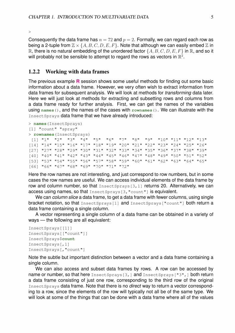
Consequently the data frame has n = 72 and p = 2. Formally, we can regard each row asbeing a 2-tuple from Z× {A,B,C,D,E, F}. Note that although we can easily embed Z inR, there is no natural embedding of the unordered factor {A,B,C,D,E, F} in R, and so itwill probably not be sensible to attempt to regard the rows as vectors in R2.
1.2.2 Working with data frames
The previous example R session shows some useful methods for finding out some basicinformation about a data frame. However, we very often wish to extract information fromdata frames for subsequent analysis. We will look at methods for transforming data later.Here we will just look at methods for extracting and subsetting rows and columns froma data frame ready for further analysis. First, we can get the names of the variablesusing names(), and the names of the cases with rownames(). We can illustrate with theInsectSprays data frame that we have already introduced:
> names(InsectSprays)[1] "count" "spray"> rownames(InsectSprays)[1] "1" "2" "3" "4" "5" "6" "7" "8" "9" "10" "11" "12" "13"[14] "14" "15" "16" "17" "18" "19" "20" "21" "22" "23" "24" "25" "26"[27] "27" "28" "29" "30" "31" "32" "33" "34" "35" "36" "37" "38" "39"[40] "40" "41" "42" "43" "44" "45" "46" "47" "48" "49" "50" "51" "52"[53] "53" "54" "55" "56" "57" "58" "59" "60" "61" "62" "63" "64" "65"[66] "66" "67" "68" "69" "70" "71" "72"
Here the row names are not interesting, and just correspond to row numbers, but in somecases the row names are useful. We can access individual elements of the data frame byrow and column number, so that InsectSprays[3,1] returns 20. Alternatively, we canaccess using names, so that InsectSprays[3,"count"] is equivalent.
We can column slice a data frame, to get a data frame with fewer columns, using singlebracket notation, so that InsectSprays[1] and InsectSprays["count"] both return adata frame containing a single column.
A vector representing a single column of a data frame can be obtained in a variety ofways — the following are all equivalent:
InsectSprays[[1]]InsectSprays[["count"]]InsectSprays$countInsectSprays[,1]InsectSprays[,"count"]
Note the subtle but important distinction between a vector and a data frame containing asingle column.
We can also access and subset data frames by rows. A row can be accessed byname or number, so that here InsectSprays[3,] and InsectSprays["3",] both returna data frame consisting of just one row, corresponding to the third row of the originalInsectSprays data frame. Note that there is no direct way to return a vector correspond-ing to a row, since the elements of the row will typically not all be of the same type. Wewill look at some of the things that can be done with a data frame where all of the values

CHAPTER 1. INTRODUCTION TO MULTIVARIATE DATA 6
are numeric in the next example. We can create a data frame containing a subset of rowsfrom the data frame by using a vector of row numbers or names. eg.
> InsectSprays[3:5,]count spray
3 20 A4 14 A5 14 A>
We can also subset the rows using a boolean vector of length n which has TRUE elementscorresponding the the required rows. eg. InsectSprays[InsectSprays$spray=="B",]will extract the rows where the spray factor is B. If the vector of counts is required, thiscan be extracted from the resulting data frame in the usual way, but this could also beobtained more directly using
> InsectSprays$count[InsectSprays$spray=="B"][1] 11 17 21 11 16 14 17 17 19 21 7 13
>
Example: Motor Trend Cars
We will illustrate a few more important R techniques for working with data frames usinganother simple built-in data set, mtcars, before moving on to look at some more interest-ing examples. Again, the str() command is very useful.
> str(mtcars)’data.frame’: 32 obs. of 11 variables:$ mpg : num 21 21 22.8 21.4 18.7 18.1 14.3 24.4 22.8 19.2 ...$ cyl : num 6 6 4 6 8 6 8 4 4 6 ...$ disp: num 160 160 108 258 360 ...$ hp : num 110 110 93 110 175 105 245 62 95 123 ...$ drat: num 3.9 3.9 3.85 3.08 3.15 2.76 3.21 3.69 3.92 3.92 ...$ wt : num 2.62 2.88 2.32 3.21 3.44 ...$ qsec: num 16.5 17 18.6 19.4 17 ...$ vs : num 0 0 1 1 0 1 0 1 1 1 ...$ am : num 1 1 1 0 0 0 0 0 0 0 ...$ gear: num 4 4 4 3 3 3 3 4 4 4 ...$ carb: num 4 4 1 1 2 1 4 2 2 4 ...
>
So we see that we have n = 32 and p = 11, and here also that all 11 variables are numeric, so we could regard the rows as points in R11 if we felt that was sensible. However, closerinspection reveals that some columns are counts, and some are numeric encodings ofbinary variables, so direct embedding into R11 may not be such a great idea. This dataframe has sensible names for both the rows and the columns
> names(mtcars)[1] "mpg" "cyl" "disp" "hp" "drat" "wt" "qsec" "vs" "am" "
gear"[11] "carb"> rownames(mtcars)
CHAPTER 1. INTRODUCTION TO MULTIVARIATE DATA 7
[1] "Mazda RX4" "Mazda RX4 Wag" "Datsun 710"[4] "Hornet 4 Drive" "Hornet Sportabout" "Valiant"[7] "Duster 360" "Merc 240D" "Merc 230"
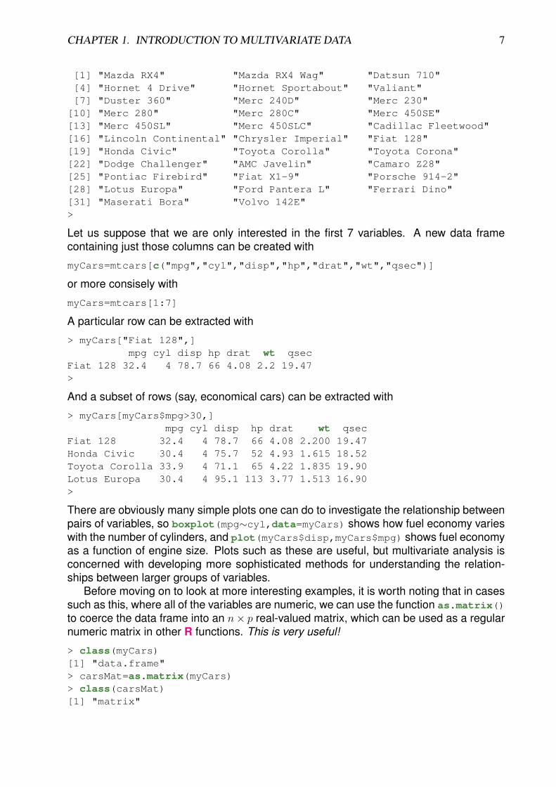
[10] "Merc 280" "Merc 280C" "Merc 450SE"[13] "Merc 450SL" "Merc 450SLC" "Cadillac Fleetwood"[16] "Lincoln Continental" "Chrysler Imperial" "Fiat 128"[19] "Honda Civic" "Toyota Corolla" "Toyota Corona"[22] "Dodge Challenger" "AMC Javelin" "Camaro Z28"[25] "Pontiac Firebird" "Fiat X1-9" "Porsche 914-2"[28] "Lotus Europa" "Ford Pantera L" "Ferrari Dino"[31] "Maserati Bora" "Volvo 142E">
Let us suppose that we are only interested in the first 7 variables. A new data framecontaining just those columns can be created with
myCars=mtcars[c("mpg","cyl","disp","hp","drat","wt","qsec")]
or more consisely with
myCars=mtcars[1:7]
A particular row can be extracted with
> myCars["Fiat 128",]mpg cyl disp hp drat wt qsec
Fiat 128 32.4 4 78.7 66 4.08 2.2 19.47>
And a subset of rows (say, economical cars) can be extracted with
> myCars[myCars$mpg>30,]mpg cyl disp hp drat wt qsec
Fiat 128 32.4 4 78.7 66 4.08 2.200 19.47Honda Civic 30.4 4 75.7 52 4.93 1.615 18.52Toyota Corolla 33.9 4 71.1 65 4.22 1.835 19.90Lotus Europa 30.4 4 95.1 113 3.77 1.513 16.90>
There are obviously many simple plots one can do to investigate the relationship betweenpairs of variables, so boxplot(mpg∼cyl,data=myCars) shows how fuel economy varieswith the number of cylinders, and plot(myCars$disp,myCars$mpg) shows fuel economyas a function of engine size. Plots such as these are useful, but multivariate analysis isconcerned with developing more sophisticated methods for understanding the relation-ships between larger groups of variables.
Before moving on to look at more interesting examples, it is worth noting that in casessuch as this, where all of the variables are numeric, we can use the function as.matrix()to coerce the data frame into an n× p real-valued matrix, which can be used as a regularnumeric matrix in other R functions. This is very useful!
> class(myCars)[1] "data.frame"> carsMat=as.matrix(myCars)> class(carsMat)[1] "matrix"
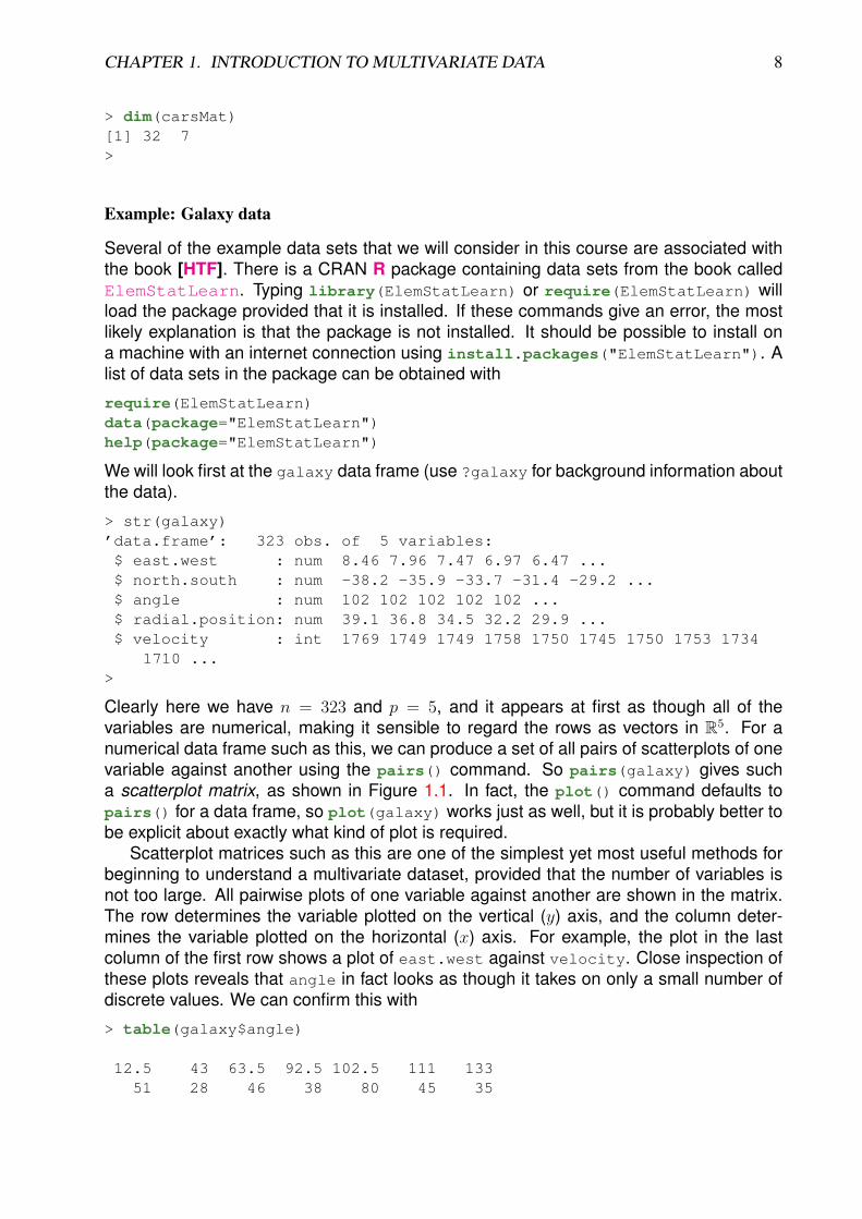
CHAPTER 1. INTRODUCTION TO MULTIVARIATE DATA 8
> dim(carsMat)[1] 32 7>
Example: Galaxy data
Several of the example data sets that we will consider in this course are associated withthe book [HTF]. There is a CRAN R package containing data sets from the book calledElemStatLearn. Typing library(ElemStatLearn) or require(ElemStatLearn) willload the package provided that it is installed. If these commands give an error, the mostlikely explanation is that the package is not installed. It should be possible to install ona machine with an internet connection using install.packages("ElemStatLearn"). Alist of data sets in the package can be obtained with
require(ElemStatLearn)data(package="ElemStatLearn")help(package="ElemStatLearn")
We will look first at the galaxy data frame (use ?galaxy for background information aboutthe data).
> str(galaxy)’data.frame’: 323 obs. of 5 variables:$ east.west : num 8.46 7.96 7.47 6.97 6.47 ...$ north.south : num -38.2 -35.9 -33.7 -31.4 -29.2 ...$ angle : num 102 102 102 102 102 ...$ radial.position: num 39.1 36.8 34.5 32.2 29.9 ...$ velocity : int 1769 1749 1749 1758 1750 1745 1750 1753 1734
1710 ...>
Clearly here we have n = 323 and p = 5, and it appears at first as though all of thevariables are numerical, making it sensible to regard the rows as vectors in R5. For anumerical data frame such as this, we can produce a set of all pairs of scatterplots of onevariable against another using the pairs() command. So pairs(galaxy) gives sucha scatterplot matrix, as shown in Figure 1.1. In fact, the plot() command defaults topairs() for a data frame, so plot(galaxy) works just as well, but it is probably better tobe explicit about exactly what kind of plot is required.
Scatterplot matrices such as this are one of the simplest yet most useful methods forbeginning to understand a multivariate dataset, provided that the number of variables isnot too large. All pairwise plots of one variable against another are shown in the matrix.The row determines the variable plotted on the vertical (y) axis, and the column deter-mines the variable plotted on the horizontal (x) axis. For example, the plot in the lastcolumn of the first row shows a plot of east.west against velocity. Close inspection ofthese plots reveals that angle in fact looks as though it takes on only a small number ofdiscrete values. We can confirm this with
> table(galaxy$angle)
12.5 43 63.5 92.5 102.5 111 13351 28 46 38 80 45 35

CHAPTER 1. INTRODUCTION TO MULTIVARIATE DATA 9
east.west
−40 0 40
●●●●●●●●●●●●●●●●●●●●●●●●●●●●●●●●●●●●●
●●●●●●●●●●●●●●●●●●●●●●●●
●●●●●●●●●●●●●●●●●●●●●●●●●●●●●●●●●●●
●●●●●●●●●●●●●●●●●●●●●●●●●●●●●●●●●●●●●●●●●●●●●
●●●●●●●●●●●●●●●●●●●●●●●●●●●●
●●●●●●●●●●●●●●●●●●●●●●●●●●●●●●●●●●●●●●
●●●●●●●●●●●●●●●●●●●●●●●●●●●●●●●●●●●●●●●●●●●●●●
●●●●●●●●●●●●●●●●●●●●●●●●●●●
●●●●●●●●●●●●●●●●●●●●●●●●●●●●●●●●●●●●●●●●●●●
−40 0 40
●●●●●●●●●●●●●●●●●●●●●●●●●●●●●●●●●●●●●
●●●●●●●●●●●●●●●●●●●●●●●●
●●●●●●●●●●●●●●●●●●●●●●●●●●●●●●●●●●●
●●●●●●●●●●●●●●●●●●●●●●●●●●●●●●●●●●●●●●●●●●●●●
●●●●●●●●●●●●●●●●●●●●●●●●●●●●
●●●●●●●●●●●●●●●●●●●●●●●●●●●●●●●●●●●●●●
●●●●●●●●●●●●●●●●●●●●●●●●●●●●●●●●●●●●●●●●●●●●●●
●●●●●●●●●●●●●●●●●●●●●●●●●●●
●●●●●●●●●●●●●●●●●●●●●●●●●●●●●●●●●●●●●●●●●●●
−30
10●●●●●●●●●●●●●●●●●●●●●●●●●●●●●●●●●●● ●●
●●●●●●●●● ●●●●●●●●●●●●●●●
●●●●●●●●●●●●●●●●●●●●●●●●●●●●●●●●●●●
●●●●●● ●●●●●●●●●●●●●●●●●●●●●●●●●●●●●●●●●●●●●●●
●●●●●●●●●●●●●●●●●●●● ●●●●● ●●●
●● ●●● ●●●●●●●●● ●●●●●●●●●●●●●●●●●●●●●●●●
●●●●●●●●●●●●●●●●●●●●●●●●● ●●●●●●●●●●●●●●●● ●●●●●
●●●●●●●●●●●●●●●●●●●●●●●●●●●
●● ●●●●●●●●●●●●●●●●●●●●●●●●●●●●●●●●●●●●●●●●●
−40
20
●●●●●●●●
●●●●●●●●
●●●●●●●●
●●●●●●●●
●●●●●
●●●●●●●●●●●●●●●●●●●●●●●●●●●●●
●●●●●●●●●●
●●●●●●●●●●
●●●●●●●●●●
●●●●●●●●
●●●●●●●●
●●●●●●●●
●●●●●●●●
●●●●●●●●
●●●●●
●●●●●●●●●●●●●●●●●●●●●●●●●●●●
●●●●●●●●●●●●●●●●●●●●●●●●●●●●●●●●●●●●●●
●●●●●●●●●●●●●●●●●●●●●●●●●●●●●●●●●●●●●●●●●●●●●●
●●●●●●●●●●●●●●●●●●●●●●●●●●●
●●●●●●
●●●●●●●●
●●●●●●●●
●●●●●●●●
●●●●●●●●
●●●●●
north.south●●●●●●●●●●●●●●●●●●●●●●●●●●●●●●●●●●●●●
●●●●●●●●●●●●●●●●●●●●●●●●●●●●●●●●●●●●●●●●●●●●●●●●●●●●●●●●●●●
●●●●●●●●●●●●●●●●●●●●●●●●●●●●●●●●●●●●●●●●●●●●●
●●●●●●●●●●●●●●●●●●●●●●●●●●●●
●●●●●●●●●●●●●●●●●●●●●●●●●●●●●●●●●●●●●●
●●●●●●●●●●●●●●●●●●●●●●●●●●●●●●●●●●●●●●●●●●●●●●
●●●●●●●●●●●●●●●●●●●●●●●●●●●
●●●●●●●●●●●●●●●●●●●●●●●●●●●●●●●●●●●●●●●●●●●
●●●●●●●●
●●●●●●●●
●●●●●●●●
●●●●●●●●
●●●●●
●●●●●●●●●●●●●●●●●●●●●●●●●●●●●
●●●●●●●●●●
●●●●●●●●●●
●●●●●●●●●●
●●●●●●●●
●●●●●●●●
●●●●●●●●
●●●●●●●●
●●●●●●●●
●●●●●
●●●●●●●●●●●●●●●●●●●●●●●●●●●●
●●●●●●●●●
●●●●●●●●
●●●●●●●●
●●●●●●●●
●●●●● ●●●●●●●●●●●●●●●●●●●●●●●●●●●●●●●●●●●●●●●●●●●●●●
●●●●●●●●●●●●●●●●●●●●●●●●●●●
●●●●●●●●●
●●●●●●●●
●●●●●●●●
●●●●●●●●
●●●●●●●●
●●
●●●●●●●●●●●●●●●●●●●●●●●●●●●
●●●●●●●● ●●
●●●●●●●●● ●●●●●●●●●●●●●●●●●●●●●●●●●●●●●●●●●●●●●●●●●
●●●●●●●●●
●●●●●● ●●●●
●●●●●●●●●●●●●●●●●●●●●●●
●●●●●●●●●●●●
●●●●●●●●●●●●●●●●●●●● ●●●●● ●●●
●● ●●● ●●●●●●●●● ●●●●●●●●●●●
●●●●●●●●●
●●●●●●●●●●●●●●●●●●●●●●●●●●●●● ●●●●●●●●●●●●●●●● ●●●●●
●●●●●●●●●●●●●●●●●●●●●●●●●●●
●● ●●●●●●●●●●
●●●●●●●●●●●●●●●●●●●●●●●●●●●●●●●
●●●●●●●●●●●●●●●●●●●●●●●●●●●●●●●●●●●●●
●●●●●●●●●●●●●●●●●●●●●●●●
●●●●●●●●●●●●●●●●●●●●●●●●●●●●●●●●●●●●●●●●●●●●●●●●●●●●●●●●●●●●●●●●●●●●●●●●●●●●●●●●
●●●●●●●●●●●●●●●●●●●●●●●●●●●●
●●●●●●●●●●●●●●●●●●●●●●●●●●●●●●●●●●●●●●
●●●●●●●●●●●●●●●●●●●●●●●●●●●●●●●●●●●●●●●●●●●●●●
●●●●●●●●●●●●●●●●●●●●●●●●●●●
●●●●●●●●●●●●●●●●●●●●●●●●●●●●●●●●●●●●●●●●●●● ●●●●●●●●●●●●●●●●●●●●●●●●●●●●●●●●●●●●●
●●●●●●●●●●●●●●●●●●●●●●●●
●●●●●●●●●●●●●●●●●●●●●●●●●●●●●●●●●●●●●●●●●●●●●●●●●●●●●●●●●●●●●●●●●●●●●●●●●●●●●●●●
●●●●●●●●●●●●●●●●●●●●●●●●●●●●
●●●●●●●●●●●●●●●●●●●●●●●●●●●●●●●●●●●●●●
●●●●●●●●●●●●●●●●●●●●●●●●●●●●●●●●●●●●●●●●●●●●●●
●●●●●●●●●●●●●●●●●●●●●●●●●●●
●●●●●●●●●●●●●●●●●●●●●●●●●●●●●●●●●●●●●●●●●●●
angle●●●●●●●●●●●●●●●●●●●●●●●●●●●●●●●●●●●●●
●●●●●●●●●●●●●●●●●●●●●●●●
●●●●●●●●●●●●●●●●●●●●●●●●●●●●●●●●●●●●●●●●●●●●●●●●●●●●●●●●●●●●●●●●●●●●●●●●●●●●●●●●
●●●●●●●●●●●●●●●●●●●●●●●●●●●●
●●●●●●●●●●●●●●●●●●●●●●●●●●●●●●●●●●●●●●
●●●●●●●●●●●●●●●●●●●●●●●●●●●●●●●●●●●●●●●●●●●●●●
●●●●●●●●●●●●●●●●●●●●●●●●●●●
●●●●●●●●●●●●●●●●●●●●●●●●●●●●●●●●●●●●●●●●●●●
2010
0
●●●●●●●●●●●●●●●●●●●●●●●●●●●●●●●●●●● ●●
●●●●●●●●● ●●●●●●●●●●●●●●●
●●●●●●●●●●●●●●●●●●●●●●●●●●●●●●●●●●●●●●●●● ●●●●●●●●●●●●●●●●●●●●●●●●●●●●●●●●●●●●●●●
●●●●●●●●●●●●●●●●●●●● ●●●●● ●●●
●● ●●● ●●●●●●●●● ●●●●●●●●●●●●●●●●●●●●●●●●
●●●●●●●●●●●●●●●●●●●●●●●●● ●●●●●●●●●●●●●●●● ●●●●●
●●●●●●●●●●●●●●●●●●●●●●●●●●●
●● ●●●●●●●●●●●●●●●●●●●●●●●●●●●●●●●●●●●●●●●●●
−40
40 ●●●●●●●●●●●●●●●●●●●●●●●●●●●●●●●●●●●●●
●●●●●●●●●●●●●●●●●●●●●●●●
●●●●●●●●●●●●●●●●●●●●●●●●●●●●●●●●●●●
●●●●●●●●●●●●●●●●●●●●●●●●●●●●●●●●●●●●●●●●●●●●●
●●●●●●●●●●●●●●●●●●●●●●●●●●●●
●●●●●●●●●●●●●●●●●●●●●●●●●●●●●●●●●●●●●●
●●●●●●●●●●●●●●●●●●●●●●●●●●●●●●●●●●●●●●●●●●●●●●
●●●●●●●●●●●●●●●●●●●●●●●●●●●
●●●●●●●●●●●●●●●●●●●●●●●●●●●●●●●●●●●●●●●●●●●
●●●●●●●●●●●●●●●●●●●●●●●●●●●●●●●●●●●●●
●●●●●●●●●●●●●●●●●●●●●●●●
●●●●●●●●●●●●●●●●●●●●●●●●●●●●●●●●●●●
●●●●●●●●●●●●●●●●●●●●●●●●●●●●●●●●●●●●●●●●●●●●●
●●●●●●●●●●●●●●●●●●●●●●●●●●●●
●●●●●●●●●●●●●●●●●●●●●●●●●●●●●●●●●●●●●●
●●●●●●●●●●●●●●●●●●●●●●●●●●●●●●●●●●●●●●●●●●●●●●
●●●●●●●●●●●●●●●●●●●●●●●●●●●
●●●●●●●●●●●●●●●●●●●●●●●●●●●●●●●●●●●●●●●●●●●
radial.position●●●●●●●●●●●●●●●●●●●●●●●●●●●●●●●●●●● ●●
●●●●●●●●● ●●●●●●●●●●●●●●●
●●●●●●●●●●●●●●●●●●●●●●●●●●●●●●●●●●●
●●●●●● ●●●●●●●●●●●●●●●●●●●●●●●●●●●●●●●●●●●●●●●
●●●●●●●●●●●●●●●●●●●● ●●●●● ●●●
●● ●●● ●●●●●●●●● ●●●●●●●●●●●●●●●●●●●●●●●●
●●●●●●●●●●●●●●●●●●●●●●●●● ●●●●●●●●●●●●●●●● ●●●●●
●●●●●●●●●●●●●●●●●●●●●●●●●●●
●● ●●●●●●●●●●●●●●●●●●●●●●●●●●●●●●●●●●●●●●●●●
−30 0 20
●●●●●●●●●●●●●●●●●
●●●●●●●●●●●●●●●●●●
●●
●●●●●●●●●●
●●●●●●●●●●●●●●
●●●●●●●●●●●●●●●●●●●●●●●●●●●●●●●●●●●
●●●●●
●●●●●●●●●●●
●●●
●●●●●●●●●●●●●●●●●●●●●●●●●●
●●●●●●●●●●●●●●
●●●●●
●●●
●●●
●●●
●●●●●●●●●●●●●●●●●●●●●●●●●●●●●●●●●●●●●●
●●●●●●●●●●●●●●●●●●●●●●●
●●●●●●
●●●●●
●●●●●●●●●●●● ●●●●●●●●●●●●
●●●●●●●●●●●●●●●
●●●●●●●●●●●●●●●●●●●●●●●●●●●●●●●●●●●●●●●●
●●●
●●●●●●●●●●●●●●●●●
●●●●●●●●●●●●●●●●●●
●●
●●●●●●●●●●●●●●●●
●●●●●●●●
●●●●●●●●●●●●●●●●●●●●●●●●●●●●●●●●●●●
●●●●●
●●●●●●●●●●●
●●●
●●●●●●●●●●●●●●●●●●●●●●●●●●
●●●●●●●●●●●●●●
●●●●●●●●
●●●●●●
●●●●●
●●●●●●●●●
●●●●●●●
●●●●●●●●●●●●●●●●●●●●●●●●●●●●●●●●●●●
●●●●●●●
●●●●●●●●●
●●●●●●●●●●●● ●●●●●●●●●●●●●●●●●●●●●●●●●●●
●●●●●●●●●●●●●●●●●●●●●●●●●●●●●●●●●●●●●●●●
●●●
20 60 100
●●●●●●●●●●●●●●●●●●●●●●●●●●●●●●●●●●●●●
●●●●●●●●●●●●●●●●●●●●●●●●
●●●●●●●●●●●●●●●●●●●●●●●●●●●●●●●●●●●
●●●●●●●●●●●●●●●●●●●
●●●●●●●●●●●●●●●●●●●●●●●●●●
●●●●●●●●●●●●●●●●●●●●●●●●●●●●
●●●●●●●●●●●●●●●●●●●●●●●●●●●●●●●●●●●●●●
●●●●●●●●●●●●●●●●●●●●●●●●●●●●●●●●●●●●●●●●●●●●●●●●●●●●●●●●●●●●●●●●●●●●●●●●●
●●●●●●●●●●●●●●●●●●●●●●●●●●●●●●●●●●●●●●●●●●●
●●●●●●●●●●●●●●●●●
●●●●●●●●●●●●●●●●●●
●●
●●●●●●●●●●●●●●●●
●●●●●●●●
●●●●●●●●●●●●●●●●●●●●●●●●●●●●●●●●●●●
●●●●●
●●●●●●●●●●●
●●●
●●●●●●●●●●●●●●●●●●●●●●●●●●
●●●●●●●●●●●●●●
●●●●●●●●
●●●●●●
●●●●●
●●●●●●●●●
●●●●●●●
●●●●●●●●●●●●●●●●●●●●●●●●●●●●●●●●●●●
●●●●●●●
●●●●●●●●●
●●●●●●●●●●●● ●●●●●●●●●●●●●●●●●●●●●●●●●●●
●●●●●●●●●●●●●●●●●●●●●●●●●●●●●●●●●●●●●●●●
●●●
1400 1600
1400
1700
velocity
Figure 1.1: Scatterplot matrix for the Galaxy data
>
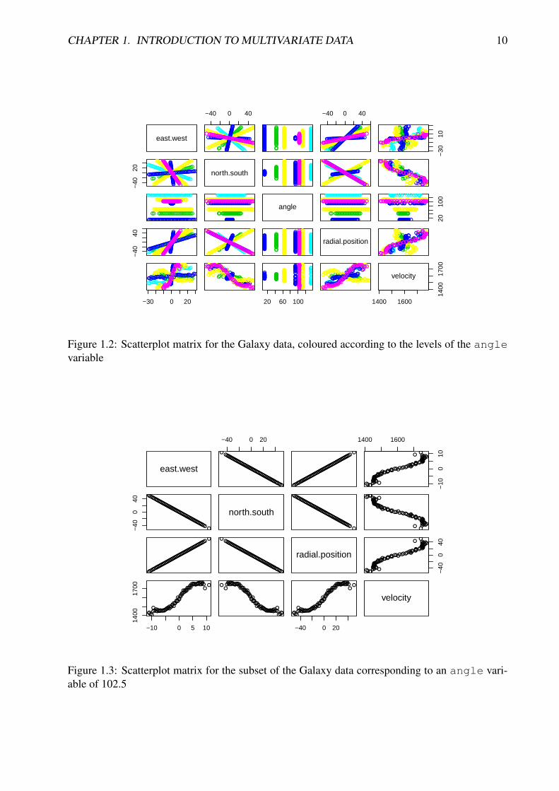
which shows that angle does indeed take on just 7 distinct values, and hence perhapshas more in common with an ordered categorical variable than a real-valued variable. Wecan use angle as a factor to colour the scatterplot as follows
pairs(galaxy,col=galaxy$angle)
to obtain the plot shown in Figure 1.2.This new plot indicates that there appear to be rather simple relationships between the
variables, but that those relationships change according to the level of the angle “factor”.We can focus in on one particular value of angle in the following way
pairs(galaxy[galaxy$angle==102.5,-3])
Note the use of -3 to drop the third (angle) column from the data frame. The new plot isshown in Figure 1.3.
This plot reveals that (for a given fixed value of angle) there is a simple deterministiclinear relationship between the first three variables (and so these could be reduced tojust one variable), and that there is a largely monotonic “S”-shaped relationship betweenvelocity and (say) radial.position. So with just a few simple scatterplot matrices andsome simple R commands we have reduced this multivariate data frame with apparently5 quantitative variables to just 2 quantitative variables plus an ordered categorical factor.It is not quite as simple as this, as the relationships between the three positional variablesvaries with the level of angle, but we have nevertheless found a lot of simple structurewithin the data set with some very basic investigation.
CHAPTER 1. INTRODUCTION TO MULTIVARIATE DATA 10
east.west
−40 0 40
●●●●●●●●●●●●●●●●●●●●●●●●●●●●●●●●●●●●●
●●●●●●●●●●●●●●●●●●●●●●●●
●●●●●●●●●●●●●●●●●●●●●●●●●●●●●●●●●●●
●●●●●●●●●●●●●●●●●●●●●●●●●●●●●●●●●●●●●●●●●●●●●
●●●●●●●●●●●●●●●●●●●●●●●●●●●●
●●●●●●●●●●●●●●●●●●●●●●●●●●●●●●●●●●●●●●
●●●●●●●●●●●●●●●●●●●●●●●●●●●●●●●●●●●●●●●●●●●●●●
●●●●●●●●●●●●●●●●●●●●●●●●●●●
●●●●●●●●●●●●●●●●●●●●●●●●●●●●●●●●●●●●●●●●●●●
●●●●●●●●●●●●●●●●●●●●●●●●●●●●●●●●●●●●●
●●●●●●●●●●●●●●●●●●●●●●●●
●●●●●●●●●●●●●●●●●●●●●●●●●●●●●●●●●●●
●●●●●●●●●●●●●●●●●●●●●●●●●●●●●●●●●●●●●●●●●●●●●
●●●●●●●●●●●●●●●●●●●●●●●●●●●●
●●●●●●●●●●●●●●●●●●●●●●●●●●●●●●●●●●●●●●
●●●●●●●●●●●●●●●●●●●●●●●●●●●●●●●●●●●●●●●●●●●●●●
●●●●●●●●●●●●●●●●●●●●●●●●●●●
●●●●●●●●●●●●●●●●●●●●●●●●●●●●●●●●●●●●●●●●●●●
−40 0 40
●●●●●●●●●●●●●●●●●●●●●●●●●●●●●●●●●●●●●
●●●●●●●●●●●●●●●●●●●●●●●●
●●●●●●●●●●●●●●●●●●●●●●●●●●●●●●●●●●●
●●●●●●●●●●●●●●●●●●●●●●●●●●●●●●●●●●●●●●●●●●●●●
●●●●●●●●●●●●●●●●●●●●●●●●●●●●
●●●●●●●●●●●●●●●●●●●●●●●●●●●●●●●●●●●●●●
●●●●●●●●●●●●●●●●●●●●●●●●●●●●●●●●●●●●●●●●●●●●●●
●●●●●●●●●●●●●●●●●●●●●●●●●●●
●●●●●●●●●●●●●●●●●●●●●●●●●●●●●●●●●●●●●●●●●●●
−30
10●●●●●●●●●●●●●●●●●●●●●●●●●●●●●●●●●●● ●●
●●●●●●●●● ●●●●●●●●●●●●●●●
●●●●●●●●●●●●●●●●●●●●●●●●●●●●●●●●●●●
●●●●●● ●●●●●●●●●●●●●●●●●●●●●●●●●●●●●●●●●●●●●●●
●●●●●●●●●●●●●●●●●●●● ●●●●● ●●●
●● ●●● ●●●●●●●●● ●●●●●●●●●●●●●●●●●●●●●●●●
●●●●●●●●●●●●●●●●●●●●●●●●● ●●●●●●●●●●●●●●●● ●●●●●
●●●●●●●●●●●●●●●●●●●●●●●●●●●
●● ●●●●●●●●●●●●●●●●●●●●●●●●●●●●●●●●●●●●●●●●●
−40
20
●●●●●●●●
●●●●●●●●
●●●●●●●●
●●●●●●●●
●●●●●
●●●●●●●●●●●●●●●●●●●●●●●●●●●●●
●●●●●●●●●●
●●●●●●●●●●
●●●●●●●●●●
●●●●●●●●
●●●●●●●●
●●●●●●●●
●●●●●●●●
●●●●●●●●
●●●●●
●●●●●●●●●●●●●●●●●●●●●●●●●●●●
●●●●●●●●●●●●●●●●●●●●●●●●●●●●●●●●●●●●●●
●●●●●●●●●●●●●●●●●●●●●●●●●●●●●●●●●●●●●●●●●●●●●●
●●●●●●●●●●●●●●●●●●●●●●●●●●●
●●●●●●
●●●●●●●●
●●●●●●●●
●●●●●●●●
●●●●●●●●
●●●●●
north.south●●●●●●●●●●●●●●●●●●●●●●●●●●●●●●●●●●●●●
●●●●●●●●●●●●●●●●●●●●●●●●●●●●●●●●●●●●●●●●●●●●●●●●●●●●●●●●●●●
●●●●●●●●●●●●●●●●●●●●●●●●●●●●●●●●●●●●●●●●●●●●●
●●●●●●●●●●●●●●●●●●●●●●●●●●●●
●●●●●●●●●●●●●●●●●●●●●●●●●●●●●●●●●●●●●●
●●●●●●●●●●●●●●●●●●●●●●●●●●●●●●●●●●●●●●●●●●●●●●
●●●●●●●●●●●●●●●●●●●●●●●●●●●
●●●●●●●●●●●●●●●●●●●●●●●●●●●●●●●●●●●●●●●●●●●
●●●●●●●●
●●●●●●●●
●●●●●●●●
●●●●●●●●
●●●●●
●●●●●●●●●●●●●●●●●●●●●●●●●●●●●
●●●●●●●●●●
●●●●●●●●●●
●●●●●●●●●●
●●●●●●●●
●●●●●●●●
●●●●●●●●
●●●●●●●●
●●●●●●●●
●●●●●
●●●●●●●●●●●●●●●●●●●●●●●●●●●●
●●●●●●●●●
●●●●●●●●
●●●●●●●●
●●●●●●●●
●●●●● ●●●●●●●●●●●●●●●●●●●●●●●●●●●●●●●●●●●●●●●●●●●●●●
●●●●●●●●●●●●●●●●●●●●●●●●●●●
●●●●●●●●●
●●●●●●●●
●●●●●●●●
●●●●●●●●
●●●●●●●●
●●
●●●●●●●●●●●●●●●●●●●●●●●●●●●
●●●●●●●● ●●
●●●●●●●●● ●●●●●●●●●●●●●●●●●●●●●●●●●●●●●●●●●●●●●●●●●
●●●●●●●●●
●●●●●● ●●●●
●●●●●●●●●●●●●●●●●●●●●●●
●●●●●●●●●●●●
●●●●●●●●●●●●●●●●●●●● ●●●●● ●●●
●● ●●● ●●●●●●●●● ●●●●●●●●●●●
●●●●●●●●●
●●●●●●●●●●●●●●●●●●●●●●●●●●●●● ●●●●●●●●●●●●●●●● ●●●●●
●●●●●●●●●●●●●●●●●●●●●●●●●●●
●● ●●●●●●●●●●
●●●●●●●●●●●●●●●●●●●●●●●●●●●●●●●
●●●●●●●●●●●●●●●●●●●●●●●●●●●●●●●●●●●●●
●●●●●●●●●●●●●●●●●●●●●●●●
●●●●●●●●●●●●●●●●●●●●●●●●●●●●●●●●●●●●●●●●●●●●●●●●●●●●●●●●●●●●●●●●●●●●●●●●●●●●●●●●
●●●●●●●●●●●●●●●●●●●●●●●●●●●●
●●●●●●●●●●●●●●●●●●●●●●●●●●●●●●●●●●●●●●
●●●●●●●●●●●●●●●●●●●●●●●●●●●●●●●●●●●●●●●●●●●●●●
●●●●●●●●●●●●●●●●●●●●●●●●●●●
●●●●●●●●●●●●●●●●●●●●●●●●●●●●●●●●●●●●●●●●●●● ●●●●●●●●●●●●●●●●●●●●●●●●●●●●●●●●●●●●●
●●●●●●●●●●●●●●●●●●●●●●●●
●●●●●●●●●●●●●●●●●●●●●●●●●●●●●●●●●●●●●●●●●●●●●●●●●●●●●●●●●●●●●●●●●●●●●●●●●●●●●●●●
●●●●●●●●●●●●●●●●●●●●●●●●●●●●
●●●●●●●●●●●●●●●●●●●●●●●●●●●●●●●●●●●●●●
●●●●●●●●●●●●●●●●●●●●●●●●●●●●●●●●●●●●●●●●●●●●●●
●●●●●●●●●●●●●●●●●●●●●●●●●●●
●●●●●●●●●●●●●●●●●●●●●●●●●●●●●●●●●●●●●●●●●●●
angle●●●●●●●●●●●●●●●●●●●●●●●●●●●●●●●●●●●●●
●●●●●●●●●●●●●●●●●●●●●●●●
●●●●●●●●●●●●●●●●●●●●●●●●●●●●●●●●●●●●●●●●●●●●●●●●●●●●●●●●●●●●●●●●●●●●●●●●●●●●●●●●
●●●●●●●●●●●●●●●●●●●●●●●●●●●●
●●●●●●●●●●●●●●●●●●●●●●●●●●●●●●●●●●●●●●
●●●●●●●●●●●●●●●●●●●●●●●●●●●●●●●●●●●●●●●●●●●●●●
●●●●●●●●●●●●●●●●●●●●●●●●●●●
●●●●●●●●●●●●●●●●●●●●●●●●●●●●●●●●●●●●●●●●●●●
2010
0
●●●●●●●●●●●●●●●●●●●●●●●●●●●●●●●●●●● ●●
●●●●●●●●● ●●●●●●●●●●●●●●●
●●●●●●●●●●●●●●●●●●●●●●●●●●●●●●●●●●●●●●●●● ●●●●●●●●●●●●●●●●●●●●●●●●●●●●●●●●●●●●●●●
●●●●●●●●●●●●●●●●●●●● ●●●●● ●●●
●● ●●● ●●●●●●●●● ●●●●●●●●●●●●●●●●●●●●●●●●
●●●●●●●●●●●●●●●●●●●●●●●●● ●●●●●●●●●●●●●●●● ●●●●●
●●●●●●●●●●●●●●●●●●●●●●●●●●●
●● ●●●●●●●●●●●●●●●●●●●●●●●●●●●●●●●●●●●●●●●●●
−40
40 ●●●●●●●●●●●●●●●●●●●●●●●●●●●●●●●●●●●●●
●●●●●●●●●●●●●●●●●●●●●●●●
●●●●●●●●●●●●●●●●●●●●●●●●●●●●●●●●●●●
●●●●●●●●●●●●●●●●●●●●●●●●●●●●●●●●●●●●●●●●●●●●●
●●●●●●●●●●●●●●●●●●●●●●●●●●●●
●●●●●●●●●●●●●●●●●●●●●●●●●●●●●●●●●●●●●●
●●●●●●●●●●●●●●●●●●●●●●●●●●●●●●●●●●●●●●●●●●●●●●
●●●●●●●●●●●●●●●●●●●●●●●●●●●
●●●●●●●●●●●●●●●●●●●●●●●●●●●●●●●●●●●●●●●●●●●
●●●●●●●●●●●●●●●●●●●●●●●●●●●●●●●●●●●●●
●●●●●●●●●●●●●●●●●●●●●●●●
●●●●●●●●●●●●●●●●●●●●●●●●●●●●●●●●●●●
●●●●●●●●●●●●●●●●●●●●●●●●●●●●●●●●●●●●●●●●●●●●●
●●●●●●●●●●●●●●●●●●●●●●●●●●●●
●●●●●●●●●●●●●●●●●●●●●●●●●●●●●●●●●●●●●●
●●●●●●●●●●●●●●●●●●●●●●●●●●●●●●●●●●●●●●●●●●●●●●
●●●●●●●●●●●●●●●●●●●●●●●●●●●
●●●●●●●●●●●●●●●●●●●●●●●●●●●●●●●●●●●●●●●●●●●
●●●●●●●●●●●●●●●●●●●●●●●●●●●●●●●●●●●●●
●●●●●●●●●●●●●●●●●●●●●●●●
●●●●●●●●●●●●●●●●●●●●●●●●●●●●●●●●●●●
●●●●●●●●●●●●●●●●●●●●●●●●●●●●●●●●●●●●●●●●●●●●●
●●●●●●●●●●●●●●●●●●●●●●●●●●●●
●●●●●●●●●●●●●●●●●●●●●●●●●●●●●●●●●●●●●●
●●●●●●●●●●●●●●●●●●●●●●●●●●●●●●●●●●●●●●●●●●●●●●
●●●●●●●●●●●●●●●●●●●●●●●●●●●
●●●●●●●●●●●●●●●●●●●●●●●●●●●●●●●●●●●●●●●●●●●
radial.position●●●●●●●●●●●●●●●●●●●●●●●●●●●●●●●●●●● ●●
●●●●●●●●● ●●●●●●●●●●●●●●●
●●●●●●●●●●●●●●●●●●●●●●●●●●●●●●●●●●●
●●●●●● ●●●●●●●●●●●●●●●●●●●●●●●●●●●●●●●●●●●●●●●
●●●●●●●●●●●●●●●●●●●● ●●●●● ●●●
●● ●●● ●●●●●●●●● ●●●●●●●●●●●●●●●●●●●●●●●●
●●●●●●●●●●●●●●●●●●●●●●●●● ●●●●●●●●●●●●●●●● ●●●●●
●●●●●●●●●●●●●●●●●●●●●●●●●●●
●● ●●●●●●●●●●●●●●●●●●●●●●●●●●●●●●●●●●●●●●●●●
−30 0 20
●●●●●●●●●●●●●●●●●
●●●●●●●●●●●●●●●●●●
●●
●●●●●●●●●●
●●●●●●●●●●●●●●
●●●●●●●●●●●●●●●●●●●●●●●●●●●●●●●●●●●
●●●●●
●●●●●●●●●●●
●●●
●●●●●●●●●●●●●●●●●●●●●●●●●●
●●●●●●●●●●●●●●
●●●●●
●●●
●●●
●●●
●●●●●●●●●●●●●●●●●●●●●●●●●●●●●●●●●●●●●●
●●●●●●●●●●●●●●●●●●●●●●●
●●●●●●
●●●●●
●●●●●●●●●●●● ●●●●●●●●●●●●
●●●●●●●●●●●●●●●
●●●●●●●●●●●●●●●●●●●●●●●●●●●●●●●●●●●●●●●●
●●●
●●●●●●●●●●●●●●●●●
●●●●●●●●●●●●●●●●●●
●●
●●●●●●●●●●●●●●●●
●●●●●●●●
●●●●●●●●●●●●●●●●●●●●●●●●●●●●●●●●●●●
●●●●●
●●●●●●●●●●●
●●●
●●●●●●●●●●●●●●●●●●●●●●●●●●
●●●●●●●●●●●●●●
●●●●●●●●
●●●●●●
●●●●●
●●●●●●●●●
●●●●●●●
●●●●●●●●●●●●●●●●●●●●●●●●●●●●●●●●●●●
●●●●●●●
●●●●●●●●●
●●●●●●●●●●●● ●●●●●●●●●●●●●●●●●●●●●●●●●●●
●●●●●●●●●●●●●●●●●●●●●●●●●●●●●●●●●●●●●●●●
●●●
20 60 100
●●●●●●●●●●●●●●●●●●●●●●●●●●●●●●●●●●●●●
●●●●●●●●●●●●●●●●●●●●●●●●
●●●●●●●●●●●●●●●●●●●●●●●●●●●●●●●●●●●
●●●●●●●●●●●●●●●●●●●
●●●●●●●●●●●●●●●●●●●●●●●●●●
●●●●●●●●●●●●●●●●●●●●●●●●●●●●
●●●●●●●●●●●●●●●●●●●●●●●●●●●●●●●●●●●●●●
●●●●●●●●●●●●●●●●●●●●●●●●●●●●●●●●●●●●●●●●●●●●●●●●●●●●●●●●●●●●●●●●●●●●●●●●●
●●●●●●●●●●●●●●●●●●●●●●●●●●●●●●●●●●●●●●●●●●●
●●●●●●●●●●●●●●●●●
●●●●●●●●●●●●●●●●●●
●●
●●●●●●●●●●●●●●●●
●●●●●●●●
●●●●●●●●●●●●●●●●●●●●●●●●●●●●●●●●●●●
●●●●●
●●●●●●●●●●●
●●●
●●●●●●●●●●●●●●●●●●●●●●●●●●
●●●●●●●●●●●●●●
●●●●●●●●
●●●●●●
●●●●●
●●●●●●●●●
●●●●●●●
●●●●●●●●●●●●●●●●●●●●●●●●●●●●●●●●●●●
●●●●●●●
●●●●●●●●●
●●●●●●●●●●●● ●●●●●●●●●●●●●●●●●●●●●●●●●●●
●●●●●●●●●●●●●●●●●●●●●●●●●●●●●●●●●●●●●●●●
●●●
1400 1600
1400
1700
velocity
Figure 1.2: Scatterplot matrix for the Galaxy data, coloured according to the levels of the anglevariable
east.west
−40 0 20
●●●●●●●●●●●●●●●●●●●●●●●●●●●●●●●●●●●●●
●●●●●●●●●●●●●●●●●●●●●●●●●●●●●●●●●●●●●●●●●●●
●●●●●●●●●●●●●●●●●●●●●●●●●●●●●●●●●●●●●
●●●●●●●●●●●●●●●●●●●●●●●●●●●●●●●●●●●●●●●●●●●
1400 1600−
100
10●●●●●●●●●●●●●●●●●●●●●●●●●●●●●●●●●●● ●●
●● ●●●●●●●●●●●●●●●●●●●●●●●●●●●●●●●●●●●●●●●●●
−40
040
●●●●●●
●●●●●●
●●●●●●
●●●●●●
●●●●●●
●●●●●
●●
●●●●
●●●●●●
●●●●●●
●●●●●●
●●●●●●
●●●●●●
●●●●●●
●●●
north.south●●●
●●●●●●
●●●●●●
●●●●●●
●●●●●●
●●●●●●
●●●
●
●●●●
●●●●●●
●●●●●●
●●●●●●
●●●●●●
●●●●●●
●●●●●●
●●●
●●●●●●●●●●●●
●●●●●●●●●●●●●●●●●●●
●●●● ●●
●● ●●●●●
●●●●●●●●●●
●●●●●●●●●●●●●●●●
●●●●●●●●●●
●●●●●●●●●●●●●●●●●●●●●●●●●●●●●●●●●●●●●
●●●●●●●●●●●●●●●●●●●●●●●●●●●●●●●●●●●●●●●●●●●
●●●●●●●●●●●●●●●●●●●●●●●●●●●●●●●●●●●●●
●●●●●●●●●●●●●●●●●●●●●●●●●●●●●●●●●●●●●●●●●●●
radial.position
−40
040●●●●●●●●●●●●●●●●●●●●●●●●●●●●●●●●●●● ●
●
●● ●●●●●●●●●●●●●●●●●●●●●●●●●●●●●●●●●●●●●●●●●
−10 0 5 10
1400
1700
●●●●●●●●●●●●
●●●●●
●●●●
●●●●●●●●●●●●●●●
●
●●
●●●●●●●●●●●●●●●
●●●●
●●●●●●●●●●●●●●●●●●●
●●●
●●●●●●●●●●●●
●●●●●●●
●●●●●●●●●●●●●●●●
●●
●●●●
●●●●●●●●●●●●●●●
●●●●●●
●●●●●●●●●●●●●●●●●●
−40 0 20
●●●●●●●●●●●●
●●●●●
●●●●
●●●●●●●●●●●●●●●
●
●●
●●●●●●●●●●●●●●●
●●●●
●●●●●●●●●●●●●●●●●●●
●●●
velocity
Figure 1.3: Scatterplot matrix for the subset of the Galaxy data corresponding to an angle vari-able of 102.5
CHAPTER 1. INTRODUCTION TO MULTIVARIATE DATA 11
Example: Microarray data
The dataset nci represents measurements of the expression levels of 6,830 genes in64 different tissue samples taken from cancerous tumors. The first thing we need tothink about here is what the rows and columns should be. Which is n and which is p?The R command class(nci) reveals that this data set is actually stored as a matrixand not a data frame, so that is no help. The command dim(nci) indicates that thematrix is stored with 6,830 rows and 64 columns, but matrices can be easily transposedusing the t() command, so that doesn’t really tell us anything other than how the datahappens to be stored. This problem can arise whenever a multivariate data set consists ofmeasurements of exactly the same type in all rows and columns. Here the measurementsare expression levels (basically, a measure of the amount of a particular kind of mRNA in asample). Since all measurements have essentially the same units, and can be stored in amatrix, it is technically arbitrary which should be considered rows and columns. However,from the viewpoint of multivariate data analysis, it matters a great deal.
Here, fundamentally, the observations are 64 different tissue samples, and the vari-ables are the 6,830 genes, so n = 64 and p = 6, 830, so in some sense the nci matrixshould be transposed. However, it is common practice to store microarray data this way,and sometimes for certain analyses people really do take the genes to be the observa-tions and the samples to be the variables. Generally with multivariate analysis we wishto use observations to learn about the relationship between the variables. This data setis no exception, in that we wish to use the samples in order to learn something aboutthe relationship between the genes. Sometimes people work with the transposed datain order to use the genes in order to learn something about the relationship between thesamples. However, at a fundamental level, the measurements are of the amount of aparticular gene, in units specific to that gene, and in (essentially) identical units for eachsample. So it is really the genes that represent the variables, as columns of the sametype, in some sense...
There is actually something very special about this data in that p > n, and in fact,p >> n (p is much bigger than n). Multivariate data with this property is often referred toas “wide data” (as opposed to the more normal “tall data”), for obvious reasons. This isquite different to the other examples we have looked at, and rather atypical of classicalmultivariate data. Indeed, many of the classical statistical techniques we shall examine inthis course actually require n > p, and ideally need n >> p in order to work well. Datawith p > n will cause many classical algorithms to fail (and this is one reason why peoplesometimes work with the transposed data). We will revisit this issue at appropriate pointsin the course, and look at some simple techniques for analysing wide data near the endof the course.
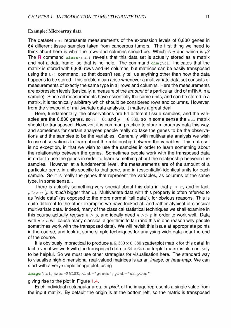
It is obviously impractical to produce a 6, 380× 6, 380 scatterplot matrix for this data! Infact, even if we work with the transposed data, a 64× 64 scatterplot matrix is also unlikelyto be helpful. So we must use other strategies for visualisation here. The standard wayto visualise high-dimensional real-valued matrices is as an image, or heat-map. We canstart with a very simple image plot, using
image(nci,axes=FALSE,xlab="genes",ylab="samples")
giving rise to the plot in Figure 1.4.Each individual rectangular area, or pixel, of the image represents a single value from
the input matrix. By default the origin is at the bottom left, so the matrix is transposed
CHAPTER 1. INTRODUCTION TO MULTIVARIATE DATA 12
Figure 1.4: Image plot of the nci cancer tumor microarray data, using the default colour scheme
(or rather, rotated anti-clockwise). Using the default “heat” colour scheme, low valuesare represented as “cold” red colours, and “hot” bright yellow/white colours represent thehigh values. Although many people find this colour scheme intuitive, it is not withoutproblems, and in particular, can be especially problematic for colour-blind individuals. Wecan produce a simple greyscale image usingimage(nci,axes=FALSE,xlab="genes",ylab="samples",col=grey((0:31)/31))
which has the lightest colours for the highest values, or usingimage(nci,axes=FALSE,xlab="genes",ylab="samples",col=grey((31:0)/31))
to make the highest values coloured dark. Another popular colouring scheme is providedby cm.colors(), which uses cyan for low values, magenta for high values, and middlevalues white. It is good for picking out extreme values, and can be used asimage(nci,axes=FALSE,xlab="genes",ylab="samples",col=cm.colors(32))
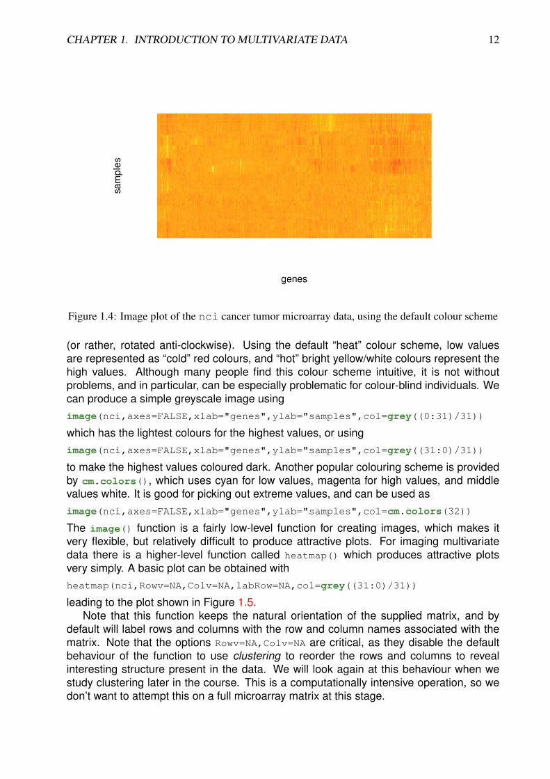
The image() function is a fairly low-level function for creating images, which makes itvery flexible, but relatively difficult to produce attractive plots. For imaging multivariatedata there is a higher-level function called heatmap() which produces attractive plotsvery simply. A basic plot can be obtained withheatmap(nci,Rowv=NA,Colv=NA,labRow=NA,col=grey((31:0)/31))
leading to the plot shown in Figure 1.5.Note that this function keeps the natural orientation of the supplied matrix, and by
default will label rows and columns with the row and column names associated with thematrix. Note that the options Rowv=NA,Colv=NA are critical, as they disable the defaultbehaviour of the function to use clustering to reorder the rows and columns to revealinteresting structure present in the data. We will look again at this behaviour when westudy clustering later in the course. This is a computationally intensive operation, so wedon’t want to attempt this on a full microarray matrix at this stage.
CHAPTER 1. INTRODUCTION TO MULTIVARIATE DATA 13
Figure 1.5: Heatmap of the nci cancer tumor microarray data, using a greyscale colour schemewith darker shades for higher values
Example: Handwritten digit images
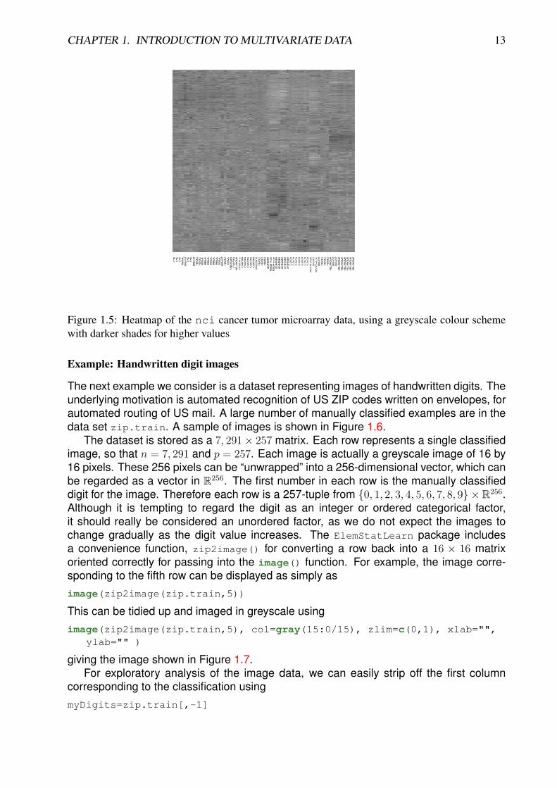
The next example we consider is a dataset representing images of handwritten digits. Theunderlying motivation is automated recognition of US ZIP codes written on envelopes, forautomated routing of US mail. A large number of manually classified examples are in thedata set zip.train. A sample of images is shown in Figure 1.6.
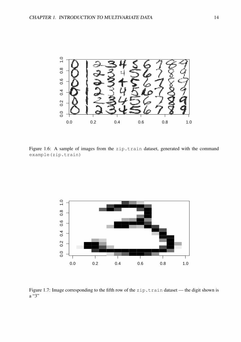
The dataset is stored as a 7, 291× 257 matrix. Each row represents a single classifiedimage, so that n = 7, 291 and p = 257. Each image is actually a greyscale image of 16 by16 pixels. These 256 pixels can be “unwrapped” into a 256-dimensional vector, which canbe regarded as a vector in R256. The first number in each row is the manually classifieddigit for the image. Therefore each row is a 257-tuple from {0, 1, 2, 3, 4, 5, 6, 7, 8, 9} × R256.Although it is tempting to regard the digit as an integer or ordered categorical factor,it should really be considered an unordered factor, as we do not expect the images tochange gradually as the digit value increases. The ElemStatLearn package includesa convenience function, zip2image() for converting a row back into a 16 × 16 matrixoriented correctly for passing into the image() function. For example, the image corre-sponding to the fifth row can be displayed as simply as
image(zip2image(zip.train,5))
This can be tidied up and imaged in greyscale using
image(zip2image(zip.train,5), col=gray(15:0/15), zlim=c(0,1), xlab="",ylab="" )
giving the image shown in Figure 1.7.For exploratory analysis of the image data, we can easily strip off the first column
corresponding to the classification using
myDigits=zip.train[,-1]
CHAPTER 1. INTRODUCTION TO MULTIVARIATE DATA 14
0.0 0.2 0.4 0.6 0.8 1.0
0.0
0.2
0.4
0.6
0.8
1.0
Figure 1.6: A sample of images from the zip.train dataset, generated with the commandexample(zip.train)
0.0 0.2 0.4 0.6 0.8 1.0
0.0
0.2
0.4
0.6
0.8
1.0
Figure 1.7: Image corresponding to the fifth row of the zip.train dataset — the digit shown isa “3”
CHAPTER 1. INTRODUCTION TO MULTIVARIATE DATA 15
to give a multivariate dataset with n = 7, 291 and p = 256, where each row representsa vector in R256. It is perhaps concerning that representing the images as a vector inR256 loses some important information about the structure of the data — namely that it isactually a 16 × 16 matrix. So, for example, we know that the 2nd and 18th elements ofthe 256-dimensional vector actually correspond to adjacent pixels, and hence are likely tobe highly correlated. This is clearly valuable information that we aren’t explicitly includinginto our framework. The idea behind “data mining” is that given a sufficiently large numberof example images, it should be possible to “learn” that the 2nd and 18th elements arehighly correlated without explicitly building this in to our modelling framework in the firstplace. We will look at how we can use data on observations to learn about the relationshipbetween variables once we have the appropriate mathematical framework set up.
1.3 Representing and summarising multivariate data
Clearly an important special case of (multivariate) data frames arises when the p variablesare all real-valued and so the data can be regarded as an n×p real-valued matrix. We sawin the previous example that even when the original data is not in exactly this format, it isoften possible to extract a subset of variables (or otherwise transform the original data) togive a new dataset which does have this form. This is the classical form of a multivariatedataset, and many classical modelling and analysis techniques of multivariate statisticsare tailored specifically to data of this simple form. Classically, as we have seen, therows of the matrix correspond to observations, and the columns correspond to variables.However, it is often convenient to regard the observations as column vectors, and so caremust be taken when working with multivariate data mathematically to transpose rows froma data matrix in order to get a column vector representing an observation.
Definition 1 The measurement of the jth variable on the ith observation is denoted xij,and is stored in the ith row and jth column of an n× p matrix denoted by X, known as thedata matrix.
However, we use xi to denote a column vector corresponding to the ith observation,and hence the ith row of X. That is
xi = (xi1, xi2, . . . , xip)T =
xi1xi2...xip
.
We denote the column vector representing the jth variable by x(j), which we can obviouslydefine directly as
x(j) =
x1jx2j...xnj
.
We can begin to think about summarising multivariate data by applying univariate sum-maries that we already know about to the individual variables.

CHAPTER 1. INTRODUCTION TO MULTIVARIATE DATA 16
1.3.1 The sample mean
As a concrete example, it is natural to be interested in the sample mean of each variable.The sample mean of x(j) is denoted xj, and is clearly given by
xj =1
n
n∑i=1
xij.
We can compute xj for j = 1, 2, . . . , p, and then collect these sample means together intoa p-vector that we denote x, given by
x = (x1, x2, . . . , xp)T.
Note, however, that we could have defined x more directly as follows.
Definition 2 The sample mean of the n × p data matrix, X, is the p-vector given by thesample mean of the observation vectors,
x =1
n
n∑i=1
xi.
A moments thought reveals that this is equivalent to our previous construction. The vec-tor version is more useful however, as we can use it to build an even more convenientexpression directly in terms of the data matrix, X. For this we need notation for a vectorof ones. For an n-vector of ones, we use the notation 11n, so that
11n ≡ (1, 1, . . . , 1)T.
We will sometimes drop the subscript if the dimension is clear from the context. Note that11n
T11n = n (an inner product), and that 11n11pT is an n×p matrix of ones (an outer product),
sometimes denoted Jn×p. Pre- or post-multiplying a matrix by a row or column vector ofones has the effect of summing over rows or columns. In particular, we can now write thesample mean of observation vectors as follows.
Proposition 1 The sample mean of a data matrix can be computed as
x =1
nXT11n.
Example: Galaxy data
The R command summary() applies some univariate summary statistics to each vari-able in a data frame separately, and this can provide some useful information about theindividual variables that make up the data frame> summary ( galaxy )
east . west nor th . south angle r a d i a l . p o s i t i o nMin . :−29.66693 Min . :−49.108 Min . : 12.50 Min . :−52.40001 s t Qu . : −7.91687 1 s t Qu.:−13.554 1 s t Qu . : 63.50 1 s t Qu.:−21.3500Median : −0.06493 Median : 0.671 Median : 92.50 Median : −0.8000Mean : −0.33237 Mean : 1.521 Mean : 80.89 Mean : −0.84273rd Qu . : 6.95053 3rd Qu . : 18.014 3rd Qu. :102 .50 3rd Qu . : 19.6500Max . : 29.48414 Max . : 49.889 Max . :133.00 Max . : 55.7000
v e l o c i t y

CHAPTER 1. INTRODUCTION TO MULTIVARIATE DATA 17
Min . :14091 s t Qu. :1523Median :1586Mean :15943rd Qu. :1669Max . :1775
>
The apply() command can also be used to apply arbitrary functions to the rows orcolumns of a matrix. Here we can obtain the mean vector using> apply ( galaxy ,2 ,mean)
east . west nor th . south angle r a d i a l . p o s i t i o n v e l o c i t y−0.3323685 1.5210889 80.8900929 −0.8427245 1593.6253870
>
The 2 is used to indicate that we wish to apply the function to each column in turn. Ifwe had instead used 1, the mean of each row of the matrix would have been computed(which would have been much less interesting). We can also use our matrix expressionto directly compute the mean from the data matrix> as . vector ( t ( galaxy ) %∗% rep (1 ,323) /323)[ 1 ] −0.3323685 1.5210889 80.8900929 −0.8427245 1593.6253870>
where %*% is the matrix multiplication operator in R. Since R helpfully transposes vectorsas required according to the context, we can actually compute this more neatly using
> rep(1,nrow(galaxy))%*%as.matrix(galaxy)/nrow(galaxy)east.west north.south angle radial.position velocity
[1,] -0.3323685 1.521089 80.89009 -0.8427245 1593.625>
It is typically much faster to use matrix operations than the apply() command. Notehowever, that R includes a convenience function, colMeans() for computing the samplemean of a data frame:
> colMeans(galaxy)east.west north.south angle radial.position-0.3323685 1.5210889 80.8900929 -0.8427245
velocity1593.6253870
and so it will usually be most convenient to use that.
Example: toy problem
Before moving on, it is worth working through a very small, simple toy problem by hand,in order to make sure that the ideas are all clear. Suppose that we have measured theheight (in metres) and weight (in kilograms) of 5 students. We have n = 5 and p = 2, andthe data matrix is as follows
X =
1.67 65.01.78 85.01.60 54.51.83 72.01.80 94.5
We can calculate the mean vector, x for this data matrix in three different ways. First startby calculating the column means.

CHAPTER 1. INTRODUCTION TO MULTIVARIATE DATA 18
For x1 we have
x1 =1
n
n∑i=1
xi1 =1
5(1.67 + 1.78 + 1.60 + 1.83 + 1.80)
=8.68
5= 1.736,
and similarly
x2 =1
5(65.0 + 85.0 + 54.5 + 72.0 + 94.5) = 74.2.
So our mean vector is
x = (1.736, 74.2)T.
Next we can calculate it as the sample mean of the observa-tion vectors as
x =1
n
n∑i=1
xi =1
5
[(1.67
65.0
)+
(1.78
85.0
)+
(1.60
54.5
)+
(1.83
72.0
)+
(1.80
94.5
)]=
(1.736
74.2
).
Finally, we can use our matrix expression for the sample mean
x =1
nXT11n =
1
5
(1.67 1.78 1.60 1.83 1.8065.0 85.0 54.5 72.0 94.5
)11111
=1
5
(8.68
371.00
)=
(1.736
74.2
).
This example hopefully makes clear that our three different ways of thinking about com-puting the sample mean are all equivalent. However, the final method based on a matrixmultiplication operation is the neatest both mathematically and computationally, and sowe will make use of this expression, as well as other similar expressions, throughout thecourse.
1.3.2 Sample variance and covariance
Just as for the mean, we can think about other summaries starting from univariate sum-maries applied to the individual variables of the data matrix. We write the sample variance
CHAPTER 1. INTRODUCTION TO MULTIVARIATE DATA 19
of x(j) as s2j or sjj, and calculate as
sjj =1
n− 1
n∑i=1
(xij − xj)2.
Similarly, we can calculate the sample covariance between variables j and k as
sjk =1
n− 1
n∑i=1
(xij − xj)(xik − xk),
which clearly reduces to the sample variance when k = j. If we compute the samplecovariances for all j, k = 1, 2, . . . , p, then we can use them to form a p× p matrix,
S =
s11 s12 · · · s1ps21 s22 · · · s2p...
... . . . ...sp1 sp2 · · · spp
,
known as the sample covariance matrix, or sample variance matrix, or sometimes as thesample variance-covariance matrix. Again, a with a little thought, one can see that wecan construct this matrix directly from the observation vectors.
Definition 3 The sample variance matrix is defined by
S =1
n− 1
n∑i=1
(xi − x)(xi − x)T.
This expression is much simpler than computing each component individually, but can besimplified further if we consider the problem of centering the data.
We can obviously write the sample covariance matrix as
S =1
n− 1
n∑i=1
wiwiT,
where wi = xi − x, i = 1, 2, . . . , n, and we can regard the wi as observations from a newn× p data matrix W. We can construct W as
W = X−
xT
xT
...xT
= X− 11nx
T
= X− 11n
[1
nXT11n
]T
= X− 1
n11n11n
TX
=
(In×n−
1
n11n11n
T
)X
= HnX,
where

CHAPTER 1. INTRODUCTION TO MULTIVARIATE DATA 20
Definition 4Hn ≡ In×n−
1
n11n11n
T
is known as the centering matrix.
So we can subtract the mean from a data matrix by pre-multiplying by the centering matrix.This isn’t a numerically efficient way to strip out the mean, but is mathematically elegantand convenient. The centering matrix has several useful properties that we can exploit.
Proposition 2 The centering matrix Hn has the following properties:
1. Hn is symmetric, HnT = Hn,
2. Hn is idempotent, H2n = Hn,
3. If X is an n× p data matrix, then the n× p matrix W = HnX has sample mean equalto the zero p-vector.
ProofThese are trivial exercises in matrix algebra. 1. and 2. are left as exercises. We will
use symmetry to show 3.
w =1
nWT11n
=1
n(HnX)T11n
=1
nXTHn11n
=1
nXT(In×n−
1
n11n11n
T)11n
=1
nXT(11n −
1
n11n11n
T11n)
=1
nXT(11n − 11n)
= 0.
�
Re-writing the sample variance matrix, S, in terms of the centered data matrix W, is useful,since we can now simplify the expression further. We first write
n∑i=1
wiwiT = (w1,w2, . . . ,wn)
w1
T
w2T
...wn
T
= WTW,

CHAPTER 1. INTRODUCTION TO MULTIVARIATE DATA 21
using properties of block matrix multiplication. From this we conclude that
S =1
n− 1
n∑i=1
wiwiT =
1
n− 1WTW
We can then substitute back in our definition of W using the centering matrix to get
S =1
n− 1WTW =
1
n− 1(HnX)THnX =
1
n− 1XTHn
THnX =1
n− 1XTHnX,
using symmetry and idempotency of Hn. This gives us the rather elegant result:
Proposition 3 The sample variance matrix can be written
S =1
n− 1XTHnX.
We shall make considerable use of this result.
Example: galaxy data
With the galaxy data, we can start by computing the column variances with
> apply(galaxy,2,var)east.west north.south angle radial.position144.6609 523.8497 1462.6269 670.2299velocity
8886.4772
which gives diagonal elements consistent with the built-in var() function:
> var(galaxy)east.west north.south angle radial.position
east.west 144.66088 -32.67993 -21.50402 263.93661north.south -32.67993 523.84971 26.35728 -261.78938angle -21.50402 26.35728 1462.62686 -49.01139radial.position 263.93661 -261.78938 -49.01139 670.22991velocity 451.46551 -1929.95131 37.21646 1637.78301
velocityeast.west 451.46551north.south -1929.95131angle 37.21646radial.position 1637.78301velocity 8886.47724
as can be verified with
> diag(var(galaxy))east.west north.south angle radial.position144.6609 523.8497 1462.6269 670.2299velocity
8886.4772
The built-in var() function is very efficient, and should generally be preferred as theway to compute a sample variance matrix in R. However, we can easily check that ourmathematically elegant matrix result works using

CHAPTER 1. INTRODUCTION TO MULTIVARIATE DATA 22
> H=diag(323)-matrix(1/323,ncol=323,nrow=323)> t(galaxy)%*%H%*%as.matrix(galaxy)/(323-1)
east.west north.south angle radial.positioneast.west 144.66088 -32.67993 -21.50402 263.93661north.south -32.67993 523.84971 26.35728 -261.78938angle -21.50402 26.35728 1462.62686 -49.01139radial.position 263.93661 -261.78938 -49.01139 670.22991velocity 451.46551 -1929.95131 37.21646 1637.78301
velocityeast.west 451.46551north.south -1929.95131angle 37.21646radial.position 1637.78301velocity 8886.47724
This method is clearly mathematically correct. However, the problem is that building then × n centering matrix and carrying out a matrix multiplication using it is a very compu-tationally inefficient way to simply strip the mean out of a data matrix. If we wanted toimplement our own method more efficiently, we could do it along the following lines
> Wt=t(galaxy)-colMeans(galaxy)> Wt %*% t(Wt)/(323-1)
east.west north.south angle radial.positioneast.west 144.66088 -32.67993 -21.50402 263.93661north.south -32.67993 523.84971 26.35728 -261.78938angle -21.50402 26.35728 1462.62686 -49.01139radial.position 263.93661 -261.78938 -49.01139 670.22991velocity 451.46551 -1929.95131 37.21646 1637.78301
velocityeast.west 451.46551north.south -1929.95131angle 37.21646radial.position 1637.78301velocity 8886.47724
This uses a couple of R tricks, relying on the fact that R stores matrices in column-majororder and “recycles” short vectors. We can improve on this slightly by directly constructingthe outer product 11nx
T.
> W=galaxy-outer(rep(1,323),colMeans(galaxy))> W=as.matrix(W)> t(W)%*%W/(323-1)
east.west north.south angle radial.positioneast.west 144.66088 -32.67993 -21.50402 263.93661north.south -32.67993 523.84971 26.35728 -261.78938angle -21.50402 26.35728 1462.62686 -49.01139radial.position 263.93661 -261.78938 -49.01139 670.22991velocity 451.46551 -1929.95131 37.21646 1637.78301
velocityeast.west 451.46551north.south -1929.95131angle 37.21646

CHAPTER 1. INTRODUCTION TO MULTIVARIATE DATA 23
radial.position 1637.78301velocity 8886.47724
In fact, we can do even better than this by exploiting the R function sweep(), which isintended to be used for exactly this sort of centering procedure, where some statistics areto be “swept” out of a data frame.
> W=as.matrix(sweep(galaxy,2,colMeans(galaxy)))> t(W)%*%W/(323-1)
east.west north.south angle radial.positioneast.west 144.66088 -32.67993 -21.50402 263.93661north.south -32.67993 523.84971 26.35728 -261.78938angle -21.50402 26.35728 1462.62686 -49.01139radial.position 263.93661 -261.78938 -49.01139 670.22991velocity 451.46551 -1929.95131 37.21646 1637.78301
velocityeast.west 451.46551north.south -1929.95131angle 37.21646radial.position 1637.78301velocity 8886.47724
Example: ZIP code digits
For our handwritten image data, we can easily compute the sample variance matrix forthe 256 columns corresponding to the image with
> v=var(zip.train[,-1])> dim(v)[1] 256 256> prod(dim(v))[1] 65536
There probably isn’t much point in printing the resulting 256 × 256 matrix to the screenand reading through all 65,536 covariances. However, we have already seen that we cansometimes use images to visualise large matrices, and we can also do that here
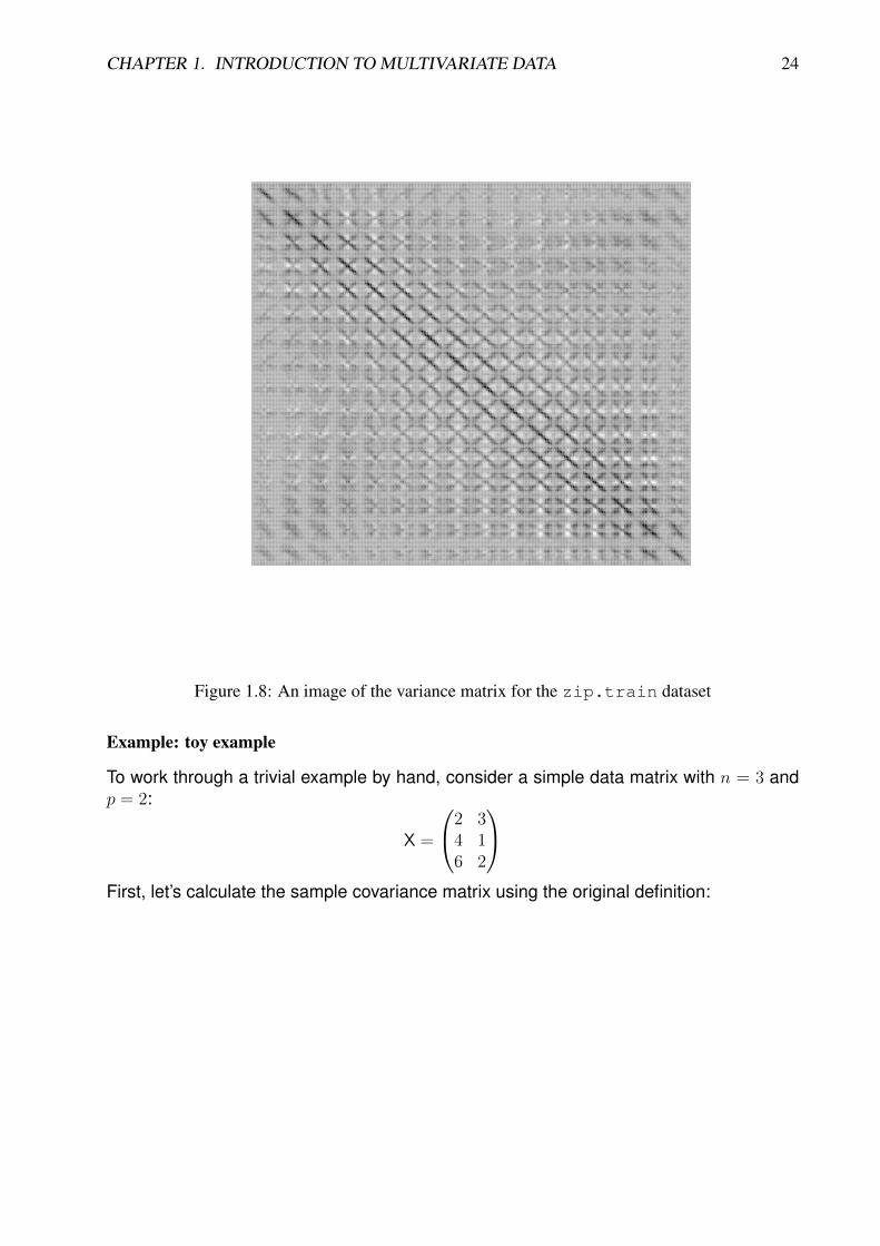
image(v[,256:1],col=gray(15:0/15),axes=FALSE)
giving the plot shown in Figure 1.8.The image shows a narrow dark band down the main diagonal corresponding to the
pixel variances, but alternating between dark and light, due to the pixels near the edgeof each row having relatively low variance (due to usually being blank). Then we seeparallel bands every 16 pixels due to pixels adjacent on consecutive rows being highlycorrelated. The bands perpendicular to the leading diagonal are at first a little moremysterious, but interestingly, these arise from the fact that many digits have a degree ofbilateral symmetry, with digits such as “1” and “8” being classic examples, but others suchas “6”, “5” and “2” also having some degree of bilateral symmetry.
CHAPTER 1. INTRODUCTION TO MULTIVARIATE DATA 24
Figure 1.8: An image of the variance matrix for the zip.train dataset
Example: toy example
To work through a trivial example by hand, consider a simple data matrix with n = 3 andp = 2:
X =
2 34 16 2
First, let’s calculate the sample covariance matrix using the original definition:
For this we first need to compute
x = (4, 2)T

CHAPTER 1. INTRODUCTION TO MULTIVARIATE DATA 25
Then we have
S =1
n− 1
n∑i=1
(xi − x)(xi − x)T
=1
2
{[(2
3
)−(
4
2
)][(2
3
)−(
4
2
)]T
+
[(4
1
)−(
4
2
)][(4
1
)−(
4
2
)]T
+
[(6
2
)−(
4
2
)][(6
2
)−(
4
2
)]T
}=
1
2
{(−2
1
)(−2, 1) +
(0
−1
)(0,−1) +
(2
0
)(2, 0)
}=
{(4 −2
−2 1
)+
(0 0
0 1
)+
(4 0
0 0
)}=
1
2
(8 −2
−2 2
)=
(4 −1
−1 1
)Next, let’s calculate using our formula based around the centering matrix
First calculate
H3 = I3−1
3113113
T =
23−13−13
−13
23−13
−13−13
23
,

CHAPTER 1. INTRODUCTION TO MULTIVARIATE DATA 26
and then use this to compute
S =1
n− 1XTHnX
=1
2
(2 4 6
3 1 2
) 23−13−13
−13
23−13
−13−13
23
2 3
4 1
6 2
=
1
2
(2 4 6
3 1 2
)−2 1
0 −1
2 0
=
1
2
(8 −2
−2 2
)=
(4 −1
−1 1
)Finally, let’s think about how to do this computation a little more efficiently. Let’s start
by constructing
W = X− 113xT =
−2 10 −12 0
Now
S =1
2WTW =
1
2
(−2 0 21 −1 0
)−2 10 −12 0
=
1
2
(8 −2−2 2
)=
(4 −1−1 1
)So, the variances of the variables are 4 and 1, and the covariance between them is -1,which indicates that the variables are negatively correlated.
Before moving on, it is worth dwelling a little more on the intermediate result
S =1
n− 1WTW,
which shows us that the matrix S factorises in a very nice way. We will return to matrixfactorisation later, but for now it is worth noting that we can re-write the above as
S = ATA
whereA =
1√n− 1
W.
Matrices which factorise in this way have two very important properties
CHAPTER 1. INTRODUCTION TO MULTIVARIATE DATA 27
Proposition 4 Let S be a p× p matrix of the form
S = ATA,
where A is an n× p matrix. Then S has the following properties:
1. S is symmetric, ST = S,
2. S is positive semi-definite (or non-negative definite), written S ≥ 0. This means thatαTSα ≥ 0 for all choices of p-vector α.
Proof
1. is trivial. For 2., note that
αTSα = αTATAα
= (Aα)T(Aα)
= ‖Aα‖22
≥ 0.
�
So the sample variance matrix is symmetric and non-negative definite.
1.3.3 Sample correlation
The sample correlation between variables i and j is defined by
rij =sijsisj
.
Clearly, from the definition of sample covariance we have that rii = 1, i = 1, 2, . . . , p, andputting w(i) = x(i) − xi11n,
rij =w(i)Tw(j)
√w(i)Tw(i)
√w(j)Tw(j)
=w(i) ·w(j)
‖w(i)‖‖w(j)‖
and so by the Cauchy-Schwarz inequality we have |rij| ≤ 1, i, j = 1, 2, . . . , p. As with thesample covariance matrix, we can create a p× p matrix of sample correlations, known asthe sample correlation matrix, R. If R = Ip, so that all off-diagonal correlations are zero,then we say that the variables are uncorrelated.
If we now define D to be the diagonal matrix of sample standard deviations, that is
D = diag{s1, s2, . . . , sp} =
s1 0 · · · 00 s2 · · · 0...
... . . . ...0 0 · · · sp
,
then we get the following result.

CHAPTER 1. INTRODUCTION TO MULTIVARIATE DATA 28
Proposition 5 The sample correlation matrix may be computed from the sample variancematrix as
R = D−1SD−1,
and conversely, the sample covariance matrix may be computed from the sample corre-lation matrix as
S = DRD.
ProofThis follows since pre-multiplying by a diagonal matrix re-scales the rows and post-
multiplying by a diagonal matrix re-scales the columns. �
Proposition 6 The sample correlation matrix is symmetric and positive semi-definite.
ProofWe have already shown that the sample covariance matrix can be written as S = ATA.
Consequently, R can be written asR = BTB,
where B = AD−1. We showed earlier that matrices that can be written in this form mustbe symmetric and positive semi-definite. �
Example: Galaxy data
Returning to the galaxy data example, we can compute the sample correlation matrixdirectly using the built-in R command cor() as follows
> cor(galaxy)east.west north.south angle radial.position
east.west 1.00000000 -0.11871407 -0.04674954 0.8476414north.south -0.11871407 1.00000000 0.03011136 -0.4418112angle -0.04674954 0.03011136 1.00000000 -0.0495015radial.position 0.84764144 -0.44181124 -0.04950150 1.0000000velocity 0.39818438 -0.89449554 0.01032294 0.6710883
velocityeast.west 0.39818438north.south -0.89449554angle 0.01032294radial.position 0.67108826velocity 1.00000000
So, for example, the correlation between radial position and velocity is 0.671, as we canverify with
> cor(galaxy$radial.position,galaxy$velocity)[1] 0.6710883
Using the built-in cor() function is the preferred way to compute a sample correlation ma-trix, as it is computationally efficient. Nevertheless, we can calculate using Proposition 5as

CHAPTER 1. INTRODUCTION TO MULTIVARIATE DATA 29
> diag(1/sd(galaxy)) %*% var(galaxy) %*% diag(1/sd(galaxy))[,1] [,2] [,3] [,4] [,5]
[1,] 1.00000000 -0.11871407 -0.04674954 0.8476414 0.39818438[2,] -0.11871407 1.00000000 0.03011136 -0.4418112 -0.89449554[3,] -0.04674954 0.03011136 1.00000000 -0.0495015 0.01032294[4,] 0.84764144 -0.44181124 -0.04950150 1.0000000 0.67108826[5,] 0.39818438 -0.89449554 0.01032294 0.6710883 1.00000000
Example: ZIP digits
Again, we can easily compute the correlation matrix using
R=cor(zip.train[,-1])
but we cannot easily comprehend all of the numbers in this huge matrix. So we can imagethe correlation matrix in exactly the same way that we imaged the sample variance matrixearlier, viz
image(R[,256:1],col=gray(15:0/15),axes=FALSE)
giving the image shown in Figure 1.9.We see that the overall pattern looks quite similar to the image of the variance ma-
trix we created earlier. However, whilst this image obviously loses the information aboutvariance (the diagonal is now solid black), it better highlights the correlation structure,bringing out a somewhat stronger off-diagonal pattern.
Example: toy problem
Earlier we calculated by hand a 2× 2 sample variance matrix
S =
(4 −1−1 1
)We can now use Proposition 5 to calculate the associated correlation matrix as
R =
(1/2 0
0 1
)(4 −1
−1 1
)(1/2 0
0 1
)=
(1/2 0
0 1
)(2 −1
−1/2 1
)=
(1 −1/2
−1/2 1
),
giving a sample correlation coefficient between the two variables of -0.5.
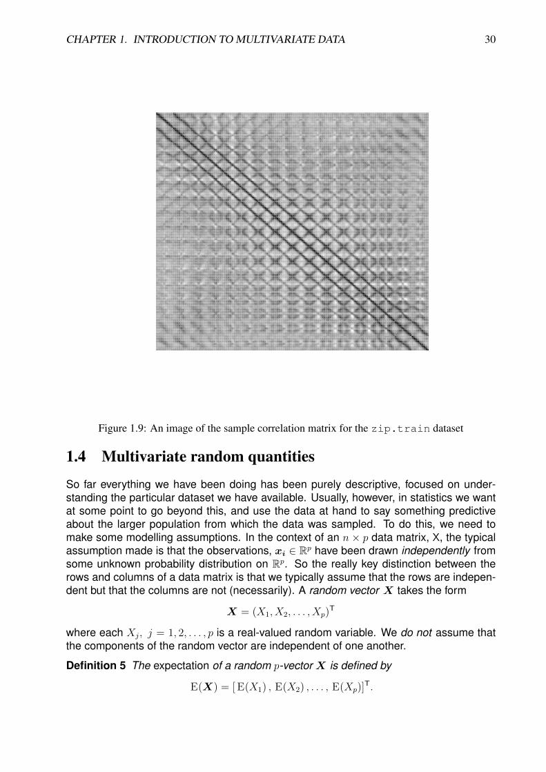
CHAPTER 1. INTRODUCTION TO MULTIVARIATE DATA 30
Figure 1.9: An image of the sample correlation matrix for the zip.train dataset
1.4 Multivariate random quantities
So far everything we have been doing has been purely descriptive, focused on under-standing the particular dataset we have available. Usually, however, in statistics we wantat some point to go beyond this, and use the data at hand to say something predictiveabout the larger population from which the data was sampled. To do this, we need tomake some modelling assumptions. In the context of an n × p data matrix, X, the typicalassumption made is that the observations, xi ∈ Rp have been drawn independently fromsome unknown probability distribution on Rp. So the really key distinction between therows and columns of a data matrix is that we typically assume that the rows are indepen-dent but that the columns are not (necessarily). A random vector X takes the form
X = (X1, X2, . . . , Xp)T
where each Xj, j = 1, 2, . . . , p is a real-valued random variable. We do not assume thatthe components of the random vector are independent of one another.
Definition 5 The expectation of a random p-vector X is defined by
E(X) = [ E(X1) , E(X2) , . . . , E(Xp)]T.
CHAPTER 1. INTRODUCTION TO MULTIVARIATE DATA 31
So, the expectation of a random vector is just defined to be the vector of expected values.Similarly, the expected value of a random matrix is the matrix of expected values. Also, ifwe recall that the covariance between two scalar random variables X and Y is defined by
Cov(X, Y ) = E([X − E(X)][Y − E(Y )])
(so for independent X, Y we will have Cov(X, Y ) = 0), we see that the variance matrix fora random matrix is defined to be the matrix of covariances between pairs of elements:
Definition 6 The variance matrix of a random p-vector X is defined by
Var(X) = E([X − E(X)][X − E(X)]T
).
Example: toy problem
Suppose that X = (X1, X2)T, where X1 ∼ Exp(1) and X2 ∼ Exp(2) are independent
random quantities. What is E(X) and Var(X)?
Calculating everything required one component at a time,we have E(X1) = 1, Var(X1) = 1, E(X2) = 1/2, Var(X2) =
1/4, and since the variables are independent, we must haveCov(X1, X2) = 0, giving
E(X) =
(1
1/2
), Var(X) =
(1 0
0 1/4
).
We will show later that in some appropriate sense, if we regard a multivariate datasetX as a random sample from a multivariate distribution, then it turns out that the samplemean of X is a “good” estimator of E(X), and similarly, the sample variance matrix, S, isa “good” estimator of Var(X).
1.5 Transformation and manipulation of multivariate randomquantities and data
When working with multivariate random quantities and data, we often want to transformthem in some way in order to highlight some aspect of interest, or reduce dimension, etc.We have already seen some examples of transformations applied to multivariate data.Subsetting columns from a data matrix is a particularly simple example, and formally canbe regarded as a projection into a lower dimensional space. In particular, picking out twocolumns in order to produce a scatter-plot is an example of a projection of the data intoa 2-dimensional space. The centering matrix was another example of a transformation ofthe data matrix, corresponding to subtraction of the mean. These simple examples areall examples of affine transformations, and so it will be helpful to remind ourselves of thebasic idea behind affine transformations before proceeding to see how we can use themto transform random vectors and multivariate data.

CHAPTER 1. INTRODUCTION TO MULTIVARIATE DATA 32
1.5.1 Linear and affine transformations
In Euclidean space a linear transformation (or linear map) is represented by a real-valuedmatrix. For example, the map
f : Rp −→ Rq
will have matrix representationf(x) = Ax
for some q×p matrix A. In the context of multivariate statistics we would expect that q ≤ p,so that the map will either preserve the dimension of the original space q = p, or projectthe data into a lower dimensional space q < p. Since it is clear that
f(ej) = Aej = a(j),
the jth column of A, we can form A by considering the destination of ej, j = 1, 2, . . . , p inthe new space, Rq.
An important special case arises in the case q = 1, so that the map is real valued, andrepresents a linear functional. Linear functionals can be represented with a p-vector, a,as
f(x) = aTx.
It turns out that in many applications in multivariate statistics, we want to combine a lineartransformation with a shift in location. Such maps are referred to as affine transformations,and the affine map
f : Rp −→ Rq
can be represented asf(x) = Ax+ b,
for some q × p matrix A and q-vector b. Note that f(0) = b, so that b can be identified asthe image of 0, and then
f(ej) = a(j) + b,
and hence the columns of A are determined by
a(j) = f(ej)− b.
Note that affine transformations can be represented with a single (q + 1)× (p + 1) matrixof the form
A =
(A b0T 1
)by augmenting the vectors in both spaces with a “1”, since then(
y
1
)= A
(x
1
)=
(A b0T 1
)(x
1
)=
(Ax+ b
1
),
CHAPTER 1. INTRODUCTION TO MULTIVARIATE DATA 33
and is therefore equivalent toy = Ax+ b.
This technique of representing an affine transformation as a linear transformation in anaugmented space makes it convenient to combine multiple affine transformations (viamatrix multiplication), and is used extensively in computer graphics.
Example: linear combination
The linear combination of variables
y = a1x1 + a2x2 + · · ·+ apxp + b
can be represented as the affine transformation
y = aTx+ b.
Example: 2d projection
We may view the selection of variables to plot in one window of a scatterplot matrix as a2d projection of the multivariate data. Selection of components xk and xj corresponds tothe projection
y =
(ek
T
ejT
)x,
and hence the linear transformation with A = (ek, ej)T.
More generally, we can project onto the linear subspace spanned by any two orthogo-nal unit p-vectors, v1, v2 using
A = (v1,v2)T.
This follows since we can write x as
x = y1v1 + y2v2 +w,
where w is orthogonal to v1 and v2. From this it follows that vi · x = yi, and the resultfollows. Note that, as above, A has the property AAT = I2. 2d projections are obviouslyvery useful for visualisation of high-dimensional data on a computer screen.
1.5.2 Transforming multivariate random quantities
We can apply an affine transformation to a random p-vector X to get a random q-vectorY . It is natural to wonder how the expectation and variance of Y relate to that of X.
Proposition 7 Let X be a random p-vector with expectation vector E(X) and variancematrix Var(X). Consider an affine transformation of X from Rp to Rq given by
Y = AX + b,
where A is a q × p matrix and b is a q-vector. Then the expectation and variance of Y aregiven by
E(Y ) = A E(X) + b, Var(Y ) = A Var(X) AT.

CHAPTER 1. INTRODUCTION TO MULTIVARIATE DATA 34
ProofFirst consider E(Y ),
E(Y ) = E(AX + b)
= E
a11 a12 · · · a1p
... ... . . . ...aq1 aq2 · · · aqp
X1
X2...Xp
+
b1...bq
= E
a11X1 + a12X2 + · · · + a1pXp + b1...
aq1X1 + aq2X2 + · · · + aqpXp + bq
=
E(a11X1 + a12X2 + · · · + a1pXp + b1)...
E(aq1X1 + aq2X2 + · · · + aqpXp + bq)
=
a11 E(X1) + a12 E(X2) + · · · + a1p E(Xp) + b1...
aq1 E(X1) + aq2 E(X2) + · · · + aqp E(Xp) + bq
= A E(X) + b.
Once we have established linearity of expectation for vector random quantities, thevariance result is relatively straightforward.
Var(Y ) = E([Y − E(Y )][Y − E(Y )]T
)= E
([AX + b− A E(X)− b][AX + b− A E(X)− b]T
)= E
([AX − A E(X)][AX − A E(X)]T
)= E
(A[X − E(X)][X − E(X)]TAT
)= A E
([X − E(X)][X − E(X)]T
)AT
= A Var(X) AT

CHAPTER 1. INTRODUCTION TO MULTIVARIATE DATA 35
�
We are now in a position to establish that the variance matrix of a random vectorshares two important properties with sample covariance matrices.
Proposition 8 The variance matrix, Var(X) is symmetric and positive semi-definite.
Proof
Var(X) T = {E([X − E(X)][X − E(X)]T
)}T
= E({[X − E(X)][X − E(X)]T}T
)= E
([X − E(X)][X − E(X)]T
)= Var(X) .
Similarly, for any p-vector α we have
αT Var(X)α = αT E([X − E(X)][X − E(X)]T
)α
= E(αT[X − E(X)][X − E(X)]Tα
)= E
({[X − E(X)]Tα}2
)≥ 0,
since non-negative random scalars cannot have negative ex-pectation.
�
Example: mean and variance of a linear combination
The special case of linear functionals of random quantities turns out to be very important.So consider the random (scalar) variable Y defined by
Y = αTX + b
where α is a given fixed p-vector and b is a fixed scalar. From our above results it is clearthat
E(Y ) = αT E(X) + b
andVar(Y ) = αT Var(X)α.
Importantly, we note that the positive semi-definiteness of Var(X) corresponds to the factthat there are no linear combinations of X with negative variance.

CHAPTER 1. INTRODUCTION TO MULTIVARIATE DATA 36
Example: toy problem
Suppose that X = (X1, X2, X3)T, where the components Xi ∼ Po(i), i = 1, 2, 3 are
mutually independent. Consider
Y =
(1 2 34 5 6
)X +
(0
1
).
What are E(Y ) and Var(Y )?
We first need to know that
E(X) =
1
2
3
and Var(X) =
1 0 0
0 2 0
0 0 3
.
The we can calculate
E(Y ) =
(1 2 3
4 5 6
)1
2
3
+
(0
1
)=
(14
32
)+
(0
1
)=
(14
33
),
and
Var(Y ) =
(1 2 3
4 5 6
)1 0 0
0 2 0
0 0 3
1 4
2 5
3 6
=
(1 2 3
4 5 6
)1 4
4 10
9 18
=
(36 78
78 174
).
Example: transforming standard random vectors
Suppose that we start with a random p-vector Z where the components are mutuallyindependent with zero expectation and variance 1. Now consider a p-vector Y where
Y = AZ + µ,
where A is a p× p matrix and µ is a p-vector. What is E(Y ) and Var(Y )?
CHAPTER 1. INTRODUCTION TO MULTIVARIATE DATA 37
We first note that E(Z) = 0 and Var(Z) = Ip, and then compute
E(Y ) = A E(Z) + µ = µ
andVar(Y ) = A Var(Z) AT = A Ip AT = AAT.
Notes:
1. Suppose we would like to be able to simulate random quantities with a given ex-pectation µ and variance Σ. The above transformation provides a recipe to do so,provided that we can simulate iid random quantities with mean zero and varianceone, and we have a method to find a matrix A such that AAT = Σ. We will examinetechniques for factorising Σ in the next chapter.
2. The special case where the elements of Z are iid N(0, 1) is of particular importance,as then Y is said to have a multivariate normal distribution. We will investigate thiscase in more detail later.
1.5.3 Transforming multivariate data
We can apply an affine transformation to each observation of a data matrix, X. Conceptu-ally, we do this by transposing the data matrix to get column vectors of observations, thenpre-multiply by A, then add b to each column in order to get the transpose of the new datamatrix, Y. In other words
Y = (AXT + b11nT)T,
leading to
Proposition 9 The affine transformation from Rp to Rq given by
y = Ax+ b
can be applied to an n× p data matrix X to get a new n× q data matrix Y given by
Y = XAT + 11nbT.
Again, we would like to know how the sample mean, y and variance SY of the new datamatrix Y relate to the sample mean x and variance matrix SX of X.
Proposition 10 The sample mean and variance of Y are related to the sample mean andvariance of X by
y = Ax+ b, SY = ASXAT.
ProofLet’s start with the sample mean,

CHAPTER 1. INTRODUCTION TO MULTIVARIATE DATA 38
y =1
nYT11n
=1
n(XAT + 11nb
T)T11n
=1
n(AXT11n + b11n
T11n)
=1
nAXT11 + b
= Ax + b.
The sample variance matrix result is left as an exercise.�
Example: Galaxy data
First let’s return to the galaxy data, and just extract two columns:
sub=galaxy[c("radial.position","velocity")]
This is clearly a projection into a 2d space, but there is no point in explicitly constructingthe linear transformation. We can then center the data. This is also an affine transforma-tion, which we can construct and then plot with
subCentered=sweep(sub,2,colMeans(sub))plot(subCentered,col=galaxy$angle,pch=19)
giving the figure shown in Figure 1.10.Now suppose that we would like to apply a further transformation to this data, namely
rotation anti-clockwise through 10 degrees (π/18 radians). We know from elementarygeometry that this can be accomplished as a linear transformation with matrix
A =
(cos θ − sin θsin θ cos θ
),
where θ = π/18. We can then apply this transformation to the data matrix and re-plot with
A=matrix(c(cos(pi/18),-sin(pi/18),sin(pi/18),cos(pi/18)),ncol=2,byrow=TRUE)
subRotated=as.matrix(subCentered) %*% t(A)plot(subRotated,col=galaxy$angle,pch=19)
giving the plot shown in Figure 1.11.
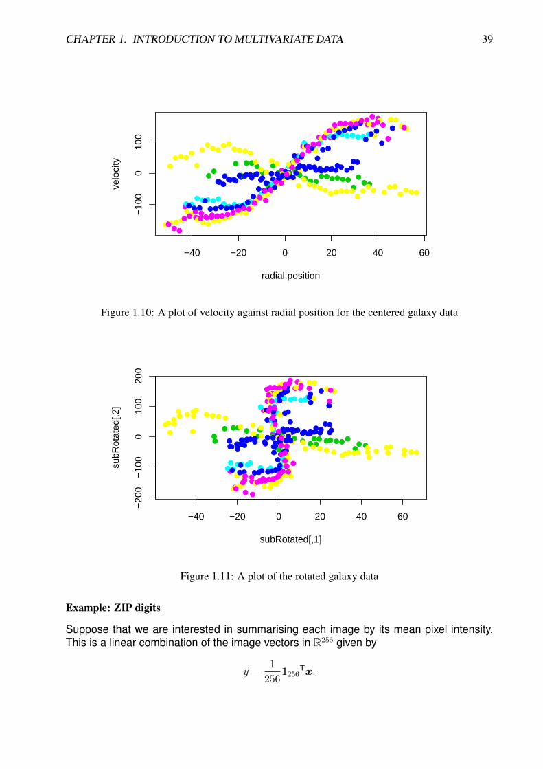
CHAPTER 1. INTRODUCTION TO MULTIVARIATE DATA 39
●●●●●●●●
●
●●●
●●●
●●
●●
●●
●●
●●●
●●
●●●●●●
●
●
●
●●
●●●●●●●
●
●●●●
●●
●●●●
●●●
●
●●●●●●●●●●
●●
●
●●
●
●●●
●●
●●●●●●●●●●●●
●●
●●●●●
●
●●●●
●●●●●
●
●●●
●
●●
●●
●●●
●
●●●●
●●●●●●
●●●
●●●●
●●●
●
●●●●●●●●●
●●
●●●
●
●
●●
●●
●
●
●●
●
●
●●
●
●●●●●
●
●●
●
●●
●
●●
●●
●●●●
●●
●●●●●●●
●
●●●
●●●●
●●●●
●●
●●●●●●
●●●●●
●
●●●
●●
●●
●
●●●●●●
●●●
●
●
●●●●
●●
●●●
●●●●●●●●
●●●●●
●●
●●●●●●
●●
●
●
●●●
●●●●●●●
●●
●●●
●●
●●
●●
●●●
●●●●●●●●●●●
●●●
●●●
−40 −20 0 20 40 60
−10
00
100
radial.position
velo
city
Figure 1.10: A plot of velocity against radial position for the centered galaxy data
●●●●●●●●
●
●●●
●●●
●●
●●
●●
●●
●●●●●●●●●●
●●
●
●
●●●●●●●●
●
●
●●●●
●●
●●●●
●●●●
●●●●●●●●●●
●●
●
●●●
●●●●●●●●●●●●
●●●●●●●
●●●●●
●
●●●●
●●●●●●
●●●
●
●●
●●●●●
●
●●●●
●●●●●●
●●●
●●●●
●●●
●●●●●●●
●●●●
●●●
●●
●
●●
●●
●
●
●●
●
●
●●●
●●●●●
●
●●
●
●●
●
●●
●●
●●●●
●●●●●●●●●
●●●●
●●●●
●●●●
●●●
●●●●●●●●●
●●
●●●
●●
●●●
●●●●●●
●●●●
●
●●●●
●
●●●
●●●●●●●●●
●●●●●
●●
●●●●●●
●●
●
●
●●●●●
●●●●●●●●●●
●●
●●
●●
●●●●●●●●●●●●●●
●●●
●●●
−40 −20 0 20 40 60
−20
0−
100
010
020
0
subRotated[,1]
subR
otat
ed[,2
]
Figure 1.11: A plot of the rotated galaxy data
Example: ZIP digits
Suppose that we are interested in summarising each image by its mean pixel intensity.This is a linear combination of the image vectors in R256 given by
y =1
25611256
Tx.
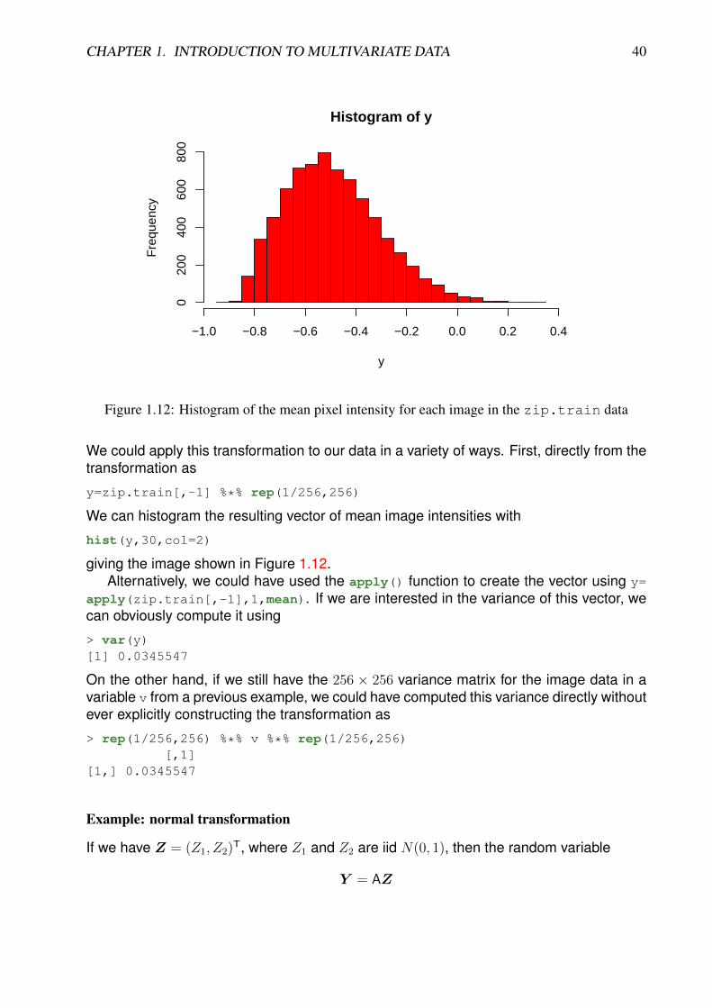
CHAPTER 1. INTRODUCTION TO MULTIVARIATE DATA 40
Histogram of y
y
Fre
quen
cy
−1.0 −0.8 −0.6 −0.4 −0.2 0.0 0.2 0.4
020
040
060
080
0
Figure 1.12: Histogram of the mean pixel intensity for each image in the zip.train data
We could apply this transformation to our data in a variety of ways. First, directly from thetransformation as
y=zip.train[,-1] %*% rep(1/256,256)
We can histogram the resulting vector of mean image intensities with
hist(y,30,col=2)
giving the image shown in Figure 1.12.Alternatively, we could have used the apply() function to create the vector using y=
apply(zip.train[,-1],1,mean). If we are interested in the variance of this vector, wecan obviously compute it using
> var(y)[1] 0.0345547
On the other hand, if we still have the 256 × 256 variance matrix for the image data in avariable v from a previous example, we could have computed this variance directly withoutever explicitly constructing the transformation as
> rep(1/256,256) %*% v %*% rep(1/256,256)[,1]
[1,] 0.0345547
Example: normal transformation
If we have Z = (Z1, Z2)T, where Z1 and Z2 are iid N(0, 1), then the random variable
Y = AZ
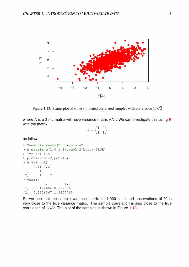
CHAPTER 1. INTRODUCTION TO MULTIVARIATE DATA 41
●
●●
●
●
●
●●
●
●
●●
●●
●
●●
●
●●
●
●
●
●
●
●
●
●
●
●
●
●
●
●
●
●
●
●
●
●
●
●
●
●
●
● ●
●●
●
●●
●●
●●
●● ●
●
●●
●●
●
●
●●
●
●
●
●● ●
●
●
●
●
●
●
●
●
●
●
● ●●●
●
●
●
●●
●
●
●
●●
●
●
●● ●
● ●
●
●
●
●
●
●●
● ●
●
●
●
●
●
●
●●
●
●●
●●
●
●
●
●
●
●●●
●
●
●
●
●
●
●●
●●●
●●
●
●●
●
●
●
●
●
●
●
● ●●
●● ●
●
●●
●
●
●●
●
●
●●
●
●
●
●●
●
●●
●
●●
●
●
●
●
● ●
●
●
●
●
●●
●
●
●
●
●
●
●
●
● ●
●●
●
●
●●
●
●
●
●
● ●
●
●
●
●
●
●
●
●
●
●●
●●
●
●
●
●● ●
●
●●
●
●
●
●
●
●
●
●●
●
●
●
●
●
●●
●
●
●
●●
●
●
●
●
●●
●
●
●●
●
●
●●
● ●●
●
● ●
●
●
●
●
●
●
●
●
●●
●●●
●
●
● ●
●
●●
●●
●●
●
●
●
●
●●
●
●●
●
●●
●
●●●
●
●● ●●
●●
●
●
●
●
●
●
●
●● ●
●●
●
●
●
●
●●
●
● ●● ●
●
●
● ●
●
●
●
●●
●
●
●
●
●
●●
●
●
● ●
●
●
●●
●
●
●
●
●
●
●
●
●
● ●●
●
●
●
●
●
●
●
●●
●
●
●
●
●●
●
●
●
●
●
●
●●
●
●●
●
●
●
●
●
●
●
●●
●
●●
● ●
●
●
●
●● ●
●
●
●
●
● ●●
●●
●
● ●
●
●
●
●
●
●●
●
●
●
●
●●
●
●
●●
●
●
●●
●●
●
●●
●
●
●●●
●
●●
●
●
●
●
●●
●
●●
●
●
●
●●
●
●
●
●
●●
●
●●
●●
●
●
●●
●
● ●
●
●
●
●●
●
●●
●
●
●●
●
●
●
●
●●
●
●
●●
●
●
●
●●
●●
●
●
●●
●
●
●●
●
●
●
●
●
●
●
●
●
●●
●
●
●●
●●
●
●●
●
●
●
●●●
●●
●
●
●
●
●
●
●
●
●
●
●●●
●
●
●●●
●
●
●● ●
●
●
●
●
●
●
●●
●
●
●
●
●
●
●
●●
●●
●
●●
●
●
●
●
●
●●
●
●
●
●
●
●
●
●●
●
●●
●
●
● ●
●
●
●
●
●
●
●
●●
●
●
●
●
●
●
●
●
●
●
●
●
●●
●
●●● ●
●●
●●
●
●
●
●
●
●
●
● ●●●
●
●
●
●
●
●
●
●
●●
●●
●
●
●
●●
● ●●
●
● ●
●
●
●
●
●
●
●
●
●
●●
●
●
●●
●
●
●●
●●
●●
●
●
● ●
●
●
●
●
●
●
●
●
●
●
●
●●
●●●
●
●
●
●●
●
●
●
●
●
●
●●
●
●
●●
●
●
●
●●
●
●●●
●
●●
●
●
●
●
●
●
●●●
●
●
●
●
●●
●
●
●
●
●
●
●
●
●
●
●
●
●
●
●
●●
●●●
●
●
●
●●
●
●
●
●
●
●●
●
●
●
●
●
●
●
●
●
●
● ●●●
●
●
●●
●
●
●●
●
●
●
●
●●
●
●●
●
●
●
●
●
●●
●
●●
●
●
●
●
●
●
●●
●
●
●
●
● ●●
●
●
●
●
●
●
●
●
●
●
●
●
●
●
●
●●
● ●●
●
●
●
●
●
●●
●
●
●
●
●
●●
●
●
●●
●
● ●●
●
●
● ●
●
● ●●
●
●
●●
●
● ●
●
●●
●
●
●
●
●
●
●
●●
●
●●
●
●
●
●
● ●
●
●
●
●
● ●
●
●
●
● ●
●
●
●
●
●
●
●
●
●
●
●
●
● ●
●●●
●
●
●
● ●
●
●
−4 −3 −2 −1 0 1 2 3
−4
−2
02
4
Y[,1]
Y[,2
]
Figure 1.13: Scatterplot of some simulated correlated samples with correlation 1/√
2
where A is a 2 × 2 matrix will have variance matrix AAT. We can investigate this using Rwith the matrix
A =
(1 01 1
)as follows
> Z=matrix(rnorm(2000),ncol=2)> A=matrix(c(1,0,1,1),ncol=2,byrow=TRUE)> Y=Z %*% t(A)> plot(Y,col=2,pch=19)> A %*% t(A)
[,1] [,2][1,] 1 1[2,] 1 2> var(Y)
[,1] [,2][1,] 1.0194604 0.9926367[2,] 0.9926367 1.9257760
So we see that the sample variance matrix for 1,000 simulated observations of Y isvery close to the true variance matrix. The sample correlation is also close to the truecorrelation of 1/
√2. The plot of the samples is shown in Figure 1.13.

CHAPTER 1. INTRODUCTION TO MULTIVARIATE DATA 42
Example: toy example
Consider the following data matrix with n = 4 and p = 3:
X =
1 2 32 3 43 2 11 3 2
.
Suppose that we wish to construct a new data matrix Y based on the affine transformation
y =
(1 1 00 0 1
)x+
(0
1
).
Construct the 4× 2 data matrix Y.
Y =
1 2 3
2 3 4
3 2 1
1 3 2
1 0
1 0
0 1
+
0 1
0 1
0 1
0 1
=
3 3
5 4
5 1
4 2
+
0 1
0 1
0 1
0 1
=
3 4
5 5
5 2
4 3
.
When we introduced affine transformations, we discussed the augmented form of thetransformation, where the vector to be transformed was augmented with a “1” so that theaffine map could be accomplished as a linear transformation. If we wish, we can usethis method on a data matrix, X, by augmenting it with a column of “1”s. Then the keytransformation equation is
(Y, 11n) = (X, 11n)
(AT 0bT 1
).
Note that this is very much analogous to prepending the design matrix with a column of“1”s in multiple linear regression, in order to avoid explicit consideration of an interceptterm.

CHAPTER 1. INTRODUCTION TO MULTIVARIATE DATA 43
We now have all of the basic skills we need to be able to begin to think about moresophisticated methods of multivariate data analysis. See Chapter 1 of [HTF] and Chapters1 and 2 of [Everitt] for further background and details relating to the material in thischapter.
Chapter 2
PCA and matrix factorisations
2.1 Introduction
2.1.1 Factorisation, inversion and linear systems
It should be clear by now that linear algebra and matrix computations are central to mul-tivariate statistics. For the analysis of large and complex datasets it is essential to havea basic knowledge of computational linear algebra, and this starts with an understandingof the efficient solution of linear systems, and the role of various different matrix factori-sations, often known as matrix decompositions, to transform general linear systems intovery special linear systems that are much easier to solve.
We have already seen a couple of instances of matrix factorisation. First, we showedthat the sample covariance matrix, S, could be decomposed as
S = ATA
for some matrix A. We were able to use this fact to deduce important properties of S.Similarly, we showed that applying a matrix A to a vector of independent random quantitieswith unit variance resulted in a vector with covariance matrix AAT. We noted that if wewere interested in simulating random quantities with a given covariance matrix Σ, wecould do this if we were able to find a matrix A such that
Σ = AAT.
This would be an example of a matrix factorisation, or matrix decomposition. Unsurpris-ingly, there is not a unique solution to this factorisation problem, but in this chapter wewill see how to construct two different factorisations of Σ which both provide an effectivesolution to this problem.
The solution of linear systems will also turn out to be a recurring theme. That is,solving equations of the form
Ax = b
for x, given a specific matrix A and vector b. We know that in principle, if A is invertible,the unique solution is given by
x = A−1b.
However, it turns out that solving the problem directly in this way, by first computing A−1
and then pre-multiplying b by this matrix is a very inefficient and numerically unstable way
44

CHAPTER 2. PCA AND MATRIX FACTORISATIONS 45
to approach the problem. It is hardly ever necessary to directly compute the inverse ofa matrix. There are usually far more efficient ways to solve a linear system, sometimesby solving the linear system directly (say, using Gaussian elimination), or more usually bysolving in multiple steps using matrix factorisations. By way of motivation, suppose thatwe have an efficient way to factorise A as
A = LU,
where L and U are lower and upper triangular matrices, respectively.∗ We can then solveAx = b by writing the problem as
LUx = b.
If we define v = Ux, we can first solve
Lv = b
for v and then solveUx = v
for x. It turns out that triangular linear systems are very easy to solve, so solving two trian-gular linear systems is much faster than solving one general linear system. To progressfurther we need to know more about triangular matrices, linear systems, and factorisa-tions.
2.2 Triangular matrices
2.2.1 Upper and lower triangular matrices
It is possible to develop a theory of triangular matrices and triangular matrix factorisationfor non-square matrices, but for the purposes of this course this is unnecessary, so wewill restrict ourselves to thinking about square matrices.
Definition 7 An n× n matrix A is lower triangular if all elements above the leading diag-onal are zero, that is aij = 0, ∀j > i. Similarly, a matrix is upper triangular if all elementsbelow the leading diagonal are zero, that is aij = 0, ∀i > j.
Clearly only diagonal matrices are both upper and lower triangular. Upper and lowertriangular matrices have very similar properties (since one is just a transpose of the other).We will focus mainly on lower triangular matrices. It should be assumed that there areexactly analogous properties for upper triangular matrices unless otherwise stated.
Proposition 11 1. The sum of two lower triangular matrices is also lower triangular
2. The product of two lower triangular matrices is also lower triangular
3. If a lower triangular matrix is invertible, the inverse is also lower triangular
4. The determinant of a lower triangular matrix is the product of the diagonal elements∗We will explain what this means in the next section. For now it suffices to know that they are just special matrices.

CHAPTER 2. PCA AND MATRIX FACTORISATIONS 46
5. A lower triangular matrix is invertible iff all diagonal elements are non-zero
6. The eigenvalues of a lower triangular matrix are the diagonal elements of the matrix
Proof
1. Clear from definition
2. Left as an exercise
3. Thinking about using the Gaussian elimination method to construct this inverse, it isclear that it will only be necessary to use row operations which are lower triangular,leading to a lower triangular inverse
4. Direct expansion of the determinant along the top row in terms of minor determi-nants, applied recursively, makes this clear
5. The determinant will be non-zero iff all diagonal elements are non-zero, by previousresult
6. The eigenvalues are given by the roots of |A − λ I |. This matrix is lower triangular,so the determinant is the product of diagonal elements.
�
2.2.2 Unit triangular matrices
Definition 8 A matrix L is unit lower triangular if it is lower triangular, and has the addi-tional property that all elements along the leading diagonal are 1, that is, lii = 1, ∀i.
In addition to all of the properties of lower triangular matrices, unit lower triangular matri-ces have some additional useful properties.
Proposition 12 1. The product of two unit lower triangular matrices is unit lower trian-gular
2. The inverse of a unit lower triangular matrix is unit lower triangular
3. The determinant of a unit lower triangular matrix is 1, and hence all unit lower trian-gular matrices are invertible
4. The eigenvalues of a unit lower triangular matrix are all equal to 1
Proof
1. Left as an exercise
2. Again, clear by thinking about Gaussian elimination and row operations
3. The determinant is the product of the diagonal elements
4. |L− λ I | = (1− λ)n.

CHAPTER 2. PCA AND MATRIX FACTORISATIONS 47
�
It is clear that a non-singular lower triangular matrix A can be factorised in the form
A = DL
where D is diagonal and L is unit lower triangular, by choosing D = diag {a11, a22, . . . , ann}and L = D−1A.
Example: Toy problem
Write the 2× 2 lower triangular matrix
A =
(2 0−1 4
)in the form A = DL, where D is diagonal and L is unit lower triangular.
If we put
D = diag {2, 4} , D−1 = diag {1/2, 1/4}
we get
L = D−1A =
(1/2 0
0 1/4
)(2 0
−1 4
)=
(1 0
−1/4 1
)and we are done. The resulting factorisation is(
2 0
−1 4
)=
(2 0
0 4
)(1 0
−1/4 1
).
2.2.3 Forward and backward substitution
One of the main reasons for thinking specifically about triangular matrices is that triangularlinear systems turn out to be rather easy to solve. Consider the lower triangular equation
Lx = b,
where n × n L and n-dimensional b are given, and a solution for n-dimensional x is re-quired. We will assume that L is invertible (no zeros on the diagonal), so that the solutionis unique. If we re-write the equation in component form, a simple solution strategy be-comes apparent:
l11 0 · · · 0l21 l22 · · · 0...
... . . . ...ln1 ln2 · · · lnn
x1x2...xn
=
b1b2...bn
.

CHAPTER 2. PCA AND MATRIX FACTORISATIONS 48
We can see that the first equation is just
l11x1 = b1 ⇒ x1 = b1/l11.
But now we can use x1 to solve the second equation as
l21x1 + l22x2 = b2 ⇒ x2 = (b2 − l21x1)/l22.
In general we can solve for xi in terms of x1, . . . , xi−1 as
xi =
(bi −
i−1∑j=1
lijxj
)/lii.
Iterative construction of the solution in this way is known as forward substitution. Clearlythe algorithm would fail if any lii = 0, but this corresponds to the rank degenerate case.For the invertible case we are considering, the algorithm provides a simple and efficientmethod for computing a solution.
Example: Toy problem
Solve the triangular system (2 01 4
)x =
(4
6
)for x. (
2 0
1 4
)(x1
x2
)=
(4
6
),
so, starting with the first equation we have
2x1 = 4⇒ x1 = 2.
The second equation can then be solved as
x1 + 4x2 = 6⇒ x2 =6− x1
4=
6− 2
4= 1,
so our solution is x = (2, 1)T.
Example: forward solve using R
Use R to solve the system 2 0 01 3 02 3 4
x =
6928
for x.
This is easily accomplished as shown in the following R session

CHAPTER 2. PCA AND MATRIX FACTORISATIONS 49
> L=matrix(c(2,0,0,1,3,0,2,3,4),ncol=3,byrow=TRUE)> L
[,1] [,2] [,3][1,] 2 0 0[2,] 1 3 0[3,] 2 3 4> forwardsolve(L,c(6,9,28))[1] 3 2 4>
The solution is therefore given by x = (3, 2, 4)T.The solution of upper triangular systems is analogous, but looks a little different, so
we will consider it explicitly. Suppose that U is an upper triangular matrix, and we want tosolve the system
Ux = b
for x. Again, we write out the system in component form:u11 u12 · · · u1n0 u22 · · · u2n...
... . . . ...0 0 · · · unn
x1x2...xn
=
b1b2...bn
.
We now see that system is easiest to solve starting with the last equation
unnxn = bn ⇒ xn = bn/unn,
thenun−1,n−1xn−1 + u(n−1),nxn = bn−1 ⇒ xn−1 = (bn−1 − u(n−1),nxn)/un−1,n−1,
and so on, with xi given by
xi =
(bi −
n∑j=i+1
uijxj
)/uii.
This procedure is known as backward substitution, for obvious reasons.
Example: backward solve using R
Solve the upper triangular system2 2 30 2 −10 0 3
x =
86−6
for x using R.
This is easily accomplished as the following R session shows
> R=matrix(c(2,2,3,0,2,-1,0,0,3),ncol=3,byrow=TRUE)> R
[,1] [,2] [,3]

CHAPTER 2. PCA AND MATRIX FACTORISATIONS 50
[1,] 2 2 3[2,] 0 2 -1[3,] 0 0 3> backsolve(R,c(8,6,-6))[1] 5 2 -2
So the solution is x = (5, 2,−2)T.
2.3 Triangular matrix decompositions
2.3.1 LU decomposition
We now know how to solve triangular systems of equations, but most linear systemsof interest do not start out in triangular form. However, as already outlined, if we canfactorise or decompose a system into triangular components, we can solve a sequenceof triangular systems in order to get a solution to our original problem. The problem wewill consider now is the following.
Proposition 13 (LU decomposition) Given a non-singular n × n matrix A, we can findunit lower triangular L and upper triangular U such that
A = LU.
Clearly then, since |A| = |LU| = |L||U| = |U|, we have |A| =∏n
i=1 uii, and this is an efficientway to compute the determinant in the rare cases where it is really needed.
The factorisation is just a matrix representation of the procedure of using Gaussianelimination to zero out the lower triangle of A to create U. L represents the (inverse ofthe) row operations required to achieve this. We will not give a formal derivation of theconstruction, but instead give a rough outline. First we note that the row operations usedin Gaussian elimination can be represented by matrices. So the row operation which addsλ times row i to row j can be represented by the matrix
Mij(λ) = I +λejeiT,
and λ is known as the multiplier of the operation. The row operations needed to zero outthe lower diagonal will all have i < j, so Mij(λ) will be unit lower triangular, and thereforethe product of all of the row operations will also be unit lower triangular. Row operationsare easily inverted, as
Mij(λ)−1 = I − λejeiT.
This can be verified by multiplication, noting particularly how the final product term van-ishes. It will require n(n − 1)/2 such row operations to zero out the lower triangle. Ifwe number them sequentially, so that M1 is the row operation to zero out a21, M2 is therow operation to zero out a31, etc., then the matrix representing the complete set of rowoperations is
M = Mn(n−1)/2 · · ·M2M1.
Then if we denote the upper triangle that we are left with by U we have
MA = U⇒ A = M−1U = LU

CHAPTER 2. PCA AND MATRIX FACTORISATIONS 51
where L = M−1. NowL = M1
−1M2−1 · · ·Mn(n−1)/2
−1,
and the individual terms of this product are all trivial to write down. Remarkably, the unitlower triangular product is also trivial to compute. It turns out to be simply the unit lowertriangular matrix whose off-diagonal elements are (minus) the row operation multipliersused to zero out that entry. Note that this is due to all of the product terms cancelling,and this in turn depends crucially on the order in which the operations are applied. Theproduct terms cancel in the inverse L and not in M because in the inverse, no new rowoperation is introduced which uses a row that has already been modified as the “source”for a new row operation. The factorisation procedure is best illustrated by example.
Example: toy problem
Let A be the 3× 3 matrix
A =
1 4 72 5 83 6 10
.
Find the LU decomposition of A.
Start with
A =
1 4 7
2 5 8
3 6 10
and zero out the first column. The required multipliers are -2and -3 respectively, so we record their “inverses”, 2 and 3, inthe locations we have zeroed out:1 4 7
2 −3 −6
3 −6 −11
.
Now we zero out the second column with the multiplier -2, andso we record the number 2 in the position we zero out:1 4 7
2 −3 −6
3 2 1
.
CHAPTER 2. PCA AND MATRIX FACTORISATIONS 52
That’s it! The LU factorisation is
A =
1 4 7
2 5 8
3 6 10
=
1 0 0
2 1 0
3 2 1
1 4 7
0 −3 −6
0 0 1
.
2.3.2 LDMT decomposition
The LU factorisation has U upper triangular and L unit lower triangular. We have alreadyseen that we can factorise non-singular U as U = DR where D is diagonal and R is unitupper triangular, and this leads directly to the LDMT decomposition of a non-singularmatrix A as
A = LDMT,
where L and M = RT are unit lower triangular, and D is diagonal. It is clear from thisdecomposition that |A| = |LDMT| = |L||D||MT| = |D| =
∏ni=1 dii. We can obviously con-
struct this decomposition from the LU factorisation of A. It turns out that there is also adirect construction which is slightly more efficient, but this is not especially relevant in thecontext of this course.
2.3.3 LDLT decomposition
In many statistical applications, the matrix A we want to factorise is symmetric (for exam-ple, it is often a covariance or correlation matrix). In this case it turns out that the LDMT
decomposition takes the form LDLT, that is L = M. In some sense this is obvious, andis certainly intuitive, as it has the same form as the LDMT decomposition, and is clearlysymmetric. However, it is not completely obvious that the LDMT decomposition has to beof this form, but it has.Proposition 14 The LDMT decomposition of a non-singular symmetric matrix A has L =M, giving the decomposition
A = LDLT,
where L is unit lower triangular and D is diagonal.Proof
Start with A = LDMT, and first post-multiply by M−T and then pre-multiply by M−1 toget
M−1AM−T = M−1LD.
The LHS of this equation is clearly symmetric, and the RHS is clearly lower triangular.Therefore both sides must be diagonal. But if M−1LD is diagonal, M−1L must also be. Butthis is also clearly unit lower triangular, so must be the identity. That is, M−1L = I, andhence M = L. �
The symmetry in this factorisation opens up the possibility of developing more efficientalgorithms for constructing the decomposition, rather than starting with a basic LU de-composition. Rather than examine such strategies for this particular factorisation, wewill do so in the context of a very closely related decomposition, usually known as theCholesky decomposition.
CHAPTER 2. PCA AND MATRIX FACTORISATIONS 53
2.3.4 The Cholesky decomposition
If the symmetric matrix A is not only non-singular, but also positive definite, then we canconstruct another factorisation that is very widely used in statistical applications. We willfirst construct it from the LDLT decomposition, but then derive a more direct and efficientalgorithm for its construction. We first need a couple of simple results whose proofs areleft as exercises.
Proposition 15 IfA = LDLT
is the LDLT decomposition of symmetric positive definite A, then
1. D is positive definite, and
2. the diagonal elements of D are all strictly positive.
Now since the elements of D are all strictly positive, we can define D1/2 to be the matrixwhose diagonal elements are the square root of the corresponding elements of D, andthen we have
Proposition 16 (Cholesky decomposition) A symmetric positive definite matrix A canbe decomposed as
A = GGT,
where G is a lower triangular matrix.
ProofStart with the decomposition A = LDLT and put G = LD1/2. �
The Cholesky decomposition has many important applications in multivariate statisticsand data analysis, and we will examine a few of these shortly, and more later in the course.Note that if we are interested in the determinant of A, we have |A| = |G||GT| = |G|2,and |G| =
∏ni=1 gii, so this provides an efficient way to compute the determinant of a
symmetric positive definite matrix. Obviously we can construct the decomposition startingfrom a basic LU factorisation, but that is a very inefficient method. It turns out to be quitestraightforward to derive a fairly efficient algorithm for its construction from first principles.
Direct construction
We can write out the Cholesky decomposition in component form asg11 0 · · · 0
g21 g22. . . 0
... . . . . . . ...gn1 gn2 · · · gnn
g11 g21 · · · gn1
0 g22. . . gn2
... . . . . . . ...0 0 · · · gnn
=
a11 a12 · · · a1na21 a22 · · · a2n...
... . . . ...an1 an2 · · · ann
.
Somewhat analogous to the technique of forward substitution, we can work through theequations one by one, starting from the top left, working row by row through the non-zeroelements of G. The first few equations can be solved as follows:
CHAPTER 2. PCA AND MATRIX FACTORISATIONS 54
g211 = a11 ⇒ g11 =
√a11
g21g11 = a21 ⇒ g21 =a21
g11
g221 + g2
22 = a22 ⇒ g22 =√a22 − g2
21
g31g11 = a31 ⇒ g31 =a31
g11
g31g21 + g32g22 = a32 ⇒ g32 =a32 − g31g21
g22,
and so on. We see that if we work through the equations in order, we know enough ateach stage to solve explicitly for the next unknown. In general we have
gii =
√√√√aii −i−1∑k=1
g2ik, gij =
aij −j−1∑k=1
gikgjk
gii, i > j.
This algorithm is a bit faster than an LU decomposition as it exploits the symmetry in A. Itis also a bit more stable for the same reason. However, it only works reliably for matricesthat are strictly positive definite. It can be extended to the positive semi-definite case usingpivoting (beyond the scope of this course), but there are numerical stability issues there,and another decomposition (such as the SVD, to be covered later) may be preferable inthat case.
Example: toy problem
Compute the Cholesky factorisation of the 3× 3 matrix
A =
1 −1 2−1 5 02 0 14
.
For a small problem like this, it is simplest to write out thematrix relations in full asg11 0 0
g21 g22 0
g31 g32 g33
g11 g21 g31
0 g22 g32
0 0 g33
=
1 −1 2
−1 5 0
2 0 14
.

CHAPTER 2. PCA AND MATRIX FACTORISATIONS 55
We now solve the equations one at a time as
g211 = 1⇒ g11 = 1
g21g11 = −1⇒ g21 =−1
g11=−1
1= −1
g221 + g2
22 = 5⇒ g22 =√
5− g221 =√
5− 1 = 2
g31g11 = 2⇒ g31 =2
g11=
2
1= 2
g31g21 + g32g22 = 0⇒ g32 =−g31g21
g22=
2× 1
2= 1
g231 + g2
32 + g233 = 14⇒ g33 =
√14− g2
31 − g232 =√
14− 4− 1 = 3.
We therefore have A = GGT, where
G =
1 0 0
−1 2 0
2 1 3
.
Having computed the decomposition, it is always a good ideato check the solution as 1 0 0
−1 2 0
2 1 3
1 −1 2
0 2 1
0 0 3
=
1 −1 2
−1 5 0
2 0 14
.
Having computed the Cholesky factorisation by hand using a relatively efficient method,it is instructive to, just once, construct the factorisation starting from the LU decomposition.Let’s begin by directly constructing the LU decomposition of A as 1 −1 2
−1 5 02 0 14
→ 1 −1 2−1 4 22 2 10
→ 1 −1 2−1 4 22 1/2 9
,
giving the LU decomposition 1 −1 2−1 5 02 0 14
=
1 0 0−1 1 02 1/2 1
1 −1 20 4 20 0 9
.

CHAPTER 2. PCA AND MATRIX FACTORISATIONS 56
We now construct the LDMT decomposition by extracting the diagonal of U and transpos-ing the result to get 1 −1 2
−1 5 02 0 14
=
1 0 0−1 1 02 1/2 1
1 0 00 22 00 0 32
1 0 0−1 1 02 1/2 1
T
.
At this point we note that, due to the symmetry of A, we have L = M, and so this is infact the LDLT decomposition. Since the elements of D are all positive, A must be strictlypositive definite, and we can construct the Cholesky factor as LD1/2 to get 1 0 0
−1 1 02 1/2 1
1 0 00 2 00 0 3
=
1 0 0−1 2 02 1 3
,
as before.
Example: Galaxy data
We can use R to construct the Cholesky decomposition of the sample variance matrix forthe Galaxy data, and confirm the solution, as illustrated in the following session
> v=var(galaxy)> v
east.west north.south angle radial.positioneast.west 144.66088 -32.67993 -21.50402 263.93661north.south -32.67993 523.84971 26.35728 -261.78938angle -21.50402 26.35728 1462.62686 -49.01139radial.position 263.93661 -261.78938 -49.01139 670.22991velocity 451.46551 -1929.95131 37.21646 1637.78301
velocityeast.west 451.46551north.south -1929.95131angle 37.21646radial.position 1637.78301velocity 8886.47724> c=chol(v)> c
east.west north.south angle radial.positioneast.west 12.0275 -2.71710 -1.7879038 21.94441872north.south 0.0000 22.72591 0.9460287 -8.89575759angle 0.0000 0.00000 38.1907749 -0.03564306radial.position 0.0000 0.00000 0.0000000 10.46597448velocity 0.0000 0.00000 0.0000000 0.00000000
velocityeast.west 37.536090north.south -80.435144angle 4.724212radial.position 9.431724velocity 29.940461> g=t(c)
CHAPTER 2. PCA AND MATRIX FACTORISATIONS 57
> geast.west north.south angle radial.position
east.west 12.027505 0.0000000 0.00000000 0.000000north.south -2.717100 22.7259122 0.00000000 0.000000angle -1.787904 0.9460287 38.19077490 0.000000radial.position 21.944419 -8.8957576 -0.03564306 10.465974velocity 37.536090 -80.4351441 4.72421244 9.431724
velocityeast.west 0.00000north.south 0.00000angle 0.00000radial.position 0.00000velocity 29.94046> g%*%c
east.west north.south angle radial.positioneast.west 144.66088 -32.67993 -21.50402 263.93661north.south -32.67993 523.84971 26.35728 -261.78938angle -21.50402 26.35728 1462.62686 -49.01139radial.position 263.93661 -261.78938 -49.01139 670.22991velocity 451.46551 -1929.95131 37.21646 1637.78301
velocityeast.west 451.46551north.south -1929.95131angle 37.21646radial.position 1637.78301velocity 8886.47724>
Note that R returns the upper triangle of the Cholesky factorisation, which can easily betransposed to give the lower triangle if required. We next consider why it might be usefulto be able to compute the Cholesky factorisation of a variance matrix.
Transformations from and to standardised variables
Recall that one of the motivations for thinking about matrix factorisations was to be ableto find a matrix G such that
Σ = GGT. (2.1)
Clearly the Cholesky decomposition provides an efficient solution to this problem for thecase of a symmetric positive definite Σ. Before looking at applications of this decompo-sition, it is worth thinking briefly about the existence and uniqueness of solutions to thisproblem. Since Σ is symmetric, there are only n(n + 1)/2 degrees of freedom. If we al-lowed an arbitrary choice of G, there would be n2 degrees of freedom, and so it seemslikely that there would be many different G which satisfy the (2.1). This is indeed the case.By restricting ourselves to looking for a lower triangular matrix, we have ensured thatwe have only n(n + 1)/2 degrees of freedom, and this leads to a unique solution (in thepositive definite case). Clearly another obvious strategy would be to look for a symmet-ric matrix satisfying (2.1). This is also possible, and also leads to an essentially uniquesolution. This matrix is known as the symmetric square root, as it is a symmetric matrix

CHAPTER 2. PCA AND MATRIX FACTORISATIONS 58
satisfying the equationΣ = G2,
in addition to (2.1). Note that many mathematicians would not regard the Cholesky factoras a “true” square root, since it does not have this property. However, since (2.1) is themost commonly encountered requirement for a “square root” in statistical applications,most statisticians use (2.1) as the definition of a square root matrix. This could potentiallylead to confusion, so care must be taken when reading literature relating to matrix squareroots.
We now consider the problem stated in Chapter 1 of how to transform standard ran-dom quantities to give a vector of random quantities with a pre-specified variance matrix.Suppose that we wish to simulate random quantities with p-dimensional mean vector µand p × p variance matrix Σ. Let Z be a vector of independent random quantities eachwith mean zero and variance one. Then the random quantity
X = µ+ GZ,
where G is a matrix satisfying Σ = GGT, has the required mean and variance.We can also invert this affine transformation, to get
Z = G−1(X − µ),
a method for transforming quantities with a given mean and variance to standard uncor-related form. This kind of standardisation transformation also has many applications, andwe shall look at the symmetric version of this kind of transformation later. Note also thatthe above equation does not require us to compute the inverse of G. We are merely usingthe equation as shorthand for solving the linear system
GZ = X − µ
for Z using forward substitution.
Example: standardising the Galaxy data
The following R session shows how to standardise the Galaxy data
> W=sweep(galaxy,2,colMeans(galaxy))> g=chol(var(galaxy))> Z=as.matrix(W)%*%solve(g)> var(Z)
east.west north.south angleeast.west 1.000000e+00 9.870280e-18 4.921924e-18north.south 9.870280e-18 1.000000e+00 -7.548842e-18angle 4.921924e-18 -7.548842e-18 1.000000e+00radial.position -6.091896e-16 -3.758545e-17 -3.116896e-17velocity 2.160761e-17 -1.472481e-16 -1.313282e-17
radial.position velocityeast.west -6.091896e-16 2.160761e-17north.south -3.758545e-17 -1.472481e-16angle -3.116896e-17 -1.313282e-17radial.position 1.000000e+00 1.231192e-16
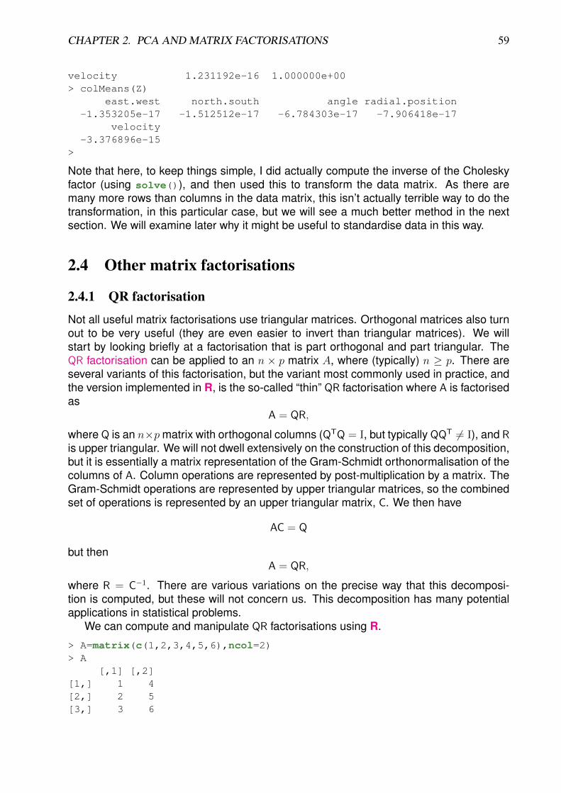
CHAPTER 2. PCA AND MATRIX FACTORISATIONS 59
velocity 1.231192e-16 1.000000e+00> colMeans(Z)
east.west north.south angle radial.position-1.353205e-17 -1.512512e-17 -6.784303e-17 -7.906418e-17
velocity-3.376896e-15
>
Note that here, to keep things simple, I did actually compute the inverse of the Choleskyfactor (using solve()), and then used this to transform the data matrix. As there aremany more rows than columns in the data matrix, this isn’t actually terrible way to do thetransformation, in this particular case, but we will see a much better method in the nextsection. We will examine later why it might be useful to standardise data in this way.
2.4 Other matrix factorisations
2.4.1 QR factorisation
Not all useful matrix factorisations use triangular matrices. Orthogonal matrices also turnout to be very useful (they are even easier to invert than triangular matrices). We willstart by looking briefly at a factorisation that is part orthogonal and part triangular. TheQR factorisation can be applied to an n × p matrix A, where (typically) n ≥ p. There areseveral variants of this factorisation, but the variant most commonly used in practice, andthe version implemented in R, is the so-called “thin” QR factorisation where A is factorisedas
A = QR,
where Q is an n×pmatrix with orthogonal columns (QTQ = I, but typically QQT 6= I), and Ris upper triangular. We will not dwell extensively on the construction of this decomposition,but it is essentially a matrix representation of the Gram-Schmidt orthonormalisation of thecolumns of A. Column operations are represented by post-multiplication by a matrix. TheGram-Schmidt operations are represented by upper triangular matrices, so the combinedset of operations is represented by an upper triangular matrix, C. We then have
AC = Q
but thenA = QR,
where R = C−1. There are various variations on the precise way that this decomposi-tion is computed, but these will not concern us. This decomposition has many potentialapplications in statistical problems.
We can compute and manipulate QR factorisations using R.
> A=matrix(c(1,2,3,4,5,6),ncol=2)> A
[,1] [,2][1,] 1 4[2,] 2 5[3,] 3 6
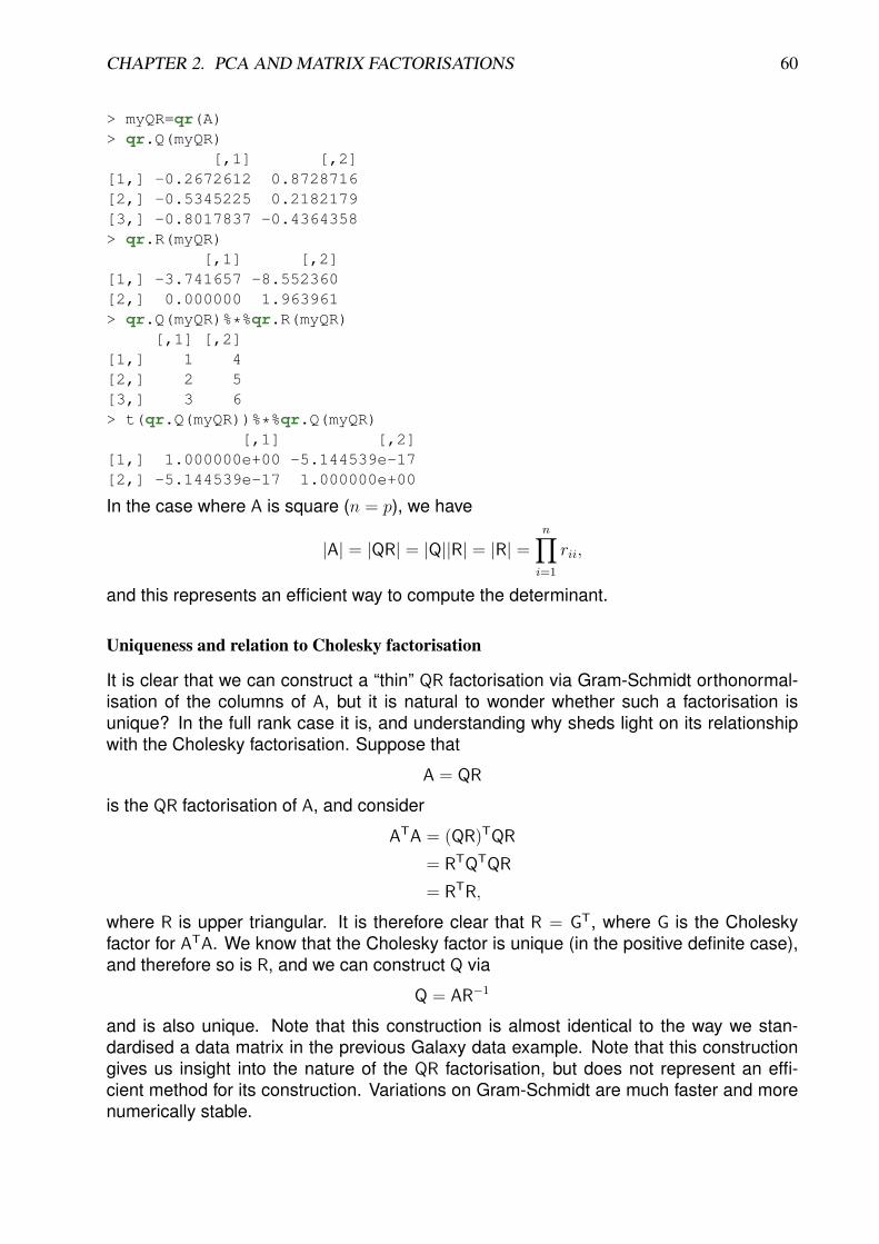
CHAPTER 2. PCA AND MATRIX FACTORISATIONS 60
> myQR=qr(A)> qr.Q(myQR)
[,1] [,2][1,] -0.2672612 0.8728716[2,] -0.5345225 0.2182179[3,] -0.8017837 -0.4364358> qr.R(myQR)
[,1] [,2][1,] -3.741657 -8.552360[2,] 0.000000 1.963961> qr.Q(myQR)%*%qr.R(myQR)
[,1] [,2][1,] 1 4[2,] 2 5[3,] 3 6> t(qr.Q(myQR))%*%qr.Q(myQR)
[,1] [,2][1,] 1.000000e+00 -5.144539e-17[2,] -5.144539e-17 1.000000e+00
In the case where A is square (n = p), we have
|A| = |QR| = |Q||R| = |R| =n∏i=1
rii,
and this represents an efficient way to compute the determinant.
Uniqueness and relation to Cholesky factorisation
It is clear that we can construct a “thin” QR factorisation via Gram-Schmidt orthonormal-isation of the columns of A, but it is natural to wonder whether such a factorisation isunique? In the full rank case it is, and understanding why sheds light on its relationshipwith the Cholesky factorisation. Suppose that
A = QR
is the QR factorisation of A, and consider
ATA = (QR)TQR
= RTQTQR
= RTR,
where R is upper triangular. It is therefore clear that R = GT, where G is the Choleskyfactor for ATA. We know that the Cholesky factor is unique (in the positive definite case),and therefore so is R, and we can construct Q via
Q = AR−1
and is also unique. Note that this construction is almost identical to the way we stan-dardised a data matrix in the previous Galaxy data example. Note that this constructiongives us insight into the nature of the QR factorisation, but does not represent an effi-cient method for its construction. Variations on Gram-Schmidt are much faster and morenumerically stable.
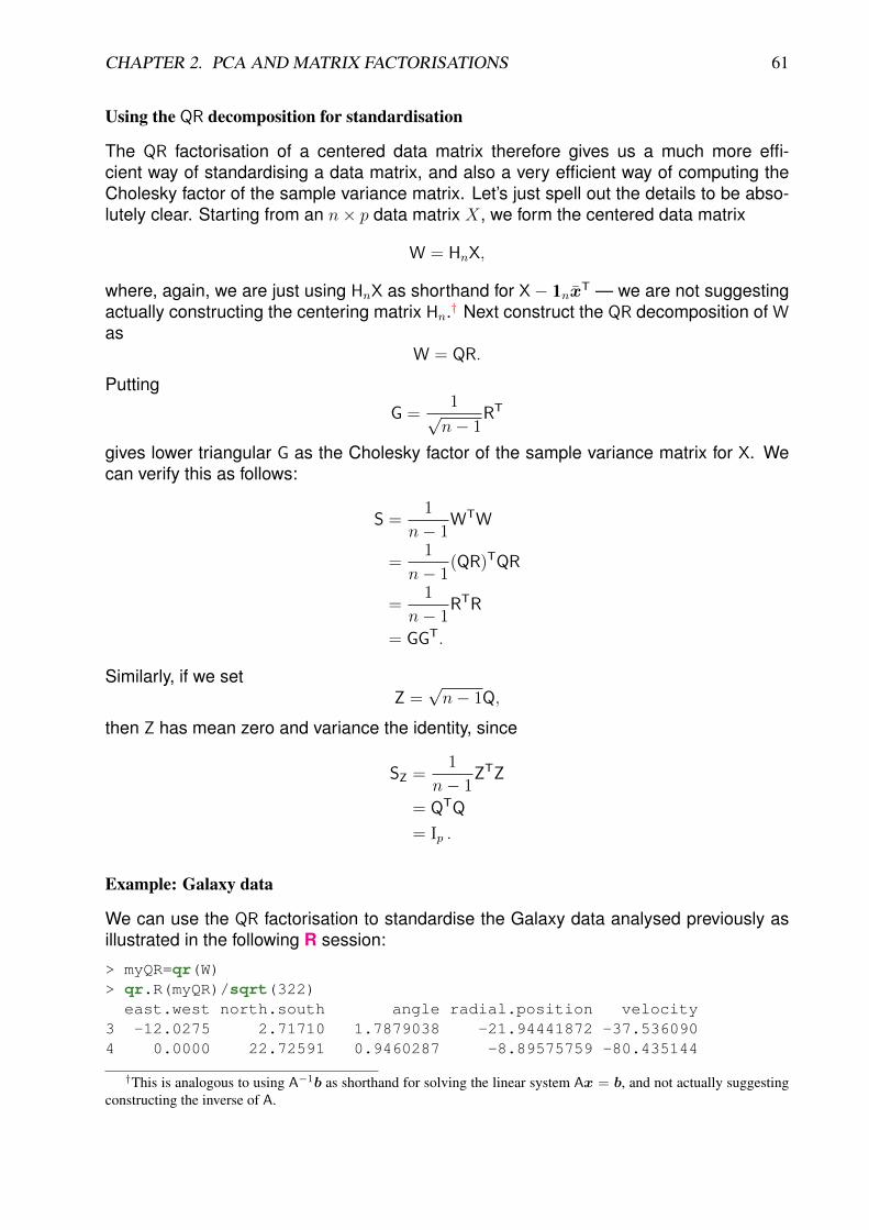
CHAPTER 2. PCA AND MATRIX FACTORISATIONS 61
Using the QR decomposition for standardisation
The QR factorisation of a centered data matrix therefore gives us a much more effi-cient way of standardising a data matrix, and also a very efficient way of computing theCholesky factor of the sample variance matrix. Let’s just spell out the details to be abso-lutely clear. Starting from an n× p data matrix X, we form the centered data matrix
W = HnX,
where, again, we are just using HnX as shorthand for X− 11nxT — we are not suggesting
actually constructing the centering matrix Hn.† Next construct the QR decomposition of Was
W = QR.
Putting
G =1√n− 1
RT
gives lower triangular G as the Cholesky factor of the sample variance matrix for X. Wecan verify this as follows:
S =1
n− 1WTW
=1
n− 1(QR)TQR
=1
n− 1RTR
= GGT.
Similarly, if we setZ =√n− 1Q,
then Z has mean zero and variance the identity, since
SZ =1
n− 1ZTZ
= QTQ
= Ip .
Example: Galaxy data
We can use the QR factorisation to standardise the Galaxy data analysed previously asillustrated in the following R session:
> myQR=qr(W)> qr.R(myQR)/sqrt(322)
east.west north.south angle radial.position velocity3 -12.0275 2.71710 1.7879038 -21.94441872 -37.5360904 0.0000 22.72591 0.9460287 -8.89575759 -80.435144
†This is analogous to using A−1b as shorthand for solving the linear system Ax = b, and not actually suggestingconstructing the inverse of A.
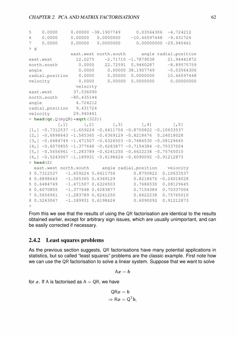
CHAPTER 2. PCA AND MATRIX FACTORISATIONS 62
5 0.0000 0.00000 -38.1907749 0.03564306 -4.7242126 0.0000 0.00000 0.0000000 -10.46597448 -9.4317247 0.0000 0.00000 0.0000000 0.00000000 -29.940461> g
east.west north.south angle radial.positioneast.west 12.0275 -2.71710 -1.7879038 21.94441872north.south 0.0000 22.72591 0.9460287 -8.89575759angle 0.0000 0.00000 38.1907749 -0.03564306radial.position 0.0000 0.00000 0.0000000 10.46597448velocity 0.0000 0.00000 0.0000000 0.00000000
velocityeast.west 37.536090north.south -80.435144angle 4.724212radial.position 9.431724velocity 29.940461> head(qr.Q(myQR)*sqrt(322))
[,1] [,2] [,3] [,4] [,5][1,] -0.7312537 -1.659224 -0.6411756 -0.8750822 -0.10633537[2,] -0.6898643 -1.565365 -0.6369129 -0.8218676 0.24018028[3,] -0.6484749 -1.471507 -0.6326503 -0.7686530 -0.08129645[4,] -0.6070855 -1.377648 -0.6283877 -0.7154384 -0.70337004[5,] -0.5656961 -1.283789 -0.6241250 -0.6622238 -0.75765010[6,] -0.5243067 -1.189931 -0.6198624 -0.6090092 -0.91212873> head(Z)east.west north.south angle radial.position velocity
3 0.7312537 -1.659224 0.6411756 0.8750822 0.106335374 0.6898643 -1.565365 0.6369129 0.8218676 -0.240180285 0.6484749 -1.471507 0.6326503 0.7686530 0.081296456 0.6070855 -1.377648 0.6283877 0.7154384 0.703370047 0.5656961 -1.283789 0.6241250 0.6622238 0.757650108 0.5243067 -1.189931 0.6198624 0.6090092 0.91212873>
From this we see that the results of using the QR factorisation are identical to the resultsobtained earlier, except for arbitrary sign issues, which are usually unimportant, and canbe easily corrected if necessary.
2.4.2 Least squares problems
As the previous section suggests, QR factorisations have many potential applications instatistics, but so called “least squares” problems are the classic example. First note howwe can use the QR factorisation to solve a linear system. Suppose that we want to solve
Ax = b
for x. If A is factorised as A = QR, we have
QRx = b
⇒ Rx = QTb,
CHAPTER 2. PCA AND MATRIX FACTORISATIONS 63
since QTQ = I, and then we can solve for x using backward substitution.Now consider the classical multiple linear regression problem
y = Xβ + ε.
Given data y and X we want to find the β which minimises ‖ε‖22 = εTε. Differentiating withrespect to the vector β and equating to zero leads to the so-called “normal equations”
XTXβ = XTy.
The classical method for solving these equations was via a Cholesky decomposition forXTX and then backward and forward substitution. However, it turns out to be more efficientand numerically stable to use the QR factorisation of X, as
(QR)TQRβ = (QR)Ty
⇒ RTQTQRβ = RTQTy
⇒ RTRβ = RTQTy
⇒ β = (RTR)−1RTQTy
= R−1R−TRTQTy
⇒ β = R−1QTy.
That is, β is the solution ofRβ = QTy,
obtained by backward substitution. This is the method of solution used by R’s lm() func-tion.
2.4.3 Spectral decomposition
Construction for real symmetric matrices
Recall that v is an eigenvector of an n × n square matrix A, and λ is its correspondingeigenvalue if
Av = λv
Clearly (A− λ I)v = 0, so v is in the null-space of A− λ I, which means that this must besingular, and so eigenvalues can be identified as roots of the characteristic equation
|A− λ I | = 0.
Since this is a polynomial in λ of degree n, there are n (not necessarily distinct) eigenval-ues of A. In general, some of these eigenvalues will be complex, but not if A is symmetric.
Proposition 17 The eigenvalues of a real symmetric matrix A are real.
ProofSuppose that λ is a complex eigenvalue of A. In this case the corresponding eigen-
vector v is also complex. By definition we have Av = λv, and taking complex conjugateswe have
Av = λv
CHAPTER 2. PCA AND MATRIX FACTORISATIONS 64
so λ is also an eigenvalue with corresponding eigenvector v.‡ But then
vTAv = λv†v = λv†v
⇒ λ‖v‖2 = λ‖v‖2
⇒ λ = λ,
and so λ ∈ R. �
Since we can choose the magnitude of an eigenvector arbitrarily, we will assume that wealways choose eigenvectors to have norm 1. That is vTv = 1.
Proposition 18 The eigenvectors corresponding to distinct eigenvalues of a real sym-metric matrix A are orthogonal.
Proof
Suppose that (λ1,v1) and (λ2,v2) are both eigen-pairs of A.Then
v1TAv2 = λ2v1
Tv1 = λ1v1Tv2
⇒ (λ2 − λ2)v1 · v2 = 0,
so either λ1 = λ2 or v1 · v2 = 0.�
In fact, it turns out that repeated eigenvalues do not complicate the picture, since theeigen-space corresponding to repeated eigenvalues has the same dimension as the mul-tiplicity of the root, and hence orthogonal eigenvectors may also be constructed for therepeated eigenvalues. Hence we can order the eigenvalues in decreasing order as
Avi = λivi, i = 1, 2, . . . , n
and by stacking the eigenvectors as columns of an n × n orthogonal matrix V we canre-write the above equations as
AV = VD
where D = diag {λ1, λ2, . . . , λn}. This then leads to one of the most important results inlinear algebra.
Proposition 19 (Spectral decomposition) If A is a real symmetric n × n matrix, it canbe factorised in the form
A = VDVT
where V is an orthogonal matrix whose columns are the eigenvectors of A and D =diag {λ1, λ2, . . . , λn}, where the λi are the ordered eigenvalues of A corresponding to theeigenvectors in the columns of V.
We will often be interested in symmetric matrices which are positive semi-definite. Thesematrices clearly have non-negative eigenvalues, and similarly, strictly positive definite ma-trices have strictly positive eigenvalues.‡Note that here we are using a bar (¯) to denote complex conjugation, rather than a sample mean. This proof is the
only place in the whole course where complex numbers occur, and hence the only place where a bar does not representa sample mean. Here we also use a dagger for conjugate transpose. That is, v† = vT.
CHAPTER 2. PCA AND MATRIX FACTORISATIONS 65
Symmetric square root
The spectral decomposition can be used to create a symmetric square root matrix, sinceif
A = VDVT
thenG = VD1/2VT
satisfies GT = G and GG = A, and hence also GGT = A. This symmetric square rootis a “true” square root matrix, unlike the Cholesky triangle. It is also well defined forsingular positive semi-definite matrices, where use of the Cholesky decomposition can beproblematic. In the positive definite case, we can also directly construct its inverse as
G−1 = VD−1/2VT,
which can be very useful in several contexts. The symmetry of this square root matrix isalso desirable in some applications. However, the Cholesky factorisation is much fasterthan an eigen-solver, so in the many applications where the cheaper Cholesky factor willbe adequate, it is usually to be preferred.
Example: toy problem
Construct the spectral decomposition of the matrix
A =
(9 77 9
),
and use it to construct a symmetric square root, G, of A. Verify that G2 = A.
We first find roots of the characteristic equation via
|A− λ I | =∣∣∣∣ 9− λ 7
7 9− λ
∣∣∣∣= (9− λ)2 − 49
= (λ− 2)(λ− 16).
So the ordered eigenvalues are λ1 = 16, λ2 = 2. Now
A− λ1 I =
(−7 7
7 −7
),
and sov1 =
1√2
(1
1
).

CHAPTER 2. PCA AND MATRIX FACTORISATIONS 66
Similarly,
A− λ2 I =
(7 7
7 7
),
sov2 =
1√2
(1
−1
).
Consequently, our spectral decomposition is A = VDVT, where
V =1√2
(1 1
1 −1
), D =
(16 0
0 2
).
Now we have the spectral decomposition, it is straightforwardto construct the symmetric square root as
G = VD1/2VT
=1
2
(1 1
1 −1
)(4 0
0√
2
)(1 1
1 −1
)=
1
2
(1 1
1 −1
)(4 4√2 −√
2
)=
1
2
(4 +√
2 4−√
2
4−√
2 4 +√
2
).
Our proposed square root is clearly symmetric, and we canverify that it is indeed a square root with
G2 =1
4
(4 +√
2 4−√
2
4−√
2 4 +√
2
)(4 +√
2 4−√
2
4−√
2 4 +√
2
)=
1
4
(36 28
28 36
)= A.
2.4.4 Mahalanobis transformation and distance
Mahalanobis transformation
The Mahalanobis transformation is just a standardisation transformation using the (in-verse) symmetric square root of the variance matrix. So if X is a random vector withmean µ and variance matrix Σ, the Mahalanobis transformation is
Z = Σ−1/2(X − µ),

CHAPTER 2. PCA AND MATRIX FACTORISATIONS 67
where Σ−1/2 is the inverse of the symmetric square root of Σ. Z will have mean 0 andvariance I.
Similarly, if X is an n× p data matrix, the Mahalanobis transform is
Z = HnXS−1/2,
though again, it must be emphasised that this is a mathematical description of the trans-formation, and not a recipe for how to construct it numerically. Z will have sample meanzero and sample variance Ip.
Example: Galaxy data
We will look now at how to compute the spectral decomposition of the galaxy data setusing R, and how to use it to construct a symmetric square root, and its inverse.
> v=var(galaxy)> v
east.west north.south angle radial.positioneast.west 144.66088 -32.67993 -21.50402 263.93661north.south -32.67993 523.84971 26.35728 -261.78938angle -21.50402 26.35728 1462.62686 -49.01139radial.position 263.93661 -261.78938 -49.01139 670.22991velocity 451.46551 -1929.95131 37.21646 1637.78301
velocityeast.west 451.46551north.south -1929.95131angle 37.21646radial.position 1637.78301velocity 8886.47724> e=eigen(v,symmetric=TRUE)> e$values[1] 9642.07343 1466.48964 487.88910 68.87222 22.52020
$vectors[,1] [,2] [,3] [,4] [,5]
[1,] 0.051396600 0.02254908 0.45279536 0.1122205 0.88274167[2,] -0.208493672 -0.01789604 0.31495251 0.8879502 -0.26183862[3,] 0.002463535 -0.99826125 0.04727651 -0.0346832 0.00551559[4,] 0.182722226 0.05000384 0.82508240 -0.3634307 -0.38893366[5,] 0.959424462 -0.01205694 -0.11307185 0.2562542 -0.03013096
> e$vectors%*%t(e$vectors)[,1] [,2] [,3] [,4]
[1,] 1.000000e+00 -7.224852e-17 -4.978182e-17 1.115915e-16[2,] -7.224852e-17 1.000000e+00 1.760090e-16 -8.700722e-18[3,] -4.978182e-17 1.760090e-16 1.000000e+00 2.170533e-16[4,] 1.115915e-16 -8.700722e-18 2.170533e-16 1.000000e+00[5,] 2.232271e-17 -1.676939e-16 -1.400287e-16 8.567399e-17
[,5][1,] 2.232271e-17
CHAPTER 2. PCA AND MATRIX FACTORISATIONS 68
[2,] -1.676939e-16[3,] -1.400287e-16[4,] 8.567399e-17[5,] 1.000000e+00> e$vectors%*%diag(e$values)%*%t(e$vectors)
[,1] [,2] [,3] [,4] [,5][1,] 144.66088 -32.67993 -21.50402 263.93661 451.46551[2,] -32.67993 523.84971 26.35728 -261.78938 -1929.95131[3,] -21.50402 26.35728 1462.62686 -49.01139 37.21646[4,] 263.93661 -261.78938 -49.01139 670.22991 1637.78301[5,] 451.46551 -1929.95131 37.21646 1637.78301 8886.47724> G=e$vectors%*%diag(sqrt(e$values))%*%t(e$vectors)> G
[,1] [,2] [,3] [,4] [,5][1,] 8.6098647 1.8123819 -0.3859399 7.2496158 3.8132008[2,] 1.8123819 13.3404531 0.7001528 -0.2300872 -18.4947058[3,] -0.3859399 0.7001528 38.2218104 -0.9113324 0.5003811[4,] 7.2496158 -0.2300872 -0.9113324 20.2249833 14.4131733[5,] 3.8132008 -18.4947058 0.5003811 14.4131733 91.2244082> G%*%G
[,1] [,2] [,3] [,4] [,5][1,] 144.66088 -32.67993 -21.50402 263.93661 451.46551[2,] -32.67993 523.84971 26.35728 -261.78938 -1929.95131[3,] -21.50402 26.35728 1462.62686 -49.01139 37.21646[4,] 263.93661 -261.78938 -49.01139 670.22991 1637.78301[5,] 451.46551 -1929.95131 37.21646 1637.78301 8886.47724> Ginv=e$vectors%*%diag(1/sqrt(e$values))%*%t(e$vectors)> G%*%Ginv
[,1] [,2] [,3] [,4][1,] 1.000000e+00 -2.478825e-16 -2.061869e-17 1.212003e-16[2,] -2.428952e-16 1.000000e+00 3.009745e-16 1.170261e-16[3,] -1.111113e-15 8.248890e-16 1.000000e+00 1.020284e-15[4,] 6.617055e-16 -3.846478e-16 2.830987e-16 1.000000e+00[5,] 8.075138e-16 -1.285430e-15 -4.671759e-16 -4.477755e-17
[,5][1,] 1.171616e-17[2,] -2.679606e-16[3,] -1.481901e-16[4,] 8.386304e-17[5,] 1.000000e+00
Now we have Ginv we can use it to construct the Mahalanobis transform of the data
> W=sweep(galaxy,2,colMeans(galaxy))> Z=as.matrix(W)%*%Ginv> colMeans(Z)[1] 4.419302e-16 -2.600506e-15 2.784151e-17 1.075502e-15[5] -1.821798e-15> var(Z)
[,1] [,2] [,3] [,4][1,] 1.000000e+00 6.811770e-16 -8.034862e-16 1.586732e-15
CHAPTER 2. PCA AND MATRIX FACTORISATIONS 69
[2,] 6.811770e-16 1.000000e+00 1.309490e-15 5.266862e-15[3,] -8.034862e-16 1.309490e-15 1.000000e+00 4.550018e-16[4,] 1.586732e-15 5.266862e-15 4.550018e-16 1.000000e+00[5,] -3.265377e-16 -2.529045e-15 -2.198962e-16 1.568981e-15
[,5][1,] -3.265377e-16[2,] -2.529045e-15[3,] -2.198962e-16[4,] 1.568981e-15[5,] 1.000000e+00
Mahalanobis distance
Given an observation x of a random vector X with E(X) = µ and Var(X) = Σ, it isnatural to wonder how “unusual” it is, in some appropriate sense. We cannot give a veryformal solution to this problem until we develop some multivariate distribution theory, buteven now we can give an intuitive explanation of the most commonly used summary. Insome sense we want to know how “far” the observation is from the mean, but in generalsome components are more variable than others, so it doesn’t make sense to look at“distance” on the scale of the original variables. However, it does make perfect sense fora standardised observation, z. So the Mahalanobis distance of x from µ is just
‖z‖ =√zTz
=√
[Σ−1/2(x− µ)] TΣ−1/2(x− µ)
=√
(x− µ)TΣ−1(x− µ).
Computationally, the efficient way to compute this distance measure is as√zTz where
z = Σ−1/2(x− µ).
Note that it is not necessary to use a symmetric square root for this computation. Stan-dardisation using the Cholesky factor leads to exactly the same distance, and is muchcheaper to compute and then solve than using a symmetric square root. Confirmation ofthis fact is left as an exercise.
It is also worth noting that if the variance is defined empirically, as the sample variancematrix S of a data matrix X, then the Mahalanobis distance can be calculated yet morestably and efficiently using the QR factorisation of X.
Computing the Mahalanobis distance for each observation in a data set is the mostcommonly used technique for identifying outlying observations in multivariate data.
Example: Galaxy data
Continuing our previous example, we have already constructed a standardised data matrixZ using a Mahalanobis transformation. We can use it to construct a Mahalanobis distancefor each observation as follows.
d=sqrt(apply(Z*Z,1,sum))
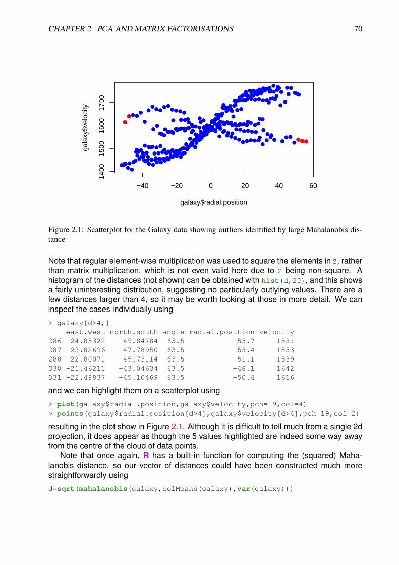
CHAPTER 2. PCA AND MATRIX FACTORISATIONS 70
●●●●●●●●
●
●●●
●●●
●●
●●
●●
●●
●●●
●●
●●●●●●
●
●
●
●●
●●●●●●●
●
●●●●
●●
●●●●
●●●
●
●●●●●●●●●●
●●
●
●●
●
●●●
●●
●●●●●●●●●●●●
●●
●●●●●
●
●●●●
●●●●●
●
●●●
●
●●
●●
●●●
●
●●●●
●●●●●●
●●●
●●●●
●●●
●
●●●●●●●●●
●●
●●●
●
●
●●
●●
●
●
●●
●
●
●●
●
●●●●●
●
●●
●
●●
●
●●
●●
●●●●
●●
●●●●●●●
●
●●●
●●●●
●●●●
●●
●●●●●●
●●●●●
●
●●●
●●
●●
●
●●●●●●
●●●
●
●
●●●●
●●
●●●
●●●●●●●●
●●●●●
●●
●●●●●●
●●
●
●
●●●
●●●●●●●
●●
●●●
●●
●●
●●
●●●
●●●●●●●●●●●
●●●
●●●
−40 −20 0 20 40 60
1400
1500
1600
1700
galaxy$radial.position
gala
xy$v
eloc
ity
●●●
●
●
Figure 2.1: Scatterplot for the Galaxy data showing outliers identified by large Mahalanobis dis-tance
Note that regular element-wise multiplication was used to square the elements in Z, ratherthan matrix multiplication, which is not even valid here due to Z being non-square. Ahistogram of the distances (not shown) can be obtained with hist(d,20), and this showsa fairly uninteresting distribution, suggesting no particularly outlying values. There are afew distances larger than 4, so it may be worth looking at those in more detail. We caninspect the cases individually using
> galaxy[d>4,]east.west north.south angle radial.position velocity
286 24.85322 49.84784 63.5 55.7 1531287 23.82696 47.78950 63.5 53.4 1533288 22.80071 45.73114 63.5 51.1 1539330 -21.46211 -43.04634 63.5 -48.1 1642331 -22.48837 -45.10469 63.5 -50.4 1616
and we can highlight them on a scatterplot using
> plot(galaxy$radial.position,galaxy$velocity,pch=19,col=4)> points(galaxy$radial.position[d>4],galaxy$velocity[d>4],pch=19,col=2)
resulting in the plot show in Figure 2.1. Although it is difficult to tell much from a single 2dprojection, it does appear as though the 5 values highlighted are indeed some way awayfrom the centre of the cloud of data points.
Note that once again, R has a built-in function for computing the (squared) Maha-lanobis distance, so our vector of distances could have been constructed much morestraightforwardly using
d=sqrt(mahalanobis(galaxy,colMeans(galaxy),var(galaxy)))
CHAPTER 2. PCA AND MATRIX FACTORISATIONS 71
2.4.5 The singular value decomposition (SVD)
The final matrix factorisation we will examine here, the singular value decomposition, canbe applied to arbitrary n × p matrices (we typically consider the case n ≥ p), and isclosely related to both the QR factorisation and the spectral decomposition. As for the QRfactorisation, there are a few variants, and we concentrate here on a variant known as the“thin” SVD, as it is the most commonly used in practice.
Proposition 20 The n× p matrix A can be factorised as
A = UDVT,
where U is an n × p matrix with orthonormal columns (UTU = Ip), D is a p × p diagonalmatrix with non-negative entries, and V is a p× p orthogonal matrix. The diagonal entriesof D are known as the singular values of A. The columns of U are known as the leftsingular vectors, and the columns of V are known as the right singular vectors.
ProofConsider the spectral decomposition of ATA, which is clearly p × p, real, symmetric,
and positive semi-definite. We can therefore write the spectral decomposition in the form
ATA = VD2VT,
as the eigenvalues are non-negative. By construction, V is an orthogonal matrix. We nowput
U = AVD−1,
to get the SVD A = UDVT, and we verify that the columns of U are orthogonal as
UTU = (AVD−1)T(AVD−1)
= D−1VTATAVD−1
= D−1VTVD2VTVD−1
= D−1D2D−1
= Ip .
�
It must be emphasised that this is a mathematical construction to demonstrate the exis-tence of the factorisation, and its relationship to the spectral decomposition, but this is nothow the factorisation is constructed in practice (and in any case, there are issues with thisconstruction when D is singular). There are very efficient methods which can be used forthis, often starting from a QR factorisation of A. Typically ATA is not constructed at all, asthis is a numerically unstable computation.
The SVD and spectral decomposition
From our construction it is clear that the columns of V are the eigenvectors of ATA, so theleft singular vectors are eigenvectors of ATA. Similarly, the n × n matrix AAT = UD2UT.Now U is n× p, but post-multiplying by U gives
(AAT)U = UD2,
CHAPTER 2. PCA AND MATRIX FACTORISATIONS 72
and so the columns of U are eigenvectors of AAT corresponding to the p eigenvalues inD2, which includes all of the non-zero eigenvalues of AAT. So the right singular vectorsare (the important) eigenvectors of AAT.
It should be clear that if the SVD is applied directly to a real symmetric positive semi-definite matrix, that the spectral decomposition is obtained. Numerically, however, thealgorithms used to calculate the SVD are quite different to those typically used for eigen-solvers. The SVD will typically be slightly slower than a symmetric eigen-solver but fasterthan an asymmetric eigen-solver. The SVD may be more numerically stable if the inputmatrix is close to singular, and is therefore very commonly used in practice.
SVD for least squares
The SVD provides an alternative approach to solving the normal equations
XTXβ = XTy
for β.
Let X = UDVT be the SVD of X, and then
XTXβ = XTy
⇒ (UDVT)T(UDVT)β = (UDVT)Ty
⇒ VDUTUDVTβ = VDUTy
⇒ VD2VTβ = VDUTy
⇒ DVTβ = UTy
⇒ β = VD−1UTy.
This turns out to be a numerically stable way of solving (full rank) least squares prob-lems, but since the SVD is slower than the QR factorisation, the previously described QRmethod is usually to be preferred.
Symmetrising a Cholesky factor
Note that a Cholesky factor may be converted into the symmetric square root via the SVD.Suppose that the Cholesky decomposition of A is
A = LLT.
Then suppose that we form the SVD of L as
L = UDVT,
so thatA = (UDVT)(UDVT)T = UD2UT.
If we putG = UDUT,
it is clear that G is symmetric, and that G2 = A, and hence is the symmetric square root.
CHAPTER 2. PCA AND MATRIX FACTORISATIONS 73
Example: Galaxy data
We can form the SVD of the variance matrix for the galaxy data set using
> svd(var(galaxy))$d[1] 9642.07343 1466.48964 487.88910 68.87222 22.52020
$u[,1] [,2] [,3] [,4] [,5]
[1,] -0.051396600 -0.02254908 -0.45279536 -0.1122205 0.88274167[2,] 0.208493672 0.01789604 -0.31495251 -0.8879502 -0.26183862[3,] -0.002463535 0.99826125 -0.04727651 0.0346832 0.00551559[4,] -0.182722226 -0.05000384 -0.82508240 0.3634307 -0.38893366[5,] -0.959424462 0.01205694 0.11307185 -0.2562542 -0.03013096
$v[,1] [,2] [,3] [,4] [,5]
[1,] -0.051396600 -0.02254908 -0.45279536 -0.1122205 0.88274167[2,] 0.208493672 0.01789604 -0.31495251 -0.8879502 -0.26183862[3,] -0.002463535 0.99826125 -0.04727651 0.0346832 0.00551559[4,] -0.182722226 -0.05000384 -0.82508240 0.3634307 -0.38893366[5,] -0.959424462 0.01205694 0.11307185 -0.2562542 -0.03013096
We see that it is exactly the same as the spectral decomposition obtained earlier, modulosome sign changes on some of the columns, which are arbitrary.
2.5 Principal components analysis (PCA)
2.5.1 Derivation from the spectral decomposition
Principal components analysis, or PCA as it is more commonly known, is a techniquefor finding interesting low dimensional projections of a multivariate random variable or,more commonly, data matrix. It is very closely related to the spectral decompositionand SVD. We will begin by understanding principal components in relation to the eigen-decomposition of a variance matrix. To keep things as simple as possible, we begin byconsidering a p-dimensional random vector X with E(X) = µ and Var(X) = Σ. Writethe spectral decomposition of Σ as
Σ = VDVT.
Now consider a linear combination αTX, or one-dimensional projection of X, a scalarrandom quantity for given fixed p-dimensional α. We know that the variance of this linearcombination is αTΣα. Let us now consider the linear combination represented by theeigenvectors in the columns of V. The ith eigenvector, vi, corresponding to the eigenvalueλi, has variance
viTΣvi = λivi
Tvi = λi.
So the eigenvalues are the variances of the linear combinations represented by the cor-responding eigenvectors. Similarly, if we consider the correlation between the random
CHAPTER 2. PCA AND MATRIX FACTORISATIONS 74
quantities represented by two distinct eigenvectors, vi, vj, we have
Cov(vi
TX,vjTX)
= viT Cov(X,X)vj = vi
TΣvj = λjviTvj = 0.
So the eigenvectors form a basis for the space of linear combinations of X, and repre-sent a collection of uncorrelated random quantities whose variances are given by theirrespective eigenvalues.
Formally we characterise principal components as linear combinations of variablesthat explain the greatest variation in the random quantity or data set. However, we needto place a constraint on the linear combination for this to be well defined. For example,if αTX is a linear combination with variance σ2, then it is clear that kαTX has variancek2σ2, so we can make the variance of a linear combination as large as we wish simply bymultiplying it by a large enough scalar. However, we are really interested in the directionwith largest variation, and so we impose the constraint ‖α‖ = 1, or αTα = 1. To maximisesubject to a non-linear constraint we use a Lagrange multiplier, and begin by optimising
f = αTΣα− λ(αTα− 1)
= αT(Σ− λ I)α+ λ.
Now, recalling that for a symmetric matrix A, we have
∇xTAx =∂
∂xxTAx = 2Ax,
we can differentiate and equate to zero to get
∂f
∂x= 2(Σ− λ I)α = 0.
In other words,|Σ− λ I | = 0,
and λ is an eigenvalue of Σ, and α is the (normalised) eigenvector corresponding to λ.Since we typically construct the spectral decomposition with eigenvalues in decreasingorder, we pick the solution with largest variance as
λ = λ1, α = v1.
So the first eigenvector of the spectral decomposition represents the linear combinationof variables with the largest variance, and its variance is given by its corresponding eigen-value. This is the first principal component.
The second principal component is defined to be the linear combination uncorrelatedwith the first principal component which has the greatest variance. But since we haveseen that the linear combinations corresponding to the eigenvectors are uncorrelated, itfollows that the set of linear combinations corresponding to quantities uncorrelated withthe first principal component is spanned by the 2nd to pth eigenvectors, and hence themaximum variance will be obtained at λ2, corresponding to the 2nd eigenvector, v2. Thethird principal component is the linear combination with greatest variance uncorrelatedwith the first two principal components, and so on. So we see that there is a direct corre-spondence between the spectral decomposition of the variance matrix and the principalcomponents of the random vector.
CHAPTER 2. PCA AND MATRIX FACTORISATIONS 75
We can associate each principal component with a random quantity, Yi = viTX, i =
1, 2, . . . , p, and use these to construct a new random vector
Y = VTX,
the vector of principal components. The variance matrix of Y is clearly given by
Var(Y ) = Var(VTX
)= VT Var(X) V
= VTVDVTV
= D.
So the components of Y are uncorrelated, and each has the correct variance, as required.
2.5.2 Total variation and variance explained
We know that the variance matrix is a very rich summary of the variability of a random vec-tor, X. However, sometimes it is useful to have a single scalar summary which capturessome aspect of the overall variability of the random vector. There are obviously manyways that this could be done, and none will be perfect, but a commonly used summary ofvariation is the sum of the variances of the individual variables,
t(X) =
p∑i=1
Var(Xi) = Tr (Var(X)) ,
often known as the total variation of the random vector. The total variation has the de-sirable property that it is preserved by orthogonal rotation. In particular, if we considertransforming X to its principal components via
Y = VTX
we have
t(X) = Tr (Var(X))
= Tr(VDVT
)= Tr
(DVTV
)= Tr (D)
= t(Y ),
using the fact that Tr (AB) = Tr (BA) for square matrices.One motivation for undertaking principal components analysis is to try and find low-
dimensional projections of the original variables which contain most of the information inthe original higher-dimensional vectors. One way of characterising the information is byits variation. Since the principal components are ordered with most variable first, it makessense to consider the first q principal components (q ≤ p). The total variation of the first qprincipal components is clearly
∑qi=1 λi. The proportion of variance explained is thereforeq∑i=1
λi
p∑i=1
λi
=1
Tr (D)
q∑i=1
λi,
CHAPTER 2. PCA AND MATRIX FACTORISATIONS 76
with the proportion increasing to 1 by q = p. Therefore an obvious strategy for dimensionreduction is to work with the first q principal components, where q is the smallest numbersuch that the proportion of variance explained exceeds a given pre-specified threshold.The actual threshold will be problem dependent — there are no hard-and-fast rules, asprincipal components are primarily an exploratory tool.
2.5.3 Principal components from a sample variance matrix
To keep the notation simple we have introduced the idea of principal components for arandom vector. However, in practice principal components analysis is mainly used in theanalysis of multivariate data. So now suppose that we have an n× p data matrix, X, andwish to use principal components analysis to find interesting low-dimensional projections.Let us suppose that we have the sample variance matrix
S =1
n− 1XTHnX
and form its spectral decomposition as
S = VDVT.
Then all of the properties we described for random variables easily follow. For example,the eigenvectors in the columns of V correspond to linear combinations of the variableswhose sample variance is the corresponding eigenvalue, and distinct eigenvectors corre-spond to linear combinations of variables whose sample covariance is zero. So we candefine the first principal component of X to be the linear combination of variables whosesample variance is largest (subject to the unit norm constraint), and it trivially follows thatthis corresponds to the first eigenvector, v1, and its sample variance is λ1. Similarly thesecond principal component corresponds to v2, with sample variance λ2, and so on.
We can obviously transform observations to their principal component representationusing
y = VTx
and so we can transform X to Y, the data rotated to the principal component axes, using
Y = XV.
However, in practice the data are usually centered before rotating, so in practice the trans-formation
Y = HnXV
is used.§ In the context of principal components analysis, the matrix of eigenvectors, V,is often known as the loadings matrix, and the transformed observations in Y are oftenknown as component scores.§The usual caveat about not actually using the centering matrix to center the data applies.

CHAPTER 2. PCA AND MATRIX FACTORISATIONS 77
●●●●●●●●●●●●●● ●●●● ●●●● ●●●●●●●●●●● ●● ●●
●●●●●●●● ● ●●●●●● ● ●●●●●● ●●
●●●●●●●●●●● ● ●●●●●●●●●●●●●●●● ●●●●●●●
●● ●●●● ● ●●●●●●●●●● ●●● ●●●●●●●●●●●●●●●●●● ● ●●●●●●
●● ●● ●●●●●●●● ● ● ●●● ● ●● ● ● ●●● ●●●
●● ●●● ●●●●●●●●● ●●●●● ●●●●●●●●●●●●●●● ●●●●
●●●● ●●●● ●●● ●●●●● ●●●● ●● ● ●● ● ●●● ● ●●●● ●●●● ●●● ●●●●●
●●● ●●●●●●●●●●●●●●● ● ●●●●●●●●
●● ●● ●●●●●●●●●●●●●●●●●●●●●●●●●●●●●●●●● ●●●●● ●
−200 −100 0 100 200
−40
020
60
Y[, 1]
Y[,
2]
Figure 2.2: Scatterplot for the Galaxy data showing the second principal component plotted againstthe first
Example: Galaxy data
We will begin by constructing a PCA “by hand” using the spectral decomposition of thesample variance matrix. We will use the objects v (the sample variance matrix), W (thecentered data matrix) and e (the spectral decomposition of v) from the previous example.We can examine the variance explained by the principal components using
> cumsum(e$values)/sum(e$values)[1] 0.8249659 0.9504373 0.9921806 0.9980732 1.0000000
So we see that the first principal component already explains over 80% of the total varia-tion, and the first two together explain over 95% of the variation. We should therefore get avery adequate representation of the data by projection into the first two components, andessentially all of the variation is explained by the first 3 components. We can constructthe principal component scores with
Y=as.matrix(W)%*%e$vectors
We can plot the second principal component against the first using
plot(Y[,1],Y[,2],pch=19,col=galaxy$angle)
giving the plot shown in Figure 2.2.As can be verified by inspecting the factor loading matrix, the first principal component
is dominated by velocity and the second is dominated by angle. We have rotatedthe data to find a 2d projection where the observations are as “spread out” as possible.We can also plot the third principal component against the first (not shown) in order toget information “orthogonal” to the angle dominated principal component. In fact, if thergl package is installed, we can produce an interactive 3d plot of the first 3 principalcomponents as
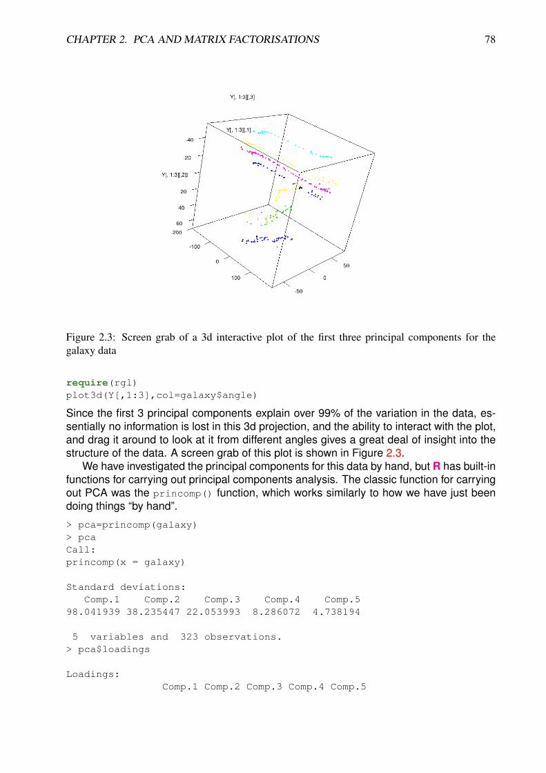
CHAPTER 2. PCA AND MATRIX FACTORISATIONS 78
Figure 2.3: Screen grab of a 3d interactive plot of the first three principal components for thegalaxy data
require(rgl)plot3d(Y[,1:3],col=galaxy$angle)
Since the first 3 principal components explain over 99% of the variation in the data, es-sentially no information is lost in this 3d projection, and the ability to interact with the plot,and drag it around to look at it from different angles gives a great deal of insight into thestructure of the data. A screen grab of this plot is shown in Figure 2.3.
We have investigated the principal components for this data by hand, but R has built-infunctions for carrying out principal components analysis. The classic function for carryingout PCA was the princomp() function, which works similarly to how we have just beendoing things “by hand”.
> pca=princomp(galaxy)> pcaCall:princomp(x = galaxy)
Standard deviations:Comp.1 Comp.2 Comp.3 Comp.4 Comp.5
98.041939 38.235447 22.053993 8.286072 4.738194
5 variables and 323 observations.> pca$loadings
Loadings:Comp.1 Comp.2 Comp.3 Comp.4 Comp.5

CHAPTER 2. PCA AND MATRIX FACTORISATIONS 79
east.west 0.453 0.112 0.883north.south -0.208 0.315 0.888 -0.262angle -0.998radial.position 0.183 0.825 -0.363 -0.389velocity 0.959 -0.113 0.256
Comp.1 Comp.2 Comp.3 Comp.4 Comp.5SS loadings 1.0 1.0 1.0 1.0 1.0Proportion Var 0.2 0.2 0.2 0.2 0.2Cumulative Var 0.2 0.4 0.6 0.8 1.0> dim(pca$scores)[1] 323 5> plot(pca$scores[,1],pca$scores[,2],pch=19,col=galaxy$angle)
The final command produces a plot very similar to Figure 2.2. Also note that summary(pca) will print some additional information and that plot(pca) will produce a barplotindicating the variances of the principal components.
2.5.4 Construction from the SVD
Although the spectral decomposition of the variance matrix is a conceptually elegant wayto understand principal components, it turns out that constructing them this way from asample variance matrix is inefficient and numerically unstable. Starting from a data matrixX, we first compute the centred data
W = HnX.
Then the sample variance matrix is given by
S =1
n− 1WTW.
If we were to follow the usual approach, we could go on to form the spectral decompositionof S and construct principal components as before. However, it turns out that we can avoidthe computation of S completely using a SVD of the centered data W. Putting
W = UDVT
we see that
S =1
n− 1WTW
=1
n− 1VDUTUDVT
=1
n− 1VD2VT
= VΛVT,
whereΛ =
1
n− 1D2.
CHAPTER 2. PCA AND MATRIX FACTORISATIONS 80
We have therefore constructed the spectral decomposition of S directly from the SVDof W, and the loadings matrix of the principal components corresponds precisely to theright singular vectors of W. We can use this loadings matrix together with the diagonalmatrix of eigenvalues, Λ just as if we had constructed S and then carried out a spectraldecomposition.
Example: galaxy data
First we can confirm that the SVD gives the correct loading matrix, using
> svd(W)$v[,1] [,2] [,3] [,4] [,5]
[1,] -0.051396600 -0.02254908 0.45279536 -0.1122205 0.88274167[2,] 0.208493672 0.01789604 0.31495251 -0.8879502 -0.26183862[3,] -0.002463535 0.99826125 0.04727651 0.0346832 0.00551559[4,] -0.182722226 -0.05000384 0.82508240 0.3634307 -0.38893366[5,] -0.959424462 0.01205694 -0.11307185 -0.2562542 -0.03013096
We see that apart from some arbitrary sign changes, everything is as it should be. Welooked previously at the R command princomp() which computes principal componentsthe classical way, via spectral decomposition of the sample covariance matrix. R alsohas a command prcomp() which instead uses the SVD of the data matrix, as describedabove. Use of this command is similar to princomp(), but slightly different. The followingR session demonstrates its use.
> pca=prcomp(galaxy)> pcaStandard deviations:[1] 98.194060 38.294773 22.088212 8.298929 4.745546
Rotation:PC1 PC2 PC3 PC4
east.west -0.051396600 -0.02254908 0.45279536 -0.1122205north.south 0.208493672 0.01789604 0.31495251 -0.8879502angle -0.002463535 0.99826125 0.04727651 0.0346832radial.position -0.182722226 -0.05000384 0.82508240 0.3634307velocity -0.959424462 0.01205694 -0.11307185 -0.2562542
PC5east.west 0.88274167north.south -0.26183862angle 0.00551559radial.position -0.38893366velocity -0.03013096> pca$rotation
PC1 PC2 PC3 PC4east.west -0.051396600 -0.02254908 0.45279536 -0.1122205north.south 0.208493672 0.01789604 0.31495251 -0.8879502angle -0.002463535 0.99826125 0.04727651 0.0346832radial.position -0.182722226 -0.05000384 0.82508240 0.3634307velocity -0.959424462 0.01205694 -0.11307185 -0.2562542
PC5
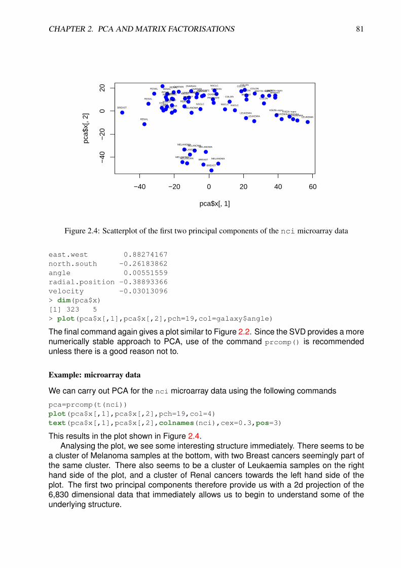
CHAPTER 2. PCA AND MATRIX FACTORISATIONS 81
●●●
●
● ●●
●
●
●
●●
●●● ● ●
●● ●
●
●
●
●
●●
●
●●●
● ●
●
●● ●
●●●●●
● ●
●●
● ●●
●●●●
●
● ●
●●
●
●
●
●●
●
●
−40 −20 0 20 40 60
−40
−20
020
pca$x[, 1]
pca$
x[, 2
]
CNSCNS
CNS
RENAL
BREASTCNS
CNSBREAST
NSCLC
NSCLC
RENAL
RENAL
RENALRENAL
RENAL RENALRENAL
BREAST
NSCLC RENAL
UNKNOWN
OVARIAN
MELANOMA
PROSTATE
OVARIANOVARIAN
OVARIAN
OVARIAN
OVARIANPROSTATENSCLC NSCLC
NSCLC
LEUKEMIAK562B−repro
K562A−reproLEUKEMIALEUKEMIA
LEUKEMIALEUKEMIALEUKEMIA
COLONCOLON
COLON
COLON
COLON COLON
COLON
MCF7A−reproBREAST
MCF7D−repro
BREAST
NSCLC
NSCLC NSCLC
MELANOMABREAST
BREAST
MELANOMA
MELANOMA
MELANOMAMELANOMA
MELANOMA
MELANOMA
Figure 2.4: Scatterplot of the first two principal components of the nci microarray data
east.west 0.88274167north.south -0.26183862angle 0.00551559radial.position -0.38893366velocity -0.03013096> dim(pca$x)[1] 323 5> plot(pca$x[,1],pca$x[,2],pch=19,col=galaxy$angle)
The final command again gives a plot similar to Figure 2.2. Since the SVD provides a morenumerically stable approach to PCA, use of the command prcomp() is recommendedunless there is a good reason not to.
Example: microarray data
We can carry out PCA for the nci microarray data using the following commands
pca=prcomp(t(nci))plot(pca$x[,1],pca$x[,2],pch=19,col=4)text(pca$x[,1],pca$x[,2],colnames(nci),cex=0.3,pos=3)
This results in the plot shown in Figure 2.4.Analysing the plot, we see some interesting structure immediately. There seems to be
a cluster of Melanoma samples at the bottom, with two Breast cancers seemingly part ofthe same cluster. There also seems to be a cluster of Leukaemia samples on the righthand side of the plot, and a cluster of Renal cancers towards the left hand side of theplot. The first two principal components therefore provide us with a 2d projection of the6,830 dimensional data that immediately allows us to begin to understand some of theunderlying structure.
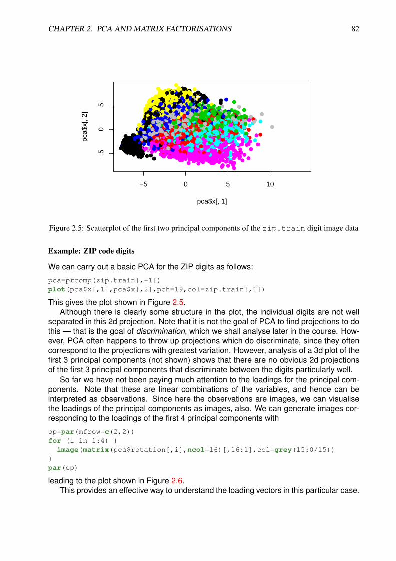
CHAPTER 2. PCA AND MATRIX FACTORISATIONS 82
●
●
●
●
●
●●
● ●
●
●●
●
●
●
●
●
●
●
●
●
●
●
●
●●
●
●
●
●
●
●
●
●
●
●●
●
●
●
●
●
●
●
●
● ●
●
●
●
● ●
●
●
●
●
●
●
●
●
●
●
●
●●
●●●
●
●●
●
●
●
●● ●
●
●
●
●
●
●
●
●
●
●
●●●
●
●
●
●
●
●
●
●
●
●
●
●
●
●
●
●
●
●
●
●
●
●
●
●
●
●
●
●●
●
●
●
●●●
●
●
●
●
●
●
●●
●
●
●
●
●
●
●
●
●
●
●●
●
● ●
●
●
●
●
●●
●
●
●
●
●
●
●
●
●
●
●
●
●●
●
●
●● ●
●
● ●●
●
●●
●
●
●
●●
●
●
● ●●
●
●
●
●
●
●
●●●
●
●
●
●
●
●
●
●
●●
●
●
●
●
●
●
●
●●
●●
●
●
●
●
●
●
●
●●
●
●
●
●
●
●
●●
●
●
●●
●●
●
●
●
●
●
●
●●
●
●●
●
●
●
●●
●
●
● ●
●
●
●
●
●
●
●
●
●
●
●
●
●
●
●
●
●
● ●
●
●
●
●
●
●
● ●
●
●
●
●
●
●
●
●
●
●●
●
●
●
●
●●●
●
●
●
●●
●
●●
●
●●
●
●
●
●
●
●
●
●●●
●●
●
●
●
● ●
●
●
●
●
● ●
●
●
●●
●
●
● ●
●
●
●
●●
●
●
● ●
●
●
●
●
●●
●
●●●
●
●●
●
●
●
●
●
●●
●●
●●
●
●
●
●
●
●
●
●
●
●
●
●
●
●
●
●
●
●
●
●
●
●
● ●●
●
●
● ●●
●
●●
●
●
●
●
●
●
●
●
●●
●
●
●
●
●
●
●
●
●
●
●
●
●
●
●
●
●●
●
●
●
●
●
●
●
●
●●
●
●
●
● ●
●
●
●
●
●
●
●
●
●
●
●
●●
●
●
●●
●
●
●
●
●●
●
●
●
●
●
● ●
●
●
●
●
●
●
●
●
●●
●
●●
●
●●
●●
●
●
●
●
●
●
●
●
●●
●
●●
●
●
●●
●
●
●
●●
●
●
●
●
●
●
●
●●●
●
●
●
●
● ●
●●
●
●
● ●
●●
●
●
●
●
●●
●
●
●
●
●
●
●●
●
●
●
●
●
●
●●●●
●
●
●● ●
●
●● ●
●
●
●
●
●
● ●
●
●
●
●
●
●●
● ●
●●
●●
●
●
●
●
●
●
●
●●
●
●
●
●
●
●●
●
●●
●
●●
●
●
●
●
●
●●
●
●
●
●
●●
●
●
●
●
●
●
●
●
●
●
●
●
●●●
●
●
●
●
●
●
●
●
●●
●
●
●
●●
●
●
●
●●
●
●
●
●
●●
●
●
●
●
●
●
●
●●
●
●
●
●
●●
●●
●
● ●
●
●●
●
●
● ●
●
● ●
●
●●
●
●
●
●
●
●
●●
●
●
●
●●
●
●
●
●
●
● ●
● ●
●
●
●●
●
●
●●●
●●
●
●
●
●
●
●
●
●
●
●
●
●
●
●
●
●
●
●
●
●
●
●
●
●
●●
●
●●
●●
●
●
●
●
●●
● ●
●
●
●
●
●
●
●
●
●
●
●
●
●●
●
●
●
●
●
●
●●●
●
●
●
●
●●
●
●
●●
●
●
● ●
●
●
●
●
●
●
●
●
●
●
● ●
●
●
●
●●
●
●●
●
●
●
●●
●●
●
●
●
●
●
●
●
●
●
●
● ●
●
●
●
●●
●
●
●
●●
●●
●
●
●
●
●
●
●
●
●
●●
●
●
●
●
●
●
●
●
●●
●
●
●
●
●
●
●
●
●
●
●
●
●
●
●
●●
●
●
●
●
●
●
●
●
●
●
●
●
●
●
●●
●
●
●
●
●
●
●●
●
●
● ●
●
●
●
●
●
●
●●
●●
●
●
●
●
●
●
●
●
●
●●
●
●
●
●
●
●
●
●
●
●
●
●
●●
●●
●
●
●
●
●
●
●
●
●●
●●
●
● ●
●
●
●
●
●
●
●●
●
●
●
●
●
●
●
●
● ●
●
●
●
●
●
●
●
●
●
●
● ●
●
●
●●
●
●
●
●●
●
●
● ●
●
●
●
●
● ●●
●
●
●
●
●
●
●
●
●●
●
●
●
● ●
●●
●
●
●●
●●
●
●
●
●
●
●
●
●
●
●
●
●
●
●
●
●
●
● ●
●
●
●
●
●
●
●
●
●
●
●
●
●
●
●
●
●●
●
●
●
●
●
●
●
●
●●
●
●
●
●
●●
●●
●
●
●
●
●●
●
● ●
●
●
●
●
●
●
●
●
●
●
●
●
●
●
●●
● ●
●●
●
●
●● ●●
●●
●
●
●
●
●
●
●
●●
●●●
●
●●
●
●
●●
●
●●
●
●
●
●
●
●●
●
● ●
●
●
●
●
●
●●●
●●
●●●
● ●
●
●
●
●
●
●
●
●●
●
●
●
●
●
●
●
●
●
●
●●
●
●
●
●
●
●
●
●
●
●
●
●●
●
●
●
●
●
●
●
●
●●
●
●
●
●
●
●
●
●
●
●
●
●
●
●
●●
●
●●
●
●
●
●●
●
●
●
●
●
●
●
●
●
●
●
●
●
●
●
●
●
●
●
●
●
●
●
●
●
●
●
●
●
●
●
●●
●
●
●●●
●
●
●
●
●
●●
●
●●
●
●●
●
●
●
●
●
●
●
●
●
●
●
●●
●●
●
●
● ●●
●●
●
●●
●
●
●●
●
●
●
●
●●
●
●
●
●
●
●
●
●
● ●
●●
●
●
●
● ●●●
●
●
●
●
●
●
●
●
●
●●●
●
●●
●
●
●
●
●
●●
●
●
●
●
●●
●
●
●
●●●
●
●
●
● ●
●
● ●
●
●
●
●●
●
●
●
●
●
●●
●
●
●●
●
●
●
●
●
●
● ●
●
●
●
●
●●
●●
●
●●
●
●
●
●
●
●
●
●
●
●
●●
●
●
●
●
●
●
●
●
●
●
●
●
●
●
● ●
●●
●
●
●
●
●
●
●
●
●●
●
●
●
●●
●
●
●
●●
●
●●
●
●
●
●
●
●
●●
●
●
●●
●
●●
●●
●
●
●●
●
●
●
●
●
●
●
●
●
●
●
●
●
●●●
●
●
●
●●
●
●●
●
●
●●●
●
●
●
●
●
●
●
●
●
●
●
●
●
●
●
●
●
●●
●
●
●
●
●
●
●
●
●
●
●
●
●● ●
●
●
●●●●
●
●
●
●●
●
●
●
●
●●
●
●●
●
●
●
●
●
●
●●
●
●
●
●
●● ●
●
●●
●
●●
●
●
●
●
●
●
●
●
●
●●
●
●
●●●●
●●
●
●
●
●
●
●
●
●
●
●
●
●
●●●
●●
●
●
●
●
●
●
●
●
●
●
●
●
●
●
●
●
●
●●●
●
●
●
● ●
●
●
●
●
●●●
●
●
●●
●
●
●●
●
●
●●
●
●
●
●
●
●
●
●
●
●
●
●
●
●●
●
●
●●
●
●
●
●
●
●
●
●
●
●
●
●
●
●●
●
●●
●
●●
●
● ●
●
●
●
●
●●●
●●●
●
●
●
●●
●
●
●●
●
●●
●
●●
●
●
●
●
●
● ●
●
●
●
●
●
●
●
●
●
●
●
● ●
●●
●
●
●
●
●
●
●
●
●
●●
●● ●
●
●
●
●
●
●
●●●
●
●
●
●●
●
●
●
●
●
●
●●●
●
●
●
●
●
●
●●
●●
●
●
●
●
●
●
●●
●
●
●
●
●
●
●●
●
●
●
●
●
●
●
●●●●
●
●
●●
●
●
●
●
●
●
●
●
●
●
●●
●
●
●●
●
●
●
●
●
●
● ●●
●
●
●
●●
●
●
●
●
●
●
●
●
●
●
●
●
●
●
●
●
●●
●
●●
●
●
●●
●
●
●
●●
●
●●
●
●
●
●
●●
●
●
●
●
●
●
●●
●
● ●
●
●
●
●
●
●●
●
●●
●
●
●
●
●
●
● ●
●●
●
●
●
●
●
●●
●
●
●
●●
●
●
●
●
●
●
●●
●
●
●
●
●
●
●
●
●
●
●
●
●
●
●
●
●
●
●
●
●
●
●●
●●
● ●
●
●
●
● ●●
●
●
●
●
●
●
●●●
●
●
●
●
●
●
●
●
●
●
●●
●●
●
●
●
●● ●
●
●
●
●
●
●
●●
●
●
●
●
●
●
●●
●
●
●
●●
●
●
●
●
●
●
●
●
●
●
●
●
●
●
●
●
●
●
●
●
●●
●
●●
●
●
●
●
●
●
●
●
●●
●
●
●
●
●
●
●
●●
●
●●
●
●
●
●
●
●
●
●
●
●
●●
●
●
●
●
●
●●
●
● ●
●●
●
●
●
●
● ●●●
●
●
●
●
●
●
●
●
●●
●
●
●
●
●
●
●
●
●
●
●
●
●
●
●
●
●
●
●
●●●
●
●
●
●
●
●
●
●
●
●
●
●
●
●
●
●
●
●
●
●
●
●
● ●
●
●
●
●
●
●●
●
●
●
●
●
●
●
●
●
●
●
●
●
●
●
●
●
● ●
●
●
●
●●
●●
● ●
●
●
● ●
●●
●
●
●
●●
●
●
●
●
●
●●●
●
●
● ●
●
●●
● ●
●
●
●
●●
●
●
●●
●
●
●
●
●
●
●
●
●
●●
●
●
●
●●
●
●
●●
●
●
●●
●
●●
●
●●
●
●
●
●
●
●
●●●
●
●
●●●
●
●
●
●
●
●
●●
●
●
●
●
●
●
●
●
●
●
●
●
●
●●
●
●
●
●
●
●
●
●
●●
●
●
●
●
●
● ●
●
●● ●
●
●
●
●
●
●
●
●
●
●
●
●
●
●
●
●
●
●
●
●
●●
●
●
●
●
●
● ●●
●
●
●
●●
●●
● ●
●
●
●
●
●
●
●
●
●
●
●
●
●
●
●●
●
●
●●
●
●
●
●
●
●
●
●
●
●
●●
● ●
●●
●
●
●
●
●
●●
●
●
●
●
●
●
●
●
●
●
●
●
●
●
●
●
●
●
●
●
●
●
●●
●
●
●
●●
●
●
●
●●
●
●
●
●
●
●
●
●
●
●
●
●
●
●
●
●●
●
●●
●
●
●
●
●
● ●
●
●
●
●
●
●
●
●●
●
●
●
●
●
●
●
●
●
●
●
●
●
●
●
●
●
●
●
●
● ●
●
●
●●
●
●
●
●
●
●●
●
●
●
●
●●
●
●
●●
●
●
●●
●
●
●●
●
●
●
●
●●
●
●
●
●
●●
●
●
●
●
●
●
●
●
●
●
●
●
●
●
●●
●
●
●
●●
●
●●
●●●
●
●
●
●
●
●
●
●
●●
●
●
●
●
●
●
● ●
●
●
●
●
●
●
●
●
●
●
●
●●
●
●
●
●
●
●
●●
●●
●
●
●
●
●
●●
●
●
●
●●
●
●
●
●
●●
●
●
●
●
●
●
●●
●
●
●●
● ●●
●
●
● ●●
●●
●
●
●
●
●
●
●
●
●
●
●
●
●
●
●
●
●
●● ●
●
●●
●
●
●
●
●
●
●●
●
●
●
●
●
●
●
●
●
●
●
●
●
●
●
●
●
● ●
●
●
●
●
●
●
●
●
●●
●
●
●
●
● ●
●
●
●
●●●
●
●
●
●
●
●
●
●
●
●
●
●
●
●
●
●
●●
●
●
●
●
●
●●
●
●
●
●
●
●
●
●
●
●●●
● ●
●●
●
●
●
●
●
●
●
●
●●
●
●
●
●
●
●
●
●
●●
●
●
●
●
●
●
●
●
●
●
●
●
●
●
●
●
●●
●
●
●
●
●●
●
●
●
●
●
●
●
●●
●
●
●
●●
●●
●
●●
●
●
●
●
●
●
●●
●
●●
●
●
●
●●
●●
●
●
●●
●
●
●
●●
●
●
●
●
●
● ●
●
●●
●
● ●
●
●
●
●●
●
●
●
●
●
●
●
● ●
●● ●●
●
● ●●
●● ● ●●●
●
●●
●
●●
●●
●
●
●
●●
●●●
●
●
●●
●
●
●
●●
●●
●●
●
●
●
●
●
●
●●
●
●
●
●
●
●●
●
●
●
●
●●
●
●
●
●
●
●●
●
●
●
●
●
●
●
●
●
●
●
●
●●
●
●
●●●
●
●●
●
●
●●
●
●●
●●
● ●
●
● ●●●
●●
●
●
●
●●
●
●
●
●
●
● ●●
●
●●
●
●●
●
●
●●
●
●
●
●●
●
●
●
●
●
●●
●
●
●
●
●
●●●
●
●
●
●
●
●
●
●
●
●
●
●
●
●
●
●●
●
●
●
●
●
●
●
●
●
●●
●●
●
●
●
●
●
●
●
●●
●
●
●
●
●
●
●
●●
●
●
●
●
●
●
●
●
●
●
●
● ●
●
●●
● ●
●
●
●
●
●
●
●
●
●●
●
●●
●
●
●
●
●
●●
●●
●
●
●
●
●
●
●
●
●
●
●
●
●
●
●
●
●
●●
●
●
●
●
●
● ●
●
●
●
●
●
●
●
●
●
●
●
●
●
●
●
●
●
●
●
●
●
●
●
●
●●
●
●
●●
●
●
●●
●● ●
●
● ●
●
●
●
●
●●
●
●
●
●●
●
●
●
●●●
●
●
●
●
●
●
●
●
●
● ●
● ●●
●
●
●
●
●
●
●
●
●
●
●
●
●
●
●
●
●
●
●
●
●
●
●
●
●
●
●
●
●
● ●
●
●
●●
●
●
●
●
●
●
●
●
●
●
●
●
●
●
●
●
●
●
●
●
●
●
●
●
●
●
●
●
●
●
●
●●
●
●
●
●
●
●●
●●
●
●
●●
●●
●
●●
●
●
●
●
●
●
●
●
●
●
●
●
●
●●
●
●
●
● ●●
●
●●
●
●
● ●
●●
●
●
●
●●
●●
●
●
●
●
●
●
●
●
●
● ●
●
●
●
●
● ●
●
●
●●
●
●
●
●
●
●
●
●
●
●
●●
●
●
●●
●
●
●
●
●
●
●
●
●●●
●
●●● ●
●
●
●
●
●● ●
●
●
●
●
●
●
●
●
●
●●
●
●●
●●
●●
●●
●
●
●
●●
●
●
●
●
●
●●
●
●
●
●
●
●
●
●●
●
●
●
●
●
●●
●
●●
●
●
●
●
●
●
●
●
●
●●
●
●
● ●●
●●
● ●
●
● ●
●
●
●
●
●●●
●●
●
●
●
●
●
●
●
●
●
●●●
●
●
●●
●
●
●●●
●
●
●
●
●
●
●
●
●
●
●
●
●
●
●
●
●●
●
●●
●
●
●
●●
●
●
●
●
●
●●
●
●
●
●
●
●
●
●
●●
●
●
●●
●
● ●
●
●
●
●
●
●●
●
●
●
●
●●●
●
●
●
●
●●
●
●
●
●● ●
●
●
●
●
●
●●
●●
●
●
●●
●●●
●
●●
●
●●
●
●
●
●
●
●
●●
●
●
●
●
●
●
●
●
●
●
●
●
●
●
●
●
●
●
● ●
●
●
●
●
●
●
●
●
●
●
●
●●
● ●
●
●
●
●
●
●●
●
●
●
●
●
●
●
●
●
●
●
●
●●●
●
●●
●
●
●
●
●
●●●
●
●●
●
●●●
●
●
●
●
●
●
●●
●
●
●
●
●
●
●
●●
●●
●
●●
●
●
●
●
●
●
●
●
●●
●● ●
●
●
●
●
●
●
●
●
●
●
●●
● ●
●
●
●
●●●
●
●
●
●
●
●●
●
●
●●
●
●
●
●
●
● ●●
●
●
●
●●
● ●
●
●
●
●●
●
●
●
●
●
●
●
●
●
●
● ●●
●
●
●
●
●●
●●●
●●
●
●
●●
●
●
●
●●
●
●
●
●
●●
●
●
●● ●●
●
●
●
●
●
●●
●●
●●
●
●
●
●
●●
●
●
●
●
●
●
●●
●● ●
●
●
●
●
●
●
●
●
●
●●
●
●●
●
● ●
●
●
●
●
●
●●
●
●
● ●●
●
●
●
●●●
●
●
●
●
●
●●
●
●
●
●●
●
●
●
●
●
●
●
●
●
●
●●
●● ●
●●
●●
●●
●
● ●
●●
●●
●
●●
● ●
●
●
●
●
●
●
●
●
●
●
●
●
●
● ●
●
● ●
●
●
●
●
●●
●
●
●
●
●
●●
●
●
●
●
●
●
●
●
●●
●
●
●
●
●
●●●
●●
●
●
●
●
●
●● ●
●
●●
●
●●
●
●
●
●
●
●
●
●●
●●
●
●
●●
●
●
●
●
●
●
●
●
●
●
●
●
●
●
●
●
●
●
●
●● ●
●
●
●
●●
●
●
●
●
●
●
●
●
●
●
●
●●
●
●
●
●
●
●
●●
●●
●
●
●●
●
●
●
●
●●
●
●●
●
● ●
●●
●
●
●
●
●
●
●
●
●
●
●
●
●
●
●
●
●
●
●●
●●
●
●
●
●
●
●
●
●
●
●
●●
●●●
●
●
●
●
●
●
●●
●
●
●
●
●
●
●
●
●
●
●
●
●
●
●●
●●●
●
●
●
●
●
●
●
●●●
●●
●●
●
●
●●
●
●
●
●
●
●
●
●●
●●
●
●
●
●
●
●
●
●
●
●
●
●
●
●
●
●
●●
●
●
●
●●
●●●
●
●
●
●
●
●
●
●
●
●
●
●
●●
●
●
●
●
●
●●
●
●
●
●
●
●
●
●●
●
●
●
●
●
●
●
●
●
●
●
●
●
●
●●
●
●
●
●
●●
●
●●
●
●
●
● ●
●
●
●
●
●
●
●
● ●
●
●
●
●
●
●
●
●
●
●●●
●
●
●
●
●
●
●
●
●
●
●
●
●
●●
●
●
●
●
●
●
●●
●
●
●
●
●
●●
●
●
●
●
●
●
●●
●●●
●●
●
●
●●
●
●
●
●
●●
●
●
●
●
●
●
●
●
●
●
●
●
●
●
●
●●
●
●
●
●●
●
●
●●
●
●
●
●
●
●●
●
●
●●
●
●
●●
●
●
●
●
●
●
●
● ●
●
●
●
●
●
●
●
●
●
●
●
●
● ●
●
●
● ●
●
●
●
●
●●
●
●
●
●●●
●●
●
●
●
●
●
●
●
●●
●
●
●
●
●●
●
●
●
●
●
●
●●
●
●●●
●●
●
●
●
●
●●
● ●
●●
●
●
●
●●
●●
●
●●
●
●
●
●
●
●
●
●
●
●
●
●●
●
●
●
●
●
●
●
●
●
●●
●
●
●●
● ●
●
●
●
●
●●
●
●●
●●●
●
●● ●●
● ●
●
●●
●
● ●
●●●
●
●
●
●
●
●
●
●
●
●●
●
●
●
●●
●●●
●●
●
●
●
●
●●
●
●
●
●●●
●
●●
●
●
●
●
●
●
●●
●
●
●
●●●
●● ●
●
●
●
●
●
●
●
● ●
●
●
●●
●
●●
●
●
●●
●
●
●●
●
●●
●
●
●
●●
●
●●
●●
●
●
●
●●
●
●
●●
●●
●
●
●
●
●
●
●●
●
● ●
●
●
●
●
●
●
●
●
●
●
●
●
●
●
●
●
●
●
●
●
●●
●
●
●
●
●
●
●
●
●● ●
●
●
●
●
●
●●
●
●
●
●
●
●●●
●
●
● ●
●
● ●
●
●
●
●
●●
●
●
●●
●●●
●
●
●
●
●
●
●
●
●● ●●
●
●
●
●●
●
●
●●
●
●
●
●
●
●
●
●
●
●
●
●
●
●
●
●
●
●
●●
●●
●
●
●
●
● ●
●
●●
●
●
●
●●
●
●
●
●●●
●
●
●
● ●
●
●●●
●●
●●
●
●
●●
●
●
●
●●
●
●
●
●●
●●●
●
●
●
● ●●
●●
●●
●●●
●
●
●
●
●
●● ●
●
●
●
●
●
●
●
●
●
●
●
●
●
●●
●
●
●
●
●
●
●
●
●
●
●●
●
●
●
●●●
●
●●
●
● ●
●
●●
●
●
●
●
●
●●
●
●●
●
● ●
●
●
●●
●
●●
●●
●
●
●
●
●●
●●●
●
●
●
●
●
●
●
●
●
● ●
●
●
●
●●
●
●
●
●
●
●
●●
●
●
●
●
●
●
●
●●
●
●
●
●
●
●
●●
●
●
●
●
●
●
●
●
●
●●
●
●
●
●●
●
●
●
●●
●
●
●
●
●
●
●
●
●
●
●●●
●
●●
●
●●●
●
●
●
●●
●
●
●
●
●
●
●
●
●
●
●
●●●
●●
●
●
●
●
●●●
●
●
●●
●
●
● ●●●
●
●
● ●
●
●●●
● ●
●
●
●
●
●
●
●
●
●●
●●
●
●●●
●
●
●
●●
●
● ●
●
●●
●
●
●
●
●
●
●
●
●●
●
●●
●●
●
●
●
●
●
●
●
●
●
●
●
●●
●
●
●
●●
●
●●
●
●●
●
●●
●●
●●
●●
● ●
●●
●●●
●
●
●
●
●●
●
●●
●
●
●
●
●
●
●
●
●
●
●
●
● ●
●
● ●
●
●
●
●
●
●
●
●
●
●
●
●●
●
●
●
●●
●
●
●
●
●
●
●
●
●
●
●
●
●
●
●
●
●
●
●
●
●
●●
●
●
●
●
●
●
●
●
●●
●●
●
●
●
●
●●
●●●●●
●
● ●●
●
●
●
●
●
●
●
●
●
●
●●
●●
●●
●
●
●
●
●
●
●
●
● ●
●●
●
●
●
●
●
●
●
●
●●
● ●
●
●
●
●
●●
●
●
●●
●
●
●
●
●●● ●
●
●
●
●
●●
●
●
●
●
●
●
●●●
●
●
●
●
●
●
●
●
●
●
●
●
●
●
●
●●
●
●
●
●●
●
●
●●
●
●
●
●
●
●●
●
●
●
●
●
●
●
●
● ●
●●
●
●
●
●
●
●●
●
●
●
●
●
●
●
●●●
●●
●
●
●
●
●
●
●
●
●
●
●
●
●
●
●
●
●
●
●● ●
●
●
●
●●
●
●
●
●
●●
●●●
●●
●
●
●
●
●
●
●●
●
●
●●
●
●
●
●
●
●
●
●
●●
●
●
●
●
●
●
●
●
●
●
●
●●
●
●
●
●
●
●
●
●
●
●
●
●●
●
●●
●
●
●
●
●
● ●
●●
●
●
●
●
●
●●
●
●
●
●
●
●
●
●●
●●
●
● ●●
●
●
●
●
●
●
●
●
●
●
●
●
●
●
●
●
●
●
●
●●
●
●●
●
●
●
●
●
●●
●
●
●
●●
●
●
●●
●
●
●
●
●
●
●
●
●
●
●●
●
●
●
●
●
●
●
●
●
●
●
●●
●
●
●
●● ●●
●
●
●
●
●
●●
●
●
●
●
● ●
●
●
●
●●
●
● ●
●
●
●
●
●
●
●
●●
●
●
●●
●
●
●
●
●
●●
●
●
●
●●
●
●●
●●
●
●
● ●
●
●●
●●
● ●
●
●
●
●
●
●
●
●
●●
●
●●
●
●
●
●
●
●
●
●
●
●
●●●
●
●
●●
●
●
●●
●
●
●
●●
●
●
● ●
●
●●
●
●
●
●
●
●
●
●
●
●
●
●
● ●
●
●
●
●
●●●
●
●●●
● ●●
●●
●
●
●
●
●
●
●
●
●
●
●
●
●
●
● ●
●
●
●
●
●
●
●
●●
●
●
●●●
●
●
●●●
●●
●
●
●
●●
●
●●
●
●●
●
●
●
●
●
●
●
●
●
●●
●
●
●●
●
●
●
●
●
●● ●
●
●
●
●
●
●●
●
●
●
●
●
●
●
●
●
●
●
●
●
●
●
●
●
●
●●
●
●
●
●
●
●
●
●
●
●
● ●●●
●
●
●
●
●●●
●
●
●
●
● ●
●
●
●
●
●●
●
●
●
●
●
●
●●
●
●
●
●
●
● ●
●
●
●
●
●
●●
●
●
●
●
●
●
●●
●
●
●
●
●
●
●
●●
●
●
●●●
● ●
●
●
●
●
●
●
●
●
●
●
●
●
●●
●
●
●
●
●
●
● ●
●●
●
●
●
●
●
●
●
●
●
●
●
●●
●
●
●●
●
●
●
●
●
●
●
●
●
●
●
●
●
●
●●
●●●
●
●
●
●●
●●
●
●
●
●
●
●
●
●
●
●
●
●
●
●
●
●
●
●
●
●
●
●
●●●●
●●
●
●
●
●
●
●
● ●
●
●
●
●
●
●
●
●
●
●●
●
●
●
●
●●
●
●
●
●●
●
●
●
●
●
●
●
●●
●
●●
●
●
●
●
●
●
●
●
●
●
●
●
●●
●●
●
●
●
●
●
●●
●●
●
●●
●
●●
●
●
● ●
●
●
●
●
●
●
●
●●
●●
● ●
●●
●
●
● ●
●
●
●
●
●●
●
●
●
●● ●
● ●●
●
●
●
●
●
●
−5 0 5 10
−5
05
pca$x[, 1]
pca$
x[, 2
]
Figure 2.5: Scatterplot of the first two principal components of the zip.train digit image data
Example: ZIP code digits
We can carry out a basic PCA for the ZIP digits as follows:
pca=prcomp(zip.train[,-1])plot(pca$x[,1],pca$x[,2],pch=19,col=zip.train[,1])
This gives the plot shown in Figure 2.5.Although there is clearly some structure in the plot, the individual digits are not well
separated in this 2d projection. Note that it is not the goal of PCA to find projections to dothis — that is the goal of discrimination, which we shall analyse later in the course. How-ever, PCA often happens to throw up projections which do discriminate, since they oftencorrespond to the projections with greatest variation. However, analysis of a 3d plot of thefirst 3 principal components (not shown) shows that there are no obvious 2d projectionsof the first 3 principal components that discriminate between the digits particularly well.
So far we have not been paying much attention to the loadings for the principal com-ponents. Note that these are linear combinations of the variables, and hence can beinterpreted as observations. Since here the observations are images, we can visualisethe loadings of the principal components as images, also. We can generate images cor-responding to the loadings of the first 4 principal components with
op=par(mfrow=c(2,2))for (i in 1:4) {image(matrix(pca$rotation[,i],ncol=16)[,16:1],col=grey(15:0/15))
}par(op)
leading to the plot shown in Figure 2.6.This provides an effective way to understand the loading vectors in this particular case.
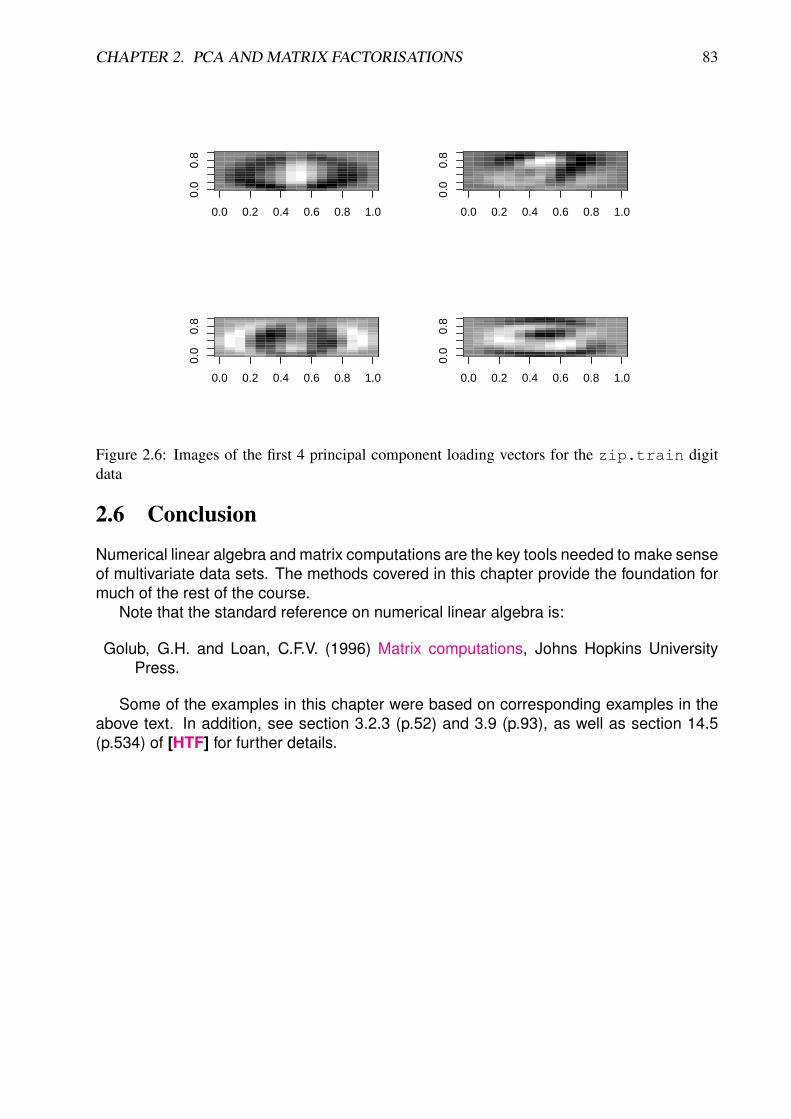
CHAPTER 2. PCA AND MATRIX FACTORISATIONS 83
0.0 0.2 0.4 0.6 0.8 1.0
0.0
0.8
0.0 0.2 0.4 0.6 0.8 1.0
0.0
0.8
0.0 0.2 0.4 0.6 0.8 1.0
0.0
0.8
0.0 0.2 0.4 0.6 0.8 1.0
0.0
0.8
Figure 2.6: Images of the first 4 principal component loading vectors for the zip.train digitdata
2.6 Conclusion
Numerical linear algebra and matrix computations are the key tools needed to make senseof multivariate data sets. The methods covered in this chapter provide the foundation formuch of the rest of the course.
Note that the standard reference on numerical linear algebra is:
Golub, G.H. and Loan, C.F.V. (1996) Matrix computations, Johns Hopkins UniversityPress.
Some of the examples in this chapter were based on corresponding examples in theabove text. In addition, see section 3.2.3 (p.52) and 3.9 (p.93), as well as section 14.5(p.534) of [HTF] for further details.
Chapter 3
Inference, the MVN and multivariateregression
3.1 Inference and estimation
So far we have considered the analysis of data matrices X, including the computation ofthe sample mean vector x and variance matrix SX. We have also considered randomvectors X, including the expectation vector E(X) and variance matrix Var(X). How-ever, although we have informally noted a relationship between sample and populationquantities, we have not yet formally established a connection between the two.
Proposition 21 Suppose that we form an n×p data matrix X with rowsX iT, i = 1, 2, . . . , n
where theX i are independent realisations of a multivariate random quantity with E(X i) =µ and Var(X i) = Σ. Assuming that the elements of µ and Σ are all finite, we have thefollowing:
1. The sample mean X is unbiased for µ, that is
E(X)
= µ.
2. The variance of X is given by
Var(X)
=1
nΣ.
3. X is a consistent estimator of µ, that is
P(‖X − µ‖ < ε
) n−→∞
1, ∀ε > 0.
4. The sample variance SX is unbiased for Σ, that is
E(SX) = Σ.
Before demonstrating these results, it should be noted that under some additional (fairlymild) assumptions it can be shown that the sample variance matrix is also a consistentestimator of Σ, but we will not pursue this here.
84

CHAPTER 3. INFERENCE, THE MVN AND MULTIVARIATE REGRESSION 85
Proof
1.
E(X)
= E
(1
n
n∑i=1
X i
)
=1
n
n∑i=1
E(X i)
=1
n
n∑i=1
µ
= µ.
2.
Var(X)
= Var
(1
n
n∑i=1
X i
)
=1
n2
n∑i=1
Var(X i)
=1
n2
n∑i=1
Σ
=1
nΣ.
3. Consistency is intuitively obvious, since 1. and 2. tell us that E(X)→ µ and
Var(X)→ 0 as n → ∞. However, we can establish consistency more formally
by applying Markov’s inequality to ‖X − µ‖2. First note that
‖X − µ‖2 = (X − µ)T(X − µ) =
p∑i=1
(Xi − µi)2 ≥ 0.

CHAPTER 3. INFERENCE, THE MVN AND MULTIVARIATE REGRESSION 86
Now we have
E(‖X − µ‖2
)= E
(p∑i=1
(Xi − µi)2)
=
p∑i=1
E((Xi − µi)2
)=
p∑i=1
Var(Xi
)=
p∑i=1
1
nVar(Xi)
=1
nTr (Σ) .
Then Markov’s inequality tells us that for any a > 0 we have
P(‖X − µ‖2 ≥ a
)≤ Tr (Σ)
na
⇒ P(‖X − µ‖2 < a
)≥ 1− Tr (Σ)
na
and putting a = ε2 we get
P(‖X − µ‖2 < ε2
)≥ 1− Tr (Σ)
nε2
⇒ P(‖X − µ‖ < ε
)≥ 1− Tr (Σ)
nε2n−→∞
1.
4. First note that
E(SX) = E
(1
n− 1
n∑i=1
[X i − X][X i − X]T
)
=1
n− 1
n∑i=1
E([X i − X][X i − X]T
)Now since
E(X i − X
)= µ− 1
n
n∑i=1
µ = 0
CHAPTER 3. INFERENCE, THE MVN AND MULTIVARIATE REGRESSION 87
we have
E([X i − X][X i − X]T
)= Var
(X i − X
)= Var
(n− 1
nX i −
1
n
∑j 6=i
Xj
)
=(n− 1)2
n2Var(X i) +
1
n2
∑j 6=i
Var(Xj)
=(n− 1)2
n2Σ +
n− 1
n2Σ
=n− 1
nΣ,
and so
E(SX) =1
n− 1
n∑i=1
n− 1
nΣ = Σ.
�
These results now make explicit the relationship between the data summaries andassociated population quantities, and give us confidence that, at least in the case of“large n”, our sample summary statistics should be “good” estimators of the correspondingsummaries for the population from which the data is sampled.
3.2 Multivariate regression
In this section we will examine the problem of regression for a multivariate observation.We shall begin by reminding ourselves about multiple regression for a univariate outputas a “least squares” procedure, before going on to see how this can be generalised tothe case of multivariate output. Key to understanding regression as a “least squares”problem is the idea of minimising an error function with respect to a vector (or matrix)of parameters. There are various ways to approach this problem, but often the simplestis to use calculus to find a stationary point of the cost function (by differentiating wrt theparameters and equating to zero). For this purpose it is helpful to use some results ondifferentiating various scalar functions with respect to vector and matrix parameters. Westate the following results without proof.∗
Proposition 22 (Derivatives wrt vectors and matrices) In each of the following results,the derivative is of a scalar function, and is wrt a vector x or matrix X, where the compo-nents of the vector or matrix are assumed to be algebraically independent.
1.∂
∂xaTx =
∂
∂xxTa = a
∗The results can all be found in The Matrix Cookbook, to which you are referred for further details and many otherinteresting results and examples. Note that you are not expected to memorise these results, and their derivations arenot examinable in this course.
CHAPTER 3. INFERENCE, THE MVN AND MULTIVARIATE REGRESSION 88
2.∂
∂xxTAx = (A + AT)x
and note that this reduces to 2Ax when A is symmetric.
3.∂
∂XTr (XA) = AT
4.∂
∂XTr(XTAX
)= AX + ATX
and note that this reduces to 2AX when A is symmetric.
5.∂
∂XTr(XTAXB
)=
∂
∂XTr(BXTAX
)= AXB + ATXBT
and note that this reduces to 2AXB when both A and B are symmetric.
6.∂
∂X|X| = |X|X−T
7.∂
∂Xlog |X| = X−T
8.∂
∂XaTXb = abT
9.∂
∂XaTX−1b = −X−TabTX−T
Now we have the necessary technical results, we can think about the regression problem.
3.2.1 Univariate multiple linear regression
Let’s start with classical multiple linear regression where we model each output yi as alinear combination of a corresponding covariate vector xi, subject to error, as
yi = xiTβ + εi, i = 1, 2, . . . , n.
We assume that the covariates are the rows of an n × p data matrix X, and so β is ap-dimensional vector. We can write this in matrix form as
y = Xβ + ε.
Since we typically consider the case n > p, the presence of the error term ε is necessary,otherwise the system would be over-determined, and then typically no β would exist inorder to solve the linear system
y = Xβ.

CHAPTER 3. INFERENCE, THE MVN AND MULTIVARIATE REGRESSION 89
However, by introducing ε, we ensure that every β is a potential solution, for an appropri-ate choice of ε. The least squares approach is to choose the β which makes the 2-normof ε as small as possible. That is, we choose β in order to minimise
‖ε‖2 = εTε =n∑i=1
ε2i .
We can find such a minimising solution by first noting that
εTε = (y − Xβ)T(y − Xβ)
= yTy − 2yTXβ + βTXTXβ,
and then differentiate wrt β as
∂
∂βεTε = −2XTy + 2XTXβ.
Here we have used results 1. and 2. of Proposition 22. Then equating to zero leads to the“normal equations”
XTXβ = XTy.
The mathematical solution to this is
β = (XTX)−1XTy,
but there are very efficient and numerically stable ways to compute this based on matrixdecompositions such as the QR factorisation, as discussed in Section 2.4.2.
Example: galaxy data
Suppose that we would like to use the variables angle and radial.position in order topredict the variable velocity. We can accomplish this in R using the built-in commandlm(), either using R model notation, as
> lm(velocity∼ angle+radial.position,data=galaxy)
Call:lm(formula = velocity ∼ angle + radial.position, data = galaxy)
Coefficients:(Intercept) angle radial.position1586.9882 0.1076 2.4515
or just using vectors and matrices, as
> lm(galaxy[,5]∼ as.matrix(galaxy[,3:4]))
Call:lm(formula = galaxy[, 5] ∼ as.matrix(galaxy[, 3:4]))
Coefficients:(Intercept)
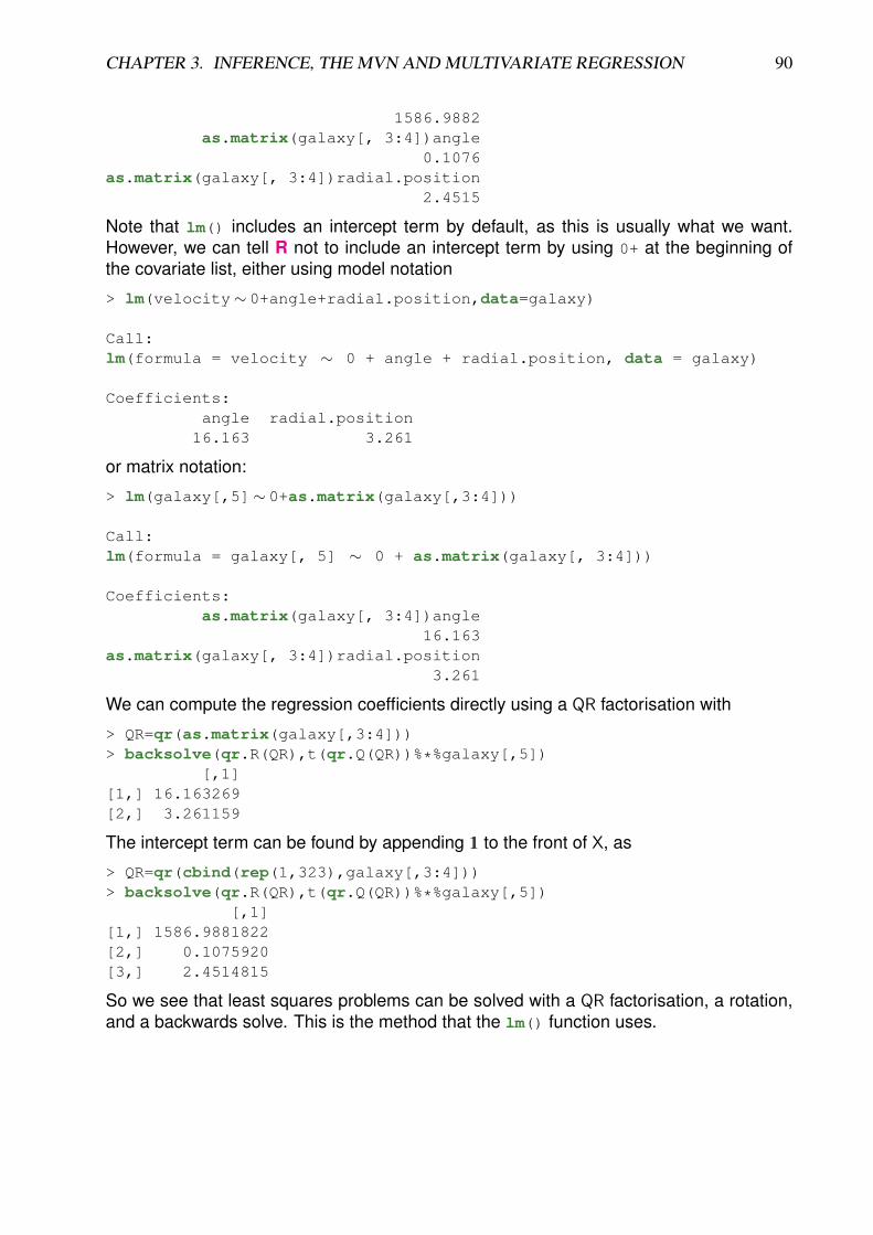
CHAPTER 3. INFERENCE, THE MVN AND MULTIVARIATE REGRESSION 90
1586.9882as.matrix(galaxy[, 3:4])angle
0.1076as.matrix(galaxy[, 3:4])radial.position
2.4515
Note that lm() includes an intercept term by default, as this is usually what we want.However, we can tell R not to include an intercept term by using 0+ at the beginning ofthe covariate list, either using model notation
> lm(velocity∼ 0+angle+radial.position,data=galaxy)
Call:lm(formula = velocity ∼ 0 + angle + radial.position, data = galaxy)
Coefficients:angle radial.position16.163 3.261
or matrix notation:
> lm(galaxy[,5]∼ 0+as.matrix(galaxy[,3:4]))
Call:lm(formula = galaxy[, 5] ∼ 0 + as.matrix(galaxy[, 3:4]))
Coefficients:as.matrix(galaxy[, 3:4])angle
16.163as.matrix(galaxy[, 3:4])radial.position
3.261
We can compute the regression coefficients directly using a QR factorisation with
> QR=qr(as.matrix(galaxy[,3:4]))> backsolve(qr.R(QR),t(qr.Q(QR))%*%galaxy[,5])
[,1][1,] 16.163269[2,] 3.261159
The intercept term can be found by appending 11 to the front of X, as
> QR=qr(cbind(rep(1,323),galaxy[,3:4]))> backsolve(qr.R(QR),t(qr.Q(QR))%*%galaxy[,5])
[,1][1,] 1586.9881822[2,] 0.1075920[3,] 2.4514815
So we see that least squares problems can be solved with a QR factorisation, a rotation,and a backwards solve. This is the method that the lm() function uses.

CHAPTER 3. INFERENCE, THE MVN AND MULTIVARIATE REGRESSION 91
3.2.2 The general linear model
Now consider the obvious generalisation of the previous case, where our “output”, yi isnow a q-vector, rather than a scalar. We then have the model
yi = BTxi + εi, i = 1, 2, . . . n,
where B is now a p× q matrix. We can write this in matrix form as
Y = XB + E,
where E is an n × q matrix of “errors”, and this is typically known as the general linearmodel. The regression problem here is, given data matrices X and Y, to find the matrix Bwhich makes the Frobenius norm of the error matrix, ‖E‖, as small as possible. Note that
‖E‖2 = Tr(ETE
)=
n∑i=1
q∑j=1
ε2ij,
and so this is again a least squares problem, where we choose B to minimise the sum ofsquares of the errors.
We proceed as before by noting that
Tr(
ETE)
= Tr([Y − XB]T[Y − XB]
)= Tr
(YTY − YTXB− BTXTY + BTXTXB
)= Tr
(YTY
)− Tr
(YTXB
)− Tr
(BTXTY
)+ Tr
(BTXTXB
)= Tr
(YTY
)− 2 Tr
(YTXB
)+ Tr
(BTXTXB
).
Now differentiating wrt the matrix B we get
∂
∂BTr(
ETE)
= −2XTY + 2XTXB,
where here we used results 3. and 4. of Proposition 22.Equating to zero gives a matrix version of the normal equations,
XTXB = XTY.
This has mathematical solutionB = (XTX)−1XTY.
By considering the columns of B and Y, we see that this corresponds to the usual multiplelinear regression solution for each column of Y. That is, the multivariate regression prob-lem is solved by separately regressing each column of Y on the data matrix X. However,the full problem will be solved more efficiently and stably by directly solving the abovenormal equations using a QR factorisation of X (with multiple RHSs). To be clear, if we
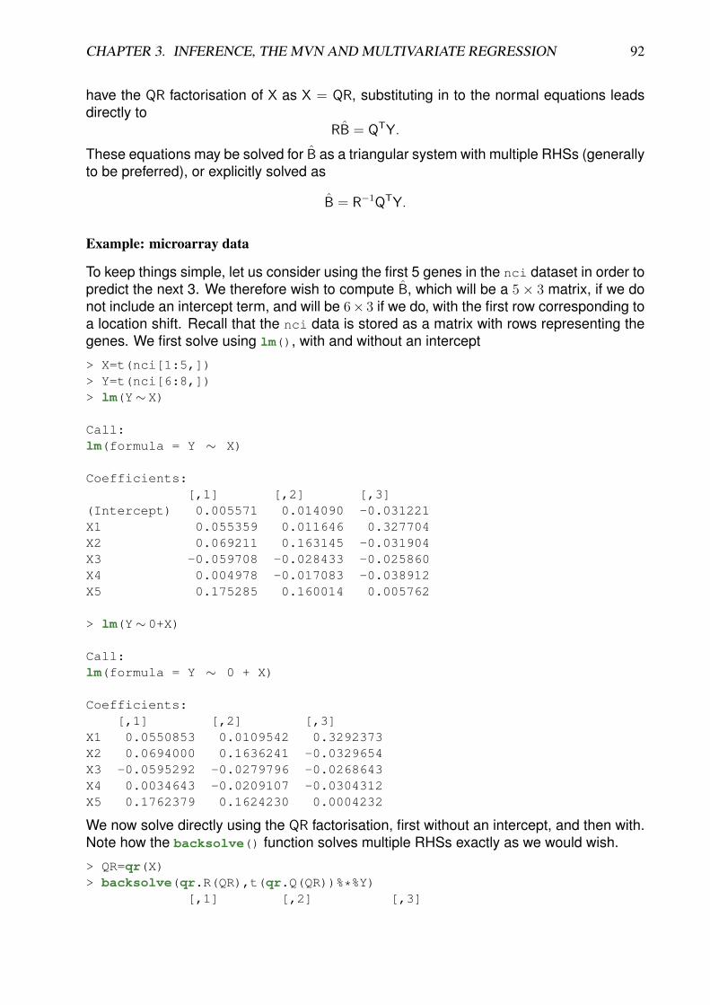
CHAPTER 3. INFERENCE, THE MVN AND MULTIVARIATE REGRESSION 92
have the QR factorisation of X as X = QR, substituting in to the normal equations leadsdirectly to
RB = QTY.
These equations may be solved for B as a triangular system with multiple RHSs (generallyto be preferred), or explicitly solved as
B = R−1QTY.
Example: microarray data
To keep things simple, let us consider using the first 5 genes in the nci dataset in order topredict the next 3. We therefore wish to compute B, which will be a 5× 3 matrix, if we donot include an intercept term, and will be 6× 3 if we do, with the first row corresponding toa location shift. Recall that the nci data is stored as a matrix with rows representing thegenes. We first solve using lm(), with and without an intercept
> X=t(nci[1:5,])> Y=t(nci[6:8,])> lm(Y∼ X)
Call:lm(formula = Y ∼ X)
Coefficients:[,1] [,2] [,3]
(Intercept) 0.005571 0.014090 -0.031221X1 0.055359 0.011646 0.327704X2 0.069211 0.163145 -0.031904X3 -0.059708 -0.028433 -0.025860X4 0.004978 -0.017083 -0.038912X5 0.175285 0.160014 0.005762
> lm(Y∼ 0+X)
Call:lm(formula = Y ∼ 0 + X)
Coefficients:[,1] [,2] [,3]
X1 0.0550853 0.0109542 0.3292373X2 0.0694000 0.1636241 -0.0329654X3 -0.0595292 -0.0279796 -0.0268643X4 0.0034643 -0.0209107 -0.0304312X5 0.1762379 0.1624230 0.0004232
We now solve directly using the QR factorisation, first without an intercept, and then with.Note how the backsolve() function solves multiple RHSs exactly as we would wish.
> QR=qr(X)> backsolve(qr.R(QR),t(qr.Q(QR))%*%Y)
[,1] [,2] [,3]
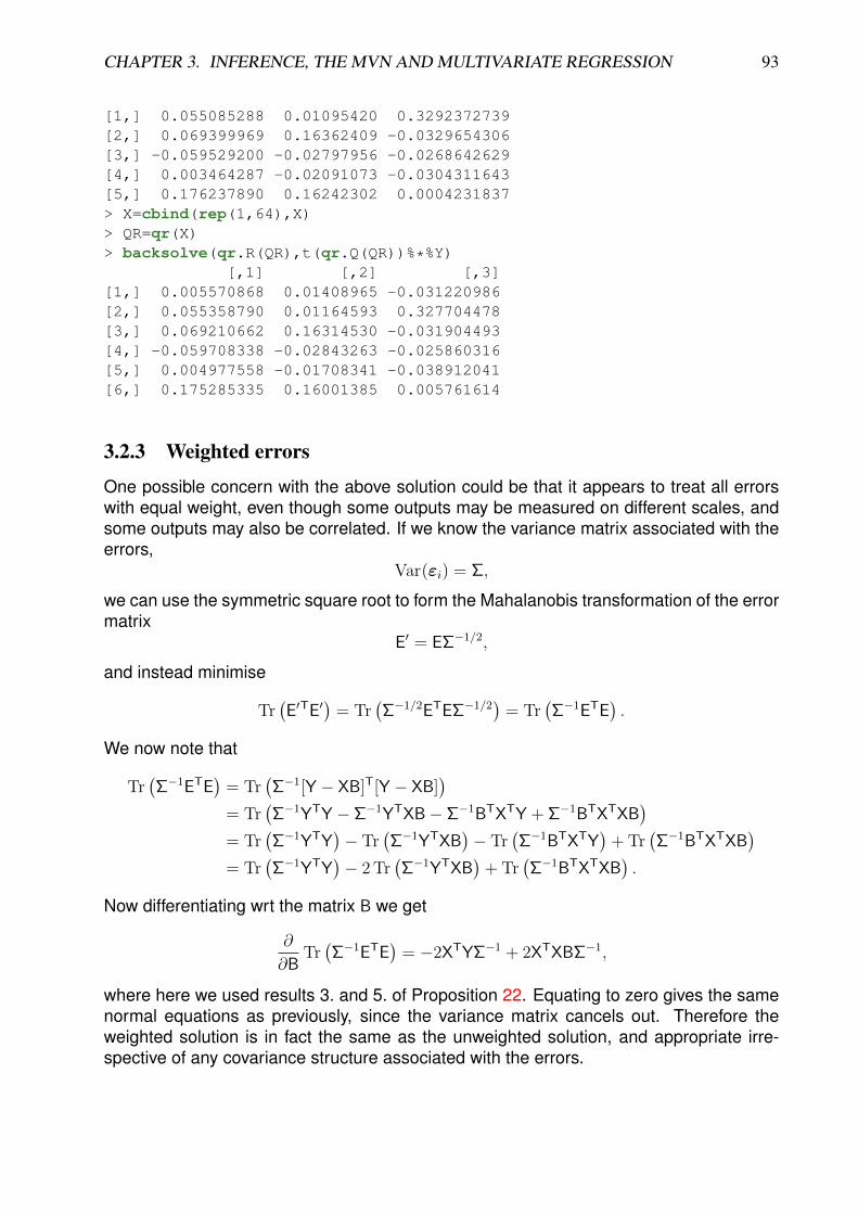
CHAPTER 3. INFERENCE, THE MVN AND MULTIVARIATE REGRESSION 93
[1,] 0.055085288 0.01095420 0.3292372739[2,] 0.069399969 0.16362409 -0.0329654306[3,] -0.059529200 -0.02797956 -0.0268642629[4,] 0.003464287 -0.02091073 -0.0304311643[5,] 0.176237890 0.16242302 0.0004231837> X=cbind(rep(1,64),X)> QR=qr(X)> backsolve(qr.R(QR),t(qr.Q(QR))%*%Y)
[,1] [,2] [,3][1,] 0.005570868 0.01408965 -0.031220986[2,] 0.055358790 0.01164593 0.327704478[3,] 0.069210662 0.16314530 -0.031904493[4,] -0.059708338 -0.02843263 -0.025860316[5,] 0.004977558 -0.01708341 -0.038912041[6,] 0.175285335 0.16001385 0.005761614
3.2.3 Weighted errors
One possible concern with the above solution could be that it appears to treat all errorswith equal weight, even though some outputs may be measured on different scales, andsome outputs may also be correlated. If we know the variance matrix associated with theerrors,
Var(εi) = Σ,
we can use the symmetric square root to form the Mahalanobis transformation of the errormatrix
E′ = EΣ−1/2,
and instead minimise
Tr(E′TE′
)= Tr
(Σ−1/2ETEΣ−1/2
)= Tr
(Σ−1ETE
).
We now note that
Tr(Σ−1ETE
)= Tr
(Σ−1[Y − XB]T[Y − XB]
)= Tr
(Σ−1YTY − Σ−1YTXB− Σ−1BTXTY + Σ−1BTXTXB
)= Tr
(Σ−1YTY
)− Tr
(Σ−1YTXB
)− Tr
(Σ−1BTXTY
)+ Tr
(Σ−1BTXTXB
)= Tr
(Σ−1YTY
)− 2 Tr
(Σ−1YTXB
)+ Tr
(Σ−1BTXTXB
).
Now differentiating wrt the matrix B we get
∂
∂BTr(Σ−1ETE
)= −2XTYΣ−1 + 2XTXBΣ−1,
where here we used results 3. and 5. of Proposition 22. Equating to zero gives the samenormal equations as previously, since the variance matrix cancels out. Therefore theweighted solution is in fact the same as the unweighted solution, and appropriate irre-spective of any covariance structure associated with the errors.
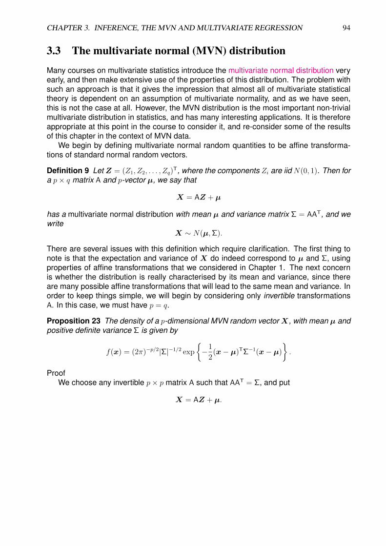
CHAPTER 3. INFERENCE, THE MVN AND MULTIVARIATE REGRESSION 94
3.3 The multivariate normal (MVN) distribution
Many courses on multivariate statistics introduce the multivariate normal distribution veryearly, and then make extensive use of the properties of this distribution. The problem withsuch an approach is that it gives the impression that almost all of multivariate statisticaltheory is dependent on an assumption of multivariate normality, and as we have seen,this is not the case at all. However, the MVN distribution is the most important non-trivialmultivariate distribution in statistics, and has many interesting applications. It is thereforeappropriate at this point in the course to consider it, and re-consider some of the resultsof this chapter in the context of MVN data.
We begin by defining multivariate normal random quantities to be affine transforma-tions of standard normal random vectors.
Definition 9 Let Z = (Z1, Z2, . . . , Zq)T, where the components Zi are iid N(0, 1). Then for
a p× q matrix A and p-vector µ, we say that
X = AZ + µ
has a multivariate normal distribution with mean µ and variance matrix Σ = AAT, and wewrite
X ∼ N(µ,Σ).
There are several issues with this definition which require clarification. The first thing tonote is that the expectation and variance of X do indeed correspond to µ and Σ, usingproperties of affine transformations that we considered in Chapter 1. The next concernis whether the distribution is really characterised by its mean and variance, since thereare many possible affine transformations that will lead to the same mean and variance. Inorder to keep things simple, we will begin by considering only invertible transformationsA. In this case, we must have p = q.
Proposition 23 The density of a p-dimensional MVN random vectorX, with mean µ andpositive definite variance Σ is given by
f(x) = (2π)−p/2|Σ|−1/2 exp
{−1
2(x− µ)TΣ−1(x− µ)
}.
ProofWe choose any invertible p× p matrix A such that AAT = Σ, and put
X = AZ + µ.
CHAPTER 3. INFERENCE, THE MVN AND MULTIVARIATE REGRESSION 95
We first need to know the probability density function for Z, which is clearly given by
φ(z) =
p∏i=1
φ(zi)
=
p∏i=1
1√2π
exp{−z2i /2}
= (2π)−p/2 exp
{−1
2
p∑i=1
z2i
}
= (2π)−p/2 exp
{−1
2zTz
}.
Now since X is an invertible transformation of Z, it’s density is given by
f(x) = φ(z)
∣∣∣∣∂z∂x∣∣∣∣ ,
where z = A−1(x− µ). But now∂z
∂x= A−1,
and so ∣∣∣∣∂z∂x∣∣∣∣ = |A−1| = |A|−1 = |Σ|−1/2,
giving
f(x) = (2π)−p/2 exp
{−1
2[A−1(x− µ)]T[A−1(x− µ)]
}|Σ|−1/2
= (2π)−p/2|Σ|−1/2 exp
{−1
2(x− µ)TΣ−1(x− µ)
}.
�
The crucial thing to note here is that despite the fact that we considered any (invertible) Aleading to a required variance matrix, the density of the resulting random quantity dependsonly on the variance matrix (and mean vector), and not on the particular affine transforma-tion used in the construction. Consideration of non-invertible (and non-square) transfor-mations complicates the analysis, but essentially the same conclusion holds, which is thatthe distribution of the MVN random quantity depends only on its mean and variance, andnot on the particular affine transformation used to construct it. It is therefore reasonableto characterise MVN random quantities by their mean and variance.
3.3.1 Evaluation of the MVN density
In some applications it is necessary to evaluate the MVN density. However, in most ap-plications, it is sufficient to evaluate the log of the density, and this is usually safer, as it isless susceptible to numerical underflow. Clearly the log-density is given by
l(x) = −p2
log 2π − 1
2log |Σ| − 1
2(x− µ)TΣ−1(x− µ).

CHAPTER 3. INFERENCE, THE MVN AND MULTIVARIATE REGRESSION 96
Note that the final term is essentially the Mahalanobis distance. We can avoid directcomputation of |Σ| and Σ−1 by using an appropriate matrix decomposition. In the positivedefinite case, the Cholesky decomposition usually provides the best solution, so supposethat Σ has Cholesky decomposition
Σ = GGT,
where G is lower triangular. To see how this helps, first consider the determinant term
1
2log |Σ| = log |Σ|1/2 = log |G|.
But since G is lower triangular, its determinant is the product of its diagonal elements, andso the log of this is given by
log |G| =p∑i=1
log gii.
Similarly, the final quadratic form can be simplified as
(x− µ)TΣ−1(x− µ) = (x− µ)T(GGT)−1(x− µ)
= (x− µ)TG−TG−1(x− µ)
= zTz,
where z = G−1(x−µ), and hence may be found by forward solving the triangular system
Gz = (x− µ).
Given this solution, we can therefore write the log density as
l(x) = −p2
log 2π −p∑i=1
log gii −1
2
p∑i=1
z2i .
This is an efficient way to compute the log density, as it just requires a Cholesky decom-position and a single forward solve.
3.3.2 Properties of the MVN
We now consider some very useful properties of the MVN distribution.
Proposition 24 (Affine transformation) If X ∼ N(µ,Σ), and
Y = AX + b,
then Y is multivariate normal, and Y ∼ N(Aµ+ b,AΣAT).
ProofThe mean and variance of Y are clear from our understanding of affine transforma-
tions of random vectors. The key to this result is understanding why Y is MVN. For this,

CHAPTER 3. INFERENCE, THE MVN AND MULTIVARIATE REGRESSION 97
note that we need to show that Y is an affine transformation of a standard normal vector,but since X is MVN, there must exist a matrix M such that
X = MZ + µ,
where Z is a standard normal vector. Then
Y = AX + b
= A(MZ + µ) + b
= (AM)Z + (Aµ+ b),
and so Y is also an affine transformation of a standard normal vector, and hence MVN.�
Now since marginal distributions correspond to linear transformations, it follows that allmarginal distributions of the MVN are (multivariate) normal.
Proposition 25 If X ∼ N(µ,Σ) is partitioned as(X1
X2
)∼ N
((µ1
µ2
),
(Σ11 Σ12
Σ21 Σ22
)),
then the marginal distribution of X1 is given by
X1 ∼ N(µ1,Σ11).
ProofThe result follows simply by noting that
X1 = (I, 0)
(X1
X2
),
and using properties of linear transformations. �
Similarly, univariate marginals my be computed using the fact that Xi = eiTX, giving
Xi ∼ N(µi, σii).
Proposition 26 If X1 ∼ N(µ1,Σ1) and X2 ∼ N(µ2,Σ2) are independent, then
X1 +X2 ∼ N(µ1 + µ2,Σ1 + Σ2).
Proof
First note that X1 and X2 are jointly MVN, with(X1
X2
)∼ N
((µ1
µ2
),
(Σ1 0
0 Σ2
)).
Then observing that X1 +X2 corresponds to the linear trans-formation
(I, I)
(X1
X2
)
CHAPTER 3. INFERENCE, THE MVN AND MULTIVARIATE REGRESSION 98
leads directly to the result.�
Finally, we state without proof the key result concerning conditional distributions of theMVN. The proof is straightforward, but somewhat involved.
Proposition 27 If X ∼ N(µ,Σ) is partitioned as(X1
X2
)∼ N
((µ1
µ2
),
(Σ11 Σ12
Σ21 Σ22
)),
then the conditional distribution of X1 given that X2 is observed to be x2 is MVN, with
(X1|X2 = x2) ∼ N(µ1|2,Σ1|2),
where
µ1|2 = µ1 + Σ12Σ22−1(x2 − µ2),
Σ1|2 = Σ11 − Σ12Σ22−1Σ21.
Note that the simple version of the result presented here assumes that Σ22 is invertible,but it generalises straightforwardly to the case of singular Σ22.
3.3.3 Maximum likelihood estimation
If we consider an n × p data matrix X with iid rows X i ∼ N(µ,Σ), then the likelihood foran observed data matrix is given by
L(µ,Σ; X) =n∏i=1
f(xi)
=n∏i=1
(2π)−p/2|Σ|−1/2 exp
{−1
2(xi − µ)TΣ−1(xi − µ)
}
= (2π)−np/2|Σ|−n/2 exp
{−1
2
n∑i=1
(xi − µ)TΣ−1(xi − µ)
}.
Consequently, the log-likelihood is given by
l(µ,Σ; X) = −np2
log 2π − n
2log |Σ| − 1
2
n∑i=1
(xi − µ)TΣ−1(xi − µ).
Note that if we need to numerically compute this log-likelihood, we would do so usingthe Cholesky decomposition, as already described for the log-density. We can use thelog-likelihood in order to compute maximum likelihood estimators for the MVN.
Proposition 28 For an MVN model, the maximum likelihood estimator of the mean, µ isgiven by
µ = x.

CHAPTER 3. INFERENCE, THE MVN AND MULTIVARIATE REGRESSION 99
ProofWe proceed by differentiating the log-likelihood function wrt µ and equating to zero.
First note that∂l
∂µ= −1
2
n∑i=1
∂
∂µ(xi − µ)TΣ−1(xi − µ).
Now
∂
∂µ(xi − µ)TΣ−1(xi − µ) =
∂
∂µ(xi
TΣ−1xi − 2µTΣ−1xi + µTΣ−1µ)
= −2Σ−1xi + 2Σ−1µ
= 2Σ−1(µ− xi),
using properties 1. and 2. of Proposition 22. So now
∂l
∂µ= −1
2
n∑i=1
2Σ−1(µ− xi)
= Σ−1n∑i=1
(xi − µ)
= Σ−1(nx− nµ)
= nΣ−1(x− µ),
and so equating to zero gives the result. �
Proposition 29 For an MVN model, the maximum likelihood estimator of the variancematrix, Σ is given by
Σ =n− 1
nS.
Consequently, the maximum likelihood estimator is biased, but asymptotically unbiased,and consistent.Proof
We will proceed by using matrix differentiation to find a matrix Σ which maximises thelikelihood.
∂l
∂Σ= −n
2
∂
∂Σlog |Σ| − 1
2
n∑i=1
∂
∂Σ(xi − µ)TΣ−1(xi − µ)
= −n2
Σ−1 +1
2
n∑i=1
Σ−1(xi − µ)(xi − µ)TΣ−1
= −n2
Σ−1 +1
2Σ−1
[n∑i=1
(xi − µ)(xi − µ)T
]Σ−1,
CHAPTER 3. INFERENCE, THE MVN AND MULTIVARIATE REGRESSION 100
using properties 7. and 9. of Proposition 22. Equating to zero gives
nΣ−1 = Σ−1
[n∑i=1
(xi − µ)(xi − µ)T
]Σ−1
⇒ Σ =1
n
n∑i=1
(xi − x)(xi − x)T
=n− 1
nS.
�
The maximum likelihood estimator of Σ therefore uses a divisor of n, rather than n− 1,as required to obtain an unbiased estimate. Apart from this minor issue, we see thatthe sample estimates x and S of the population quantities µ and Σ, which we have al-ready shown to be effective without making any distributional assumptions, may also beinterpreted as maximum likelihood estimators in cases where an MVN distributional as-sumption is felt to be appropriate.
3.3.4 MLE for the general linear model
Let us now reconsider the general linear model
Y = XB + E,
where the observations are modelled as
yi = BTxi + εi,
and we now make the modelling assumption εi ∼ N(0,Σ), and we assume for now thatΣ is known. We have already found the least squares estimate for B, but given the ad-ditional distribution assumption we are now making, we can now construct the maximumlikelihood estimate of B. We first construct the likelihood as
L(B) =n∏i=1
(2π)−p/2|Σ|−1/2 exp
{−1
2εi
TΣ−1εi
}
= (2π)−np/2|Σ|−n/2 exp
{−1
2
n∑i=1
εiTΣ−1εi
}
= (2π)−np/2|Σ|−n/2 exp
{−1
2Tr(EΣ−1ET
)}= (2π)−np/2|Σ|−n/2 exp
{−1
2Tr(Σ−1ETE
)},
where E = Y − XB. Consequently the log-likelihood is given by
l(B) = −np2
log 2π − n
2log |Σ| − 1
2Tr(Σ−1ETE
).

CHAPTER 3. INFERENCE, THE MVN AND MULTIVARIATE REGRESSION 101
Since the only dependence on B in this log-likelihood is via E, it is clear that maximisingthis function wrt B is equivalent to minimising
Tr(Σ−1ETE
).
But we have already seen that minimising this function wrt B leads to the normal equa-tions, and the usual least squares solution
B = (XTX)−1XTY.
So again, the natural estimator that we have already derived without making any distri-butional assumptions may be re-interpreted as a maximum likelihood estimator in caseswhere an assumption of multivariate normality is felt to be appropriate. Note further thatsince the solution we obtain is independent of Σ, it also represents the maximum likeli-hood estimate of B in the case of unknown Σ.
See 3.2 (p.44) and 3.7 (p.84) of [HTF] for further discussion of the topics discussed inthis Chapter.
Chapter 4
Cluster analysis and unsupervised learning
4.1 Introduction
4.1.1 Motivation
When we did PCA for the microarray data at the end of Chapter 2, we saw in Figure 2.4that some of the samples appeared to “cluster” together into groups. This is somethingthat we can quite naturally do “by eye” in one or two dimensions, by examining the relative“closeness” of groups of points, but it is not so obvious how to formalise the process,or understand how it generalises to arbitrary data sets in p-dimensional space. Clusteranalysis is a formalisation of this process which can be applied to any set of observationswhere some measure of “closeness” of observations can be defined. If one associates alabel with each group or cluster, then a clustering algorithm assigns a group label to eachobservation in a data set. In the context of data mining and machine learning, clusteranalysis is considered to be an example of unsupervised learning. This is because it isa mechanism for allocating observations to groups that does not require any training set,which provides examples of labelled observations which can be used to learn about therelationship between observations and labels. There are different approaches to clusteranalysis. Some approaches assign observations to a pre-specified number of groups,and others hierarchically combine observations into small clusters and then successivelyinto bigger clusters until the number of clusters is reduced to the desired number. Ofcourse, a priori is is not always clear how many clusters will be appropriate, but methodsexist to address this issue, too.
4.1.2 Dissimilarity and distance
The aim of cluster analysis is to find natural groupings of the data into subsets that are“close together” in some appropriate sense. For an n×p data matrix, with rows represent-ing p-dimensional observations, Euclidean distance is the natural “closeness” metric, butwe often want to apply clustering algorithms to data where there is no natural metric, sowe simply require that for every pair of observations xi and xj a corresponding distance,dij, is defined. These distances are typically considered as an n × n distance matrix, D,and the distances are expected to have the following properties:
1. dij ≥ 0, ∀i, j;
102
CHAPTER 4. CLUSTER ANALYSIS AND UNSUPERVISED LEARNING 103
2. dii = 0, ∀i;
3. dij = 0⇒ xi = xj.
In addition to these fundamental properties, it is expected that the dissimilarities measure“closeness”, so that vectors that are more “similar” have dissimilarities which are smallerthan than those for vectors which are very “different”. In addition, most clustering algo-rithms require that the dissimilarities are symmetric, so that dij = dji. A distance matrixwhich is not symmetric can be symmetrised by instead using D′ = (D + DT)/2, whichclearly is. Note however, that we typically do not require strong properties of norms ormetrics, such as the triangle inequality.
For observations xi ∈ Rp, we typically use a dissimilarity measure derived from agenuine norm. The most commonly used choices are Euclidean distance,
dij = d(xi,xj) =√
(xi − xj)T(xi − xj)
or squared Euclidean distance
d(xi,xj) = (xi − xj)T(xi − xj).
Occasionally the l1 norm, often known as Manhattan distance or the “taxi cab” norm,d(xi,xj) = 11p
T|xi − xj|, is used. In some applications it also makes sense to use theMahalanobis distance,
dij =√
(xi − xj)TS−1(xi − xj),
(or the square of this), where S is the sample variance matrix of X.If not all variables are real-valued, then usually an overall distance function d(·, ·) is
constructed as a weighted sum of distances defined appropriately for each variable, as
d(xi,xj) =
p∑k=1
wkdk(xik, xjk).
For any real valued variables, the obvious choice is
dk(xik, xjk) = (xik − xjk)2,
and for categorical variables, or factors, the simplest choice is given by
dk(xik, xjk) =
{0 xik = xjk
1 xik 6= xjk,
though there are obviously other possibilities. The weights, wk, could be chosen to beequal, but this probably only makes sense if the distances for the different variables arecomparable, and all variables are felt to be equally important. Otherwise the weightsshould be chosen to ensure that each variable is weighted appropriately in the overalldistance function. See section 14.3 (p.501) of [HTF] for further details.
CHAPTER 4. CLUSTER ANALYSIS AND UNSUPERVISED LEARNING 104
Example: toy problem
Suppose that we have the data matrix
X =
1 23 34 22 13 1
.
We can create this in R usingX=matrix(c(1,2,3,3,4,2,2,1,3,1),ncol=2,byrow=TRUE)
We can compute a distance matrix for X using the R function dist(). For example> dist(X)
1 2 3 42 2.2360683 3.000000 1.4142144 1.414214 2.236068 2.2360685 2.236068 2.000000 1.414214 1.000000
shows that dist() returns the lower triangle of the distance matrix (not including thediagonal, which is zero). It also defaults to Euclidean distance, but can use other metrics,as the following session illustrates.> dist(X,method="manhattan")1 2 3 4
2 33 3 24 2 3 35 3 2 2 1
See ?dist for further details about the different metrics supported. Note that dist()returns a dist object, which is not an R matrix object. If a matrix is required, it can beconverted to a matrix using as.matrix(), as follows.> as.matrix(dist(X,method="manhattan"))
1 2 3 4 51 0 3 3 2 32 3 0 2 3 23 3 2 0 3 24 2 3 3 0 15 3 2 2 1 0
Similarly, a matrix can be converted into a dist object using as.dist(). dist objectsare used by some of the clustering functions in R.
4.2 Clustering methods
4.2.1 K-means clustering
We begin by examining a clustering method which makes most sense when the observa-tions are regarded as elements of Euclidean space, Rp and the distance used is Euclidean
CHAPTER 4. CLUSTER ANALYSIS AND UNSUPERVISED LEARNING 105
distance (though in fact, it will work for observations belonging to any inner product spacewith distance defined using the induced norm), with
d2ij = ‖xi − xj‖2 = (xi − xj)T(xi − xj).
So suppose we have an n × p data matrix X, and consider a clustering algorithm whichallocates each of the n observations to one of k clusters, of size n1, n2, . . . , nk, wheren =
∑ki=1 ni. It is helpful to introduce a new indexing notation for the observations. We
will now use xij to denote the jth observation allocated to the ith cluster, and we willdefine the cluster means in the obvious way as
xi =1
ni
ni∑j=1
xij, i = 1, 2, . . . k.
These are the k-means referred to in the name of the algorithm. At this point it is helpfulto note that we have a sum-of-squares decomposition for the distances of observationsfrom their centroid exactly analogous to that used in one-way ANOVA.
Proposition 30 The sum-of-squares decomposition for the clustered observations canbe written in the form
SSTOT = SSW + SSB,
where
SSTOT =k∑i=1
ni∑j=1
‖xij − x‖2
SSW =k∑i=1
ni∑j=1
‖xij − xi‖2
SSB =k∑i=1
ni‖xi − x‖2.
The overall sum-of-squares distance for the data can therefore be orthogonally decom-posed into a “within groups” and “between groups” sum of squares.
Proof

CHAPTER 4. CLUSTER ANALYSIS AND UNSUPERVISED LEARNING 106
k∑i=1
ni∑j=1
‖xij − x‖2 =
k∑i=1
ni∑j=1
‖xij − xi + xi − x‖2
=
k∑i=1
ni∑j=1
[‖xij − xi‖2 + ‖xi − x‖2
+ 2(xi − x)T(xij − xi)]
=
k∑i=1
ni∑j=1
‖xij − xi‖2 +
k∑i=1
ni∑j=1
‖xi − x‖2
+ 2
k∑i=1
ni∑j=1
(xi − x)T(xij − xi)
=
k∑i=1
ni∑j=1
‖xij − xi‖2 +
k∑i=1
ni‖xi − x‖2
+ 2
k∑i=1
(xi − x)T
ni∑j=1
(xij − xi)
=
k∑i=1
ni∑j=1
‖xij − xi‖2 +
k∑i=1
ni‖xi − x‖2,
since∑ni
j=1(xij − xi) = 0.�
An effective clustering algorithm with make the within-group sum-of-squares SSW assmall as possible (conditional on k), and so equivalently, will make SSB as large as pos-sible (since SSTOT is fixed). This, then, is precisely the goal of k-means clustering: toallocate observations to clusters to minimise SSW . This initially seems like a simple task:just consider every possible partition of the n observations into k clusters and choose theallocation resulting in the smallest value of SSW . Unfortunately this is not practical forany data set of reasonable size, as the number of possible partitions of the data growscombinatorally. For example, for n = 100 and k = 5 the number of possible partitions isaround 1068. Clearly a more practical solution is required. The k-means algorithm is onepossible approach.
CHAPTER 4. CLUSTER ANALYSIS AND UNSUPERVISED LEARNING 107
The k-means algorithm
1. Start by picking k “means”, m1,m2, . . . ,mk, randomly (randomly choosing k of then observations, without replacement, often works well)
2. Go through each observation, x, in turn, and allocate it to cluster i if mi is the“closest” mean, that is, ‖x−mi‖ < ‖x−mj‖, j 6= i.
3. Set eachmi to be the sample mean of observations allocated to that cluster, that is,set mi = xi, i = 1, 2, . . . , k.
4. If the procedure has not converged, return to step 2.
To understand why the k-means algorithm works, first note that once we have com-pleted step 2. the first time through the loop, we have a set of means and an allocation ofeach observation to a cluster, and so we can consider the quantity
SS =k∑i=1
ni∑j=1
‖xij −mi‖2,
and note that at the end of step 3., each time through the loop, the value of SS coincideswith SSW for the particular cluster allocation. But the k-means algorithm minimises SSwith respect to both the choice of the mi and the allocation of observations to clusters,and hence minimises SSW .
To see this, first consider step 3. We have a value of SS from the end of step 2., butin step 3 we alter the mi by replacing them with the cluster means xi. Now note that theexpression
ni∑j=1
‖xij −mi‖2
is minimised with respect to mi by choosing mi = xi, and hence step 3 has the effectof minimising SS with respect to the mi conditional on the allocation of observations toclusters. So step 3 cannot increase the value of SS, and any change in any mi willcorrespond to a decrease in the value of SS.
Now assuming that the algorithm has not converged, the algorithm will return to step2. Again note that there will be a value of SS from the end of step 3. (corresponding toSSW for the cluster allocation). Step 2. will have the effect of leaving some observationsassigned to the same cluster, and moving some observations from one cluster to another.Consider an observation x that is moved from cluster i to cluster j. It is moved because‖x−mj‖ < ‖x−mi‖, and so thinking about the effect of this move on SS, it is clear thatthe increase in SS associated with cluster j is less than the decrease in SS associatedwith cluster i, and so the overall effect of the move is to decrease SS. This is true of everymove, and so the overall effect of step 2 is to decrease SS.
Since both steps 2. and 3. have the effect of decreasing SS, and SS is bounded belowby zero, the algorithm must converge to a local minimum, and this corresponds to a localminimum of SSW . However, it must be emphasised that the algorithm is not guaranteedto converge to a global minimum of SSW , and there is always the possibility that thealgorithm will converge to a local minimum that is very poor compared to the true globalminimum. This is typically dealt with by running the whole algorithm to convergence
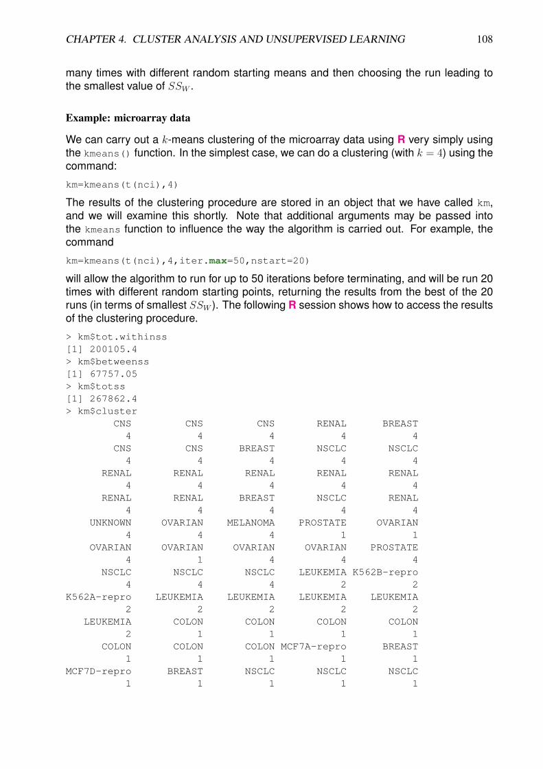
CHAPTER 4. CLUSTER ANALYSIS AND UNSUPERVISED LEARNING 108
many times with different random starting means and then choosing the run leading tothe smallest value of SSW .
Example: microarray data
We can carry out a k-means clustering of the microarray data using R very simply usingthe kmeans() function. In the simplest case, we can do a clustering (with k = 4) using thecommand:
km=kmeans(t(nci),4)
The results of the clustering procedure are stored in an object that we have called km,and we will examine this shortly. Note that additional arguments may be passed intothe kmeans function to influence the way the algorithm is carried out. For example, thecommand
km=kmeans(t(nci),4,iter.max=50,nstart=20)
will allow the algorithm to run for up to 50 iterations before terminating, and will be run 20times with different random starting points, returning the results from the best of the 20runs (in terms of smallest SSW ). The following R session shows how to access the resultsof the clustering procedure.
> km$tot.withinss[1] 200105.4> km$betweenss[1] 67757.05> km$totss[1] 267862.4> km$cluster
CNS CNS CNS RENAL BREAST4 4 4 4 4
CNS CNS BREAST NSCLC NSCLC4 4 4 4 4
RENAL RENAL RENAL RENAL RENAL4 4 4 4 4
RENAL RENAL BREAST NSCLC RENAL4 4 4 4 4
UNKNOWN OVARIAN MELANOMA PROSTATE OVARIAN4 4 4 1 1
OVARIAN OVARIAN OVARIAN OVARIAN PROSTATE4 1 4 4 4
NSCLC NSCLC NSCLC LEUKEMIA K562B-repro4 4 4 2 2
K562A-repro LEUKEMIA LEUKEMIA LEUKEMIA LEUKEMIA2 2 2 2 2
LEUKEMIA COLON COLON COLON COLON2 1 1 1 1
COLON COLON COLON MCF7A-repro BREAST1 1 1 1 1
MCF7D-repro BREAST NSCLC NSCLC NSCLC1 1 1 1 1
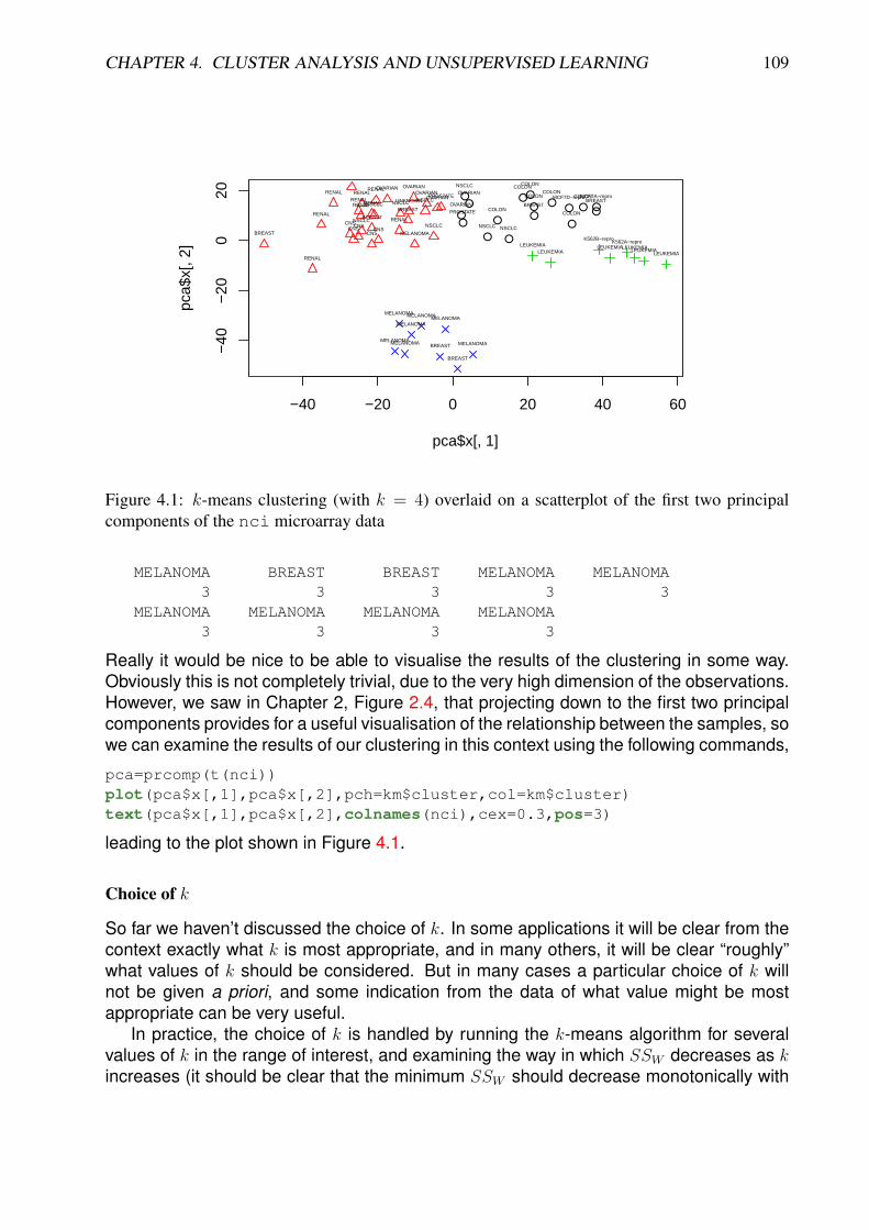
CHAPTER 4. CLUSTER ANALYSIS AND UNSUPERVISED LEARNING 109
●
●
●● ●
●●
● ●●
●●●●
●
● ●
−40 −20 0 20 40 60
−40
−20
020
pca$x[, 1]
pca$
x[, 2
]
CNSCNS
CNS
RENAL
BREASTCNS
CNSBREAST
NSCLC
NSCLC
RENAL
RENAL
RENALRENAL
RENAL RENALRENAL
BREAST
NSCLC RENAL
UNKNOWN
OVARIAN
MELANOMA
PROSTATE
OVARIANOVARIAN
OVARIAN
OVARIAN
OVARIANPROSTATENSCLC NSCLC
NSCLC
LEUKEMIAK562B−repro
K562A−reproLEUKEMIALEUKEMIA
LEUKEMIALEUKEMIALEUKEMIA
COLONCOLON
COLON
COLON
COLON COLON
COLON
MCF7A−reproBREAST
MCF7D−repro
BREAST
NSCLC
NSCLC NSCLC
MELANOMABREAST
BREAST
MELANOMA
MELANOMA
MELANOMAMELANOMA
MELANOMA
MELANOMA
Figure 4.1: k-means clustering (with k = 4) overlaid on a scatterplot of the first two principalcomponents of the nci microarray data
MELANOMA BREAST BREAST MELANOMA MELANOMA3 3 3 3 3
MELANOMA MELANOMA MELANOMA MELANOMA3 3 3 3
Really it would be nice to be able to visualise the results of the clustering in some way.Obviously this is not completely trivial, due to the very high dimension of the observations.However, we saw in Chapter 2, Figure 2.4, that projecting down to the first two principalcomponents provides for a useful visualisation of the relationship between the samples, sowe can examine the results of our clustering in this context using the following commands,
pca=prcomp(t(nci))plot(pca$x[,1],pca$x[,2],pch=km$cluster,col=km$cluster)text(pca$x[,1],pca$x[,2],colnames(nci),cex=0.3,pos=3)
leading to the plot shown in Figure 4.1.
Choice of k
So far we haven’t discussed the choice of k. In some applications it will be clear from thecontext exactly what k is most appropriate, and in many others, it will be clear “roughly”what values of k should be considered. But in many cases a particular choice of k willnot be given a priori, and some indication from the data of what value might be mostappropriate can be very useful.
In practice, the choice of k is handled by running the k-means algorithm for severalvalues of k in the range of interest, and examining the way in which SSW decreases as kincreases (it should be clear that the minimum SSW should decrease monotonically with
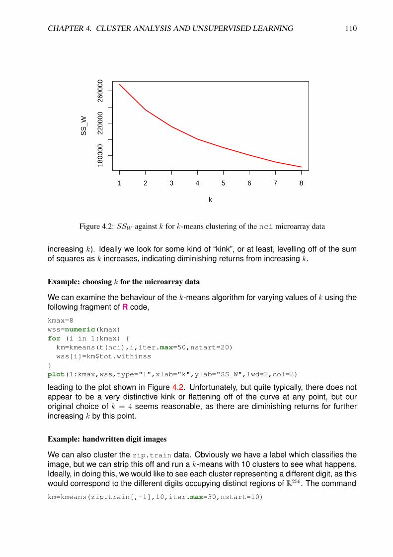
CHAPTER 4. CLUSTER ANALYSIS AND UNSUPERVISED LEARNING 110
1 2 3 4 5 6 7 8
1800
0022
0000
2600
00
k
SS
_W
Figure 4.2: SSW against k for k-means clustering of the nci microarray data
increasing k). Ideally we look for some kind of “kink”, or at least, levelling off of the sumof squares as k increases, indicating diminishing returns from increasing k.
Example: choosing k for the microarray data
We can examine the behaviour of the k-means algorithm for varying values of k using thefollowing fragment of R code,
kmax=8wss=numeric(kmax)for (i in 1:kmax) {km=kmeans(t(nci),i,iter.max=50,nstart=20)wss[i]=km$tot.withinss
}plot(1:kmax,wss,type="l",xlab="k",ylab="SS_W",lwd=2,col=2)
leading to the plot shown in Figure 4.2. Unfortunately, but quite typically, there does notappear to be a very distinctive kink or flattening off of the curve at any point, but ouroriginal choice of k = 4 seems reasonable, as there are diminishing returns for furtherincreasing k by this point.
Example: handwritten digit images
We can also cluster the zip.train data. Obviously we have a label which classifies theimage, but we can strip this off and run a k-means with 10 clusters to see what happens.Ideally, in doing this, we would like to see each cluster representing a different digit, as thiswould correspond to the different digits occupying distinct regions of R256. The command
km=kmeans(zip.train[,-1],10,iter.max=30,nstart=10)

CHAPTER 4. CLUSTER ANALYSIS AND UNSUPERVISED LEARNING 111
is quite slow to run due to the size of the data set. When it is finished we can examine thecontent of the clusters as illustrated in the following R session.
> table(zip.train[,1][km$cluster==1])
0 1 2 3 4 5 6 7 8 97 3 46 73 5 71 2 4 433 7
> table(zip.train[,1][km$cluster==2])
1 2 3 4 6 7 8 91001 3 1 42 9 3 11 5> table(Cluster=km$cluster,Digit=zip.train[,1])
DigitCluster 0 1 2 3 4 5 6 7 8 9
1 7 3 46 73 5 71 2 4 433 72 0 1001 3 1 42 0 9 3 11 53 524 0 3 2 0 15 42 0 2 04 0 0 13 2 5 3 0 445 1 615 512 0 12 1 1 7 29 0 4 06 15 0 34 546 0 296 1 0 30 27 7 0 565 12 14 9 36 2 10 08 10 0 40 8 440 40 10 23 10 1259 119 0 6 2 6 110 533 0 3 010 0 1 9 11 139 5 2 168 38 444
From the results of this analysis, we see that the cluster labelled 1 represents mainlythe digit 8, together will a few other digits, especially 3 and 5, which are fairly similar toa 8. The cluster labelled 2 mainly represents the digit 1. Cluster 3 consists mainly ofthe digit 0, but also contains a number of 6s. Note that the cluster labels are completelyarbitrary, and re-running the analysis will (hopefully) lead to similar clusters, but typicallywith a different permutation of the labels. On the basis of this very superficial analysis, itdoes appear that the digits do largely occupy different regions of R256, and so this givessome encouragement that one might be able to automatically classify digits given just theimages (we will look at classification in more detail in the next chapter).
The following code fragment shows how to look at SSW as a function of k.
kmax=15wss=numeric(kmax)for (i in 1:kmax) {print(i)km=kmeans(zip.train[,-1],i,iter.max=30,nstart=10)wss[i]=km$tot.withinss
}plot(1:kmax,wss,type="l",xlab="k",ylab="SS_W",lwd=2,col=2)
The resulting plot (not shown), perhaps surprisingly, fails to show any especially notice-able kink or flattening off at k = 10. In fact, this is just symptomatic of the general difficultyof fixing k purely on the basis of the data. More sophisticated model-based clustering pro-cedures provide principled methods for choosing k, but in most real data scenarios theevidence for one value of k over another is often very weak. See section 14.3.6 (p.509)of [HTF] for further details.
CHAPTER 4. CLUSTER ANALYSIS AND UNSUPERVISED LEARNING 112
Pre-transformation, Mahalanobis distance and the QR factorisation
Note that k-means is strongly dependent on the assumption that Euclidean distance isan appropriate metric for measuring dissimilarity of observations. If that is not the case,some kind of transformation of the data prior to clustering can be used in order to tryand ensure that Euclidean distance for the transformed data matrix is appropriate. Forexample, if Mahalanobis distance is felt to be a more appropriate metric (as it properlyaccounts for the correlation structure in the data), then the data can be standardised usinga Mahalanobis transformation prior to clustering. We have seen previously that both thesymmetric square root and Cholesky factor of the sample variance matrix can be usedto compute Mahalanobis distance, and so it will not matter if we standardise using thesymmetric square root or Cholesky factor. Further, we have shown that standardisationusing the Cholesky factor is essentially equivalent to forming the QR factorisation of thecentered data matrix. Consequently, we can cluster based on Mahalanobis distance byrunning k-means on the Q matrix of a QR factorisation. For example, we can do this forthe zip.train data as follows.
xbar=colMeans(zip.train[,-1])W=sweep(zip.train[,-1],2,xbar)QR=qr(W)km=kmeans(qr.Q(QR),10,iter.max=30,nstart=10)
Whether or not the resulting clustering will be more appropriate will be very problem de-pendent. We will come back to this issue later when we look at discrimination and classi-fication.
4.2.2 Hierarchical clustering
k-means is fast and efficient, and scales well to large data sets. However, it only makessense for observations in Euclidean space, and requires specification of the number ofclusters, k. We will now examine an approach to clustering which does not require pre-specification of the desired number of clusters, and does not require a metric distancematrix. The idea behind hierarchical clustering, often also known as agglomerative clus-tering, is to start with each observation in a separate cluster, and then join the two nearestobservations into a cluster containing just two observations. Then the algorithm proceedsat each stage by combining the clusters that are “closest” together into a new cluster.Clearly for this to make sense, we need a way of defining the distance between twoclusters, given that we know the distances between all pairs of observations. There areseveral different ways that this can be done, and each method leads to a clustering algo-rithm with different properties. However, provided that we have some way to do this, wecan describe a generic hierarchical clustering algorithm as follows.
1. Start with n clusters, C1, C2, . . . , Cn, with Ci containing just the single observation xi.The distance matrix for the n clusters is just taken to be the distance matrix for then observations.
2. Find the minimum distance, dij (if there is more than one minimum, pick one atrandom).
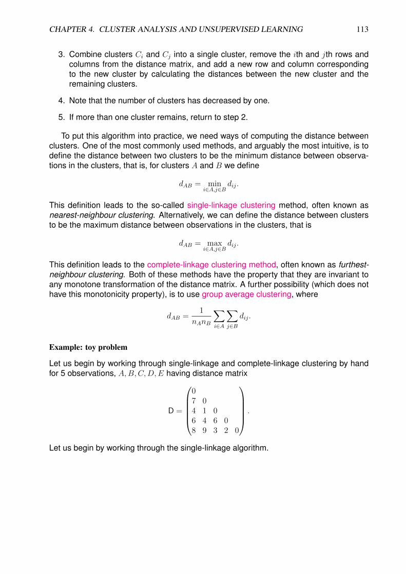
CHAPTER 4. CLUSTER ANALYSIS AND UNSUPERVISED LEARNING 113
3. Combine clusters Ci and Cj into a single cluster, remove the ith and jth rows andcolumns from the distance matrix, and add a new row and column correspondingto the new cluster by calculating the distances between the new cluster and theremaining clusters.
4. Note that the number of clusters has decreased by one.
5. If more than one cluster remains, return to step 2.
To put this algorithm into practice, we need ways of computing the distance betweenclusters. One of the most commonly used methods, and arguably the most intuitive, is todefine the distance between two clusters to be the minimum distance between observa-tions in the clusters, that is, for clusters A and B we define
dAB = mini∈A,j∈B
dij.
This definition leads to the so-called single-linkage clustering method, often known asnearest-neighbour clustering. Alternatively, we can define the distance between clustersto be the maximum distance between observations in the clusters, that is
dAB = maxi∈A,j∈B
dij.
This definition leads to the complete-linkage clustering method, often known as furthest-neighbour clustering. Both of these methods have the property that they are invariant toany monotone transformation of the distance matrix. A further possibility (which does nothave this monotonicity property), is to use group average clustering, where
dAB =1
nAnB
∑i∈A
∑j∈B
dij.
Example: toy problem
Let us begin by working through single-linkage and complete-linkage clustering by handfor 5 observations, A,B,C,D,E having distance matrix
D =
07 04 1 06 4 6 08 9 3 2 0
.
Let us begin by working through the single-linkage algorithm.
It is helpful to write out the distance matrix in the form of a

CHAPTER 4. CLUSTER ANALYSIS AND UNSUPERVISED LEARNING 114
table, asA 0
B 7 0
C 4 1 0
D 6 4 6 0
E 8 9 3 2 0
A B C D E
The minimum (off-diagonal) distance is clearly d(B,C) = 1,and so we eliminate the rows and columns for B and C, thenadd a new final row for the new cluster {B,C} as follows:
A 0
D 6 0
E 8 2 0
{B,C} 4 4 3 0
A D E {B,C}
Here the new distances have been calculated using the single-linkage minimum distance rule. Looking at the new table, wesee that the smallest off-diagonal distance is d(D,E) = 2, andso we remove D and E and add the new row {D,E} as fol-lows:
A 0
{B,C} 4 0
{D,E} 6 3 0
A {B,C} {D,E}Inspecting this new table, we see that the minimum distanceis given by d({B,C}, {D,E}) = 3, and this leads to the finaltable
A 0
{B,C,D,E} 4 0
A {B,C,D,E}

CHAPTER 4. CLUSTER ANALYSIS AND UNSUPERVISED LEARNING 115
The final step combines the remaining two clusters into a sin-gle cluster consisting of all observations.
We can display the results of a clustering process in a tree diagram known as a den-drogram by successively joining each pair of clusters in the order they were merged in theclustering algorithm, and using the vertical axis to mark the distance between the clustersat the stage they were merged. The result of this for the single-linkage clustering is shownin Figure 4.3.
We now re-do the clustering procedure using the complete-linkage method, based onmaximum distance.
We start with the distance table as previously.A 0
B 7 0
C 4 1 0
D 6 4 6 0
E 8 9 3 2 0
A B C D E
The minimum (off-diagonal) distance is clearly d(B,C) = 1,just as before, and so we eliminate the rows and columns forB and C, then add a new final row for the new cluster {B,C}as follows:
A 0
D 6 0
E 8 2 0
{B,C} 7 6 9 0
A D E {B,C}Here the new distances have been calculated using the complete-linkage maximum distance rule, and hence differ from thoseobtained previously. The minimum distance in this new tableis d(D,E) = 2, and so we merge D and E to get the new table
A 0
{B,C} 7 0
{D,E} 8 9 0
A {B,C} {D,E}
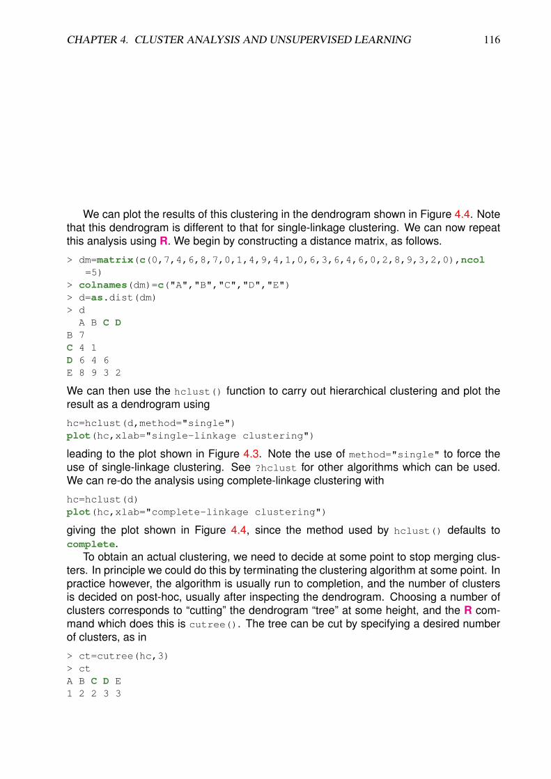
CHAPTER 4. CLUSTER ANALYSIS AND UNSUPERVISED LEARNING 116
In this new table, the minimum distance is d(A, {B,C}) = 7,and so we merge those to get
{D,E} 0
{A,B,C} 9 0
{D,E} {A,B,C}
Again, the final step is to merge the final two clusters.We can plot the results of this clustering in the dendrogram shown in Figure 4.4. Note
that this dendrogram is different to that for single-linkage clustering. We can now repeatthis analysis using R. We begin by constructing a distance matrix, as follows.
> dm=matrix(c(0,7,4,6,8,7,0,1,4,9,4,1,0,6,3,6,4,6,0,2,8,9,3,2,0),ncol=5)
> colnames(dm)=c("A","B","C","D","E")> d=as.dist(dm)> d
A B C DB 7C 4 1D 6 4 6E 8 9 3 2
We can then use the hclust() function to carry out hierarchical clustering and plot theresult as a dendrogram using
hc=hclust(d,method="single")plot(hc,xlab="single-linkage clustering")
leading to the plot shown in Figure 4.3. Note the use of method="single" to force theuse of single-linkage clustering. See ?hclust for other algorithms which can be used.We can re-do the analysis using complete-linkage clustering with
hc=hclust(d)plot(hc,xlab="complete-linkage clustering")
giving the plot shown in Figure 4.4, since the method used by hclust() defaults tocomplete.
To obtain an actual clustering, we need to decide at some point to stop merging clus-ters. In principle we could do this by terminating the clustering algorithm at some point. Inpractice however, the algorithm is usually run to completion, and the number of clustersis decided on post-hoc, usually after inspecting the dendrogram. Choosing a number ofclusters corresponds to “cutting” the dendrogram “tree” at some height, and the R com-mand which does this is cutree(). The tree can be cut by specifying a desired numberof clusters, as in
> ct=cutree(hc,3)> ctA B C D E1 2 2 3 3
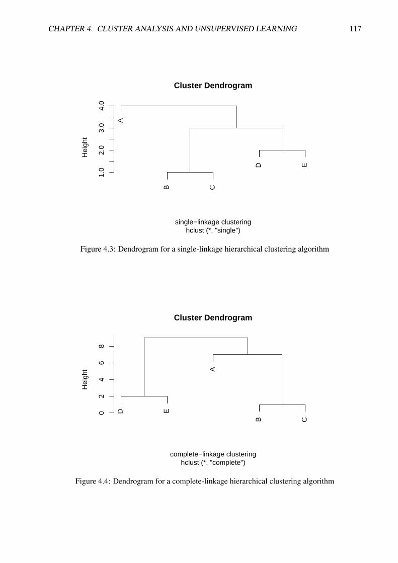
CHAPTER 4. CLUSTER ANALYSIS AND UNSUPERVISED LEARNING 117
A
B C
D E
1.0
2.0
3.0
4.0
Cluster Dendrogram
hclust (*, "single")single−linkage clustering
Hei
ght
Figure 4.3: Dendrogram for a single-linkage hierarchical clustering algorithm
D E
A
B C
02
46
8
Cluster Dendrogram
hclust (*, "complete")complete−linkage clustering
Hei
ght
Figure 4.4: Dendrogram for a complete-linkage hierarchical clustering algorithm
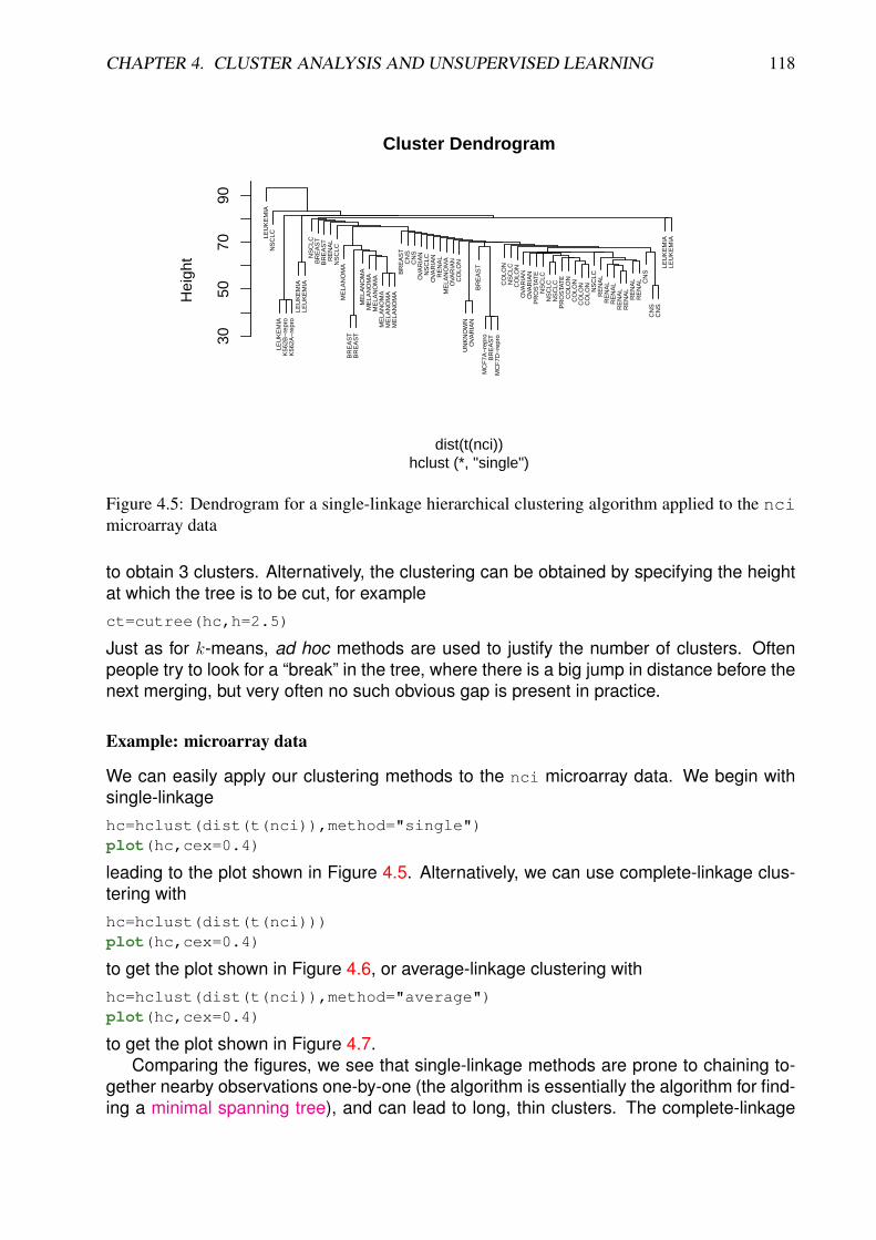
CHAPTER 4. CLUSTER ANALYSIS AND UNSUPERVISED LEARNING 118
LEU
KE
MIA
NS
CLC
LEU
KE
MIA
K56
2B−
repr
oK
562A
−re
pro
LEU
KE
MIA
LEU
KE
MIA
NS
CLC
BR
EA
ST
BR
EA
ST
RE
NA
LN
SC
LCM
ELA
NO
MA
BR
EA
ST
BR
EA
ST
ME
LAN
OM
AM
ELA
NO
MA
ME
LAN
OM
AM
ELA
NO
MA
ME
LAN
OM
AM
ELA
NO
MA
BR
EA
ST
CN
SC
NS
OV
AR
IAN
NS
CLC
OV
AR
IAN
RE
NA
LM
ELA
NO
MA
OV
AR
IAN
CO
LON
UN
KN
OW
NO
VA
RIA
NB
RE
AS
TM
CF
7A−
repr
oB
RE
AS
TM
CF
7D−
repr
oC
OLO
NN
SC
LCC
OLO
NO
VA
RIA
NO
VA
RIA
NP
RO
STA
TE
NS
CLC
NS
CLC
NS
CLC
PR
OS
TAT
EC
OLO
NC
OLO
NC
OLO
NC
OLO
NN
SC
LCR
EN
AL
RE
NA
LR
EN
AL
RE
NA
LR
EN
AL
RE
NA
LR
EN
AL CN
SC
NS
CN
SLE
UK
EM
IALE
UK
EM
IA
3050
7090
Cluster Dendrogram
hclust (*, "single")dist(t(nci))
Hei
ght
Figure 4.5: Dendrogram for a single-linkage hierarchical clustering algorithm applied to the ncimicroarray data
to obtain 3 clusters. Alternatively, the clustering can be obtained by specifying the heightat which the tree is to be cut, for examplect=cutree(hc,h=2.5)
Just as for k-means, ad hoc methods are used to justify the number of clusters. Oftenpeople try to look for a “break” in the tree, where there is a big jump in distance before thenext merging, but very often no such obvious gap is present in practice.
Example: microarray data
We can easily apply our clustering methods to the nci microarray data. We begin withsingle-linkagehc=hclust(dist(t(nci)),method="single")plot(hc,cex=0.4)
leading to the plot shown in Figure 4.5. Alternatively, we can use complete-linkage clus-tering withhc=hclust(dist(t(nci)))plot(hc,cex=0.4)
to get the plot shown in Figure 4.6, or average-linkage clustering withhc=hclust(dist(t(nci)),method="average")plot(hc,cex=0.4)
to get the plot shown in Figure 4.7.Comparing the figures, we see that single-linkage methods are prone to chaining to-
gether nearby observations one-by-one (the algorithm is essentially the algorithm for find-ing a minimal spanning tree), and can lead to long, thin clusters. The complete-linkage
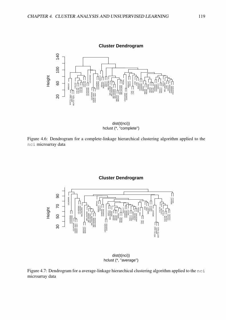
CHAPTER 4. CLUSTER ANALYSIS AND UNSUPERVISED LEARNING 119
BR
EA
ST
MC
F7A
−re
pro
BR
EA
ST
MC
F7D
−re
pro
CO
LON
CO
LON
CO
LON
CO
LON
CO
LON
CO
LON
CO
LON
LEU
KE
MIA
LEU
KE
MIA
LEU
KE
MIA
LEU
KE
MIA
K56
2B−
repr
oK
562A
−re
pro
LEU
KE
MIA
LEU
KE
MIA
NS
CLC
RE
NA
LB
RE
AS
TN
SC
LCN
SC
LCM
ELA
NO
MA
ME
LAN
OM
AM
ELA
NO
MA
ME
LAN
OM
AM
ELA
NO
MA
BR
EA
ST
BR
EA
ST
ME
LAN
OM
AM
ELA
NO
MA
RE
NA
LU
NK
NO
WN
OV
AR
IAN
BR
EA
ST
NS
CLC
CN
SC
NS
CN
SC
NS
BR
EA
ST
OV
AR
IAN
OV
AR
IAN
RE
NA
LR
EN
AL
RE
NA
L RE
NA
LR
EN
AL
RE
NA
LR
EN
AL
OV
AR
IAN
OV
AR
IAN
NS
CLC
NS
CLC
NS
CLC
NS
CLC
ME
LAN
OM
AC
NS
NS
CLC
PR
OS
TAT
EO
VA
RIA
NP
RO
STA
TE
2060
100
140
Cluster Dendrogram
hclust (*, "complete")dist(t(nci))
Hei
ght
Figure 4.6: Dendrogram for a complete-linkage hierarchical clustering algorithm applied to thenci microarray data
LEU
KE
MIA
LEU
KE
MIA
LEU
KE
MIA
LEU
KE
MIA
K56
2B−
repr
oK
562A
−re
pro
LEU
KE
MIA
LEU
KE
MIA
ME
LAN
OM
AB
RE
AS
TB
RE
AS
TM
ELA
NO
MA
ME
LAN
OM
AM
ELA
NO
MA
ME
LAN
OM
AM
ELA
NO
MA
ME
LAN
OM
AR
EN
AL
BR
EA
ST
NS
CLC
OV
AR
IAN
OV
AR
IAN
UN
KN
OW
NO
VA
RIA
NN
SC
LCM
ELA
NO
MA
RE
NA
LR
EN
AL
RE
NA
LR
EN
AL
RE
NA
LR
EN
AL
RE
NA
LN
SC
LCO
VA
RIA
NO
VA
RIA
NN
SC
LCN
SC
LCN
SC
LCP
RO
STA
TE
OV
AR
IAN
PR
OS
TAT
ER
EN
AL
CN
SC
NS
CN
SC
NS
CN
SB
RE
AS
TN
SC
LCN
SC
LCB
RE
AS
TM
CF
7A−
repr
oB
RE
AS
TM
CF
7D−
repr
oC
OLO
NC
OLO
NC
OLO
NC
OLO
NC
OLO
NC
OLO
NC
OLO
NB
RE
AS
TN
SC
LC
3050
7090
Cluster Dendrogram
hclust (*, "average")dist(t(nci))
Hei
ght
Figure 4.7: Dendrogram for a average-linkage hierarchical clustering algorithm applied to the ncimicroarray data
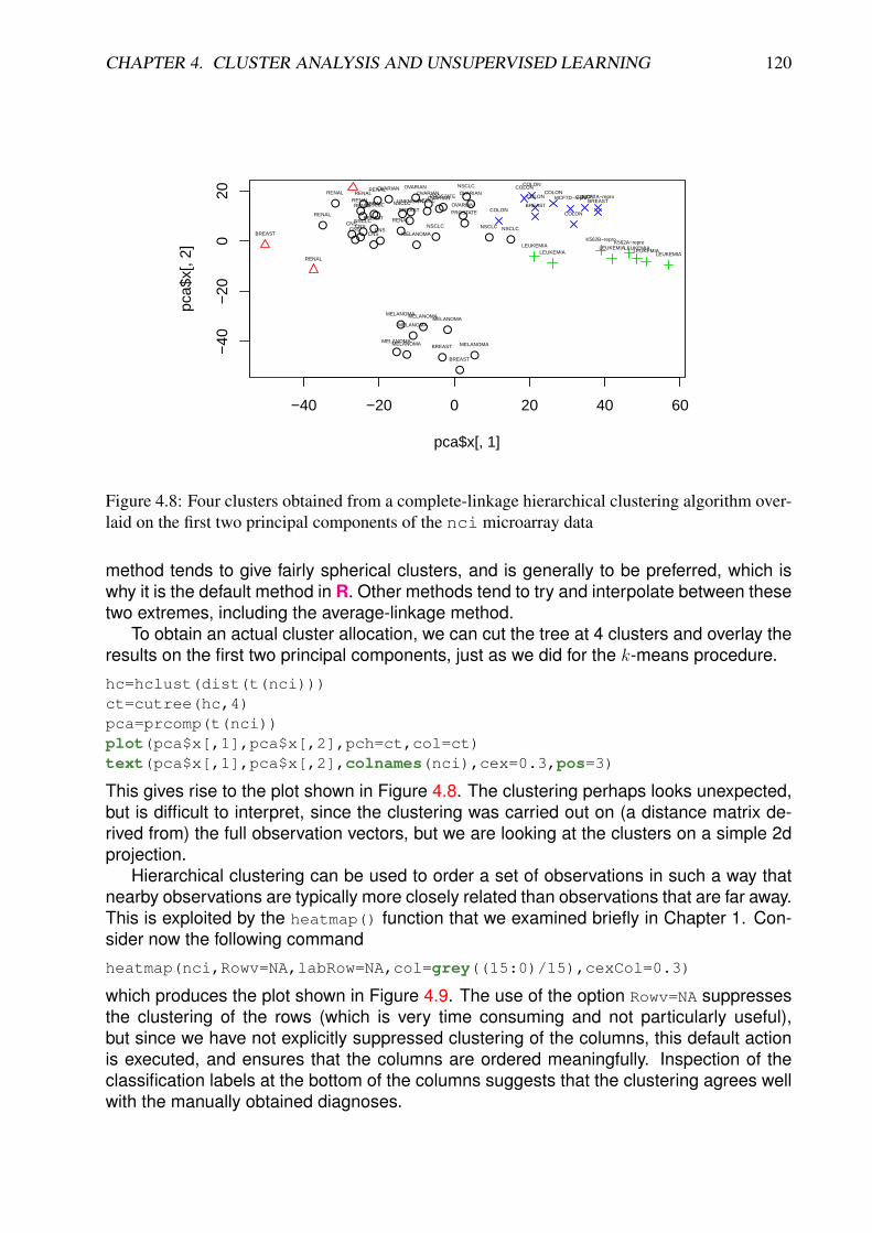
CHAPTER 4. CLUSTER ANALYSIS AND UNSUPERVISED LEARNING 120
●●●●
●●
●●●
●●● ● ●
●● ●
●
●
●
●
●●
●
●●●
● ●
●
●
● ●
●●
●
●
●
●●
●
●
−40 −20 0 20 40 60
−40
−20
020
pca$x[, 1]
pca$
x[, 2
]
CNSCNS
CNS
RENAL
BREASTCNS
CNSBREAST
NSCLC
NSCLC
RENAL
RENAL
RENALRENAL
RENAL RENALRENAL
BREAST
NSCLC RENAL
UNKNOWN
OVARIAN
MELANOMA
PROSTATE
OVARIANOVARIAN
OVARIAN
OVARIAN
OVARIANPROSTATENSCLC NSCLC
NSCLC
LEUKEMIAK562B−repro
K562A−reproLEUKEMIALEUKEMIA
LEUKEMIALEUKEMIALEUKEMIA
COLONCOLON
COLON
COLON
COLON COLON
COLON
MCF7A−reproBREAST
MCF7D−repro
BREAST
NSCLC
NSCLC NSCLC
MELANOMABREAST
BREAST
MELANOMA
MELANOMA
MELANOMAMELANOMA
MELANOMA
MELANOMA
Figure 4.8: Four clusters obtained from a complete-linkage hierarchical clustering algorithm over-laid on the first two principal components of the nci microarray data
method tends to give fairly spherical clusters, and is generally to be preferred, which iswhy it is the default method in R. Other methods tend to try and interpolate between thesetwo extremes, including the average-linkage method.
To obtain an actual cluster allocation, we can cut the tree at 4 clusters and overlay theresults on the first two principal components, just as we did for the k-means procedure.
hc=hclust(dist(t(nci)))ct=cutree(hc,4)pca=prcomp(t(nci))plot(pca$x[,1],pca$x[,2],pch=ct,col=ct)text(pca$x[,1],pca$x[,2],colnames(nci),cex=0.3,pos=3)
This gives rise to the plot shown in Figure 4.8. The clustering perhaps looks unexpected,but is difficult to interpret, since the clustering was carried out on (a distance matrix de-rived from) the full observation vectors, but we are looking at the clusters on a simple 2dprojection.
Hierarchical clustering can be used to order a set of observations in such a way thatnearby observations are typically more closely related than observations that are far away.This is exploited by the heatmap() function that we examined briefly in Chapter 1. Con-sider now the following command
heatmap(nci,Rowv=NA,labRow=NA,col=grey((15:0)/15),cexCol=0.3)
which produces the plot shown in Figure 4.9. The use of the option Rowv=NA suppressesthe clustering of the rows (which is very time consuming and not particularly useful),but since we have not explicitly suppressed clustering of the columns, this default actionis executed, and ensures that the columns are ordered meaningfully. Inspection of theclassification labels at the bottom of the columns suggests that the clustering agrees wellwith the manually obtained diagnoses.
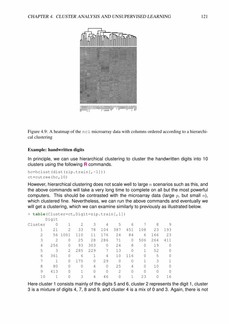
CHAPTER 4. CLUSTER ANALYSIS AND UNSUPERVISED LEARNING 121
Figure 4.9: A heatmap of the nci microarray data with columns ordered according to a hierarchi-cal clustering
Example: handwritten digits
In principle, we can use hierarchical clustering to cluster the handwritten digits into 10clusters using the following R commands.
hc=hclust(dist(zip.train[,-1]))ct=cutree(hc,10)
However, hierarchical clustering does not scale well to large n scenarios such as this, andthe above commands will take a very long time to complete on all but the most powerfulcomputers. This should be contrasted with the microarray data (large p, but small n),which clustered fine. Nevertheless, we can run the above commands and eventually wewill get a clustering, which we can examine similarly to previously as illustrated below.
> table(Cluster=ct,Digit=zip.train[,1])Digit
Cluster 0 1 2 3 4 5 6 7 8 91 21 2 33 78 104 387 451 108 23 1932 56 1001 110 11 176 24 84 6 166 233 2 0 25 28 286 71 0 506 264 4114 256 0 93 303 0 24 8 0 19 05 3 2 285 229 7 13 0 1 52 06 361 0 6 1 4 10 116 0 5 07 1 0 175 0 29 0 0 1 3 18 80 0 0 4 0 25 4 0 10 09 413 0 1 0 0 2 0 0 0 010 1 0 3 4 46 0 1 23 0 16
Here cluster 1 consists mainly of the digits 5 and 6, cluster 2 represents the digit 1, cluster3 is a mixture of digits 4, 7, 8 and 9, and cluster 4 is a mix of 0 and 3. Again, there is not
CHAPTER 4. CLUSTER ANALYSIS AND UNSUPERVISED LEARNING 122
a strong separation of digits in the clusters.See section 14.3.12 (p.520) of [HTF] for further details of hierarchical clustering meth-
ods.
4.2.3 Model-based clustering
The clustering methods we have discussed so far (k-means and hierarchical clustering)are both just heuristic data analysis techniques. However useful they are for data ex-ploration, it is difficult to use them to make strong statements about clustering in thepopulation from which they were sampled without making some modelling assumptions.The standard modelling assumption is that each cluster has a multivariate normal distri-bution, but that the different clusters have different MVN distributions. It is then possible touse maximum likelihood or Bayesian methods in order to fit these models to the availabledata. Such techniques are beyond the scope of this course, but are becoming increas-ingly widely used in modern data analysis. Such methods can be found in the CRANpackage mclust, which can be installed using install.packages("mclust") if it is notalready installed. The package can be loaded with require(mclust) and help can beobtained with ?Mclust. Note that the methods in this package typically do not scale wellto very large data sets.
In summary, we have looked in some detail at k-means clustering and at hierarchicalclustering. The advantage of k-means clustering is that it exploits the geometry of Eu-clidean space (when this makes sense), and that it scales well to very large data sets(large n). The advantages of hierarchical clustering include that it does not require a“real” metric distance matrix, and that it provides very rich information about the cluster-ing structure in the form of a dendrogram. We have not looked in detail at model-basedclustering methods, but in general these work very well (when the modelling assumptionsare reasonable), and allow much stronger inferences to be made about the populationfrom which the data is sampled, but typically do not scale well to large data scenarios(large n or large p).
Chapter 5
Discrimination and classification
5.1 Introduction
In the previous chapter we considered the rather ambitious unsupervised learning task ofautomatically grouping observations together into clusters of “similar” observations. Oftenhowever, we have some a priori idea of what kinds of groups we expect to see (or atleast, some examples of observations that have already been classified into pre-specifiedgroups), and we want to use our current understanding of the group structure in orderto automatically classify new observations which have not yet been assigned to a group.This is the statistical classification problem, and relies on partitioning the sample spaceso as to be able to discriminate between the different groups. Data that has already beenclassified into groups is often known as a training set, and methods which make use ofsuch data are often known as supervised learning algorithms.
5.2 Heuristic classifiers
5.2.1 Closest group mean classifier
Let us start by assuming that our p-dimensional observations belong to one of k groups,and that there is a mean vector associated with each group, so the group means areµ1,µ2, . . . ,µk. Now suppose that we are given an observation x ∈ Rp. Which groupshould we allocate the observation to? One obvious method would be to allocate theobservation to the group with mean that is closest to x. That is, we could allocate x togroup i if
‖x− µi‖ < ‖x− µj‖, ∀j 6= i.
This is a very simple example of a classification rule. Note that it has the effect of parti-tioning Rp into k regions, R1, R2, . . . , Rk, where Ri ⊆ Rp, i = 1, 2, . . . , k, Ri∩Rj = ∅, ∀i 6= j
and⋃ki=1Ri = Rp in such a way that x is assigned to group i if x ∈ Ri. Different classifica-
tion rules lead to different partitions, and clearly some methods of choosing the partitionwill be more effective than others for ensuring that most observations will be assigned tothe correct group. In this case, the partition is known as the Voronoi tessellation of Rp gen-erated by the “seeds” µ1,µ2, . . . ,µk. The boundaries between the classes are piecewiselinear, and to see why, we will begin by considering the case k = 2.
123

CHAPTER 5. DISCRIMINATION AND CLASSIFICATION 124
Binary classification
The case k = 2 is of particular interest, as it represents a very commonly encounteredexample in practice, and is known as binary classification. In this case one is typicallyinterested in deciding whether a particular binary variable of interest is “true” or “false”.Examples include deciding whether or not a patient has a particular disease, or decidingif a manufactured item should be flagged as potentially faulty.
In this binary case we will have 2 group means, which we can label µ1 and µ2. Underour simple classification rule we allocate x to group 1 provided that ‖x−µ1‖ < ‖x−µ2‖,otherwise we allocate to group 2. But then
‖x− µ1‖ < ‖x− µ2‖⇔ ‖x− µ1‖2 < ‖x− µ2‖2
⇔ (x− µ1)T(x− µ1) < (x− µ2)T(x− µ2)
⇔ xTx− 2µ1Tx + µ1
Tµ1 < xTx− 2µ2
Tx + µ2Tµ2
⇔ 2(µ2 − µ1)Tx < µ2Tµ2 − µ1
Tµ1
⇔ (µ2 − µ2)Tx <1
2(µ2 − µ1)T(µ2 + µ1)
⇔ (µ2 − µ1)T
[x− 1
2(µ1 + µ2)
]< 0
⇔ (µ1 − µ2)T
[x− 1
2(µ1 + µ2)
]> 0.
Note carefully how the quadratic term xTx cancels out to leave a discrimination rulethat is linear in x. If we think about the boundary between the two classes, this is clearlygiven by solutions to the equation
(µ1 − µ2)T
[x− 1
2(µ1 + µ2)
]= 0.
The first thing to note is that this boundary passes through the midpoint of the groupmeans, 1
2(µ1 + µ2), and the next thing to note is that it represents a (shifted) hyperplane∗
orthogonal to the vector µ1−µ2. That is, the boundary is the separating hyperplane whichperpendicularly bisects µ1 and µ2 at their mid-point.
For k > 2, it is clear that x will be allocated to group i if
(µi − µj)T[x− 1
2(µi + µj)
]> 0, ∀j 6= i.
∗Because of the shift, the boundary is technically an affine set and not a hyperplane, which should pass through theorigin. However, most people ignore this distinction and refer to the boundary as a hyperplane.
CHAPTER 5. DISCRIMINATION AND CLASSIFICATION 125
It is then clear that the region Ri will be an intersection of half-spaces, and hence a convexpolytope.
Example: Toy problem
To illustrate the basic idea, we will illustrate it using an example with k = 2 and p =2. Suppose that the group means are µ1 = (−1, 2)T and µ2 = (2, 1)T. What is theclassification rule?
We first compute the mid-point
1
2(µ1 + µ2) =
(0.5
1.5
),
and the difference between the means
µ1 − µ2 =
(−3
1
).
Then we allocate to group 1 if
(−3, 1)
[(x1
x2
)−(
0.5
1.5
)]> 0
⇒ −3x1 + x2 + 1.5− 1.5 > 0
⇒ x2 > 3x1.
Therefore the boundary is given by the line x2 = 3x1. Observations lying above theline will be allocated to group 1, and those falling below will be allocated to group 2.
5.2.2 Linear discriminant analysis (LDA)
The closest group mean classifier is a simple and natural way to discriminate betweengroups, and is clearly very closely related to the method of k-means clustering. However,like (basic) k-means clustering, it ignores the covariance structure in the data, includingthe fact that some variables are more variable than others. The more variable (and morehighly correlated) variables are likely to dominate the Euclidean distance, and hence willhave a disproportionate effect on the classification rule. We could correct for this by firstapplying a standardisation transformation to the data and the group means, and then carryout closest group mean classification, or we can directly adapt our rule to take covariancestructure into account. The simplest case of this arises when the k groups have differentmeans µ1,µ2, . . . ,µk, but common variance matrix Σ. In this case we can standardiseusing (say) the symmetric square root Σ−1/2, and allocate x to group i if
‖Σ−1/2x− Σ−1/2µi‖ < ‖Σ−1/2x− Σ−1/2µj‖, ∀j 6= i.
CHAPTER 5. DISCRIMINATION AND CLASSIFICATION 126
Note that we are implicitly relying on linearity of expectation here to appropriately trans-form the group means. We can write this rule differently by noting that
‖Σ−1/2x− Σ−1/2µi‖ < ‖Σ−1/2x− Σ−1/2µj‖, ∀j 6= i
⇔ ‖Σ−1/2(x− µi)‖2 < ‖Σ−1/2(x− µj)‖2, ∀j 6= i
⇔ (x− µi)TΣ−1(x− µi) < (x− µj)TΣ−1(x− µj), ∀j 6= i.
That is, we will allocate to the group whose mean is closest when measured according toMahalanobis distance. Again, this rule simplifies considerably as
(x− µi)TΣ−1(x− µi) < (x− µj)TΣ−1(x− µj)⇔ xTΣ−1x− 2µi
TΣ−1x + µiTΣ−1µi < x
TΣ−1x− 2µjTΣ−1x + µj
TΣ−1µj
⇔ 2(µj − µi)TΣ−1x < (µj − µi)TΣ−1(µj + µi)
⇔ (µj − µi)TΣ−1x− 1
2(µj − µi)TΣ−1(µj + µi) < 0
⇔ (µj − µi)TΣ−1
[x− 1
2(µi + µj)
]< 0
⇔ (µi − µj)TΣ−1
[x− 1
2(µi + µj)
]> 0.
Again note how the quadratic term, here xTΣ−1x, cancels on both sides to give a lineardiscrimination rule. Again region Ri is a convex polytope corresponding to an intersectionof half-spaces. In the binary case, the boundary between groups 1 and 2 is given by
(µ1 − µ2)TΣ−1
[x− 1
2(µ1 + µ2)
]= 0,
which again passes through the mid-point 12(µ1 + µ2), but is now the hyperplane orthog-
onal to Σ−1(µ1−µ2). This classification rule is known as Fisher’s linear discriminant, andis one of the most fundamental results in classification theory.
Example: Toy problem
Let us reconsider the toy example introduced previously, but now assume a commonvariance of
Σ =
(1 11 4
).
What is the linear discriminant in this case?
CHAPTER 5. DISCRIMINATION AND CLASSIFICATION 127
The mid-point is as before, but the normal is now given by
Σ−1(µ1 − µ2) =1
3
(4 −1
−1 1
)(−3
1
)=
1
3
(−13
4
).
Therefore we allocate to group 1 if1
3(−13, 4)
[(x1
x2
)−(
0.5
1.5
)]> 0
⇒ −13x1 + 4x2 + 0.5 > 0
⇒ x2 >13
4x1 −
1
8.
So the boundary is now given by the line x2 = 13x1/4 − 1/8, which is very similar,but different, to the boundary we computed by ignoring the variance structure. The 2boundaries, together with some simulated data, are shown in Figure 5.1.
Computational considerations
Computationally, it is often most efficient to Mahalanobis transform the data and then carryout nearest group mean classification. This can be accomplished using the Choleskyfactorisation of Σ.
Note that in the high-dimensional case, p >> k, there is an additional simplificationwhich can arise, due to the fact that the k group means must all lie in a (k−1)-dimensionalsubspace of Rp. Since the rule is to allocate to the closest group mean, all data may beprojected down to this (k−1)-dimensional space, and the classification may be carried outin Rk−1, since any components orthogonal to this subspace contribute the same distanceto each of the group means, and therefore cancel out of the classification rule. Whenk << p this dimension reduction can result in significant computational savings.
The natural basis vectors for this (k − 1)-dimensional space are known as discrimina-tion coordinates, or crimcoords, but their derivation and use is beyond the scope of thiscourse.
5.2.3 Quadratic discrimination
When the variance matrices in the groups are unequal, so that the group means areµ1, . . . ,µk and the variance matrices are Σ1, . . . ,Σk, an obvious first attempt at adaptingthe previous classification method would be to compare Mahalanobis distances for eachgroup using a distance appropriate to each group. That is, allocate observation x to groupi if
(x− µi)TΣi−1(x− µi) < (x− µj)TΣj
−1(x− µj),∀j 6= i.
Note that now the quadratic terms will not cancel, and so we end up with quadratic bound-aries. In particular, in the binary case, we will allocate x to group 1 if
(x− µ1)TΣ1
−1(x− µ1) < (x− µ2)TΣ2
−1(x− µ2),
CHAPTER 5. DISCRIMINATION AND CLASSIFICATION 128
and so the boundary between the two groups will correspond to a contour of a quadraticform.
Note that although the above approach to constructing a quadratic discrimination ruleis attractive, it does not penalise groups with large variances sufficiently. We will see laterhow to improve on this quadratic rule by attempting to take a more principled model-basedapproach.
5.2.4 Discrimination functions
We have now looked at several different methods for discrimination and classification,each leading to a different rule. However, all of the rules we have considered so far canbe described in within a common framework by introducing the concept of a discriminantfunction. For each class i = 1, 2, . . . , k, we define a corresponding function
Qi(·) : Rp −→ R,known as a discriminant function which determines a partition of Rp, R1, R2, . . . , Rk, byassigning an observation x to Ri if
Qi(x) > Qj(x), ∀j 6= i.
Note the use of a > inequality rather than a < inequality, so instead of a measure of dis-tance or dissimilarity, the discriminant functions represent the likelihood or propensity ofan observation to belong to a particular group. This turns out to be more natural and con-venient, especially in the context of model-based methods for classification. Our distance-based methods can be easily viewed within this framework by introducing a minus sign.Thus, our closest group mean classifier corresponds to the discriminant functions
Qi(x) = −‖x− µi‖2, i = 1, 2, . . . , k,
and the LDA method corresponds to
Qi(x) = −(x− µi)TΣ−1(x− µi), i = 1, 2, . . . , k.
Our first attempt at a quadratic classification rule corresponds to the discriminant func-tions,
Qi(x) = −(x− µi)TΣi−1(x− µi), i = 1, 2, . . . , k,
but as previously mentioned, we will improve on this in due course.It turns out that most classification methods of practical interest can be cast into the
framework of discriminant functions, and having a common framework can be useful inorder to develop generic techniques for the computation, interpretation and analysis ofclassification methods and procedures that are not specific to a particular discriminationtechnique.
There are many different approaches that can be taken to classification. Many, suchas those we have been considering so far, are heuristically derived. However, givena particular set of discriminant functions, we can study the properties of the resultingclassifier, such as misclassification rates, either empirically, or theoretically, to try andestablish whether the method is good or bad.
Other approaches to classification start from modelling assumptions, and derive clas-sification rules which are “optimal” in some narrowly defined sense. We will next examineone such approach, based on the assumption of multivariate normality and the principleof maximum likelihood.
CHAPTER 5. DISCRIMINATION AND CLASSIFICATION 129
5.3 Maximum likelihood discrimination
Model-based approaches to classification assume a probability model for each group, ofthe form fi(·) : Rp −→ R, i = 1, 2, . . . , k. So for observations x ∈ Rp, each model fi(x)represents a probability density function (or likelihood) for the random variable X fromgroup i. The maximum likelihood discriminant rule (MLDR) is to classify observationsby assigning them to the group with the maximum likelihood. In other words, MLDRcorresponds to using the discriminant functions
Qi(x) = fi(x), i = 1, 2, . . . , k.
5.3.1 LDA
The simplest case of maximum likelihood discrimination arises in the case where it is as-sumed that observations from all groups are multivariate normal, and all share a commonvariance matrix, Σ. That is observations from group i are assumed to be iid N(µi,Σ)random variables. In other words,
Qi(x) = fi(x) = (2π)−p/2|Σ|−1/2 exp
{−1
2(x− µi)TΣ−1(x− µi)
}.
We can simplify things by noting that
Qi(x) > Qj(x)
⇔ (2π)−p/2|Σ|−1/2 exp
{−1
2(x− µi)TΣ−1(x− µi)
}> (2π)−p/2|Σ|−1/2
× exp
{−1
2(x− µj)TΣ−1(x− µj)
}⇔ exp
{−1
2(x− µi)TΣ−1(x− µi)
}> exp
{−1
2(x− µj)TΣ−1(x− µj)
}⇔ −(x− µi)TΣ−1(x− µi) > −(x− µj)TΣ−1(x− µj),
and so the MLDR is in fact exactly equivalent to using
Qi(x) = −(x− µi)TΣ−1(x− µi).
But this is just classification by minimising Mahalanobis distance, and hence correspondsto Fisher’s linear discriminant, which allocates to group i if
(µi − µj)TΣ−1[x− 1
2(µi + µj)
]> 0, ∀j 6= i.
So in the case of equal variance matrices, the MLDR corresponds exactly to Fisher’slinear discriminant.
CHAPTER 5. DISCRIMINATION AND CLASSIFICATION 130
5.3.2 Quadratic discriminant analysis (QDA)
It is natural to next consider how the MLDR changes when we allow the variance matricesassociated with each group to be unequal. That is, we assume that observations fromgroup i are iid N(µi,Σi). In this case we have
Qi(x) = fi(x) = (2π)−p/2|Σi|−1/2 exp
{−1
2(x− µi)TΣi
−1(x− µi)}.
We can simplify this a little by noting that
Qi(x) > Qj(x)
⇔ (2π)−p/2|Σi|−1/2 exp
{−1
2(x− µi)TΣi
−1(x− µi)}> (2π)−p/2|Σj|−1/2
× exp
{−1
2(x− µj)TΣj
−1(x− µj)}
⇔ |Σi|−1/2 exp
{−1
2(x− µi)TΣi
−1(x− µi)}> |Σj|−1/2 exp
{−1
2(x− µj)TΣj
−1(x− µj)}
⇔ − log |Σi| − (x− µi)TΣi−1(x− µi) > − log |Σj| − (x− µj)TΣj
−1(x− µj),
and so the MLDR is exactly equivalent to using the discriminant function
Qi(x) = − log |Σi| − (x− µi)TΣi−1(x− µi).
Note that this is a quadratic form in x, but is different to the quadratic discriminant func-tion we derived heuristically, due to the presence of the log |Σi| term, which has the effectof appropriately penalising the distances associated with groups having large variances.This penalty term, which corresponds to the normalisation constant of the density, gen-erally improves the performance of the classifier, and hence is the form typically used inQDA.
The binary case
In the k = 2 case, we assign to group 1 if Q1(x) > Q2(x), that is
− log |Σ1| − (x− µ1)TΣ1
−1(x− µ1) > − log |Σ2| − (x− µ2)TΣ2
−1(x− µ2)
⇔ log |Σ1|+ (x− µ1)TΣ1
−1(x− µ1) < log |Σ2|+ (x− µ2)TΣ2
−1(x− µ2).
Multiplying out and gathering terms gives
xT(Σ1−1 − Σ2
−1)x+ 2(µ2TΣ2
−1 − µ1TΣ1
−1)x+ µ1TΣ1
−1µ1 − µ2TΣ2
−1µ2 + log|Σ1||Σ2|
< 0.
Here we can see explicitly that the quadratic term does not cancel out, and that the bound-ary between the two classes corresponds to the contour of a quadratic form.
CHAPTER 5. DISCRIMINATION AND CLASSIFICATION 131
5.3.3 Estimation from data
Typically the group mean vectors and variance matrices are not known in advance, butcan be estimated from data that has already been classified, typically referred to as atraining set. For the MLDR, maximum likelihood parameter estimates should be pluggedinto the discriminant functions. So, one can start with the group sample means xi andplug these in for the µi, for both LDA and QDA. The variance matrices are slightly morecomplicated. For QDA, the group sample variance matrices, Si can be plugged in for Σi.Technically, a divisor of ni rather than ni−1 should be used, since it is the MLE of variancethat is required, but it will obviously not make much difference if ni is large. However, ifΣi = (ni − 1)Si/ni is used, the discriminant function becomes
Qi(x) = − log |Σi| − (x− xi)TΣi−1(x− xi).
For LDA, a single pooled estimate of variance is required. The unbiased pooled estimateof Σ is
SW =1
n− k
k∑i=1
(ni − 1)Si,
and this can be plugged in for Σ. The corresponding MLE is
Σ =n− kn
SW ,
but note that here it doesn’t matter what divisor is used, since it will cancel out of Fisher’slinear discriminant. Also note that it is not appropriate to use the overall sample variancematrix, S, since the means within the groups are different. The discriminant functionbecomes
Qi(x) = −(x− xi)TSW−1(x− xi).
In this case, Fisher’s linear discriminant for k = 2 takes the form, allocate to group 1 if
(x1 − x2)TSW
−1{x− 1
2(x1 + x2)
}> 0.
Example: Toy problem
Now that we know how to use data in order to construct discriminant rules, we can seehow to use R to do so. We will first consider simulated data based on the simple toy modelconsidered previously. We will simulate 20 observations from each group, using the groupmeans and common variance previously given, and store the results in a 40× 2 matrix, X,and a group vector Class.
mu1=c(-1,2)mu2=c(2,1)diff=mu1-mu2ave=0.5*(mu1+mu2)Sigma=matrix(c(1,1,1,4),ncol=2)Gt=chol(Sigma)Z=matrix(rnorm(80),ncol=2)W=Z %*% Gt
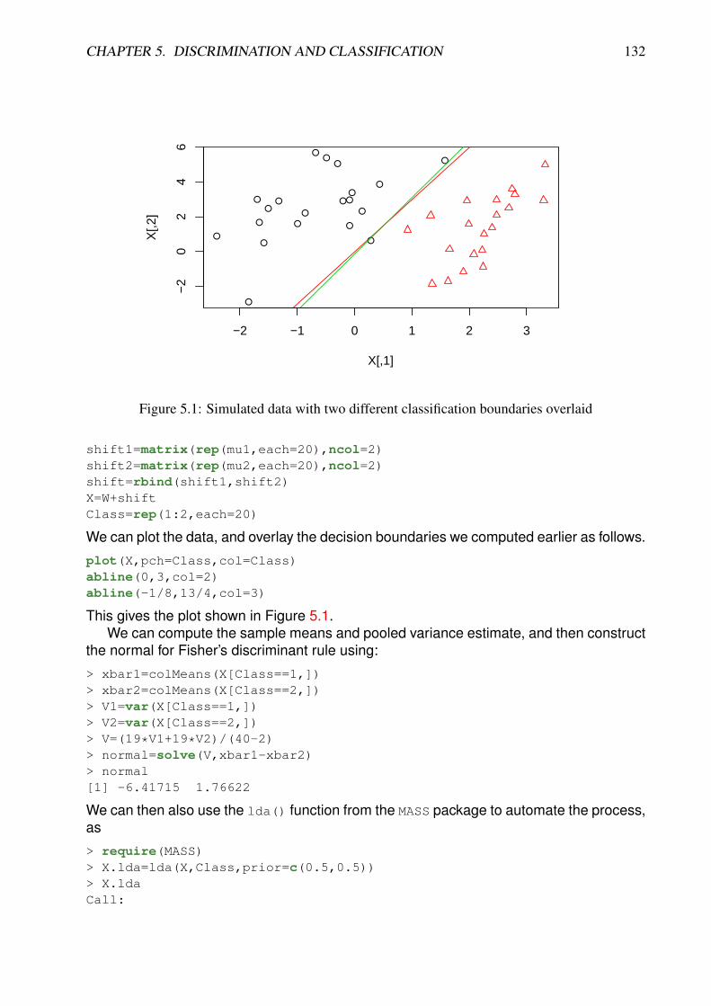
CHAPTER 5. DISCRIMINATION AND CLASSIFICATION 132
●
●
●
●
●
●
●
●●
●
●
●
●
●
●
●●
● ●
●
−2 −1 0 1 2 3
−2
02
46
X[,1]
X[,2
]
Figure 5.1: Simulated data with two different classification boundaries overlaid
shift1=matrix(rep(mu1,each=20),ncol=2)shift2=matrix(rep(mu2,each=20),ncol=2)shift=rbind(shift1,shift2)X=W+shiftClass=rep(1:2,each=20)
We can plot the data, and overlay the decision boundaries we computed earlier as follows.
plot(X,pch=Class,col=Class)abline(0,3,col=2)abline(-1/8,13/4,col=3)
This gives the plot shown in Figure 5.1.We can compute the sample means and pooled variance estimate, and then construct
the normal for Fisher’s discriminant rule using:
> xbar1=colMeans(X[Class==1,])> xbar2=colMeans(X[Class==2,])> V1=var(X[Class==1,])> V2=var(X[Class==2,])> V=(19*V1+19*V2)/(40-2)> normal=solve(V,xbar1-xbar2)> normal[1] -6.41715 1.76622
We can then also use the lda() function from the MASS package to automate the process,as
> require(MASS)> X.lda=lda(X,Class,prior=c(0.5,0.5))> X.ldaCall:
CHAPTER 5. DISCRIMINATION AND CLASSIFICATION 133
lda(X, grouping = Class, prior = c(0.5, 0.5))
Prior probabilities of groups:1 2
0.5 0.5
Group means:1 2
1 -0.6744606 2.5547252 2.1881006 1.346963
Coefficients of linear discriminants:LD1
[1,] 1.4540364[2,] -0.4002007
Setting the prior option to be uniform over the two classes ensures that we obtain theMLDR. However, leaving this option out allows the lda() function to estimate the groupfrequencies and use this in the classification rule. This turns out to be very helpful ingeneral — see the discussion about Bayesian classification at the end of the chapter.
By comparing the ratios of elements, it should be clear that the normal computed bythe lda() function is in exactly the same direction as that which we computed explicitly.The object X.lda can be passed into the predict() function in order to make actualclassifications on new data. For example, to classify the single observation x = (−3, 1),we can use predict(X.lda,c(-3,1))$class, but we can also pass in a 2-column matrixand get back a vector of classifications. For example, if we want to classify the data weused in order to build the discriminant function (in order to see how well the classifierworks), then we can do so using
> predict(X.lda,X)$class[1] 1 1 1 1 1 1 1 1 1 1 1 1 1 1 1 1 1 1 1 1 2 2 2 2 2 2 2 2 2 2 2 2 2
[34] 2 2 2 2 2 2 2Levels: 1 2
We can also use R to carry out QDA for us, using the qda() function (also from theMASS package).
X.qda=qda(X,Class)X.qda=qda(X,Class,prior=c(0.5,0.5))X.qda
The object returned from the qda() function can also be passed into the predict()function in order to classify new data.
5.4 Misclassification
Obviously, whatever discriminant functions we use, we will not characterise the groupof interest perfectly, and so some future observations will be classified incorrectly. Anobvious way to characterise a classification scheme is by some measure of the degree ofmisclassification associated with the scheme. For a fully specified model, we can define
CHAPTER 5. DISCRIMINATION AND CLASSIFICATION 134
a k × k matrix P of classification probabilities with elements
pij = P(allocate to group i|observation from group j) .
Ideally we would like this to be Ik, but in practice the best we can hope for is that thediagonal elements are close to one, and that the off-diagonal elements are close to zero.†
One way of characterising the overall quality of a classification scheme would be usingTr (P) /k, with larger values of this quality score representing better schemes, and a max-imum value of 1 indicating a perfect classification scheme.
For simple fully specified models and classification schemes, it may be possible tocompute the pij directly, analytically (see homework assignment). For models where theparameters have been estimated from data, it may be possible to estimate pij, the prob-ability obtained from the model by plugging in MLEs for the model parameters. Evenwhere this is possible, it is likely to lead to over-estimates of the diagonal elements andunder-estimates of the off-diagonal elements, due to over-fitting, and ignoring samplingvariability in the parameter estimates.
Where there is no underlying model, or the model or classification scheme is complex,it is quite likely that it will not be possible to compute P directly. In this case we can obtainempirical estimates of the pij directly from data. The plug-in method estimates the pij byre-using the data originally used to derive the classification rules. So, if we define nij tobe the number of class j observations allocated to class i (so that nj =
∑ki=1 nij), we can
estimate pij bypij =
nijnj.
That is, we estimate the probability that a class j observation is classified as class i bythe observed proportion of class j observations that are classified as class i. Althoughthis method is very simple, and very widely used, it also leads to over-optimistic estimatesof the quality of the classification scheme by testing the classifier on the data used in itsconstruction (over-fitting).
Example: Toy problem
We can create classification tables in R for the simple examples we considered earlier byusing the table() command.
> tab=table(Predicted=predict(X.lda)$class,Actual=Class)> tab
ActualPredicted 1 2
1 20 02 0 20
>> tab=table(Predicted=predict(X.qda)$class,Actual=Class)> tab
ActualPredicted 1 2
†Note that P is a left stochastic matrix, having similar properties (such as columns summing to one) as the transitionmatrix of a Markov chain.
CHAPTER 5. DISCRIMINATION AND CLASSIFICATION 135
1 20 02 0 20
A more reliable way of estimating the performance of a classifier in the case of verylarge n is to split the data set (randomly) into two, and then use one half of the dataset to train the classifier and the other half to test the performance of the classifier onindependent data.
Example: handwritten digits
We can use the data in the file zip.train in order to build a linear classifier for thehandwritten digits, and then test this classifier on the data zip.test.
> zip.lda=lda(zip.train[,-1],zip.train[,1],prior=rep(0.1,10))> tab=table(Predicted=predict(zip.lda,zip.test[,-1])$class,Actual=zip.
test[,1])> tab
ActualPredicted 0 1 2 3 4 5 6 7 8 9
0 342 0 7 3 1 4 0 0 5 01 0 251 2 0 4 0 0 1 0 02 0 0 155 3 6 0 3 0 2 03 4 2 4 142 0 17 0 2 11 04 3 5 12 3 174 3 3 7 7 45 1 0 2 9 0 125 3 0 4 06 4 3 1 0 2 0 158 0 0 07 0 0 1 1 2 0 0 129 0 58 4 1 14 4 1 6 3 1 135 39 1 2 0 1 10 5 0 7 2 165
> tab2=t(t(tab)/colSums(tab))> round(tab2,digits=2)
ActualPredicted 0 1 2 3 4 5 6 7 8 9
0 0.95 0.00 0.04 0.02 0.00 0.02 0.00 0.00 0.03 0.001 0.00 0.95 0.01 0.00 0.02 0.00 0.00 0.01 0.00 0.002 0.00 0.00 0.78 0.02 0.03 0.00 0.02 0.00 0.01 0.003 0.01 0.01 0.02 0.86 0.00 0.11 0.00 0.01 0.07 0.004 0.01 0.02 0.06 0.02 0.87 0.02 0.02 0.05 0.04 0.025 0.00 0.00 0.01 0.05 0.00 0.78 0.02 0.00 0.02 0.006 0.01 0.01 0.01 0.00 0.01 0.00 0.93 0.00 0.00 0.007 0.00 0.00 0.01 0.01 0.01 0.00 0.00 0.88 0.00 0.038 0.01 0.00 0.07 0.02 0.00 0.04 0.02 0.01 0.81 0.029 0.00 0.01 0.00 0.01 0.05 0.03 0.00 0.05 0.01 0.93
> sum(diag(tab2))/10[1] 0.8745323
We see that the classification is generally good, but ’2’s are sometimes misclassified as’4’s or ’8’s, and similarly, ’5’s are sometimes misclassified as ’3’s or ’8’s, etc.
We can repeat the analysis without requiring a uniform prior as follows.
> zip.lda=lda(zip.train[,-1],zip.train[,1])
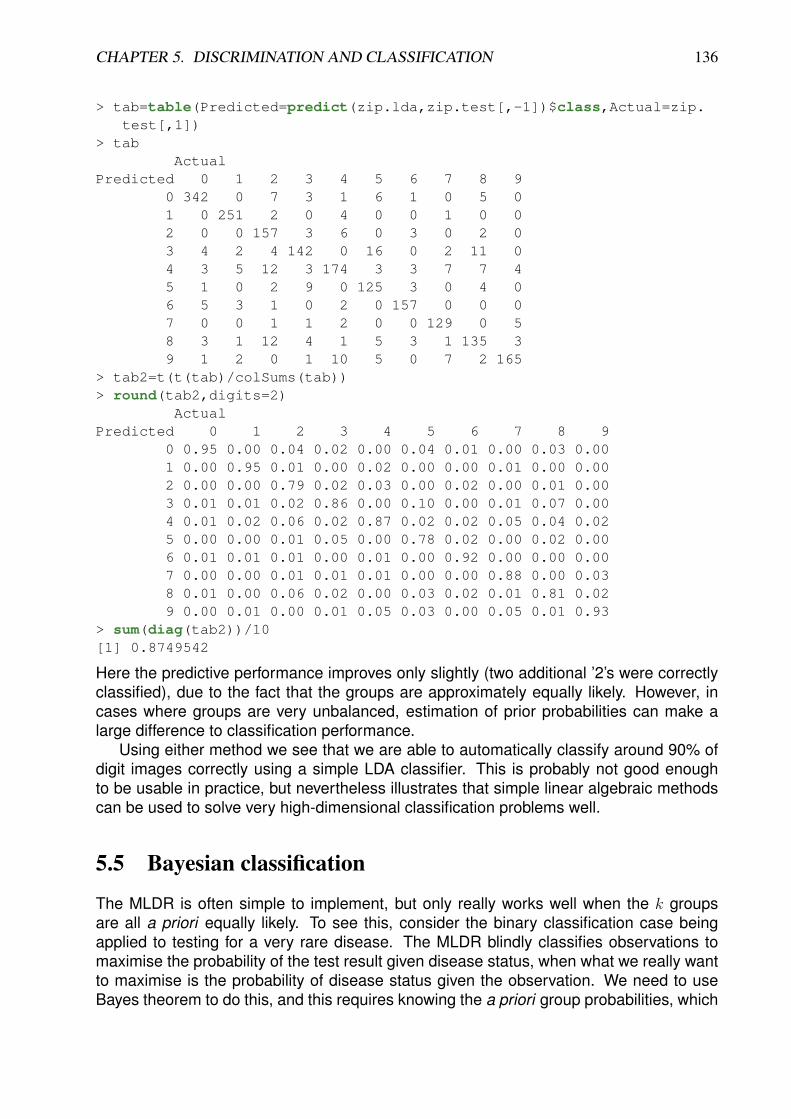
CHAPTER 5. DISCRIMINATION AND CLASSIFICATION 136
> tab=table(Predicted=predict(zip.lda,zip.test[,-1])$class,Actual=zip.test[,1])
> tabActual
Predicted 0 1 2 3 4 5 6 7 8 90 342 0 7 3 1 6 1 0 5 01 0 251 2 0 4 0 0 1 0 02 0 0 157 3 6 0 3 0 2 03 4 2 4 142 0 16 0 2 11 04 3 5 12 3 174 3 3 7 7 45 1 0 2 9 0 125 3 0 4 06 5 3 1 0 2 0 157 0 0 07 0 0 1 1 2 0 0 129 0 58 3 1 12 4 1 5 3 1 135 39 1 2 0 1 10 5 0 7 2 165
> tab2=t(t(tab)/colSums(tab))> round(tab2,digits=2)
ActualPredicted 0 1 2 3 4 5 6 7 8 9
0 0.95 0.00 0.04 0.02 0.00 0.04 0.01 0.00 0.03 0.001 0.00 0.95 0.01 0.00 0.02 0.00 0.00 0.01 0.00 0.002 0.00 0.00 0.79 0.02 0.03 0.00 0.02 0.00 0.01 0.003 0.01 0.01 0.02 0.86 0.00 0.10 0.00 0.01 0.07 0.004 0.01 0.02 0.06 0.02 0.87 0.02 0.02 0.05 0.04 0.025 0.00 0.00 0.01 0.05 0.00 0.78 0.02 0.00 0.02 0.006 0.01 0.01 0.01 0.00 0.01 0.00 0.92 0.00 0.00 0.007 0.00 0.00 0.01 0.01 0.01 0.00 0.00 0.88 0.00 0.038 0.01 0.00 0.06 0.02 0.00 0.03 0.02 0.01 0.81 0.029 0.00 0.01 0.00 0.01 0.05 0.03 0.00 0.05 0.01 0.93
> sum(diag(tab2))/10[1] 0.8749542
Here the predictive performance improves only slightly (two additional ’2’s were correctlyclassified), due to the fact that the groups are approximately equally likely. However, incases where groups are very unbalanced, estimation of prior probabilities can make alarge difference to classification performance.
Using either method we see that we are able to automatically classify around 90% ofdigit images correctly using a simple LDA classifier. This is probably not good enoughto be usable in practice, but nevertheless illustrates that simple linear algebraic methodscan be used to solve very high-dimensional classification problems well.
5.5 Bayesian classification
The MLDR is often simple to implement, but only really works well when the k groupsare all a priori equally likely. To see this, consider the binary classification case beingapplied to testing for a very rare disease. The MLDR blindly classifies observations tomaximise the probability of the test result given disease status, when what we really wantto maximise is the probability of disease status given the observation. We need to useBayes theorem to do this, and this requires knowing the a priori group probabilities, which

CHAPTER 5. DISCRIMINATION AND CLASSIFICATION 137
can also be estimated from data. This has the effect of introducing additional terms intothe discriminant functions. Bayesian classifies typically perform much better than heuristicmethods, or methods based on MLDR, but are beyond the scope of this course.
See section 4.3 (p.106) of [HTF] for further information about techniques for classifi-cation.
Chapter 6
Graphical modelling
6.1 Introduction
Variables of multivariate distributions and data sets are often correlated in complex ways.It would be convenient if many variables were independent, leading to a sparse indepen-dence structure, as this would lead to many simplifications of much multivariate theoryand methodology. Unfortunately variables tend not to be independent in practice. It ismore often the case that variables are conditionally independent. Although not quite asstrong a property as independence, this too turns out to be enough to lead to consider-able simplification of a general dependence structure, and is useful for both conceptualand theoretical understanding, and also for computational efficiency. Sparse conditionalindependence structures can be represented using graphs, and this leads to the theoryof graphical models. But before we explore graphical models, we must first ensure thatwe understand the notion of conditional independence.
6.2 Independence, conditional independence and factorisation
Let us begin by reminding ourselves of the essential notion of independence of eventsand random variables. For events A and B, we say that A and B are independent, andwrite A ⊥ B, if
P(A ∩B) = P(A) P(B) .
Note that for P(B) > 0 we get
P(A|B) =P(A ∩B)
P(B)= P(A) ,
which captures the intuitive notion of independence, that learning the outcome ofB shouldnot affect the probability of A.
The notion extends straightforwardly to (continuous) random quantities, where nowwe say that variables X and Y are independent and write X ⊥ Y if their joint densityfactorises as
fX,Y (x, y) = fX(x)fY (y).
Again, for fY (y) > 0 we have
fX|Y (x|y) =fX,Y (x, y)
fY (y)= fX(x),
138
CHAPTER 6. GRAPHICAL MODELLING 139
capturing the intuitive notion that the conditional distribution of X given Y = y should notdepend on y. That is, the conditional and marginal distributions should be the same.
It turns out that independence is a special case of the more general notion of con-ditional independence. For events A, B and C, we say that A and B are conditionallyindependent given C, and write A⊥⊥B|C, if
P(A ∩B|C) = P(A|C) P(B|C) .
Now, when P(B|C) > 0 we have
P(A|B ∩ C) =P(A ∩B|C)
P(B|C)= P(A|C) ,
and so conditional on C, learning the outcome of B does not change the probability of A.This notion again generalises easily to (continuous) random quantities, so that for
random variables X, Y and Z, we have that X and Y are conditionally independent givenZ, written X⊥⊥Y |Z if the conditional density of X and Y given Z = z factorises as
fX,Y |Z(x, y|z) = fX|Z(x|z)fY |Z(y|z).
So then if fY |Z > 0 we have
fX|Y,Z(x|y, z) =fX,Y |Z(x, y|z)
fY |Z(y|z)= fX|Z(x|z).
There are numerous other important properties of this factorisation for the joint density ofX, Y and Z, fX,Y,Z(x, y, z).
Proposition 31 If X⊥⊥Y |Z then the joint density factorises as
fX,Y,Z(x, y, z) = fZ(z)fX|Z(x|z)fY |Z(y|z).
This factorisation property turns out to be key to understanding directed acyclic graph(DAG) models.Proof
fX,Y,Z(x, y, z) = fZ(z)fX,Y |Z(x, y|z) = fZ(z)fX|Z(x|z)fY |Z(y|z).
�
Proposition 32 If X⊥⊥Y |Z and fZ(z) > 0, then the joint density factorises as
fX,Y,Z(x, y, z) =fX,Z(x, z)fY,Z(y, z)
fZ(z).

CHAPTER 6. GRAPHICAL MODELLING 140
This factorisation property turns out to be important for understanding undirected graphi-cal models.Proof
fX,Y,Z = fZ(z)fX|Z(x|z)fY |Z(y|z)
= fZ(z)fX,Z(x, z)
fZ(z)
fY,Z(y, z)
fZ(z)
=fX,Z(x, z)fY,Z(y, z)
fZ(z).
�
Proposition 33 Assuming that fZ(z) > 0, we have that X⊥⊥Y |Z if and only if the jointdensity factorises in the form
fX,Y,Z(x, y, z) = h(x, z)k(y, z),
for some bivariate functions h(·, ·) and k(·, ·).
ProofFirst note that the forward implication follows from Proposition 32. That is, if X⊥⊥Y |Z,
then there exist functions h(·, ·) and k(·, ·) such that
fX,Y,Z(x, y, z) = h(x, z)k(y, z).
For example, we could choose h(x, z) = fX,Z(x, z) and k(y, z) = fY,Z(y, z)/fZ(z), but thereare obviously many other possibilities.
The reverse direction is less clear. We assume that we have the factorisation
fX,Y,Z(x, y, z) = h(x, z)k(y, z),
and want to prove thatfX,Y |Z(x, y|z) = fX|Z(x|z)fY |Z(y|z).
This can be demonstrated with straightforward algebraic manipulation, but is left as anexercise. �
Note that although we may have been thinking about univariate random quantities X,Y and Z, nothing we have discussed is specific to the univariate case, and all appliessimilarly to the case of multivariate random quantities X, Y and Z.
The above factorisation results are very powerful, and can be used to prove a numberof general algebraic properties associated with independence and conditional indepen-dence of random quantities.

CHAPTER 6. GRAPHICAL MODELLING 141
Proposition 34
1. X⊥⊥Y |Z ⇔ Y⊥⊥X|Z
2. X⊥⊥Y |Z ⇒ h(X)⊥⊥Y |Z
3. X⊥⊥Y |Z ⇒ X⊥⊥Y |(Z, h(X))
4. X⊥⊥Y |Z and X⊥⊥W |(Y, Z)⇔ X⊥⊥(W,Y )|Z
5. If all densities are positive, then
X⊥⊥Y |Z and X⊥⊥Z|Y ⇒ X ⊥ (Y, Z).
ProofThe proofs of these results are mainly straightforward, and left as an exercise. �
6.3 Undirected graphs
6.3.1 Graph theory
It turns out that when we have a large number of variables with many associated condi-tional independence statements, it is useful to represent known statements using a graph.The graphs used can be directed or undirected, and can be given several different inter-pretations. We begin with a reminder of some basic properties of undirected graphs, andthen later examine how such graphs may be associated with conditional independenceproperties.
A graph G is a tuple G = (V,E), where V = {v1, v2, . . . , vn} is a finite set of vertices (ornodes), and E is a finite set of undirected edges, with each edge e ∈ E being of the forme = {vi, vj}, vi, vj ∈ V , i 6= j. There are clearly
(n2
)= n(n − 1)/2 possible edges of this
form, and we write(V2
)for the set of all such edges, so that E ⊆
(V2
). A graph is said to
be complete if E =(V2
).
Example
Consider the graph G = (V,E) where V = {A,B,C} and E = {{A,C}, {B,C}}. We candraw a pictorial representation of the graph as given in Figure 6.1. Note that this graph isnot complete, since the edge {A,B} is missing. Also note that we can plot this graph inR using the ggm package, using the following commands
require(ggm)drawGraph(UG(∼ A*C+B*C))
Note that the drawGraph() function allows moving nodes around using a very simplepoint-and-click interface. The command plotGraph() can also be used, and has a moresophisticated interface, but may not be available on all systems.

CHAPTER 6. GRAPHICAL MODELLING 142
●
●
●A
C
B
Figure 6.1: A graph with 3 vertices and 2 edges
Vertices vi, vj ∈ V are said to be adjacent, written vi ∼ vj, if {vi, vj} ∈ E. Any subsetof vertices U ⊆ V induces a subgraph GU = (U, F ), where
F = {{u, v} ∈ E|u, v ∈ U}.
Example
For the graph considered in the previous example, nodes A and C are adjacent (A ∼ C),but nodes A and B are not. Similarly, the subgraph G{A,C} is complete, but the subgraphG{A,B} is not.
A subset U ⊆ V is a (maximal) clique if it is maximally complete. That is, the associ-ated subgraph GU is complete, and for all strict supersets of U , W (so that U ⊂ W ⊆ V ),the induced subgraph GW is not complete.
Example
Again, considering again the previous example, the graph G has two cliques, {A,C} and{B,C}.
Example
The previous example is somewhat uninteresting in that the cliques correspond withedges. So consider now the graph G = (V,E) where V = {D,E, F,G} and
E = {{D,E}, {D,F}, {E,F}, {E,G}}.
Draw the graph and write down the cliques. How many cliques are there?

CHAPTER 6. GRAPHICAL MODELLING 143
●
●
● ●
●
V
W
X Y
Z
Figure 6.2: A graph with 5 vertices and 3 cliques
The cliques are {D,E, F} and {E,G}. There are two cliques.Note that the set of cliques defines the graph. That is, complete knowledge of all
cliques of the graph allows construction of the graph.
Example
Consider the graph G which has three cliques: {V,W,X}, {W,X, Y } and {W,X,Z}. Wecan construct and plot this graph in R using
drawGraph(UG(∼ V*W*X+W*X*Y+W*Y*Z))
leading to the plot shown in Figure 6.2.
The neighbours of a node v ∈ V , often known as the boundary of v, written bd(v),is {u ∈ V |u ∼ v}. The closure of v, written cl(v), is given by cl(v) = v ∪ bd(v). Apath is a sequence x0, x1, . . . , xm ∈ V such that xi−1 ∼ xi, i = 1, 2, . . . ,m. A graphis connected if there exists a path between every pair of vertices. A component is amaximal connected subgraph. A cycle is a (non-trivial) path starting and ending at thesame vertex. A connected graph is a tree if it does not contain any cycles. A leaf is anynode of a tree connected to just one edge. A forest is a graph with components which areall trees.
For any undirected graph G = (V,E) with vertex subsets A,B,C ⊆ V , we say that Cseparates A and B if all paths from a node in A to a node in B pass through a node in C.
6.3.2 Graphical models
Now, given a collection of conditional independence statements relating to a collection ofrandom variables, we can define a graph by associating nodes with variables, and using
CHAPTER 6. GRAPHICAL MODELLING 144
the edge structure to encode the conditional independence structure. This is useful forboth visualisation and computational analysis. It turns out that there are several differentways that we can do this, but they all turn out to be equivalent in practice in most cases.
Given a set of random variables X1, X2, . . . , Xn, we can define an associated graphG = (V,E), where V = {X1, X2, . . . , Xn}, and E is a set of edges.
Definition 10 We say that G has the factorisation property (F) if the joint density of therandom variables factorises in the form
fX(x) =∏c∈C
φc(xc),
for some functions φc(·), where C denotes the set of cliques associated with the graph G.
Definition 11 We say that G has the global Markov property (G) if for any disjoint vertexsubsets A, B and C such that C separates A and B in G we have A⊥⊥B|C.
Definition 12 We say that G has the local Markov property (L) if for all v ∈ V we have
v⊥⊥V \ cl(v)|bd(v).
Definition 13 We say that G has the pairwise Markov property (P) if for all u, v ∈ V suchthat u 6∼ v we have
u⊥⊥v|V \{u, v}.
We have just presented four different ways that one can associate a graph with a con-ditional independence structure of a set of random variables. If these different interpreta-tions all turn out to be fundamentally different, this is potentially confusing. Fortunately, itturns out that these different interpretations are all closely linked.
Proposition 35 (F)⇒ (G)⇒ (L)⇒ (P)
This important result tells us that if a graph satisfies the factorisation property (F), thenthe other properties all follow.Proof
Let’s start with the simplest result, (G) ⇒ (L): This is trivial, since by definition, bd(v)separates v from V \ cl(v).
Now let us consider (L)⇒ (P):
Suppose (L), so that we know
v⊥⊥V \ cl(v)|bd(v).
Now using property 3 of Proposition 34, we can “copy” ver-tices from V \ cl(v) to the conditioning set as desired in orderto deduce that
v⊥⊥V \ cl(v)|V \{u, v}.
CHAPTER 6. GRAPHICAL MODELLING 145
Finally, since u and v are not adjacent, we know that u ∈V \ cl(v), and so using property 2 of Proposition 34, we con-clude that
v⊥⊥u|V \{u, v},and (P) is satisfied.
Finally, let us consider (F) ⇒ (G): Assume (F), and suppose that A, B and C aredisjoint subsets of V with C separating A and B. The graph GV \C can’t be connected, solet A be the components of GV \C containing vertices in A, so that A ⊆ A and B ∩ A = ∅due to the separation assumption. Now put B = V \(A ∪ C) so that B ⊆ B, and V is thedisjoint union of A, B and C. Again, due to the separation assumption, every c ∈ C mustbe such that c ⊆ A ∪ C or c ⊆ B ∪ C. Call the set of all cliques in A ∪ C, CA, and the restCB. Using (F), we have
f(x) =∏c∈C
φc(x) =∏c∈CA
φc(x)∏c∈CB
φc(x) = h(xA∪C)k(xB∪C),
and so A⊥⊥B|C. Now using property 2 of Proposition 34 we conclude first that A⊥⊥B|C,since A ⊆ A and then that A⊥⊥B|C, since B ⊆ B. That is, (G) is satisfied. �
Proposition 36 (Hammersley-Clifford) If all densities are positive, then (P)⇒ (F).
This important (and difficult) result is stated without proof. However, the implication is thatin most practical cases, all four interpretations of a graph of conditional independencestructures are equivalent, and may be considered interchangeably.
Corollary 1 If all densities are positive, then (F)⇔ (G)⇔ (L)⇔ (P).
6.4 Gaussian graphical models (GGMs)
We now turn attention to the simplest parametrised class of graphical models — Gaus-sian graphical models (GGMs). These are simply multivariate normal distributions wherethe variables are subject to conditional independence properties. It turns out to be verystraightforward to characterise GGMs in terms of the pairwise Markov property (P), but tounderstand why, we must first understand a little more about the MVN, and its parametri-sation in terms of the precision matrix. If X is a random vector with variance matrixVar(X), then Q = Var(X) −1 is the precision matrix for X. So, if X ∼ N(µ,Σ), we canput Q = Σ−1, and then X ∼ N(µ,Q−1). Note that we can express the density of the MVNin terms of µ and Q as
f(x) = (2π)−p/2|Q|1/2 exp
{−1
2(x− µ)TQ(x− µ)
}.
Writing the density in this way allows us to partition x, µ and Q, and derive the conditionaldistribution of the first part of x given the rest.

CHAPTER 6. GRAPHICAL MODELLING 146
Proposition 37 For X ∼ N(µ,Q−1), partition
X =
(X1
X2
), x =
(x1
x2
), µ =
(µ1
µ2
), Q =
(Q11 Q12
Q21 Q22
).
Then(X1|X2 = x2) ∼ N(µ1|2,Q11
−1),
whereµ1|2 = µ1 − Q11
−1Q12(x2 − µ2).
Proof
f (x1|x2) ∝ f (x)
∝ exp
{−1
2(x− µ)TQ(x− µ)
}∝ exp
{−1
2
[(x1 − µ1)TQ11(x1 − µ1)+
+ (x2 − µ2)TQ22(x2 − µ2)
+2(x1 − µ1)TQ12(x2 − µ2)] }
∝ exp
{−1
2
[x1
TQ11x1 − 2x1TQ11µ1 + 2x1
TQ12(x2 − µ2)]}
∝ exp
{−1
2
[x1
TQ11x1 − 2x1TQ11µ1|2
]}∝ exp
{−1
2
[(x1 − µ1|2)TQ11(x1 − µ1|2)
]}.
�
Using this result, it is straightforward to see why zeroes of Q correspond to pairwise con-ditional independence statements.
CHAPTER 6. GRAPHICAL MODELLING 147
First consider the case q12 = 0 (= q21). This is wlog, since we can always re-order thevariables to ensure that the zero of interest is in this position.∗ Partition X as
X =
(X1
X2
), where X1 =
(X1
X2
)and X2 =
X3
X4...Xp
.
Then X1|X2 = x2 has variance Q11−1, which must be diagonal, since Q11 is. Now this
means that X1 and X2 are conditionally uncorrelated, but for the MVN, uncorrelated andindependent are equivalent. Consequently X1⊥⊥X2|(X3, . . . , Xp), and so q12 = 0 leadsdirectly to this CI statement. In general, we have the following result.
Proposition 38 If X ∼ N(µ,Q−1), then for i 6= j we have
qij = 0 (= qji)⇔ Xi⊥⊥Xj|X\{Xi, Xj}.
Therefore, there is a direct correspondence between the zero structure of Q and an undi-rected graph with the pairwise Markov property (P), where zeroes in Q correspond tomissing edges in the graph. Further, provided that Q (or equivalently, the variance matrix,Σ) is strictly positive definite, the densities are all positive, and we can conclude that all ofour properties (F), (G), (L) and (P) are satisfied by the associated graph.
6.4.1 Partial covariance and correlation
We have shown that the MVN has the important and interesting property that Var(X1|X2 = x2)does not depend on the observed value of x2. This allows us to consider the conditionalvariance matrix without reference to the observed values of the variables we are condition-ing on. We define the partial (co)variance matrix for X1 (given X2) to be the conditionalcovariance matrix Q11
−1. In particular, in the case X1 = (X1, X2)T, we have
Q11−1 =
(q11 q12q12 q22
)−1=
1
q11q22 − q212
(q22 −q12−q12 q11
),
and so we define the partial covariance between X1 and X2 to be −q12/(q11q22− q212). Thecorresponding partial correlation is therefore given by −q12/
√q11q22. In general, the partial
correlation between Xi and Xj, for i 6= j is given by−qij√qiiqjj
.
Consequently, we can define the partial correlation matrix to be the matrix of partial cor-relations, and this is clearly given by
PCorr(X) = 2 Ip−D−1/2QD−1/2, where D = diag {q11, . . . , qpp} .
Note that in the typical case of positive definite Q, the zeroes of Q match those of PCorr(X).Consequently, we can understand the CI structure of a GGM by studying the zero struc-ture of the partial correlation matrix.∗Note that if P is a permutation matrix, then P is orthogonal. Then Var(PX) = PVar(X)PT, and so
Var(PX)−1 = PVar(X)−1PT, as can be verified by direct multiplication. In other words, the precision matrixfor the re-ordered variables is just the precision matrix for the variables in their original order, but with rows andcolumns re-ordered to match.

CHAPTER 6. GRAPHICAL MODELLING 148
Example: toy problem
Suppose that X = (X1, X2, X3)T ∼ N(0,Σ), where
Σ =
3 −2 1−2 4 −21 −2 3
.
Are there any conditional independence relations between the variables?
We can use R to answer this question. Note that as there are no zeroes in the variancematrix, Σ, there are no marginal independence relations between the variables. To look forconditional independence relations, we can compute the corresponding partial correlationmatrix. We could do this by hand, by first using Gaussian elimination to compute theprecision matrix, but it will be easier to use R.> Sigma=matrix(c(3,-2,1,-2,4,-2,1,-2,3),ncol=3)> Q=solve(Sigma)> Q
[,1] [,2] [,3][1,] 0.50 0.25 0.00[2,] 0.25 0.50 0.25[3,] 0.00 0.25 0.50> 2*diag(3)-diag(diag(Q)ˆ(-0.5))%*%Q%*%diag(diag(Q)ˆ(-0.5))
[,1] [,2] [,3][1,] 1.0 -0.5 0.0[2,] -0.5 1.0 -0.5[3,] 0.0 -0.5 1.0
Note that the ggm package includes the command parcor() for computing the partialcorrelation matrix directly from a variance matrix:> parcor(Sigma)
[,1] [,2] [,3][1,] 1.0 -0.5 0.0[2,] -0.5 1.0 -0.5[3,] 0.0 -0.5 1.0
which is much easier. We now see that the partial correlation in position (1,3) and (3,1)is zero, and this implies the pairwise Markov property, X1⊥⊥X3|X2. Thus, the associatedundirected graph will be a chain with X2 separating X1 and X3.
This also gives us a potential strategy for estimating a GGM from data: computethe sample partial correlation matrix for the data set, and then use the zero structureof this estimated matrix in order to identify missing edges in the GGM. Now, following thisprocedure directly will typically lead to very dense graphs, since sample estimates of zeropartial correlations will often be small, but not exactly zero. In this case we can apply athreshold to the sample partial correlation matrix, or attempt to apply statistical tests forwhether or not particular elements are significantly different from zero.
Example: Mathematics students exam marks
The ggm package includes a very famous (old!) data set on exam marks of mathematicsstudents in 5 subject areas. It can be loaded and plotted with
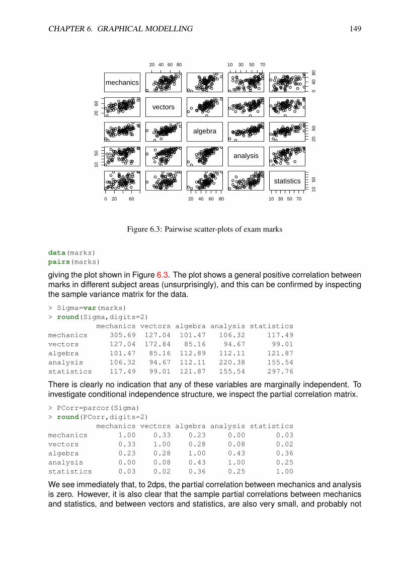
CHAPTER 6. GRAPHICAL MODELLING 149
mechanics
20 40 60 80
●●
●
●●
● ●●● ●
●●●●
●
●
●●
●
●●●
●
●●●●
●
●● ●
●●● ●
●●● ●●
●
●●● ●●
●
●●
●
●●
●●
●●● ●●●
●●
●
●
●
●
●●●
●●
●
●
●
●
●
●●
●●
● ●●●
●●
● ●
●●
●
●●
●●●●●
●●●●
●
●
● ●
●
●● ●
●
● ●●●
●
●●●
●●●●
●●●●●
●
●●●●●
●
●●●
●●
●●
●●● ●● ●
●●
●
●
●
●
●●
●
●●
●
●
●
●
●
●●
●●
●●●●●
●● ●
10 30 50 70
●●
●
●●
●●●●●●●●
●
●
●
●●
●
●●●
●
●● ●●
●
●●●
●●●●
●● ●● ●
●
●●●● ●●
●●
●
●●
●●
●● ●●●●
●●
●
●
●
●
●●
●
●●
●
●
●
●
●
●●
●●
●●● ●
●●
●● 040
80●●●
●●
●●● ●●
●● ●●
●
●
●●
●
●● ●
●
● ●●●
●
●●●
● ●●●
●● ●●●
●
●● ●●●
●
●●●
●●
●●
● ●●● ●●
●●
●
●
●
●
●●
●
●●
●
●
●
●
●
●●
●●
●●●●●●●●
2060
●● ●●●●
● ●●●
●●
●●
●●●●
●●●
●
● ●●●●
●●
●
●
●
●
●
●
●
●●
●●●●
●●●●●
● ● ●●● ●●
●●
●●●● ●
●●●
●
●●
●●
●●
●●●
● ●
●● ●
●
●
●●●
● ●●● vectors
● ●●●● ●●●
●●●●
●●●
●● ●
●●●
●
●● ●● ●●
●●
●
●
●
●
●
●
●●
●● ●●
●●
●●●
●●●● ●●●●●
●●● ●●
● ●●
●
●●
● ●
●●
●●●
●●
●●●
●
●
●●●●●●
●
●●●●●●
●●●●●●
●●●
●●●
● ●●
●
●●● ●●●
●●
●
●
●
●
●
●
●●
● ●●
●
●●
● ●●
●●● ●●●●
●●
●●●●●
●●●
●
●●
● ●
●●
●● ●
●●
●● ●
●
●
●● ●
●●●●
●●●●● ●
●●●
●●●
●●
●● ●●
● ●●
●
●● ●●●●
●●
●
●
●
●
●
●
●●
●●●
●
●●●●
●●●●● ●●
●●
●●
● ●●●●●
●
●
●●
●●
●●
●●●
●●
●●●
●
●
●●●●●●
●
●
●●
● ●●
● ●●●●●●●● ●●
● ●●●
●●●
●●
●●
●
●● ●●●● ●●●●●
●●●●
●●●
●● ●●
●● ●●●
●
●
●●
●●●
●●
●●
●
● ● ●●
●●●
●●
●●
●●
● ●●●●
●●
●
●●●●
●●●
● ●●●●●● ●●
●●●●
● ●●
●●●●
●
● ●●●● ●● ●● ●●
●● ●●
●●●
●●●●
●●● ●●
●
●
●●
●●●
●●
●●
●
●● ●●
●●●●
●
●●
●●
●●●●●
●●
algebra●
●●
●●●●●
●●●●●●●●●●● ●
●● ●
●●
●●●
●
●● ●●●● ●● ●● ●●
●●●● ●
●●
●● ●●
●● ●●●
●
●●
● ●●
●●
●●
●
● ●●●
● ●●
●●
●●
●●
● ● ● ●●
●● 20
60
●
●●
●●●
●●●● ●● ●
● ●● ●●● ●●
●●●
●●
● ●
●
●●● ●●●●● ●●●
●●● ●
●●●●
●●●●
● ●● ●●
●
●●●●
●●●
●●
●
●●●●
●●●
●●
●●
●●
●●●●●
●●
1050
●● ●● ●●● ●●●●●
● ●● ●●● ●● ●
●
● ●
●
●●●●
●●
●●●
●●
●●
●●● ●●
●●
● ●● ●
●
●● ●
●
●●
●●
●●●
●●●
●
●●●
●
●
●
●
●
●
● ●
●
●
●
●
●
●●●
● ●
●●
●●●●●● ●●● ●●●
● ●● ●●●●● ●
●
●●
●
●●●●
●●
●●●
●●
●●
●●●●●
● ●
●●●●
●
●●●
●
●●
● ●
●●●
●●●
●
●● ●
●
●
●
●
●
●
●●
●
●
●
●
●
●●
●●●
●●
● ●●●●●●●●●●●
●●●●● ●●●●
●
●●
●
● ●●●
●●●●
●●
●●
●●● ●●
●●●
●●●●
●
●●●
●
●●
● ●
● ●●
● ●●
●
●●●
●
●
●
●
●
●
●●
●
●
●
●
●
●●
●●●
●●
analysis●●●●●
●●● ●● ●●●● ●● ●●●●●
●
●●
●
●● ●●
●●
● ●●
●●
●●
●● ●●
●●●
● ●●●
●
●●●
●
●●
●●
●●●
●●●●
●● ●
●
●
●
●
●
●
●●
●
●
●
●
●
●●●●●
●●
0 20 60
●● ●● ●
●●●●
●●●
●
●
●
●●
● ●
●
●
●●
●●●
●
●
●
●
●●
●●
●
●●●
●●
●●●
●●●
●●● ●●
●
●
●●
●●
●
●● ●
●●● ●●
●●
● ●
●
●●
●●
●
●●
●●
●
● ●●● ●●●
●●●●●
● ●●
●
●●●
●
●
●
●●●●
●
●
● ●
●●
●●
●
●
●
●●
●●
●
● ●●
●●
●● ●
● ●●
● ●●●●
●
●
● ●
●●
●
●●●
●● ●●●
●●●●
●
●●
●●
●
● ●
●●
●
●●●●●●●
20 40 60 80
● ●●●●
●●●
●
●●●
●
●
●
●●
●●
●
●
●●
●●
●●
●
●
●
●●
●●
●
●●●●●
●●●
●●●
● ●●●●
●
●
●●
●●
●
●●●
● ●● ●●
●●
●●
●
●●
●●
●
● ●
●●
●
●●●●●●●
●●●●●
●●●●
●●●
●
●
●
●●●●
●
●
● ●
●●
●●
●
●
●
●●
●●
●
●●●
●●
●●●
●●●
● ●●● ●
●
●
● ●
●●
●
●●●
●● ●●●
●●
● ●
●
●●
●●
●
●●
●●
●
● ● ● ●●●●
10 30 50 70
1050statistics
Figure 6.3: Pairwise scatter-plots of exam marks
data(marks)pairs(marks)
giving the plot shown in Figure 6.3. The plot shows a general positive correlation betweenmarks in different subject areas (unsurprisingly), and this can be confirmed by inspectingthe sample variance matrix for the data.
> Sigma=var(marks)> round(Sigma,digits=2)
mechanics vectors algebra analysis statisticsmechanics 305.69 127.04 101.47 106.32 117.49vectors 127.04 172.84 85.16 94.67 99.01algebra 101.47 85.16 112.89 112.11 121.87analysis 106.32 94.67 112.11 220.38 155.54statistics 117.49 99.01 121.87 155.54 297.76
There is clearly no indication that any of these variables are marginally independent. Toinvestigate conditional independence structure, we inspect the partial correlation matrix.
> PCorr=parcor(Sigma)> round(PCorr,digits=2)
mechanics vectors algebra analysis statisticsmechanics 1.00 0.33 0.23 0.00 0.03vectors 0.33 1.00 0.28 0.08 0.02algebra 0.23 0.28 1.00 0.43 0.36analysis 0.00 0.08 0.43 1.00 0.25statistics 0.03 0.02 0.36 0.25 1.00
We see immediately that, to 2dps, the partial correlation between mechanics and analysisis zero. However, it is also clear that the sample partial correlations between mechanicsand statistics, and between vectors and statistics, are also very small, and probably not
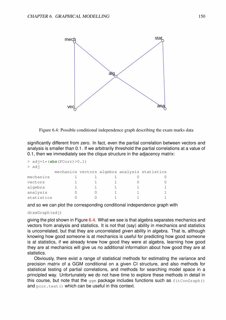
CHAPTER 6. GRAPHICAL MODELLING 150
●
●
●
●
●mech
vec
alg
ana
stat
Figure 6.4: Possible conditional independence graph describing the exam marks data
significantly different from zero. In fact, even the partial correlation between vectors andanalysis is smaller than 0.1. If we arbitrarily threshold the partial correlations at a value of0.1, then we immediately see the clique structure in the adjacency matrix:
> adj=1*(abs(PCorr)>0.1)> adj
mechanics vectors algebra analysis statisticsmechanics 1 1 1 0 0vectors 1 1 1 0 0algebra 1 1 1 1 1analysis 0 0 1 1 1statistics 0 0 1 1 1
and so we can plot the corresponding conditional independence graph with
drawGraph(adj)
giving the plot shown in Figure 6.4. What we see is that algebra separates mechanics andvectors from analysis and statistics. It is not that (say) ability in mechanics and statisticsis uncorrelated, but that they are uncorrelated given ability in algebra. That is, althoughknowing how good someone is at mechanics is useful for predicting how good someoneis at statistics, if we already knew how good they were at algebra, learning how goodthey are at mechanics will give us no additional information about how good they are atstatistics.
Obviously, there exist a range of statistical methods for estimating the variance andprecision matrix of a GGM conditional on a given CI structure, and also methods forstatistical testing of partial correlations, and methods for searching model space in aprincipled way. Unfortunately we do not have time to explore these methods in detail inthis course, but note that the ggm package includes functions such as fitConGraph()
and pcor.test() which can be useful in this context.

CHAPTER 6. GRAPHICAL MODELLING 151
●●
●
●
●
east.westnorth.south
angle
radial.position
velocity
Figure 6.5: Possible conditional independence graph describing the galaxy data
Example: galaxy data
Before moving on, it is worth looking briefly at the conditional independence structureof the variables in the galaxy data from the ElemStatLearn package. We can followthe procedure used above for the exam marks, as follows, leading to the plot shown inFigure 6.5.
> require(ElemStatLearn)> Sigma=var(galaxy)> PCorr=parcor(Sigma)> round(PCorr,digits=2)
east.west north.south angle radial.position velocityeast.west 1.00 0.37 -0.04 0.80 0.14north.south 0.37 1.00 0.15 -0.03 -0.88angle -0.04 0.15 1.00 -0.05 0.16radial.position 0.80 -0.03 -0.05 1.00 0.30velocity 0.14 -0.88 0.16 0.30 1.00> adj=1*(abs(PCorr)>0.1)> drawGraph(adj)
See section 17.3 (p.630) of [HTF] for further details of estimating undirected GGMsfrom data.
CHAPTER 6. GRAPHICAL MODELLING 152
6.5 Directed acyclic graph (DAG) models
6.5.1 Introduction
Given a conditional independence statement such as X⊥⊥Y |Z, we know that the jointdensity for the variables X, Y and Z must factorise in a special way, but it does not tellus what exactly the “natural” factorisation is. For example, given the above statement, thefollowing three factorisations are all consistent with the conditional independence state-ment:
f(x, y, z) = f(x)f(z|x)f(y|z)
f(x, y, z) = f(y)f(z|y)f(x|z)
f(x, y, z) = f(z)f(x|z)f(y|z).
But these factorisations are different, and in the context of conditionally specified statisti-cal models, one of these choices may be much more natural or convenient than another.In many applications, a particular choice of factorisation will be needed, and so it is usefulto have a method of encoding a particular factorisation and associated conditional inde-pendence statements in a formal way. This turns out to be very convenient using directedacyclic graphs (DAGs).
6.5.2 Directed graphs
A directed graph, or digraph, G, is a tuple (V,E) where V is a finite set of vertices and E aset of directed edges, with each edge e ∈ E being an ordered pair of the form e = (vi, vj),vi, vj ∈ V , i 6= j, representing an edge from vi to vj, often written vi → vj. ClearlyE ⊆ V × V = V 2.
A directed path is a sequence x0, x1, . . . , xm ∈ V such that xi−1 → xi, i = 1, 2, . . . ,m.A directed cycle is a (non-trivial) directed path starting and ending at the same vertex.
A directed acyclic graph (DAG) is a digraph which does not contain any directed cycles.DAGs turn out to be a very important concept in many areas of discrete mathematics andcomputing science.
x is a parent of y if x → y. The set of all parents of a node y is denoted pa(y). x is achild of y if y → x. The set of all children of a node y is denoted ch(y).
If there exists a directed path from x to y, then x is said to be an ancestor of y, andy is said to be a descendant of x. The set of all ancestors of a node y is written an(y),and the set of all descendants of a node x is written de(x). The non-descendants of xare defined by nd(x) ≡ V \{x ∪ de(x)}. Note that for a DAG, we must have an(x) ⊆ nd(x)(easy exercise).
A list ordering of a DAG is a sequential ordering of the nodes, x1, x2, . . . , xp in such away that xi ∈ an(xj) ⇒ i < j. A list ordering can always be constructed for a DAG, butthey are usually not unique.
Example: toy DAG
Consider the graph G = (V,E), where V = {X, Y, Z} and E = {(X,Z), (Z, Y )}. We canplot this in R using

CHAPTER 6. GRAPHICAL MODELLING 153
●●
●
ZX
Y
Figure 6.6: Simple DAG with 3 nodes and 2 edges
drawGraph(DAG(Z∼ X,Y∼ Z))
giving the graph shown in Figure 6.6. Note, for example, that Z is a child of X and aparent of Y . Similarly, Y is a descendant of X and X is an ancestor of Y . Also note thathere, an(Y ) = nd(Y ) = {X,Z}. X,Z, Y is a directed path, but Y, Z,X is not. Similarly,X,Z, Y is the only valid list ordering for this DAG.
From a DAG G, it is possible to construct an associated undirected graph, Gm, knownas the moral graph of G, by joining (marrying) all pairs of parents of each node, and thendropping arrows from all edges. This graph has the property that for each node v andits parents, pa(v) in the DAG, the corresponding subgraph in the moral graph induced byv ∪ pa(v) is complete. The marrying of parents ensures that this is the case, and is a keyproperty of the moral graph, as we shall see.
Example: toy DAG
For the simple toy DAG previously considered, each node has just one parent, so noparents need marrying, and the moral graph is obtained simply by dropping arrows fromthe DAG.
6.5.3 DAG models
As with undirected graphs, we now wish to associate factorisation and conditional inde-pendence properties of random variables with graphs, and as for the undirected case,there are several ways to do this. We consider the two most fundamental here.

CHAPTER 6. GRAPHICAL MODELLING 154
Definition 14 We say that the DAG G has the recursive factorisation or directed factori-sation (DF) property if the joint density of the random variables factorises in the form
f(x) =∏v∈V
f(v| pa(v)).
Models constructed in this way are sometimes referred to as Bayesian networks, due totheir occurrence in many applications of Bayesian inference.
Example: toy DAG
For the DAG we have been considering, the implied factorisation is
f(x, y, z) = f(x)f(z|x)f(y|z).
Definition 15 We say that the DAG G has the directed local (DL) Markov property if forall v ∈ V we have
v⊥⊥ nd(v)|pa(v).
Example: toy DAG
For the DAG we have been considering, the only non-trivial implied CI statement is
Y⊥⊥(X,Z)|Z,
or equivalently,Y⊥⊥X|Z.
Lemma 1 (DF)⇒ (DL).
ProofWe assume (DF), and pick an arbitrary u ∈ V . We wish to show that u⊥⊥ nd(u)|pa(u).
First partition V = u ∪ nd(u) ∪ de(u), and write our factorisation in the form
f(x) = f(u| pa(u))∏
v∈nd(u)
f(v| pa(v))∏
v∈de(u)
f(v| pa(v)).
We are not interested in the descendants of u, so we can marginalise those away to leave
f(u ∪ nd(u)) = f(u| pa(u))∏
v∈nd(u)
f(v| pa(v)).
But now the only term involving u is the first, giving
f(u| nd(u)) = f(u| pa(u)),
or in other words, u⊥⊥ nd(u)|pa(u). �

CHAPTER 6. GRAPHICAL MODELLING 155
Lemma 2 (DL)⇒ (DF).
Proof
Start with a list ordering of the nodes x1, x2, . . . , xp, then fac-torise the joint density in the form
f (x) = f (x1)f (x2|x1) · · · f (xp|x1, . . . , xp−1)
=
p∏i=1
f (xi|x1, . . . , xi−1).
Considering the ith term in this product, we know that since wehave a list ordering we must have {x1, . . . , xi−1} ⊆ nd(xi), andsince we are assuming that xi⊥⊥ nd(xi)|pa(xi), we have thatxi⊥⊥x1, . . . , xi−1|pa(xi), and so f (xi|x1, . . . , xi−1) = f (xi| pa(xi)),giving the factorisation
f (x) =
p∏i=1
f (xi| pa(xi)),
and so (DF) is satisfied.�
Therefore the two properties we have considered are equivalent.
Proposition 39 (DF)⇔ (DL).
We now link DAG models back to undirected graphical models via the moral graph.
Proposition 40 If the DAG G satisfies (DF), then the associated moral graph Gm satisfies(F).
Proof
We start with the factorisation
f (x) =
p∏i=1
f (xi| pa(xi))
=
p∏i=1
hi(xi, pa(xi)),
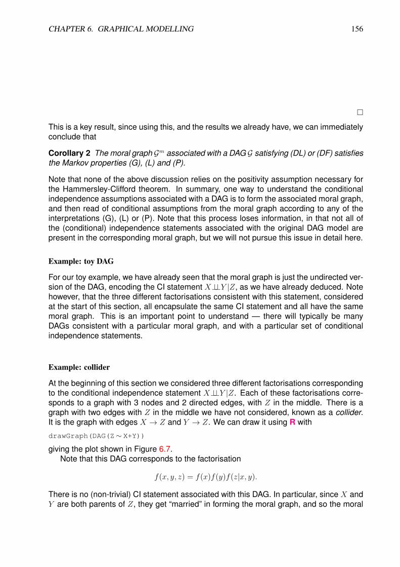
CHAPTER 6. GRAPHICAL MODELLING 156
but by construction of the moral graph, xi ∪ pa(xi) is completein Gm, and hence will be contained in a clique of Gm. By allo-cating each term to a clique, we see that the density factorisesaccording to the clique structure of Gm, and (F) is satisfied.
�
This is a key result, since using this, and the results we already have, we can immediatelyconclude that
Corollary 2 The moral graph Gm associated with a DAG G satisfying (DL) or (DF) satisfiesthe Markov properties (G), (L) and (P).
Note that none of the above discussion relies on the positivity assumption necessary forthe Hammersley-Clifford theorem. In summary, one way to understand the conditionalindependence assumptions associated with a DAG is to form the associated moral graph,and then read of conditional assumptions from the moral graph according to any of theinterpretations (G), (L) or (P). Note that this process loses information, in that not all ofthe (conditional) independence statements associated with the original DAG model arepresent in the corresponding moral graph, but we will not pursue this issue in detail here.
Example: toy DAG
For our toy example, we have already seen that the moral graph is just the undirected ver-sion of the DAG, encoding the CI statement X⊥⊥Y |Z, as we have already deduced. Notehowever, that the three different factorisations consistent with this statement, consideredat the start of this section, all encapsulate the same CI statement and all have the samemoral graph. This is an important point to understand — there will typically be manyDAGs consistent with a particular moral graph, and with a particular set of conditionalindependence statements.
Example: collider
At the beginning of this section we considered three different factorisations correspondingto the conditional independence statement X⊥⊥Y |Z. Each of these factorisations corre-sponds to a graph with 3 nodes and 2 directed edges, with Z in the middle. There is agraph with two edges with Z in the middle we have not considered, known as a collider.It is the graph with edges X → Z and Y → Z. We can draw it using R with
drawGraph(DAG(Z∼ X+Y))
giving the plot shown in Figure 6.7.Note that this DAG corresponds to the factorisation
f(x, y, z) = f(x)f(y)f(z|x, y).
There is no (non-trivial) CI statement associated with this DAG. In particular, since X andY are both parents of Z, they get “married” in forming the moral graph, and so the moral
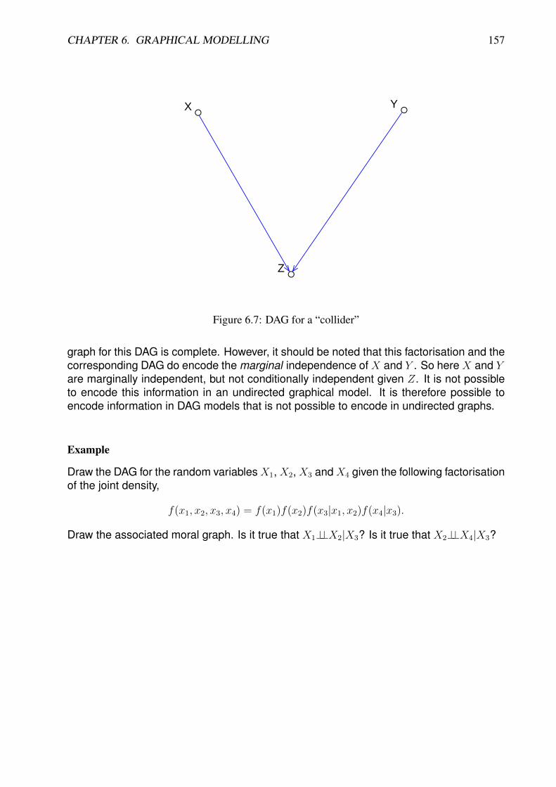
CHAPTER 6. GRAPHICAL MODELLING 157
●
● ●
Z
X Y
Figure 6.7: DAG for a “collider”
graph for this DAG is complete. However, it should be noted that this factorisation and thecorresponding DAG do encode the marginal independence of X and Y . So here X and Yare marginally independent, but not conditionally independent given Z. It is not possibleto encode this information in an undirected graphical model. It is therefore possible toencode information in DAG models that is not possible to encode in undirected graphs.
Example
Draw the DAG for the random variablesX1, X2, X3 andX4 given the following factorisationof the joint density,
f(x1, x2, x3, x4) = f(x1)f(x2)f(x3|x1, x2)f(x4|x3).
Draw the associated moral graph. Is it true that X1⊥⊥X2|X3? Is it true that X2⊥⊥X4|X3?
Can draw DAG with drawGraph(DAG(x3∼x1+x2,x4∼x3)). Can drawmoral graph with drawGraph(UG(∼x1*x2*x3+x3*x4)).
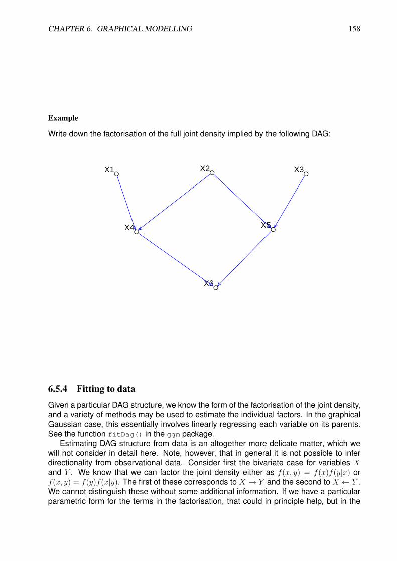
CHAPTER 6. GRAPHICAL MODELLING 158
It is not true that X1⊥⊥X2|X3, since X1 and X2 are married inthe moral graph. It is true that X2⊥⊥X4|X3, since X3 separatesX2 and X4 in the moral graph.
Example
Write down the factorisation of the full joint density implied by the following DAG:
●
● ●
●
●
●
X4
X1 X2
X5
X3
X6
f (x) = f (x1)f (x2)f (x3)f (x4|x1, x2)f (x5|x2, x3)f (x6|x4, x5)
6.5.4 Fitting to data
Given a particular DAG structure, we know the form of the factorisation of the joint density,and a variety of methods may be used to estimate the individual factors. In the graphicalGaussian case, this essentially involves linearly regressing each variable on its parents.See the function fitDag() in the ggm package.
Estimating DAG structure from data is an altogether more delicate matter, which wewill not consider in detail here. Note, however, that in general it is not possible to inferdirectionality from observational data. Consider first the bivariate case for variables Xand Y . We know that we can factor the joint density either as f(x, y) = f(x)f(y|x) orf(x, y) = f(y)f(x|y). The first of these corresponds to X → Y and the second to X ← Y .We cannot distinguish these without some additional information. If we have a particularparametric form for the terms in the factorisation, that could in principle help, but in the

CHAPTER 6. GRAPHICAL MODELLING 159
graphical Gaussian case we assume that the variables are bivariate normal, and the twofactorisations are indistinguishable from data. In general, the best strategy is often toestimate an undirected graph structure from data, and then explore the set of directedgraphs consistent with this undirected graph, informally.
6.6 Conclusion
Graphical models are one of the most important tools in modern multivariate statisticalmodelling and analysis. In particular, they are central to Bayesian hierarchical modelling,and many modern Bayesian computational methods. We do not have time to explorethese ideas here, but the basic properties of undirected and directed graphs, and graphi-cal Gaussian models forms a foundation for further study in this area.
Note that the standard reference on the theory of graphical models is:
Lauritzen, S. L. (1996) Graphical Models, Oxford Science Publications.
Some of the material in this chapter was derived from the above text.
Chapter 7
Variable selection and multiple testing
7.1 Regularisation and variable selection
7.1.1 Introduction
Let us reconsider the problem of multiple linear regression, in the form
y = Xβ + ε,
where X is an n× p data matrix, and we choose β in order to minimise ‖ε‖2. If p is large,so that X contains many variables, there may be many choices of β that almost minimiseour loss function
L(β) = (y − Xβ)T(y − Xβ).
We know that the β minimising L(β) is given by the solution of the normal equations
XTXβ = XTy.
When n ≥ p and X has full column rank, there is a unique solution given by
β = (XTX)−1XTy.
However, if X does not have full column rank (for example, because some of the variablesare co-linear), or p > n, then XTX will not be invertible, and there will be many solutionsto the normal equations, corresponding to many different minimisers of the loss functionL(β). Even if X is full rank, if it is close to rank degenerate, then solution of the normalequations may be numerically unstable, and the “optimal” β may turn out to have poorpredictive properties.
Regularisation and variable selection are two ways to deal with the above problem,which turn out to be closely related. Regularisation is concerned with smoothing theloss function, ensuring it has a unique minimum, and “shrinking” the solution towards asensible default, often zero. Regularisation methods are often termed shrinkage methodsfor this reason. We begin by looking at the classical method of regularising regressionproblems, often known as ridge regression, or Tikhonov regularisation.
160
CHAPTER 7. VARIABLE SELECTION AND MULTIPLE TESTING 161
7.1.2 Ridge regression
There are several ways to think about ridge regression. We start by viewing it as a con-strained minimisation problem, where we now find a minimum of L(β) subject to theconstraint that ‖β‖ does not exceed some threshold size. This way we ensure that wedo not consider unrealistic choices of β. Now, we often tackle constrained optimisationproblems using a Lagrange multiplier approach. In this case we will minimise the lossfunction
Lr(β) = L(β) + λ‖β‖2,and then later use λ in order to impose the required constraint. However, this gives us adifferent, and perhaps more natural, way to think about ridge regression. We modify ourloss function in order to include a penalty term which penalises choices of β with largenorm. Small values of λ lead to small penalties, and hence solutions similar to those thatwould be obtained through regular least squares approaches. However, larger values ofλ will lead to strong penalties for β with large norm, and hence will have the effect of“shrinking” the optimal solution towards the origin. Let us now consider how to solve forthe optimal β for given fixed λ ≥ 0.
Proposition 41 The β minimising Lr(β) is given by the solution to the equations
(XTX + λ I)β = XTy.
For λ > 0, these equations are guaranteed to have a unique solution given by
β = (XTX + λ I)−1XTy.
Proof
First let us expand and simplify the loss function
Lr(β) = L(β) + λ‖β‖2
= (y − Xβ)T(y − Xβ) + λβTβ
= yTy + βTXTXβ − 2βTXTy + λβTβ
= yTy + βT(XTX + λ I)β − 2βTXTy.
Now differentiating wrt β and equating to zero gives
(XTX + λ I)β = XTy.
For λ > 0, the matrix λ I is strictly positive definite, and sinceXTX is non-negative definite, XTX + λ I is strictly positive defi-nite, and hence is invertible. This gives the final result.
�
The attraction of ridge regression is that irrespective of the column rank of X, or the relativesizes of n and p, for any λ > 0 the ridge regression has a unique solution, and for largevalues of λ, the numerical solution is computationally very stable. It is in this sense thatthe problem has been regularised.
CHAPTER 7. VARIABLE SELECTION AND MULTIPLE TESTING 162
Example: galaxy data
We can look at how to implement ridge regression using R for the galaxy data. We beingby thinking about regressing velocity on the other 4 variables, and start using lm().
> require(ElemStatLearn)> y=galaxy[,5]> X=as.matrix(galaxy[,-5])> lm(y∼ X)
Call:lm(formula = y ∼ X)
Coefficients:(Intercept) Xeast.west Xnorth.south Xangle
1589.4229 0.7741 -3.1918 0.1245Xradial.position
0.9012
As usual, we can append a column of 1s to the front of X and then compute the leastsquares solution either using lm() or by solving the normal equations directly.
> X0=cbind(rep(1,length(y)),X)> lm(y∼ 0+X0)
Call:lm(formula = y ∼ 0 + X0)
Coefficients:X0 X0east.west X0north.south
X0angle1589.4229 0.7741 -3.1918
0.1245X0radial.position
0.9012
> solve(t(X0)%*%X0,t(X0)%*%y)[,1]
1589.4229455east.west 0.7740997north.south -3.1917877angle 0.1245414radial.position 0.9011797> QR=qr(X0)> solve(qr.R(QR),t(qr.Q(QR))%*%y)
[,1]1589.4229455
east.west 0.7740997north.south -3.1917877angle 0.1245414radial.position 0.9011797

CHAPTER 7. VARIABLE SELECTION AND MULTIPLE TESTING 163
We can avoid the complications associated with intercepts by first centering the outputand the predictor matrix.
> y=y-mean(y)> W=sweep(X,2,colMeans(X))> solve(t(W)%*%W,t(W)%*%y)
[,1]east.west 0.7740997north.south -3.1917877angle 0.1245414radial.position 0.9011797>> QR=qr(W)> solve(qr.R(QR),t(qr.Q(QR))%*%y)
[,1]east.west 0.7740997north.south -3.1917877angle 0.1245414radial.position 0.9011797
We can now carry out ridge regression (with λ = 100) by direct solution of the regularisednormal equations
> solve(t(W)%*%W+100*diag(4),t(W)%*%y)[,1]
east.west 0.7646416north.south -3.1881190angle 0.1244684radial.position 0.9059122
We see that the predictor is very similar to the usual least squares solution, but the addi-tion of a diagonal term will ensure that the numerical solution of the equations will be verystable. Note that we could also compute the optimal predictor by numerically optimisingthe loss function.
> loss<-function(beta)+ {+ eps=y-W%*%beta+ return(sum(eps*eps)+lambda1*sum(abs(beta))+lambda2*sum(beta*beta))+ }> lambda1=0> lambda2=0> optim(rep(0,4),loss,control=list(maxit=10000,reltol=1e-12))$par[1] 0.7740986 -3.1917888 0.1245412 0.9011769
$value[1] 288650.8
$countsfunction gradient
537 NA
CHAPTER 7. VARIABLE SELECTION AND MULTIPLE TESTING 164
$convergence[1] 0
$messageNULL
Note that in the case lambda1=0, the loss is exactly as we require for ridge regression.The other term in this loss will be explained in the following section. Note that directnumerical optimisation of multivariate functions is fraught with difficulty, and so whenevera direct alternative exists, it is almost always to be preferred. In this case, direct solutionof the regularised normal equations is a much better way to compute the solution.
7.1.3 The LASSO and variable selection
Ridge regression is one way to regularise an ill-conditioned least squares problem, butby no means the only one. In the case of p being large, another obvious approach wouldbe to select just a subset of the available variables. The intuition here is that if there aremany variables, it is likely that not all will be useful for predicting y, and that since vari-ables are likely to be correlated anyway, it will not be necessary to include all variables inthe regression even if all happen to be marginally predictive, since the column span of thesubset of variables will be similar to that of a larger subset if the variables dropped arehighly correlated with some of those that remain. There are many possible approaches tovariable selection, including forwards and backwards selection. Perhaps initially variableselection may appear to have little to do with penalised regularisation methods, but this isnot the case, and the connection between them becomes clear in the context of a regular-isation method known as the LASSO (least absolute shrinkage and selection operator),which is actually rather closely related to the method of ridge regression we have alreadyconsidered.
The Lasso uses the penalty
Ll(β) = L(β) + λ‖β‖1,
where
‖β‖1 =
p∑i=1
|βi|
is the l1-norm of β. The switch from 2-norm to 1-norm seems at first to be unlikely to makea significant difference to the shrinkage behaviour of the estimator, but in fact it does, andimportantly, encourages “sparsity” in the optimal solution. It also complicates analysissomewhat, since it is no longer possible to compute a simple closed-form solution for theoptimal β, and since the l1-norm is not everywhere differentiable (it is not differentiableon the coordinate axes), methods of optimisation which assume smooth functions cannotbe used. In fact, it is precisely this lack of differentiability of the l1-norm on the axeswhich causes the method to often have minima including components of β which areexactly zero. Zeroes in the optimal β correspond to variables which are dropped outof the regression, and similarly, the non-zero elements of β correspond to the selectedvariables. Thus, the simple switch from an l2 to an l1 regularisation penalty leads directlyto a method which simultaneously regularises and selects variables for analysis.
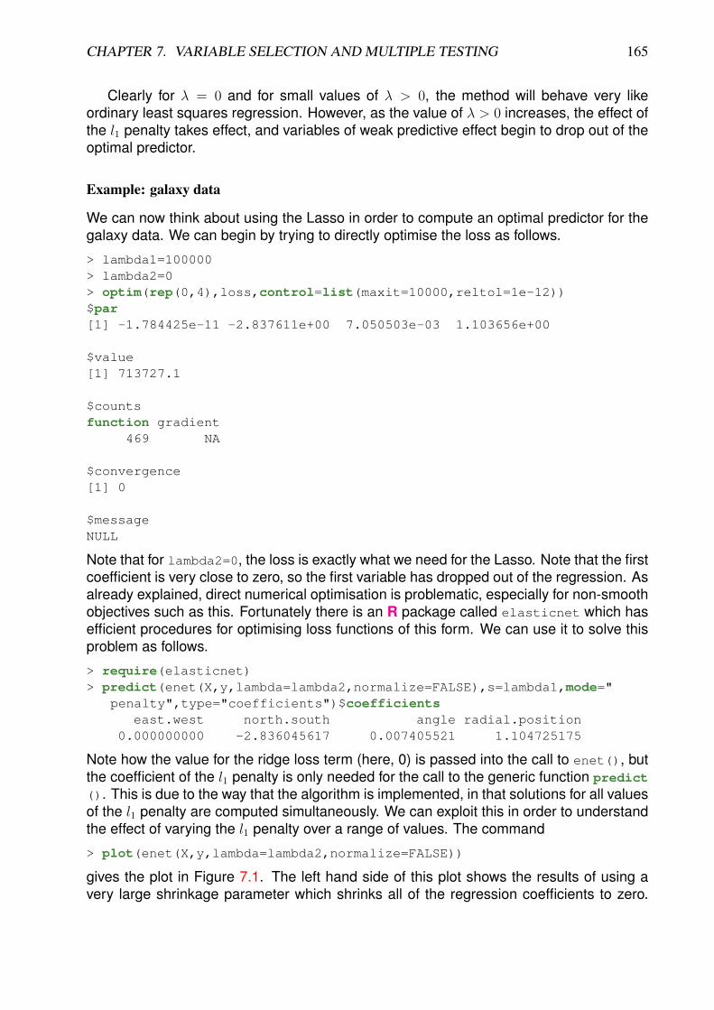
CHAPTER 7. VARIABLE SELECTION AND MULTIPLE TESTING 165
Clearly for λ = 0 and for small values of λ > 0, the method will behave very likeordinary least squares regression. However, as the value of λ > 0 increases, the effect ofthe l1 penalty takes effect, and variables of weak predictive effect begin to drop out of theoptimal predictor.
Example: galaxy data
We can now think about using the Lasso in order to compute an optimal predictor for thegalaxy data. We can begin by trying to directly optimise the loss as follows.
> lambda1=100000> lambda2=0> optim(rep(0,4),loss,control=list(maxit=10000,reltol=1e-12))$par[1] -1.784425e-11 -2.837611e+00 7.050503e-03 1.103656e+00
$value[1] 713727.1
$countsfunction gradient
469 NA
$convergence[1] 0
$messageNULL
Note that for lambda2=0, the loss is exactly what we need for the Lasso. Note that the firstcoefficient is very close to zero, so the first variable has dropped out of the regression. Asalready explained, direct numerical optimisation is problematic, especially for non-smoothobjectives such as this. Fortunately there is an R package called elasticnet which hasefficient procedures for optimising loss functions of this form. We can use it to solve thisproblem as follows.
> require(elasticnet)> predict(enet(X,y,lambda=lambda2,normalize=FALSE),s=lambda1,mode="
penalty",type="coefficients")$coefficientseast.west north.south angle radial.position
0.000000000 -2.836045617 0.007405521 1.104725175
Note how the value for the ridge loss term (here, 0) is passed into the call to enet(), butthe coefficient of the l1 penalty is only needed for the call to the generic function predict(). This is due to the way that the algorithm is implemented, in that solutions for all valuesof the l1 penalty are computed simultaneously. We can exploit this in order to understandthe effect of varying the l1 penalty over a range of values. The command
> plot(enet(X,y,lambda=lambda2,normalize=FALSE))
gives the plot in Figure 7.1. The left hand side of this plot shows the results of using avery large shrinkage parameter which shrinks all of the regression coefficients to zero.
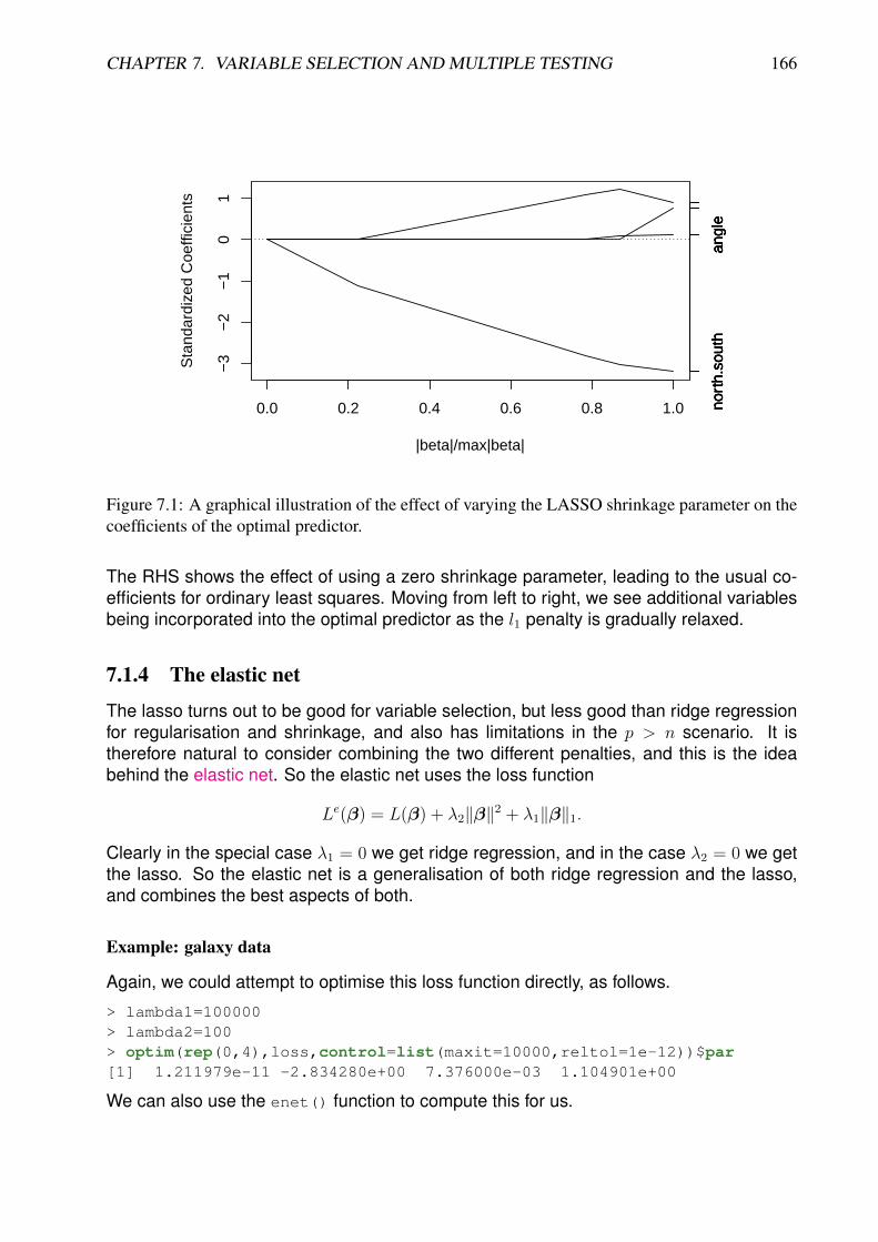
CHAPTER 7. VARIABLE SELECTION AND MULTIPLE TESTING 166
0.0 0.2 0.4 0.6 0.8 1.0
−3
−2
−1
01
|beta|/max|beta|
Sta
ndar
dize
d C
oeffi
cien
ts
nort
h.so
uth
angl
eno
rth.
sout
han
gle
nort
h.so
uth
angl
eno
rth.
sout
han
gle
Figure 7.1: A graphical illustration of the effect of varying the LASSO shrinkage parameter on thecoefficients of the optimal predictor.
The RHS shows the effect of using a zero shrinkage parameter, leading to the usual co-efficients for ordinary least squares. Moving from left to right, we see additional variablesbeing incorporated into the optimal predictor as the l1 penalty is gradually relaxed.
7.1.4 The elastic net
The lasso turns out to be good for variable selection, but less good than ridge regressionfor regularisation and shrinkage, and also has limitations in the p > n scenario. It istherefore natural to consider combining the two different penalties, and this is the ideabehind the elastic net. So the elastic net uses the loss function
Le(β) = L(β) + λ2‖β‖2 + λ1‖β‖1.
Clearly in the special case λ1 = 0 we get ridge regression, and in the case λ2 = 0 we getthe lasso. So the elastic net is a generalisation of both ridge regression and the lasso,and combines the best aspects of both.
Example: galaxy data
Again, we could attempt to optimise this loss function directly, as follows.
> lambda1=100000> lambda2=100> optim(rep(0,4),loss,control=list(maxit=10000,reltol=1e-12))$par[1] 1.211979e-11 -2.834280e+00 7.376000e-03 1.104901e+00
We can also use the enet() function to compute this for us.
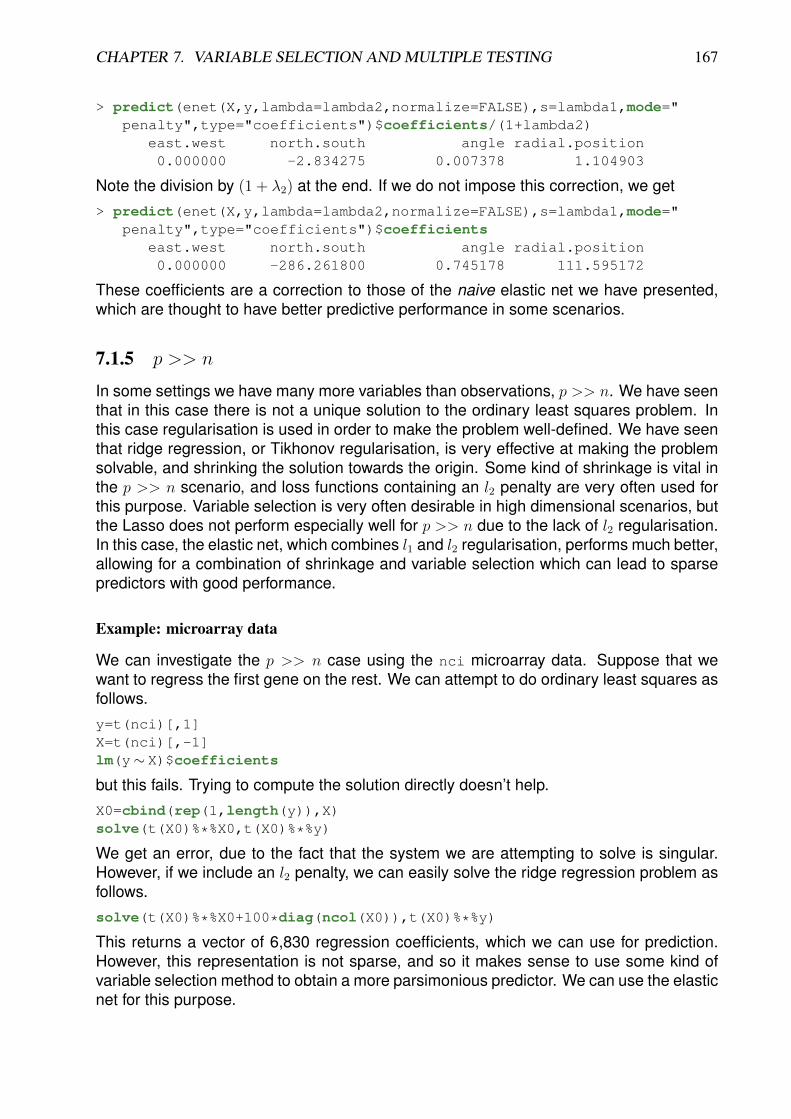
CHAPTER 7. VARIABLE SELECTION AND MULTIPLE TESTING 167
> predict(enet(X,y,lambda=lambda2,normalize=FALSE),s=lambda1,mode="penalty",type="coefficients")$coefficients/(1+lambda2)
east.west north.south angle radial.position0.000000 -2.834275 0.007378 1.104903
Note the division by (1 + λ2) at the end. If we do not impose this correction, we get> predict(enet(X,y,lambda=lambda2,normalize=FALSE),s=lambda1,mode="
penalty",type="coefficients")$coefficientseast.west north.south angle radial.position0.000000 -286.261800 0.745178 111.595172
These coefficients are a correction to those of the naive elastic net we have presented,which are thought to have better predictive performance in some scenarios.
7.1.5 p >> n
In some settings we have many more variables than observations, p >> n. We have seenthat in this case there is not a unique solution to the ordinary least squares problem. Inthis case regularisation is used in order to make the problem well-defined. We have seenthat ridge regression, or Tikhonov regularisation, is very effective at making the problemsolvable, and shrinking the solution towards the origin. Some kind of shrinkage is vital inthe p >> n scenario, and loss functions containing an l2 penalty are very often used forthis purpose. Variable selection is very often desirable in high dimensional scenarios, butthe Lasso does not perform especially well for p >> n due to the lack of l2 regularisation.In this case, the elastic net, which combines l1 and l2 regularisation, performs much better,allowing for a combination of shrinkage and variable selection which can lead to sparsepredictors with good performance.
Example: microarray data
We can investigate the p >> n case using the nci microarray data. Suppose that wewant to regress the first gene on the rest. We can attempt to do ordinary least squares asfollows.y=t(nci)[,1]X=t(nci)[,-1]lm(y∼ X)$coefficients
but this fails. Trying to compute the solution directly doesn’t help.X0=cbind(rep(1,length(y)),X)solve(t(X0)%*%X0,t(X0)%*%y)
We get an error, due to the fact that the system we are attempting to solve is singular.However, if we include an l2 penalty, we can easily solve the ridge regression problem asfollows.solve(t(X0)%*%X0+100*diag(ncol(X0)),t(X0)%*%y)
This returns a vector of 6,830 regression coefficients, which we can use for prediction.However, this representation is not sparse, and so it makes sense to use some kind ofvariable selection method to obtain a more parsimonious predictor. We can use the elasticnet for this purpose.
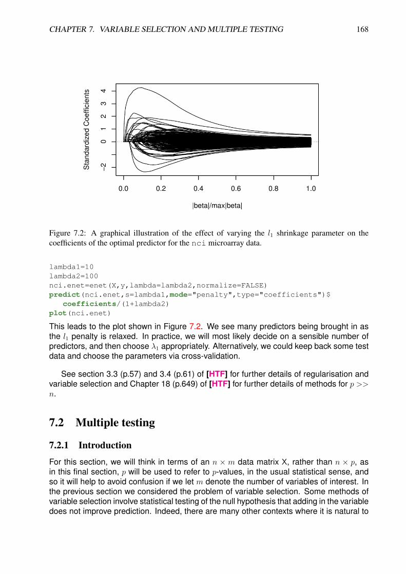
CHAPTER 7. VARIABLE SELECTION AND MULTIPLE TESTING 168
Figure 7.2: A graphical illustration of the effect of varying the l1 shrinkage parameter on thecoefficients of the optimal predictor for the nci microarray data.
lambda1=10lambda2=100nci.enet=enet(X,y,lambda=lambda2,normalize=FALSE)predict(nci.enet,s=lambda1,mode="penalty",type="coefficients")$
coefficients/(1+lambda2)plot(nci.enet)
This leads to the plot shown in Figure 7.2. We see many predictors being brought in asthe l1 penalty is relaxed. In practice, we will most likely decide on a sensible number ofpredictors, and then choose λ1 appropriately. Alternatively, we could keep back some testdata and choose the parameters via cross-validation.
See section 3.3 (p.57) and 3.4 (p.61) of [HTF] for further details of regularisation andvariable selection and Chapter 18 (p.649) of [HTF] for further details of methods for p >>n.
7.2 Multiple testing
7.2.1 Introduction
For this section, we will think in terms of an n × m data matrix X, rather than n × p, asin this final section, p will be used to refer to p-values, in the usual statistical sense, andso it will help to avoid confusion if we let m denote the number of variables of interest. Inthe previous section we considered the problem of variable selection. Some methods ofvariable selection involve statistical testing of the null hypothesis that adding in the variabledoes not improve prediction. Indeed, there are many other contexts where it is natural to

CHAPTER 7. VARIABLE SELECTION AND MULTIPLE TESTING 169
apply a test to each variable separately in a multivariate problem. This is particularlycommon in genomics, where statistical tests are often applied to each variable in turn,in order to find genes which behave significantly differently in some appropriate sense.In this context, we often end up with a p-value associated with each variable (each genein the genomic data context), and need to somehow threshold these p-values in orderto produce a list of significant variables. The p-value is the probability (under repeatedsampling) that a test statistic as extreme as that observed, will be observed, assumingthat the null hypothesis is true.
7.2.2 The multiple testing problem
We typically consider some threshold significance level, α (often α = 0.05 for a singletest), and then flag as “significant” tests with a p-value smaller than α. There are manyissues with this, but here we will focus on the problems which arise when many tests areconsidered together (here, m). In order to get a simple understanding of the problem, wewill assume that all of the tests are independent, although in practice this is unlikely to bethe case.
If we carry outm tests, even if the null hypothesis is true in every case, so that we wouldnot wish any tests to be flagged as significant, we know that by construction, each of them tests will be significant with probability α. In this case the number of false positives willbe X, where X ∼ Bin(m,α). Then we have E(X) = mα, so for large m we expect toget many false positive tests. For example, for m = 7, 000 and α = 0.05, we would expectto get 350 false positives in the case where there are no true positives. Indeed, if weanticipate the number of true positives to be small, will will a priori expect that most of thepositive tests will in fact be false positives, and we will have no way to decide on which orhow many of these we should consider. This is the multiple testing problem.
7.2.3 Bonferroni correction
The Bonferroni method is the classical solution to multiple testing. For a collection of (in-dependent) tests, Bonferroni’s method controls the family-wise error rate (FWER) — thisis the probability of at least one false positive when there are no true positives. Therefore
FWER = P(At least one false positive)
= 1− P(No false positives)
= 1− (1− α)m
Now, for small α, (1− α)m ' 1−mα (first 2 terms in binomial expansion), and so
FWER ' mα.
Note that although we have derived this as an approximation, and assuming independenttests, it is possible to deduce directly using Boole’s inequality that
FWER ≤ mα,
without assuming independence or making any approximation. Either way, if a FWER ofα′ is required, choosing a significance level for the individual tests of α = α′/m will achieve
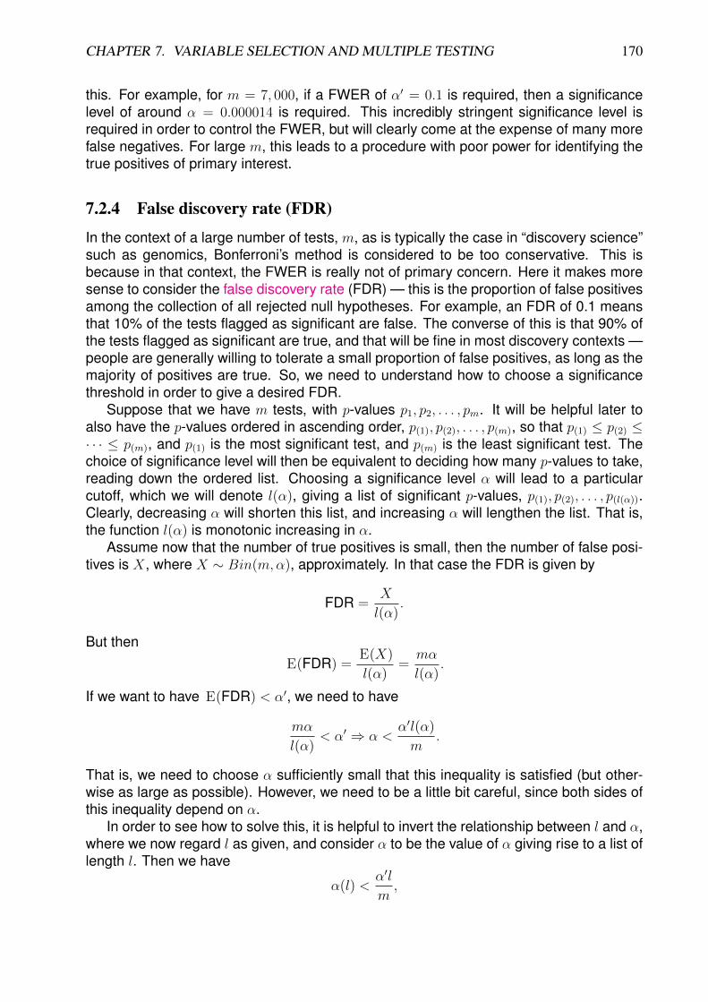
CHAPTER 7. VARIABLE SELECTION AND MULTIPLE TESTING 170
this. For example, for m = 7, 000, if a FWER of α′ = 0.1 is required, then a significancelevel of around α = 0.000014 is required. This incredibly stringent significance level isrequired in order to control the FWER, but will clearly come at the expense of many morefalse negatives. For large m, this leads to a procedure with poor power for identifying thetrue positives of primary interest.
7.2.4 False discovery rate (FDR)
In the context of a large number of tests, m, as is typically the case in “discovery science”such as genomics, Bonferroni’s method is considered to be too conservative. This isbecause in that context, the FWER is really not of primary concern. Here it makes moresense to consider the false discovery rate (FDR) — this is the proportion of false positivesamong the collection of all rejected null hypotheses. For example, an FDR of 0.1 meansthat 10% of the tests flagged as significant are false. The converse of this is that 90% ofthe tests flagged as significant are true, and that will be fine in most discovery contexts —people are generally willing to tolerate a small proportion of false positives, as long as themajority of positives are true. So, we need to understand how to choose a significancethreshold in order to give a desired FDR.
Suppose that we have m tests, with p-values p1, p2, . . . , pm. It will be helpful later toalso have the p-values ordered in ascending order, p(1), p(2), . . . , p(m), so that p(1) ≤ p(2) ≤· · · ≤ p(m), and p(1) is the most significant test, and p(m) is the least significant test. Thechoice of significance level will then be equivalent to deciding how many p-values to take,reading down the ordered list. Choosing a significance level α will lead to a particularcutoff, which we will denote l(α), giving a list of significant p-values, p(1), p(2), . . . , p(l(α)).Clearly, decreasing α will shorten this list, and increasing α will lengthen the list. That is,the function l(α) is monotonic increasing in α.
Assume now that the number of true positives is small, then the number of false posi-tives is X, where X ∼ Bin(m,α), approximately. In that case the FDR is given by
FDR =X
l(α).
But thenE(FDR) =
E(X)
l(α)=mα
l(α).
If we want to have E(FDR) < α′, we need to have
mα
l(α)< α′ ⇒ α <
α′l(α)
m.
That is, we need to choose α sufficiently small that this inequality is satisfied (but other-wise as large as possible). However, we need to be a little bit careful, since both sides ofthis inequality depend on α.
In order to see how to solve this, it is helpful to invert the relationship between l and α,where we now regard l as given, and consider α to be the value of α giving rise to a list oflength l. Then we have
α(l) <α′l
m,
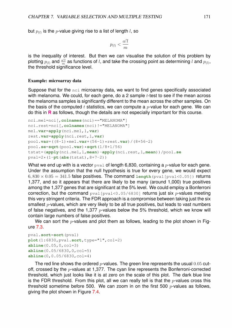
CHAPTER 7. VARIABLE SELECTION AND MULTIPLE TESTING 171
but p(l) is the p-value giving rise to a list of length l, so
p(l) <α′l
m
is the inequality of interest. But then we can visualise the solution of this problem byplotting p(l) and α′l
mas functions of l, and take the crossing point as determining l and p(l),
the threshold significance level.
Example: microarray data
Suppose that for the nci microarray data, we want to find genes specifically associatedwith melanoma. We could, for each gene, do a 2 sample t-test to see if the mean acrossthe melanoma samples is significantly different to the mean across the other samples. Onthe basis of the computed t statistics, we can compute a p-value for each gene. We cando this in R as follows, though the details are not especially important for this course.
nci.mel=nci[,colnames(nci)=="MELANOMA"]nci.rest=nci[,colnames(nci)!="MELANOMA"]mel.var=apply(nci.mel,1,var)rest.var=apply(nci.rest,1,var)pool.var=((8-1)*mel.var+(56-1)*rest.var)/(8+56-2)pool.se=sqrt(pool.var)*sqrt(1/8+1/56)tstat=(apply(nci.mel,1,mean)-apply(nci.rest,1,mean))/pool.sepval=2*(1-pt(abs(tstat),8+7-2))
What we end up with is a vector pval of length 6,830, containing a p-value for each gene.Under the assumption that the null hypothesis is true for every gene, we would expect6, 830 × 0.05 = 341.5 false positives. The command length(pval[pval<0.05]) returns1,377, and so it appears that there are likely to be many (around 1,000) true positivesamong the 1,377 genes that are significant at the 5% level. We could employ a Bonferronicorrection, but the command pval[pval<0.05/6830] returns just six p-values meetingthis very stringent criteria. The FDR approach is a compromise between taking just the sixsmallest p-values, which are very likely to be all true positives, but leads to vast numbersof false negatives, and the 1,377 p-values below the 5% threshold, which we know willcontain large numbers of false positives.
We can sort the p-values and plot them as follows, leading to the plot shown in Fig-ure 7.3.
pval.sort=sort(pval)plot(1:6830,pval.sort,type="l",col=2)abline(0.05,0,col=3)abline(0.05/6830,0,col=5)abline(0,0.05/6830,col=4)
The red line shows the ordered p-values. The green line represents the usual 0.05 cut-off, crossed by the p-values at 1,377. The cyan line represents the Bonferroni-correctedthreshold, which just looks like it is at zero on the scale of this plot. The dark blue lineis the FDR threshold. From this plot, all we can really tell is that the p-values cross thisthreshold sometime before 500. We can zoom in on the first 500 p-values as follows,giving the plot shown in Figure 7.4.
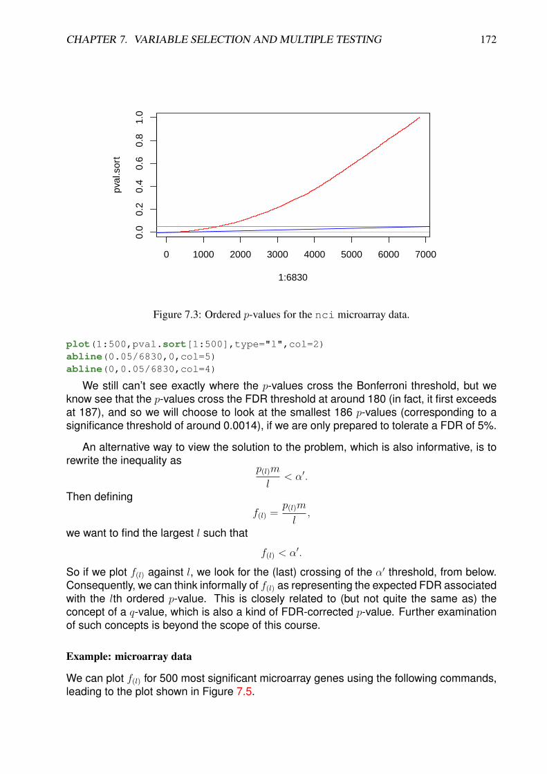
CHAPTER 7. VARIABLE SELECTION AND MULTIPLE TESTING 172
0 1000 2000 3000 4000 5000 6000 7000
0.0
0.2
0.4
0.6
0.8
1.0
1:6830
pval
.sor
t
Figure 7.3: Ordered p-values for the nci microarray data.
plot(1:500,pval.sort[1:500],type="l",col=2)abline(0.05/6830,0,col=5)abline(0,0.05/6830,col=4)
We still can’t see exactly where the p-values cross the Bonferroni threshold, but weknow see that the p-values cross the FDR threshold at around 180 (in fact, it first exceedsat 187), and so we will choose to look at the smallest 186 p-values (corresponding to asignificance threshold of around 0.0014), if we are only prepared to tolerate a FDR of 5%.
An alternative way to view the solution to the problem, which is also informative, is torewrite the inequality as
p(l)m
l< α′.
Then definingf(l) =
p(l)m
l,
we want to find the largest l such that
f(l) < α′.
So if we plot f(l) against l, we look for the (last) crossing of the α′ threshold, from below.Consequently, we can think informally of f(l) as representing the expected FDR associatedwith the lth ordered p-value. This is closely related to (but not quite the same as) theconcept of a q-value, which is also a kind of FDR-corrected p-value. Further examinationof such concepts is beyond the scope of this course.
Example: microarray data
We can plot f(l) for 500 most significant microarray genes using the following commands,leading to the plot shown in Figure 7.5.
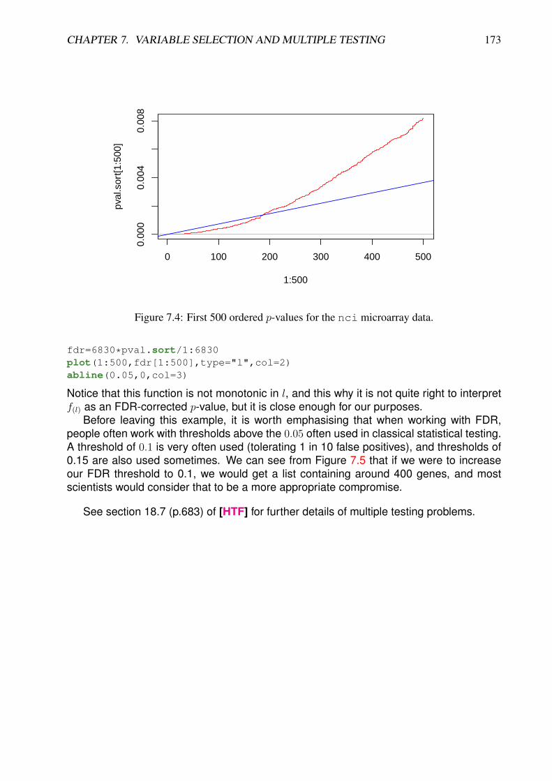
CHAPTER 7. VARIABLE SELECTION AND MULTIPLE TESTING 173
0 100 200 300 400 500
0.00
00.
004
0.00
8
1:500
pval
.sor
t[1:5
00]
Figure 7.4: First 500 ordered p-values for the nci microarray data.
fdr=6830*pval.sort/1:6830plot(1:500,fdr[1:500],type="l",col=2)abline(0.05,0,col=3)
Notice that this function is not monotonic in l, and this why it is not quite right to interpretf(l) as an FDR-corrected p-value, but it is close enough for our purposes.
Before leaving this example, it is worth emphasising that when working with FDR,people often work with thresholds above the 0.05 often used in classical statistical testing.A threshold of 0.1 is very often used (tolerating 1 in 10 false positives), and thresholds of0.15 are also used sometimes. We can see from Figure 7.5 that if we were to increaseour FDR threshold to 0.1, we would get a list containing around 400 genes, and mostscientists would consider that to be a more appropriate compromise.
See section 18.7 (p.683) of [HTF] for further details of multiple testing problems.
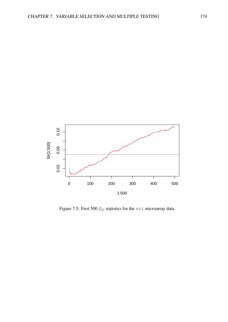
CHAPTER 7. VARIABLE SELECTION AND MULTIPLE TESTING 174
0 100 200 300 400 500
0.02
0.06
0.10
1:500
fdr[
1:50
0]
Figure 7.5: First 500 f(l) statistics for the nci microarray data.