Embed Size (px)
Citation preview

Discrete random variablesExpectation and variance
Standard discrete probability distributions
MAS113 Introduction to Probability and
Statistics
Dr Jonathan Jordan
School of Mathematics and Statistics, University of Sheffield
2017–18
Dr Jonathan Jordan MAS113 Introduction to Probability and Statistics

Discrete random variablesExpectation and variance
Standard discrete probability distributions
Random variables
Informally, we think of a random variable as any quantitythat is uncertain to us. For example:
the number of emergency call-outs received by a firestation in a given week;
the price of a barrel of oil in one month’s time;
the number of gold medals won by Great Britain at thenext summer Olympics.
Dr Jonathan Jordan MAS113 Introduction to Probability and Statistics

Discrete random variablesExpectation and variance
Standard discrete probability distributions
Random variables continued
We cannot say with certainty what any of these quantities are,but probability theory gives us a framework for describing howlikely different values are.
Whereas elements of a sample space may not be numerical,random variables are always numerical quantities, and so,when defining a random variable, we need a rule for gettingfrom the random outcome in the sample space to the value ofthe random variable.
Dr Jonathan Jordan MAS113 Introduction to Probability and Statistics

Discrete random variablesExpectation and variance
Standard discrete probability distributions
Random variables continued
Definition
Given a sample space S , we define a random variable X tobe a mapping from S to the real line R.
We sometimes write a random variable as X (s), where s ∈ S .We define the range of X to be the set of all possible valuesof X :
RX := {x ∈ R; x = X (s) for some s ∈ S}.
Dr Jonathan Jordan MAS113 Introduction to Probability and Statistics
Discrete random variablesExpectation and variance
Standard discrete probability distributions
Random variables continued
Definition
Given a sample space S , we define a random variable X tobe a mapping from S to the real line R.We sometimes write a random variable as X (s), where s ∈ S .
We define the range of X to be the set of all possible valuesof X :
RX := {x ∈ R; x = X (s) for some s ∈ S}.
Dr Jonathan Jordan MAS113 Introduction to Probability and Statistics

Discrete random variablesExpectation and variance
Standard discrete probability distributions
Random variables continued
Definition
Given a sample space S , we define a random variable X tobe a mapping from S to the real line R.We sometimes write a random variable as X (s), where s ∈ S .We define the range of X to be the set of all possible valuesof X :
RX := {x ∈ R; x = X (s) for some s ∈ S}.
Dr Jonathan Jordan MAS113 Introduction to Probability and Statistics

Discrete random variablesExpectation and variance
Standard discrete probability distributions
Discrete random variables
In this chapter, we consider discrete random variables, inwhich the number of possible values is either finite orcountably infinite.
Example
Counting heads in coin tosses
Example
Share portfolio
Dr Jonathan Jordan MAS113 Introduction to Probability and Statistics

Discrete random variablesExpectation and variance
Standard discrete probability distributions
Summation notation
Before continuing with the discussion of random variables, wedefine some new summation notation, and recap some resultsregarding manipulations of sums.
Let X be a discrete random variable with rangeRX = {x1, x2, . . . , xn}.
For any function g(x), we define
∑x∈Rx
g(x) :=n∑
i=1
g(xi) = g(x1) + g(x2) + . . . + g(xn).
Dr Jonathan Jordan MAS113 Introduction to Probability and Statistics

Discrete random variablesExpectation and variance
Standard discrete probability distributions
Summation notation continued
For any two constants a and b, we have
n∑i=1
(a + bg(xi)) = (a + bg(x1)) + . . . + (a + bg(xn))
= na + bn∑
i=1
g(xi).
Note thatn∑
i=1
a = na,
(so the sum is not equal to a).
Dr Jonathan Jordan MAS113 Introduction to Probability and Statistics

Discrete random variablesExpectation and variance
Standard discrete probability distributions
Probability mass functions
Definition
For a discrete random variable X , we define the probabilitymass function (p.m.f. for short) pX to be
pX (x) := P(X = x),
where x can be any real number.Note that P(X = x) = P(A) where
A = {s ∈ S ; X (s) = x}.
Dr Jonathan Jordan MAS113 Introduction to Probability and Statistics

Discrete random variablesExpectation and variance
Standard discrete probability distributions
Probability mass functions
Definition
For a discrete random variable X , we define the probabilitymass function (p.m.f. for short) pX to be
pX (x) := P(X = x),
where x can be any real number.
Note that P(X = x) = P(A) where
A = {s ∈ S ; X (s) = x}.
Dr Jonathan Jordan MAS113 Introduction to Probability and Statistics

Discrete random variablesExpectation and variance
Standard discrete probability distributions
Probability mass functions
Definition
For a discrete random variable X , we define the probabilitymass function (p.m.f. for short) pX to be
pX (x) := P(X = x),
where x can be any real number.Note that P(X = x) = P(A) where
A = {s ∈ S ; X (s) = x}.
Dr Jonathan Jordan MAS113 Introduction to Probability and Statistics

Discrete random variablesExpectation and variance
Standard discrete probability distributions
Notation
In the notation, we use X to represent the random variable,and x to represent a possible value of X
Whereas X refers to a specific random variable, the use of theletter x is arbitrary; we could just as well writepX (a) := P(X = a).
Dr Jonathan Jordan MAS113 Introduction to Probability and Statistics
Discrete random variablesExpectation and variance
Standard discrete probability distributions
Properties
A probability mass function must have the following twoproperties.
1 pX (x) ≥ 0∀x ∈ R.
2 Probability mass functions must ‘sum to 1’:∑x∈RX
pX (x) = 1.
Dr Jonathan Jordan MAS113 Introduction to Probability and Statistics

Discrete random variablesExpectation and variance
Standard discrete probability distributions
Proofs of properties
Property 1 follows from the definition of pX (x).
To prove property 2, first write RX = {x1, x2, . . . , xn}, and letAi = {s ∈ S ; X (s) = xi}.
You should now convince yourself that A1, . . . ,An is apartition of S .
Dr Jonathan Jordan MAS113 Introduction to Probability and Statistics

Discrete random variablesExpectation and variance
Standard discrete probability distributions
Example
Example
In a simple lottery, two numbers are drawn at random, withoutreplacement, from the numbers 1,2,3,4.You choose two numbers: 1 and 3.
If both 1 and 3 are drawn, you win £10. If either 1 or 3 isdrawn (but not both), you win £5. Otherwise, you winnothing.Let X be the amount in pounds that you win. Tabulate pX (x).
Dr Jonathan Jordan MAS113 Introduction to Probability and Statistics

Discrete random variablesExpectation and variance
Standard discrete probability distributions
Example
Example
In a simple lottery, two numbers are drawn at random, withoutreplacement, from the numbers 1,2,3,4.You choose two numbers: 1 and 3.If both 1 and 3 are drawn, you win £10. If either 1 or 3 isdrawn (but not both), you win £5. Otherwise, you winnothing.
Let X be the amount in pounds that you win. Tabulate pX (x).
Dr Jonathan Jordan MAS113 Introduction to Probability and Statistics

Discrete random variablesExpectation and variance
Standard discrete probability distributions
Example
Example
In a simple lottery, two numbers are drawn at random, withoutreplacement, from the numbers 1,2,3,4.You choose two numbers: 1 and 3.If both 1 and 3 are drawn, you win £10. If either 1 or 3 isdrawn (but not both), you win £5. Otherwise, you winnothing.Let X be the amount in pounds that you win. Tabulate pX (x).
Dr Jonathan Jordan MAS113 Introduction to Probability and Statistics

Discrete random variablesExpectation and variance
Standard discrete probability distributions
Measure
Note that a probability mass function can be thought of asdefining a probability measure on the range space RX .
For a subset A ⊆ RX , define mX (A) := P(X ∈ A).
It is not hard to check that mX satisfies the definition of aprobability measure, and it is called the law or distribution ofX .
We generally think in terms of the probability mass functionrather than of the measure, but the measure idea is usefulwhen we come to generalise beyond discrete random variables.
Dr Jonathan Jordan MAS113 Introduction to Probability and Statistics

Discrete random variablesExpectation and variance
Standard discrete probability distributions
Cumulative distribution function
Definition
We define the cumulative distribution function,abbreviated to c.d.f., FX of a random variable X to be
FX (x) := P(X ≤ x),
where x can be any real number.
Dr Jonathan Jordan MAS113 Introduction to Probability and Statistics

Discrete random variablesExpectation and variance
Standard discrete probability distributions
C.d.f. and p.d.f.
The cumulative distribution function can be written in termsof the probability mass function:
FX (x) := P(X ≤ x) =∑
a≤x ,a∈RX
pX (a). (1)
Dr Jonathan Jordan MAS113 Introduction to Probability and Statistics

Discrete random variablesExpectation and variance
Standard discrete probability distributions
Example
Example
Suppose England are to play the West Indies in a 3 match testseries. Let X be the number of matches won by England. Ifmy probability mass function for X is
pX (0) = 0.05, pX (1) = 0.2, pX (2) = 0.6, pX (3) = 0.15,
tabulate my cumulative distribution function.
Dr Jonathan Jordan MAS113 Introduction to Probability and Statistics

Discrete random variablesExpectation and variance
Standard discrete probability distributions
Quantile function
The quantile function is related to the inverse of thecumulative distribution function.
Definition
For α ∈ [0, 1] the α quantile (or 100× α percentile) is thesmallest value of x such that
FX (x) ≥ α
The median is the 0.5 quantile.
Dr Jonathan Jordan MAS113 Introduction to Probability and Statistics

Discrete random variablesExpectation and variance
Standard discrete probability distributions
Independence of random variables
We say that two random variables X and Y are independentof each other if any event defined only using the value of X isindependent of any event defined only using the value of Y .
More specifically, we can make the following definition fordiscrete random variables:
Definition
Two discrete random variables X and Y are independent if
P(X = x ,Y = y) = P(X = x)P(Y = y),
for all x and y , or, equivalently, . . .
Dr Jonathan Jordan MAS113 Introduction to Probability and Statistics

Discrete random variablesExpectation and variance
Standard discrete probability distributions
Independence continued
Definition. . .
P(X = x |Y = y) = P(X = x).
If two random variables are not independent, then we say thatthey are dependent.
Dr Jonathan Jordan MAS113 Introduction to Probability and Statistics

Discrete random variablesExpectation and variance
Standard discrete probability distributions
Example
Example
Independence of random variables
Dr Jonathan Jordan MAS113 Introduction to Probability and Statistics
Discrete random variablesExpectation and variance
Standard discrete probability distributions
Expectation and variance
The probability mass function gives a complete description ofthe uncertainty we have about a random variable X .
It tells us how likely each possible value of X is.
However, there are other quantities that can tell us usefulthings about a random variable, which we can derive from theprobability mass function. We consider here the expectationand variance of a random variable.
Dr Jonathan Jordan MAS113 Introduction to Probability and Statistics

Discrete random variablesExpectation and variance
Standard discrete probability distributions
Expectation I
On a European roulette wheel, the ball can land on one of theintegers 0 to 36.
A bet of one pound on odd returns one pound (plus theoriginal stake) if the ball lands on any odd number from 1 to35.
Assuming the ball is equally likely to land anywhere, if you betone pound on odd a large number of times, how much moneyper game are you likely to win (or lose)?
Dr Jonathan Jordan MAS113 Introduction to Probability and Statistics

Discrete random variablesExpectation and variance
Standard discrete probability distributions
Expectation II
Informally, if you bet on odd 10000 times, we might supposethat you will win 18
37× 10000 = 4865 times and lose
1937× 10000 = 5135 times, so you will lose 270 pounds overall,
or 2.7 pence per game.
Formally, we define the expected profit (or loss) per game.
Dr Jonathan Jordan MAS113 Introduction to Probability and Statistics
Discrete random variablesExpectation and variance
Standard discrete probability distributions
Expectation
Definition
The expectation E (X ) of a discrete random variable X isdefined as
E (X ) :=∑x∈RX
xP(X = x)
We refer to the expectation of X as the mean of X and writeµX to represent the mean:
µX := E (X ).
Dr Jonathan Jordan MAS113 Introduction to Probability and Statistics

Discrete random variablesExpectation and variance
Standard discrete probability distributions
Example
Example
In the roulette example, let X be your net winnings after asingle bet of one pound on odd. What is E (X )?
Dr Jonathan Jordan MAS113 Introduction to Probability and Statistics

Discrete random variablesExpectation and variance
Standard discrete probability distributions
Example
Example
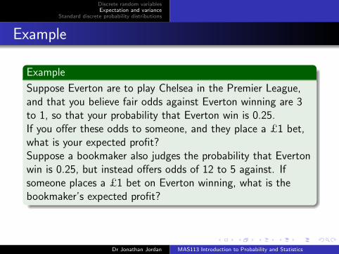
Suppose Everton are to play Chelsea in the Premier League,and that you believe fair odds against Everton winning are 3to 1, so that your probability that Everton win is 0.25.
If you offer these odds to someone, and they place a £1 bet,what is your expected profit?Suppose a bookmaker also judges the probability that Evertonwin is 0.25, but instead offers odds of 12 to 5 against. Ifsomeone places a £1 bet on Everton winning, what is thebookmaker’s expected profit?
Dr Jonathan Jordan MAS113 Introduction to Probability and Statistics

Discrete random variablesExpectation and variance
Standard discrete probability distributions
Example
Example
Suppose Everton are to play Chelsea in the Premier League,and that you believe fair odds against Everton winning are 3to 1, so that your probability that Everton win is 0.25.If you offer these odds to someone, and they place a £1 bet,what is your expected profit?
Suppose a bookmaker also judges the probability that Evertonwin is 0.25, but instead offers odds of 12 to 5 against. Ifsomeone places a £1 bet on Everton winning, what is thebookmaker’s expected profit?
Dr Jonathan Jordan MAS113 Introduction to Probability and Statistics
Discrete random variablesExpectation and variance
Standard discrete probability distributions
Example
Example
Suppose Everton are to play Chelsea in the Premier League,and that you believe fair odds against Everton winning are 3to 1, so that your probability that Everton win is 0.25.If you offer these odds to someone, and they place a £1 bet,what is your expected profit?Suppose a bookmaker also judges the probability that Evertonwin is 0.25, but instead offers odds of 12 to 5 against. Ifsomeone places a £1 bet on Everton winning, what is thebookmaker’s expected profit?
Dr Jonathan Jordan MAS113 Introduction to Probability and Statistics
Discrete random variablesExpectation and variance
Standard discrete probability distributions
Example
Example
Let X be a random variable with RX = {−1, 0, 1}.
Define Y = g(X ) = X 2.Then Y is another random variable, with RY (y) = {0, 1}.What is E{g(X )}?
Dr Jonathan Jordan MAS113 Introduction to Probability and Statistics

Discrete random variablesExpectation and variance
Standard discrete probability distributions
Example
Example
Let X be a random variable with RX = {−1, 0, 1}.Define Y = g(X ) = X 2.
Then Y is another random variable, with RY (y) = {0, 1}.What is E{g(X )}?
Dr Jonathan Jordan MAS113 Introduction to Probability and Statistics

Discrete random variablesExpectation and variance
Standard discrete probability distributions
Example
Example
Let X be a random variable with RX = {−1, 0, 1}.Define Y = g(X ) = X 2.Then Y is another random variable, with RY (y) = {0, 1}.What is E{g(X )}?
Dr Jonathan Jordan MAS113 Introduction to Probability and Statistics

Discrete random variablesExpectation and variance
Standard discrete probability distributions
Expectation of a function of X
Sometimes it is useful to calculate the expectation of afunction of X . The following result generalises the previousexample to tell us how.
Theorem
(The expectation of g(X ))For any function g of a random variable X , with probabilitymass function pX (x),
E{g(X )} =∑x∈RX
g(x)pX (x).
Dr Jonathan Jordan MAS113 Introduction to Probability and Statistics

Discrete random variablesExpectation and variance
Standard discrete probability distributions
Variance
If we can repeat the experiment and observe X lots of times,informally, the expectation of X tells us what we are likely tosee ‘on average’.
(We will consider this more carefully when we study sums ofrandom variables).
It will also be useful to consider how far X might be from itsexpectation.
Dr Jonathan Jordan MAS113 Introduction to Probability and Statistics

Discrete random variablesExpectation and variance
Standard discrete probability distributions
Distance from mean
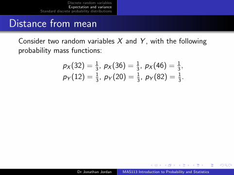
Consider two random variables X and Y , with the followingprobability mass functions:
pX (32) = 13, pX (36) = 1
3, pX (46) = 1
3,
pY (12) = 13, pY (20) = 1
3, pY (82) = 1
3.
Then
E (X ) = 32× 1
3+ 36× 1
3+ 46× 1
3= 38,
E (Y ) = 12× 1
3+ 20× 1
3+ 82× 1
3= 38.
Both X and Y have the same expected value, but forwhatever values of X and Y we observe, X will be closer toE (X ) than Y will be to E (Y ).
Dr Jonathan Jordan MAS113 Introduction to Probability and Statistics
Discrete random variablesExpectation and variance
Standard discrete probability distributions
Distance from mean
Consider two random variables X and Y , with the followingprobability mass functions:
pX (32) = 13, pX (36) = 1
3, pX (46) = 1
3,
pY (12) = 13, pY (20) = 1
3, pY (82) = 1
3.
Then
E (X ) = 32× 1
3+ 36× 1
3+ 46× 1
3= 38,
E (Y ) = 12× 1
3+ 20× 1
3+ 82× 1
3= 38.
Both X and Y have the same expected value, but forwhatever values of X and Y we observe, X will be closer toE (X ) than Y will be to E (Y ).
Dr Jonathan Jordan MAS113 Introduction to Probability and Statistics

Discrete random variablesExpectation and variance
Standard discrete probability distributions
Definition
We use the concept of variance to describe how close arandom variable is likely to be to its expected value.
Definition
The variance Var(X ) of a discrete random variable X isdefined as
Var(X ) : = E[{X − E (X )}2
]= E{(X − µX )2}
=∑x∈RX
(x − µX )2pX (x).
We denote the variance by σ2X :
σ2X := Var(X ).
Dr Jonathan Jordan MAS113 Introduction to Probability and Statistics

Discrete random variablesExpectation and variance
Standard discrete probability distributions
Why squared?
If you are wondering why the variance is defined asE [{X − E (X )}2] rather than E{X − E (X )}, the latterexpression will not tell us anything useful about X :
Theorem
(The expected difference between a random variable and itsmean)
E{X − E (X )} = 0,
for any random variable X .
Dr Jonathan Jordan MAS113 Introduction to Probability and Statistics

Discrete random variablesExpectation and variance
Standard discrete probability distributions
Standard deviation
As the variance is defined as an expected squared difference,the variance will be expressed in units that are the square ofthe units of X .
If we want a measure of spread that is in the same units as X ,we take the square root of the variance.
Definition
The standard deviation of a random variable X , denoted byσX , is the square root of the variance of X .
σX :=√
Var(X ).
Dr Jonathan Jordan MAS113 Introduction to Probability and Statistics

Discrete random variablesExpectation and variance
Standard discrete probability distributions
The variance identity
The following result is useful for calculating variances:
Theorem
Var(X ) = E (X 2)− E (X )2,
Dr Jonathan Jordan MAS113 Introduction to Probability and Statistics

Discrete random variablesExpectation and variance
Standard discrete probability distributions
The variance identity
The following result is useful for calculating variances:
Theorem
Var(X ) = E (X 2)− E (X )2,
Dr Jonathan Jordan MAS113 Introduction to Probability and Statistics

Discrete random variablesExpectation and variance
Standard discrete probability distributions
Calculating the variance
To calculate a variance, if we already have E (X ), we just needto calculate E (X 2).
(Alternatively, if we know the mean and variance, this gives usa quick way of calculating E (X 2)).
Note that as long as Var(X ) > 0 we can see that
E (X 2) 6= E (X )2.
Dr Jonathan Jordan MAS113 Introduction to Probability and Statistics

Discrete random variablesExpectation and variance
Standard discrete probability distributions
Example
Example
Let X be the random variable defined in the roulette example,with E (X ) = −1/37. What is Var(X )?
Dr Jonathan Jordan MAS113 Introduction to Probability and Statistics

Discrete random variablesExpectation and variance
Standard discrete probability distributions
The expectation and variance of aX + b
Theorem
Let X be a random variable, and a and b be any twoconstants. Then
E (aX + b) = aE (X ) + b,
Var(aX + b) = a2 Var(X ).
Dr Jonathan Jordan MAS113 Introduction to Probability and Statistics

Discrete random variablesExpectation and variance
Standard discrete probability distributions
Special cases
If we set a = 0, then we can see that for any constant b,
E (b) = b,
Var(b) = 0.
Dr Jonathan Jordan MAS113 Introduction to Probability and Statistics

Discrete random variablesExpectation and variance
Standard discrete probability distributions
Expectation of a sum
It is often useful to consider expectations of sums of randomvariables:
Theorem
Given any two random variables X and Y
E (X + Y ) = E (X ) + E (Y ).
Dr Jonathan Jordan MAS113 Introduction to Probability and Statistics

Discrete random variablesExpectation and variance
Standard discrete probability distributions
Expectation of a product
We might hope that the same was true for variance, so thatthe variance of X + Y was the sum of the variances of X andY .
This is not true in general, but it is true when X and Y areindependent. To prove this we will first of all prove animportant result about the expectation of a product ofindependent random variables.
Theorem
For any two random variables X and Y which are independent,
E (XY ) = E (X )E (Y ).
Dr Jonathan Jordan MAS113 Introduction to Probability and Statistics

Discrete random variablesExpectation and variance
Standard discrete probability distributions
Variance of independent sum
Corollary
For any two random variables X and Y which are independent,
Var(X + Y ) = Var(X ) + Var(Y ).
Dr Jonathan Jordan MAS113 Introduction to Probability and Statistics

Discrete random variablesExpectation and variance
Standard discrete probability distributions
Example
Example
Let X and Y be independent random variables withVar(X ) = 9 and Var(Y ) = 16. What is Var(X − Y )?
Dr Jonathan Jordan MAS113 Introduction to Probability and Statistics

Discrete random variablesExpectation and variance
Standard discrete probability distributions
Standard probability distributions
We now consider some standard probability distributions fordiscrete random variables, that can be used in a variety ofdifferent applications.
By “distribution”, we mean a particular choice of probabilitymass function, which may be specified in terms of someparameters.
Dr Jonathan Jordan MAS113 Introduction to Probability and Statistics

Discrete random variablesExpectation and variance
Standard discrete probability distributions
The Bernoulli distribution
A Bernoulli random variable X can take one of two values: 0and 1.
Examples of ‘experiments’ that we might describe using aBernoulli random variable are
a patient is given a drug, and the drug either ‘works’:X = 1, or does not: X = 0;
a tennis player either wins a match: X = 1, or loses:X = 0;
in one year, a house is either burgled: X = 1, or not:X = 0.
Dr Jonathan Jordan MAS113 Introduction to Probability and Statistics

Discrete random variablesExpectation and variance
Standard discrete probability distributions
Definition
Definition
If a random variable X has a Bernoulli distribution, then itsprobability mass function is
pX (1) = p,
pX (0) = 1− p,
and pX (x) = 0 otherwise, with 0 ≤ p ≤ 1.We write
X ∼ Bernoulli(p),
to mean “X has a Bernoulli distribution with parameter p’(the probability that X = 1)”.
Dr Jonathan Jordan MAS113 Introduction to Probability and Statistics

Discrete random variablesExpectation and variance
Standard discrete probability distributions
Definition
Definition
If a random variable X has a Bernoulli distribution, then itsprobability mass function is
pX (1) = p,
pX (0) = 1− p,
and pX (x) = 0 otherwise, with 0 ≤ p ≤ 1.
We writeX ∼ Bernoulli(p),
to mean “X has a Bernoulli distribution with parameter p’(the probability that X = 1)”.
Dr Jonathan Jordan MAS113 Introduction to Probability and Statistics

Discrete random variablesExpectation and variance
Standard discrete probability distributions
Definition
Definition
If a random variable X has a Bernoulli distribution, then itsprobability mass function is
pX (1) = p,
pX (0) = 1− p,
and pX (x) = 0 otherwise, with 0 ≤ p ≤ 1.We write
X ∼ Bernoulli(p),
to mean “X has a Bernoulli distribution with parameter p’(the probability that X = 1)”.
Dr Jonathan Jordan MAS113 Introduction to Probability and Statistics

Discrete random variablesExpectation and variance
Standard discrete probability distributions
Definition
Definition
If a random variable X has a Bernoulli distribution, then itsprobability mass function is
pX (1) = p,
pX (0) = 1− p,
and pX (x) = 0 otherwise, with 0 ≤ p ≤ 1.We write
X ∼ Bernoulli(p),
to mean “X has a Bernoulli distribution with parameter p’(the probability that X = 1)”.
Dr Jonathan Jordan MAS113 Introduction to Probability and Statistics

Discrete random variablesExpectation and variance
Standard discrete probability distributions
Mean and variance
Theorem
(Expectation and variance of a Bernoulli random variable)For the expectation of a Bernoulli random variableX ∼ Bernoulli(p), we have
E (X ) = p,
Var(X ) = p(1− p).
Dr Jonathan Jordan MAS113 Introduction to Probability and Statistics

Discrete random variablesExpectation and variance
Standard discrete probability distributions
The binomial distribution
Consider the following situations:
100 patients are given a drug. Each patient either‘responds’ to the drug, or does not. X is the number ofpatients that respond to the drug.
in a crime survey, 1000 people are selected at random,and asked whether they have been burgled in the lastyear. X is the number of people who respond ‘yes’.
in a quality control procedure, 20 items are selected atrandom, and tested to see whether they are faulty. X isthe number of faulty items.
Dr Jonathan Jordan MAS113 Introduction to Probability and Statistics
Discrete random variablesExpectation and variance
Standard discrete probability distributions
Bernoulli trials
In each case we have a fixed number of “trials”, each of whichcan have two possible outcomes (often called “success” and“failure”).
(Each trial can be considered an example of a Bernoullidistribution, with “success” corresponding to 1 and “failure”to 0, so they are often referred to as Bernoulli trials.)
In each of these situations it is reasonable to assume that theprobability of a “success”, which we will call p, is constantfrom from one trial to the next, and that the trials areindependent.
In each case we are counting the total number of successes.
Dr Jonathan Jordan MAS113 Introduction to Probability and Statistics

Discrete random variablesExpectation and variance
Standard discrete probability distributions
Bernoulli trials
In each case we have a fixed number of “trials”, each of whichcan have two possible outcomes (often called “success” and“failure”).
(Each trial can be considered an example of a Bernoullidistribution, with “success” corresponding to 1 and “failure”to 0, so they are often referred to as Bernoulli trials.)
In each of these situations it is reasonable to assume that theprobability of a “success”, which we will call p, is constantfrom from one trial to the next, and that the trials areindependent.
In each case we are counting the total number of successes.Dr Jonathan Jordan MAS113 Introduction to Probability and Statistics

Discrete random variablesExpectation and variance
Standard discrete probability distributions
n = 2
To think about the form of the probability mass function of X ,consider the case n = 2. The possible outcomes are
(on board)
Consider calculating pX (1).
We are not interested in which trials are successes, only thetotal number of successes
There are two ways of achieving one success in total, and foreach of these possibilities, the corresponding probability isp(1− p), so we have pX (1) = 2p(1− p).
Dr Jonathan Jordan MAS113 Introduction to Probability and Statistics

Discrete random variablesExpectation and variance
Standard discrete probability distributions
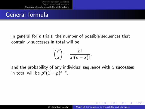
General formula
In general for n trials, the number of possible sequences thatcontain x successes in total will be
(n
x
)=
n!
x!(n − x)!,
and the probability of any individual sequence with x successesin total will be px(1− p)n−x .
So we will have pX (x) =(nx
)px(1− p)n−x .
Dr Jonathan Jordan MAS113 Introduction to Probability and Statistics

Discrete random variablesExpectation and variance
Standard discrete probability distributions
General formula
In general for n trials, the number of possible sequences thatcontain x successes in total will be(
n
x
)=
n!
x!(n − x)!,
and the probability of any individual sequence with x successesin total will be px(1− p)n−x .
So we will have pX (x) =(nx
)px(1− p)n−x .
Dr Jonathan Jordan MAS113 Introduction to Probability and Statistics
Discrete random variablesExpectation and variance
Standard discrete probability distributions
Definition
Motivated by this, we make the following definition:
Definition
If a random variable X has a binomial distribution, withparameters n (the number of trials) and p (the probability ofsuccess in each trial), then the probability mass function of Xis given by
pX (x) =n!
x!(n − x)!px(1− p)n−x ,
for x ∈ RX = {0, 1, 2, . . . , n}, and 0 otherwise.We write X ∼ Bin(n, p), to mean “X has a binomialdistribution with parameters n (the number of trials) and p(the probability of success in each trial)”.
Dr Jonathan Jordan MAS113 Introduction to Probability and Statistics

Discrete random variablesExpectation and variance
Standard discrete probability distributions
Definition
Motivated by this, we make the following definition:
Definition
If a random variable X has a binomial distribution, withparameters n (the number of trials) and p (the probability ofsuccess in each trial), then the probability mass function of Xis given by
pX (x) =n!
x!(n − x)!px(1− p)n−x ,
for x ∈ RX = {0, 1, 2, . . . , n}, and 0 otherwise.
We write X ∼ Bin(n, p), to mean “X has a binomialdistribution with parameters n (the number of trials) and p(the probability of success in each trial)”.
Dr Jonathan Jordan MAS113 Introduction to Probability and Statistics

Discrete random variablesExpectation and variance
Standard discrete probability distributions
Definition
Motivated by this, we make the following definition:
Definition
If a random variable X has a binomial distribution, withparameters n (the number of trials) and p (the probability ofsuccess in each trial), then the probability mass function of Xis given by
pX (x) =n!
x!(n − x)!px(1− p)n−x ,
for x ∈ RX = {0, 1, 2, . . . , n}, and 0 otherwise.We write X ∼ Bin(n, p),
to mean “X has a binomialdistribution with parameters n (the number of trials) and p(the probability of success in each trial)”.
Dr Jonathan Jordan MAS113 Introduction to Probability and Statistics

Discrete random variablesExpectation and variance
Standard discrete probability distributions
Definition
Motivated by this, we make the following definition:
Definition
If a random variable X has a binomial distribution, withparameters n (the number of trials) and p (the probability ofsuccess in each trial), then the probability mass function of Xis given by
pX (x) =n!
x!(n − x)!px(1− p)n−x ,
for x ∈ RX = {0, 1, 2, . . . , n}, and 0 otherwise.We write X ∼ Bin(n, p), to mean “X has a binomialdistribution with parameters n (the number of trials) and p(the probability of success in each trial)”.
Dr Jonathan Jordan MAS113 Introduction to Probability and Statistics

Discrete random variablesExpectation and variance
Standard discrete probability distributions
Link to binomial theorem
Note that the binomial theorem confirms that the binomialprobability mass function is valid (ie it sums to 1):
It tells us that
(a + b)n =n∑
x=0
(n
x
)axbn−x .
and if we now choose a = p and b = 1− p, we have
n∑x=0
pX (x) =n∑
x=0
(n
x
)px(1− p)n−x = (p + (1− p))n = 1,
as we should have.
Dr Jonathan Jordan MAS113 Introduction to Probability and Statistics

Discrete random variablesExpectation and variance
Standard discrete probability distributions
Link to binomial theorem
Note that the binomial theorem confirms that the binomialprobability mass function is valid (ie it sums to 1):
It tells us that
(a + b)n =n∑
x=0
(n
x
)axbn−x .
and if we now choose a = p and b = 1− p, we have
n∑x=0
pX (x) =n∑
x=0
(n
x
)px(1− p)n−x = (p + (1− p))n = 1,
as we should have.Dr Jonathan Jordan MAS113 Introduction to Probability and Statistics

Discrete random variablesExpectation and variance
Standard discrete probability distributions
Mean and variance
Theorem
(Expectation and variance of a binomial random variable)For X ∼ Bin(n, p) we have
E (X ) = np
Var(X ) = np(1− p).
Dr Jonathan Jordan MAS113 Introduction to Probability and Statistics

Discrete random variablesExpectation and variance
Standard discrete probability distributions
Mean and variance
Theorem
(Expectation and variance of a binomial random variable)For X ∼ Bin(n, p) we have
E (X ) = np
Var(X ) = np(1− p).
Dr Jonathan Jordan MAS113 Introduction to Probability and Statistics
Discrete random variablesExpectation and variance
Standard discrete probability distributions
Proportion of successes
As well as being interested in the total number of ‘successes’X , we may also be interested in the proportion of success X/n.
We have
E
(X
n
)= p,
Var
(X
n
)=
p(1− p)
n.
What do you think will happen to X/n as n→∞?
Dr Jonathan Jordan MAS113 Introduction to Probability and Statistics
Discrete random variablesExpectation and variance
Standard discrete probability distributions
The cumulative distribution function
The cumulative distribution function is given by
FX (x) = P(X ≤ x) =x∑
a=0
pX (a)
=x∑
a=0
n!
a!(n − a)!pa(1− p)n−a.
We cannot simplify this expression, and so calculating thec.d.f. by hand can be tedious.
Fortunately, we can do this and other calculations related tothe binomial distribution very easily in R.
Dr Jonathan Jordan MAS113 Introduction to Probability and Statistics

Discrete random variablesExpectation and variance
Standard discrete probability distributions
The binomial distribution in R
As with most standard distributions in R, there are commandsfor calculating the p.m.f., c.d.f., quantile function, and forrandomly sampling from the distribution.
Dr Jonathan Jordan MAS113 Introduction to Probability and Statistics

Discrete random variablesExpectation and variance
Standard discrete probability distributions
The binomial distribution: examples
Example
A company claims that, for a particular product, 8 out of 10people prefer their brand A over a rival’s brand B .
You randomly sample 50 people, and ask them whether theyprefer brand A to brand B .Let X be the number of people who choose brand A.
Dr Jonathan Jordan MAS113 Introduction to Probability and Statistics

Discrete random variablesExpectation and variance
Standard discrete probability distributions
The binomial distribution: examples
Example
A company claims that, for a particular product, 8 out of 10people prefer their brand A over a rival’s brand B .You randomly sample 50 people, and ask them whether theyprefer brand A to brand B .
Let X be the number of people who choose brand A.
Dr Jonathan Jordan MAS113 Introduction to Probability and Statistics

Discrete random variablesExpectation and variance
Standard discrete probability distributions
The binomial distribution: examples
Example
A company claims that, for a particular product, 8 out of 10people prefer their brand A over a rival’s brand B .You randomly sample 50 people, and ask them whether theyprefer brand A to brand B .Let X be the number of people who choose brand A.
Dr Jonathan Jordan MAS113 Introduction to Probability and Statistics

Discrete random variablesExpectation and variance
Standard discrete probability distributions
The binomial distribution: examples
Example
If the company is right,
1 What are the expectation and variance of X ?
2 What is the probability that X = 40?
3 What is the probability that X ≤ 30?
4 What is the probability that X ≥ 45?
Dr Jonathan Jordan MAS113 Introduction to Probability and Statistics
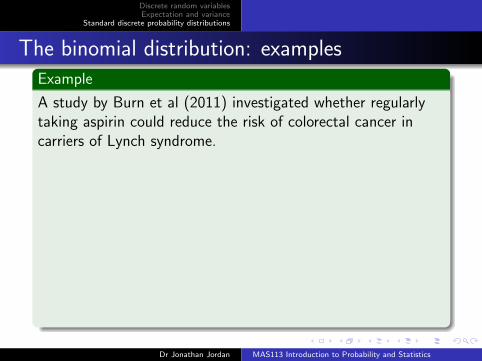
Discrete random variablesExpectation and variance
Standard discrete probability distributions
The binomial distribution: examplesExample
A study by Burn et al (2011) investigated whether regularlytaking aspirin could reduce the risk of colorectal cancer incarriers of Lynch syndrome.
In a control group, 434 participants regularly took a placebo,and over the period of the study, 30 members of the controlgroup developed primary colorectal cancers.In the treatment group, 427 participants regularly took aspirin,and 18 members developed primary colorectal cancers.Let X be the number of participants in the treatment groupwho developed primary colorectal cancers.Suppose the probability of a participant developing a cancerwas 30/434, regardless of which group the participant was in.
Dr Jonathan Jordan MAS113 Introduction to Probability and Statistics

Discrete random variablesExpectation and variance
Standard discrete probability distributions
The binomial distribution: examplesExample
A study by Burn et al (2011) investigated whether regularlytaking aspirin could reduce the risk of colorectal cancer incarriers of Lynch syndrome.In a control group, 434 participants regularly took a placebo,and over the period of the study, 30 members of the controlgroup developed primary colorectal cancers.
In the treatment group, 427 participants regularly took aspirin,and 18 members developed primary colorectal cancers.Let X be the number of participants in the treatment groupwho developed primary colorectal cancers.Suppose the probability of a participant developing a cancerwas 30/434, regardless of which group the participant was in.
Dr Jonathan Jordan MAS113 Introduction to Probability and Statistics
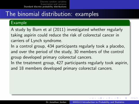
Discrete random variablesExpectation and variance
Standard discrete probability distributions
The binomial distribution: examplesExample
A study by Burn et al (2011) investigated whether regularlytaking aspirin could reduce the risk of colorectal cancer incarriers of Lynch syndrome.In a control group, 434 participants regularly took a placebo,and over the period of the study, 30 members of the controlgroup developed primary colorectal cancers.In the treatment group, 427 participants regularly took aspirin,and 18 members developed primary colorectal cancers.
Let X be the number of participants in the treatment groupwho developed primary colorectal cancers.Suppose the probability of a participant developing a cancerwas 30/434, regardless of which group the participant was in.
Dr Jonathan Jordan MAS113 Introduction to Probability and Statistics

Discrete random variablesExpectation and variance
Standard discrete probability distributions
The binomial distribution: examplesExample
A study by Burn et al (2011) investigated whether regularlytaking aspirin could reduce the risk of colorectal cancer incarriers of Lynch syndrome.In a control group, 434 participants regularly took a placebo,and over the period of the study, 30 members of the controlgroup developed primary colorectal cancers.In the treatment group, 427 participants regularly took aspirin,and 18 members developed primary colorectal cancers.Let X be the number of participants in the treatment groupwho developed primary colorectal cancers.
Suppose the probability of a participant developing a cancerwas 30/434, regardless of which group the participant was in.
Dr Jonathan Jordan MAS113 Introduction to Probability and Statistics

Discrete random variablesExpectation and variance
Standard discrete probability distributions
The binomial distribution: examplesExample
A study by Burn et al (2011) investigated whether regularlytaking aspirin could reduce the risk of colorectal cancer incarriers of Lynch syndrome.In a control group, 434 participants regularly took a placebo,and over the period of the study, 30 members of the controlgroup developed primary colorectal cancers.In the treatment group, 427 participants regularly took aspirin,and 18 members developed primary colorectal cancers.Let X be the number of participants in the treatment groupwho developed primary colorectal cancers.Suppose the probability of a participant developing a cancerwas 30/434, regardless of which group the participant was in.
Dr Jonathan Jordan MAS113 Introduction to Probability and Statistics

Discrete random variablesExpectation and variance
Standard discrete probability distributions
The binomial distribution: examples
Example
1 Calculate the probability that no more than 18participants in the treatment group develop primarycolorectal cancers.
2 Find the 2.5th and 97.5th percentiles of X .
Note that formal methods for testing whether there is a“significant” difference between the two groups will be coveredin Semester 2.
Dr Jonathan Jordan MAS113 Introduction to Probability and Statistics

Discrete random variablesExpectation and variance
Standard discrete probability distributions
The Poisson distribution
The Poisson distribution is used to represent count data: thenumber of times an event occurs in some finite interval in timeor space.
Some situations that we might model using a Poissondistribution are as follows.
The number of arrivals at an Accident & Emergency wardin one night;
the number of burglaries in a city in a year;
the number of goals scored by a team in a football match;
the number of leaks in 1km section of water pipe.
Dr Jonathan Jordan MAS113 Introduction to Probability and Statistics
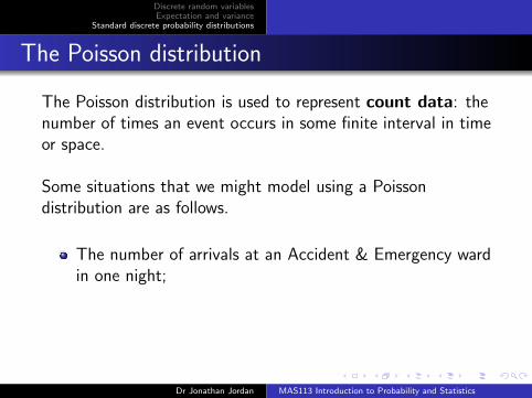
Discrete random variablesExpectation and variance
Standard discrete probability distributions
The Poisson distribution
The Poisson distribution is used to represent count data: thenumber of times an event occurs in some finite interval in timeor space.
Some situations that we might model using a Poissondistribution are as follows.
The number of arrivals at an Accident & Emergency wardin one night;
the number of burglaries in a city in a year;
the number of goals scored by a team in a football match;
the number of leaks in 1km section of water pipe.
Dr Jonathan Jordan MAS113 Introduction to Probability and Statistics
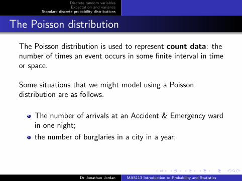
Discrete random variablesExpectation and variance
Standard discrete probability distributions
The Poisson distribution
The Poisson distribution is used to represent count data: thenumber of times an event occurs in some finite interval in timeor space.
Some situations that we might model using a Poissondistribution are as follows.
The number of arrivals at an Accident & Emergency wardin one night;
the number of burglaries in a city in a year;
the number of goals scored by a team in a football match;
the number of leaks in 1km section of water pipe.
Dr Jonathan Jordan MAS113 Introduction to Probability and Statistics

Discrete random variablesExpectation and variance
Standard discrete probability distributions
Motivation
We can motivate the form of the Poisson distribution asfollows.
Consider the third example, assume that we expect the teamto score about λ goals (for some λ) and imagine dividing thematch up into n short time intervals, where n is some arbitrarybut large number.
(E.g. n could be 90 and each of the intervals one minute long.)
Dr Jonathan Jordan MAS113 Introduction to Probability and Statistics

Discrete random variablesExpectation and variance
Standard discrete probability distributions
Motivation continued
Assume that in each of these time intervals the probability ofthe team scoring one goal is p, independently of the otherintervals, and that the probability of them scoring more thanone goal in an interval is “negligible”.
Under these assumptions, the number of goals scored has aBin(n, p) distribution.
That the expectation of a Bin(n, p) random variable is npsuggests that we should now take p = λ/n.
Because we set n to be large, this suggests we should considerthe behaviour of Bin(n, λ/n) for large n.
Dr Jonathan Jordan MAS113 Introduction to Probability and Statistics

Discrete random variablesExpectation and variance
Standard discrete probability distributions
Limit of Binomials
Theorem
Consider X ∼ Bin(n, λ/n), and suppose that n→∞.
Then, as n→∞
pX (x)→ e−λλx
x!.
Dr Jonathan Jordan MAS113 Introduction to Probability and Statistics

Discrete random variablesExpectation and variance
Standard discrete probability distributions
Limit of Binomials
Theorem
Consider X ∼ Bin(n, λ/n), and suppose that n→∞.Then, as n→∞
pX (x)→ e−λλx
x!.
Dr Jonathan Jordan MAS113 Introduction to Probability and Statistics
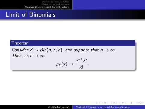
Discrete random variablesExpectation and variance
Standard discrete probability distributions
Limit of Binomials
Theorem
Consider X ∼ Bin(n, λ/n), and suppose that n→∞.Then, as n→∞
pX (x)→ e−λλx
x!.
Dr Jonathan Jordan MAS113 Introduction to Probability and Statistics
Discrete random variablesExpectation and variance
Standard discrete probability distributions
Definition
Motivated by this result, we make the following definition:
Definition
If a random variable X has a Poisson distribution, withparameter λ > 0, then its probability mass function is given by
pX (x) = P(X = x) =e−λλx
x!,
for x ∈ N0 and 0 otherwise.We write X ∼ Poisson(λ),to mean “X has a Poisson distribution with rate parameter λ”.
Dr Jonathan Jordan MAS113 Introduction to Probability and Statistics
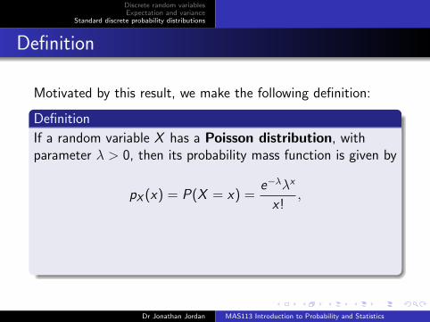

Discrete random variablesExpectation and variance
Standard discrete probability distributions
Definition
Motivated by this result, we make the following definition:
Definition
If a random variable X has a Poisson distribution, withparameter λ > 0, then its probability mass function is given by
pX (x) = P(X = x) =e−λλx
x!,
for x ∈ N0 and 0 otherwise.
We write X ∼ Poisson(λ),to mean “X has a Poisson distribution with rate parameter λ”.
Dr Jonathan Jordan MAS113 Introduction to Probability and Statistics

Discrete random variablesExpectation and variance
Standard discrete probability distributions
Definition
Motivated by this result, we make the following definition:
Definition
If a random variable X has a Poisson distribution, withparameter λ > 0, then its probability mass function is given by
pX (x) = P(X = x) =e−λλx
x!,
for x ∈ N0 and 0 otherwise.We write X ∼ Poisson(λ),to mean “X has a Poisson distribution with rate parameter λ”.
Dr Jonathan Jordan MAS113 Introduction to Probability and Statistics

Discrete random variablesExpectation and variance
Standard discrete probability distributions
Parameter
The Poisson distribution has a single parameter λ, known asthe rate parameter.
Shortly, we will show that E (X ) = λ, so you can interpret λ asthe expected number of times the event will occur.
Dr Jonathan Jordan MAS113 Introduction to Probability and Statistics

Discrete random variablesExpectation and variance
Standard discrete probability distributions
Sum to 1, mean and variance
Theorem
(Poisson random variable: valid p.m.f., expectation andvariance)
1 The Poisson probability mass function is a validprobability mass function.
2 If X ∼ Poisson(λ) then
E (X ) = Var(X ) = λ.
Dr Jonathan Jordan MAS113 Introduction to Probability and Statistics
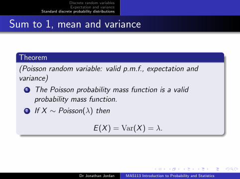
Discrete random variablesExpectation and variance
Standard discrete probability distributions
Sum to 1, mean and variance
Theorem
(Poisson random variable: valid p.m.f., expectation andvariance)
1 The Poisson probability mass function is a validprobability mass function.
2 If X ∼ Poisson(λ) then
E (X ) = Var(X ) = λ.
Dr Jonathan Jordan MAS113 Introduction to Probability and Statistics

Discrete random variablesExpectation and variance
Standard discrete probability distributions
The cumulative distribution function
The cumulative distribution function is given by
FX (x) = P(X ≤ x) =x∑
a=0
pX (a)
=x∑
a=0
e−λλa
a!.
As with the binomial distribution, this is tedious to calculateby hand, but easy to calculate using R.
Dr Jonathan Jordan MAS113 Introduction to Probability and Statistics

Discrete random variablesExpectation and variance
Standard discrete probability distributions
The Poisson distribution in R
dpois(x,lambda) for p.m.f.
pppois(x,lambda) for c.d.f.
qpois(alpha,lambda) for quantile function
rpois(m,lambda) for m random observations
Dr Jonathan Jordan MAS113 Introduction to Probability and Statistics
Discrete random variablesExpectation and variance
Standard discrete probability distributions
The Poisson distribution: examples
Example
Suppose X , the number of accidents at a road junction in oneyear has a Poisson distribution with rate parameter 5.
1 What are the expectation and variance of X ?
2 What is the probability that X = 0?
3 What is the probability that X ≤ 5?
4 What is the probability that X ≥ 10?
Dr Jonathan Jordan MAS113 Introduction to Probability and Statistics
Discrete random variablesExpectation and variance
Standard discrete probability distributions
Approximating the Binomial
Note that Theorem 14 suggests that for large n and small p,the Bin(n, p) distribution can be well approximated by thePoisson(np) distribution.
Example
An article published on the BBC news website reported“three-fold variation” in UK bowel cancer death rates. Theaverage death rate from bowel cancer across the UK isreported as 17.6 per 100,000.By considering 100 ‘regions’ each with the same populationsize of 100,000, how much variation could be due to chancealone?
Dr Jonathan Jordan MAS113 Introduction to Probability and Statistics

Discrete random variablesExpectation and variance
Standard discrete probability distributions
Approximating the Binomial
Note that Theorem 14 suggests that for large n and small p,the Bin(n, p) distribution can be well approximated by thePoisson(np) distribution.
Example
An article published on the BBC news website reported“three-fold variation” in UK bowel cancer death rates. Theaverage death rate from bowel cancer across the UK isreported as 17.6 per 100,000.
By considering 100 ‘regions’ each with the same populationsize of 100,000, how much variation could be due to chancealone?
Dr Jonathan Jordan MAS113 Introduction to Probability and Statistics

Discrete random variablesExpectation and variance
Standard discrete probability distributions
Approximating the Binomial
Note that Theorem 14 suggests that for large n and small p,the Bin(n, p) distribution can be well approximated by thePoisson(np) distribution.
Example
An article published on the BBC news website reported“three-fold variation” in UK bowel cancer death rates. Theaverage death rate from bowel cancer across the UK isreported as 17.6 per 100,000.By considering 100 ‘regions’ each with the same populationsize of 100,000, how much variation could be due to chancealone?
Dr Jonathan Jordan MAS113 Introduction to Probability and Statistics

Discrete random variablesExpectation and variance
Standard discrete probability distributions
The geometric distribution
Consider the following situations:
Throwing darts at a dartboard until the bull’s eye is hit;
Buying a national lottery ticket each week until thejackpot is won.
As with the Binomial examples, these involve a sequence ofBernoulli trials, each of which a ‘success’, with probability p,or a ‘failure’, with probability 1− p, but now there is no fixednumber of trials; rather, we repeat the trials until we obtain asuccess.
Dr Jonathan Jordan MAS113 Introduction to Probability and Statistics

Discrete random variablesExpectation and variance
Standard discrete probability distributions
Definition
A geometric random variable X is the number of the trial inwhich the first success is observed.
Definition
If a random variable X has a geometric distribution, withparameter p (the probability of a success in any single trial),then the probability mass function of X is given by
pX (x) = (1− p)x−1p,
for x ∈ N and 0 otherwise.We write X ∼ Geometric(p).
Dr Jonathan Jordan MAS113 Introduction to Probability and Statistics

Discrete random variablesExpectation and variance
Standard discrete probability distributions
Definition
A geometric random variable X is the number of the trial inwhich the first success is observed.
Definition
If a random variable X has a geometric distribution, withparameter p (the probability of a success in any single trial),then the probability mass function of X is given by
pX (x) = (1− p)x−1p,
for x ∈ N and 0 otherwise.
We write X ∼ Geometric(p).
Dr Jonathan Jordan MAS113 Introduction to Probability and Statistics

Discrete random variablesExpectation and variance
Standard discrete probability distributions
Definition
A geometric random variable X is the number of the trial inwhich the first success is observed.
Definition
If a random variable X has a geometric distribution, withparameter p (the probability of a success in any single trial),then the probability mass function of X is given by
pX (x) = (1− p)x−1p,
for x ∈ N and 0 otherwise.We write X ∼ Geometric(p).
Dr Jonathan Jordan MAS113 Introduction to Probability and Statistics

Discrete random variablesExpectation and variance
Standard discrete probability distributions
C.D.F
Theorem
(Cumulative distribution function of a geometric randomvariable)If X ∼ Geometric(p) and x is a non-negative integer then
FX (x) = 1− (1− p)x .
Dr Jonathan Jordan MAS113 Introduction to Probability and Statistics
Discrete random variablesExpectation and variance
Standard discrete probability distributions
Valid distribution
Note that as x →∞, (1− p)x → 0, so that
∞∑x=1
pX (x) = FX (∞) = 1,
confirming that the probability mass function is valid.
Dr Jonathan Jordan MAS113 Introduction to Probability and Statistics

Discrete random variablesExpectation and variance
Standard discrete probability distributions
Mean and variance
Theorem
(Expectation and variance of a geometric random variable)If X ∼ Geometric(p) then
E (X ) =1
p
Var(X ) =1− p
p2.
Dr Jonathan Jordan MAS113 Introduction to Probability and Statistics

Discrete random variablesExpectation and variance
Standard discrete probability distributions
Example
Example
In section 5.1, we calculated the probability of winning theNational Lottery jackpot with a single ticket is p = 1
45057474.
Suppose I buy one ticket per week. Let X be the week numberin which I first win the jackpot.
1 What are the expectation and variance of X ?
2 What is the probability that I don’t win at any time in thenext 50 years?
Dr Jonathan Jordan MAS113 Introduction to Probability and Statistics