Embed Size (px)
Citation preview

,AD-A125 047 FEARS USER'S MANUAL FOR UNIVAC ii88(U) MARYLAND UNIV i/iCOLLEGE PARK LAB FOR NUMERICAL ANALYSIS
MESZTENYI ET AL. OCT 82 BN-99i N8614-77-C-923
UNCLASSIFIED F/G 9/2 N
Eh1h h 10 1 0 iE

At
Fl
t
~ 4 .- - 'V
-
1
/
IM
)~. -I
1.1 t -' . 7\t\ -I I -- - I- -~
flU a a
E±~EUJ~.EJ~2.
j . F
I.U
MICROCOPf RESOLUTION TEST CHARTNArIOtGAL SUUEAU OF SrANOANOS-1W3-AI >~ -'
N
.1~
- * * 'r-------.g..--r. -**.--~ ~.,* -
~~ ~*d:~ '. ~ **. . . . -. . -
* *~* *~ F*~ F

INSTITUT; f:OR PI-JYSICAL SCICFNCI (7AND TgCP1NOLOG;Y
Laboratory for Numerical Analysis
Tecbnica3 Note fto. hN-991
IM USER'01 MAUU
!or UNI VAC 110ICag
by 1
C. XaLsztemyi, 1-. Szymczak
CS 83 02 028 048LIJ
Ict' Aber 1982
UNIVC-RSITY OF MARYLAND

Encl (1)
SECURITY CLASSIFICATION Ou THIS PAGEt (Ubu ue= e
REPOT DOCUMETATION PAGE *310U W8UPLTSGFaU
1. REPORT N4UMBER IOV CESUON E RECIPIEMT'S CATALOG Nummi&A
Technical Note BN-991 I44 r V" _ _ _ __ _ _ _ __ _ _ _ _
4. TITLE (an.d Su~hel) L. TYPR OF REPORT A PRID COVEREDFEARS USER'S MANUAL FOR UNIVAC 1100 final-life of the contract
S. PERVORNING OF4G. REPORT NUMBER
7. AUTHN(s) 6. CONTRACT OR GRANT NUMMAR-.
C. Mesztenyi and W1. Sztmczak ONR N00014-7 7-C-0623
9. PERFORMING ORGANIZATION NAME AND ADDRESS 10. PRRA IENTPOJC.ASInstitute for Physical Science & Technology AREAU UMUUER
University of MarylandCollege Park, MD 20742
I I- CONTROLLING OFFICE NAME AND AD0RESS IL. REPORT DATE
Department of the Navy October 1982Office of Naval Research Is. 1110aftErO PAGES
Arlington, VA 22217 7444I. MONITORING AGENCY NAI-Of DNS(I lhtk Cenvel& *m@*e) IILS. CURVITY CLASS. (of 000 utmg
IS. DSTRUTION STATEMENT (of dof. Ree)
Approved for public release: distribution unlimited
17I. WISTRINUTION STATEMENT (*lobh* ebotrat mugeeE i. lek.h 1110100""mukm RM)~w
IS. SUPPLEMENTARY NOTES
IfI
20. AGST RACT (Cntime on revrs .Eds D N.en mesrdd 1~10M, e minuhe* The FEARS program normally takes the problem a descriptive data from the run-* stream. This input data is composed of the Geometry (Chapter 1) and of the
Bilinear/Error matrices (Chapter 2). Alternatively, this data can be read froma "DUIIP-file", which has been generated by a previous execution of FEARS (section3.13). Once the initial data is read, FEARS enters into a command-mode. In the
* command-mode, the user must input a command (with some parameters) instrluctingthe program about the next step to be taken. The available commands are given inChapter 3. This mode allows the user to have complete control over the interatio
DO FOR7 1473 EDITION OP I NOV 65 IS OSSOLETES.'N 010?- LF-014-6601 EUT ASPATOOPWIPAE(mDu

process, step by step, reflecting the research nature of the program. On theother hand, the ITERATE co mand allows the iterations to be automatic. Oncea STOP command is given, the run will be terminated.
Printed output generated by FEARS consists of summary data after eachiteration step. The user also has the option to reprint initial input and/or
detailed information about the solution process during the iteration. Theformats of these printouts are described in Chapter4. In addition, the DUMPcommand generates a dump-file of the data structure which can be used as input,either for FEARS itself, or for various post-processors. The format of this dump-file is described in Section 4.7.
Chapter 5 gives the computer dependent control statements necessaryto run FEARS on the UNIVAC 1100 computer. The program is supplied with adummy subroutine giving zero values for the bilinear matrices E and D ,
(see Section 2.7). If these matrices are coordinate dependent, the user mustsupply the appropriate subroutine replacing the supplied dummy routine. Thispreparation must be performed prior to the use of FEARS.
. . ...
420.K
"C
*1r!
.
a

SFR
USER'S MANIUAL
for UNIVAC 1100
.~ e~:by C. Mesztenyi, W. Szymczak
6 Technical Note No. BN-991
prICSFES 819830
The work was partially supported by ONR Contract N00014-77-C-0623.The computation was partially supported by the Computer Science Center of
'23 the University of Maryland.

t.. Table of Contents - FEARS Userts Manual
Chapter
0. Introduction
1. Geometry Input
1.1 Introduction 2
1.2 Format 4
1.3 Description of the Format 5
2. Bilinear and Error Matrices Input
2.1 Introduction 8
2.2 Variational Form 8
2.3 Error Norms 9
2.4 General Format 9
2.5 Description of the Bilinear and Error Matrices 10
2.6 Line Integration Boundary Conditions 14
2.7 Subroutines for the Functions E(X,Y), D(X,Y) 16
3. User Commands and Strategy
3.1 Introduction-Overview of Strategies 18
3.2 PRINT Command 21
3.3 REPORT Command / 23
7Accession For 233.4 SUBDIVIDE Command
NTSGRA&I
3.5 DOMAIN Command rl T TABP 24
3.6 LONG Command J,. -i, i cat _ 25
3.7 SHORT Command .,.... 253.8Ditribution/
3.8 AUTO Command _27
3.9 ERROR Command Dist 3Ai J 29
3.10 DEBUG Command 1- 29
3.11 OUTPUT Command 31

3.12 DUMP Command 31
3.13 RESET Command 31
3.14 ITERATE Command 32
3.15 CHANGE Command 33
3.16 SHEF Command 35
6% 3.17 STOP Command 35
3.18 ERIT Command 35
3.19 MESH Command 36
3.20 INIT Command 36
4. The Output
'P 4.1 Introduction-Global and Local Coordinates 37
4.2 Numbering the Mesh of a 2-D Domain 37
4.3 The PRINT output 39
4.3.1 Printing the Points (0-D Domains) 39
4.3.2 Printing the Lines (1-D Domain) 40
4.3.3 The 2-D Domain Printout 41
4.4 The TIME Breakdown 43
4.5 The REPORT Printout 44
4.6 The OUTPUT Printout 45
4.7 DUMP File Output 46
5. Starting the FEARS Program
5.1 File Assignments 48
5.2 Preparation for Execution 49
5.3 Execution of FEARS 52
A . APPENDIX
A.1 Sample Geometry 55
A.2 Bilinear and Error Matrices
A.2.1 The Matrix A Arising From Elasticity 60
A.2.2 The Error Matrix AE 61

A.2. Th utu Matrix S 6
A24SampleInus6
A3Cmuainof the Threshold Value 67
B. APPENDIX
FEARS Element Postprocessor 70
.. 7

0. Introduction
) The FEARS program normally takes the problem's descriptive data from
the run-stream. This input data is composed of the Geometry t x"
-and of the Bilinear/Error matrices, ii. Alternatively, this data
can be read am a file which has been generated by a previous
execution of FEARSSe 2 Once the initial data is read, FEARS
enters into a command-mode. In the command-mode, the user must input a
command (with some parameters) instructing the program about the next step
to be taken. The available commands are given in Chapter 3. This mode allows
the user to have complete control over the iteration process, step by step,
reflecting the research nature of the program. On the other hand, the
ITERATE command allows the iterations to be automatic. Once a STOP
- command is given, the run will be terminated.
Printed output generated by FEARS consists of summary data after
each iteration step. The user also has the option to reprint initial
input and/or detailed information about the solution process during the
iteration. The formats of these printouts are described in Chapter 4.
In addition, the DUMP command generates a dump-file of the data structure
which can be used as input, either for FEARS itself, or for various post-
processors. The format of this dump-file is described in Section 4.7.
Chapter 5 gives the computer dependent control statements necessary
to run FEARS on the UNIVAC 1100 computer. The program is supplied with a
duy subroutine giving zero values for the bilinear matrices E and D.
Q ts.-Sit -l-- f - If these matrices are coordinate dependent, the user
must supply the appropriate subroutine replacing the supplied dummy routine.
This preparation must be performed prior to the use of FEARS.

Chapter I. Geometry Input
1.1 Introduction - 0-D, 1-D, and 2-D domains
The domain V, on which the problem is to be solved, must be initially
broken up into subdomains. Each subdomain is a generalized quadrilateral,
having 4 corner points and 4 sides, with each side being either a straight
line or an arc of a circle. Since a unit quare will be mapped onto each
of these subdomains, they should not be "degenerate" or "singular". For
example, the angles formed at the vertices should not be too near 0* or
180, the domains should not be nearly triangular, and no overlapping of
the sides is allowed. Thus, it is good practice to avoid subdomains as
shown in Figure 1.1.
Figure 1.1. Subdomains to be avoided.
Figure 1.2 illustrates how a disk, and triaugular and pentagonal
domains may be substructured into generalized quadrilaterals.
,-' -=-
Figure 1.2. Subdomain structuring for a disk, triangular
domain, and pentagonal domain.
2

Because FEARS uses blending functions to map the unit square onto
each generalized quadrilateral (see FEARS Mathematical Description,
Chapter I), domains having boundaries composed of circular arcs are
I represented exactly and are not approximated by isoparametric elements.
Therefore, the approximations of the geometry and the exact solutions
are not mixed, when using FEARS.
The corner points of the subdomains are simply called points or
O-D domains (zero dimensional domains). These are denoted by
V0 k-l2 .... NO.
k
The open line sexments I oinins the points are called lines or l-D domains,
and are denoted
V 1k k-1,2,....Nl.* k
Finally, the open subdomains, each with 4 lines and 4 points forming its
Uboundary, are called 2-D domains, and are denotedV2 k-l,2,...N2.k
For example, the disk can be structured and labeled as in Figure 1.3,
too
-AA
1 3
Figure 1.3. The substructuring and labeli- of Disk.
3

In the geometry input the following information must be supplied:
(i) the number of points, lines, and 2-D domains,
(ii) the global coordinates of the points,
(iii) the end point indices for each line,
(iv) the radius of each line,
(v) the boundary conditions for each line and point,
and (vi) the cornerpoint indices of each 2-D domain.
1.2 Format
The format for the geometry input is as follows:
NO1, X1 9 yl bl" vl Wl
2, x2 , Y2 .b2 " v2 -v2
. points
;o, XNo' YNO' 'NO' vNO" 'NO
Ni1, P1 9 ql 01 9 P1
2, P2, q2, 823 p2
lines
~N1, PN1 qN 19 N' N1
:tN2
191 2 3 4131 1 '1' 1
2, 1 2 3 42, 1 '2 1 ,2 '2 2-D domains
1 2 3 4N2, v N21 'N2' 'N1 'N12
4

1.3. Description of the Format
NO is the number of points (O-D's). The data, i,xiYibi, vi, Wi,
describe the points as follows:
U0i - the index of 0 , i-l,...,N0,
(xiy 1 ) - the x-y global coordinates of D
b i M the boundary condition at DO where
0 -> u1 free, u2 free,
bm 1 > uI fixed, u2 free,b~i
" !.2 => uI free, u2 fixed,
3 > u 1 fixed, u2 fixed ,and
(vi,wi) - the solution value (ulU2) at o. These must be given
even if the boundary condition is free, in which case
any value for v1 ,w may be given.
N1 is the number of lines (l-D's).. The data j, p ,
describe the lines as follows:
J1
i - the index of V J - 1,...
(pj,ql) - the index numbers of the endpoints of the line V0p V0 ,
- 1jB -the boundary conditions of line V, where
0 -> u1 free, u2 free,
1 -> u1 fixed, u2 free,
2 = u1 free, u2 fixed,
"j= 3=> u1 fixed, u2 fixed,
5 => uI linear, u2 free
6g> u1 free, u2 linear
7 -> u1 linear, u2 linear.
p5

If a component ul, or u 2 is fixed or linear, then the same component
must be fixed at the endpoints DO , and Do . Furthermore, if it isqJ iPJ
fixed then the two values given at these endpoints must be identical.
P -/R± is the signed reciprocal of the radius of the arc
segment The orientation determines the sign of the radius as shown
in Figure 1.4.
p j qq
P j = 1/Rd p =-1/R
Figure 1.4. Orientation of the arcs.
N2 is the number of 2-D domains. The 2-D domains are prescribed by
the 4 corner point indices if N2 is not preceded by a minus sign, and by
the 4 boundary line indices if N2 is preceded by a minus sign.
The first input in each line after N2 is k = the index of V2 k=l,...,N2.
When no minus sign precedes N2, 1k' k k V 2 the index numbers of the 42
cornerpoints of D , in the order shown in Figure 1.5.
2
Figure 1.5. Order of the 4 cornerpoint indices for a 2-D domain.
The user should be careful not to change this orientation. For example,
the indices cannot be input in the order as displayed in Figure 1. 6.
" " .- .;.: . ", ' ' ; -"-'.,'- .- .. '-'.;. : "-' .. .-- '..;..." . - ." - .. • .. " ' - •'6.

2°-3
WRONG I
Figure 1.6. Illegal ordering of the 4 cornerpoint indices for a 2-D domain.
1 2 3 4.. When a minus sign precedes N2, k k 2 3 k = the index numbers of the 4
boundary lines of in the order shown in Figure 1.Z.k
'EZ3
Figure 1.7. Order of the 4 boundary line indices for a 2-D domain.
a-7
I',7
t' "'" ,'; ' ,,; _, '.' . . . . . . ..... . ..- **'',* " ', ' : " " """r " -.- * • **' - _* -. . .. . . .. -, .. - .- .. .

Chapter II. Bilinear and Error Matrices Input
£' 2.1. Introduction
In the previous section, it was seen that FEARS works on a substructured
domain, which allows a simple input and a more accurate representation of the
geometry. The substructuring has another advantage, namely, it also allows
for a different set of material properties (bilinear matrices) to be described
on each 2-D domain.
2.2. Variational Form
The variational problem, solvable by FEARS, can be put in the general
form: find U in Ml, such that
N + VdT
AiU V Bi[J [jZ] BiU + VC1Udx dy
Nl T N2 [3aV1 VTExy N1+ E VYU ds- E /1 T D(xy) + vTE~x,y dx dy + E Ji(s)V ds
J=l J =1Vi V2 Dji
1-4 for all V in M2 , where M1 and M are the appropriate finite
dimensional trial and test spaces (see FEARS Mathematical Description).
Here, we have used the notation
U-u 1 U __3z ix
.. u , au , and analogously for L and V.
au2
Also,
A is a 4 x 4 symmetric matrix,
B is a 2 x 4 matrix,
8

CI Is a 2 x 2syimetric matrix
-D (x,y) is a 4 x 1 vector valued function, and
Ei(x,y) is a 2 x 1 vector valued function, for 1 < i < N2
y j is a 2 x 2 symmetric matrix, and
e (s) is a 1 x 2 vector valued function for i < _ N.
2.3 Error Norms
The error is approximated in the norm 1 where*
.-,N2 SU]T j dU
1: dy (2.1)
The value p is a global value which is input before we input the
geometry and bilinear forms. The values pi are to be specified for each
3 2-D domain. Normally p " P2 - " PN2 - p ' which will correspond to a
global L2p estimate. The corresponding L. norm (2.2), is used when pi 0
II~ i2)- sup V2~ T~j~ (2.2)*xy
(AE) is a 4 x 4 matrix, and usually, (AE) - (A) .
2.4 General Format
The format for the input of the bilinear, error, and output matrices is
as follows:
*That 1110111 is a norm and not a seminorm for the error e , followsfrom the fact RXat if titeill 0 0 , the • must be constant. Since theapproximate solution is bilinelh, the exact solution must be bilinear as
*well. Because of quasi-optimality of the finite element solution, e-0
9
4. - .- , ' , ' '.. ,,> ;., -,- - -....*..'. -.-......-. .. ...- .. . ,. .-. ; .. .;. -. .., - -.,*..*

-a -: - - .. ' -a.±a : " .- a . -a .. - a. . . . -..-.. ' /.t .. .-. -. °- . $. . . -.. . -. -.. -. - . . . . .- .- ,
J, uv, k1 , k2 ... , k n (Bilinear and Error
Matrices)
!0j Bj, Yj, Cj
(A)j (if a, 0) (This packet is repeated
(B)~ (if 0~) NB times, J-1. ... 'IM)-.-
(D)j (if a 0)
(E) (if Cj I 0)
(AK)
(S)j (Output Matrix)
NL
. i, 9i, 1 0, 29'...In (Line Integration
Matrices)~gi' et
gig i (This packet is repeated
(Y)i NL timesgiml,...,NL.)
(€)i
2.5 Description of Bilinear and Error Matrices
NB is the number of different packages of bilinear and error matrices.
Each different package must then be listed. In each package
j - the index number of the package,
nj - the number of 2-D domains for which the package of matrices applies,
kl ,...,kn - the indices of the 2-D domains for which the package applies.
10
-. b .V ' % ' 4" ' ' "-- i, "-: *. *" " -,.- -,-' , ,"-"• '" "," ","' '-'' " " '

as Y. TJ, 6J, c . are integers which indicate whether or not the
I ,.~ matrices (A)3 (B)3 (C)3 (D)3 (E) are zero, in whichcase its corresponding input line is not present.
I0 => (A)j is zero, no (A)j input line,
J 1> (A)j 0 , (A) line is present,
- {O: (B)j , no (B)3 input line,
1 (B)3 0 , (B)3 line is present,
0 (C)j -0 , no (C)3 input line,
-.11 => (C) j 0 , (D) 3 line is present,
0-> (D)3 0 , no (C)3 input line,
1> (D)3 y 0 , D is constant and is defined in the (D)3 line,-> (D)3 0 , D is coordinate dependent and must be defined
in a subroutine; dummy values must be supplied
in the (D)3 line,
-> (E) -0 ,no (E)3 input line,
pm j = 1> (E) 0 , E is constant and is defined in the (E) line,
S-1 -> (E)3 # 0 , E is coordinate dependent, and must be defined
in a subroutine and some dummy values must
be input in the (E)3 line,
Note: If 6 - -l or W -1 a subroutine must be defined. This is3 3
described in Section 2.7.
The (A) line should contain the coefficient values of the 4 x 4
matrix (A) in the following order,
IIi1
.r & . a.f. *. ~ ~ * . ... ..... ... ....,....,,. ............. ,-...-.-.. ........... ........ .,....................:,.. -.... .. / ,,

_,. : ... .. L . = .. , ., . .. , . : ., ., . ... . . . , . ... . . .
1 3 9 11.2: 4 10 12
L6 8 14 16
in free format. The appropriate matrix A , when using plane stress or" plane strain elasticity, is given in the Appendix (A.2).
1The (B)j line should contain the matrices B and BT, where
|-11. b ( i)
S[B , I and 1 j 1,2
The matrices should be input in the form
o the components
of this matrix being input in the same order as with (A)j
The (C)j line should contain the coefficient values of the 2 x 2
matrix (C) in the order
2 41The (D)j line should contain the coefficients of the 2 x 2 matrix (D)j
The (E)j line should contain the entries of the 1 x 2 vector (E)j in
the order
el , e2
The (AE) line should contain the entries for the 4 x 4 error matrix
S(A) in the same order as the entires for the matrix (A) .
The (N c) line is a line where we input 4 parameters for the run,~pij rjwj ,xj.
12
pj - the p norm for the domains (see 2.1).
If < pi Pj - then our indicators will be based on an L2p
estimate over these domains. The value pji-O , corresponds to
an L based error estimate.
ri - the weight for the residual part of the error indicator which is
computed through an integration instead of a derivative jump.
See FEARS Mathematical description for more details on this. For
most cases set r-1
vA = a parameter which was formerly used in the residue computation.
,.':'-. Always set w,-l.
x - a free parameter. Input anything here. This value is overwritten
in the program.
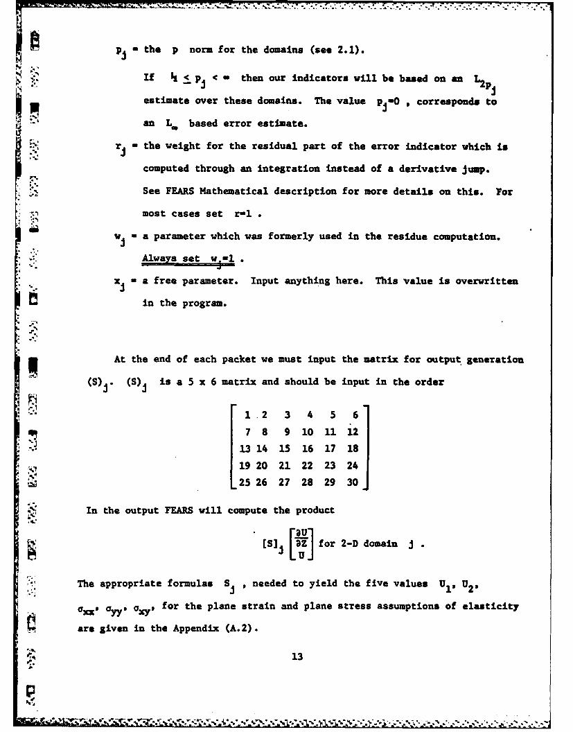
At the end of each packet we must input the matrix for output generation
(S)j. (S)j is a 5 x 6 matrix and should be input in the order
1.2 3 4 5 6
7 8 9 10 11 12
13 14 15 16 17 18
* 19 20 21 22 23 24
25 26 27 28 29 30
In the output FEARS will compute the product
[S] [ for 2-D domain j
The appropriate formulas Si , needed to yield the five values U1, U2 .
- Oxx, YY, Oxy, for the plane strain and plane stress assumptions of elasticity
Care given in the Appendix (A.2).• ,13
' ';-,' , - .i'" l - : , 4 r-. -," ' . .- ". - ." ". -,', . --. '.' - '- -'. ."- ; ... .. .-.- '. ."- .'., -•" - - -* • -* -

2.6 Line Integration Boundary Conditions
HNL Is the number of different packages of line integral matrices. These
p line integrals arise from boundary conditions in which traction or pressure
forces are present. These forces can be either globally defined, if the force
4', is in a fixed global direction, or locally defined, if for example, the force
is normal to the boundary as with a hydrostatic force. The vector c should
give the magnitude of the force in the x and y directions, if the force
is global, and in the tangential and normal directions, if the force is locally
defined. The 2 x 2 matrix y is present whenever the force depends on the
displacement (eg. a spring force).
Mathematically the boundary conditions allowed are of the form
[An] + U - ,whr
FaulnI+ = where
3n 0 nX On7 ] LjIi
(nx,ny) is the outward normal to the boundary and L " is defined in Section
4 -a 2.2.
In terms of stresses the boundary conditions are of the form
T + YU - c
where
X]'( M x + M
[Lforce in x direction
[force in direction]
When the forces are specified locally they are transformed into global forces,
which change in direction and possibly magnitude, with respect to the arc
length of the boundary line.
14
; .* ,'er', .- re_; ,. * ** * .2.... . .. . "2"''* ,.. -''""i''''';'", " -, . .; . _ ," ". ." . -," "

After NL is specified, each of the NL packets of line integrals must
be specified. In the line following NL, we must input
I - the index number of the package,
-i = the number of 1-D domains to which this package applies,
I ...,ni - the indices of the 1-D domains to which the package applies.
The next line contains indicators gi, eI where
gi 0, (~ -0 but duy values in the data line for(y
::stbe input,Ll: (Y)i 14 0
e .i - (C)i 0 0 and the values of (e)i describe a local force
on the boundary,
0 , (C)i - 0 but du-my values for the data line (e)i must
be input,
1 , (C)i 0 0 and the values of (c)i describe a global force
on the boundary.
The () I line should contain the entries of the 2 x 2 matrix y in the
order
The (c)i line should contain the four entries cl(p), €2 (p), e1 (q), c 2 (q),
where p and q are the endpoints of the boundary line. If the force is
described globally then Cl is the force in the x direction and E2 is
the force in the y direction. If the force is described locally then c1
and c2 denote the forces in the tangential and normal directions
respectively, to the boundary.
CFor example, suppose we wish to prescribe a force of magnitude M which
makes an angle of a with the tangent. Then the appropriate values for C
15

should be
M cos a, M sin a, M cos a, M sin a.
Furthermore. the angle and magnitude can be changed linearly (with respect to
the arc length) from a and 0 and M0 to M1 , respectively by inputting
S0 Cos a, M0 sin a, MI cos B. M1 sin for .
*2.7 Subroutines for the functions E(xy), D(x,y).
If a8. or j , the indicators for the vectors D and E , are equal
to -1, we must supply a fortran subroutine to define these functions.
The subroutines will read in the values (x(l),x(2)), the global (x,y)
coordinatesof a point and then compute and return the values
S(1) - the exact solution u(l) (if known),
S(2) - the exact solution u(2) (if known),
" D(l)
D(2) the 4 scalar functions comprising the components of the
D(3) vector D ,
D(4)
E(1),1 = the 2 scalar functions comprising the components of the .vector E,
E(2)
W(l) + -+ D (3)
a a 0the derivatives needed for the residue computation.
The subroutine actually has 4 entry points, returning the values S, D, E,
and W, respectively. The calling sequence is
SUBROUTINE ZPMTRU (X, S).1o
DIMENSION X(2), S(2)
(returns the exact solution S(1), and S(2),
16

COMON/FUPAR/NSUP, FUP (12)
(Common block of function parameters. NSUP-the number of parameters,
and FUP(12)-the function parameters--as dimensioned NSUP < 12. These
parameters are input at the onset of the program (see Section 5.2.)
ENTRY DMATX(XD)
DIMENSION D(4)
(returns the components D(l), D(2), D(3), D(4)),
ENTRY EMATX(X,E)
DIMENSION E(2)
: L (returns the values E(1), and E(2))
and
ENTRY DMATXD (X,W)
,, DIMENSION W(2)
"9 (returns the values W(1), and W(2))
This subroutine must be compiled and mapped with the main program. This
is briefly discussed in Chapter 5.
"17
"" 17

Chapter III. Commands and Strategies
3.1 Introduction--Overview of Strategies
Before describing in detail the various options and commands available
U. to the user, we give a brief overview of how FEARS operates. We hope this
will help clarify what each instruction actually does.
Let us assume that the geometry and bilinear matrices have been input.
An initial subdivision is then performed by the program, and a solution is
obtained on this initial mesh. Error indicators are then computed from the
solution values. A status message or REPORT is then printed out for this
initial solution.
After this initial step, the user has many options for subsequent sub-
dividing (refining) and resolving. In FEARS this iterative process of
subdividing and resolving is continued until either the solution obtained
, -? is within a specified tolerance of the true solution, or the user runs out
of computer resou -es (money, time, or storage). Each REPORT message contains
the approximate relative error as part of its output.
Ideally we would like to employ some optimal strategy which will obtain
for us the desired accuracy with the least computer expense. On, one hand,
an "optimal mesh" is always desired, that is, a mesh which will yield the
smallest error in the solution for a fixed number of degrees of freedom. On
the other hand,we would not like to spend too much money in order to maintain
an optimal mesh at each level. For example, it would be very expensive and
.. wasteful if we subdivided only one or two elements at a time and then
recomputed the entire solution after each subdivision. Thus, even though we
. may get a better mesh by subdividing only one element at a time, it would be
a better strategy to refine a larger number of elements, even though the
mesh obtained may be only "nearly optimal". It has been shown *(1) that
*(l)Babuska, I., and Rheinboldt, W. Analysis of finite-element meshes in RMath Comput. 33 (1979), 435-463).
18
' .A * '

(at least for one dimensional problems) a mesh which deviates slightly from
the optimal mesh is nearly optimal in the sense that the solution with this
mesh is nearly as accurate as the solution on the optimal mesh.
Furthermore, one may ask if it is necessary to resolve the problem
globally after each subdivision. For example, there may be circumstances
where only one or two elements will get subdivided, or all the elements to
.-, be subdivided are concentrated in one region. Perhaps it would be acceptable
to resolve the problem locally--either within each element, or only within
a 2-D domain where some subdivision has occurred. The FEARS program allows
us these options.
For example, we can specify that when some element gets subdivided, all
previously obtained solution values will remain fixed, and a new solution
will be obtained only for the node created at the center of the element by
the subdivision. This is referred to as a SHORT path solution. Error
p, indicators are recomputed for only the 4 new elements. SHORT path solutions
are fast and cheap and are recommended when only a few elements are to be
subdivided.
Likewise we may specify some set of 2-D domains, for example, only.Mthose where subdivision has occurred, and then obtain ;. new solution values
only for those 2-D domains. The boundary conditions on the boundary of
the subdomain are taken to be fixed, with displacement values determined
from the previous solution. This type of solution path is in between a
SHORT path and full solution in both expense and accuracy.
Although the user can control the refinement procedure by specifying
which elements are to be subdivided before each solution path FEARS also has
a built in recommended refinement strategy. This strategy is enacted through
the command AUTO (short for automatic). Each time this command is given,
19

all those elements with error indicators larger than some computed threshold
value (see Appendix A3) are subdivided and a new solution is computed. The
type of solution path performed must be supplied bk the user. For example,
(AUTO/i) will refine and recompute the solution globally, and (AUTO/4) will
refine and then perform a SHORT path solution on each refined element only.
For many problems, particularly those in which there are no singularities,
a sequence of (AUTO/i) commands: is the best strategy for obtaining an accurate
solution cheaply. However, when solving problems with singularities, it is
often the case that an AUTO command will refine only one or two elements.
If the mesh already has a large number of elements, producing a new global
solution in this case is not only 6ostly, but also unecessary. In this
case we would prefer performing a SHORT path solution with an (AUTO/4)
instead of a new global solution with (AUTO/i). If the program is being
run interactively, then the user can decide which type of solution should
be performed, since after each REPORT the approximate number of elements
to be subdivided by the next AUTO command is printed.
Unfortunately, if the program is being run as a batch job there is no
a-priori way to determine when an (AUTO/l) or (AUTO/4) should be performed.
FEARS also has the ability to make this choice automatically with the ITER
(ITERATE) command. The ITER command performs n solution paths composed
of (AUTO/I) or (AUTO/4) commands, the choice depending on whether the number
of elements in the new mesh is a certain percentage over the number in the
old mesh (after the last (AUTO/)). This cut-off percentage must be supplied
by the user, but a 30% increase is recommended.
The user also has control over what information is printed out, after
a solution path is performed. For example, with the PRINT command, informa-
tion about the solution at the nodes and a list of elements with their a-
posteriori error indicators may be printed. The OUTPUT command will give a
20

4
list of stresses and solution values at the center of each element.
Two other useful commands are the DUMP command and the CHANGE command.
The DUMP command will cause all information about the problem, eg. geometry,
bilinear matrices, solution values, and data structures for the mesh, to
be saved on a 'permanent file. The user may then restart the program where
he/she left off at any future time.
The CHANGE command causes small changes in the initial problem. This
is useful if one is interested in the effect of perturbing either the
geometry or material properties of the prolem. In this case, the refined
mesh for the original problem will be almost topologically equivalent to
the refined mesh for the next problem. Therefore, instead of using a lot
of computer time by iteratively subdividing and resolving for the new problem,
the refinc4 mesh for the original problem could be used and a final solution
obtained immediately.
Now that the general format has been presented, we describe the user
commands in detail. The computer will always acknowledge that it is ready
to receive a user command by printing the line
•*** COMMAND:
3.2 PRINT Command
The PRINT command is designed to print out information about the• " 0
points- 1, j=,...,NO, the
lines - i4 , J-1,...,Nl, and the
2-D domains - , j-l,...,N2
The format for the PRINT command is
a,b,c
21

61 The value, a, determines the dimension of the domains to be printed.
0-> print about DOs
1 aprint about D s
a. 2-> print about D21 a0 1,
- -> print about D s D 's and D2 ' sI -,
The value, b, determines which index k of D (aj-l) is to be printed.
"b >1 - k , print about Da only.
print all D's .
The value, c, determines how much information is to be printed.
0 print only headings
1 only print data about the nodal points of the 2-D domain(s).C m
2 only print data about the elements of the 2-D domain(s).
3 print all information
For example, the command
-i,-1,3
will cause all information about each 0-D, 1-D and 2-D domain to be
printed. The format of the printed data and its interpretation are
discussed in detail in Chapter 4.
After the execution of a PRINT command the computer will return to
the command mode and print *** COMMAND
22
. *-.. - . . . . . .

., . . .° °. . _: ~ ~~~. .'. . -. ..*. .. * * . . . ° " . ° 7.° 7 -. o ' .. *. -. ° '.o-7 * % " .- o.o" %
3.3 REPORT Command
q The REPORT command accomplishes two things. First of all, it computes
statistical information about the error indicators and sorts the elements
in the order of decreasing indicators. Thus, a REPORT should be performed
. before each PRINT command to ensure that the elements are listed in order.
. Secondly, it prints out a status report on the full domain giving informa-
tion on the number of elements, total energy, error estimator, percentage
of error, number of elements recommended for subdivision, etc. This message
• "is described in detail in Chapter 4-Output.
L4 °3.4 SUBDIVIDE Command
" .. The SUBDIVIDE command is used to subdivide elements. It has the
following format:
cnomputer * COMMAND:
user SUBDIVIDE
computer SUBDIVISION, 2-D PROCESS INDEX:
m.. user J
computer 0=ALL, GT.O.-CUT OFF VALUE,
LT.O. - GIVE ELEMENT LIST
user x
computer ELT LVL R LOCAL COORD ERR. IND PREV ERRIND"
ELEMENT TO BE SUBDIVIDED: IF X < 0
* user el
computer ELEMENT TO BE SUBDIVIDED:
23
% e . # , , ° • . . ° ° . . , •O - . , o . . o .° • o ° - ° . . - , ° , - - . , ,o . ° o ° o o u . . . . .

computer ELEMENT TO BE SUBDIVIDED: IF X - 0
user 0 (zero)
* cccputer. SUBDIVISION 2-D PROCESS INDEX:
* us22
* co"puter 0 - ALL, GT.O. -CUT OFF VALUE,
- LT.O. - GIVE ELEMENT LIST.
LAuser x2
.2
conputer SUBDIVISION, 2-D PROCESS INDEX:
user 0 (.zero)
computer * COtIAND:
The values J1, J2 .""" give the indices of the 2-D domains in which
the subdivision will occur.
The values X1 , X2 ... , determine which elements get subdivided.
*,Xk > 0 -> subdivide all elements in 2-D domain Tk with
L.0 > give an element list and ask for an index of an
element to be subdivided. The program will
continue to ask for an element until the user
* ~returns 0 (zero).
The user may get out of the SUBDIVIDE loop with a 0 (zero).
3.5 DOMAIN Command
*£ The DOMAIN command is used to set up the subdomain on which a solution
path is to be performed. The subdomain defined may be any subset of the
D2 t
24

'0~.... .. ... " "" " - " - " '- " - . " -" --. " .- '. - " ' -'- -. ;
The format is either
(i) DOMAIN
0or
(ii) DOMAIN
N
kls.*.,kN
In case (i) the subdomain defined is the ful domain, and in case (ii) the
subdomain consists of the N 2-D domains k,, k2 ,...,kN • After the command
DOMAIN is returned to the computer, the message
SUBSET OF 2-D'S: NUMBER OF 2-D'S (0 - ALL)
will be printed by the program.
3.6 LONG Command
p The LONG command will obtain new solution values for each node in the
subdomain specified in the DOMAIN command. If the subdomain defined with
DOMAIN is a proper subdomain of the full domain then any points (D1 ,)
which are external to this subdomain, but are internal in the full domain
are considered as fixed with the values prescribed by a previous solution
path. Also, error indicators of elements which are not in the subdomain
are not recalculated.
The format for this command is simply
LONG.
3.7 SHORT Command
The SHORT command performs a subdivision and a short path solution
on each element specified. When an element ej is specified it is sub-
divided into 4 sub-elements, and solution values are obtained for only
the new node formed in the middle of e * This solution is computed by
25
--P*~* ~ *,*~'

. ....* .. . *.. . '... %- .. , S/ / .-. .,. . .
*solving the problem on the 4 sub-elements with linear boundary conditions
on the boundary of e determined by the 4 cornerpoint solution values
previously determined on e
2 14 24
... 7 8
F iE r 1 3Figure 3.1. Short path subdivision of element a .
In the figure we solve for the circled node in the center having the
previously obtained solution values at 1, 2, 3, and 4 and the values at
5, 6, 7, and 8 are obtained through interpolation. The new error indicators
for he four new elements created are computed in the following way.
Let F denote the father element (to be subdivided) and S1 , S2, S3 ,
and S4 the four sons generated from subdividing F. Let E(F) denote the
error indicator for the father element, and P(F) the predicted error
indicator for the four sons of the father (see Figure 3.2). Appendix A.3
describes how this predicted error indicator is computed.
S2 S4
S S3
Figure 3.2. A father element subdivided into four sons.
We then compute the error for each son E(Si) by the formula
E(Si) = min(aE(F) P(F)), where
a " .55 by default, but can be changed by the user with the SHEF command
26
......... ............................. ...

(see Section 3.16), or at the start of the program (see Chapter 5).
The format for the SHORT command is similar to the SUBDIVIDE command.
cempute2' COMMAND
user SHORT
u puter 2-D DOMAIN PROCESS INDEX:
,er
cc puter ELT LVL R LOCAL COORD ERR. IND PREV. ERR. IND.
e-' el rY I P
*o Onputer ELEMENT TO BE SUBDIVIDED AND SOLVED
user e
orputer ELEMENT TO BE SUBDIVIDED AND SOLVED
user @EOF
-canputer 2-D DOMAIN PROCESS INDEX:
user2
user @EOF
ccenputer. 2-D DOMAIN PROCESS INDEX:
user @EOF
caiirputer *** COMMAND
3.8 AUTO Command
The AUTO command, short for automatic, is a powerful and useful user
-" command. It performs the subdivision, sets up the subdomain, performs a
solution path, and prints a new report.
27
..-.. "

The format for the AUTO command is
AUTO
x (if J < O)
If J > 0 each element having an error indicator which is greater
then or equal to a computed threshold value is subdivided.-SIf J < 0 another value X must be input and all elements having an
error indicator greater than or equal to X will be subdivided.
The value of J determines which type of solution path to take.
J - ± 1 "> Obtain a new solution for the full domain.
J - ± 2-> Obtain a new solution for the subdomain composed of those
2-D domains where subdivision occurred.
J - ± 3-> Obtain a new solution for each 2-D domain individually
where subdivision occurred.
J - ±4 =-> Perform a short path solution for each element subdivided.
Thus, if we wish to subdivide all elements of our full domain and
-'4 resolve the problem globally we could use the command
AUTO
"'" -1
a 0.
The same effect could be accomplished with the sequence of commands:
SUBDIVIDE
1
0.
2
0.
N2
28

0.
@EOF
DOMAIN
1' 0
,, *, LONG
.I REPORT
When using the AUTO command, it is important to understand how the
threshold value is computed. Appendix A.3 contains a detailed explanation.
Actually we compute a threshold for each 2-D domain and then use a global
threshold being the maximum of all the 2-D domain thresholds. All elements
= above the global threshold are then subdivided in the AUTO command (if
J> 0).
-- 3.9 ERROR Command
The ERROR command recalculates all error indicators using the solutions
last obtained and generates a new report. It should be used after repeated
short path solutions in order to obtain more accurate error indicators.
q3. 10 DEBUG Command
The DEBUG command was initially used as a debugging aid, and this
option is still available. However, the user may find it more important
in its ability to print a list of subdivided elements and/or its control
of the output.
* The format for the DEBUG command is
ecputer * COMAND:
user DEBUG
user IPR(l) , IPR(2),...,IPR(8)
Where IPR(l),...,IPR(8) deal with the following:
29

IPRMl) - subdivision element list, short path debug.
IPR(2) - debug error calculation,
U IPR(3) - debug matrix assembly,*R, -"
" : IPR(4) - debug matrix decomposition,.
IPR(5) - debug matrix solution,
IPR(6) - debug back substitution,
IPR(7) - echo input,
IPR(8) - automatic elemental output control.
The values IPR()...IPR(8) should be specified as follows:
IPR(l) - 0 do nothing,
* ,. 1 print a list of the elements which were subdivided
before each solution path,
2 print out short path solution debugging information
-k record the subdivision element list on file with FORTRAN
-I ;unit number k . File k must have been properly
' ,assigned to the run.
-,IPR(J) - 0 donot print,
{ print only summary, (For -2;...,6.)
f print all information,
IPR(7) 0 o not echo input,
- "11 echo input,
IPR(8) - 0 no print,.no file write,
1 print, no file write,
2 no print, file write,
' "3 print, file write.
The parameter IPR(8) causes the listing of the OUTPUT information
(see Section 4.6) to be, either printed, or written on FORTRAN unit number
.' t17, after each AUTO command.
30
Ui = ," It T'% % -% ' ' -. " --" ' '' '. . '""". ". ". --. "". . . ,_- ". '. '

The program also asks for the values IPR(l),...,IPR(8) at the beginning
of each run, and the DEBUG command offers a way to change the initial values
5 of these parameters.
3.11 OUTPUT Command.
The OUTPUT command will have the effect of temporarily changing the
parameter IPR(8) and immediately performing the file write and/or print as*
w '
desired. The format is
cemputer **** COMMAND:
4. user OUTPUT
user n (n-l, 2 or 3)
This effect is only temporary. If a new AUTO command is performed the
print and/or file write will be done as specified by either the last DEBUG
command, or by the initital value given IPR(8) at the start of the program.
3.12 DUMP Command
The DUMP command allows us to save the present data structures, mesh,
solution values, etc. in some file so that the problem can be restarted
from where we left off at some later time. The format is
DUMP
F
where F is an integer indicating some fortran unit number. Since unitsr.4.- 10-17 are already used in the program, units 18 and up may be used here.
These files should all be initially assigned before the program run, and
this is described in Chapter 5.
3.13 RESET Command
The RESET command will restart the problem from the time just before
the last DUMP was executed. The format is
.4.4
31
." * . . ."",_."" .".".." ."."..... . .... . . ... .... .'... , '.'-. . ..- " .- -

m | - .t.-. t - -, - . E - .. -. - : . , . . '
"IS RESET
A F
3 where F is the same unit number used with the DUMP command. If you were
presently running another problem the RESET command will destroy your present
run unless you DUMP it onto some other unit number.
3.14 ITERATE Command
The ITERATE command causes the program to take iteration steps,
*composed of AUTO/J command, automatically, with built in termination. These
steps will be either LONG solutions (J-1) or SHORT solutions (J=4).
The format for the ITERATE command is:
computer A COMMAND:
user ITERATE
user n, a
where n(>O) is integer valued, 0, t, a (>0) are real valued inputs. The
I "value n determines the maximum number of AUTO/J commands to be performed
in the sequence.
The value of 8 is used in the decision strategy to determine the
value of J(-l or 4). The decision value works in the following way. Let
EL be the number of elements after the last LONG solution (AUTO/i). Let ES
" be the estimated number of elements in the mesh when the next refinement
occurs. Then if ES < (140) EL, the AUTO/4 command (SHORT) is performed,
without changing the value of EL. Otherwise, if the estimated increase in
elements is 0% or more, an AUTO/I (LONG) is performed which also changes
EL to the new number of elements. Exception to this rule is at the last
step of the iteration steps, when the program always generates an AUTO/1
(LONG solution).
The value t is the maximum allowed time in seconds. The program
* '32
- . . . - . . - . . , . - . - • .-- *.. • ... - - .. -. . .- -. - * . .. . .. . . -

assumes that the time needed for an AUTO/1 (LONG) step is linearly dependent
*:.. on the number of elements E ;
T i C * E
where the factor C is derived from a previous AUTO/i step. If Ti and the
previously accumulated time of the iteration process is equal or greater than
the given t value, then a last step, AUTO/i, is performed to assure a LONG
solution before returning to the user's next command.
The value a is the required relative accuracy. Again, if a has
do been achieved in the sequence of AUTO/J steps, the program assures that the
last step has been a LONG solution before returning to the user's next
command.
During the sequence of AUTO/J steps, it may happen that the available
data storage area is exhausted due to the increasing number of elements. The
required storage areas are also estimated by assuming linear dependency on
the number elements, although this may not be very accurate.
Thus, an ITERATE command causes a sequence of AUTO/J steps, where the
number of steps is determined by one of the four factors:
Mi) n - given maximum number of steps (no message is printed)
(ii) time allowance (t) is exhausted
(iii) accuracy (a) achieved
(iv) storage is exhausted
If one of the last 3 cases occurs, the appropriate message is printed.
3.15 CHANGE Command
The CHANGE command allows the user to make modifications in either the
bilinear form, geometry, or function parameters, while keeping the mesh generated
from solving the original problem. This command is useful, if for example, the
problem of optimal design is of interest.
-33

A problem is solved with some initial geometry using the FEARS program
and an optimal mesh is created for this problem. It may be of interest, for
example, to determine how the maximum stress is altered by making a perturbance
of the geometry. With the CHANGE command, this perturbed problem can be solved
with just one solution pass, using the final mesh of the original problem.
Suppose that the final mesh of the original problem was saved on file
k by using the DUMP command. After calling the FEARS program (see Chapter 5)
you will first be asked to supply the 8 DEBUG parameters IPR(l)-IPR(8).
After supplying these values the computer will respond:
corputer PROGRAM INPUT DATA IS ON
FILE NUMBER =
to which you should input
user k
k is the file number on which the old mesh was stored.
You will then be in the command mode as the computer will
respond
**** COMMAND:
To use the CHANGE command the user's response is
user CHANGE
The program will then shift back into the input mode and
ask for the function parameters, ID Number of the problem,
P-NORM for the full domain, and then the geometry and
bilinear forms. Here the data should be prepared with
the appropriate changes and input. The program will then
immediately obtain a solution for the new problem using the
previously saved mesh. A REPORT will be given and the
program will return to the command mode.
34
' :. .- ,,-..; -.... ,-.-.- . ... , ,-,....-.... ... .-. - . ....- - . -.. .. ..... . .-. ,,..,.

t~.7
3.16 SHEF Comand
"*" SHEF stands for short 2 ath error factor. This command allows the user
to prescribe the value of a which is used in the short path error calcula-
tions (see Section 3.7). The format for the SHEF command is
caputer *** COMMAND
user SHEF
user a
where a > 0 is real. If this command is not used the default value for
a is 0.55.
3.17 STOP Command
The STOP command causes the termination of the program execution, thus
it should be the last given command:
computer **** COMMAND
user STOP
3.18 ERIT Command
The ERIT command changes the way one of the error terms is calculated
for elements adjacent to internal 1-D domains. This error term is based
on the differevce of derivatives of the solution across the interfacing
1-D domain. Initially in the normal (ON) position, the difference of
derivatives is computed form the two adjacent 2-D domains; while in the OFF
position, the difference of derivatives are estimated internally in the
* -appropriate 2-D domain. The format of the ERIT Command is
computer **** COMMAND
user ERIT
iwhich causes the change of position, from ON to OFF, or OFF to ON. This
command is particularly useful when the problem contains an interface
separating two 2-D domains with vastly different material properties.
35
...........................................

3.19 MESH Command
The MESH command is similar in purpose to the CHANGE comand, i.e., to
get solutions for a slightly changed (in geometry or material constants)
problem. The use of the MESH command requires that the subdivision element
list of the original problem has been saved by the DEBUG command
DEBUG
Vduring the iteration process on file k , where k is a Fortran unit
number properly assigned to the run. If this has been done, one can use the
MESH command after the initial input (geometry, bilinear forms) to recreate
the saved mesh structure for the modified problem by
cc- o puter * COMMAND
user MESH
user k
Note, that the MESH command only recreates the mesh according to the data
stored on file k and does not obtain a solution on it. Then it should
be followed by a LONG command if the user wishes to obtain solution on the
recreated mesh.
3.20 INIT Command
The INIT command reinitializes the program and expects initial input
as a new start without asking for the output option.
36
-- -. . . .... ... -, .. .. _. " -. :- ,'_ ' :. . _ .. . . .". . .- •" . . " - ..

CHAPTER IV. THE OUTPUT
4.1 Introduction-CGlbal and Local Coordinates
Recall that FEARS takes a unit square and maps it onto each 2-D domain.
All computations and mesh refinements are actually computed on this unit
square under the appropriate transformation. The coordinates (U,n) on the
unit square are called the local coordinates and the corresponding values
(x,y)-(x(&,n), y(g,n) are the global'coordinates.
x (xy) )
y
(0n0) X
: Figure 4.1. Local and Global coordinates for a 2-D domain.
. Inside this unit square all refinements, element ordering, etc., takes place.
4.2 Numbering the Mesh of a 2-D Domain
In order to help read the printout, a description of how the elements and
nodes are indexed is given. This will be a great aid in reconstructing the
mesh and hence in locating elements and their neighbors.
The initial subdivision is numbered in the following way:
3 5
2 4
Figure 4.2. Numbering for initial subdivision.
37

The nodes and elements are numbered together--the index 1 corresponding to
the node in the center and the indices 2, 3, 4, and 5 number the 4 elements.
0 USuppose that element 2 gets subdivided. Then index 2 will correspond
to the node formed at the center and the next available indices 6, 7, 8, and
9 will be used to number the 4 now elements created (see Figure 4.3a). Note
that the two circled points are not numbered. These points are irregular
points without degrees of freedowwhose solution values are obtained through
interpolation. Generally, regular points (nodes) are those which lie at the
corner of 4 elements and are always numbered. Irregular points lie at the
corner of only 2 elements and on the side of some other element and are not
numbered.
Suppose next we subdivide element 3. Then index 3 is a point and the
next 4 indices 10, l, 12, 13 number the 4 new elements created (see Figure
4.3b). However, note that the point with local coordinates (.25, .5) is now
a regular point and hence gets the next available index 14.
Finally we present the numbering after elements 4 and 5 get subdivided
in Figure 4.3c.
11 13 11 13 21 23
3 55- -10 12 10 12 20 22
.' ""
7' 9 7 9 16 18
4 4 - -
6 8 6 8 6 8 15 17
a b c
Figure 4.3. Numbering of refined meshes.
38. . .

A listing of the elements subdivided at each level will be output if
the parameter IPR(l) is set to 1 with the DEBUG command (see Section 3.10).
4.3 The PRINT output
The PRINT command will cause data to be printed about the points (D 0 's),
1, 2,lines (D s), and 2-D domains (D1 s)•
4.3.1. Printing the Points (0-D domains)
The format for the data about the 0-D domains of the geometry is as
follows:
<<< O-D COORDINATES SOLUTION ERROR BDRY EXT
1 Xl Yl U1 v1 eu1 ev1 b1 exl
2 x2 y2 u2 v2 eu2 ev2 b2 ex2
0 xNOYNO uNoVNO euNOeNO bNO "x0
The information under the heading
O-D - gives the index number of the point,
COORDINATES - gives the global (xy) coordinates of the point as specified
by the geometry input,
" SOLUTION - gives the computed solution values of the point,
ERROR - gives the error between the computed and exact solution if
the exact solution is known and supplied in the subroutine
ZMPTRU,
BDRY - gives the boundary conditions of the point as specified by
the geometry input, and
EXT - indicates if the point is internal (0) or external (1) to
the full domain.
39
S-2

4.3.2 Printing the lines (1-D domains)
The format of the information about the line with index J is
<<< 1-D INDEX: J B: b, E: ex, l/R: pip
FROM aj TO b PTS: p, R-PTS: rp
p POINTS:
PT R LOCAL GLOBAL COOR SOLUTION ERROR
1 r Pl Xl1 Yl U 1 v 1 eu1 evl
.-.. rp Pp Xp yp up vp ep vP r p
On the top line the value after
B: gives the boundary condition of the line as specified by
the geometry input,
. E: indicates if the line is internal (0) or external (1)
l/R:' gives the signed reciprocal of the radius as specified by the
. . geometry input,
- FROM TO: gives the two indices of the O-D domains forming the endpoints
of the line,
" PTS: gives the number of points on the interior of the line
arising from the mesh, and
R-PTS: gives the number of regular points.
Next, a list of data about the points lying in the interior of the line
arising from the mesh is printed. The data under
PT - gives an index of the point in the order it was formed,
R - indicates if the point is regular (3) or not (0, 1 or 2),
" LOCAL - gives the local coordinate of the point on the line--the
O-D aj has a local coordinate 0 and b. has a local coordinate 1.
40
...................

GLOBAL COORDINATE - gives the global (xy) coordinate of the point,
SOLUTION - gives the computed solution values at the point, and
ERROR - gives the error between the computed and exact solutions if
the exact solution is known.
4.3.3 The 2-D Domain Printout
The format for the printout of 2-D domain J is
<<<2-D INDEX:J CORNERS:C 1 C2 C3 C. NUMBER OF POINTS:NP ELEMENTS:NE ENERGY:
ELT.SIZES:S 1S2S3S4S5 S 6S 7 8 SMALLER SIZES:S 9 ,MAX.ADJ.RATIO:
ERROR INDICATORS,TOTAL: M , M, THRESHOLD:'
HEAD- DISTR. BELOW MEAN(_) :" INGDISTR. ABOVE MEAN C_):
DISTR. ABOVE PRED (_):
TIME, ASM& DEC: , BCK: , THR: , TOTAL:
*:U. STORAGE, MEMORY: , AUXILIARY!
PNT LOCAL COORD GLOBAL COORD SOLUTION ERROR
Pl 1l X y U 1 V1 eul evl
-... .. . .
N P NP NP xNP NP uNP VNP euNP evNP
ELT H R LOCAL COORD ERROR IND. PREV. ERROR. IND.
EH 1 R, C1 11 ERR, PER! 1
ENE NE * R EE ERRNE PERE
' In the top line the value(s) after
CORNERS: gives the 4 cornerpoint indices as specified by the
geometry input,
S.41

NUMBER OF POINTS: gives the number of regular points (NP) of the mesh in the
' :°.': 2-D domain J.,
ELEMENTS: gives the number of elements (NE) in the mesh, and
ENERGY: gives the energy of 2-D domain J.
In the next line
ELT. SIZES: gives the number of elements in the domain having a side-2-2.... -8
of length 2 1 2.. respectively,
SMALLER SIZES: gives the number of elements smaller than 2-8 , and
MAX.ADJ.RATIO: gives (in power of 2) the maximum of ratios of sizes
of two adjacent elements in the 2-D domain.
The next line gives the sum, maximum, mean, and threshold value for the
error indicators of the elements in the 2-D domain.
The following three lines give statistical information on the error
indicators. The value in parenthesis gives the total, and the following 8
numbers give the number of elements in 8 standard deviations from the mean
or maximum predicted value.
The line which gives the TIME breakdown is discussed in Section 4.4.
After the storage requirements are printed, a list of the nodal points
of the mesh in the 2-D domain are given. Included are the index of the point
as determined from the numbering order described earlier, as well as the
point's local coordinates, global coordinates, computed solution values,
and the error of the computed solution (if the exact solution is known and
defined in ZMPTRU). Only regular points are listed.
After the nodal points are listed, the elements are listed in order
1of decreasing error indicators. The indices of the elements are determined
through the same numbering system as the nodal points and this numbering
order was described earlier. Also included are
• ,42

-. . - . . . . . . . . . . . . .
H - indicating the size of the element (2
R - indicates the regularity of the cornerpoints of the element, e.g.
R-3 corresponds to all regular cornerpoints (see Section 4.2).
LOCAL COORD - the local coordinates of the center of the element,
• '. ERROR IND. - the error indicator for the element, and
PREV.ERR.IND. - the previous error indicator. See Appendix A.3 for
further details on the previous error indicator.
m 4.4 The TINE: breakdown
-" ": FEARS uses substructured solving, obtaining solutions first for those
nodes on the 1-D and O-D domains and then backsolving to obtain solutions
for the nodes in the interior of each 2-D domain. In order to better
. :understand the TINE breakdown, write the assembled global stiffness matrix
in the form:
A, B I X12 12
A 3 B X -Y
2 B2 X2 2"
A 3 x 3 3
AAN 2 BN2 XN2- YN2
B T BT B T C YB1 2 N2 XDB
where X correspond to the unknowns in the interior of 2-D domain i, and IL
"" BD
the unknowns for the O-D and 1-D domains.
With the 2-D domain print command, the line starting with TINE lists
* ASM & DEC: the time for the assembly and LU decomposition of Ai°i
BCK: the time for the backsubstitution for the unknowns in 2-D domain i.
THR: the time for computing the error indicators, and
* TOTAL: the sum of the above three times.
S43

The REPORT print lists
EXECUTION TIME:
SUBDIVISION: the time of subdivision for the full domain,
2-D MATRIX SOLUTION: the sun of the ASM & DEC times described above for
each 2-D domain,
BDRY MATRIX SOLUTION: the time for solving C* • BD Y YBD where C, YBD
are C Y YBD modified by the 2-D partial decompositions.
- 2-D ERROR CALCULATION: The sum of the THR times.
At the end of an AUTO command the ***AUTO TIME gives the sum of the 4
execution times plus overhead.
4.5 The REPORT printout
The REPORT has the format
•**** FULL DOMAIN *****
NUMBER OF POINTS: NP NUMBER OF ELEMENTS. NE
,1 ENERGY NORM: NM ENERGY: ENG
ERROR ESTIMATOR: EST RELATIVE ERROR: REL
MAX.ERROR INDICATOR: MAX BY 2-D INDEX THRESHOLD: TH
APPROXIMATE NUMBER OF ELEMENTS TO BE SUBDIVIDED:
- 2-D NO. OF ELEMENTS
2 S2
N2 SN2
STOTAL T
STORAGE SIZES; MAX, CORE-_ , TOTAL- , NO RECORDS-_
BDRY MATRIX -
* EXECUTION TIME:, SUBDIVISION: , 2-D MATRIX SOLUTION:
44'.: " ,;: : . - -, .' - .,. . . . ... ... .. . .. .. ... . . . .- - . . ._ _ . ._ . ... . -. -. .. -

Si- BRDY MATRIX SOLUTION: , 2-D ERROR CALCULATION:
Here
NUMBER OF POINTS: gives the number .of nodes in the 0, 1 and 2-D domains
have at least one degree of freedom,
NUMBER OF ELEMENTS: gives the total number of elements in the full domain,
ENERGY NORM: NM - where
ENERGY: ENG
ERROR ESTIMATOR: gives the error estimate for the full domain,
RELATIVE ERROR: REL - NM/EST.
The next line gives the maximum error indicator, the 2-D domain it is in,
and the threshold value for automatic refinement.
Next is a list of the number of elements in each 2-D domain which will
be subdivided if the threshold value is used for subdivision.
Storage size information is then given and finally a breakdown of the
times as discussed in the previous section.
4.6 The OUTPUT printout
In this section we describe the data either printed or file written,
with either the OUTPUT command or by previously setting IPR(8) in the DEBUG
command or at the program start. The data printed will be a list with the
headings.
2-D ELT H LOCAL COORD GLOBAL COORD ERR.IND OUTP(l) . . . OUTP(5)
The column headed with
-; 2-D gives the index of the 2-D domain that the element is in,
ELT - gives the index of the element,
* H - indicates the element size (-2
LOCAL COORD GLOBAL COORD - gives the local and global coordinates at the
center of the element,
45
. -o .
'.•.% \ -. . . . - -".

ERRIND - gives the error indicator of the element,
OUTP ():
pOUTP(2)OUTP(3) will give the stresses ax, ayy, xy, and solutions u 1 , u2 at
OUTP(4) center of the element if S was given for the elasticity problem.
OUTP(5)
These last 5 values are determined by the output matrix S given in the bilinear
matrix input. The 5 values printed are determined by
* Faul rOUT(1)mI [ ...
5x6L~ om()OUT1P (5)]6xl 5xl
The appropriate S for elasticity problems is given in the Appendix.
* 4.7 DUMP-File output
p A sequential binary DUMP-file is generated by the DUMP command. This
file can be used as input for FEARS (see Sections 3.13 and 3.20), or as input
*" .i for various postprocessors. The order of the binary records on the file are
as follows:OP
1. Summary record of the problem (16 words)
2. Last long path history record (40 words)
3. Function parameter record (N+1 words where N is the number of
parameters)
4. 0-D summary/records (8 words/records, N0 records)
5. 1-D summary records (18 words/records, N1 records)
6. 2-D Summary records (25 words/records, N2 records)
7. For each 1-D domain with non-fixed boundary condition:
* 7.1 1-D data record (8k words, where k is the number of points
." on the l-D)
46L2

7.2 If y,c matrices were defined for the 1-D then y,c data
record (13 words)
.. 8. For each 2-D domain
8.1 2-D data record (4k words, where k -is the number of points
and elements in the 2-D)
* 8.2 Bilinear form data record (125 words)
Details on the fields of records can be found in the Program Documentation.
b-7
m
L,
71.7
d...

CHAPTER V. STARTING THE FEARS PROGRAM
This chapter describes the UNIVAC 1100 EXEC control cards necessary
to run the FEARS program. There are two elements and one file which are
of concern:
Absolute element: CKM*FA.A
Relocatable file: CKM*RE.
Map element: CKM*SE.MAP
The names of the above elements (file) may change by the actual installation.
The absolute element contains the absolute program with dummy, zero valued,
function routine for E(X,Y),D(S,Y) which can be run if that routine is
satisfactory by
@XQT,F CKM*FA.A
Otherwise, section 5.2 describes how to set up an absolute program with the
help of the Relocatabli file and Map element to incorporate the user's
supplied function routine.
Section 5.1 explains the necessary file assignments to be included prior
to the run of the program. Section 5.3 describes the necessary initial
inputs for FEARS before the geometry, bilinear matrices and command inputs
are given as described in chapters 1, 2 and 3, respectively.
5.1 File Assignment
FEARS uses six temporary files (11 to 16) with all runs which should be
assigned by
@ASG,T 11.@ASG,T 12.@ASG,T 13.@ASG,T 14.@ASG,T 15.,///512@ASG,T 16.
Four other files may be used depending on the actual run and commands given
48

for the run. These files should be catalogued files with user's given names.
These names should be associated with the fortran unit number by @USE:
@ASG, A file name.@USE n., file name.
where n is the FORTRAN unit number. The four files are as follows:
• (i) Output file - If the OUTPUT command is used, see 3.11, or IPR(8) was
given as 2 or 3 in either the DEBUG command (see 3.10)
or initially (see 5.3), the file should be assigned with
n-17 . At the termination of the run, the file will
contain the stresses as described 4.6.
, * (ii) Mesh file - This file is generated as output file if IPR(l) = -n as
given for the DEBUG command (3.10), it is used as input
file for MESH command (3.19 It is recommended to use
n - 18.
. (iii) Dump file - This file is generated by the DUMP command (3.12). Since
.* present and future postprocessors use this file as input
file, most of the use of FEARS is anticipated to use this
file. Recommended n - 20.
(iv) Reset file - This input file is assumed to be generated by a DUMP
command in previous run of FEARS. The file is used either
initially (5.3) or by the RESET command (3.13). Recommended
n - 21.
5.2 Preparation for Execution
When the user has to incorporate his/her function routine (see 2.7), then
a new absolute program of FEARS must be generated. The recommended steps to
Lbe taken are as follows:
(i) Write the function routine according to the speficication given in 2.7.
Compile the symbolics using the ASCII FTN compiler to generate the
49
..................'-. . -. ... " .

* relocatable element. For further on, it is assumed that F.FXY is
element name of this relocatable element.
* ~*'**(ii) Using the editor,
@ED (CQM*SE.MAP,M
change the Map element into M
-user*
* -computer @MAP,IN *CIC*FA.A
user *(C /CKM*FA/F/
computer @MAP, IN ,F.A
*N 2
computer IN CK1*RE.FJNC
user * / CKM*RE.FUNC/F.FXYI
computer IN F.FXY
Uuser *
*computer editor signs off
user @ADD M
-computer MAP
END MAP. ERROR 0 0 .
The above sequence places the new absolute element F.A in the users
file.
-(iii) After the appropriate assign statements, see 5.1, the run can be
initiated by
@XQT,F F.A
1.- 50

i7-
.. - .1
Note:
U The geometry and matrix inputs can be prepared separately in file
elements, e.g. in INP.Gl and INP.MXl , respectively. In this case,
the user simply applies the UNIVAC commands
. @ADD INP.Gl@ADD INP.MXl
in the above input stream as input for the geometry and bilinear, error
Ii and output matrices. This technique is especially useful when FEARS is
used interactively.
51
.--.- -.. . . . .
*5 -*'. . .< ....................

5.3 Execution of FEARS
* After the program execution has been initiated by @XQT,F, the computer
will respond
***** F E A R S *****2-D FINITE ELEMENT PROGRAMUNIVERSITY OF MARYLAND. 1981.
MAXIMUM ALLOWED SIZESNUMBER OF O-D, 1-D, 2-D: 34 49 16NUMBER OF POINTS ON A 1-D: 31
-* NUMBER OF POINTS AND ELEMENTS IN ONE 2-D: 482MATRIX STACK SIZE FOR ONE 2-D: 8800BOUNDARY MATRIX SIZE: 14000
SHORT PATH ERROR-FACTOR - .55000PRINT CONTROL INTEGERS (8):IPR(1) - PRINTS DURING SHORT PATH, SUBDIV.
" NEG. K - RECORD SUBD. ELEMENTS ON FILE KIPR(2) - PRINTS DURING ERROR CALCULATIONIPR(3) - PRINTS DURING ASSEMBLYIPR(4) - PRINTS DURING DECOMPOSITION
- IPR(5) - PRINTS DURING MATRIX SOLUTIONIPR(6) - PRINTS DURING BACKSUBSTITUTIONIPR(7) - REPRINTS INPUT
. IPR(8) - AUTOMATIC ELEMENTAL OUTPUT CONTROLIPR(J) ,J-,. . .,8:
The user now should input the 8 integer values IPR(1) - IPR(8) as discussed
in the DEBUG command, e.g.
.. : 0,0,0,0,0,051,0
Next the computer will respond
PROBLEM INPUT DATA IS ON
FILE NUMBER :
The user should input zero:
0
if this is a new problem, or the Reset file number, e.g.
21
Con which all the data at some stage of a problem was saved by the DUMP command.
In this case, the computer will respond
52

**** COMMAND
and the program will be in the command mode.
Otherwise (in case of a new problem), the computer will respond
FUNCTION PARAMETERS: N,Pl,...,PN(N>O):
and the user should input an integer N>0 , and N parameters for use in the
user defined functions routine (see section 2.7). If no parameters are
required, the dummy values 1,0,may be input.
The computer will then respond
ID - NUMBER OF THE PROBLEI:
and any integer response from 1 to 999999 will suffice.
The next computer response is
P-NORM FOR THE FULL DOMAIN:
The P requested here is the same one as in (2.1). If an L2p norm is of
interest in measuring the errors then the value P>.5 should be input. An
L norm will be used if 0. is input. Usually P-1 which corresponds to
the standard L2 energy norm.
The computer will then respond
PROBLEM ID:
DATE:
P-NORM:
GEOMETRY:
At this point the geometry should be input in the format described in chapter
1, i.e., starting with number of O-D domains and ending with the last 2-D
domain description line.
If no errors are detected the computer will respond
GEOMETRY ACCEPTED
BILINEAR, ERROR, AND OUTPUT MATRICES:
53
....

At this point, these matrices should be input in the format described in
Chapter 2.
J ,l The computer should then respond
MATRICES ACCEPTED
INITIAL SUBDIVISION, 1 OR 2:
The value 1 will cause each 2-D domain to have 4 elements and the value
2 will cause each 2-D domain to have 16 elements for the initial mesh.
Finally the computer will respond
INITIAL SUBDIVISION ( ) FOR 1-D PERFORMED
INITIAL SUBDIVISION ( ) FOR 2-D PERFORMED.
The program will then obtain an initial full solution path on the entire
domain, print a REPORT and respond
**** COMIND
signifying that it is ready for user commands.
Once in"comand mode, further actions are governed by the user's
commands as described in Chapter 3.
54S. . . o. . . , -

APPENDIX A
A.1 Sainple Geometry
In this appendix sample domains and their FEARS geometry input are
presented.
Example 1: Quarter Ring I subdoinain
LAO 0
+34
Figure A.l. Quarter Ring
7"he geometry Input for Figure A.1 is:
5 410o.9.5,1,0.00.
2,0. ,l. ,1,0. ,0.
3, .5,0. ,2.0. sO.
4*1.*.O. ,290.90.
4
1,1,3,0,2.
2,2,4,0,1.
3,1,2,1,0.
4,3,4,2,0.
1
iii 1,1,2,3,4
* Note that the boundary condition on line index 1 is specified as free. The
* force present (indicated by arrows) is specified in the bilinear matrix
* input.
55

.7 .... . ..
Example 2: Unit Square - 4 - sub domains
II -
3_, -O- _ t_
6 12 7
:: Figure A.2. Unit: Square
99
The geometry input for Figure A.2 is:
1,0.,0.,3,0.,0. 4,5,8,0,0.
2,0.,.5,3,0.,0. 5,1,2,3,0.
3,0.,.,3,0.,0. 6,4,5,0,0.
4,.5,0.,0,0.,0. 7,7,8,3,0.
5,.5,.5,0,0.,0. 8,2,3,3,0.
." 6,.5,1.,0,0.,0. 9,5,6,0,0.
7,1.,0.,3,1.,0. 10,8,9,3,0.
8,1.,.5,3;1.,0. 11,3,6,0,0.
9,1.1.,3,1.,0. 12,6,9,0,0.
12 4
1,1,4,0,0. 1,1,2,4.5
2,4,7,0,0. 2,2,3,5,6
3,2,5,0,0. 3,4,5,7,8
4,5,6,8,9
56
• -; ,. , -. . j ..- - ..- .-; -. -. :, . -. .. , . _. " . . . . . ." ". " " . " -.' ,.' - .-' -'. . . / - .'.". ..- ".. ....".. . .'.". ."." "".. .' ". .". .... ...". ."." ,

Example 3: Disk
-i 0w LL 2 0
* '1
Figure A.3. Disk with hyrsai force.
*8 5,5,1,0,0.1,-.4,0. 9090.,0. 6,6,2,0,0.
2 9 O ..4 , 0,0. 90. 7,3,7,0,0.
39.490.9090.90. 8,4,8,0,0.
4,0.,i-.4,0,O.,90. 9,8,5,0,1.
5.-l. 90. *2,0.,0. 10,5,6,0,1.
6,0.,1.9090.90. 11,6,7p,,1
791.,0.9390.,0. 12,7,8,0,1.
8,009-1.90'0.'o. 512 1,1,2,3,4
1,1,2,0,0. 2,5,1,8,4[22,2,3,0,0. 3,5,6,1,2
3,1,4,0,0. 4,2,6,3,7
4,3,4,0,0. 5,8,4,7,3
57

...* .--- ,-- ... - . .* : -- - , - ' * o -. M
-. -. . . - . * ° . - o
Notice the boundary conditions at points 5 and 7. For this problem,
additional boundary conditions are necessary to ensure uniqueness of a
* solution by eliminating rotations and translations of the solution. Point
7 was picked arbitrarily as the stationary point (u1=u2 --O). To prevent
rotations the vertical displacement, u2 , was set to zero at point 5. It
would be equivalent to fixing the vertical displacement at either point 1
' '-: or point 3 as well.
58
* i*.* ~ . .. - -*.. *.'-* . . .

Example 4; Cracked Square
%Ja
LLILI
U#Z
10 3,36,0,0.
1,o.20.2o,0.10. 4,4,7,0,0.5,5,8,0,0.
2,0.,5,3,.,0.6,6,9,0,0.
3,0.9.5,O00-0. 7.7,10,0,0.
4,0.91.,0,0.90. 812009.5,6,0,0.
5 ' .5 9 . 90 9 .,0 .1 0 , 8 , 9 , 0 , 0 .*6,.5,.5,3,0.90. 11.3,4,0,0.
7,.5,1.,0,0.,0.12670.a 13.9,10,0,0.
bW r81.0.,0,0.,0. 4 or -4
991.9.5,0,0.90. 1,1,2,5,6 1,1,2,8,9
2,3,4,6,7 2,3,4,11,12*3,5,6,8,9 3,5,6,9,10
134,6,7,9,10 4,6,7,12.13
2,2,6,3,0.
59

| 1.'. - - - - - -.
II
Notice that points 2 and 3 have the same coordinates and thus lines
- .2 and 3 lie on top of each other. This represents the two edges of a
crack.
A.2 Bilinear and Error Matrices
A.2.1. The Matrix A Arising From Elasticity
The principle of virtual work for the elasticity equations yields
an integral of the form (6c)TcC , where
_ D
] Fau1
c- au 2 and C-yy aYcau I1 au 2
-"' is the 3 x 3 stress-strain matirx such that
C. a . For the plane strain assumption the
.XY
i matrix C is given by
1- v 01E - 1-v 0
C =(l+v)(l-v)0 0 1-v
2
and for the plane stress assumption
r E- 1 v 0
where E is Young's molulus and v is the Poisson ratio.
60

The corresponding integrand in the FEARS formulation is
ravi Tui-IA---
L3ZJ Aa
Since au au we may
.i U2
axau1" 8U2
ayau2lay
write c Iau where
1 00 01D i 0 0 0 1 (A.1)
•0 1 1 0 .
av0]Also, Sc -D--- Therefore,
- az
( 6 )TC " = ]TD C D[u , from which we have the relationship
ME) , Z- DT CD 37T
AD CD.
P M For the plane strain assumption
1-v 0 0 v
0 1-2v 1-2v
A E 2 2(1+v) (1- 2v) 1-2v 1-2
::.2 2
v" 0 0 1-V ,
and for the plane stress assumption
1 0 0 v
1-2v 1-2v0--0
A- E 2 2A 2_v 01-v L-v
-. 2 2
v 0 0
61
, *, . . "'-' .--. . .."" " ". " " .. • * " " ." . ." " " " "

..... .. .. .. .. .. . . . . . . . . . .. . . . .-. . . ' ' ' I
" " !
A.2.2 The Error Matrix A .
For elasticity problems the matrices (C)j described in Section 2.3
are zero, and so, from (2.1) the error is approximated in the norm
N1U1 2P[ 2{aU] T(A E) [ 3ui J%IllUlll2p- .r'21 ZJ J I ]
To obtain error estimates for the energy norm, simply take (AE) = (A) .J
Suppose, however, that our interest is concentrated on the error in
one of the stresses, say a.x . Since a xx= [1 0 0]oaIa x2. [r T -11 0 0 S 1 0 0
0 0 0]
o ooco
0 [01 T 0
CT[1 o o C
Let Q m~~l 0 0 Thn0 fteerra i u ancnen
_LE TD TC T QCD0 [ U
0 0 0 2 0
0 0 0
where C is the 3 x 3 stress strain matrix, and D is defined by (A.1).
Let Q 1 0 01 Then, if the error a " is our main concern,
-0 00 0 0 .
we should take
For example, using the plane strain assumption with an error in aoxx9
"E " l+v) (1-,) 0 0 0 0
0 0 0 0
V(1-v) 0 0 v2
62
• . . - -. 'o '--. - % ... .. . ,,. -. - -. .,, ,- j, -, - . ,- . "-k. , . . . .- . .-.. . . - -

4- .11 .7-w -i -6- -o -'J
For the error in a yy take Q in (A.2) to be
0 1 0
0 00 and
for a , take Q tobe
C-1
A.2.3 The Output Matrix S
For the OUTPUT printout (see Sections 3.11 and 4.6) the vector printed
is obtained from the multiplication
S 3U where Wi and U are
evaluated at the center of each element. In order for a printout of
a xx a , , u l' u 2 the matrix S should be
Sm E r1 0 0 i 0 0
l V 0 0 1 0 0
L0 1-V 1-v 0J 0 0O 0 0 0 1 0
O 0 0 0 0 1
under the plane stress assumption, and
5- E F1-v 0 0 V 0 0(l+v) (1-2v) V 0 0 1 -V]0O
1-2v 1-2
O 0 0 0
O 0 0 0 0 1
under the plane strain assumption.
63

A..2.4 Sample Inputs
Example 1: A-Matrix: Laplacian
Error norm: Hl seminorm.
Packages: One package for one 2-D domain.au 1 au 2 au2 au1
Output Matrix: u 1 , .53 + a1Sx- g y- 3x Aay u u1 U2
Line Integrations: None.
' 1,1, 1
1, 0, 0, 0, 0
1., o,,o,,1., 0., 0., 0., 0., 0., 0., 0., 0., 1., 0., 0., l.
1., 0., 0., 1., 0., 0., 0., 0., 0., 0., 0., 0.,1., 0., 0., 1.
1., 1., 1,1
1., 0., 0., 0., 0., 0.
0., 0., 0., 1., 0., 0.
0., .5, .5, 0., 0., 0.
"" 0., 0., 0., 0., 1., 0.
0., 0., 0., 0., 0., 1.
p0
.:-S.°
64
. .~,;: - .. ........... -...... •.. -.. . . ..... ... ......-.- -.-... -,..-... -..

Example 2: A Matrix: Plane Strain Elasticity
Error Norm: L2 Energy
Packages: Two packages f or 4 2-D domains.
Package 1: 2-D domains 1 and 2, v, - 0.0, E -1.0
Package 2: 2-D Domains 3 and 4, v - 0.3, E - 1.0.
Output Matrix: aq y a, 9~ u 2 , U2 .
Line Integrations: Local normal force on line 4.
2
1, 29 19 2v 0., 1, 0, 0, 0, 0
1., 0., 0., .5, 0., 0., .5v 0., 0., .5, 0., 0., .5, 0., 0., 1.
1., 0., 0., .5, 0., 0., .5, 0., 0., .5, 0., 0., .5, 0., 0., 1.
1., 0., 0., 0., 0., 0.
1 0., 0., 0., 1., 0., 0.
* 0., .5, .5, 0., 0., 0.
0., 0., 0., 0., 1., 0.
0., 0., 0., 0., 0., 1.
2, 2, 3, 4
10, 0, 0, 0
1.3461538, 0., 0., .38461538,0.,.57692308, .38461538, 0.
0., .38461538, .57692308, 0., .38461538, 0., 0., 1.3461538
1.3461538, 0., 0., .3846i538, 0., .57692308, .38461538,0.
0., .38461538, .57692308, 0., .38461538, 0., 0., 1.3461538
* - 1, 1.,1., 1.
1.3461538, 0., 0., .57692308, 0., 0.
L .57692308, 0., 0., 1.3461538, 0., 0.
0., .38461538, .38461538, 0., 0., 0.
0., 0., 0., 0., 1., 0.65

0., 0., 0., 0., 0., 1.
1PI 1, 1, 4
0, -1
: '. 0., 0., 0., 00
/ 0., 1., 0.# 1.
Example 3: A-Matrix: Plane strain
Error Norm: L for ayy
Packages: One package for one 2-D domain, v 0.0, E - 1.0.
Output Matrix: a xx, y a x7 Ulu 2
Line Integration: None
;. 1
1, 1, 1
1, 0, 0, 0, 0
1., 0., 0., .5, 0., 0., .59 0., 0., .5v 0., 0., .59 0., 0., 1.
0., 0., 0., 0., 0., 0., 0., 0., 0., 0., 0., 0., 0., 0., 0., 1.
0., 1., 1., 1.
1., 0., 0., 0., 0., 0.
0., 0., 0., 1., 0., 0.
0., .5, .5, 0., 0., 0.
"-': 0., 0., 0., 0., 1., 0.
0., 0., 0., 0., 0., 1.
.6 0
66
4i

A.3 Computation of the Threshold Value
When using the AUTO command or the ITERATE command (the ITERATE command
causes a sequence of AUTO commands to be performed), it is important to
understand how the threshold value is computed. Recall that with the AUTO
command, all elements having error indicators above a certain threshold
are subdivided. Because of the remarks made in Section 3.1, we seek a mesh
in which all error indicators are nearly equal.
The most naive way to equalize the indicators would be to simply sub-
divide the element with the largest error indicator before each solution
path. Suppose that the elements in the initial mesh are labeled
1, 2,... ,N
in order of decreasing error indicators. Following our "naive" strategy,
we sould subdivide element 1 into four subelements--l.l, 1.2, 1.3, and
1.4. After resolving and recomputing the error indicator our new list might
be
2, 3,...J 1 , 1.1, J1+l,...,J 2, 1.2, J2+1,...,N
*2' Next, element 2 gets subdivided into 2.1, 2.2, 2.3, 2.4, etc. Suppose element
PO 1.1 has the largest indicator of the first 4J1 subdivided elements. That is,
E(l.l) >E(i.j) for i - 2,...,Jl, and j 19..,4.
Then our strategy would have subdivided the first J elements one at a time,
obtaining a new solution between each subdivision. Clearly, it would be more
efficient to subdivide all J elements at once before obtaining a new
solution. The cufoff at J could easily be determined if we know what the
maximum error indicator would be for the next level of subdivided elements
(in this case E(1.I)). The following procedure is used to approximate this
cutoff value.
67
..-- 47% t *sv •#.Pq •. .. *;-.** . * * .

7- T 7 -7
Suppose that a father element F is to be subdivided into its four
sons--F.l, F.2, g.3, and F.4. (see Figure A.5)
L1.IF3Figure A.5.
The error indicator for the father element, E(F) is then saved as the
previous error indicators for the four sons. It is then assumed that the
errors arising from subdividing the sons .F.1, F.2, F.3, and F.4 vill
decrease by the same ratio as from the previous subdivision. That is, we"" PRESENTuse the recipe: PREDICTION - PREVIOUS x PRESENT. Thus, the predicted error
!indicator for each of the four sons is computed by the formula
P(F.i) - E(F.i) 2/E(F) , for i - 1, 2, 3, 4.
In order to ensure that the predicted error is smaller then the present
3 error we add the condition-
P(F.i) - min((F.i), (.9)2PE(F.i) if p L .5
(.9)E(F.i) if p 0,
where p is the p-norm for the 2-D domain as input in the (Nc) line of
bilinear and error matrix input.
If an element is not a son of some father element, that is, the element
also belongs to the initial mesh, then no previous error indicator is
available. In this case, we make a prediction for the error indicators
upon subdivision of this element F , by the formula
'" (42) 2PE(F) if p > .5
(,/r2)E(F) if p - 0
The threshold T is then calculated by the formula
68

U.4
Tm max PC?)
as T ranges over all elements in the mesh.
.69

• .. APPENDIX B
FEARS Element Postprocessor
The purpose of the Postprocessor is to allow flexible computations of
various functionals on the approximate solution. The functionals can have
-: various structures and can be used for the effective computation of the stress
intensity factors in fracture mechanics etc. At the present the functionals
are on the level of 2-D domains, but will be extended in the future to deal
if with functionals on the 1-D domains also.
A FEARS Postprocessor frame has been set up in the file CKM*ELTOUT.
Both symbolic and relocatable elements for an Element Postprocessor has
t been established in the file. To produce an executable absolute element,
the user must write some subroutines and combine it with the above file.
" .~The FEARS Element Postprocessor reads the RESET filE generated
by the FEARS program using the DUMP command. The Postprocessor requires a
user's written subroutine (with 5 entries). The purpose of the Postprocessor
frame is to relieve the user of the cumbersome task of setting up the data
structure from the RESET file and setting the individual element informationsNneeded for his/her calculations. The frame allows it to process all elements,
or only those which are in certain 2-D domains designated as active 2-D
domains by the user.
-.- Frame alaorithm:
The main program of the Postprocessor frame has the following algorithm:
1. Read the RESET file and set up internal data structure..°
2. Clear activity tags HDlTHP(j) and MD2TMP(k) of all 1-D and
2-D domains, repectively.
3. Call ELTO(MSARY) calls user's initialization routine.
I.: 4. DO I-1 to MSP2 (number of 2-D).
5. IF MD2TMP(I)=O THEN GOTO Next I
P70

6. Set up core sto-age for 2-D index I.
7. CALL ELTI(MD2ARY).
call user's 2-D initialization routine
8. DO J-I,M2SXE (number of elements in the 2-D)
9. CALL ELTX(K,NX,C)
;..* call user's processing routine
10. Next 3
di 11. CALL ELT1E(MD2ARY)
S.. call user's 2-D stary routine
12. Next I
i ~13. CALL ELTO(MSARY)call user's final summary routine
14. STOP
U User's supplied subroutine(s):
The user must s-pply the following five subroutines, or subroutine(s)
with the appropriate entries. Note that the procedures, ZMS, ZMDO, ZMD1
and ZMD2 may be used in these routines. These procedures define data areas,
summary records of the problem. The user may also use procedures ZP2T,
- ZP2OS, ZP21S and ZP2B, which give the data area (restored) for a given 2-D
domain. For proper use of these data, the user should consult FEARS program
documentation.
1. SUBROUTINE ELTO(MSARY)
INCLUDE ZMS
INCLUDE ZM1I
INCLUDE ZMD2
This routine is called as an initialization. The user must set the
active 2-D domains by setting MD2TMP(j) to non-zero with j being the
71

active 2-D domain indices. These indices may be obtained by user's
defined input, or in case of all 2-D's, through a simple loop on J=lMSP2,
where MSP2 is defined in procedure ZMS (summary array of the full domain)
and MD2ARY is defined in procedure ZMD2 (summary records of 2-D domains).
user may also mark the 1-D domains, if needed in later calculations. This
can be done by storing integer values in MDlTP(k) where k is the index
of the 1-D, and MDIARY 1-D summary records are defined in procedure ZMD1. On
-subsequent processing, these integer values may be tested.
The user may define further storage areas needed for subsequent
calculations, also perform any input needed, outputs such as headings, etc.
2. SUBROUTINE ELTl(MA2)
DIMENSION MA2(26)
P This routine is called in the beginning of all active 2-D domains where
the array MA2 is the sumary array of the 2-D domain with MA2(l) containing
the index of the 2-D, MA2(26) the activity non-zero tag set by the user.
3. SUBROUTINE ELTX(K,N,X,C)
DIMENSION X(2) ,C(2,4)
This routine is called for each element in the active 2-D domains where
the user must perform his own calculations. The arguments are input arguments
as follows:
K - index of the element
N - level number of the element in the transfered unit square,
side length h-2**(-N-1)
X(l),X(2) - local (unit-square) coordinate values of the middle
point of the element
72

C(l.j),C(2,J) - solution values at the j'th cornerpoint of the
element where j is defined in order:
2. 1--- 433
Furthermore, the following function/subroutines are also available for use:
H = FUTH(N)'",
side length of the element
: ,CALL ZP2XY(X,Z)
gives the global coordinates Z(1),Z(2)
corresponding to the local coordinates X(l),X(2)
CALL ZP2TRX(X,T,D)
gives transformation matrix T and its determinant D at the
local coordinates X(l),X(2):
n T(l) - d(Z(1))/d(X(1))
T(2) - d(Z(1))/d(X(2))
T(3) - d(Z(2))/d(X(l))
T(4) - d(Z(2))/d(X(2))
4. SUBROUTINE ELTlE(MA2)
DIMENSION MA2(26)
This routine is called after all elements of an active 2-D domains
have been processed by the ELTX routine. This entry allows the user to
print any summary for the 2-D domain, MA2 array is the same as for the
" .subroutine ELTI.
5. SUBROUTINE ELTO(MSARY)
DIMENSION MSARY(16)
73(2

,.. This routin! is called after all elements of all active 2-D's have
n been processed to allow the user to print any summary of his/her
calculations.
.5,7
,.o
a..
474
..............

1ITI