Embed Size (px)
Citation preview

Mary PagnuttiRobert E. Ryan
Innovative Imaging and ResearchBuilding 1103 Suite 140 C
Stennis Space Center, MS 39529
ASPRS 2011 Annual ConferenceMilwaukee, Wisconsin
May 3, 2011
I 2R I nnovative Imaging & Research
I 2R
Spatial resolution determines the smallest set of objects that can be resolved within an image Not simply ground sample distance Depends on Point Spread Function (PSF) or Modulation Transfer
Function (MTF) PSF and MTF are difficult to fully determine in practice Edge targets placed within a scene can be used to
partially evaluate PSF and MTF One dimensional cross-sectional evaluations
2-4-2
02
4
-4-2
0
240
0.2
0.4
0.6
0.8
1
XY
Example 2D PSF

I 2R
Input Image 20 m x 20 m Target
PSF 4 m FWHM
Blurred Image 20 m x 20 m Target
Sampling
GSD 2 m
GSD 1 m
GSD 4 m
+
3

I 2R
Input Image 20 m x 20 m Target
PSF 1 m FWHM
Blurred Image 20 m x 20 m Target
Sampling
GSD 2 m
GSD 4 m
GSD 1 m
GSD 2 m
GSD 4 m
4
+

I 2R
Frequency Domain Modulation Transfer
Function (MTF) MTF at Nyquist typical
parameter
Spatial Domain Relative Edge Response
(RER)
5
1.0
Cut-off frequencySpatial frequency
MTF @ NyquistM
TF
-2.0 -1.0 1.0 2.0
0
1.0Ringing Overshoot
Ringing Undershoot
Region where mean slope is estimated
Pixels0.0

I 2R -2 -1 0 1 20
0.2
0.4
0.6
0.8
1
Distance / GSD
Line
Spr
ead
Func
tion
-5 0 5200
300
400
500
600
700
800
900
Distance / GSD
DN
0 0.2 0.4 0.6 0.8 10
0.2
0.4
0.6
0.8
1
Normalized spatial frequency
Mod
ulat
ion
Tran
sfer
Fun
ctio
n
Nyquist frequency
Edge Response
Line Spread Function
MTF
Differentiate FourierTransform
6
I 2R 7
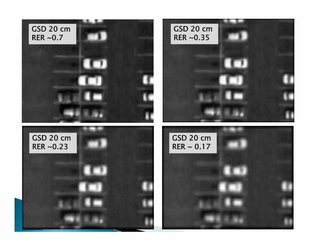
GSD 20 cm RER ~0.7
GSD 20 cm RER ~0.35
GSD 20 cm RER ~0.23
GSD 20 cm RER ~ 0.17

I 2R 8
GSD 20 cm RER ~0.7
GSD 80 cm RER ~1.0
GSD 40 cm RER ~1.0
GSD 60 cm RER ~1.0

I 2R March 8, 20069
3 examples of undersampled
edge responses measured across the tilted edge
Problem: Digital cameras undersample edge target
Solution: Image tilted edge to improve sampling
Superposition of 24 edge responses shifted to compensate for the tilt
– edge tilt angle
– pixel index
x – pixel’s distance from edge (in GSD)Pixels
Distance/GSD
DN
DN
9

I 2R
Most commonly used spatial resolution estimation techniques require engineered targets (deployed or fixed)
Target size scales with GSD Edge targets are typically uniform edges 10-20
pixels long and tilted a few degrees relative to pixel grid (improve sampling) to achieve ~10 pixels across edge Increasing GSD increases difficulty Moderate resolution systems such as Landsat use
pulse targets
10
I 2R
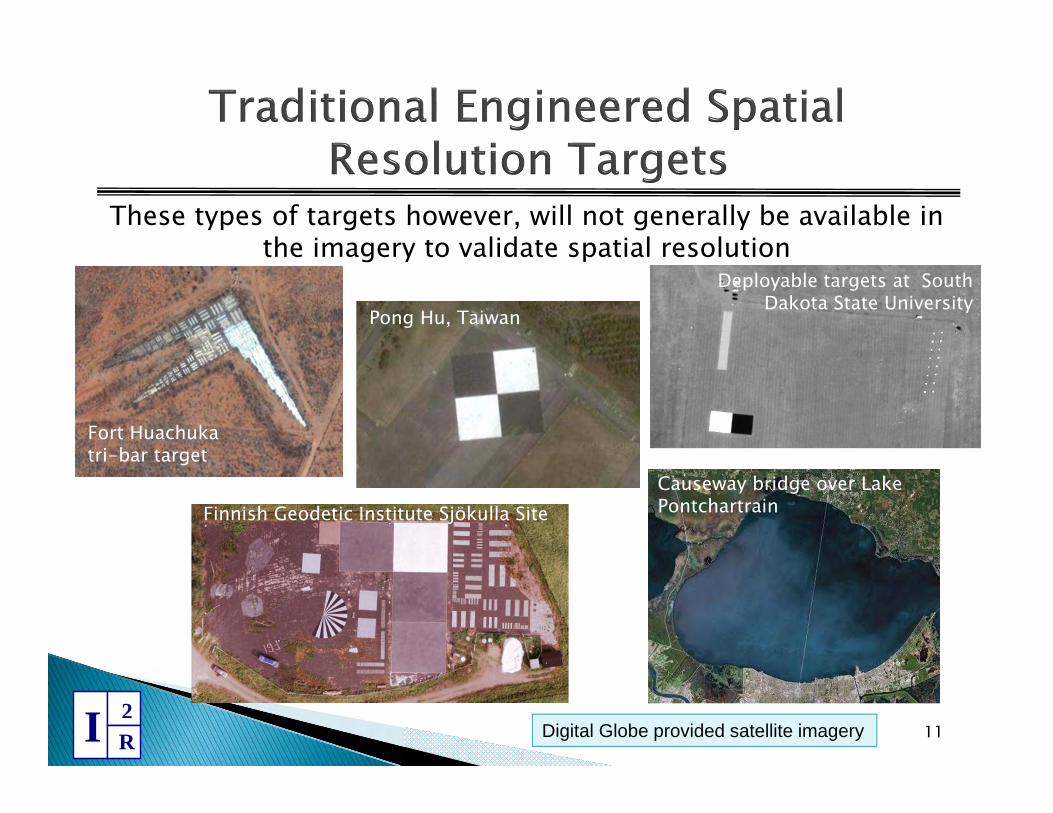
Fort Huachukatri-bar target
Deployable targets at South Dakota State University
Causeway bridge over Lake Pontchartrain
Digital Globe provided satellite imagery 11
Pong Hu, Taiwan
These types of targets however, will not generally be available in the imagery to validate spatial resolution
Finnish Geodetic Institute Sjökulla Site
I 2R
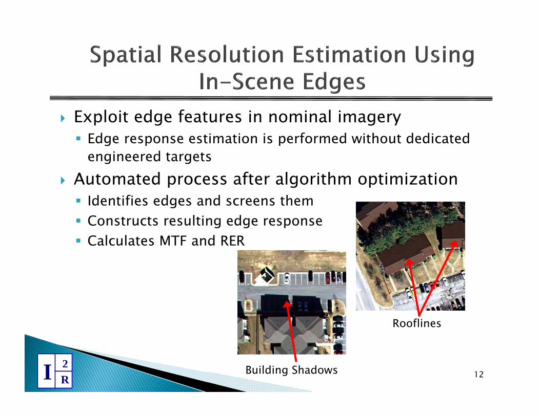
Exploit edge features in nominal imagery Edge response estimation is performed without dedicated
engineered targets Automated process after algorithm optimization Identifies edges and screens them Constructs resulting edge response Calculates MTF and RER
12Building Shadows
Rooflines
I 2R
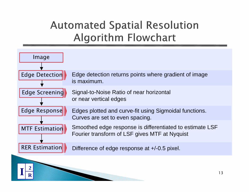
Image
Edge detection returns points where gradient of imageis maximum.
Signal-to-Noise Ratio of near horizontal or near vertical edges
Edges plotted and curve-fit using Sigmoidal functions.Curves are set to even spacing.
Smoothed edge response is differentiated to estimate LSFFourier transform of LSF gives MTF at Nyquist
Difference of edge response at +/-0.5 pixel.
Edge Detection
Edge ScreeningEdge Screening
Edge Response
MTF EstimationMTF Estimation
RER Estimation
13

I 2R
2 4 6 8 10 12 14 16
0
2
4
6
8
10
50 100 150 200 250 300
50
00
50
00
50
00
14
Satellite image: Digital Globe

I 2R 15
-8 -6 -4 -2 0 2 4 6-0.2
0
0.2
0.4
0.6
0.8
1
1.2
SNR = 40.57
Pixel
-8 -6 -4 -2 0 2 4 6-0.06
-0.04
-0.02
0
0.02
0.04
0.06
Pixel
-4 -3 -2 -1 0 1 2 3 40
0.2
0.4
0.6
0.8
1Normalized LSF
Cycles/Pixel
0 0.05 0.1 0.15 0.2 0.25 0.3 0.35 0.4 0.45 0.50
0.2
0.4
0.6
0.8
1MTF
Cycles/Pixel
Max DN = 783Min DN = 346
PixelsSigmoid
Residual FitSigmoid residuals
MTF
Normalized LSFEdge Response
Residuals

I 2R
Automated algorithm was validated using several years of IKONOS and QuickBird imagery of engineered targets by comparing automated algorithm results with traditional method
1
23
50 100 150 200 250 300
50
100
150
200
250
300
SSC Tarp Edge
Pulse Target Edge
16

I 2R
Automated algorithm reproduces results obtained using traditional approaches employing engineered targets GSD scales approx. 1 m Values combine cross track and in-track assessments
17
Sensor
MTF RER MTF RER
QuickBirdCC
0.14±0.04 0.52±0.03 0.13±0.03 0.53±0.03
IKONOSMTFC Off/CC
0.13±0.04 0.50±0.03 0.10±0.03 0.50±0.03
Traditional Method Automated Algorithm

I 2R
RapidEye sensors 5 bands in the visible-NIR blue (440-510), green (520-590), red (630-685),
red edge (690-730), NIR (760-850) IFOV GSD 6.5m and orthorectified resampled GSD 5m
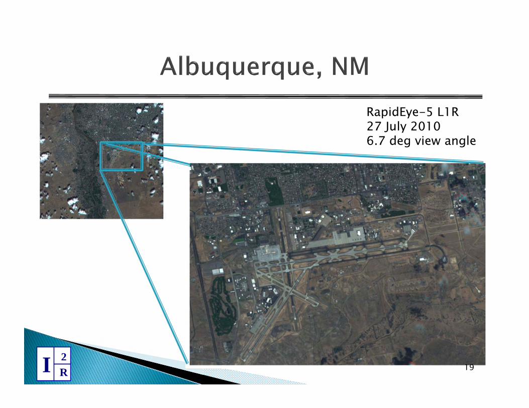
RapidEye provided I2R several Level1R scenes from RapidEye-5 (radiometrically corrected but not band aligned) Four Cities Albuquerque, NM Dallas Fort Worth, TX Nellis Air Force Base, NV Denver, CO
18
I 2R 19
RapidEye-5 L1R27 July 20106.7 deg view angle

I 2R
Automated edge detection Horizontal edge
20

I 2R
Edge Response Line Spread Function
Residuals MTF
21

I 2R 22
RapidEye-5 L1R22 June 20106.7 deg view angle

I 2R
Automated edge detection Vertical edge
23

I 2R
Edge Response Line Spread Function
Residuals MTF
24

I 2R 25
RapidEye-5 L1R15 August 20106.7 deg view angle

I 2R 26
RapidEye-5 L1R 04 May 2010Band 3 (red) 6.7 deg view angle

I 2R 27
Band Average MTF@ Nyquist 0.13 +/- 0.02
MTF STDNumEdges MTF STD
NumEdges MTF STD
NumEdges MTF STD
NumEdges
Band 1 0.12 0.09 46 0.12 0.07 132 0.12 0.06 68 0.16 0.09 45Band 2 0.11 0.06 45 0.12 0.06 132 0.13 0.09 70 0.15 0.08 43Band 3 0.12 0.09 45 0.14 0.06 131 0.12 0.06 79 0.14 0.07 52Band 4 0.11 0.07 45 0.15 0.07 131 0.13 0.07 91 0.15 0.08 52Band 5 0.13 0.09 46 0.15 0.07 128 0.17 0.08 135 0.14 0.07 62WeightedMean 0.12 0.03 0.14 0.03 0.13 0.03 0.15 0.03
Albequerque Dallas Denver Nellis
Level1R

I 2R 28
Band Average RER 0.54 +/- 0.02
RER STDNumEdges RER STD
NumEdges RER STD
NumEdges RER STD
NumEdges
Band 1 0.45 0.15 48 0.51 0.07 128 0.49 0.09 69 0.58 0.12 44Band 2 0.50 0.13 47 0.53 0.05 128 0.53 0.07 67 0.58 0.09 45Band 3 0.49 0.13 46 0.55 0.06 127 0.53 0.06 78 0.56 0.07 52Band 4 0.50 0.13 47 0.56 0.07 128 0.54 0.08 90 0.58 0.07 51Band 5 0.50 0.13 47 0.56 0.07 131 0.58 0.06 129 0.57 0.07 58WeightedMean 0.49 0.06 0.54 0.03 0.54 0.03 0.57 0.04
Albequerque Dallas Denver Nellis
Level1R

I 2R 29
Band Average MTF@ Nyquist 0.12 +/- 0.01
MTF STDNumEdges MTF STD
NumEdges MTF STD
NumEdges MTF STD
NumEdges
Band 1 0.06 0.05 16 0.18 0.09 145 0.10 0.05 73 0.15 0.08 37Band 2 0.07 0.06 16 0.16 0.08 147 0.11 0.06 75 0.14 0.07 38Band 3 0.14 0.09 33 0.17 0.08 146 0.12 0.06 75 0.14 0.04 37Band 4 0.16 0.09 33 0.17 0.08 145 0.12 0.06 100 0.14 0.06 38Band 5 0.13 0.08 32 0.15 0.07 145 0.11 0.06 104 0.10 0.05 36WeightedMean 0.09 0.03 0.16 0.04 0.11 0.03 0.13 0.02
Albequerque Dallas Denver Nellis
Level1R

I 2R 30
Band Average RER 0.52 +/- 0.02
RER STDNumEdges RER STD
NumEdges RER STD
NumEdges RER STD
NumEdges
Band 1 0.37 0.11 17 0.55 0.10 148 0.49 0.08 73 0.50 0.12 38Band 2 0.42 0.14 17 0.56 0.08 150 0.51 0.07 71 0.54 0.07 37Band 3 0.53 0.07 34 0.56 0.07 147 0.50 0.07 76 0.55 0.05 37Band 4 0.54 0.07 33 0.56 0.08 145 0.52 0.06 103 0.55 0.06 37Band 5 0.51 0.07 33 0.55 0.06 142 0.50 0.05 103 0.50 0.06 38WeightedMean 0.50 0.04 0.56 0.03 0.50 0.03 0.53 0.03
Albequerque Dallas Denver Nellis
Level1R
I 2R
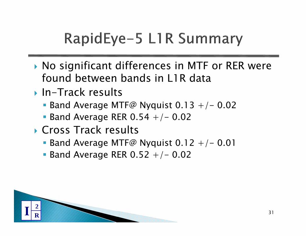
No significant differences in MTF or RER were found between bands in L1R data
In-Track results Band Average MTF@ Nyquist 0.13 +/- 0.02 Band Average RER 0.54 +/- 0.02
Cross Track results Band Average MTF@ Nyquist 0.12 +/- 0.01 Band Average RER 0.52 +/- 0.02
31
I 2R
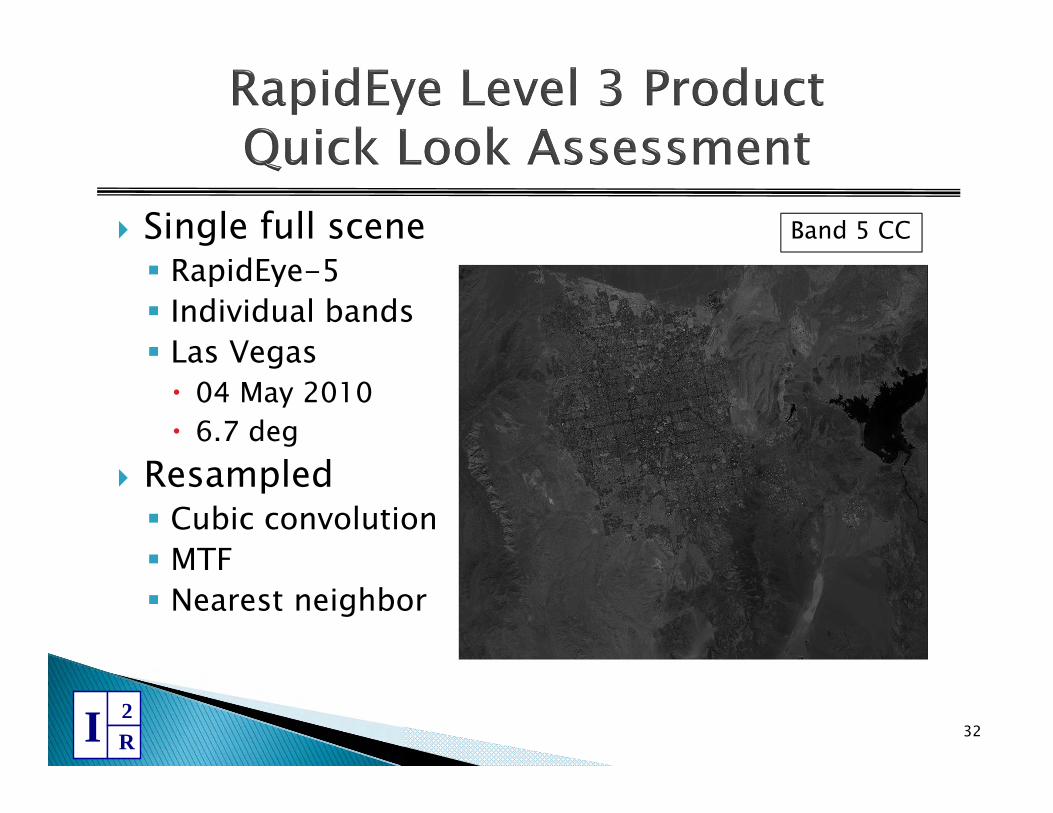
Single full scene RapidEye-5 Individual bands Las Vegas 04 May 2010 6.7 deg
Resampled Cubic convolution MTF Nearest neighbor
32
Band 5 CC
I 2R 33
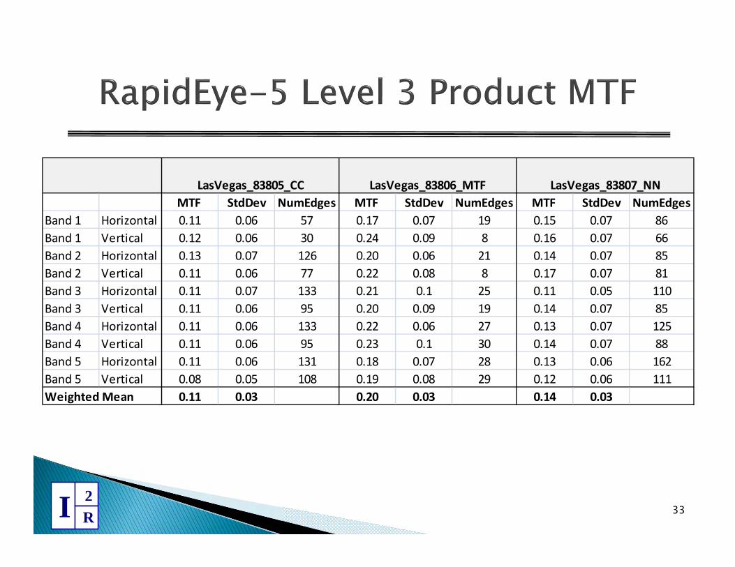
MTF StdDev NumEdges MTF StdDev NumEdges MTF StdDev NumEdgesBand 1 Horizontal 0.11 0.06 57 0.17 0.07 19 0.15 0.07 86Band 1 Vertical 0.12 0.06 30 0.24 0.09 8 0.16 0.07 66Band 2 Horizontal 0.13 0.07 126 0.20 0.06 21 0.14 0.07 85Band 2 Vertical 0.11 0.06 77 0.22 0.08 8 0.17 0.07 81Band 3 Horizontal 0.11 0.07 133 0.21 0.1 25 0.11 0.05 110Band 3 Vertical 0.11 0.06 95 0.20 0.09 19 0.14 0.07 85Band 4 Horizontal 0.11 0.06 133 0.22 0.06 27 0.13 0.07 125Band 4 Vertical 0.11 0.06 95 0.23 0.1 30 0.14 0.07 88Band 5 Horizontal 0.11 0.06 131 0.18 0.07 28 0.13 0.06 162Band 5 Vertical 0.08 0.05 108 0.19 0.08 29 0.12 0.06 111Weighted Mean 0.11 0.03 0.20 0.03 0.14 0.03
LasVegas_83805_CC LasVegas_83806_MTF LasVegas_83807_NN

I 2R 34
RER StdDev NumEdges RER StdDev NumEdges RER StdDev NumEdgesBand 1 Horizontal 0.54 0.07 59 0.60 0.05 18 0.56 0.07 85Band 1 Vertical 0.57 0.05 30 0.71 0.13 8 0.57 0.07 68Band 2 Horizontal 0.56 0.07 123 0.63 0.05 21 0.57 0.06 86Band 2 Vertical 0.54 0.06 77 0.67 0.06 8 0.58 0.06 81Band 3 Horizontal 0.53 0.06 133 0.64 0.07 25 0.54 0.05 108Band 3 Vertical 0.54 0.05 93 0.62 0.09 18 0.55 0.06 84Band 4 Horizontal 0.54 0.05 131 0.67 0.08 28 0.55 0.07 123Band 4 Vertical 0.53 0.05 96 0.64 0.08 30 0.55 0.06 88Band 5 Horizontal 0.54 0.06 133 0.63 0.08 28 0.55 0.06 160Band 5 Vertical 0.50 0.04 106 0.63 0.08 29 0.51 0.06 110Weighted Mean 0.54 0.02 0.64 0.04 0.55 0.03
LasVegas_83805_CC LasVegas_83806_MTF LasVegas_83807_NN

I 2R
Developed an automated engineering tool to estimate image quality parameters (MTF/RER) for high spatial resolution imagery Algorithm utilizes manmade edges found in normally acquired
urban imagery Successfully validated the tool using GeoEye IIKONOS and
Digital Globe QuickBird imagery by comparing results with that obtained using traditional methods
Tool must be optimized for each imaging system and requires engineering judgment
High quality results depend on statistical evaluation of hundreds of edges
35

I 2R
We are working at ways to further automate the tool so that it can be executed by those with less expertise
We are investigating ways to continually validate our tool using engineered targets and field teams
We are working with other satellite/aerial providers to estimate their image quality parameters…more to come
36