Embed Size (px)
Citation preview
Computational fluid dynamics
Martin [email protected]
Applied Scientific Computing (Tillämpad beräkningsvetenskap)
February 11, 2010
Martin Kronbichler (TDB) FVM for CFD February 11, 2010 1 / 72

Introduction
The Navier–Stokes equationsConservation of massConservation of momentum
Constitutive & kinematic relationsConservation of energyEquations of state & compressible Navier–Stokes equationsIncompressible Navier–Stokes equations
DiscretizationOverview of spatial discretizationsThe Finite Volume Method
Time discretizationSpatial discretization
Turbulence and its modeling
Martin Kronbichler (TDB) FVM for CFD February 11, 2010 2 / 72

Introduction
What is CFD?
I Fluid mechanics deals with the motion of fluids (liquids and gases),induced by external forces.
I Fluid flow is modeled by partial differential equations (PDE),describing the conservation of mass, momentum, and energy.
I Computational Fluid Dynamics (CFD) is the discipline ofdiscretizing these PDE and solving them using computers.
Martin Kronbichler (TDB) FVM for CFD February 11, 2010 3 / 72

Introduction
In which application fields is CFD used?
I Aerospace and aeronautical applications (airplanes, water and spacevehicles)
I Mechanical applications (gas turbines, heat exchange, explosions,combustion, architecture)
I Biological applications (blood flow, breathing, drinking)I Meteorological applications (weather prediction)I Environmental applications (air and water pollution)I and many more . . .
Martin Kronbichler (TDB) FVM for CFD February 11, 2010 4 / 72
Introduction
Why to use CFD?
I Pre-design of components: simulation vs. experiment (simulationsare cheaper, faster, and safer, but not always reliable)
I vehicles with lower fuel consumption, quieter, heavier loadsI combustion enginesI oil recoveryI water and gas turbines (effectiveness)I stress minimization
I Detection and predictionI hurricanes, storms, tsunamisI pollution transportI diseasesI forces, stresses
Martin Kronbichler (TDB) FVM for CFD February 11, 2010 5 / 72

Introduction
Visualization of CFD results
ONERA M6 wing optimizationO. Amoignon, M. Berggren
Martin Kronbichler (TDB) FVM for CFD February 11, 2010 6 / 72

Introduction
Visualization of CFD results
Pipe flow, computer lab
Martin Kronbichler (TDB) FVM for CFD February 11, 2010 7 / 72

Introduction
Requirements for industrial CFD
I Robustness — give a solution (for as many input cases as possible)I Reliability — give a good solutionI Performance — give a good solution fastI Geometries — give a good solution fast for real problemsI Automatic tool chain — reduce requirements of user interaction
Knowledgeable user controls and evaluates simulation outcomes!
Martin Kronbichler (TDB) FVM for CFD February 11, 2010 8 / 72

Introduction
CFD Solution Tool Chain
I CAD description of geometry
I Grid generation from CAD model (usually the most time consumingpart)
I Problem set up - knowledgeable user neededI Mathematical model to useI Spatial and temporal discretizationI Available resourcesI Much more . . .
I Preprocessing - parse configuration and prepare solverI Solving - run the solverI Post processing - extract and compute information of interestI Visualization - often most importantI Interpretation - physics, mathematics, numerics, experiments
Martin Kronbichler (TDB) FVM for CFD February 11, 2010 9 / 72

Introduction
CFD Solution Tool Chain
I CAD description of geometryI Grid generation from CAD model (usually the most time consuming
part)
I Problem set up - knowledgeable user neededI Mathematical model to useI Spatial and temporal discretizationI Available resourcesI Much more . . .
I Preprocessing - parse configuration and prepare solverI Solving - run the solverI Post processing - extract and compute information of interestI Visualization - often most importantI Interpretation - physics, mathematics, numerics, experiments
Martin Kronbichler (TDB) FVM for CFD February 11, 2010 9 / 72

Introduction
CFD Solution Tool Chain
I CAD description of geometryI Grid generation from CAD model (usually the most time consuming
part)I Problem set up - knowledgeable user needed
I Mathematical model to useI Spatial and temporal discretizationI Available resourcesI Much more . . .
I Preprocessing - parse configuration and prepare solver
I Solving - run the solverI Post processing - extract and compute information of interestI Visualization - often most importantI Interpretation - physics, mathematics, numerics, experiments
Martin Kronbichler (TDB) FVM for CFD February 11, 2010 9 / 72

Introduction
CFD Solution Tool Chain
I CAD description of geometryI Grid generation from CAD model (usually the most time consuming
part)I Problem set up - knowledgeable user needed
I Mathematical model to useI Spatial and temporal discretizationI Available resourcesI Much more . . .
I Preprocessing - parse configuration and prepare solverI Solving - run the solver
I Post processing - extract and compute information of interestI Visualization - often most importantI Interpretation - physics, mathematics, numerics, experiments
Martin Kronbichler (TDB) FVM for CFD February 11, 2010 9 / 72

Introduction
CFD Solution Tool Chain
I CAD description of geometryI Grid generation from CAD model (usually the most time consuming
part)I Problem set up - knowledgeable user needed
I Mathematical model to useI Spatial and temporal discretizationI Available resourcesI Much more . . .
I Preprocessing - parse configuration and prepare solverI Solving - run the solverI Post processing - extract and compute information of interest
I Visualization - often most importantI Interpretation - physics, mathematics, numerics, experiments
Martin Kronbichler (TDB) FVM for CFD February 11, 2010 9 / 72

Introduction
CFD Solution Tool Chain
I CAD description of geometryI Grid generation from CAD model (usually the most time consuming
part)I Problem set up - knowledgeable user needed
I Mathematical model to useI Spatial and temporal discretizationI Available resourcesI Much more . . .
I Preprocessing - parse configuration and prepare solverI Solving - run the solverI Post processing - extract and compute information of interestI Visualization - often most important
I Interpretation - physics, mathematics, numerics, experiments
Martin Kronbichler (TDB) FVM for CFD February 11, 2010 9 / 72

Introduction
CFD Solution Tool Chain
I CAD description of geometryI Grid generation from CAD model (usually the most time consuming
part)I Problem set up - knowledgeable user needed
I Mathematical model to useI Spatial and temporal discretizationI Available resourcesI Much more . . .
I Preprocessing - parse configuration and prepare solverI Solving - run the solverI Post processing - extract and compute information of interestI Visualization - often most importantI Interpretation - physics, mathematics, numerics, experiments
Martin Kronbichler (TDB) FVM for CFD February 11, 2010 9 / 72
Introduction
CFD software
I Commercial: Fluent, Comsol, CFX, Star-CDI In-house codes: Edge (FOI), DLR-Tau (German Aerospace Center),
Fun3D (NASA), Sierra/Premo (American Aerospace)I Open Source: OpenFOAM, FEniCS, OpenFlower
Martin Kronbichler (TDB) FVM for CFD February 11, 2010 10 / 72

Introduction
CFD links
I http://www.cfd-online.comI http://www.fluent.comI http://www.openfoam.org
Martin Kronbichler (TDB) FVM for CFD February 11, 2010 11 / 72

The Navier–Stokes equations
A mathematical model for fluid flow
The Navier–Stokes equations
Martin Kronbichler (TDB) FVM for CFD February 11, 2010 12 / 72

The Navier–Stokes equations
Navier–Stokes equations — an overview
I The governing equations of fluid dynamics are the conservation lawsof mass, momentum, and energy.
I In CFD, this set of conservation laws are called theNavier–Stokes equations.
I Derive compressible Navier–Stokes equations firstI Simplify these equations to get the incompressible Navier–Stokes
equations
Martin Kronbichler (TDB) FVM for CFD February 11, 2010 13 / 72

The Navier–Stokes equations
Notation
ρ densityu velocity, u = (u1, u2, u3)p pressureT temperatureµ dynamic viscosityν kinematic viscosity, ν = µ/ρ
∇ nabla operator, ∇ =(
∂∂x1 ,
∂∂x2 ,
∂∂x3
)· inner product, a · b = a1b1 + a2b2 + a3b3
Martin Kronbichler (TDB) FVM for CFD February 11, 2010 14 / 72

The Navier–Stokes equations
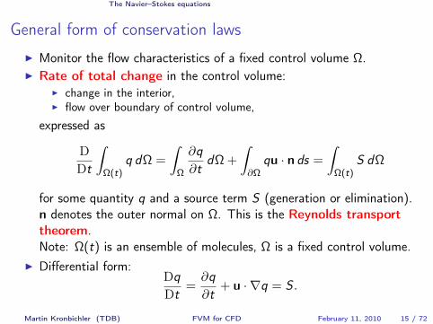
General form of conservation laws
I Monitor the flow characteristics of a fixed control volume Ω.I Rate of total change in the control volume:
I change in the interior,I flow over boundary of control volume,
expressed as
DDt
∫Ω(t)
q dΩ =
∫Ω
∂q∂t
dΩ +
∫∂Ω
qu · n ds =
∫Ω(t)
S dΩ
for some quantity q and a source term S (generation or elimination).n denotes the outer normal on Ω. This is the Reynolds transporttheorem.Note: Ω(t) is an ensemble of molecules, Ω is a fixed control volume.
I Differential form:DqDt
=∂q∂t
+ u · ∇q = S .
Martin Kronbichler (TDB) FVM for CFD February 11, 2010 15 / 72

The Navier–Stokes equations
General form of conservation laws
I Monitor the flow characteristics of a fixed control volume Ω.I Rate of total change in the control volume:
I change in the interior,I flow over boundary of control volume,
expressed as
DDt
∫Ω(t)
q dΩ =
∫Ω
∂q∂t
dΩ +
∫∂Ω
qu · n ds =
∫Ω(t)
S dΩ
for some quantity q and a source term S (generation or elimination).n denotes the outer normal on Ω. This is the Reynolds transporttheorem.Note: Ω(t) is an ensemble of molecules, Ω is a fixed control volume.
I Differential form:DqDt
=∂q∂t
+ u · ∇q = S .
Martin Kronbichler (TDB) FVM for CFD February 11, 2010 15 / 72

The Navier–Stokes equations Conservation of mass
Continuity equation I
The continuity equation describes the conservation of mass .
The massM of the material in Ω(t) is constant (molecules cannot becreated/destroyed), that isM(t) =M(t + ∆t).
DMDt
=DDt
∫Ω(t)
ρ dΩ︸ ︷︷ ︸M
= 0
ρ(t) denotes the fluid density.
Martin Kronbichler (TDB) FVM for CFD February 11, 2010 16 / 72
The Navier–Stokes equations Conservation of mass
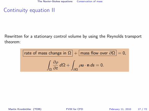
Continuity equation II
Rewritten for a stationary control volume by using the Reynolds transporttheorem:
rate of mass change in Ω + mass flow over ∂Ω = 0,∫Ω
∂ρ
∂tdΩ +
∫∂Ωρu · n ds = 0.
Martin Kronbichler (TDB) FVM for CFD February 11, 2010 17 / 72

The Navier–Stokes equations Conservation of momentum
Momentum equation I
The momentum equation describes the conservation of momentum .
Newton’s second law of motion: the total rate of momentum m change inΩ(t) is equal to the sum of acting forces K, i.e.,
DmDt
=DDt
∫Ω(t)
ρu dΩ = K,
(interpretation: mass × acceleration = force).
Martin Kronbichler (TDB) FVM for CFD February 11, 2010 18 / 72

The Navier–Stokes equations Conservation of momentum
Momentum equation II
Rewritten for a stationary control volume Ω:∫Ω
∂ρu∂t
+
∫∂Ωρ(u⊗ u) · n ds = K,
where u⊗ u is a rank-2 tensor with entries uiuj .
Decompose force into surface forces and volume forces:
rate of momentum change in Ω + momentum flow over ∂Ω
= surface forces on ∂Ω + volume forces on Ω ,∫Ω
∂ρu∂t
dV +
∫∂Ωρ(u⊗u)·n ds = −
∫∂Ω
pn ds +
∫∂Ωτ · n ds︸ ︷︷ ︸
surface forces
+
∫Ωρf dΩ.
Martin Kronbichler (TDB) FVM for CFD February 11, 2010 19 / 72

The Navier–Stokes equations Conservation of momentum
Momentum equation II
Rewritten for a stationary control volume Ω:∫Ω
∂ρu∂t
+
∫∂Ωρ(u⊗ u) · n ds = K,
where u⊗ u is a rank-2 tensor with entries uiuj .Decompose force into surface forces and volume forces:
rate of momentum change in Ω + momentum flow over ∂Ω
= surface forces on ∂Ω + volume forces on Ω ,∫Ω
∂ρu∂t
dV +
∫∂Ωρ(u⊗u)·n ds = −
∫∂Ω
pn ds +
∫∂Ωτ · n ds︸ ︷︷ ︸
surface forces
+
∫Ωρf dΩ.
Martin Kronbichler (TDB) FVM for CFD February 11, 2010 19 / 72

The Navier–Stokes equations Conservation of momentum
Momentum equation III
I Surface forces acting on ds of ∂Ω:I Pressure force p(−n) ds (analog to isotropic stress in structural
mechanics),I Viscous force τ · n ds, τ is the Cauchy stress tensor (analog to
deviatoric stress in structural mechanics).
I Volume forces ρf dΩ acting on small interior volume dΩ:I Gravity force ρg dΩ, e.g., f = g,I Other types of forces: Coriolis, centrifugal, electromagnetic, buoyancy
Martin Kronbichler (TDB) FVM for CFD February 11, 2010 20 / 72

The Navier–Stokes equations Conservation of momentum
Momentum equation III
I Surface forces acting on ds of ∂Ω:I Pressure force p(−n) ds (analog to isotropic stress in structural
mechanics),I Viscous force τ · n ds, τ is the Cauchy stress tensor (analog to
deviatoric stress in structural mechanics).I Volume forces ρf dΩ acting on small interior volume dΩ:
I Gravity force ρg dΩ, e.g., f = g,I Other types of forces: Coriolis, centrifugal, electromagnetic, buoyancy
Martin Kronbichler (TDB) FVM for CFD February 11, 2010 20 / 72

The Navier–Stokes equations Conservation of momentum
Newtonian fluidModel that relates the stress tensor τ to the velocity u:We consider so-called Newtonian fluids, where the viscous stress islinearly related to strain rate, that is,
τ = 2µε(u)− 23µI tr ε(u) = µ
(∇u + (∇u)T
)− 2
3µ(∇ · u)I,
(compare with constitutive and kinematic relations in elasticity theory).
For Cartesian coordinates
τij = µ
(∂uj
∂xi+∂ui
∂xj
)− 2
3µ
3∑k=1
∂uk
∂xk.
The dynamic viscosity is assumed constant
µ = µ(T , p) ≈ constant.
Martin Kronbichler (TDB) FVM for CFD February 11, 2010 21 / 72

The Navier–Stokes equations Conservation of energy
Energy equation I
The energy equation describes the conservation of energy .
The first law of thermodynamics:The total rate of total energy E changes in Ω(t) is equal to the rate ofwork L done on the fluid by the acting forces K plus the rate of heat addedW , that is
DEDt
=DDt
∫Ω(t)
ρE dΩ = L+ W
where ρE is the total energy per unit volume.
Martin Kronbichler (TDB) FVM for CFD February 11, 2010 22 / 72

The Navier–Stokes equations Conservation of energy
Energy Equation II
Rewritten for a stationary control volume Ω, explicitly specifying the sourceterms:
Rate of total energy change in Ω + Total energy flow over ∂Ω =
Rate of work of pressure and viscous forces on ∂Ω +
Rate of work of forces on Ω + Rate of heat added over ∂Ω∫Ω
∂ρE∂t
dΩ +
∫∂ΩρEu · n ds =−
∫∂Ω
pu · n ds +
∫∂Ω
(τ · u) · n ds
+
∫Ωρf · u dΩ +
∫∂Ω
k∇T · n ds
for the fluid temperature T and thermal conductivity k .
Martin Kronbichler (TDB) FVM for CFD February 11, 2010 23 / 72

The Navier–Stokes equations Conservation of energy
Involved variables and equations
We haveI seven variables (ρ, u1, u2, u3, p,T ,E )
I five equations (continuity, 3×momentum, energy)
We need two more equations to close the system, the so-called equationsof state.
Martin Kronbichler (TDB) FVM for CFD February 11, 2010 24 / 72

The Navier–Stokes equations Equations of state & compressible Navier–Stokes equations
Equations of state
Properties of a perfect gas:
p =(γ − 1)ρ
internal energy︷ ︸︸ ︷(E − 1
2|u|2)
T =1cv
(E − 1
2|u|2)
where γ =cpcv
is the ratio of specific heats, and cp and cv are the specificheats at constant pressure and volume.
A typical value for air at sea level pressure is γ = 1.4.
Martin Kronbichler (TDB) FVM for CFD February 11, 2010 25 / 72
The Navier–Stokes equations Equations of state & compressible Navier–Stokes equations
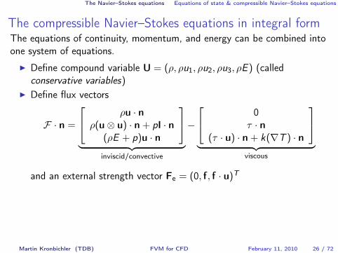
The compressible Navier–Stokes equations in integral formThe equations of continuity, momentum, and energy can be combined intoone system of equations.
I Define compound variable U = (ρ, ρu1, ρu2, ρu3, ρE ) (calledconservative variables)
I Define flux vectors
F · n =
ρu · nρ(u⊗ u) · n + pI · n
(ρE + p)u · n
︸ ︷︷ ︸
inviscid/convective
−
0τ · n
(τ · u) · n + k(∇T ) · n
︸ ︷︷ ︸
viscous
and an external strength vector Fe = (0, f, f · u)T
Compressible Navier–Stokes equations in integral form∫Ω
∂U∂t
dΩ +
∫∂ΩF · n ds =
∫ΩρFe dΩ
Martin Kronbichler (TDB) FVM for CFD February 11, 2010 26 / 72

The Navier–Stokes equations Equations of state & compressible Navier–Stokes equations
Compressible Navier–Stokes equations, differential form
Assume: flux tensor F is differentiable
Apply the Gauss theorem to the integral form and get∫Ω
(∂U∂t
+∇ · F − ρFe
)dΩ = 0.
Since the integral is zero for an arbitrary control volume Ω, we obtain thedifferential form of the
Compressible Navier–Stokes equations
∂U∂t
+∇ · F = ρFe .
Martin Kronbichler (TDB) FVM for CFD February 11, 2010 27 / 72

The Navier–Stokes equations Incompressible Navier–Stokes equations
The incompressible Navier–Stokes equations
Motivation: we can use simpler equations if we have more informationI Incompressible fluid: density does not change with pressure, i.e.,ρ = const.
I Energy equation decouples from the rest of the system; continuity andmomentum equations can be simplified.
I Many practically relevant flows are incompressible (e.g. air at speedsup to 100 m/s) — predominant CFD model
Martin Kronbichler (TDB) FVM for CFD February 11, 2010 28 / 72

The Navier–Stokes equations Incompressible Navier–Stokes equations
Continuity equation
The continuity equation,
∂ρ
∂t+∇ · (ρu) = 0,
becomes for constant ρ simply
∇ · u = 0, i.e.,3∑
i=1
∂ui
∂xi= 0.
Martin Kronbichler (TDB) FVM for CFD February 11, 2010 29 / 72
The Navier–Stokes equations Incompressible Navier–Stokes equations
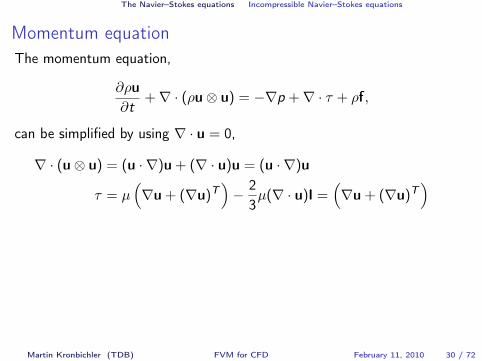
Momentum equationThe momentum equation,
∂ρu∂t
+∇ · (ρu⊗ u) = −∇p +∇ · τ + ρf,
can be simplified by using ∇ · u = 0,
∇ · (u⊗ u) = (u · ∇)u + (∇ · u)u = (u · ∇)u
τ = µ(∇u + (∇u)T
)− 2
3µ(∇ · u)I =
(∇u + (∇u)T
)
∇ · τ = µ∇ ·(∇u + (∇u)T
)= µ
(∇2u +∇(∇ · u)
)= µ∇2u.
This gives the incompressible version of the momentum equation
∂u∂t
+ (u · ∇)u = −1ρ∇p +
µ
ρ∇2u + f
Martin Kronbichler (TDB) FVM for CFD February 11, 2010 30 / 72

The Navier–Stokes equations Incompressible Navier–Stokes equations
Momentum equationThe momentum equation,
∂ρu∂t
+∇ · (ρu⊗ u) = −∇p +∇ · τ + ρf,
can be simplified by using ∇ · u = 0,
∇ · (u⊗ u) = (u · ∇)u + (∇ · u)u = (u · ∇)u
τ = µ(∇u + (∇u)T
)− 2
3µ(∇ · u)I =
(∇u + (∇u)T
)∇ · τ = µ∇ ·
(∇u + (∇u)T
)= µ
(∇2u +∇(∇ · u)
)= µ∇2u.
This gives the incompressible version of the momentum equation
∂u∂t
+ (u · ∇)u = −1ρ∇p +
µ
ρ∇2u + f
Martin Kronbichler (TDB) FVM for CFD February 11, 2010 30 / 72

The Navier–Stokes equations Incompressible Navier–Stokes equations
The incompressible Navier–Stokes equations II
Since the energy equation does not enter the momentum and continuityequation, we have a closed system of four equations:
Incompressible Navier–Stokes equations∇ · u = 0,∂u∂t
+ (u · ∇)u = −1ρ∇p + ν∇2u + f,
where ν = µρ is the fluid kinematic viscosity.
Martin Kronbichler (TDB) FVM for CFD February 11, 2010 31 / 72

The Navier–Stokes equations Incompressible Navier–Stokes equations
Equation in temperature
The energy equation can be expressed in terms of temperature by using theequation of state. Transforming the integral form into differential form asdone before1 yields
ρcp
[∂T∂t
+∇ · (Tu)
]= ∇ · (k∇T ) + τ : ∇u,
where
τ : ∇u =3∑
i ,j=1
τij∂uj
∂xi= µ
3∑i ,j=1
12
(∂ui
∂xj+∂uj
∂xi
)2
,
and is called a dissipative function.
1for further reading, see e.g. J. Blazek: Computational Fluid Dynamics, Elsevier,Amsterdam
Martin Kronbichler (TDB) FVM for CFD February 11, 2010 32 / 72

The Navier–Stokes equations Incompressible Navier–Stokes equations
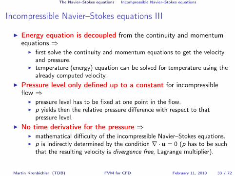
Incompressible Navier–Stokes equations III
I Energy equation is decoupled from the continuity and momentumequations ⇒
I first solve the continuity and momentum equations to get the velocityand pressure.
I temperature (energy) equation can be solved for temperature using thealready computed velocity.
I Pressure level only defined up to a constant for incompressibleflow ⇒
I pressure level has to be fixed at one point in the flow.I p yields then the relative pressure difference with respect to that
pressure level.I No time derivative for the pressure ⇒
I mathematical difficulty of the incompressible Navier–Stokes equations.I p is indirectly determined by the condition ∇ · u = 0 (p has to be such
that the resulting velocity is divergence free, Lagrange multiplier).
Martin Kronbichler (TDB) FVM for CFD February 11, 2010 33 / 72

The Navier–Stokes equations Incompressible Navier–Stokes equations
Incompressible Navier–Stokes equations III
I Energy equation is decoupled from the continuity and momentumequations ⇒
I first solve the continuity and momentum equations to get the velocityand pressure.
I temperature (energy) equation can be solved for temperature using thealready computed velocity.
I Pressure level only defined up to a constant for incompressibleflow ⇒
I pressure level has to be fixed at one point in the flow.I p yields then the relative pressure difference with respect to that
pressure level.
I No time derivative for the pressure ⇒I mathematical difficulty of the incompressible Navier–Stokes equations.I p is indirectly determined by the condition ∇ · u = 0 (p has to be such
that the resulting velocity is divergence free, Lagrange multiplier).
Martin Kronbichler (TDB) FVM for CFD February 11, 2010 33 / 72
The Navier–Stokes equations Incompressible Navier–Stokes equations
Incompressible Navier–Stokes equations III
I Energy equation is decoupled from the continuity and momentumequations ⇒
I first solve the continuity and momentum equations to get the velocityand pressure.
I temperature (energy) equation can be solved for temperature using thealready computed velocity.
I Pressure level only defined up to a constant for incompressibleflow ⇒
I pressure level has to be fixed at one point in the flow.I p yields then the relative pressure difference with respect to that
pressure level.I No time derivative for the pressure ⇒
I mathematical difficulty of the incompressible Navier–Stokes equations.I p is indirectly determined by the condition ∇ · u = 0 (p has to be such
that the resulting velocity is divergence free, Lagrange multiplier).
Martin Kronbichler (TDB) FVM for CFD February 11, 2010 33 / 72

The Navier–Stokes equations Incompressible Navier–Stokes equations
Additional conditions
To complete the physical problem setup after having derived theappropriate PDE, we have to define the
I domainI initial conditions (velocity, temperature, etc at t = 0)I boundary conditions (inflow, outflow, wall, interface, . . .)I material properties
Martin Kronbichler (TDB) FVM for CFD February 11, 2010 34 / 72

Discretization
Discretization
Numerical solution strategies for theflow equations
Martin Kronbichler (TDB) FVM for CFD February 11, 2010 35 / 72

Discretization
Solution Strategies Outline
Some points we will cover regarding solver strategies of CFDI Pros and cons of various discretization methodsI Finite Volume Method (FVM)I Turbulence and its modeling
Martin Kronbichler (TDB) FVM for CFD February 11, 2010 36 / 72

Discretization Overview of spatial discretizations
Overview of Methods
Discretization methods for the CFD equations:I Finite Difference Method (FDM)
+ efficiency, + theory, − geometriesI Finite Element Method (FEM)
+ theory, + geometries, − shocks, − uses no directional informationI Spectral Methods (Collocation, Galerkin, . . .)
+ accuracy, + theory, − geometries
I Finite Volume Methods (FVM)+ robustness, + geometries, − accuracy
I Discontinuous Galerkin Methods (DGM)+ geometries, + shocks, − efficiency (e.g. smooth solutions)
I Hybrid Methods+ versatile, − complex (not automatable)
Martin Kronbichler (TDB) FVM for CFD February 11, 2010 37 / 72

Discretization Overview of spatial discretizations
Overview of Methods
Discretization methods for the CFD equations:I Finite Difference Method (FDM)
+ efficiency, + theory, − geometriesI Finite Element Method (FEM)
+ theory, + geometries, − shocks, − uses no directional informationI Spectral Methods (Collocation, Galerkin, . . .)
+ accuracy, + theory, − geometriesI Finite Volume Methods (FVM)
+ robustness, + geometries, − accuracyI Discontinuous Galerkin Methods (DGM)
+ geometries, + shocks, − efficiency (e.g. smooth solutions)
I Hybrid Methods+ versatile, − complex (not automatable)
Martin Kronbichler (TDB) FVM for CFD February 11, 2010 37 / 72

Discretization Overview of spatial discretizations
Overview of Methods
Discretization methods for the CFD equations:I Finite Difference Method (FDM)
+ efficiency, + theory, − geometriesI Finite Element Method (FEM)
+ theory, + geometries, − shocks, − uses no directional informationI Spectral Methods (Collocation, Galerkin, . . .)
+ accuracy, + theory, − geometriesI Finite Volume Methods (FVM)
+ robustness, + geometries, − accuracyI Discontinuous Galerkin Methods (DGM)
+ geometries, + shocks, − efficiency (e.g. smooth solutions)I Hybrid Methods
+ versatile, − complex (not automatable)
Martin Kronbichler (TDB) FVM for CFD February 11, 2010 37 / 72

Discretization The Finite Volume Method
Introduction
The Finite Volume Method (FVM) is based on the integral form of thegoverning equations.
The integral conservation is enforced in so-called control volumes( dΩ→ ∆Ω) defined by the computational mesh.
The type of FVM is specified byI the type of control volumeI the type of evaluation of integrals and fluxes
Martin Kronbichler (TDB) FVM for CFD February 11, 2010 38 / 72

Discretization The Finite Volume Method
FVM derivation, introduction
Consider a general scalar hyperbolic conservation law:
∂u∂t
+∇ · F(u) = 0 in Ω, (1)
with appropriate boundary and initial conditions.
Compared to the compressible Navier–Stokes equations, we use a problemwhere
I u replaces the vector of conservative variables (ρ, ρu, ρE ),I F replaces the flux tensor as defined earlier,I we have a scalar problem instead of a system.
Martin Kronbichler (TDB) FVM for CFD February 11, 2010 39 / 72

Discretization The Finite Volume Method
FVM derivation, control volumes
Consider the equation in two dimensions, and we divide the domain Ω intoM non-overlapping control volumes Km ⊂ Ω.
Km
vertex-centered finite volume method
Martin Kronbichler (TDB) FVM for CFD February 11, 2010 40 / 72

Discretization The Finite Volume Method
FVM derivation, discretized solution
In each control volume, Km, we store one value um, which is the averageof u in Km.
um =1|Km|
∫Km
u dΩ
Martin Kronbichler (TDB) FVM for CFD February 11, 2010 41 / 72
Discretization The Finite Volume Method
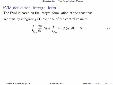
FVM derivation, integral form IThe FVM is based on the integral formulation of the equations.
We start by integrating (1) over one of the control volumes,∫Km
∂u∂t
dΩ +
∫Km
∇ · F(u) dΩ = 0. (2)
The first integral can be simplified by changing order of time derivative andintegration to get∫
Km
∂u∂t
dΩ =ddt
∫Km
u dΩ = |Km|dum
dt. (3)
Inserting (3) back into (2) yields
dum
dt= − 1|Km|
∫Km
∇ · F(u) dΩ.
Martin Kronbichler (TDB) FVM for CFD February 11, 2010 42 / 72

Discretization The Finite Volume Method
FVM derivation, integral form IThe FVM is based on the integral formulation of the equations.
We start by integrating (1) over one of the control volumes,∫Km
∂u∂t
dΩ +
∫Km
∇ · F(u) dΩ = 0. (2)
The first integral can be simplified by changing order of time derivative andintegration to get∫
Km
∂u∂t
dΩ =ddt
∫Km
u dΩ = |Km|dum
dt. (3)
Inserting (3) back into (2) yields
dum
dt= − 1|Km|
∫Km
∇ · F(u) dΩ.
Martin Kronbichler (TDB) FVM for CFD February 11, 2010 42 / 72
Discretization The Finite Volume Method
FVM derivation, time evolution
We need to propagate the solution um in time.
There are many possibilities for choosing a time integration method, forexample Runge–Kutta, multistep methods etc.
See some Ordinary Differential Equation (ODE) textbook for moreinformation.2
We will use forward Euler in all our examples, i.e.,
dum
dt=
un+1m − un
m∆t
,
where unm = um(tn).
2e.g., E. Hairer, S.P. Nørsett, G. Wanner: Solving Ordinary Differential Equations. I:Nonstiff Problems. Springer-Verlag, Berlin, 1993.
Martin Kronbichler (TDB) FVM for CFD February 11, 2010 43 / 72

Discretization The Finite Volume Method
FVM derivation, time evolution
Inserting the forward Euler time discretization into our system gives
un+1m = un
m −∆t|Km|
∫Km
∇ · F(u) dΩ.
Martin Kronbichler (TDB) FVM for CFD February 11, 2010 44 / 72

Discretization The Finite Volume Method
FVM derivation, integral form II
By integration by parts (Gauss divergence theorem) of the flux integral weget the basic FVM formulation
un+1m = un
m −∆t|Km|
∫∂Km
F(u) · n ds. (4)
The boundary integral describes the flux of u over the boundary ∂Km ofthe control volume.
Note: Transforming the volume to a surface integral gets us back to theform used for the derivation of the Navier–Stokes equations.
Different ways of evaluating the flux integral specify the type of FVM(together with the control volume type).
Martin Kronbichler (TDB) FVM for CFD February 11, 2010 45 / 72

Discretization The Finite Volume Method
FVM derivation, numerical flux
The integral in (4) is evaluated using a so-called numerical flux function.I There are a lot of different numerical fluxes available for the integral
evaluation, each of them having its pros and cons.Terminology: Riemann solvers (they are usually designed to solve theRiemann problem which is a conservation law with constant data anda discontinuity).
I Both exact and approximate solvers (i.e., ways to evaluate the fluxintegral (4)) have been developed, usually the latter class is used.
I E.g. exact solver for Euler3 equations developed by Godunov.I Widely used approximate solvers: Roe, HLLC, central flux.
3Contains only the inviscid terms from the compressible Navier–Stokes equationsMartin Kronbichler (TDB) FVM for CFD February 11, 2010 46 / 72
Discretization The Finite Volume Method
FVM derivation, numerical flux II
The numerical flux functions are usually denoted by F∗(uL, uR ,n) where uLis the left (local) state and uR is the right (remote) state of u at theboundary ∂Km, ∫
∂Km
F(u) · n ds =∑
j
∫∂K j
m
F(u) · nj ds
≈∑
j
|∂K jm|F∗(uL, uR ,nj)
and j denotes the index of each subboundary of ∂Km with a given normalnj .
Martin Kronbichler (TDB) FVM for CFD February 11, 2010 47 / 72

Discretization The Finite Volume Method
FVM derivation, full discretization
The full discretization for control volume Km is hence
un+1m = un
m −∆t|Km|
∑j
|∂K jm|F∗(uL, uR ,nj)
In one dimension, we have
un+1m = un
m −∆t∆x
∫∂Km
F(u) · n ds
= unm −
∆t∆x
(F(un
m+1/2)−F(unm−1/2)
)= un
m −∆t∆x
(F∗(un
m, unm−1,−1) + F∗(un
m, unm+1, 1)
)
Martin Kronbichler (TDB) FVM for CFD February 11, 2010 48 / 72

Discretization The Finite Volume Method
FVM derivation, full discretization
The full discretization for control volume Km is hence
un+1m = un
m −∆t|Km|
∑j
|∂K jm|F∗(uL, uR ,nj)
In one dimension, we have
un+1m = un
m −∆t∆x
∫∂Km
F(u) · n ds
= unm −
∆t∆x
(F(un
m+1/2)−F(unm−1/2)
)
= unm −
∆t∆x
(F∗(un
m, unm−1,−1) + F∗(un
m, unm+1, 1)
)
Martin Kronbichler (TDB) FVM for CFD February 11, 2010 48 / 72

Discretization The Finite Volume Method
FVM derivation, full discretization
The full discretization for control volume Km is hence
un+1m = un
m −∆t|Km|
∑j
|∂K jm|F∗(uL, uR ,nj)
In one dimension, we have
un+1m = un
m −∆t∆x
∫∂Km
F(u) · n ds
= unm −
∆t∆x
(F(un
m+1/2)−F(unm−1/2)
)= un
m −∆t∆x
(F∗(un
m, unm−1,−1) + F∗(un
m, unm+1, 1)
)
Martin Kronbichler (TDB) FVM for CFD February 11, 2010 48 / 72

Discretization The Finite Volume Method
FVM derivation, upwind scheme I
Get the information upwind, where the information comes from.
Image from http://en.wikipedia.org
Martin Kronbichler (TDB) FVM for CFD February 11, 2010 49 / 72

Discretization The Finite Volume Method
FVM derivation, upwind scheme IIExample in one dimension
F(u) = βu,
where β is the direction of the flow. So in each control volume we compute∫∂Km
βun ds.
Case β > 0 (information flows from left to right), equidistant mesh:
um−1/2 = um−1, um+1/2 = um.
Hence, we get
un+1m = un
m −∆t∆x
(F(un
m+1/2)nm+1/2 + F(unm−1/2)nm−1/2
)= un
m −∆t∆x
β(unm+1/2 − un
m−1/2
)= un
m −∆t∆x
β(unm − un
m−1).
Martin Kronbichler (TDB) FVM for CFD February 11, 2010 50 / 72

Discretization The Finite Volume Method
FVM derivation, upwind scheme (Roe flux)
Practical implementation of upwinding: construct it by the Roe Flux
F∗(uL, uR ,n) =n · F(uL) + n · F(uR)
2+∣∣n · F ′(u)
∣∣ uL − uR
2.
Here, u satisfies the mean value theorem,
n · F(uL) = n · F(uR) + n · F ′(u) (uL − uR) .
and is called the Roe average (problem dependent).
Upwinding is first order accurate.
Martin Kronbichler (TDB) FVM for CFD February 11, 2010 51 / 72
Discretization The Finite Volume Method
FVM derivation, central scheme I
For F(u) = βu on a equidistant mesh, the central scheme approximation is
um−1/2 =um−1 + um
2, um−1/2 =
um + um+1
2.
Hence,
un+1m = un
m −∆t∆x
(F(un
m+1/2)nm+1/2 + F(unm−1/2)nm−1/2
)= un
m −∆t∆x
β(unm+1/2 − un
m−1/2
)= un
m −∆t∆x
β
(unm + un
m+1
2−
unm−1 + un
m
2
)= un
m −∆t∆x
β
(unm+1 − un
m−12
).
Martin Kronbichler (TDB) FVM for CFD February 11, 2010 52 / 72

Discretization The Finite Volume Method
FVM derivation, central scheme II
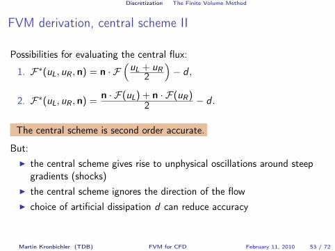
Possibilities for evaluating the central flux:
1. F∗(uL, uR ,n) = n · F(uL + uR
2
)− d ,
2. F∗(uL, uR ,n) =n · F(uL) + n · F(uR)
2 − d .
The central scheme is second order accurate.
But:I the central scheme gives rise to unphysical oscillations around steep
gradients (shocks)I the central scheme ignores the direction of the flowI choice of artificial dissipation d can reduce accuracy
Martin Kronbichler (TDB) FVM for CFD February 11, 2010 53 / 72
Discretization The Finite Volume Method
FVM derivation, central scheme II
Possibilities for evaluating the central flux:
1. F∗(uL, uR ,n) = n · F(uL + uR
2
)− d ,
2. F∗(uL, uR ,n) =n · F(uL) + n · F(uR)
2 − d .
The central scheme is second order accurate.
But:I the central scheme gives rise to unphysical oscillations around steep
gradients (shocks)I the central scheme ignores the direction of the flowI choice of artificial dissipation d can reduce accuracy
Martin Kronbichler (TDB) FVM for CFD February 11, 2010 53 / 72

Discretization The Finite Volume Method
FVM derivation, second derivatives
Flux tensor F contains terms with first derivatives in u for theNavier–Stokes equations (corresponding to second derivatives in thedifferential form of the equations).
Need to approximate these terms before evaluating the flux function.
Usually, apply central differences of the kind(∂u∂x
)m−1/2
=um − um−1
∆x.
Martin Kronbichler (TDB) FVM for CFD February 11, 2010 54 / 72

Discretization The Finite Volume Method
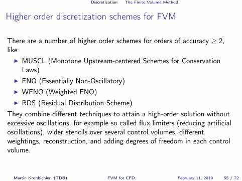
Higher order discretization schemes for FVM
There are a number of higher order schemes for orders of accuracy ≥ 2,like
I MUSCL (Monotone Upstream-centered Schemes for ConservationLaws)
I ENO (Essentially Non-Oscillatory)I WENO (Weighted ENO)I RDS (Residual Distribution Scheme)
They combine different techniques to attain a high-order solution withoutexcessive oscillations, for example so called flux limiters (reducing artificialoscillations), wider stencils over several control volumes, differentweightings, reconstruction, and adding degrees of freedom in each controlvolume.
Martin Kronbichler (TDB) FVM for CFD February 11, 2010 55 / 72
Discretization The Finite Volume Method
Higher order discretization schemes for FVM
There are a number of higher order schemes for orders of accuracy ≥ 2,like
I MUSCL (Monotone Upstream-centered Schemes for ConservationLaws)
I ENO (Essentially Non-Oscillatory)I WENO (Weighted ENO)I RDS (Residual Distribution Scheme)
They combine different techniques to attain a high-order solution withoutexcessive oscillations, for example so called flux limiters (reducing artificialoscillations), wider stencils over several control volumes, differentweightings, reconstruction, and adding degrees of freedom in each controlvolume.
Martin Kronbichler (TDB) FVM for CFD February 11, 2010 55 / 72

Discretization The Finite Volume Method
Choosing the discretization parameters
A necessary condition for stability of the time discretization is the CFLcondition (depends on the combination of space and time discretization).
For the one dimensional upwind discretization
un+1m = un
m −∆t∆x
β(unm − un
m−1),
we require ∣∣∣∣∆t∆x
β
∣∣∣∣ ≤ 1.
Interpretation: The difference approximation (which only uses informationfrom one grid point to the left/right) can only represent variations in thesolution up to β/∆x from one time step to the next → time step size hasto be smaller than that limit
Martin Kronbichler (TDB) FVM for CFD February 11, 2010 56 / 72

Discretization The Finite Volume Method
Steady state calculationsFor certain computations, the time-dependance is of no importance.
Sought: steady state solution. when the solution has stabilized, thechange in time will go to zero,
un+1m = un
m −∆t|Km|
∑j
|∂K jm|F∗(uL, uR ,nj)︸ ︷︷ ︸
residual
= unm, ∀m.
Measure whether steady state has been achieved: residual gets small.
To reach steady state, many different acceleration techniques can be used,for example local time stepping and multigrid.
Two examples of steady state:I computation of the drag and lift around an airfoil,I mixing problem considered in the computer lab.
Martin Kronbichler (TDB) FVM for CFD February 11, 2010 57 / 72

Discretization The Finite Volume Method
FVM for the incompressible Navier–Stokes equations
I The incompressible Navier–Stokes equations are a system in fiveequations (u, p,T ), so go through them one by one according to theabove procedure
I Need to take special care of p, since it does not involve a timederivative
I Computational domain Ω and material parameters ρ, ν specified fromapplication
I Initial and boundary conditions complete the formulation
Martin Kronbichler (TDB) FVM for CFD February 11, 2010 58 / 72

Discretization The Finite Volume Method
Initial condition
The state of all variables at time t0 has to be defined in order to initiatethe solution process.For example
u|t=0 = u0.
Martin Kronbichler (TDB) FVM for CFD February 11, 2010 59 / 72

Discretization The Finite Volume Method
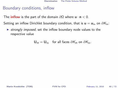
Boundary conditions, inflow
The inflow is the part of the domain ∂Ω where u · n < 0.
Setting an inflow Dirichlet boundary condition, that is u = uin on ∂Kin:
I strongly imposed, set the inflow boundary node values to therespective value
Um = Uin for all faces ∂Km on ∂Kin.
I weakly imposed, use the numerical flux,
F∗(Um,Uin,n).
The inflow data can be viewed as given in a ghost point; boundarytreated as the interior.
Martin Kronbichler (TDB) FVM for CFD February 11, 2010 60 / 72
Discretization The Finite Volume Method
Boundary conditions, inflow
The inflow is the part of the domain ∂Ω where u · n < 0.
Setting an inflow Dirichlet boundary condition, that is u = uin on ∂Kin:
I strongly imposed, set the inflow boundary node values to therespective value
Um = Uin for all faces ∂Km on ∂Kin.
I weakly imposed, use the numerical flux,
F∗(Um,Uin,n).
The inflow data can be viewed as given in a ghost point; boundarytreated as the interior.
Martin Kronbichler (TDB) FVM for CFD February 11, 2010 60 / 72

Discretization The Finite Volume Method
Boundary conditions, outflow
The outflow is the part of the domain ∂Ω where u · n > 0.Treating outflow boundaries is more complicated than inflow parts.
Usually one does a weak formulation such that1. F∗(UL,UL,n) is used as flux function,2. F∗(UL,U∞,n) is used as flux function with U∞ a far-field
velocity/pressure/temperature.There are also strong formulations.
Beware of artificial back flows!
A common trick is to make the domain big enough to avoid distorting thesolution in the domain of interest.
Martin Kronbichler (TDB) FVM for CFD February 11, 2010 61 / 72

Discretization The Finite Volume Method
Boundary conditions, solid walls
The solid wall is the part of the domain ∂Ω where u · n = 0.For viscous (Navier–Stokes) flow we apply a no-slip condition
u = 0.
These boundary conditions are usually imposed strongly.
Martin Kronbichler (TDB) FVM for CFD February 11, 2010 62 / 72

Discretization The Finite Volume Method
Heat transfer
When considering heat transfer for the incompressible Navier–Stokesequations, we also need to assign a BC for the temperature T . Twomechanisms can be applied:
I specify temperature with a Dirichlet BC, T = Tw , orI specify heat flux with a Neumann BC, ∂T/∂n = −fq/κ.
Martin Kronbichler (TDB) FVM for CFD February 11, 2010 63 / 72

Discretization The Finite Volume Method
Turbulence
Turbulence
Martin Kronbichler (TDB) FVM for CFD February 11, 2010 64 / 72

Turbulence and its modeling
Introduction, dimensionless form
In CFD, a scaled dimensionless form of the Navier–Stokes equation is oftenused.
We introduce new variables
x∗i =xi
L, u∗i =
ui
U, p∗ =
pU2ρ
,∂
∂xi=
1L∂
∂x∗i,
∂
∂t=
UL∂
∂t∗,
in which the incompressible Navier–Stokes equations read
∇∗ · u∗ = 0,∂u∗
∂t∗+ (u∗ · ∇∗)u∗ = −∇∗p∗ +
ν
UL︸︷︷︸Re−1
∇2u∗.
Martin Kronbichler (TDB) FVM for CFD February 11, 2010 65 / 72

Turbulence and its modeling
Reynolds number and turbulence
The Reynolds number is defined as
Re =ULν
=Inertial forcesViscous forces
,
where U, L, ν are the characteristic velocity, characteristic length, and thekinematic viscosity, respectively.
Fluids with the same Reynolds number behave the same way.
When the Reynolds number becomes larger than a critical value, theformerly laminar flow changes into turbulent flow, for example atRe ≈ 2300 for pipe flows.
Martin Kronbichler (TDB) FVM for CFD February 11, 2010 66 / 72

Turbulence and its modeling
Characterization of turbulence
Turbulent flows areI time dependentI three dimensionalI irregularI vortical (ω = ∇× u)
Image from http://en.wikipedia.org
Describing the turbulence can be done in many ways, and the choice of themethod depends on the application at hand and on computationalresources.
Martin Kronbichler (TDB) FVM for CFD February 11, 2010 67 / 72

Turbulence and its modeling
Direct Numerical Simulation (DNS)
I All scales in space and time are resolved.I No modeling of the turbulence.I Limited to small Reynolds numbers, because extremely fine grids and
time steps are required, O(Re3) spatial and temporal degrees offreedom.
Applications of DNS:I Turbulence research.I Reference results to verify other turbulence models.
Martin Kronbichler (TDB) FVM for CFD February 11, 2010 68 / 72

Turbulence and its modeling
Large Eddie Simulation (LES)
Only the large scales are resolved, and small scales are modeled.
Active research.
LES quite popular in certain industries, but still very costly.
Martin Kronbichler (TDB) FVM for CFD February 11, 2010 69 / 72

Turbulence and its modeling
Reynolds-Averaged Navier–Stokes (RANS) I
Concept introduced by Reynolds in 1895. The most commonly usedapproach in industry. Only time averages are considered, nonlinear effectsof the fluctuations are modeled.
Use the decomposition
u(x, t) = u(x, t)︸ ︷︷ ︸time average
+ u′(x, t)︸ ︷︷ ︸fluctuation
,
where the time average is
u(x, t) =1δ
∫ t+δ
tu(x, τ) dτ,
(spatial averaging or ensemble averaging can otherwise be used).
Martin Kronbichler (TDB) FVM for CFD February 11, 2010 70 / 72
Turbulence and its modeling
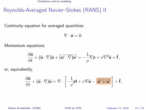
Reynolds-Averaged Navier–Stokes (RANS) II
Continuity equation for averaged quantities:
∇ · u = 0.
Momentum equations:
∂u∂t
+ (u · ∇)u + (u′ · ∇)u′ = −1ρ∇p + ν∇2u + f,
or, equivalently,
∂u∂t
+ (u · ∇)u = ∇ ·[−1ρpI + ν∇u− u′ ⊗ u′
]+ f,
Martin Kronbichler (TDB) FVM for CFD February 11, 2010 71 / 72
Turbulence and its modeling
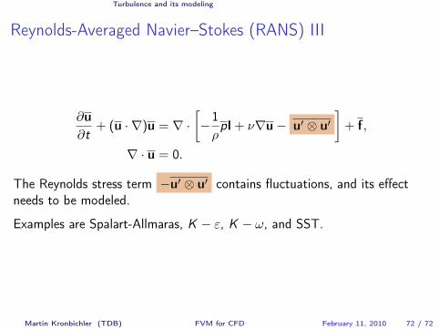
Reynolds-Averaged Navier–Stokes (RANS) III
∂u∂t
+ (u · ∇)u = ∇ ·[−1ρpI + ν∇u− u′ ⊗ u′
]+ f,
∇ · u = 0.
The Reynolds stress term −u′ ⊗ u′ contains fluctuations, and its effectneeds to be modeled.
Examples are Spalart-Allmaras, K − ε, K − ω, and SST.
Martin Kronbichler (TDB) FVM for CFD February 11, 2010 72 / 72