Martingale calculus and a maximal inequality forsupermartingales

B. Hajek

Department of Electrical and Computer Engineeringand the Coordinated Science Laboratory

University of Illinois at Urbana-Champaign

March 15, 2010

Abstract:

In the first hour of this two part presentation, the calculus ofsemimartingales, which includes martingales with both continuousand discrete components, will be reviewed. In the second hour ofthe presentation, a tight upper bound is given involving themaximum of a supermartingale. Specifically, it is shown that if Y isa semimartingale with initial value zero and quadratic variationprocess [Y,Y] such that Y + [Y,Y] is a supermartingale, then theprobability the maximum of Y is greater than or equal to a positiveconstant a is less than or equal to 1/(1+a). The proof uses thesemimartingale calculus and is inspired by dynamic programming.If Y has stationary independent increments, the bounds of J.F.C.Kingman apply to this situation. Complements and extensions willalso be given. (Preliminary paper posted to AirXiv:http://arxiv.org/abs/0911.4444).

Outline

Brief review of martingale calculus

Kingman’s moment bound

Bound on maximum of a supermartingale (with no SII assumption)

The big jump construction

Proof of the upper bound

Discrete time, version I

Discrete time, version II

A lemma

Comparison to Doob’s moment bounds

PART I: Brief review of martingale calculus

See, for example, [4, 5, 7, 8, 9] for more detail.

The usual underlying conditions

I Assume (Ω,F ,P) is complete (subsets of events withprobability zero are events)

I Assume filtration of σ-algebras F• = (Ft : t ≥ 0) isI right-continuous, andI each Ft includes all zero-probability events.

I Thus martingales, supermartingales, and submartingales havecadlag (right continuous with finite left limits) versions. Weassume in these slides such versions are used, without furtherexplicit mention.

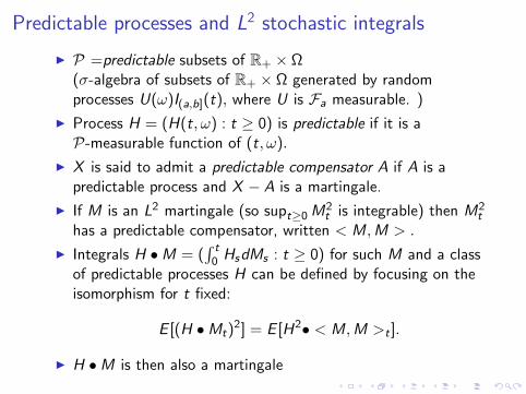
Predictable processes and L2 stochastic integrals

I P =predictable subsets of R+ × Ω(σ-algebra of subsets of R+ × Ω generated by randomprocesses U(ω)I(a,b](t), where U is Fa measurable. )

I Process H = (H(t, ω) : t ≥ 0) is predictable if it is aP-measurable function of (t, ω).

I X is said to admit a predictable compensator A if A is apredictable process and X − A is a martingale.

I If M is an L2 martingale (so supt≥0 M2t is integrable) then M2

t

has a predictable compensator, written < M,M > .

I Integrals H •M = (∫ t0 HsdMs : t ≥ 0) for such M and a class

of predictable processes H can be defined by focusing on theisomorphism for t fixed:

E [(H •Mt)2] = E [H2• < M,M >t ].

I H •M is then also a martingale

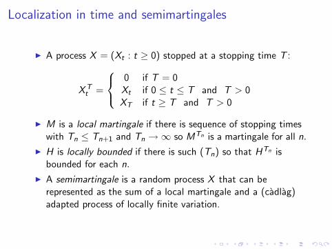
Localization in time and semimartingales

I A process X = (Xt : t ≥ 0) stopped at a stopping time T :

X Tt =

0 if T = 0

Xt if 0 ≤ t ≤ T and T > 0XT if t ≥ T and T > 0

I M is a local martingale if there is sequence of stopping timeswith Tn ≤ Tn+1 and Tn →∞ so MTn is a martingale for all n.

I H is locally bounded if there is such (Tn) so that HTn isbounded for each n.

I A semimartingale is a random process X that can berepresented as the sum of a local martingale and a (cadlag)adapted process of locally finite variation.

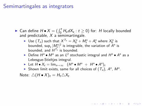
Semimartingales as integrators

I Can define H •X = (∫ t0 HsdXs : t ≥ 0) for: H locally bounded

and predictable, X a semimartingale.I Use (Tn) such that X Tn = X n

0 + Mnt + An

t where X n0 is

bounded, supt |Mnt |2 is integrable, the variation of An is

bounded, and HTn is bounded.I Define Hn •Mn as an L2 stochastic integral and Hn • An as a

Lebesgue-Stieltjes integral.I Let H • Xt = limn→∞ (Hn •Mn + Hn • An)t

I Shown limit exists, same for all choices of (Tn), An, Mn.

Note: 4(H • X )t = Ht4Xt

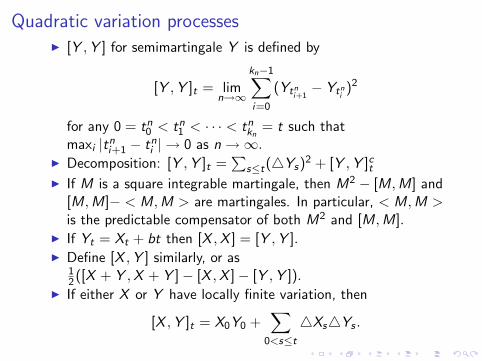
Quadratic variation processesI [Y ,Y ] for semimartingale Y is defined by

[Y ,Y ]t = limn→∞

kn−1∑i=0

(Ytni+1− Ytn

i)2

for any 0 = tn0 < tn

1 < · · · < tnkn

= t such thatmaxi |tn

i+1 − tni | → 0 as n→∞.

I Decomposition: [Y ,Y ]t =∑

s≤t(4Ys)2 + [Y ,Y ]ctI If M is a square integrable martingale, then M2 − [M,M] and

[M,M]− < M,M > are martingales. In particular, < M,M >is the predictable compensator of both M2 and [M,M].

I If Yt = Xt + bt then [X ,X ] = [Y ,Y ].I Define [X ,Y ] similarly, or as

12([X + Y ,X + Y ]− [X ,X ]− [Y ,Y ]).

I If either X or Y have locally finite variation, then

[X ,Y ]t = X0Y0 +∑

0<s≤t

4Xs4Ys .

Example: Brownian motion

Let W denote standard Brownian motion. Then, as well known,[W ,W ]t = [W ,W ]ct =< W ,W >t= t.

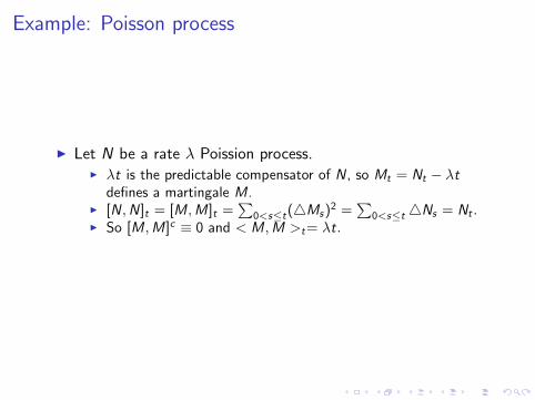
Example: Poisson process

I Let N be a rate λ Poission process.I λt is the predictable compensator of N, so Mt = Nt − λt

defines a martingale M.I [N,N]t = [M,M]t =

∑0<s≤t(4Ms)2 =

∑0<s≤t4Ns = Nt .

I So [M,M]c ≡ 0 and < M,M >t= λt.

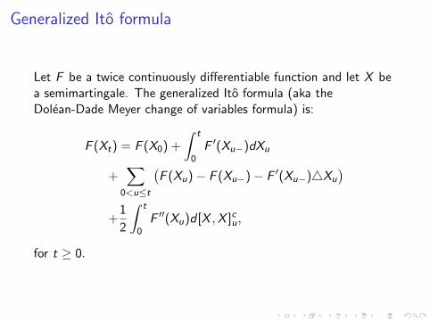
Generalized Ito formula

Let F be a twice continuously differentiable function and let X bea semimartingale. The generalized Ito formula (aka theDolean-Dade Meyer change of variables formula) is:

F (Xt) = F (X0) +

∫ t

0F ′(Xu−)dXu

+∑

0<u≤t

(F (Xu)− F (Xu−)− F ′(Xu−)4Xu

)+

1

2

∫ t

0F ′′(Xu)d [X ,X ]cu,

for t ≥ 0.

PART II: Kingman’s moment bound indiscrete and continuous time

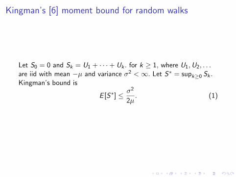
Kingman’s [6] moment bound for random walks

Let S0 = 0 and Sk = U1 + · · ·+ Uk . for k ≥ 1, where U1,U2, . . .are iid with mean −µ and variance σ2 <∞. Let S∗ = supk≥0 Sk .Kingman’s bound is

E [S∗] ≤ σ2

2µ. (1)

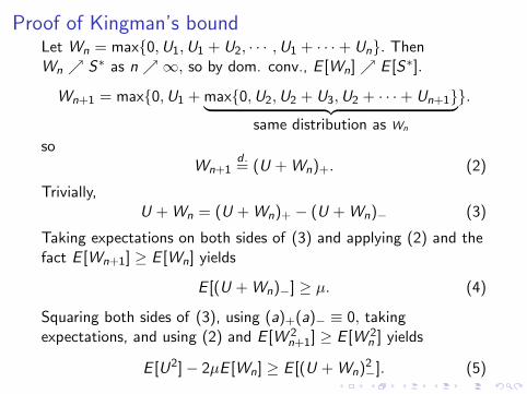
Proof of Kingman’s boundLet Wn = max0,U1,U1 + U2, · · · ,U1 + · · ·+ Un. ThenWn S∗ as n∞, so by dom. conv., E [Wn] E [S∗].

Wn+1 = max0,U1 + max0,U2,U2 + U3,U2 + · · ·+ Un+1︸ ︷︷ ︸same distribution as Wn

.

soWn+1

d .= (U + Wn)+. (2)

Trivially,U + Wn = (U + Wn)+ − (U + Wn)− (3)

Taking expectations on both sides of (3) and applying (2) and thefact E [Wn+1] ≥ E [Wn] yields

E [(U + Wn)−] ≥ µ. (4)

Squaring both sides of (3), using (a)+(a)− ≡ 0, takingexpectations, and using (2) and E [W 2

n+1] ≥ E [W 2n ] yields

E [U2]− 2µE [Wn] ≥ E [(U + Wn)2−]. (5)

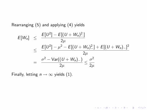
Rearranging (5) and applying (4) yields

E [Wn] ≤E [U2]− E [(U + Wn)2

−]

2µ

≤E [U2]− µ2 − E [(U + Wn)2

−] + E [(U + Wn)−]2

2µ

=σ2 − Var((U + Wn)−)

2µ≤ σ2

2µ

Finally, letting n→∞ yields (1).

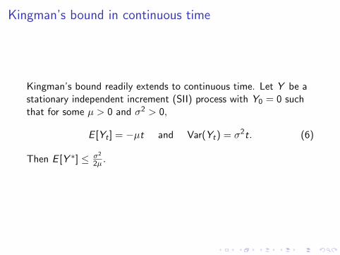
Kingman’s bound in continuous time

Kingman’s bound readily extends to continuous time. Let Y be astationary independent increment (SII) process with Y0 = 0 suchthat for some µ > 0 and σ2 > 0,

E [Yt ] = −µt and Var(Yt) = σ2t. (6)

Then E [Y ∗] ≤ σ2

2µ .

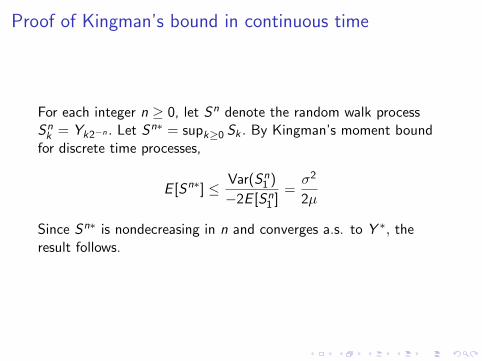
Proof of Kingman’s bound in continuous time

For each integer n ≥ 0, let Sn denote the random walk processSn

k = Yk2−n . Let Sn∗ = supk≥0 Sk . By Kingman’s moment boundfor discrete time processes,

E [Sn∗] ≤ Var(Sn1 )

−2E [Sn1 ]

=σ2

2µ

Since Sn∗ is nondecreasing in n and converges a.s. to Y ∗, theresult follows.

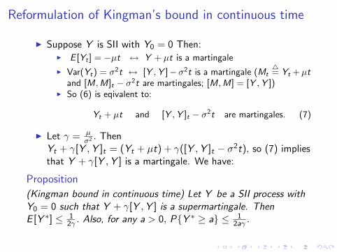
Reformulation of Kingman’s bound in continuous time

I Suppose Y is SII with Y0 = 0 Then:I E [Yt ] = −µt ↔ Y + µt is a martingale

I Var(Yt) = σ2t ↔ [Y ,Y ]−σ2t is a martingale (Mt4= Yt +µt

and [M,M]t − σ2t are martingales; [M,M] = [Y ,Y ])I So (6) is eqivalent to:

Yt + µt and [Y ,Y ]t − σ2t are martingales. (7)

I Let γ = µσ2 . Then

Yt + γ[Y ,Y ]t = (Yt + µt) + γ([Y ,Y ]t − σ2t), so (7) impliesthat Y + γ[Y ,Y ] is a martingale. We have:

Proposition

(Kingman bound in continuous time) Let Y be a SII process withY0 = 0 such that Y + γ[Y ,Y ] is a supermartingale. ThenE [Y ∗] ≤ 1

2γ . Also, for any a > 0, PY ∗ ≥ a ≤ 12aγ .

Part III: Bound on maximum of asupermartingale (no SII assumption,continuous time)

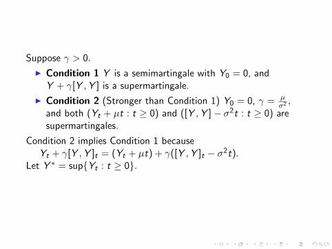
Suppose γ > 0.

I Condition 1 Y is a semimartingale with Y0 = 0, andY + γ[Y ,Y ] is a supermartingale.

I Condition 2 (Stronger than Condition 1) Y0 = 0, γ = µσ2 ,

and both (Yt + µt : t ≥ 0) and ([Y ,Y ]− σ2t : t ≥ 0) aresupermartingales.

Condition 2 implies Condition 1 becauseYt + γ[Y ,Y ]t = (Yt + µt) + γ([Y ,Y ]t − σ2t).

Let Y ∗ = supYt : t ≥ 0.

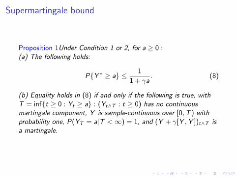
Supermartingale bound

Proposition 1Under Condition 1 or 2, for a ≥ 0 :(a) The following holds:

PY ∗ ≥ a ≤ 1

1 + γa. (8)

(b) Equality holds in (8) if and only if the following is true, withT = inft ≥ 0 : Yt ≥ a : (Yt∧T : t ≥ 0) has no continuousmartingale component, Y is sample-continuous over [0,T ) withprobability one, P(YT = a|T <∞) = 1, and (Y + γ[Y ,Y ])t∧T isa martingale.

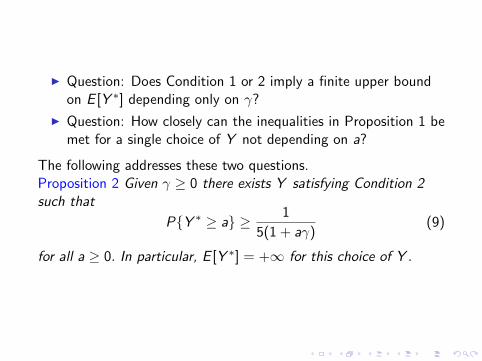
I Question: Does Condition 1 or 2 imply a finite upper boundon E [Y ∗] depending only on γ?

I Question: How closely can the inequalities in Proposition 1 bemet for a single choice of Y not depending on a?

The following addresses these two questions.Proposition 2 Given γ ≥ 0 there exists Y satisfying Condition 2such that

PY ∗ ≥ a ≥ 1

5(1 + aγ)(9)

for all a ≥ 0. In particular, E [Y ∗] = +∞ for this choice of Y .

Part IV. The big jump construction

This construction shows that the bound on PY ∗ ≥ a is tight,and provides a proof of Proposition 2.

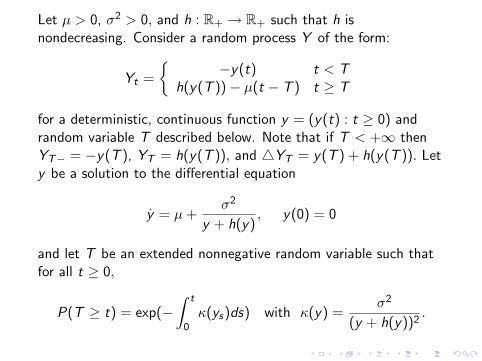
Let µ > 0, σ2 > 0, and h : R+ → R+ such that h isnondecreasing. Consider a random process Y of the form:

Yt =

−y(t) t < T

h(y(T ))− µ(t − T ) t ≥ T

for a deterministic, continuous function y = (y(t) : t ≥ 0) andrandom variable T described below. Note that if T < +∞ thenYT− = −y(T ), YT = h(y(T )), and 4YT = y(T ) + h(y(T )). Lety be a solution to the differential equation

y = µ+σ2

y + h(y), y(0) = 0

and let T be an extended nonnegative random variable such thatfor all t ≥ 0,

P(T ≥ t) = exp(−∫ t

0κ(ys)ds) with κ(y) =

σ2

(y + h(y))2.

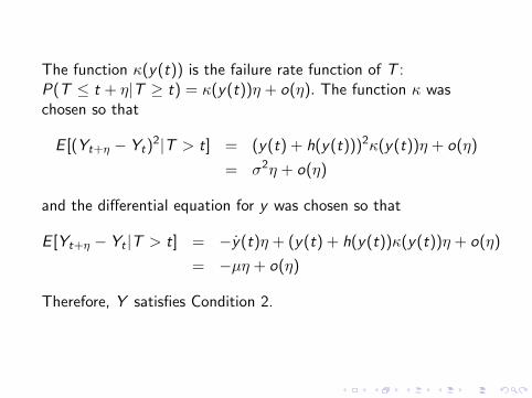
The function κ(y(t)) is the failure rate function of T :P(T ≤ t + η|T ≥ t) = κ(y(t))η + o(η). The function κ waschosen so that

E [(Yt+η − Yt)2|T > t] = (y(t) + h(y(t)))2κ(y(t))η + o(η)

= σ2η + o(η)

and the differential equation for y was chosen so that

E [Yt+η − Yt |T > t] = −y(t)η + (y(t) + h(y(t))κ(y(t))η + o(η)

= −µη + o(η)

Therefore, Y satisfies Condition 2.

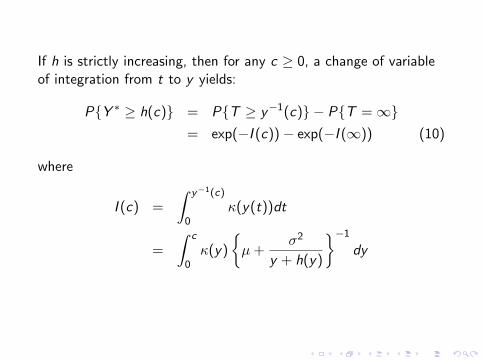
If h is strictly increasing, then for any c ≥ 0, a change of variableof integration from t to y yields:

PY ∗ ≥ h(c) = PT ≥ y−1(c) − PT =∞= exp(−I (c))− exp(−I (∞)) (10)

where

I (c) =

∫ y−1(c)

0κ(y(t))dt

=

∫ c

0κ(y)

µ+

σ2

y + h(y)

−1

dy

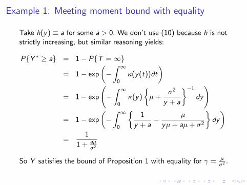
Example 1: Meeting moment bound with equality

Take h(y) ≡ a for some a > 0. We don’t use (10) because h is notstrictly increasing, but similar reasoning yields:

PY ∗ ≥ a = 1− PT =∞

= 1− exp

(−∫ ∞

0κ(y(t))dt

)= 1− exp

(−∫ ∞

0κ(y)

µ+

σ2

y + a

−1

dy

)

= 1− exp

(−∫ ∞

0

1

y + a− µ

yµ+ aµ+ σ2

dy

)=

1

1 + aµσ2

So Y satisfies the bound of Proposition 1 with equality for γ = µσ2 .

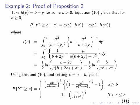
Example 2: Proof of Proposition 2Take h(y) = b + y for some b > 0. Equation (10) yields that forb ≥ 0,

PY ∗ ≥ b + c = exp(−I (c))− exp(−I (∞))

where

I (c) =

∫ c

0

σ2

(b + 2y)2

µ+

σ2

b + 2y

−1

dy

=

∫ c

0

1

b + 2y− µ

µ(b + 2y) + σ2

dy

=1

2ln

(b + 2c

µ(b + 2c) + σ2

)− 1

2ln

(b

µb + σ2

)Using this and (10), and setting c = a− b, yields

PY ∗ ≥ a =

(

µbµb+σ2

) 12

(1 + σ2

µ(2a−b)

) 12 − 1

a ≥ b

1−(

µbµb+σ2

) 12

0 < a ≤ b

(11)

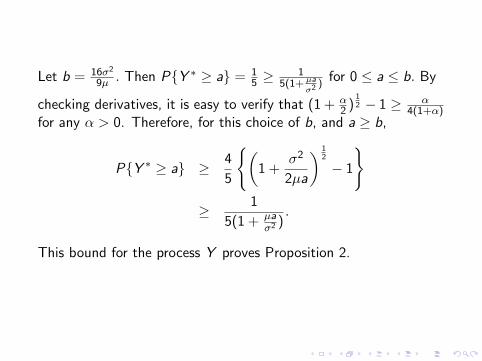
Let b = 16σ2

9µ . Then PY ∗ ≥ a = 15 ≥

15(1+ µa

σ2 )for 0 ≤ a ≤ b. By

checking derivatives, it is easy to verify that (1 + α2 )

12 − 1 ≥ α

4(1+α)for any α > 0. Therefore, for this choice of b, and a ≥ b,

PY ∗ ≥ a ≥ 4

5

(1 +

σ2

2µa

) 12

− 1

≥ 1

5(1 + µaσ2 )

.

This bound for the process Y proves Proposition 2.

Part V. Proof of the upper bound

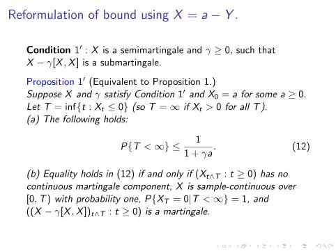
Reformulation of bound using X = a − Y .

Condition 1′ : X is a semimartingale and γ ≥ 0, such thatX − γ[X ,X ] is a submartingale.

Proposition 1′ (Equivalent to Proposition 1.)Suppose X and γ satisfy Condition 1′ and X0 = a for some a ≥ 0.Let T = inft : Xt ≤ 0 (so T =∞ if Xt > 0 for all T ).(a) The following holds:

PT <∞ ≤ 1

1 + γa. (12)

(b) Equality holds in (12) if and only if (Xt∧T : t ≥ 0) has nocontinuous martingale component, X is sample-continuous over[0,T ) with probability one, PXT = 0|T <∞ = 1, and((X − γ[X ,X ])t∧T : t ≥ 0) is a martingale.

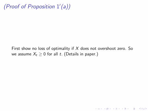
(Proof of Proposition 1′(a))

First show no loss of optimality if X does not overshoot zero. Sowe assume Xt ≥ 0 for all t. (Details in paper.)

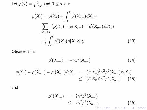
Let p(x) = 11+γa and 0 ≤ s < t.

p(Xt) = p(Xs) +

∫ t

sp′(Xu−)dXu+∑

s<u≤t

(p(Xu)− p(Xu−)− p′(Xu−)4Xu

)+

1

2

∫ t

sp′′(Xu)d [X ,X ]cu (13)

Observe that

p′(Xu−) = −γp2(Xu−) (14)

p(Xu)− p(Xu−)− p′(Xu−)4Xu = (4Xu)2γ2p2(Xu−)p(Xu)

≤ (4Xu)2γ2p2(Xu−) (15)

and

p′′(Xu−) = 2γ2p3(Xu−)

≤ 2γ2p2(Xu−). (16)

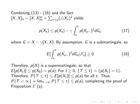
Combining (13) - (16) and the fact[X ,X ]u = [X ,X ]cu +

∑v≤u(4Xv )2 yields

p(Xt) ≤ p(Xs)− γ∫ t

sp(Xu−)2dGu (17)

where G = X − γ[X ,X ]. By assumption, G is a submartingale, so

E [

∫ t

sp(Xu−)2dGu|Fs ] ≥ 0 (18)

Therefore, p(X ) is a supermartingale, so thatE [p(Xt)] ≤ p(X0) = p(a). For t ≥ 0, T ≤ t = p(Xt) = 1.Therefore, PT ≤ t ≤ E [p(Xt)] ≤ p(a) for all t. Thus,PT <∞ = limt→∞ PT ≤ t ≤ p(a), completing the proof ofProposition 1′ (a).

(Proof of Proposition 1′ (b))

To prove the uniqueness of the process constructed to meet thebound, we simply look over last three slides to see when thevarious inequalities used in the upper bound are tight. Details arein the paper.

Part VI. Discrete-time, version I

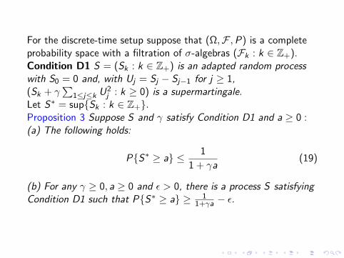
For the discrete-time setup suppose that (Ω,F ,P) is a completeprobability space with a filtration of σ-algebras (Fk : k ∈ Z+).Condition D1 S = (Sk : k ∈ Z+) is an adapted random processwith S0 = 0 and, with Uj = Sj − Sj−1 for j ≥ 1,(Sk + γ

∑1≤j≤k U2

j : k ≥ 0) is a supermartingale.Let S∗ = supSk : k ∈ Z+.Proposition 3 Suppose S and γ satisfy Condition D1 and a ≥ 0 :(a) The following holds:

PS∗ ≥ a ≤ 1

1 + γa(19)

(b) For any γ ≥ 0, a ≥ 0 and ε > 0, there is a process S satisfyingCondition D1 such that PS∗ ≥ a ≥ 1

1+γa − ε.

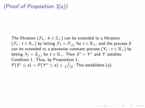
(Proof of Proposition 3(a))

The filtration (Fk : k ∈ Z+) can be extended to a filtration(Ft : t ∈ R+) by letting Ft = Fbtc for t ∈ R+, and the process Scan be extended to a piecewise constant process (Yt : t ∈ R+) byletting Yt = Sbtc for t ∈ R+. Then S∗ = Y ∗ and Y satisfiesCondition 1. Thus, by Proposition 1,PS∗ ≤ a = PY ∗ ≤ a ≤ 1

1+γa . This establishes (a).

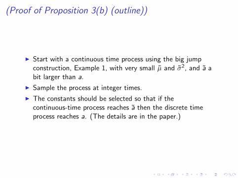
(Proof of Proposition 3(b) (outline))

I Start with a continuous time process using the big jumpconstruction, Example 1, with very small µ and σ2, and a abit larger than a.

I Sample the process at integer times.

I The constants should be selected so that if thecontinuous-time process reaches a then the discrete timeprocess reaches a. (The details are in the paper.)

Part VII. Discrete-time, version II

Conditions 1 and 2 yield the same bounds for continuous time. Thesame is not true in discrete time. In this section we explore thediscrete time version of Condition 2, which we call Condition D2.

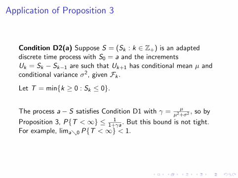
Application of Proposition 3

Condition D2(a) Suppose S = (Sk : k ∈ Z+) is an adapteddiscrete time process with S0 = a and the incrementsUk = Sk − Sk−1 are such that Uk+1 has conditional mean µ andconditional variance σ2, given Fk .

Let T = mink ≥ 0 : Sk ≤ 0.

The process a− S satisfies Condition D1 with γ = µµ2+σ2 , so by

Proposition 3, PT <∞ ≤ 11+γa . But this bound is not tight.

For example, lima0 PT <∞ < 1.

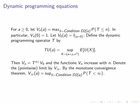
Dynamic programming equations

For a ≥ 0, let Vn(a) = maxS∼Condition D2(a) PT ≤ n. In

particular, Vn(0) = 1. Let V0(a) = Ia=0. Define the dynamicprogramming operator T by

TU(a) = supX∼(a+µ,σ2)

E [U(X )].

Then Vn = T nV0 and the functions Vn increase with n. Denotethe (pointwise) limit by V∞. By the monotone convergencetheorem, V∞(a) = supS∼Condition D2(a) PT <∞.

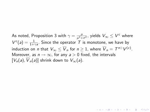
As noted, Proposition 3 with γ = µµ2+σ2 , yields V∞ ≤ V c where

V c(a) = 11+γa . Since the operator T is monotone, we have by

induction on n that V∞ ≤ V n for n ≥ 1, where V n = T nV (c).Moreover, as n→∞, for any a > 0 fixed, the intervals[Vn(a),V n(a)] shrink down to V∞(a).

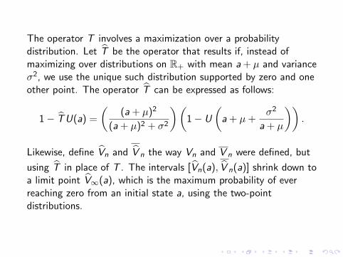
The operator T involves a maximization over a probabilitydistribution. Let T be the operator that results if, instead ofmaximizing over distributions on R+ with mean a + µ and varianceσ2, we use the unique such distribution supported by zero and oneother point. The operator T can be expressed as follows:

1− T U(a) =

((a + µ)2

(a + µ)2 + σ2

)(1− U

(a + µ+

σ2

a + µ

)).

Likewise, define Vn and V n the way Vn and V n were defined, but

using T in place of T . The intervals [Vn(a), V n(a)] shrink down toa limit point V∞(a), which is the maximum probability of everreaching zero from an initial state a, using the two-pointdistributions.

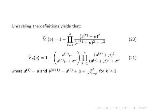
Unraveling the definitions yields that:

Vn(a) = 1−n∏

k=1

(a(k) + µ)2

(a(k) + µ)2 + σ2(20)

V n(a) = 1−

(a(n)µ

a(n)µ+ σ2

)n∏

k=1

(a(k) + µ)2

(a(k) + µ)2 + σ2(21)

where a(1) = a and a(k+1) = a(k) + µ+ σ2

a(k)+µfor k ≥ 1.

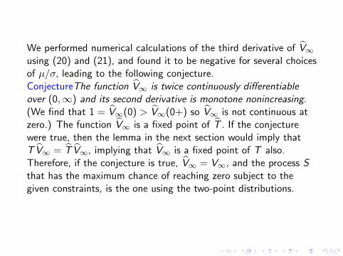
We performed numerical calculations of the third derivative of V∞using (20) and (21), and found it to be negative for several choicesof µ/σ, leading to the following conjecture.ConjectureThe function V∞ is twice continuously differentiableover (0,∞) and its second derivative is monotone nonincreasing.(We find that 1 = V∞(0) > V∞(0+) so V∞ is not continuous atzero.) The function V∞ is a fixed point of T . If the conjecturewere true, then the lemma in the next section would imply thatT V∞ = T V∞, implying that V∞ is a fixed point of T also.Therefore, if the conjecture is true, V∞ = V∞, and the process Sthat has the maximum chance of reaching zero subject to thegiven constraints, is the one using the two-point distributions.

Part VIII. A lemma providing insight

Let m > 0 and σ2 ≥ 0. Let X have the unique probabilitydistribution with mean m and variance σ2 supported by 0, b or

b for some point b > 0. Specifically, b = m2+σ2

m ,

PX = b =m2

m2 + σ2, and PX = 0 =

σ2

m2 + σ2.

LemmaSuppose φ : R+ → [0, 1] is a continuous function which is twicecontinuously differentiable over (0,∞). Suppose φ′′ isnonincreasing. (It easily follows that φ is nonincreasing and convex.For example, φ(x) = 1

1+x .) Let X be any nonnegative random

variable with mean m and variance σ2. Then E [φ(X )] ≤ E [φ(X )].

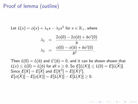
Proof of lemma (outline)

Let L(x) = φ(x) + λ1x − λ2x2 for x ∈ R+, where

λ1 =2φ(0)− 2φ(b) + bφ′(0)

b

λ2 =φ(0)− φ(b) + bφ′(0)

b2.

Then L(0) = L(b) and L′(b) = 0, and it can be shown shown thatL(x) ≤ L(0) = L(b) for all x ≥ 0. So E [L(X )] ≤ L(0) = E [L(X )].Since E [X ] = E [X ] and E [X 2] = E [(X )2],E [φ(X )]− E [φ(X )] = E [L(X )]− E [L(X )] ≥ 0.

Part IX. Comparison to Doob’s moment bounds

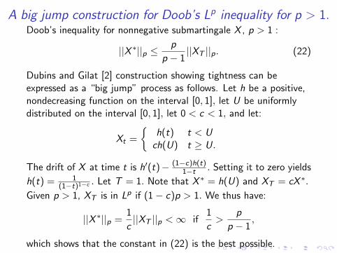
A big jump construction for Doob’s Lp inequality for p > 1.Doob’s inequality for nonnegative submartingale X , p > 1 :

||X ∗||p ≤p

p − 1||XT ||p. (22)

Dubins and Gilat [2] construction showing tightness can beexpressed as a “big jump” process as follows. Let h be a positive,nondecreasing function on the interval [0, 1], let U be uniformlydistributed on the interval [0, 1], let 0 < c < 1, and let:

Xt =

h(t) t < U

ch(U) t ≥ U.

The drift of X at time t is h′(t)− (1−c)h(t)1−t . Setting it to zero yields

h(t) = 1(1−t)1−c . Let T = 1. Note that X ∗ = h(U) and XT = cX ∗.

Given p > 1, XT is in Lp if (1− c)p > 1. We thus have:

||X ∗||p =1

c||XT ||p <∞ if

1

c>

p

p − 1,

which shows that the constant in (22) is the best possible.

The analysis of [2] is related to work of Blackwell and Dubins [1],which makes a connection to the Hardy-Littlewood maximalfunction [3], h, of a nondecreasing integrable function g on [0, 1],defined as follows:

h(t) =1

1− t

∫ 1

tg(u)du.

In fact, h is the unique function such that a process that follows hup until time U, and then jumps and sticks to value g(U), is amartingale.

References I

D. Blackwell and L.E. Dubins.A converse to the dominated convergence theorem.Ill. J. Math., 7:508–514, 1963.

L. E. Dubins and David Gilat.On the distribution of maxima of martingales.Proc. Amer. Math. Soc., 68(3):337–338, 1978.

G. H. Hardy and J. E. Littlewood.A maximal theorem with function-theoretic applications.Acta Math., 54(1):81–116, 1930.

J. Jacod.Calcul stochastique et problemes de martingales, LectureNotes in Math., vol. 714.Springer-Verlag, New York, 1979.

References II

O. Kallenberg.Foundations of Modern Probability (2nd ed.).Springer, 2002.

J.F.C. Kingman.Some inequalities for the queue GI/G/1.Biometrika, 49(3/4):315–324, December 1962.

P.A. Meyer.Un cours sur les integrales stochastiques, pages 246–400.Springer-Verlag, New York, 1976.

P. Protter.Stochastic Integration and Differential Equations (2nd ed.).Springer, 2004.

E. Wong and B. Hajek.Stochastic processes in engineering systems.Springer-Verlag, New York, 1985.

References III