Embed Size (px)
Citation preview

A discrete space and time before the big bang
Martin Bojowald
The Pennsylvania State University
Institute for Gravitation and the Cosmos
University Park, PA
Time before the big bang – p.1

Gravity
The gravitational field is the only known fundamental force notyet quantized completely, despite of more than six decades ofresearch. Difficulties arise due to two key properties:
Time before the big bang – p.2

Gravity
The gravitational field is the only known fundamental force notyet quantized completely, despite of more than six decades ofresearch. Difficulties arise due to two key properties:
→ Although it is weak in usual regimes of particle physics, itbecomes the dominant player on cosmic scales. Strongquantum gravity effects must appear in large gravitational fields:very early universe and black holes. Then, the classical fieldgrows without bound, implying space-time singularities.
→ Equivalence principle: gravity isa manifestation of space-time ge-ometry. The full space-time met-ric gµν is thus the physical objectto be quantized non-perturbatively,rather than using perturbations hµνon a background space-time ηµν .
Time before the big bang – p.2

Canonical quantum gravity
Combine general relativity and quantum mechanics:“Substitutions” (q, p) −→ (qab, p
ab) where qab is the spatial metricappearing in the line element
ds2 = −N2dt2 + qab(dxa +Nadt)(dxb +N bdt)
for a dynamical, curved space-time, and pab its momentumrelated geometrically to extrinsic curvatureKab = 1
2N (Ltqab − 2D(aNb)).
Time before the big bang – p.3
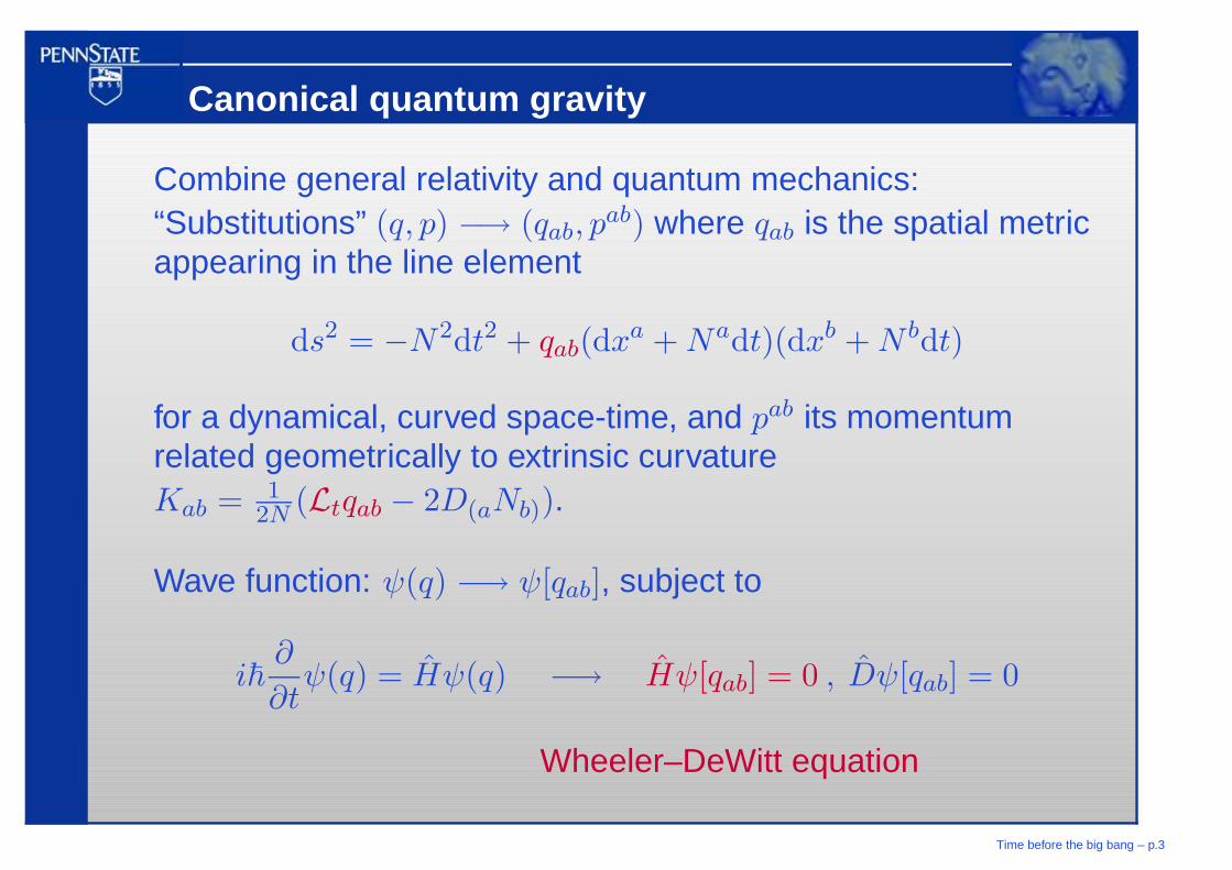
Canonical quantum gravity
Combine general relativity and quantum mechanics:“Substitutions” (q, p) −→ (qab, p
ab) where qab is the spatial metricappearing in the line element
ds2 = −N2dt2 + qab(dxa +Nadt)(dxb +N bdt)
for a dynamical, curved space-time, and pab its momentumrelated geometrically to extrinsic curvatureKab = 1
2N (Ltqab − 2D(aNb)).
Wave function: ψ(q) −→ ψ[qab], subject to
i~∂
∂tψ(q) = Hψ(q) −→ Hψ[qab] = 0 , Dψ[qab] = 0
Wheeler–DeWitt equation
Time before the big bang – p.3

Space-time structure
Difficulty: tensor fields such as qab subject to transformationlaws, but theory must be coordinate invariant. In generallycovariant systems, non-linear change of coordinates
qab 7→∂x′a
′
∂xa∂x′b
′
∂xbqa′b′
would lead to coordinate dependent factors not represented onHilbert space.
Moreover, manifold itself is part of the solution in generalrelativity, not known before quantum operators are defined.
Time before the big bang – p.4

Space-time structure
Difficulty: tensor fields such as qab subject to transformationlaws, but theory must be coordinate invariant. In generallycovariant systems, non-linear change of coordinates
qab 7→∂x′a
′
∂xa∂x′b
′
∂xbqa′b′
would lead to coordinate dependent factors not represented onHilbert space.
Moreover, manifold itself is part of the solution in generalrelativity, not known before quantum operators are defined.
Guides search for suitable building blocks of quantum gravity.One solution: Use index-free objects, holonomies/fluxes.
Consequence: Configuration space given by holonomies iscompact, geometrical fluxes become derivative operators oncompact space with discrete spectra: discrete space.
Time before the big bang – p.4

Loop quantum gravity
Scalar objects based on new variables: canonical transformation
(qab, pab) 7→ (−ǫijkebj(∂[ae
kb] +
12eckela∂[ce
lb]) + ebiKab, |det(ejb)|eai )
using co-triad eia (three co-vector fields) such that eiaeib = qab.
and its inverse eai .
More compactly: (qab, pcd) 7→ (Aia, E
bj ) with Ashtekar connection
Aia and densitized triad Ebj . Gauge group SO(3) for rotations.
Time before the big bang – p.5

Loop quantum gravity
Scalar objects based on new variables: canonical transformation
(qab, pab) 7→ (−ǫijkebj(∂[ae
kb] +
12eckela∂[ce
lb]) + ebiKab, |det(ejb)|eai )
using co-triad eia (three co-vector fields) such that eiaeib = qab.
and its inverse eai .
More compactly: (qab, pcd) 7→ (Aia, E
bj ) with Ashtekar connection
Aia and densitized triad Ebj . Gauge group SO(3) for rotations.
Variables as in non-Abelian gauge theories: use “lattice”formulation.For any curve e and surface S in space, define holonomies andfluxes
he(A) = P exp
∫
eAiaτie
adt , FS(E) =
∫
Sd2ynaE
ai τi
with tangent vector ea, co-normal na and Pauli matrices τi.Time before the big bang – p.5

Representation
Holonomies give connection, can be used as non-tensorialconfiguration variables: wave functions ψ[he(A
ia)].
Take values in SU(2): compact.
[Quantization on compact space, e.g. circle: wave functions ψn(φ) = exp(inφ) with
integer n. Momentum eigenvalues discrete: pψn(φ) = −i~dψn(φ)/dφ = ~nψn(φ).]
Fluxes canonically conjugate, become derivative operators onSU(2), analogous to angular momentum: discrete spectra.
Time before the big bang – p.6

Representation
Holonomies give connection, can be used as non-tensorialconfiguration variables: wave functions ψ[he(A
ia)].
Take values in SU(2): compact.
[Quantization on compact space, e.g. circle: wave functions ψn(φ) = exp(inφ) with
integer n. Momentum eigenvalues discrete: pψn(φ) = −i~dψn(φ)/dφ = ~nψn(φ).]
Fluxes canonically conjugate, become derivative operators onSU(2), analogous to angular momentum: discrete spectra.
Construction: spatial metric qab −→ densitized triad Eai −→ fluxoperator. Thus, spatial geometry is discrete.
−→ Volumes of point sets can only increase in discrete stepswhen they are enlarged.−→ Dynamical growth such as universe expansion appears indiscrete steps.
Time before the big bang – p.6

Scale of discreteness
Dimensional argument: Planck length ℓP =√G~ ≈ 10−35m.
[Analogy in quantum mechanics: Bohr radius ∝ ~2/mee2]
Precise role of Planck length to be determined from calculations.
Loop quantum gravity:√γℓP with γ ≈ 0.238
(from black hole entropy).Discreteness levels of geometry:
√γℓPn with integer n.
Time before the big bang – p.7

Scale of discreteness
Dimensional argument: Planck length ℓP =√G~ ≈ 10−35m.
[Analogy in quantum mechanics: Bohr radius ∝ ~2/mee2]
Precise role of Planck length to be determined from calculations.
Loop quantum gravity:√γℓP with γ ≈ 0.238
(from black hole entropy).Discreteness levels of geometry:
√γℓPn with integer n.
Typical interplay for quantum gravity:−→ state more semiclassical for higher excitations, larger n−→ higher n implies coarser discreteness
Quantum behavior at small n and discreteness at large n givesdeviations from classical theory.
Leverage to be exploited by observations, despite smallness ofℓP.
Time before the big bang – p.7

Quantum cosmology
Discreteness has dynamical implications, most easily seen forisotropic spaces: |E| = a2/4 (scale factor a), A = a/2.
Orthonormal states 〈A|µ〉 = eiµA/2, µ ∈ R and basic operators
eiµ′A/2|µ〉 = |µ+µ′〉E|µ〉 = 1
6γℓ2Pµ|µ〉
from E = −13 i~γG
∂∂A .
Time before the big bang – p.8

Quantum cosmology
Discreteness has dynamical implications, most easily seen forisotropic spaces: |E| = a2/4 (scale factor a), A = a/2.
Orthonormal states 〈A|µ〉 = eiµA/2, µ ∈ R and basic operators
eiµ′A/2|µ〉 = |µ+µ′〉E|µ〉 = 1
6γℓ2Pµ|µ〉
from E = −13 i~γG
∂∂A .
Operators follow from full holonomy-flux operators.Representation inequivalent to Wheeler–DeWitt representation:
eiµ′A/2 not continuous in µ′; E with discrete spectrum.
Time before the big bang – p.8
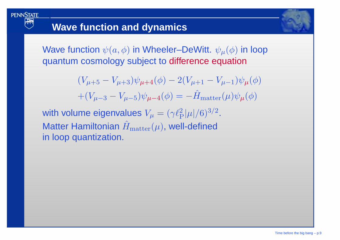
Wave function and dynamics
Wave function ψ(a, φ) in Wheeler–DeWitt. ψµ(φ) in loopquantum cosmology subject to difference equation
(Vµ+5 − Vµ+3)ψµ+4(φ) − 2(Vµ+1 − Vµ−1)ψµ(φ)
+(Vµ−3 − Vµ−5)ψµ−4(φ) = −Hmatter(µ)ψµ(φ)
with volume eigenvalues Vµ = (γℓ2P|µ|/6)3/2.
Matter Hamiltonian Hmatter(µ), well-definedin loop quantization.
Time before the big bang – p.9

Wave function and dynamics
Wave function ψ(a, φ) in Wheeler–DeWitt. ψµ(φ) in loopquantum cosmology subject to difference equation
(Vµ+5 − Vµ+3)ψµ+4(φ) − 2(Vµ+1 − Vµ−1)ψµ(φ)
+(Vµ−3 − Vµ−5)ψµ−4(φ) = −Hmatter(µ)ψµ(φ)
with volume eigenvalues Vµ = (γℓ2P|µ|/6)3/2.
Matter Hamiltonian Hmatter(µ), well-definedin loop quantization.
µ with both signs: evolution continues to new branchpreceding big bang (at µ = 0), provided automatically.
Sign sgn(µ) from handedness of triad, spatial orientation.Implied by search for quantizable index-free objects.Orientation flips while going through classical singularity,universe “turns inside out”.
Time before the big bang – p.9

Role of spatial discreteness
Absence of a singularity: Difference equation uniquely connectswave function at both sides of vanishing volume µ = 0.
discretespace
−→
•discrete steps ofwave function evolution
•no diverging a−3
in matter Hamiltonian
−→ time beforethe big bang
Time before the big bang – p.10

Role of spatial discreteness
Absence of a singularity: Difference equation uniquely connectswave function at both sides of vanishing volume µ = 0.
discretespace
−→
•discrete steps ofwave function evolution
•no diverging a−3
in matter Hamiltonian
−→ time beforethe big bang
Inverse in matter Hamiltoniane.g. Hφ = 1
2a−3p2
φ + a3V (φ) forscalar φ with momentum pφ.
a−3 bounded operator whenexpressed through holonomiesand fluxes.
0
2
4
6
8
10
12
0 0.1 0.2 0.3 0.4 0.5 0.6 0.7 0.8
a
l=0l=1/4l=1/2l=3/4
l=0.999
Time before the big bang – p.10

The role of matter
Absence of singularity independent of form of matter:recurrence of difference equation
(Vµ+5 − Vµ+3)ψµ+4(φ) − 2(Vµ+1 − Vµ−1)ψµ(φ)
+(Vµ−3 − Vµ−5)ψµ−4(φ) = −Hmatter(µ)ψµ(φ)
not affected.
Time before the big bang – p.11

The role of matter
Absence of singularity independent of form of matter:recurrence of difference equation
(Vµ+5 − Vµ+3)ψµ+4(φ) − 2(Vµ+1 − Vµ−1)ψµ(φ)
+(Vµ−3 − Vµ−5)ψµ−4(φ) = −Hmatter(µ)ψµ(φ)
not affected.
But: Orientation reversal key in transition through singularity.
Parity violation on matter side (Hmatter(µ) 6= Hmatter(−µ)) makesequation non-invariant under µ 7→ −µ.
State of the universe before and after the big bang must then bedifferent. Important to understand origin of the universe beforethe big bang.
Time before the big bang – p.11

Effective picture
Difficult to analyze more generally, but effective equationsavailable:Solve dynamics for expectation value 〈V 〉 of volume directly,rather than using wave function with its interpretationalproblems. Scheme:
d
dt〈V 〉 =
〈[V , H ]〉i~
= · · ·
in terms of other degrees of freedom such as 〈 exp(iA)〉 but alsohigher moments of the state, in particular fluctuations.
Time before the big bang – p.12

Effective picture
Difficult to analyze more generally, but effective equationsavailable:Solve dynamics for expectation value 〈V 〉 of volume directly,rather than using wave function with its interpretationalproblems. Scheme:
d
dt〈V 〉 =
〈[V , H ]〉i~
= · · ·
in terms of other degrees of freedom such as 〈 exp(iA)〉 but alsohigher moments of the state, in particular fluctuations.
Infinitely many coupled equations in general, but closely relatedsolvable model available where [V , H ] is linear in basicoperators.Isotropic model with free, massless scalar: plays the role of theharmonic oscillator for cosmology.
Time before the big bang – p.12

Conclusions
Loop quantum gravity establishes discrete fundamental pictureof space based on well-defined canonical quantization of gravity.
Space-time dynamics can be analyzed in cosmological models.Direct route from discrete space to non-singular evolution:time before the big bang.
Time before the big bang – p.13

Conclusions
Loop quantum gravity establishes discrete fundamental pictureof space based on well-defined canonical quantization of gravity.
Space-time dynamics can be analyzed in cosmological models.Direct route from discrete space to non-singular evolution:time before the big bang.
Absence of singularity independent of precise form of matter,but details play a role for the precise transition. In particular,orientation reversal at the place of the classical singularity.Thus, parity violating matter affects how pre- and post-big bangphysics connect.
Yet to be put into equations (torsion coupling), but effectiveequations allow more straightforward analysis. Show possibilityof parity asymmetric solutions even from gravity itself: statespreads during evolution, fluctuations in general not symmetric.
Time before the big bang – p.13