Marriage Market Effects of a Wealth Shock in Bangladesh

A. Mushfiq Mobarak

Department of Economics and Institute of Behavioral Science Randall Kuhn

Institute of Behavioral Science Christina Peters

Department of Economics

University of Colorado at Boulder

Abstract Research has documented that conditions of marriage for women in South Asia such as dowries, consanguinity, early marriage, or spousal age gaps are important influences on her children’s and her own subsequent life outcomes. However, research on the determinants of these conditions of marriage has remained relatively sparse and largely descriptive. Since a variety of determinants can co-vary with each other and with unobservable characteristics, drawing causal inferences has been difficult. This paper uses the construction of a flood protection embankment in Matlab district in rural Bangladesh coupled with data on the universe of all 52,000 marriage decisions in that district between 1982 and 1996 to examine whether marital prospects for protected households improved after embankment construction relative to unprotected households living on the other side of the river. A variety of evidence is supportive that the embankment led to exogenous quasi-experimental variation in risk exposure and endowments across groups of households. Consistent with two-sided matching models of the marriage market, we show that protected households commanded larger dowries, and married into families with more land, but that there were only weak effects on age at marriage. The embankment largely benefited farmers, and these marriage market effects are confirmed in a triple difference by occupation. Protected households were less likely to marry into families in different occupations, and to marry biological relatives after embankment construction relative to those that remained unprotected. Estimates based on the subset of families with multiple marriages on either side of the embankment (where we can include household fixed effects) indicate that the same family is 40% less likely to marry a younger child to a biological relative after they are protected by embankment, compared to their older child who married prior to the embankment construction. Marrying consanguineously reduces the need for dowry payments, which seems to be the main mechanism driving this result. JEL Codes: O1, J12, O13 Keywords: Marriage, Embankment, Flood Protection, Consanguinity

January, 2007; Third Draft. Comments Welcome

Correspondence: mobarak@colorado.edu; 303-492-8872. We thank Andrew Foster, Grant Miller, Murat Iyigun, Aloysius Siow, Eric Edmonds, Paul Schultz and seminar participants at the University of Washington at Seattle, the University of British Columbia, Penn State, Yale School of Management, University of Colorado at Boulder (IBS), 9th BREAD Conference, and at the Econometric Society meetings for helpful comments and discussion.

1

1. Introduction

Marriage is one of the most important socio-economic institutions in South Asia,

where brides’ families are reported to spend up to three to four times their assets or six

times their annual incomes on dowries (Suran et al, 2004; Rao, 1993), and about twice

that amount on lavish wedding celebrations in addition (Bloch, Rao and Desai, 2004).

Since a woman often migrates to a new area and almost always becomes a member of a

new family at the time of marriage, her marital prospects have important implications for

her subsequent life outcomes. This paper exploits a unique natural experiment to

examine how an exogenous change in certain households’ socio-economic status and risk

exposure following a flood embankment construction manifests itself in marriage market

outcomes.

Characteristics of the bride’s family at the time of marriage in conjunction with

the characteristics of her spouse and his family determine the conditions of marriage such

as dowries, marrying biological relatives, and age at marriage, which in turn affect

subsequent socio-economic outcomes for the woman and her children (Dalmia, 2004;

Rao, 1993). Several studies conducted in India and Bangladesh report that dowries can

impact the likelihood that the woman will have to endure domestic violence (Jahan, 1991;

Suran et al, 2004; Bloch and Rao, 2002), and early marriage and a larger spousal age gap

lower the woman’s social status in her husband’s home, her school attainment, health

status, and her control over reproductive choices (Tiemoko, 2001; Wickrama and Lorenz,

2002; Jensen and Thornton, 2003; UNICEF 2005; Field and Ambrus, 2005). Marrying a

cousin or uncle can decrease the amount of dowry required (Caldwell et al., 1983; Bittles,

1994), but increases the risk of genetic diseases among offspring (Bittles, 2001).

2

Although the literature on the consequences of marriage is large, the evidence on

the determinants of the conditions of spousal matching is relatively sparse. The evidence

that exists is mostly qualitative or descriptive (e.g. Fruzzetti, 1982; Huq and Amin, 2001)

and typically does not account for multiple determinants of marital prospects that can co-

vary. Rao (1993), Deolalikar and Rao (1998), Dalmia and Lawrence (2001), and Dalmia

(2004) control for multiple covariates in regressions on survey data from rural India and

show that older, taller, more educated grooms of high caste living in areas with a larger

supply of potential brides command larger dowries, and that spouses mate assortatively in

age and education. Since a family can offer compensating differentials along many

dimensions in order to secure a desirable match, and since a spouse from a family with

greater assets, education, or income is likely to differ in unobservable ways from spouses

from poorer families, it becomes difficult to draw causal inferences from this data. Not

all relevant family characteristics are observable in survey data, and the samples used in

the cited studies are cross-sectional and relatively small (141 households in Rao’s papers,

and 905 households in Dalmia’s papers).

Our research design exploits a natural experiment in Bangladesh that caused a

discrete improvement in socio-economic conditions for some families in order to

examine how the marriage market responds to such changes. More specifically, we use

panel data on the entire universe of 33,000 marriages (or 52,000 marriage decisions)

contracted in the 141-village Matlab demographic surveillance area in eastern

Bangladesh between 1982 and 1996 to investigate whether there were differential

changes in the conditions of marriage for the subset of households that were protected

against flood risk by a river embankment following its construction in 1987. A variety of

3

evidence presented in section 2 is supportive of the claim that the embankment led to

exogenous quasi-experimental variation in risk exposure and endowments across groups

of households. We report difference-in-difference regression results on the full sample,

and add household fixed effects for the sub-sample of families that contracted marriages

both before and after embankment construction (e.g. for two different siblings), so that

unobserved differences across households are controlled for.

We first identify the first-order impacts of the embankment construction on basic

socio-economic outcomes through a survey of project documents, by directly

interviewing Matlab residents during fieldwork we conducted in 2005, and using our own

analysis of pre- and post- embankment wealth and mortality data. The major effect of the

embankment was to extend the crop growing season, thereby increasing relative wealth

for households on the protected side, especially among those engaged in farming. The

embankment also changed mortality patterns with the protected now relatively less likely

to die of diarrheal diseases and more likely die in old age of chronic conditions. The

embankment likely had multiple channels of influence on the marriage market behavior

of Matlab households (increased wealth, reduced risk exposure and increased ability to

pay dowry for the protected, and possible indirect impacts on the unprotected through

marriage market competition). We therefore construct some stylized two-sided matching

models of the marriage market in order to generate predictions for different types of

outcomes, and to set up a context within which to interpret our empirical results. A

simple transferable utility model predicts that if the embankment’s primary contribution

is to lower flood risk exposure, then we should observe negative assortative matching in

protection post-embankment. The unprotected have the largest marginal gain from

4

bonding with a protected family, and are therefore willing to pay the most to secure that

match. A corollary is that the protected should receive larger dowries following

embankment construction. A more general model that relaxes the transferable utility

assumption and allows for search frictions delivers the further (numerical) predictions

that (a) greater search frictions for spouses located further away would reduce negative

assortativeness in protection status, and (b) the protected are most likely to secure better

matches along characteristics that are complementary. For example, if the wealth that a

man and woman bring in to a marriage are complementary inputs in generating marital

surplus, then the protected would in general choose to (and be able to) marry into

wealthier households. If age at marriage is not a complementary input, protection will

not necessarily change spousal age or age gaps, since the protected are not willing to pay

relatively more than the unprotected for this characteristic. But if age is a relevant

consideration for spousal choice, its effect will get capitalized into the dowry transfer,

and thus age may bear some relationship to protection status if the embankment changes

the ability to pay dowry.

The empirical results are broadly consistent with the main theoretical predictions,

and in conjunction with the theory, they shed light on some features of the embankment

and the marriage market in Bangladesh. The data show that individuals from protected

households experienced a 3 percent higher likelihood of marrying into households with

above average wealth (as measured by land ownership) post embankment relative to

those that remained unprotected. The embankment had a larger wealth impact on farmers

who benefited most from the extended growing season, and triple difference (pre/post,

un/protected, by occupation) results indicate that agricultural households protected by the

5

embankment had much larger increases in the probability of marrying into wealthier

households (5 percentage point increase for protected farmers compared to 0.3 for non-

farmers). Protected men command larger dowries following embankment construction.

Both protected men and women exhibit a differentially larger ability to postpone

marriage, and protected women are able to marry younger men, but these effects are

statistically and quantitatively weaker. There is no evidence of assortative matching in

protection status in either direction (although there is positive matching by wealth),

which coupled with the observation that people are more likely marry others on the same

side of the river prior to embankment construction, suggests that search frictions are quite

important in this market. This is also consistent with our fieldwork findings that the

direct wealth effect of the embankment was more substantial than its risk mitigation

effects. We do find that unprotected households remain relatively more likely to marry

into different occupations, which suggests that households use the marriage market to

diversify their exposure to risk (Rosenzweig and Stark, 1989).

Our empirical analysis also focuses on the determinants of consanguinity – the

practice of marrying biological relatives – which is surprisingly common in many parts of

Bangladesh, in neighboring India and Pakistan, and more generally in the developing

countries of Asia and Africa.1 However, such marriages impose adverse biological risk

on children in the increased likelihood of receiving two copies of a deleterious gene from

1 A conservative estimate shows that in the mainly Muslim countries of North Africa, West and Central Asia, and in large parts of South Asia, marriage between close relatives account for 20 percent to 50 percent of all unions, with a further 2.8 billion people in countries where 1 percent to 10 percent of marriages are between biological relatives (Bittles et al., 2001; http://www.consang.net). As a specific example, the 1990/1991 Pakistan Demographic and Health Survey revealed that cousin marriages were the social norm, with 50.4 percent of marriages between first cousins and a further 10.4 percent between second cousins, and in one Pakistani group 77.1 percent of marriages were consanguineous (Hashmi, 1997). In the coastal area of south-eastern Bangladesh, about 18 percent of all births accrued to consanguineous households in 1985-86 (Khan, 2001).

6

parents. Child morbidity and mortality rates are shown to be statistically larger among

consanguineous progeny (Bittles and Makov, 1988; Bittles, 2001; Shah et al., 1998).2

Given these observed risks, the question then becomes, what conditions induce a couple

to accept such a marriage type?

In household fixed effects estimates, protected households show a 3.3 percentage

point drop (a 40 percent decrease at the mean) in the likelihood of forming

consanguineous unions following the construction of the embankment relative to

households living on the other side of the river left unprotected. While multiple

mechanisms can link flood protection to consanguinity prevalence, ancillary evidence

indicates that the most likely explanation is that marrying consanguineously reduces the

need for dowry payments which are often difficult for brides from poor families to make,

and this dowry constraint is relaxed for protected households following embankment

construction.3 Since a bride’s parents often do not have either cash on hand or access to

credit to make the up-front dowry payment, they use within-family marriage (where it

becomes possible to promise ex-post payments) as a substitute.

The rest of the paper is organized as follows. In the next two sections, we

describe the setting and our data sources, and present evidence in support of treating the

Meghna-Dhonogoda embankment as a natural experiment that created quasi-random

variation in household exposure to environmental risk. Section 4 describes the direct

2 For instance, in their study of consanguinity in Pakistan, Shah et al. (1998) conclude that when two first-cousins marry, they are 18 percent more likely to experience the death of one of their children before the child is 5 years old. Bittles (2001) reports that child morbidity rates are between 1 percent and 4 percent higher for consanguineous children. Selection issues are generally not adequately address in any of these studies. 3 Other possible explanations for which there is less support in the data: (a) Supply Side - unprotected households are possibly “forced into” consanguineous marriages as their external marriage market prospects decline in relative terms, (b) Demand side - unprotected households may seek mutual insurance by forming a cross-generational bond with another household through consanguinity.

7

effects of the embankment on wealth, mortality and risk. Section 5 present two-sided

matching models of the marriage market to understand how these impacts can

subsequently change marriage market behavior for protected households. The estimation

strategy and results are in sections 6 and 7.

2. Data and Setting

Since 1963, the International Centre for Diarrhoeal Disease Research, Bangladesh

(ICDDR,B) has conducted periodic socioeconomic censuses and recorded all vital events

of residents in 148 villages in Matlab thana, a rural area southeast of the capital Dhaka.

Residents of Matlab are mostly poor and landless, subsisting off fishing, agricultural

labor, and sharecropping. The Meghna-Dhonagoda River runs through the middle of the

study area, and the Water and Power Development Authority (WAPDA) in Bangladesh,

using external donor funds, completed construction of a 65 km embankment in 1987

along the northwest bank that facilitates flood control for villages on that side of the

river.4 This embankment was breached during abnormally high floods in 1987 and 1988,

after which it was strengthened and resealed in 1989. Consequently, in the empirical

specifications, the pre-embankment period becomes 1982-1986, and the post-

embankment period covers 1989-1996.

Using ICDDR,B’s data, we observe all 52,000 marriage decisions of Matlab

residents between 1982 and 1996, and we can incorporate extended household census

data from 1982. We can link spouses using the marriage records, and can therefore link

the household census information. We know the age at marriage of each spouse, any

4 The embankment commissioned in 1979-1980 by WAPDA as part of a much larger flood control project along the Meghna river, and was funded by donors.

8

biological relationship between the spouses (i.e. consanguinity status), as well as the

wealth, occupation, location (and therefore embankment protection status) of each

spouse. The ICDDR,B vital events database also allows us to examine fertility, mortality

and migration patterns for the full sample of households over the entire sample period.

We supplement these data with retrospective dowry information and land value

information reported in the 1996 Matlab Health and Socioeconomic Survey (MHSS).

The MHSS cross-sectional dataset covers a random sub-sample of the Matlab population

(over 4,000 households), and asks all respondents to recall dowries exchanged during

past marriage transactions (thus covering marriages both before and during our 1982-

1996 sample period). We use the estimated cash value of dowries as reported by women

who are interviewed separately from their husbands. Appendix Table A1 lists the

variables used in this study and their definitions.

3. Is the Embankment a “Natural Experiment”?

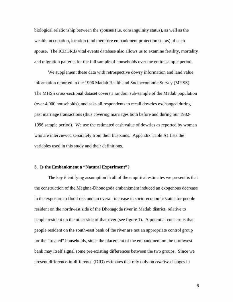
The key identifying assumption in all of the empirical estimates we present is that

the construction of the Meghna-Dhonogoda embankment induced an exogenous decrease

in the exposure to flood risk and an overall increase in socio-economic status for people

resident on the northwest side of the Dhonagoda river in Matlab district, relative to

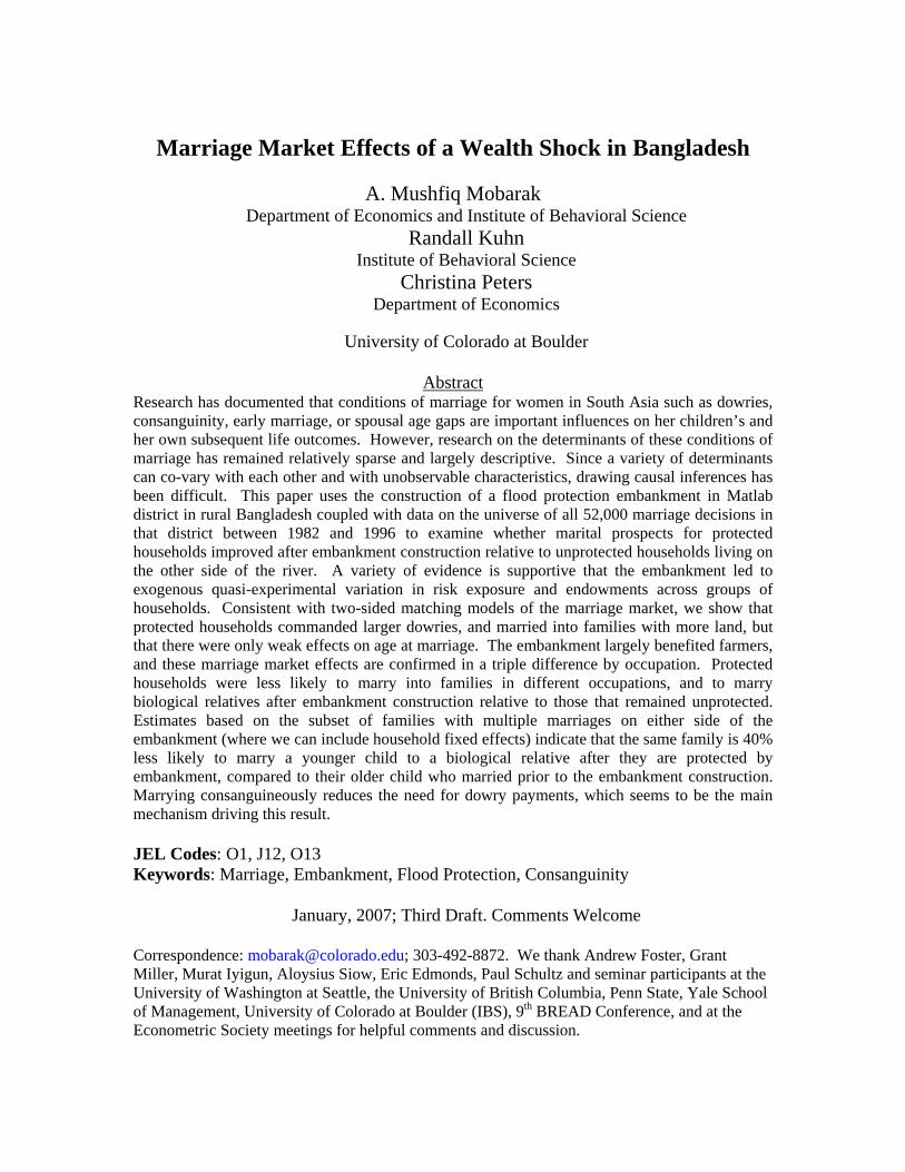
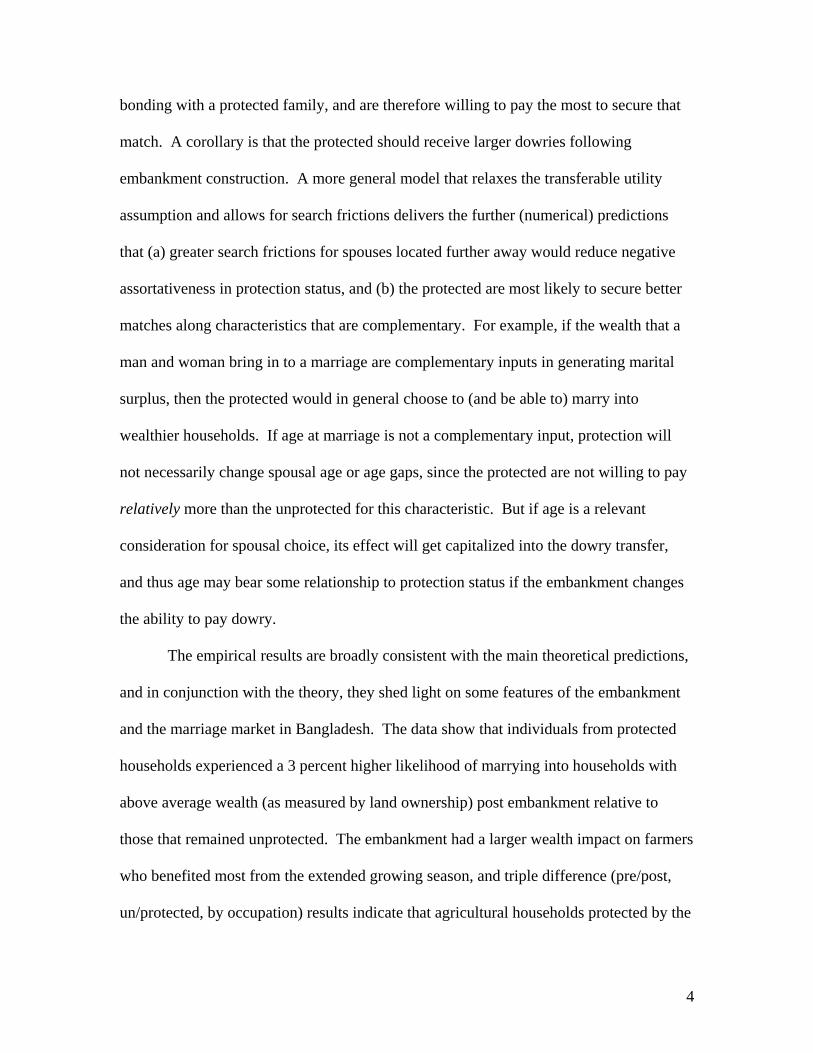
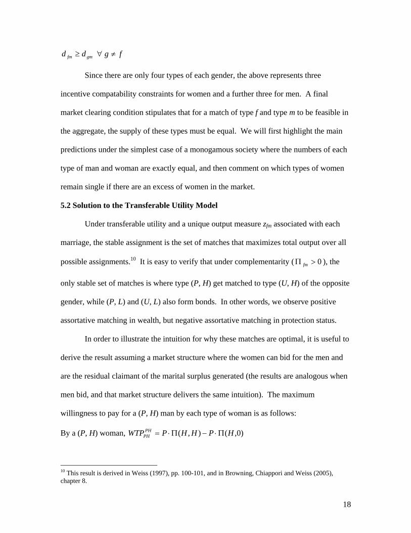
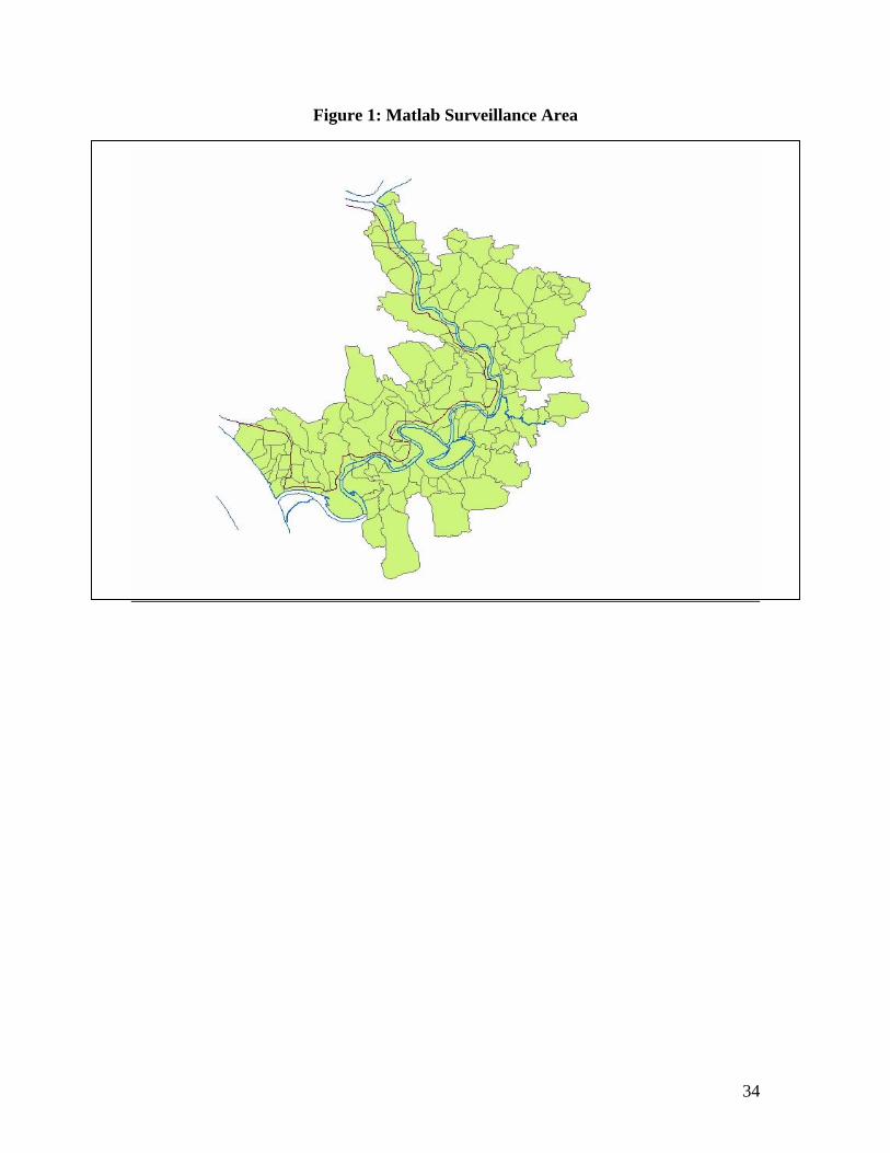
people resident on the other side of that river (see figure 1). A potential concern is that

people resident on the south-east bank of the river are not an appropriate control group

for the “treated” households, since the placement of the embankment on the northwest

bank may itself signal some pre-existing differences between the two groups. Since we

present difference-in-difference (DID) estimates that rely only on relative changes in

9

marriage outcomes between “treatment” and “control” households from pre to post

embankment construction, the most important concern is whether the temporal trends in

outcomes prior to the embankment were different across the two groups, and thus our

DID estimates merely report the continuation of such different pre-existing trends.

There are several ways to address these concerns. First, observable dimensions of

the composition of the protected and unprotected groups are similar prior to construction.

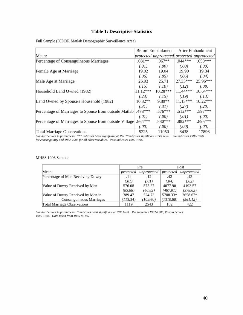
Descriptive statistics reported in Table 1 indicate that despite the fact that the marriage

outcomes of interest are often statistically different across the two groups prior to

completion of the embankment (due to the large sample), the magnitude of those

differences remains very small. One exception is the consanguinity rate, which is

appreciably larger prior to embankment construction on the protected side. In addition,

several program evaluations of the embankment project present evidence in support of

the homogeneity between protected and unprotected households before its construction

(Strong and Minkin, 1992; Thompson and Sultana, 1996). The geographic areas

experienced similar weather patterns, households grew similar crops and reported similar

incomes, and demographic distributions were nearly identical.5 Moreover, Thompson

and Sultana (1996) conclude that unprotected households are not affected by the

embankment or incidentally impacted by confinement of floodwaters to the unprotected

floodplain following embankment construction.

5 Since Matlab is part of a demographic surveillance area run by the International Centre for Diarrheal Disease Research (ICDDR, B), the population has been exposed to some development programs. The largest of these, The Matlab Maternal and Child Health and Family Planning program was implemented in a group of Matlab villages beginning in 1977, and an extension of this program (the Safe Motherhood Initiative) introduced to some of these villages in 1987. Our results are robust to controlling for exposure to these programs.

10

Second, although it is still possible that the two groups differ in unobservable

ways, anecdotal evidence from first-hand witnesses argue in favor of the embankment

placement as orthogonal to unobservable household characteristics or preferences related

to marriage market outcomes. For instance, John Briscoe (1998) observed members of a

village protected by the embankment, noting that the local people “were not consulted on

key [embankment] project decisions,” even when it concerns operation and maintenance

of the project ten years on. Kabir (2004) reaches a similar conclusion upon interviewing

local inhabitants across several villages who complain that the project was coordinated by

political leaders in conjunction with the largest local landowners who actually live in

Dhaka rather than Matlab. The marriage decisions of politicians and landowners resident

in Dhaka who may have influenced the placement of the embankment are not part of our

sample since they do not live in Matlab district. Conversations with Matlab residents

during fieldwork we conducted in December 2005 indicates that embankment was placed

on the north-west side mainly because drainage was worse in that bank prior to

embankment construction, which meant that agricultural fields would often be water-

logged, rendering the fields un-usable for up to 3-5 months per year.

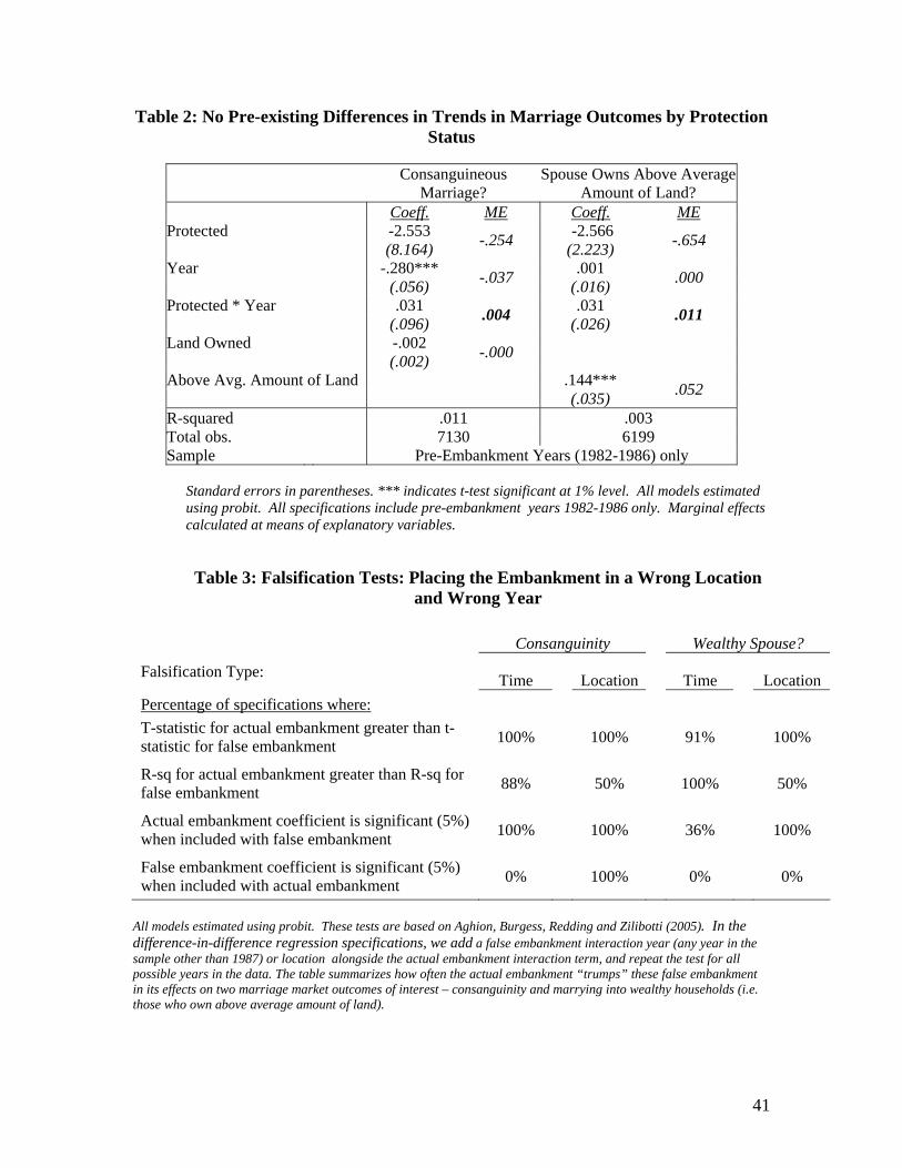
Third, we show that the pre-existing temporal trends in the marriage outcomes of

interest prior to embankment construction were not statistically different across the

protected and unprotected groups (see Table 2). Moreover, the marginal effects for these

insignificant differences are very small when compared with the actual embankment

effect estimates we present later. Any relative changes in trends post-embankment that

our difference-in-difference estimates uncover are therefore not merely a continuation of

pre-existing differences in trends.

11

We also conduct 2 types of falsification exercises in Table 3, modeled after

Aghion, Burgess, Redding and Zilibotti (2005). The first group of tests replaces the

indicator for the actual year of embankment construction with a false embankment year,

repeating the test for every possible false embankment year of the sample. The second

group of tests falsifies by location, and replaces the variable for protection status

(indicating which side of the embankment a household is on) with a false embankment

location. The first location pretends the embankment was built along a horizontal line

breaking villages into northern and southern groups. The second false location uses

placement of villages into treatment and control groups of the Matlab Maternal and Child

Health and Family Planning Program, an experimental program present in the area.

These tests for false times and locations all show that statistical impacts are absent in

cases where we should not observe them (e.g. there are no statistical differences in

behavior across two sub-periods other than that of embankment construction), and that

the actual embankment effect typically trumps the false embankment effects.

4. The First Order Impacts of the Embankment on Income and Risk

Frequent severe flooding creates problems in Matlab by contaminating the

submerged ground along with water and food supplies. The floods destroy subsistence

crops, inducing uncertainty and volatility in household income, and stagnant floodwaters

breed chronic diseases. The Meghna-Dhonogoda embankment protects the surrounding

land and population by providing a barrier along the waterway to prevent overflow,

consequently reducing the environmental risk experienced by the protected households.

In addition, the Bangladeshi government constructed systems for pumped drainage and

12

irrigation along the embankment, hoping to increase the agricultural seasons and resulting

crop yields for the area (Strong and Minkin, 1992).

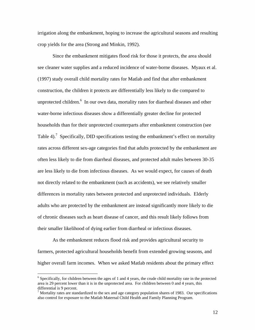
Since the embankment mitigates flood risk for those it protects, the area should

see cleaner water supplies and a reduced incidence of water-borne diseases. Myaux et al.

(1997) study overall child mortality rates for Matlab and find that after embankment

construction, the children it protects are differentially less likely to die compared to

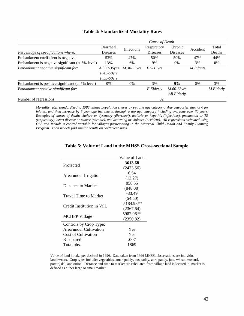
unprotected children.6 In our own data, mortality rates for diarrheal diseases and other

water-borne infectious diseases show a differentially greater decline for protected

households than for their unprotected counterparts after embankment construction (see

Table 4).7 Specifically, DID specifications testing the embankment’s effect on mortality

rates across different sex-age categories find that adults protected by the embankment are

often less likely to die from diarrheal diseases, and protected adult males between 30-35

are less likely to die from infectious diseases. As we would expect, for causes of death

not directly related to the embankment (such as accidents), we see relatively smaller

differences in mortality rates between protected and unprotected individuals. Elderly

adults who are protected by the embankment are instead significantly more likely to die

of chronic diseases such as heart disease of cancer, and this result likely follows from

their smaller likelihood of dying earlier from diarrheal or infectious diseases.

As the embankment reduces flood risk and provides agricultural security to

farmers, protected agricultural households benefit from extended growing seasons, and

higher overall farm incomes. When we asked Matlab residents about the primary effect

6 Specifically, for children between the ages of 1 and 4 years, the crude child mortality rate in the protected area is 29 percent lower than it is in the unprotected area. For children between 0 and 4 years, this differential is 9 percent. 7 Mortality rates are standardized to the sex and age category population shares of 1983. Our specifications also control for exposure to the Matlab Maternal Child Health and Family Planning Program.

13

of the embankment during fieldwork we conducted in December 2006, they were most

likely to report that it was their increased ability to take advantage of two to three crop

cycles per calendar year, rather than be limited to only one due to the fact that water

would encroach on the agricultural land for up to 3-5 months per year. We would thus

expect this wealth effect to be largest for farmers, although the effect may be somewhat

mitigated through an increase in irrigation requirements. The protection against

environmental risk that the embankment offers and the human capital effects of decreased

child mortality may confer a wealth effect on protected households engaged in all types

of occupations.

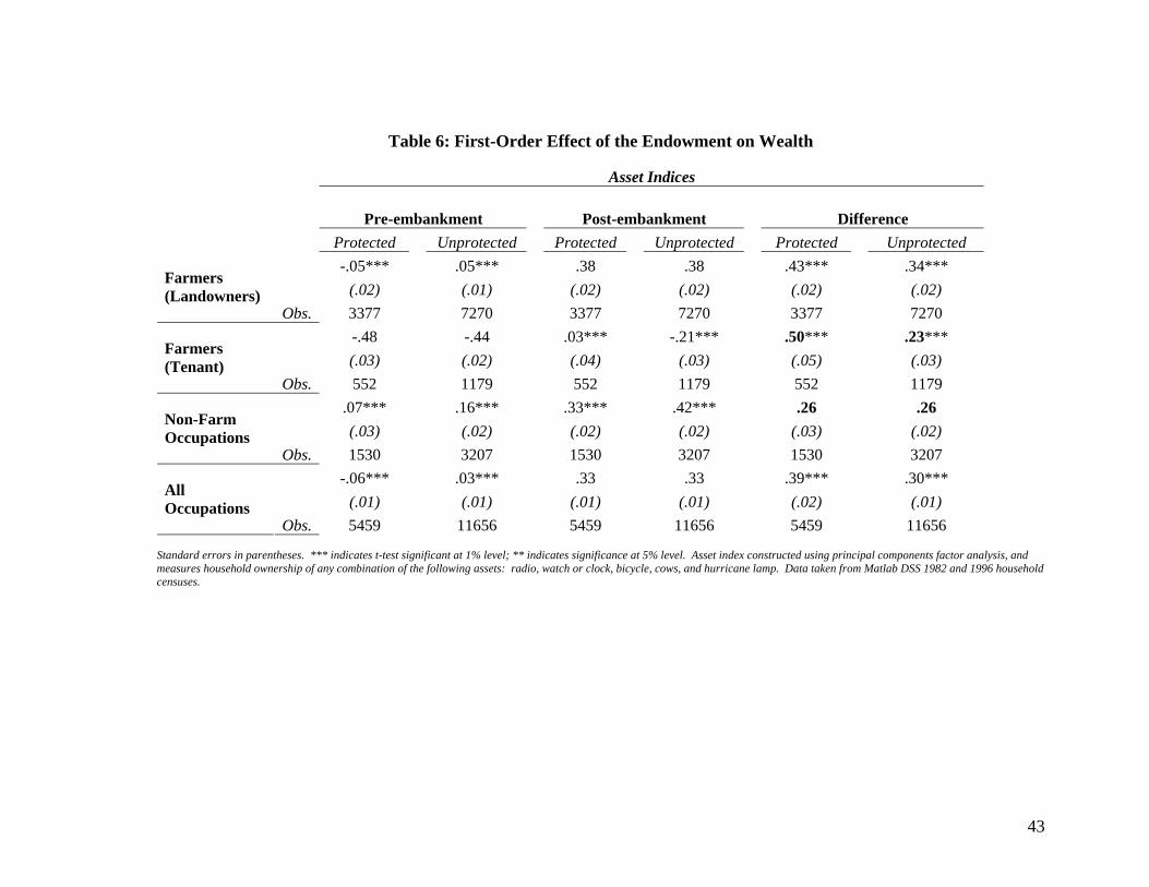
We measure the endowment effects directly by constructing asset indices for

household wealth in 1982 and 1996 using principal components factor analysis (see Table

6).8 Comparing asset indices of protected and unprotected households reveal that

protected households experience a differentially greater increase (significant at the 1

percent level) in asset ownership between 1982 (pre-embankment) and 1996 (post-

embankment). Moreover, this change is almost entirely driven by farmers, as expected.

Both landowners and tenant farmer benefited in significant ways, which indicates that the

extended growing season on the protected side probably increased both the productive

capacity of land as well as the demand for agricultural labor. A hedonic regression of the

value of land using the cross-sectional 1996 Matlab Health and Socio-Economic Survey

(MHSS) reveals that post-embankment, the unit price of land is higher on the protected

side (see table 5). Table 7 shows that the variance of assets across households within a

8 The index measures household ownership of any combination of the following assets: a radio, a watch or clock, a bicycle, cows, and a hurricane lamp. We compare asset indices for only those households with information in both 1982 and 1996. Occupation of household head is kept as reported in 1982 for all indices. Data is taken from Matlab DSS (Demographic Surveillance System) 1982 and 1996 household censuses.

14

village (which would be linked to changes in risk exposure) does not differentially

change across the protected or unprotected banks. Consistent with the field-work

findings, the mean wealth effect thus appears to dominate changes in variance.

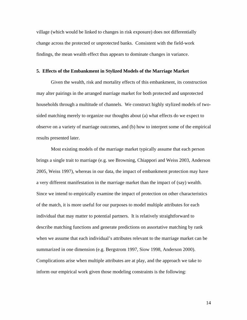
5. Effects of the Embankment in Stylized Models of the Marriage Market

Given the wealth, risk and mortality effects of this embankment, its construction

may alter pairings in the arranged marriage market for both protected and unprotected

households through a multitude of channels. We construct highly stylized models of two-

sided matching merely to organize our thoughts about (a) what effects do we expect to

observe on a variety of marriage outcomes, and (b) how to interpret some of the empirical

results presented later.

Most existing models of the marriage market typically assume that each person

brings a single trait to marriage (e.g. see Browning, Chiappori and Weiss 2003, Anderson

2005, Weiss 1997), whereas in our data, the impact of embankment protection may have

a very different manifestation in the marriage market than the impact of (say) wealth.

Since we intend to empirically examine the impact of protection on other characteristics

of the match, it is more useful for our purposes to model multiple attributes for each

individual that may matter to potential partners. It is relatively straightforward to

describe matching functions and generate predictions on assortative matching by rank

when we assume that each individual’s attributes relevant to the marriage market can be

summarized in one dimension (e.g. Bergstrom 1997, Siow 1998, Anderson 2000).

Complications arise when multiple attributes are at play, and the approach we take to

inform our empirical work given those modeling constraints is the following:

15

1. We derive some analytical predictions on matching in a simplified transferable-

utility marriage market where each person has only two discrete attributes –

embankment protection status and wealth status. We use this stylized market to

understand changes in equilibrium matches after the embankment is constructed

in cases where protection only contributes to wealth and where it confers both

wealth and risk mitigation benefits.

2. We then relax the assumptions on transferable utility, endow each person with

multiple continuous characteristics, and simulate stable matches in a much larger

marriage market characterized by search frictions.

We present the simplified analytical model first because it helps to clarify some of the

basic economic intuition behind the dynamics that we will observe later in the more

complicated simulated marriage market.

5.1 A Transferable Utility Model of the Marriage Market

Since marriages in Matlab are typically arranged by the families of the groom and

bride, we assume that preferences of the bride and her family are grouped together, as are

the preferences of the groom and his family. Males and females on the marriage market

are indexed by m and f. Each potential spouse has two relevant characteristics: their level

of wealth (wf or wm), which can be either high (H) or low (L), their embankment status (ef

or em), which can be either protected (P) or unprotected (U). Each marriage produces an

output zfm, and there exists a medium of exchange (such as a dowry payment in money,

which we denote dfm) that can be used to transfer utilities from the bride to the groom.

This is the transferable utility assumption commonly made in the marriage literature (e.g.

16

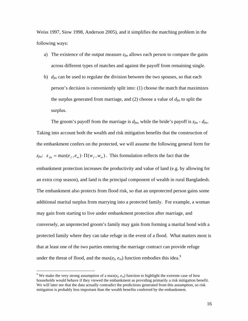
Weiss 1997, Siow 1998, Anderson 2005), and it simplifies the matching problem in the

following ways:

a) The existence of the output measure zfm allows each person to compare the gains

across different types of matches and against the payoff from remaining single.

b) dfm can be used to regulate the division between the two spouses, so that each

person’s decision is conveniently split into: (1) choose the match that maximizes

the surplus generated from marriage, and (2) choose a value of dfm to split the

surplus.

The groom’s payoff from the marriage is dfm, while the bride’s payoff is zfm - dfm.

Taking into account both the wealth and risk mitigation benefits that the construction of

the embankment confers on the protected, we will assume the following general form for

zfm: ),(),max( mfmffm wweez Π⋅= . This formulation reflects the fact that the

embankment protection increases the productivity and value of land (e.g. by allowing for

an extra crop season), and land is the principal component of wealth in rural Bangladesh.

The embankment also protects from flood risk, so that an unprotected person gains some

additional marital surplus from marrying into a protected family. For example, a woman

may gain from starting to live under embankment protection after marriage, and

conversely, an unprotected groom’s family may gain from forming a marital bond with a

protected family where they can take refuge in the event of a flood. What matters most is

that at least one of the two parties entering the marriage contract can provide refuge

under the threat of flood, and the max(ef, em) function embodies this idea.9

9 We make the very strong assumption of a max(ef, em) function to highlight the extreme case of how households would behave if they viewed the embankment as providing primarily a risk mitigation benefit. We will later see that the data actually contradict the predictions generated from this assumption, so risk mitigation is probably less important than the wealth benefits conferred by the embankment.

17

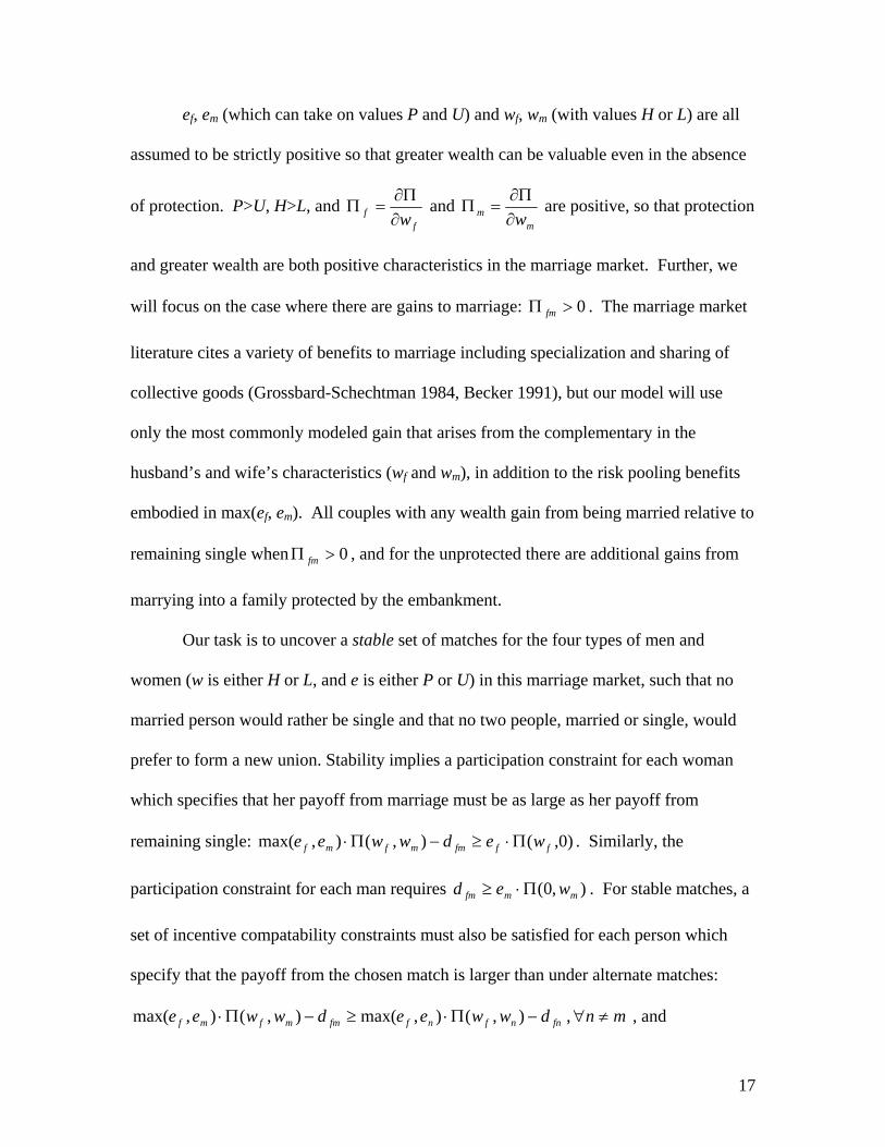
ef, em (which can take on values P and U) and wf, wm (with values H or L) are all

assumed to be strictly positive so that greater wealth can be valuable even in the absence

of protection. P>U, H>L, and f

f w∂Π∂

=Π and m

m w∂Π∂

=Π are positive, so that protection

and greater wealth are both positive characteristics in the marriage market. Further, we

will focus on the case where there are gains to marriage: 0>Π fm . The marriage market

literature cites a variety of benefits to marriage including specialization and sharing of

collective goods (Grossbard-Schechtman 1984, Becker 1991), but our model will use

only the most commonly modeled gain that arises from the complementary in the

husband’s and wife’s characteristics (wf and wm), in addition to the risk pooling benefits

embodied in max(ef, em). All couples with any wealth gain from being married relative to

remaining single when 0>Π fm , and for the unprotected there are additional gains from

marrying into a family protected by the embankment.

Our task is to uncover a stable set of matches for the four types of men and

women (w is either H or L, and e is either P or U) in this marriage market, such that no

married person would rather be single and that no two people, married or single, would

prefer to form a new union. Stability implies a participation constraint for each woman

which specifies that her payoff from marriage must be as large as her payoff from

remaining single: )0,(),(),max( fffmmfmf wedwwee Π⋅≥−Π⋅ . Similarly, the

participation constraint for each man requires ),0( mmfm wed Π⋅≥ . For stable matches, a

set of incentive compatability constraints must also be satisfied for each person which

specify that the payoff from the chosen match is larger than under alternate matches:

mndwweedwwee fnnfnffmmfmf ≠∀−Π⋅≥−Π⋅ , ),(),max(),(),max( , and

18

fgdd gmfm ≠∀≥

Since there are only four types of each gender, the above represents three

incentive compatability constraints for women and a further three for men. A final

market clearing condition stipulates that for a match of type f and type m to be feasible in

the aggregate, the supply of these types must be equal. We will first highlight the main

predictions under the simplest case of a monogamous society where the numbers of each

type of man and woman are exactly equal, and then comment on which types of women

remain single if there are an excess of women in the market.

5.2 Solution to the Transferable Utility Model

Under transferable utility and a unique output measure zfm associated with each

marriage, the stable assignment is the set of matches that maximizes total output over all

possible assignments.10 It is easy to verify that under complementarity ( 0>Π fm ), the

only stable set of matches is where type (P, H) get matched to type (U, H) of the opposite

gender, while (P, L) and (U, L) also form bonds. In other words, we observe positive

assortative matching in wealth, but negative assortative matching in protection status.

In order to illustrate the intuition for why these matches are optimal, it is useful to

derive the result assuming a market structure where the women can bid for the men and

are the residual claimant of the marital surplus generated (the results are analogous when

men bid, and that market structure delivers the same intuition). The maximum

willingness to pay for a (P, H) man by each type of woman is as follows:

By a (P, H) woman, )0,(),( HPHHPWTP PHPH Π⋅−Π⋅=

10 This result is derived in Weiss (1997), pp. 100-101, and in Browning, Chiappori and Weiss (2005), chapter 8.

19

By a (P, L) woman, )0,(),( LPHLPWTP PHPL Π⋅−Π⋅=

By a (U, H) woman, )0,(),( HUHHPWTP PHUH Π⋅−Π⋅=

By a (U, L) woman, )0,(),( LUHLPWTP PHUL Π⋅−Π⋅=

Since P>U, PHPH

PHUH WTPWTP > and PH

PLPH

UL WTPWTP > . This is simply because a

protected man offers greater value added to an unprotected woman than he does to a

protected woman, and the unprotected woman will therefore be willing to outbid the

protected woman. Also, PHUL

PHUH WTPWTP > when 0>Πmf . Under complementarity in

the husband’s and wife’s wealth, a high wealth woman gains greater surplus from a high

wealth man than does a low wealth woman, and will therefore be willing to outbid her.

Thus the (U, H) woman can outbid all other types of women in order to match with a (P,

H) man.

The above implies that a (P, H) man will be feasible for a (U, H) woman, but in

order to show that this is the match that will occur in equilibrium, we also need to

demonstrate that the (U, H) woman wants the (P, H) man – that a marriage to this man

generates more surplus for her than a marriage to any other man. If the (P, H) - (U, H)

match is surplus maximizing, then we can find a transfer dfm such that the (U, H) woman

and (P, H) man are better off under this match than under any other pairing. This is

easily established, as we can use the assumptions P>U, 0>Πm , 0>Π f , and 0>Π fm to

show that PHUHWTP exceeds PL

UHWTP , UHUHWTP , and UL

UHWTP .

Analogous arguments establish that (P, H) type women have the highest

willingness to pay for (U, H) type men, and achieve the largest surplus from those

matches. So for both men and women, all matches are of the form (P, H) - (U, H). Once

20

all these (P, H) - (U, H) men and women are paired up (and if there are an equal number

of them, all of them disappear from the market), of the remaining women in the market,

(U, L) types place the highest bid for (P, L) men, and they are also their surplus

maximizing choice. So the remaining matches for both men and women are of the form

(P, L) - (U, L). Note that H-type women can typically outbid L-type women, and if there

are an excess of H-type women (over H-type men) in the market, then we will observe

some (U, H) women marrying (P, L) men (and (P, H) marrying (U, L)), which will in turn

force some L-type women to remain single.

The general result highlighted by this model is that we should observe positive

assortative matching in men’s and women’s characteristics that are complements and

negative assortative matching in characteristics that are substitutes. If the primary role of

the embankment is risk mitigation, then after embankment construction we should

observe more marriages contracted between families living on opposite banks of the

river. In reality there are important search frictions in marriage markets, and the market

in Matlab district is highly localized where the majority of matches are between families

located closer together (i.e. on the same bank). Thus the risk mitigation benefits of the

embankment would have to be strong enough to overcome these search frictions for us to

observe negative assortative matching along protection status following embankment

construction. Further, to the extent that the embankment confers any positive wealth or

health benefits that are complementary,11 there may also be some positive assortative pull

to protection status.

11 For example, it could be that the marginal returns to women’s health for her children’s outcomes is larger when her husband is more likely to survive and be healthy. The zfm function we postulate in the previous section highlights the risk mitigation benefits of embankment protection and this is modeled as a substitute

21

Although the transfer payments from wives to husbands are not precisely pinned

down in the general model (the participation and incentive compatability constraints only

place upper and lower bounds on the feasible values of dfm), we can study changes in

dowries following embankment construction under specific market structures, such as the

case where women bid for men in a multi-unit English auction setting. If there are

multiple (U, H) women bidding for the same (P, H) man, the women would compete

away the entire surplus generated by this man, and dowry payments would increase with

protection status after embankment construction, since the man’s contribution to the total

marital surplus increases with his protection status.

5.3 Embankment Effects in a Simulated Gale and Shapley (1962) Matching Model

We now relax a number of the restrictive assumptions made in the model outlined

above and simulate marriages in a more general model. Potential spouses can offer

compensating differentials along multiple dimensions in order to secure a desirable match

in the arranged marriage market. For example, a family could make up any deficiency in

its relative wealth position by offering their candidate at the age most desirable by the

opposite sex, or accepting a candidate of a less desirable age, or accepting a lower dowry

payment. We now study the dynamics of matching in a marriage market where each

candidate is endowed with a continuous characteristic that is complementary to

embankment protection (such as the amount of land or wealth), another continuous

characteristic relevant to spousal choice which is neither a complement nor a substitute to

protection (age at marriage), a discrete protection status, and an idiosyncratic

characteristic, but if the embankment is strictly wealth enhancing, so that ),( mmfffm ewewz ++Π= , we may observe positive assortative matching along protection status.

22

attractiveness parameter. A male m’s payoff from marrying a female f is postulated to be:

[ ] fmffmfmf

fm aawwees εβα +−−+Π⋅= 2* )(),(),max( (1)

e is embankment protection status, w is wealth, a is age, *fa (a constant) is the most

desired female age at marriage (from a man’s perspective), fmε is the idiosyncratic pair-

specific attractiveness parameter that measures male m’s preference for female f, and α

and β are constants. Greater wealth and protection status are considered attractive

characteristics in the marriage market, and as before, the husband’s and wife’s wealth,

and protection status are complementary inputs (e.g. protection extends the crop growing

season and increases the productivity of land). The insurance (i.e. reduced risk exposure)

benefits of the embankment make the husband’s and wife’s protection status substitutes.

Candidates are penalized if their age at marriage differs from some optimal age at

marriage.

A female f’s payoff from marrying male m is postulated to be:

[ ] mfmmmfmf

mf aawwees εβα +−−+Π⋅= 2* )(),(),max( (2)

For male m, (1) defines a scoring function over all women that he can use to

evaluate whom to propose to and marry. Similarly, (2) defines a scoring function for

female f over all men. If there are a total of M men and F women on the market, given

each man and woman’s characteristics, we can use (1) and (2) to define an M x F matrix

of scores over all men and women. We could then use the Gale and Shapley (1962)

algorithm to identify the stable set of matches in this market of M men and F women.12

12 The seminal Gale and Shapley matching algorithm is described in Gale and Shapley (1962). This algorithm, where men propose their most preferred woman, and the woman holds on to the most attractive man while rejecting the rest, and the men then propose to their next best option, and so on …, produces a

23

A simple way to add search frictions to this model is to assume that individuals are more

likely to see (and propose to) others on the market who are physically closer to them.

Since we cannot describe analytical solutions to the matches that occur in this

algorithm, we simulate the matches by endowing 2500 men and 2500 women with a

distribution of wealth, age, protection and attractiveness characteristics. We assume that

initially each individual gets an independent draw on wealth from a truncated normal

distribution over positive support, a draw on age from a uniform distribution (on support

16-22 for women with an optimal age at marriage, *fa of 19, and on support 21-27 for

men, with *ma =24), and a draw on preferences for each individual of the opposite gender

from a normal (0,1) distribution. Half of all men and all women are randomly assigned to

each bank of the river, and an embankment is constructed on only one side of the river.

We assume a monogamous society where men propose. The probability that a man

“sees” a woman residing on the same side of river on the marriage market is qb and the

probability that he sees a woman on the opposite bank is qs with qb > qs. Search frictions

are larger the lower the values of qb and qs.

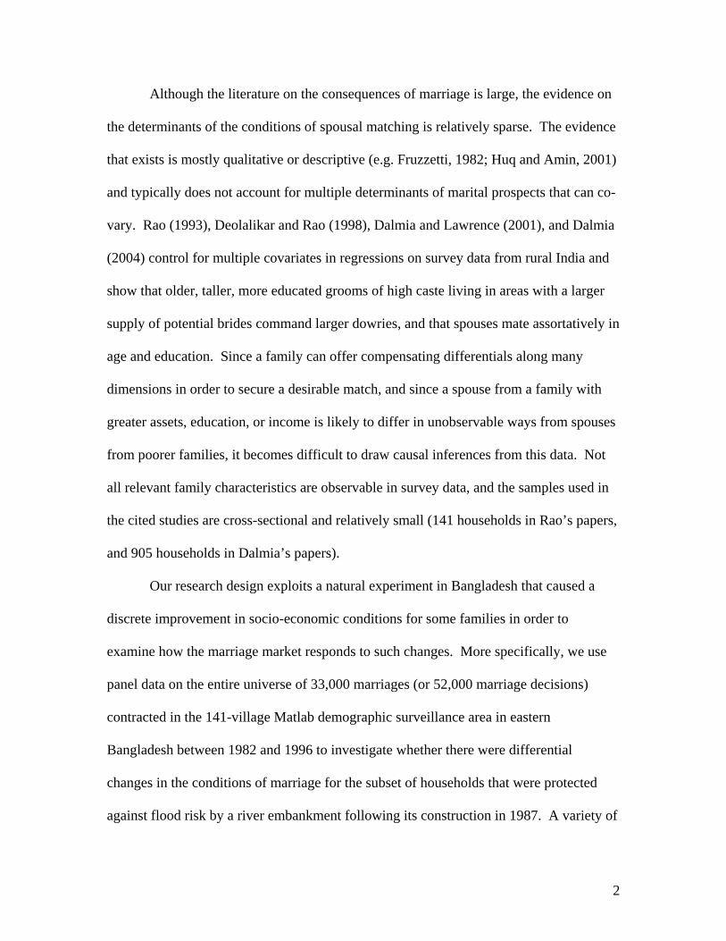
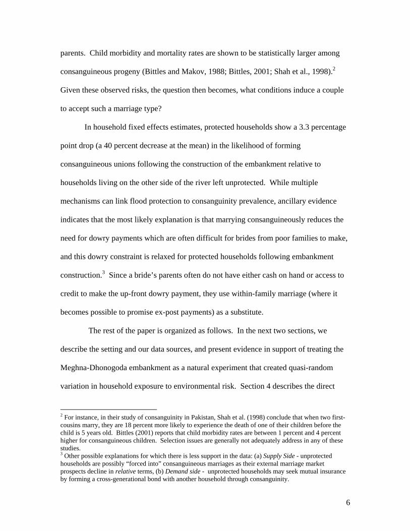
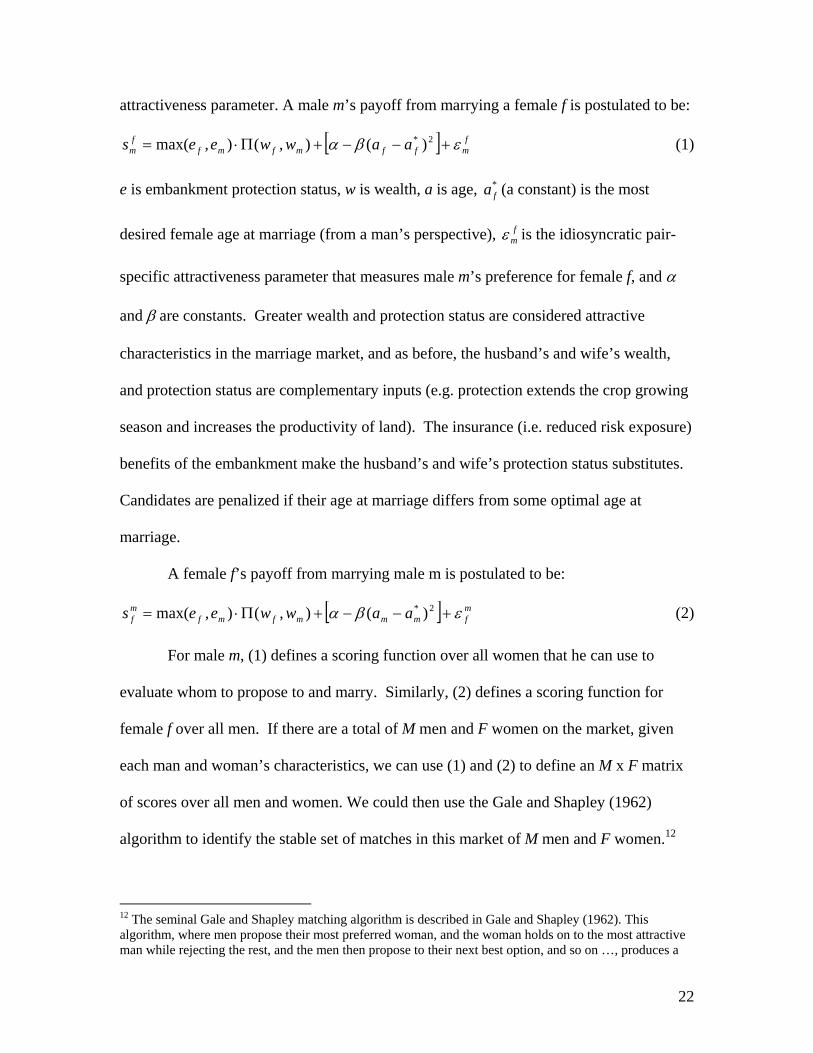
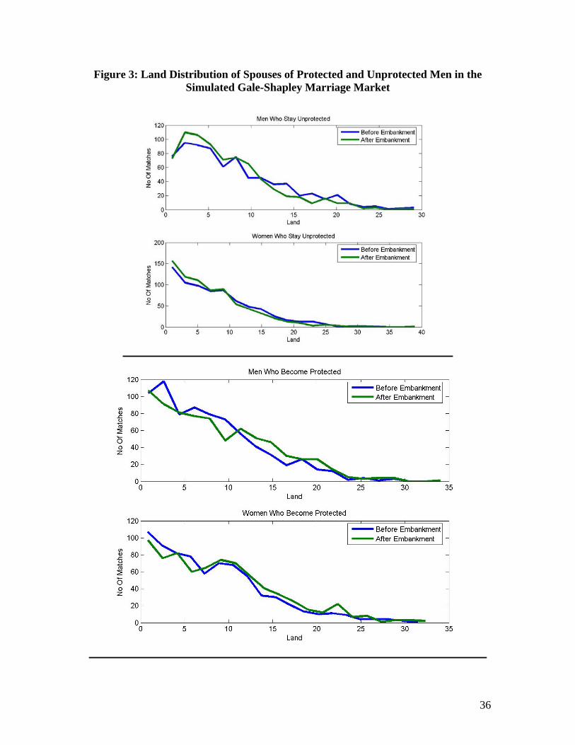
Results of the matching simulation are summarized in figures 3-6. Figure 3

shows that for both protected men and women, the wealth (land) distribution of spouses

they match with shifts to the right following embankment construction. Conversely, the

wealth distribution of spouses shifts to the left for men and women on the other bank of

the river (who remain unprotected) following embankment construction. Thus, the

protected are able to secure wealthier spouses at the expense of the unprotected.

Individuals residing on the two sides of the river are in direct competition in the marriage

stable set of matches where no two man and woman not paired to each other through the algorithm would be better off by contracting that marriage.

24

market, and this result comes about because (a) the protected have an extra desirable

characteristic to offer, so their offers are more likely to be accepted and (b) due to

complementarity in protection status and land, they are more likely to extend offers of

marriage to higher-wealth individuals.

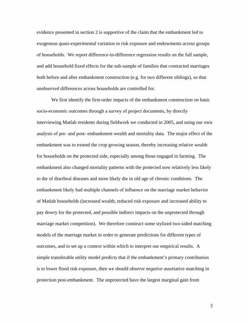
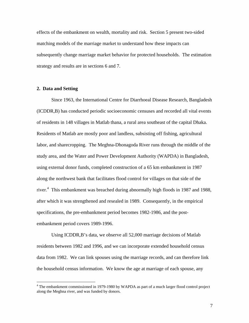
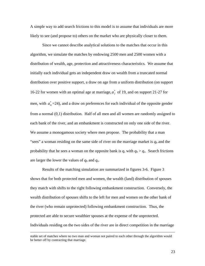
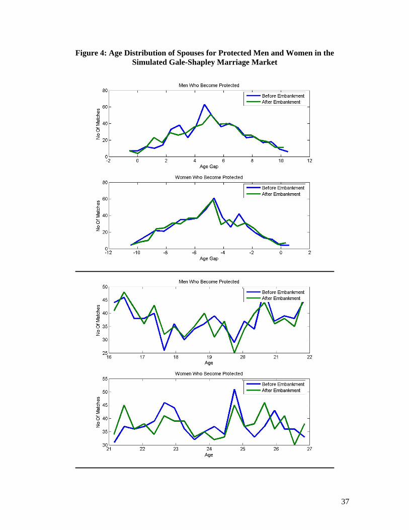
For age at marriage, where no such complementarity exists, figure 4 shows that

there no clear trend to indicate that the protected are better able to secure partners at the

“optimal” age, or reduce spousal age gaps. Complementarity in inputs is therefore key to

understanding the potential impacts of the embankment construction on the variety of

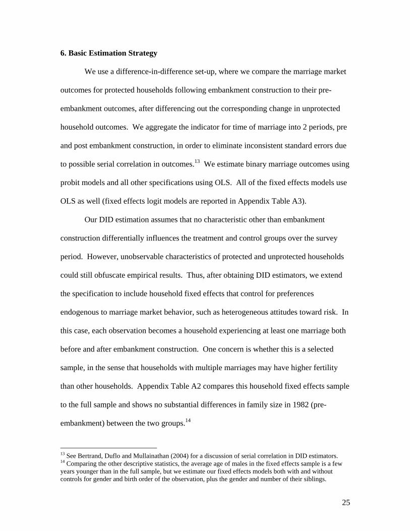
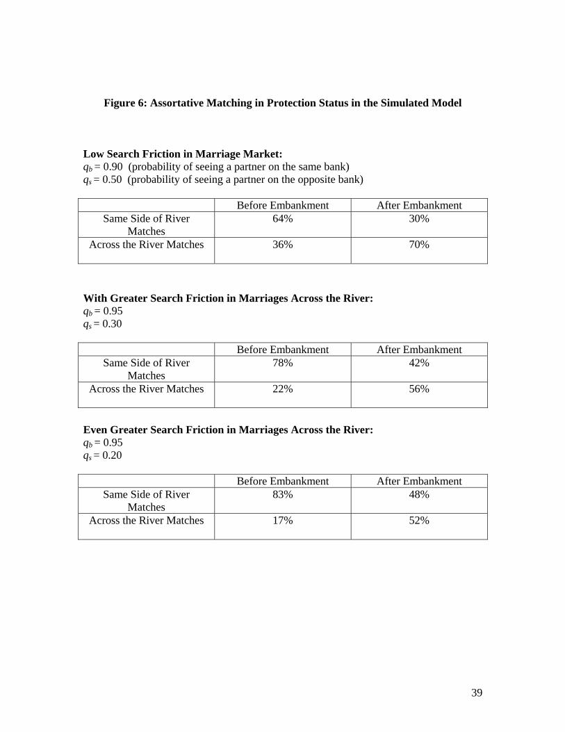
possible marriage market outcomes. The model also exhibits negative assortative

matching in the substitute characteristic – protection status. Within-bank marriages are

less likely to occur after embankment construction, but this effect is mitigated when the

levels of search friction are greater (see figure 6).

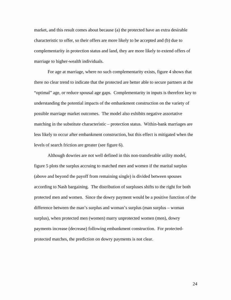
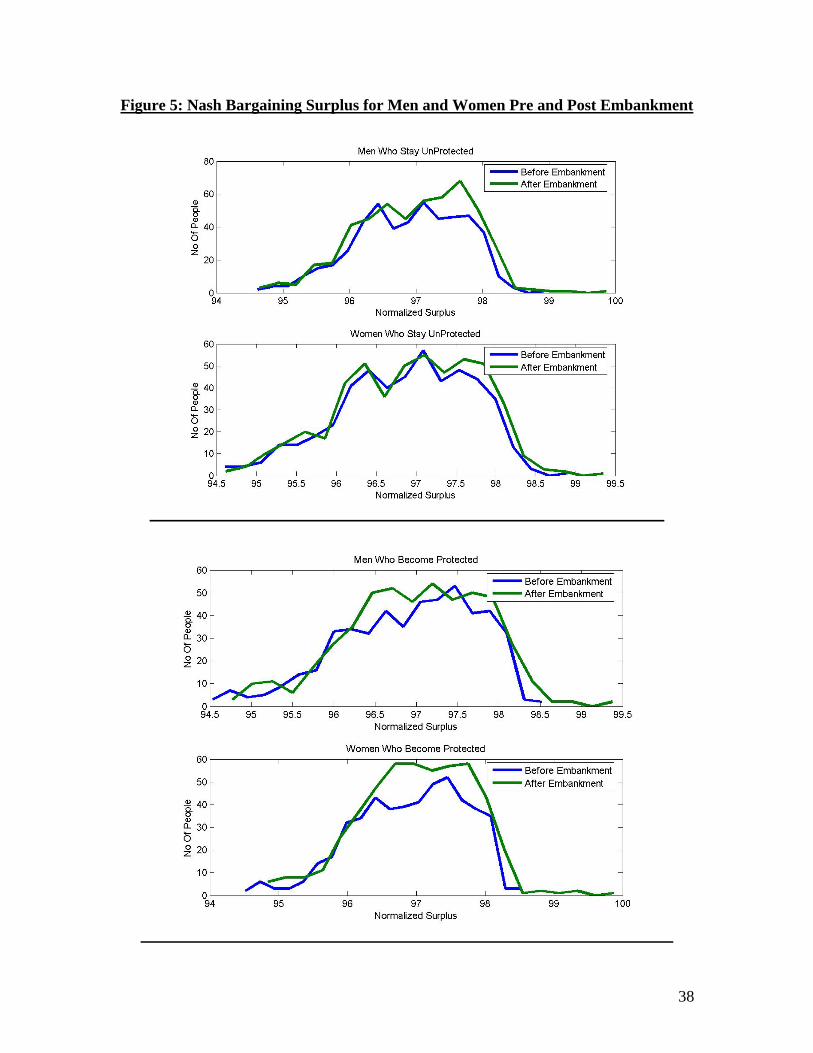
Although dowries are not well defined in this non-transferable utility model,

figure 5 plots the surplus accruing to matched men and women if the marital surplus

(above and beyond the payoff from remaining single) is divided between spouses

according to Nash bargaining. The distribution of surpluses shifts to the right for both

protected men and women. Since the dowry payment would be a positive function of the

difference between the man’s surplus and woman’s surplus (man surplus – woman

surplus), when protected men (women) marry unprotected women (men), dowry

payments increase (decrease) following embankment construction. For protected-

protected matches, the prediction on dowry payments is not clear.

25

6. Basic Estimation Strategy

We use a difference-in-difference set-up, where we compare the marriage market

outcomes for protected households following embankment construction to their pre-

embankment outcomes, after differencing out the corresponding change in unprotected

household outcomes. We aggregate the indicator for time of marriage into 2 periods, pre

and post embankment construction, in order to eliminate inconsistent standard errors due

to possible serial correlation in outcomes.13 We estimate binary marriage outcomes using

probit models and all other specifications using OLS. All of the fixed effects models use

OLS as well (fixed effects logit models are reported in Appendix Table A3).

Our DID estimation assumes that no characteristic other than embankment

construction differentially influences the treatment and control groups over the survey

period. However, unobservable characteristics of protected and unprotected households

could still obfuscate empirical results. Thus, after obtaining DID estimators, we extend

the specification to include household fixed effects that control for preferences

endogenous to marriage market behavior, such as heterogeneous attitudes toward risk. In

this case, each observation becomes a household experiencing at least one marriage both

before and after embankment construction. One concern is whether this is a selected

sample, in the sense that households with multiple marriages may have higher fertility

than other households. Appendix Table A2 compares this household fixed effects sample

to the full sample and shows no substantial differences in family size in 1982 (pre-

embankment) between the two groups.14

13 See Bertrand, Duflo and Mullainathan (2004) for a discussion of serial correlation in DID estimators. 14 Comparing the other descriptive statistics, the average age of males in the fixed effects sample is a few years younger than in the full sample, but we estimate our fixed effects models both with and without controls for gender and birth order of the observation, plus the gender and number of their siblings.

26

7. Results

7.1 Household Responses to Changes in Risk Exposure

We first examine whether households view this embankment as primarily altering

their exposure to flood risk, and respond by changing their marriage patterns. For risk

averse individuals the embankment may lower their demand for mitigating risk through

other channels (e.g. marrying daughters into geographically distant households not

subject to the same weather patterns or planting different crops, a la Rosenzweig and

Stark, 1989). We would then expect to see changes in female migration patterns for

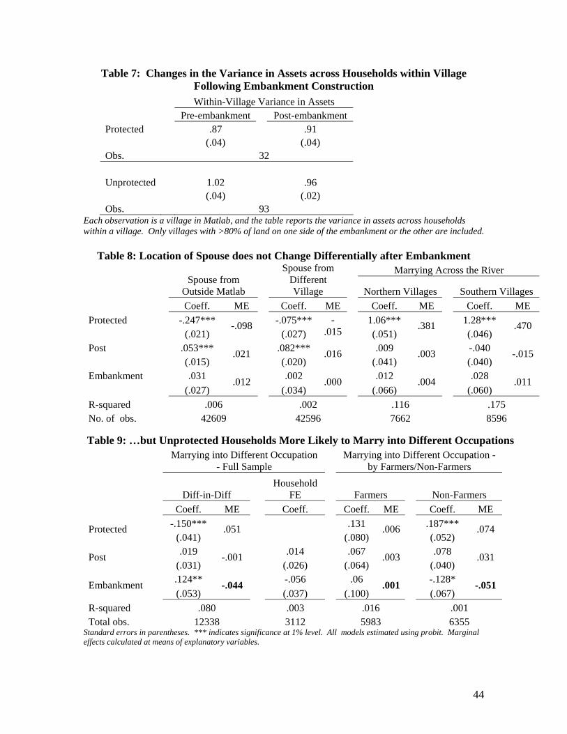
marriage following embankment construction. We test this hypothesis by looking at the

embankment’s effect on female marriage migration patterns both into households outside

their own villages as well as into households outside the Matlab area. The difference-in-

difference results from Table 8 find no evidence of such behavior, in that marriage

migration rates following embankment construction do not differentially change for

women from protected households when compared with unprotected women.

Further, the theoretical model outlined in section 5 showed that if risk mitigation

benefits of the embankment were an important consideration, then we would expect to

see negative assortative matching in protection status. The last two columns of table 8

(and the last column of table 12) show that there is no evidence of assortative matching

by embankment protection in either direction.15 In general, households are much more

likely to marry others who are located closer to them (see the coefficients on “protected”

in table 8), an indication of search frictions in the marriage market, but this propensity

15 Given the occupational distribution in villages across Matlab district, households are more likely to enter marriage contracts with different types of households when marrying across the river in southern villages, but the last two columns of table 8 show that households in the north and south do not behave any differently in terms of marrying across the river following embankment construction.

27

does not change after embankment construction. This highlights the fact that empirical

results on assortative matching based on cross-sectional data may be uninformative, since

it is difficult to separate out search frictions from assortative matching in cross-sectional

data.

In Table 9, we do find that protected households become 4-5 percentage points

less likely to marry into different occupations following embankment construction, an

indication that some households use the marriage market to diversify income risk. This

result may merely indicate assortative matching in wealth rather than response to risk if

the correlation is driven by rich protected farmers marrying other rich protected farmers

following embankment construction. However, the last two columns indicate that this is

not the case – that the correlation is entirely driven by households engaged in non-

farming occupations.

7.2 Household Responses to the Wealth Shock

If protected households become wealthier following embankment construction

and can offer “protection” as a desirable marriage market characteristic, then the

matching model predicts that such households would seek out better spousal

characteristics that are complementary to their own in producing marital surplus (e.g.

socio-economic status), but not necessarily characteristics which are not complementary.

Since land acts as the primary form of wealth for Matlab households, we measure a

spouse’s socio-economic status according to the amount of land owned by the head of the

household in 1982.16 We also look for effects on changes on age at marriage and spousal

age gaps.

16 Our data observes the amount of land owned by a household only if it lies within the surveillance area, and so this specification cannot include any household marrying outside Matlab (e.g. a migrant marriage

28

Protected households are more likely to marry into households with above

average amounts of land after embankment construction relative to the unprotected (see

Table 9). Protected households exhibit a 3 percentage point increase in their ability to

marry into households with an amount of land greater than the mean (a 10 percentage

point increase given their pre-embankment likelihood of 32 percent). The direction of

this change is robust to controlling for household fixed effects, although the effect

becomes statistically weaker when the identification comes from multiple marriages

before and after embankment construction in the same household. Furthermore, the

effects are confirmed in a triple difference in table 14, in that the result on marrying into

wealthier households is entirely driven by protected farmers, who are primary

beneficiaries of embankment construction, and the group that experienced the largest gain

in assets between 1982 and 1996. Protected farmers (who form 58% of our sample) have

a 5.3 percentage point increase in the propensity to marry into wealthy households (a

16% increase at the mean) following embankment construction relative to unprotected

farmers, whereas the effect among non-farmers is essentially zero.

In order to establish that our results are not crucially dependent on data from the

years farthest after embankment construction, we include alongside each model an

alternate specification that eliminates the last three years of the sample (the post-

embankment years then become 1989-1993). Limiting the sample in this way does not

alter the results (in fact, makes them stronger), supporting embankment construction as

the cause of a discrete one-time change in socio-economic conditions for protected

households.

household). The marriage migration results discussed earlier do not find evidence of differential post-embankment marriage migration rates between protected and unprotected households (see Table 8), a sample excluding these migrants should not yield biased estimates of the embankment effect.

29

We next examine the embankment’s impact on age at marriage and spousal age

gaps. There is weak evidence that both protected men and women are able to

differentially delay marriage, but these age effects are statistically indistinguishable from

zero. Consistent with the theoretical model, we find no impact of the embankment on

either age at marriage or spousal age gaps.

7.3 Effects on Consanguinity

Although the biological and genetic risks for the offspring of the union of

biologically close relatives are well understood in the scientific community,

consanguineous marriages remain common practice in much of the developing world,

and is as high as 50% of all marriages in Pakistan and Iraq. While the rates of

consanguinity are dropping over time in both protected and unprotected households in

Matlab, table 12 shows the drop is much larger among protected households after the

embankment is built. In the difference-in-difference, protected households are 2.5

percentage points less likely to marry a biological relative (i.e. second cousin or closer)

after the embankment over and above the change among the unprotected. In the

household fixed effects specification, we find that the same family is 40% (about 3

percentage points) less likely to marry a younger child to a biological relative after they

are protected by embankment, than their older child who married prior to the

embankment construction

There are several possible conceptual links between the embankment and rates of

consanguinity. If consanguinity is an inferior marriage outcome, protected households,

with the additional attractive characteristic they can offer on the marriage market, may be

more likely to avoid this outcome. Consanguinity may also be a response to risk

30

exposure in that households prefer to marry cousins in order to form robust inter-

generational bonds with the extended family. Finally, it has been postulated that

households marry within the family in South Asia in order to avoid large dowry payments

at the time of marriage (Caldwell et al. 1983; Bittles 1994). This last link is actually a

little more complicated, since one must explain why a rational male would forego larger

dowry payments in the outside market in order to marry his female cousin. Although the

MHSS data shows that the dowry transfer at the time of marriage is much smaller in

consanguineous unions (see table 13), conversations with Matlab residents during our

fieldwork indicated the total amount of effective dowry transfer over the course of the

marriage may not be any different. Consanguinity appears to act as a substitute for the

credit market. Credit constrained households who cannot borrow to pay dowries at the

time of marriage may use consanguinity as a way to delay payments. The promise to pay

over a longer period is more credible when made within the family.

There is substantial ancillary evidence in favor of the credit constraint story above

as one main motivation for consanguinity that explains its link to the embankment. The

embankment, by increasing wealth on the protected side, relaxed the dowry payment-in-

advance constraint, taking away this important motivation for marrying within the family.

We first show that the dowry transfer at the time of marriage is almost 50% lower in

consanguineous unions. Second, we show that the drop in consanguinity following

embankment construction is much larger among protected females than among protected

males. Since dowries are paid by the brides’ families (and not the grooms’), then we can

take advantage of a triple difference by gender, since we would expect consanguinity

rates to drop among protected females relatively more than males if the dowry payment

31

and credit constraint story is correct. The same protected family is upto 4.7 percentage

points less likely to marry their younger daughter to her cousin after embankment

construction relative to her older sibling, while for males, this drop is only about half as

large (see table 15).

7.4 Effect on Dowries and some other Specification checks

Tobit models in Table 13 use retrospective dowry information from all married

residents interviewed in the 1996 MHSS data, where we regress each woman’s report of

dowry payment as a function of husband’s embankment protection status. Comparing the

“Protected Husband” and “Year*Protected” coefficients, we see that protected men start

receiving larger dowries than unprotected men in 1989 or 1990 (the beginning of the

post-embankment period) for all specifications.

As a robustness check, we test that our results are not generated by the

endogenous sorting of households around the embankment as they migrate to protected

areas or away from the area altogether following its construction. 5 percent of our

sample migrates to another area in Matlab during the post-embankment period for a

reason other than marriage, and re-estimating the models without these migrants does not

qualitatively change the results (see Appendix Table A4).17 In addition, a second

robustness check shows our results to be insensitive to exclusion of marriage

observations that end in divorce.

8. Conclusion

In the last several decades, flood protection projects have become a popular tool

on the agenda of many developing countries. In Bangladesh alone, the government

17 In addition, Strong and Minkin (1992) analyze migration data before and after construction to conclude that there exist no real changes in outmigration rates for either the protected or unprotected areas.

32

completed 437 protection projects between 1954 and 1990, including the construction of

over 7555 kilometers of river embankments (Thompson and Sultana, 1996). Taken

together, these projects protect nearly a quarter of the country’s land, irrigating a half

million hectares and guarding an estimated 30 million people. If governments wish to

assess the full benefits and costs of disaster protection, it is imperative to understand how

household decision-making responds to these projects.

The existing literature focuses on the direct impacts of disaster mitigation

measures, elucidating how they affect ecosystem equilibrium, agricultural practices and

incomes, and the health of the surrounding population (e.g. Haque and Zaman, 1993;

Myaux et al., 1997; Paul, 1995; Thompson and Sultana, 1996). However, the literature

remains strikingly silent regarding any long-term indirect impacts of these measures on

household behavior. Our results complement this work by highlighting some long-term

shifts in household behavior following a change in environmental risk exposure. The

behavioral changes with respect to the marriage market that we document are in an

important sphere of their lives that can have even longer-term inter-generational

consequences.

Consistent with both transferable utility and non-transferable utility models of the

marriage market, we see that embankment-protected households who are able to offer

this as an attractive characteristic on the marriage market secure better marriage matches

in a characteristic that is complementary in generating marital surplus (socio-economic

status) but not a characteristic that is independent (age at marriage). The empirical

analysis, coupled with the theory, allows us to distinguish between the wealth and risk

mitigation benefits of the embankment. Households appear to respond primarily to the

33

wealth gains in their marriage market behavior, although there is some evidence that

Matlab households use marriage to diversify income risk. The practice of marrying

biological relatives appears to be closely linked to the institution of dowry. Rural

Bangladeshi households engage in consanguinity in response to the absence of credit for

paying dowries at the time of marriage.

These improvements in the conditions of marriage that we document for

households protected by the embankment can have even longer-term inter-generational

consequences due to their impact on both female and child socioeconomic outcomes.

34

Figure 1: Matlab Surveillance Area

35

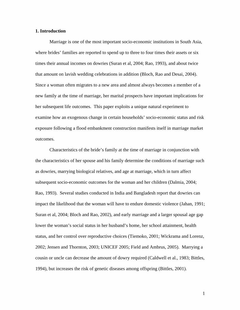
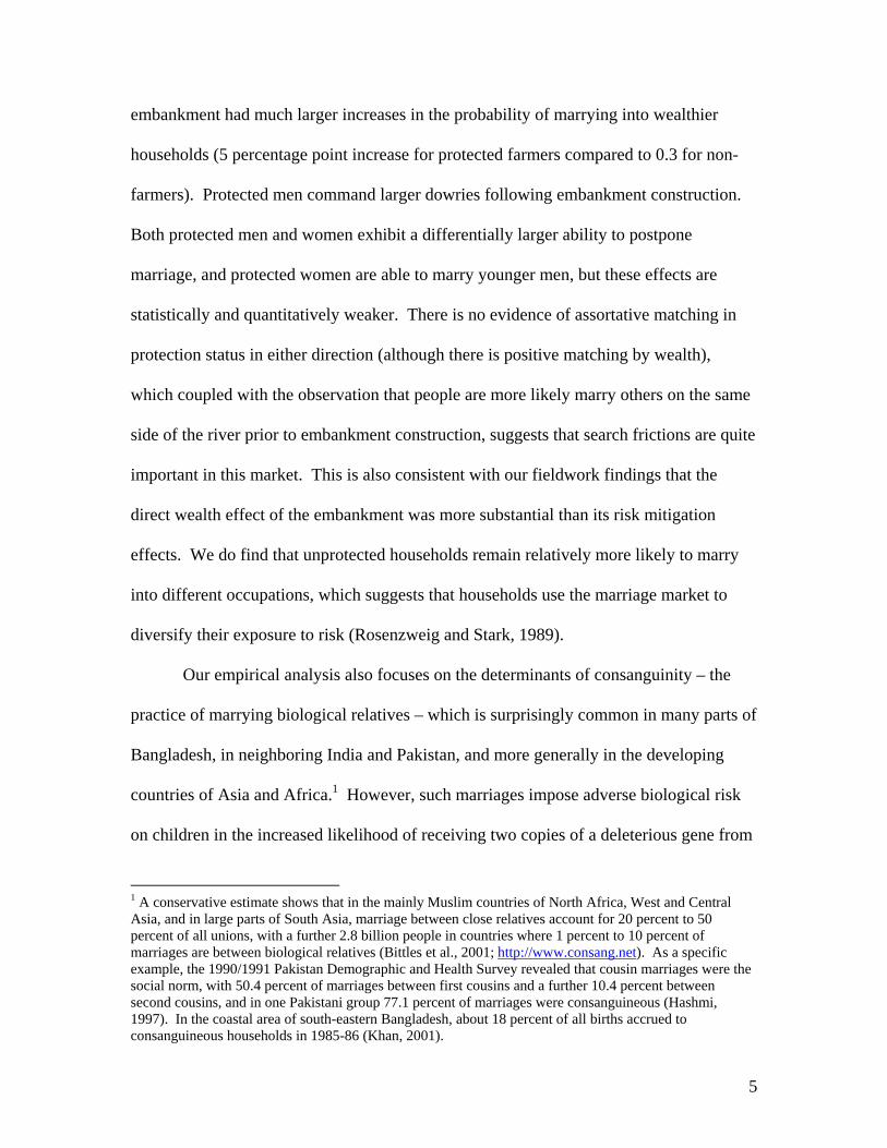
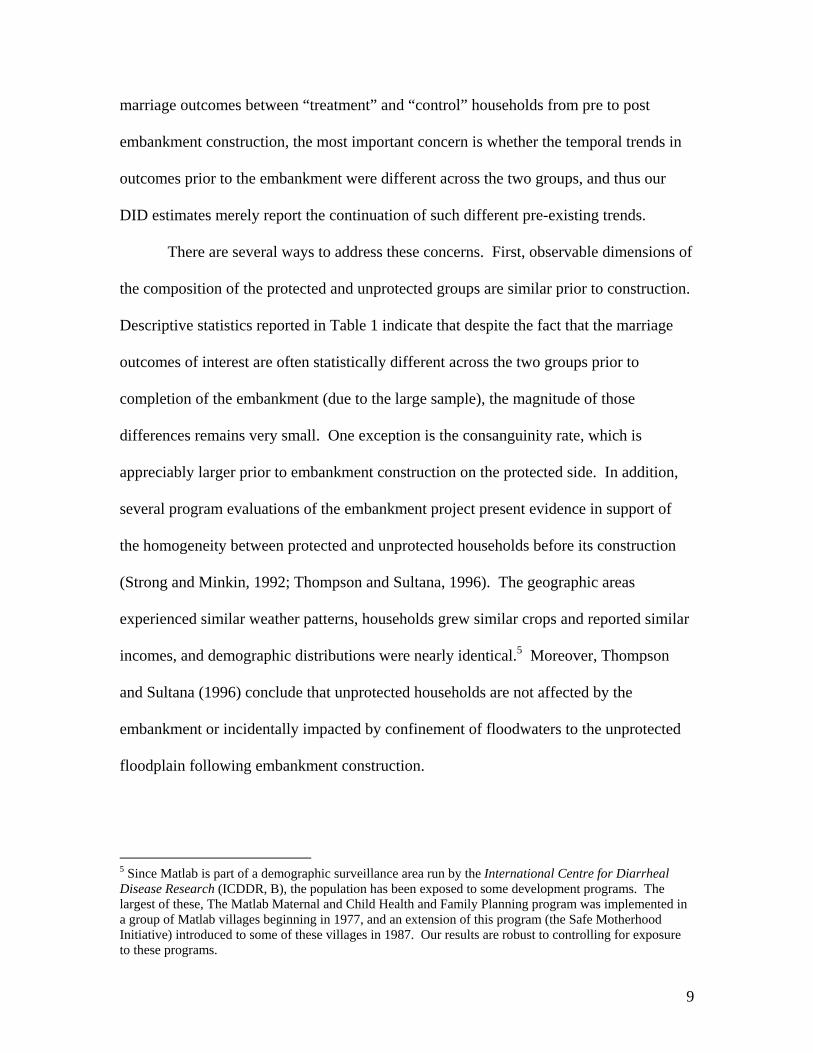
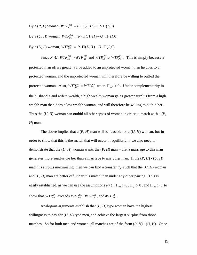
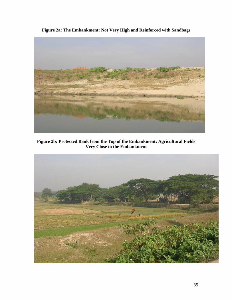
Figure 2a: The Embankment: Not Very High and Reinforced with Sandbags

Figure 2b: Protected Bank from the Top of the Embankment: Agricultural Fields Very Close to the Embankment

36

Figure 3: Land Distribution of Spouses of Protected and Unprotected Men in the Simulated Gale-Shapley Marriage Market

37

Figure 4: Age Distribution of Spouses for Protected Men and Women in the Simulated Gale-Shapley Marriage Market

38

Figure 5: Nash Bargaining Surplus for Men and Women Pre and Post Embankment

39

Figure 6: Assortative Matching in Protection Status in the Simulated Model

Low Search Friction in Marriage Market: qb = 0.90 (probability of seeing a partner on the same bank) qs = 0.50 (probability of seeing a partner on the opposite bank)

Before Embankment After Embankment Same Side of River

Matches 64% 30%

Across the River Matches

36% 70%

With Greater Search Friction in Marriages Across the River: qb = 0.95 qs = 0.30

Before Embankment After Embankment Same Side of River

Matches 78% 42%

Across the River Matches

22% 56%

Even Greater Search Friction in Marriages Across the River: qb = 0.95 qs = 0.20

Before Embankment After Embankment Same Side of River

Matches 83% 48%

Across the River Matches

17% 52%

40

Table 1: Descriptive Statistics Full Sample (ICDDR Matlab Demographic Surveillance Area) Before Embankment After Embankment Mean: protected unprotected protected unprotectedPercentage of Consanguineous Marriages .081** .067** .044*** .059*** (.01) (.00) (.00) (.00) Female Age at Marriage 19.02 19.04 19.90 19.84 (.06) (.05) (.06) (.04) Male Age at Marriage 26.93 25.71 27.33*** 25.96*** (.15) (.10) (.12) (.08) Household Land Owned (1982) 11.12*** 10.28*** 11.44*** 10.64*** (.23) (.15) (.19) (.13) Land Owned by Spouse's Household (1982) 10.82** 9.89** 11.13*** 10.22*** (.31) (.31) (.27) (.20) Percentage of Marriages to Spouse from outside Matlab .478*** .576*** .512*** .597*** (.01) (.00) (.01) (.00) Percentage of Marriages to Spouse from outside Village .864*** .880*** .882*** .895*** (.00) (.00) (.00) (.00) Total Marriage Observations 5225 11050 8438 17896 Standard errors in parentheses. *** indicates t-test significant at 1%, **indicates significant at 5% level. Pre indicates 1985-1986 for consanguinity and 1982-1986 for all other variables. Post indicates 1989-1996. MHSS 1996 Sample

Pre Post Mean: protected unprotected protected unprotectedPercentage of Men Receiving Dowry .11 .12 .42 .43 (.01) (.01) (.04) (.02) Value of Dowry Received by Men 576.08 575.27 4077.90 4193.57 (83.88) (46.82) (487.01) (378.62) Value of Dowry Received by Men in 389.47 524.73 5708.33* 3658.67* Consanguineous Marriages (113.34) (109.60) (1310.88) (561.12) Total Marriage Observations 1119 2543 182 422

Standard errors in parentheses. * indicates t-test significant at 10% level. Pre indicates 1982-1986; Post indicates 1989-1996. Data taken from 1996 MHSS.

41

Table 2: No Pre-existing Differences in Trends in Marriage Outcomes by Protection Status

Consanguineous

Marriage? Spouse Owns Above Average

Amount of Land? Coeff. ME Coeff. ME Protected -2.553 -2.566 (8.164) -.254 (2.223) -.654

Year -.280*** .001 (.056) -.037 (.016) .000

Protected * Year .031 .031 (.096) .004 (.026) .011

Land Owned -.002 (.002) -.000 Above Avg. Amount of Land .144*** (.035) .052

R-squared .011 .003 Total obs. 7130 6199 Sample Pre-Embankment Years (1982-1986) only

Standard errors in parentheses. *** indicates t-test significant at 1% level. All models estimated using probit. All specifications include pre-embankment years 1982-1986 only. Marginal effects calculated at means of explanatory variables.

Table 3: Falsification Tests: Placing the Embankment in a Wrong Location and Wrong Year

Consanguinity Wealthy Spouse?

Falsification Type: Time Location Time Location Percentage of specifications where: T-statistic for actual embankment greater than t-statistic for false embankment 100% 100% 91% 100%

R-sq for actual embankment greater than R-sq for false embankment 88% 50% 100% 50%

Actual embankment coefficient is significant (5%) when included with false embankment 100% 100% 36% 100%

False embankment coefficient is significant (5%) when included with actual embankment 0% 100% 0% 0%

All models estimated using probit. These tests are based on Aghion, Burgess, Redding and Zilibotti (2005). In the difference-in-difference regression specifications, we add a false embankment interaction year (any year in the sample other than 1987) or location alongside the actual embankment interaction term, and repeat the test for all possible years in the data. The table summarizes how often the actual embankment “trumps” these false embankment in its effects on two marriage market outcomes of interest – consanguinity and marrying into wealthy households (i.e. those who own above average amount of land).

42

Table 4: Standardized Mortality Rates

Cause of Death Diarrheal Respiratory Chronic Total Percentage of specifications where: Diseases

Infections Diseases Diseases

AccidentDeaths

Embankment coefficient is negative 53% 47% 50% 50% 47% 44% Embankment is negative significant (at 5% level) 13% 6% 9% 0% 3% 0% Embankment negative significant for: All 30-35yrs M.30-35yrs F.5-15yrs M.Infants F.45-50yrs F.55-60yrs Embankment is positive significant (at 5% level) 0% 0% 3% 9% 0% 3% Embankment positive significant for: F.Elderly M.60-65yrs M.Elderly All Elderly Number of regressions 32

Mortality rates standardized to 1983 village population shares by sex and age category. Age categories start at 0 for infants, and then increase by 5-year age increments through a top age category including everyone over 70 years. Examples of causes of death: cholera or dysentery (diarrheal), malaria or hepatitis (infections), pneumonia or TB (respiratory), heart disease or cancer (chronic), and drowning or violence (accident). All regressions estimated using OLS and include a control variable for villages participating in the Maternal Child Health and Family Planning Program. Tobit models find similar results on coefficient signs.

Table 5: Value of Land in the MHSS Cross-sectional Sample

Value of Land 3613.68 Protected (2473.56) 6.54 Area under Irrigation (13.27) 858.55 Distance to Market (848.08) -33.49 Travel Time to Market (54.50) -5184.93** Credit Institution in Vill. (2367.64) 5987.06** MCHFP Village (2350.82)

Controls by Crop Type: Area under Cultivation Yes Cost of Cultivation Yes R-squared .007 Total obs. 1869

Value of land in taka per decimal in 1996. Data taken from 1996 MHSS, observations are individual landowners. Crop types include: vegetables, aman paddy, aus paddy, aoro paddy, jute, wheat, mustard, potato, dal, and onion. Distance and time to market are calculated from village land is located in; market is defined as either large or small market.

43

Table 6: First-Order Effect of the Endowment on Wealth Asset Indices Pre-embankment Post-embankment Difference Protected Unprotected Protected Unprotected Protected Unprotected

-.05*** .05*** .38 .38 .43*** .34*** (.02) (.01) (.02) (.02) (.02) (.02)

Farmers (Landowners)

Obs. 3377 7270 3377 7270 3377 7270 -.48 -.44 .03*** -.21*** .50*** .23*** (.03) (.02) (.04) (.03) (.05) (.03)

Farmers (Tenant)

Obs. 552 1179 552 1179 552 1179 .07*** .16*** .33*** .42*** .26 .26 (.03) (.02) (.02) (.02) (.03) (.02)

Non-Farm Occupations

Obs. 1530 3207 1530 3207 1530 3207 -.06*** .03*** .33 .33 .39*** .30*** (.01) (.01) (.01) (.01) (.02) (.01)

All Occupations

Obs. 5459 11656 5459 11656 5459 11656 Standard errors in parentheses. *** indicates t-test significant at 1% level; ** indicates significance at 5% level. Asset index constructed using principal components factor analysis, and measures household ownership of any combination of the following assets: radio, watch or clock, bicycle, cows, and hurricane lamp. Data taken from Matlab DSS 1982 and 1996 household censuses.

44

Table 7: Changes in the Variance in Assets across Households within Village Following Embankment Construction

Within-Village Variance in Assets Pre-embankment Post-embankment Protected .87 .91 (.04) (.04) Obs. 32 Unprotected 1.02 .96 (.04) (.02) Obs. 93

Each observation is a village in Matlab, and the table reports the variance in assets across households within a village. Only villages with >80% of land on one side of the embankment or the other are included.

Table 8: Location of Spouse does not Change Differentially after Embankment

Marrying Across the River

Spouse from

Outside Matlab

Spouse from Different Village Northern Villages Southern Villages

Coeff. ME Coeff. ME Coeff. ME Coeff. ME Protected -.247*** -.075*** 1.06*** 1.28*** (.021)

-.098 (.027)

-.015 (.051)

.381 (.046)

.470

Post .053*** .082*** .009 -.040 (.015)

.021 (.020)

.016 (.041)

.003 (.040)

-.015

Embankment .031 .002 .012 .028 (.027)

.012 (.034)

.000 (.066)

.004 (.060)

.011

R-squared .006 .002 .116 .175 No. of obs. 42609 42596 7662 8596

Table 9: …but Unprotected Households More Likely to Marry into Different Occupations

Marrying into Different Occupation

- Full Sample Marrying into Different Occupation -

by Farmers/Non-Farmers

Diff-in-Diff Household

FE Farmers Non-Farmers Coeff. ME Coeff. Coeff. ME Coeff. ME

-.150*** .131 .187*** Protected (.041)

.051 (.080)

.006 (.052)

.074

.019 .014 .067 .078 Post (.031)

-.001 (.026) (.064)

.003 (.040)

.031

.124** -.056 .06 -.128* Embankment (.053)

-.044 (.037) (.100)

.001 (.067)

-.051

R-squared .080 .003 .016 .001 Total obs. 12338 3112 5983 6355

Standard errors in parentheses. *** indicates significance at 1% level. All models estimated using probit. Marginal effects calculated at means of explanatory variables.

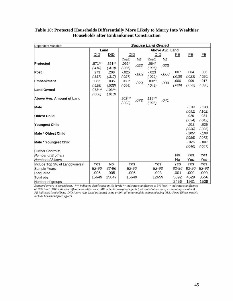
45

Table 10: Protected Households Differentially More Likely to Marry Into Wealthier Households after Embankment Construction

Dependent Variable: Spouse Land Owned Land Above Avg. Land DID DID DID DID FE FE FE Coeff. ME Coeff. ME Protected .871** .851** .062* .064* (.410) (.410) (.035)

.022(.035)

.023 Post .273 .208 -.025 -.023 .007 .004 .006 (.317) (.317) (.027)

-.009(.029)

-.008 (.018) (.023) (.026) Embankment .082 .035 .080* .108** .006 .009 .017 (.528) (.528) (.044)

.029(.048)

.039 (.028) (.032) (.036) Land Owned .073*** .103*** (.008) (.013) Above Avg. Amount of Land .202*** .115*** (.022)

.073(.025)

.041 Male -.109 -.133 (.091) (.102) Oldest Child .020 .034 (.034) (.042) Youngest Child -.013 -.025 (.030) (.035) Male * Oldest Child -.105* -.108 (.056) (.073) Male * Youngest Child -.026 -.007 (.040) (.047) Further Controls: Number of Brothers No Yes Yes Number of Sisters No Yes Yes Include Top 5% of Landowners? Yes No Yes Yes Yes Yes Yes Sample Years 82-96 82-96 82-96 82-93 82-96 82-96 82-93R-squared .006 .005 .006 .003 .001 .000 .000 Total obs. 15649 15047 15649 12659 5892 4529 3556 Number of groups 2456 1931 1538 Standard errors in parentheses. *** indicates significance at 1% level; ** indicates significance at 5% level; * indicates significance at 10% level. DID indicates difference-in-difference; ME indicates marginal effects (calculated at means of explanatory variables); FE indicates fixed effects. DID Above Avg. Land estimated using probit; all other models estimated using OLS. Fixed Effects models include household fixed effects.

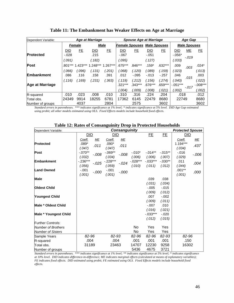
46

Table 11: The Embankment has Weaker Effects on Age at Marriage

Dependent Variable: Age at Marriage Spouse Age at Marriage Age Gap Female Male Female Spouses Male Spouses Male Spouses DID FE DID FE DID FE DID FE DID ME FE Protected -.028 .215 -.067 -.051 -.056* (.091) (.182) (.095) (.127) (.033)

-.019

Post .801*** 1.423*** 1.248*** 1.267*** .675*** .846*** .159* .632*** .009 .024* (.066) (.096) (.131) (.201) (.068) (.120) (.089) (.159) (.023)

.003(.013)

Embankment .086 .116 .158 .391 .012 -.095 -.013 -.257 .046 .003 (.116) (.169) (.231) (.363) (.119) (.212) (.156) (.274) (.040)

.015(.022)

Age at Marriage .321*** .343*** .676*** .659*** -.051*** -.008*** (.004) (.009) (.008) (.021) (.002)

-.017(.002)

R-squared .010 .023 .008 .010 .310 .316 .224 .204 .018 .012 Total obs. 24349 9914 18255 6781 17362 6145 22479 8680 22749 8680 Number of groups 4037 2804 2575 3602 3602

Standard errors in parentheses. *** indicates significance at 1% level; * indicates significance at 5% level. DID Age Gap estimated using probit; all other models estimated using OLS. Fixed Effects models include household fixed effects.

Table 12: Rates of Consanguinity Drop in Protected Households

Dependent Variable: Consanguinity Protected Spouse DID DID FE FE DID Coeff. ME Coeff. ME Coeff. ME Protected .089* .090* 1.194*** (.047)

.011(.047)

.011 (.034) .437

Post -.070** -.069** -.010* -.014** -.015** -.016 (.032)

-.008(.034)

-.008(.006) (.006) (.007) (.029)

-.006

Embankment -.236*** -.228*** -.028*** -.033*** -.030** .011 (.056)

-.025(.059)

-.024(.010) (.011) (.012) (.044)

.004

Land Owned -.001 -.001 .001** (.001)

-.000(.001)

-.000 (.001) .000

Male .039 .038 (.031) (.034) Oldest Child -.005 -.015 (.009) (.012) Youngest Child .007 -.002 (.009) (.011) Male * Oldest Child -.007 .010 (.016) (.021) Male * Youngest Child -.033*** -.020 (.012) (.015) Further Controls: Number of Brothers No Yes Yes Number of Sisters No Yes Yes Sample Years 82-96 82-93 82-96 82-96 82-93 82-96 R-squared .004 .004 .001 .001 .001 .150 Total obs. 31189 23463 14707 12230 9258 16302 Number of groups 5436 4675 3721 Standard errors in parentheses. *** indicates significance at 1% level; ** indicates significance at 5% level; * indicates significance at 10% level. DID indicates difference-in-difference; ME indicates marginal effects (calculated at means of explanatory variables); FE indicates fixed effects. DID estimated using probit; FE estimated using OLS. Fixed Effects models include household fixed effects.

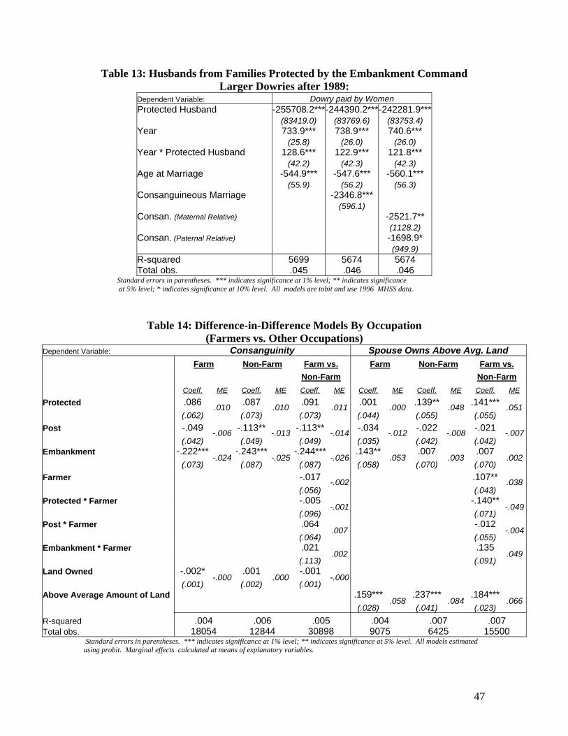
47

Table 13: Husbands from Families Protected by the Embankment Command Larger Dowries after 1989:

Dependent Variable: Dowry paid by Women Protected Husband -255708.2***-244390.2***-242281.9*** (83419.0) (83769.6) (83753.4) Year 733.9*** 738.9*** 740.6*** (25.8) (26.0) (26.0) Year * Protected Husband 128.6*** 122.9*** 121.8*** (42.2) (42.3) (42.3) Age at Marriage -544.9*** -547.6*** -560.1*** (55.9) (56.2) (56.3) Consanguineous Marriage -2346.8*** (596.1) Consan. (Maternal Relative) -2521.7** (1128.2) Consan. (Paternal Relative) -1698.9* (949.9) R-squared 5699 5674 5674 Total obs. .045 .046 .046

Standard errors in parentheses. *** indicates significance at 1% level; ** indicates significance at 5% level; * indicates significance at 10% level. All models are tobit and use 1996 MHSS data.

Table 14: Difference-in-Difference Models By Occupation (Farmers vs. Other Occupations)

Dependent Variable: Consanguinity Spouse Owns Above Avg. Land Farm Non-Farm Farm vs. Farm Non-Farm Farm vs. Non-Farm Non-Farm Coeff. ME Coeff. ME Coeff. ME Coeff. ME Coeff. ME Coeff. ME

Protected .086 .087 .091 .001 .139** .141*** (.062)

.010(.073)

.010(.073)

.011(.044)

.000 (.055)

.048(.055)

.051

Post -.049 -.113** -.113** -.034 -.022 -.021 (.042)

-.006(.049)

-.013(.049)

-.014(.035)

-.012 (.042)

-.008(.042)

-.007

Embankment -.222*** -.243*** -.244*** .143** .007 .007 (.073)

-.024(.087)

-.025(.087)

-.026(.058)

.053 (.070)

.003(.070)

.002

Farmer -.017 .107** (.056)

-.002 (.043)

.038

Protected * Farmer -.005 -.140** (.096)

-.001 (.071)

-.049

Post * Farmer .064 -.012 (.064)

.007 (.055)

-.004

Embankment * Farmer .021 .135 (.113)

.002 (.091)

.049

Land Owned -.002* .001 -.001 (.001)

-.000(.002)

.000(.001)

-.000

Above Average Amount of Land .159*** .237*** .184*** (.028)

.058 (.041)

.084(.023)

.066

R-squared .004 .006 .005 .004 .007 .007 Total obs. 18054 12844 30898 9075 6425 15500

Standard errors in parentheses. *** indicates significance at 1% level; ** indicates significance at 5% level. All models estimated using probit. Marginal effects calculated at means of explanatory variables.

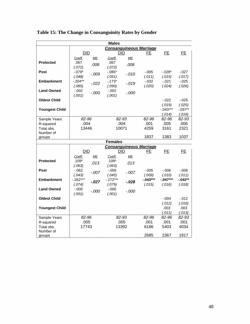
48

Table 15: The Change in Consanguinity Rates by Gender

Males Consanguineous Marriage DID DID FE FE FE Coeff. ME Coeff. ME Protected .067 .067 (.072)

.008 (.072)

.008 Post -.079* -.085* -.005 -.028* -.027 (.048) -.009 (.051) -.010 (.011) (.015) (.017) Embankment -.204** -.173* -.032 -.021 -.025 (.085) -.022 (.090) -.019 (.020) (.024) (.026) Land Owned -.002 -.002 (.001)

-.000 (.001)

-.000 Oldest Child -.022 -.025 (.019) (.025) Youngest Child -.043*** -.037** (.014) (.016) Sample Years 82-96 82-93 82-96 82-96 82-93 R-squared .004 .004 .001 .005 .006 Total obs. 13446 10071 4259 3161 2321 Number of groups 1837 1383 1037

Females Consanguineous Marriage DID DID FE FE FE Coeff. ME Coeff. ME Protected .109* .109* (.063)

.013 (.063)

.013 Post -.062 -.056 -.005 -.006 -.006 (.043) -.007 (.045) -.007 (.009) (.010) (.011) Embankment -.262*** -.272*** -.043*** -.047*** -.042** (.074) -.027 (.079) -.028 (.015) (.016) (.018) Land Owned -.000 -.000 (.001)

-.000 (.001)

-.000 Oldest Child -.004 -.012 (.012) (.016) Youngest Child .003 .003 (.011) (.013) Sample Years 82-96 82-93 82-96 82-96 82-93 R-squared .005 .005 .001 .001 .001 Total obs. 17743 13392 6186 5403 4034 Number of groups 2685 2367 1817

49

References Aghion, P., Burgess, R., Redding, Stephen, and F. Zilibotti. 2005. “The Unequal Effects

of Liberalization: Evidence from Dismantling the License Raj in India,” NBER Working Paper 12031.

Anderson, Siwan 2000. “The Economics of Dowry Payments in Pakistan,” mimeo, Tilburg University

Anderson, Siwan 2005. “Why the Marriage Squeeze Cannot Cause Dowry Inflation,” Journal of Economic Theory, in press.

Becker G. (1991). Treatise on the Family, Harvard University Press, Cambridge, MA Bergstrom, Theodore (1997). “A Survey of Theories of the Family,” 21-74 in M.

Rosenzweig and O. Stark eds, Handbook of Population and Family Economics: Amsterdam, Elsevier Science.

Bertrand, M., Duflo, E. and S. Mullainathan. 2004. “How Much Should We Trust Differences-In-Differences Estimates?” Quarterly Journal of Economics 119 (1): 249-275.

Bittles, A.H. 2001. “Consanguinity and its Relevance to Clinical Genetics,” Clinical Genetics 60: 89-98.

Bittles, A.H. 1994. “The Role and Significance of Consanguinity as a Demographic Variable,” Population and Development Review 20(3): 561-584.

Bittles, A.H. and J.V. Neel. 1994. “The Costs of Human Inbreeding and their Implications for Variations at the DNA Level,” Nature Genetics 8: 117-121.

Bittles, A.H. Mason, W.M., Greene, J., and N. Appaji Rao. 1991. “Reproductive Behavior and Health in Consanguineous Marriages,” Science 252: 789-794.

Bittles, A.H. and U. Makov. 1988. “Inbreeding in Human Populations: Assessment of the Costs,” in Mating Patterns, C. Mascie-Taylor and A. Boyce (ed.), Cambridge: Cambridge University Press.

Bloch, F., Rao, V. and S. Desai. 2004. “Wedding Celebrations as Conspicuous Consumption: Signaling Social Status in Rural India,” Journal of Human Resources 39(3): 675-695.

Bloch, F. and V. Rao. 2002. “Terror as a Bargaining Instrument: A Case-Study of Dowry Violence in Rural India,” American Economic Review 92(4): 1029-1043.

Briscoe, J. 1998. “Against the Flow: Reflections on Two Decades of Development in a Bangladeshi Village,” unpublished paper

Browning, M., Chiappori, P.A., and Weiss, Y. 2003. “A Simple Matching Model of the Marriage Market,” mimeo, University of Chicago.

Browning, M., Chiappori, P. and Y.Weiss (2005). Family Economics, Cambridge University Press, Cambridge, UK, forthcoming.

Caldwell, J., Reddy, P., and P. Caldwell. 1983. “Causes of Marriage Change in South India,” Population Studies 37(3): 343-361.

Dalmia, S. 2004. “A Hedonic Analysis of Marriage Transactions in India: Estimating Determinants of Dowries and Demand for Groom Characteristics in Marriage,” Research in Economics 58: 235-255.

Dalmia, S. and P. Lawrence. 2001. “An Empirical Analysis of Assortative Mating in India and the U.S.,” International Advances in Economic Research 7(4): 443-458.

Deolalikar, A. and V. Rao. 1998. “The Demand for Dowries and Bride Characteristics in

50

Marriage: Empirical Estimates for Rural South-Central India,” in Gender, Population, and Development, M. Krishnaraj, R. Sudarshan, A. Sharif (ed.), Oxford University Press.

Dyson, T. and M. Moore. 1983. “On Kinship Structure, Female Autonomy, and Demographic Behavior in India,” Population and Development Review 9(1): 35-60.

Field, E. and Ambrus, A. 2005. “Early Marriage and Female Schooling in Bangladesh,” Working Paper

Fruzzetti, L. 1982. The Gift of a Virgin: Women, Marriage and Ritual in a Bengali Society, Rutgers University Press.

Grossbard-Schechtman, A. 1984. “A Theory of Allocation of Time in Markets for Labor and Marriage,” Economic Journal 94: 863-882.

Haque, C. and M. Zaman. 1993. “Human Responses to Riverine Hazards in Bangladesh: A Proposal for Sustainable Floodplain Development,” World Development 21(1): 93-107.

Hashmi, M. 1997. “Frequency of Consanguinity and its Effect on Congenital Malformation—A Hospital Based Study,” Journal of the Pakistan Medical Association 47: 75-78.

Huq, L. and S. Amin. 2001. “Dowry Negotiations and the Process of Union Formation in Bangladesh: The Implications of Rising Education.” Paper presented at the Annual Meetings of the Population Association of America.

Hurt, L., Ronsmans, C., Campbell, O., Saha, S., Kenward, M. and M. Quigley. 2004. “Long-Term Effects of Reproductive History on All-Cause Mortality Among Adults in Rural Bangladesh,” Studies in Family Planning 35(3): 189-196.

Hussain, R., and Bittles, A.H. 1999. “Differentials in Age at Marriage, Contraceptive Use and Fertility in Consanguineous Marriages in Pakistan,” Journal of Biosocial Science 31: 121-138.

Jahan, R. 1991. “Hidden Wounds, Visible Scars: Violence Against Women in Bangladesh,” in Structures of Patriarchy: State, Community and Household in Modernising Asia, B. Agarwal (ed.), Kali for Women, New Delhi.

Jensen, R., and R. Thornton. 2003. “Early Female Marriage in the Developing World,” Gender and Development 11(2): 9-19.

Kabir, M. 2004. “Development or a Disaster Forgotten? The Case of Meghna- Dhonogoda Irrigation and Flood Control Project.”

Khan, Nizam Myaux, J.A., Ali, M., Chakraborty, J., and A. de Francisco. 1997. “Flood Control

Embankments Contribute to the Improvement of the Health Status of Children in Rural Bangladesh,” Bulletin of the World Health Organization 75(6): 533-539.

Paul, B. 1995. “Farmers’ Responses to the Flood Action Plan (FAP) of Bangladesh: An Empirical Study,” World Development 23(2): 299-309.

Rao, V., 1993. “The Rising Price of Husbands: A Hedonic Analysis of Dowry Increases in Rural India,” Journal of Political Economy 101: 666-677.

Rosenzweig, M. and O. Stark. 1989. “Consumption-Smoothing, Migration, and Marriage: Evidence from Rural India,” Journal of Political Economy 97: 905-926.

Shah, G., Toney, M., and B. Pitcher. 1998. “Consanguinity and Child Mortality: The

51

Risk Faced by Families,” Population Research and Policy Review 17: 275-283. Siow, Aloysius, 1998. “Differential Fecundity, Markets and Gender Roles,” Journal of

Political Economy 106 (2): 334-354. Strong, M. and S. Minkin. 1992. “The Demographic, Health, and Nutritional Impacts of

the Meghna-Dhonagoda Embankment,” Bangladesh Flood Action Plan FAP 16 Environmental Study, Special Studies Program. ICDDR,B and ISPAN.

Thompson, P.M. and P. Sultana. 1996. “Distributional and Social Impacts of Flood Control in Bangladesh,” The Geographical Journal 162(1): 1-13.

Tiemoko, R. 2001. “The Gender Age Gap: Marriage and Rights in the Cote d’Ivoire,” Development 44(2): 104-106.

Weiss, Yoram (1997). “The Formation and Dissolution of Families: Why Marry? Who Marries Whom? And What Happens Upon Divorce,” 81-124 in M. Rosenzweig and O. Stark eds, Handbook of Population and Family Economics: Amsterdam, Elsevier Science.

Wickrama, K. and F. Lorenz. 2002. “Women’s Status, Fertility Decline, and Women’s Health in Developing Countries: Direct and Indirect Influences of Social Status on Health,” Rural Sociology 67(2): 255-277.

52

Appendix

Table A1: List of Variables Marriage Outcome Definition Value of Dowry Total estimated cash value of dowry paid to husband in Taka Consanguinity Individual married 1st, 2nd, or other cousin Spouse Land Owned Land owned by head of spouse’s household in 1982

(measured in decimals) Spouse Above Average Land Spouse’s household owns more than 10.347 decimals of land

(avg. land owned by households of spouses chosen within the sample period)

Age at Marriage Age of individual at time of marriage Spouse Age at Marriage Age of spouse at time of marriage Spouse Age Gap Indicator for whether or not male spouse is more than 10 years

older than the female marriage observation Protected Spouse Group status of spouse (time-invariant indicator for whether or

not spouse’s household is protected by embankment) Explanatory Variables Definition Protected Group status of individual Post Indicator equal to 1 if marriage year between 1989-1996 and 0 if

marriage year between 1982-1987 Embankment Embankment effect (interaction of Protected and Post) Land Owned Land owned by head of individual’s household in 1982 Above Average Land Owned Household owns more than 10.744 decimals of land (avg. land

owned by households of individuals getting married within the sample period)

Farmer Indicator equal to 1 if household head is a farmer and 0 otherwise

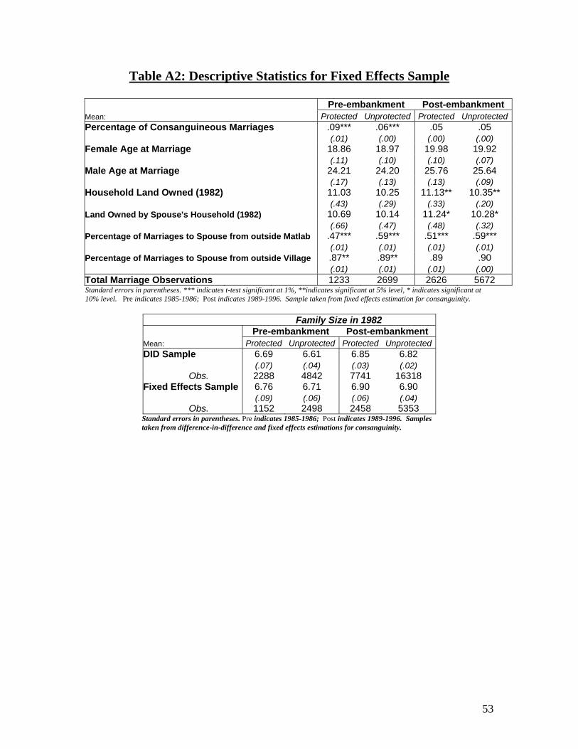
53

Table A2: Descriptive Statistics for Fixed Effects Sample

Pre-embankment Post-embankment Mean: Protected Unprotected Protected UnprotectedPercentage of Consanguineous Marriages .09*** .06*** .05 .05 (.01) (.00) (.00) (.00) Female Age at Marriage 18.86 18.97 19.98 19.92 (.11) (.10) (.10) (.07) Male Age at Marriage 24.21 24.20 25.76 25.64 (.17) (.13) (.13) (.09) Household Land Owned (1982) 11.03 10.25 11.13** 10.35** (.43) (.29) (.33) (.20) Land Owned by Spouse's Household (1982) 10.69 10.14 11.24* 10.28* (.66) (.47) (.48) (.32) Percentage of Marriages to Spouse from outside Matlab .47*** .59*** .51*** .59*** (.01) (.01) (.01) (.01) Percentage of Marriages to Spouse from outside Village .87** .89** .89 .90 (.01) (.01) (.01) (.00) Total Marriage Observations 1233 2699 2626 5672 Standard errors in parentheses. *** indicates t-test significant at 1%, **indicates significant at 5% level, * indicates significant at 10% level. Pre indicates 1985-1986; Post indicates 1989-1996. Sample taken from fixed effects estimation for consanguinity.

Family Size in 1982 Pre-embankment Post-embankment Mean: Protected Unprotected Protected Unprotected DID Sample 6.69 6.61 6.85 6.82 (.07) (.04) (.03) (.02) Obs. 2288 4842 7741 16318 Fixed Effects Sample 6.76 6.71 6.90 6.90 (.09) (.06) (.06) (.04) Obs. 1152 2498 2458 5353

Standard errors in parentheses. Pre indicates 1985-1986; Post indicates 1989-1996. Samples taken from difference-in-difference and fixed effects estimations for consanguinity.

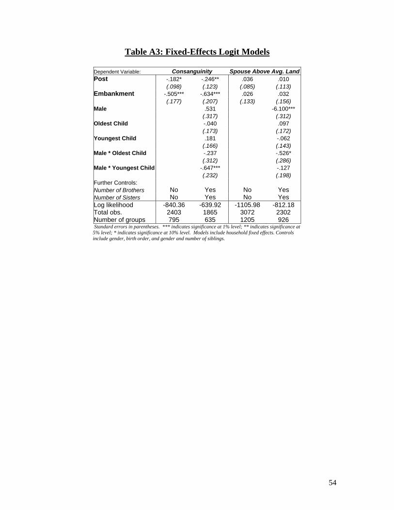
54

Table A3: Fixed-Effects Logit Models

Dependent Variable: Consanguinity Spouse Above Avg. Land Post -.182* -.246** .036 .010 (.098) (.123) (.085) (.113) Embankment -.505*** -.634*** .026 .032 (.177) (.207) (.133) (.156) Male .531 -6.100*** (.317) (.312) Oldest Child -.040 .097 (.173) (.172) Youngest Child .181 -.062 (.166) (.143) Male * Oldest Child -.237 -.526* (.312) (.286) Male * Youngest Child -.647*** -.127 (.232) (.198) Further Controls: Number of Brothers No Yes No Yes Number of Sisters No Yes No Yes Log likelihood -840.36 -639.92 -1105.98 -812.18 Total obs. 2403 1865 3072 2302 Number of groups 795 635 1205 926

Standard errors in parentheses. *** indicates significance at 1% level; ** indicates significance at 5% level; * indicates significance at 10% level. Models include household fixed effects. Controls include gender, birth order, and gender and number of siblings.

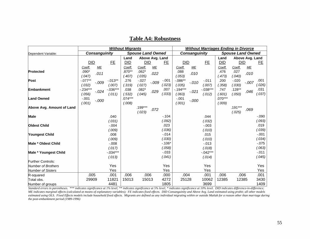
55

Table A4: Robustness

Without Migrants Without Marriages Ending in Divorce Dependent Variable: Consanguinity Spouse Land Owned Consanguinity Spouse Land Owned Land Above Avg. Land Land Above Avg. Land DID FE DID DID FE DID FE DID DID FE Coeff. ME Coeff. Coeff. ME Coeff. ME Coeff. Coeff. ME Protected .090* .870** .062* .088 .476 .027 (.047)

.011 (.407) (.035)

.022 (.053) .010

(.473) (.040) .010

Post -.077** -.013** .276 -.027 -.001 -.086** -.011 .200 -.020 .001 (.032)

-.009(.007) (.319) (.027)

-.009 (.023) (.035) -.010

(.007) (.358) (.030) -.007 (.026)

Embankment -.234*** -.036*** .038 .082* .007 -.194*** -.038*** .747 .128** .031 (.056)

-.024(.011) (.532) (.045)

.029 (.033) (.063) -.021

(.012) (.601) (.050) .046 (.037)

Land Owned -.001 .074*** -.001 .070*** (.001)

-.000 (.008) (.001)

-.000 (.009)

Above Avg. Amount of Land .199*** .191*** (.023)

.072 (.025) .069

Male .040 -.104 .044 -.090

(.031) (.092) (.032) (.093)

Oldest Child -.004 .023 -.003 .019

(.009) (.036) (.010) (.039)

Youngest Child .008 -.014 .015 -.001

(.009) (.030) (.010) (.034)

Male * Oldest Child -.008 -.106* -.013 -.075

(.017) (.058) (.018) (.063)

Male * Youngest Child -.034*** -.033 -.042*** -.011 (.013) (.041) (.014) (.045)Further Controls: Number of Brothers Yes Yes Yes Yes Number of Sisters Yes Yes Yes Yes R-squared .005 .001 .006 .006 .000 .004 .001 .006 .006 .001Total obs. 29909 11821 15013 15013 4272 25128 10062 12385 12385 3430Number of groups 4481 1805 3699 1409Standard errors in parentheses. *** indicates significance at 1% level; ** indicates significance at 5% level; * indicates significance at 10% level. DID indicates difference-in-difference; ME indicates marginal effects (calculated at means of explanatory variables); FE indicates fixed effects. DID Consanguinity and Above Avg. Land estimated using probit; all other models estimated using OLS. Fixed Effects models include household fixed effects. Migrants are defined as any individual migrating within or outside Matlab for a reason other than marriage during the post-embankment period (1989-1996)