Markus K. Brunnermeier LECTURE 08: MULTI-PERIOD MODEL ... · FIN501 Asset Pricing Lecture 08 Option Pricing (1) LECTURE 08: MULTI-PERIOD MODEL OPTIONS: BLACK-SCHOLES-MERTON Markus

FIN501 Asset PricingLecture 08 Option Pricing (1)

LECTURE 08: MULTI-PERIOD MODELOPTIONS: BLACK-SCHOLES-MERTON

Markus K. Brunnermeier


specifyPreferences &

Technology

observe/specifyexisting

Asset Prices

State Prices q(or stochastic discount

factor/Martingale measure)

derivePrice for (new) asset

• evolution of states• risk preferences• aggregation

absolute asset pricing

relativeasset pricing

NAC/LOOP

LOOP

NAC/LOOP

Only works as long as market completeness doesn’t change

deriveAsset Prices


• Price claim at 𝑡 = 0 with many final payoffs at 𝑇

o 𝑆 states/histories

• Dynamic replication with only 2 assets

o Dynamic trading strategy


Option Pricing

• European call option maturing at time 𝑇 with strike 𝐾 ⇒𝐶𝑇 = 𝑆𝑇 − 𝐾

+, no cash flows in between

• Why multi-period problemo Not able to statically replicate this payoff

using just the stock and risk-free bond

o Need to dynamically hedge – required stock position changes for each period until maturity• Recall static hedge for forward, using put-call parity

• Replication strategy depends on specified random process need to know how stock price evolves over time. o Binomial (Cox-Ross-Rubinstein) model is canonical


Binominal Option Pricing

• Assumptions:o Bond:

• Constant risk-free rate 𝑅𝑓 = 𝑅𝑡𝑓∀𝑡

𝑅𝑓 = 𝑒𝑟𝑇/𝑛 for period with length 𝑇 𝑛

o Stock: • which pays no dividend

• stock price moves from 𝑆 to either 𝑢𝑆 or 𝑑𝑆,

• i.i.d. over time ⇒ final distribution of 𝑆𝑇 is binomial

• No arbitrage: 𝑢 > 𝑅𝑓 > 𝑑

𝑢𝑆

𝑑𝑆

𝑆


A One-Period Binomial Tree

• Example of a single-period model

o 𝑆 = 50, 𝑢 = 2, 𝑑 = 0.5, 𝑅𝑓 = 1.25

o What is value of a European call option with 𝐾 = 50?o Option payoff: 𝑆𝑇 − 𝐾

+

o Use replication to price

100

25

50

50

0

𝐶 =?


Single-period Replication

• Long ∆ stocks and 𝐵 dollars in bond• Payoff from portfolio:

• 𝐶𝑢 option payoff in up state and 𝐶𝑑 as option payoff in down state

𝐶𝑢 = 50, 𝐶𝑑 = 0

• Replicating strategy must match payoffs:𝐶𝑢 = Δ𝑢𝑆 + 𝑅

𝑓𝐵𝐶𝑑 = Δ𝑑𝑆 + 𝑅

𝑓𝐵

Δ𝑢𝑆 + 𝑅𝑓𝐵 = 100Δ + 1.25𝐵

Δ𝑑𝑆 + 𝑅𝑓𝐵 = 25Δ + 1.25𝐵

Δ𝑆 + 𝐵 = 50Δ + 𝐵


Single-period Replication

• Solving these equations yields:

Δ =𝐶𝑢 − 𝐶𝑑𝑆 𝑢 − 𝑑

𝐵 =𝑢𝐶𝑑 − 𝑑𝐶𝑢𝑅𝐹 𝑢 − 𝑑

• In previous example, Δ =2

3and 𝐵 = −13.33, so the option value is

𝐶 = Δ𝑆 + 𝐵 = 20

• Interpretation of Δ: sensitivity of call price to a change in the stock price. Equivalently, tells you how to hedge risk of optiono To hedge a long position in call, short Δ shares of stock


Risk-neutral Probabilities

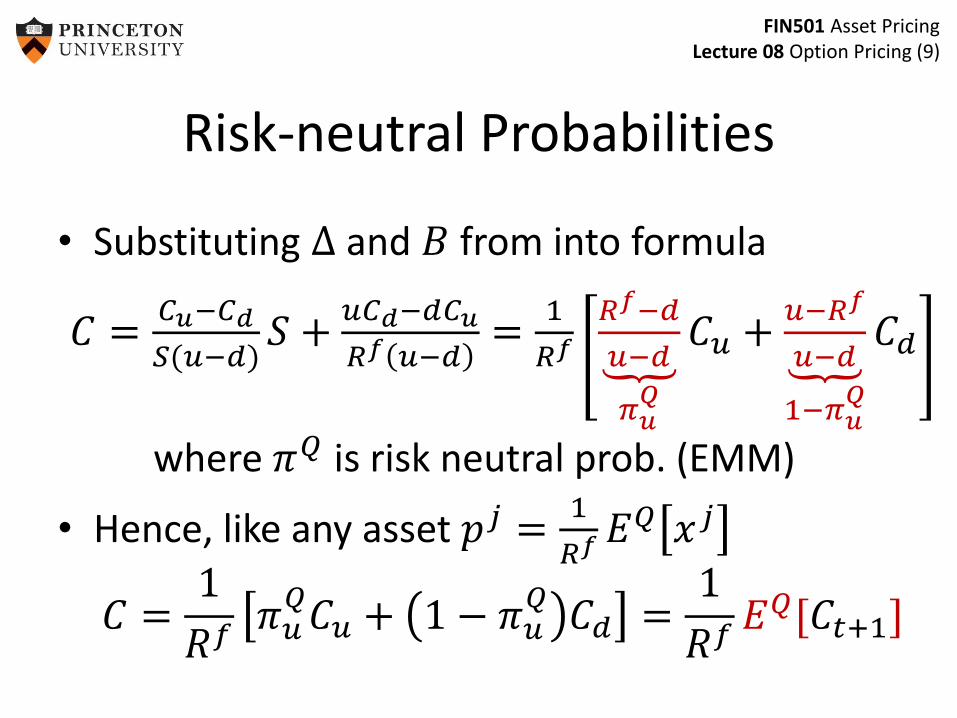
• Substituting Δ and 𝐵 from into formula

𝐶 =𝐶𝑢−𝐶𝑑

𝑆(𝑢−𝑑)𝑆 +𝑢𝐶𝑑−𝑑𝐶𝑢

𝑅𝑓 𝑢−𝑑=1

𝑅𝑓 𝑅𝑓−𝑑

𝑢−𝑑

𝜋𝑢𝑄

𝐶𝑢 + 𝑢−𝑅𝑓

𝑢−𝑑

1−𝜋𝑢𝑄

𝐶𝑑

where 𝜋𝑄 is risk neutral prob. (EMM)

• Hence, like any asset 𝑝𝑗 =1

𝑅𝑓𝐸𝑄 𝑥𝑗

𝐶 =1

𝑅𝑓𝜋𝑢𝑄𝐶𝑢 + 1 − 𝜋𝑢

𝑄𝐶𝑑 =1

𝑅𝑓𝐸𝑄[𝐶𝑡+1]


Risk-neutral Probabilities

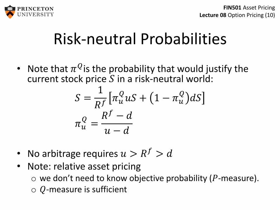
• Note that 𝜋𝑄is the probability that would justify the current stock price 𝑆 in a risk-neutral world:

𝑆 =1

𝑅𝑓𝜋𝑢𝑄𝑢𝑆 + 1 − 𝜋𝑢

𝑄𝑑𝑆

𝜋𝑢𝑄=𝑅𝑓 − 𝑑

𝑢 − 𝑑

• No arbitrage requires 𝑢 > 𝑅𝑓 > 𝑑• Note: relative asset pricing

o we don’t need to know objective probability (𝑃-measure).o 𝑄-measure is sufficient


The Binomial Formula in a Graph


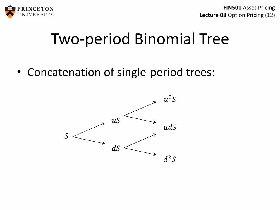
Two-period Binomial Tree

• Concatenation of single-period trees:

𝑢𝑆

𝑑𝑆

𝑆

𝑢2𝑆

𝑢𝑑𝑆

𝑑2𝑆



• Example: 𝑆 = 50, 𝑢 = 2, 𝑑 = 0.5, 𝑅𝑓 = 1.25

• Option payoff:

100

2550

200

50

12.5

𝐶𝑢

𝐶𝑑𝐶

150

0

0



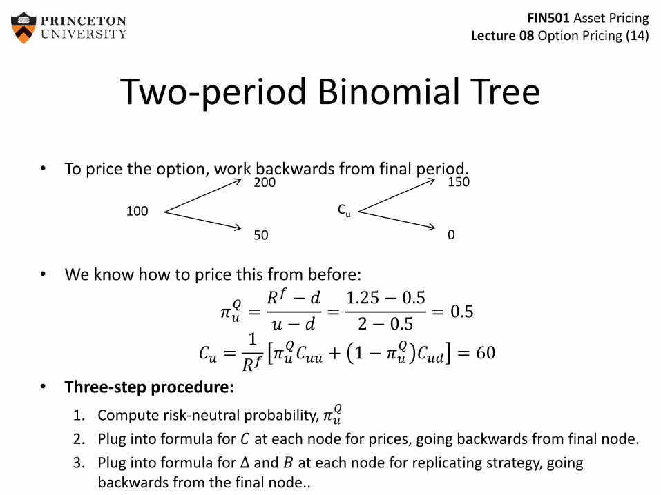
• To price the option, work backwards from final period.

• We know how to price this from before:

𝜋𝑢𝑄=𝑅𝑓 − 𝑑

𝑢 − 𝑑=1.25 − 0.5

2 − 0.5= 0.5

𝐶𝑢 =1

𝑅𝑓𝜋𝑢𝑄𝐶𝑢𝑢 + 1 − 𝜋𝑢

𝑄𝐶𝑢𝑑 = 60

• Three-step procedure:

1. Compute risk-neutral probability, 𝜋𝑢𝑄

2. Plug into formula for 𝐶 at each node for prices, going backwards from final node.

3. Plug into formula for Δ and 𝐵 at each node for replicating strategy, going backwards from the final node..

100

200

50

Cu

150

0



• General formulas for two-period tree:

• 𝜋𝑢𝑄= (𝑅 − 𝑑)/(𝑢 − 𝑑)

• Synthetic option requires dynamic hedgingo Must change the portfolio as stock price moves

𝐶𝑢 =𝜋𝑢𝑄𝐶𝑢𝑢 + 1 − 𝜋𝑢

𝑄 𝐶𝑢𝑑𝑅𝑓

∆𝑢 =𝐶𝑢𝑢 − 𝐶𝑢𝑑

𝑢2𝑆 − 𝑢𝑑𝑆𝐵𝑢 = 𝐶𝑢 − ∆𝑢𝑆

𝐶𝑑 =𝜋𝑢𝑄𝐶𝑢𝑑 + 1 − 𝜋𝑢

𝑄 𝐶𝑑𝑑𝑅𝑓

∆𝑑 =𝐶𝑢𝑑 − 𝐶𝑑𝑑𝑢𝑑𝑆 − 𝑑2𝑆

𝐵𝑑 = 𝐶𝑑 − ∆𝑑𝑆

𝐶 =𝜋𝑢𝑄𝐶𝑢 + 1 − 𝜋𝑢

𝑄 𝐶𝑑𝑅𝑓

=𝜋𝑢𝑄2𝐶𝑢𝑢 + 2𝜋𝑢

𝑄1 − 𝜋𝑢𝑄𝐶𝑢𝑑 + 1 − 𝜋𝑢

𝑄 2𝐶𝑢𝑑

𝑅𝑓 2

Δ =𝐶𝑢 − 𝐶𝑑𝑢𝑆 − 𝑑𝑆

, 𝐵 = 𝐶 − ∆𝑆

𝐶𝑢𝑢

𝐶𝑢𝑑

𝐶𝑑𝑑


Arbitraging a Mispriced Option

• 3-period tree:

o 𝑆 = 80, 𝐾 + 80, 𝑢 = 1.5, 𝑑 = 0.5, 𝑅 = 1.1

• Implies 𝜋𝑢𝑄=𝑅𝑓−𝑑

𝑢−𝑑= 0.6

• Cost of dynamic replication strategy $34.08• If the call is selling for $36, how to arbitrage?

o Sell the real callo Buy the synthetic call

• Up-front profit:

o 𝐶 − ∆𝑆 + 𝐵 = 36–34.08 = 1.92


Towards Black-Scholes• General binomial formula for a European call on non-dividend paying stock 𝑛 periods from expiration:

𝐶 =1

(𝑅𝑓)𝑛

𝑗=0

𝑛𝑛!

𝑗! 𝑛 − 𝑗 !𝜋𝑢𝑄 𝑗1 − 𝜋𝑢𝑄𝑛−𝑗

𝑢𝑗𝑑𝑛−𝑗𝑆 − 𝐾+

• Take parameters:

𝑢 = 𝑒𝜎𝑇𝑛, 𝑑 =1

𝑢= 𝑒−𝜎𝑇𝑛

• Where:o 𝑛 = number of periods in treeo 𝑇 = time to expiration (e.g., measured in years)o 𝜎 = standard deviation of continuously compounded return

o Also take 𝑅𝑓 = 𝑒𝑟𝑓𝑇

𝑛

• As 𝑛 → ∞o Binominal tree → geometric Brownian motiono Binominal formula → Black Scholes Merton


Black-Scholes

𝐶 = 𝑆𝒩 𝑑1 − 𝐾𝑒−𝑟𝑓𝑇𝒩 𝑑2

𝑑1 =1

𝜎 𝑇ln𝑆

𝐾+ 𝑟𝑓 +

𝜎2

2𝑇

𝑑2 =1

𝜎 𝑇ln𝑆

𝐾+ 𝑟𝑓 −

𝜎2

2𝑇 = 𝑑1 − 𝜎 𝑇

o 𝑆 = current stock price o 𝐾 = strikeo 𝑇 = time to maturity o 𝑟 = annualized continuously compounded risk-free rate, o 𝜎 = annualized standard dev. of cont. comp. rate of return on underlying

• Price of a put-option by put-call parity𝑃 = 𝐶 − 𝑆 + 𝐾𝑒−𝑟𝑇

= 𝐾𝑒−𝑟𝑇𝒩 −𝑑2 − 𝑆𝒩 −𝑑1


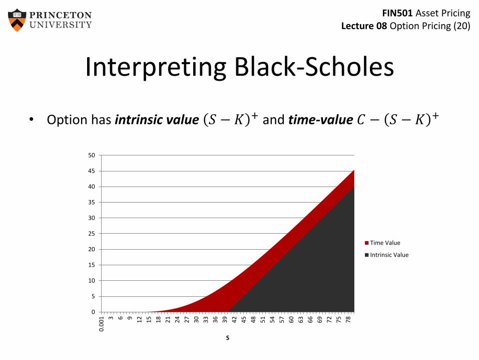
Interpreting Black-Scholes

• Option has intrinsic value 𝑆 − 𝐾 + and time-value 𝐶 − 𝑆 − 𝐾 +

0

5

10

15

20

25

30

35

40

45

50

0.0

01 3 6 9

12

15

18

21

24

27

30

33

36

39

42

45

48

51

54

57

60

63

66

69

72

75

78

S

Time Value

Intrinsic Value


Delta

• Δ is the sensitivity of option price to a small change in the stock priceo Number of shares needed to make a synthetic call

o Also measures riskiness of an option position

Δ𝑐 = 𝒩 𝑑1𝐵𝑐 = −𝐾𝑒

𝑟𝑇𝒩 𝑑2• Delta of

o Call: Δ𝑐 ∈ [0,1] Put: Δ𝑐 ∈ [−1,0]

o Stock: 1 Bond: 0

o portfolio: 𝑗 ℎ𝑗Δ𝑖

NB: For 𝑆 = 𝐾 and 𝑇 → 0, Δ =𝒩 𝑑1 =1

2


Option Greeks

• What happens to option price when one input changes?

o Delta (Δ): change in option price when stock increases by $1

o Gamma (Γ): change in delta when option price increases by $1

o Vega: change in option price when volatility increases by 1%

o Theta (𝜃): change in option price when time to maturity decreases by 1 day

o Rho (𝜌): change in option price when interest rate rises by 1%

• Greek measures for portfolios

o The Greek measure of a portfolio is weighted average of Greeks of individual portfolio components:


Delta-Hedging

• Portfolio ℎ is delta-neutral if 𝑗 ℎ𝑗Δ𝑗 = 0

• Delta-neutral portfolios are a way to hedge out the risk of an option (or portfolio of options)o Example: suppose you write 1 European call whose delta is 0.61.

How can you trade to be delta-neutral?

ℎ𝑐Δ𝑐 + ℎ𝑠Δ𝑠 = −1 0.61 + ℎ𝑠 1 = 0

o So we need to hold 0.61 shares of the stock.

• Delta hedging makes you directionally neutral on the position.o But only linearly! - Γ


Portfolio Insurance & 1987 Crash

• Δ-replication strategy leads to inverse demand

o Sell when price goes down

o Buy when price goes up

• ⇒ Destabilizes market

• 1987 – (uninformed) portfolio insurance trading was interpreted as “informed” sellers.


Notes on Black-Scholes

• Delta-hedging is not a perfect hedge if you do not trade continuouslyo Delta-hedging is a linear approximation to the option valueo But convexity implies second-order derivatives mattero Hedge is more effective for smaller price changes

• Delta-Gamma hedging reduces the basis risk of the hedge.• B-S model assumes that volatility is constant over time and

returns are normal – no fat tails. o Volatility “smile”o BS underprices out-of-the-money puts (and thus in-the-money calls)o BS overprices out-of-the-money calls (and thus in-the-money puts)o Ways forward: stochastic volatility

• Other issues: stochastic interest rates, bid-ask transaction costs, etc.


Implied Vol., Smiles and Smirks

• Implied volatilityo Use current option price and assume B-S model

holds

o Back out volatility

o VIX versus implied volatility of 500 stocks

• Smile/Smirko Implied volatility across various strike prices

• BS implies horizontal line

o Smile/Smirk after 1987 Smile/smirk

K

s2


Merton Model

• Firm’s balance sheet

o Call on equity is essential a “call on a call”

• Merton: Observe equity prices (including vol) and back out o firm value

o debt value

A L

AssetsFollowGeometricBrownian M.

Debt

Equity Call option payoff (long)

Put option payoff (short)


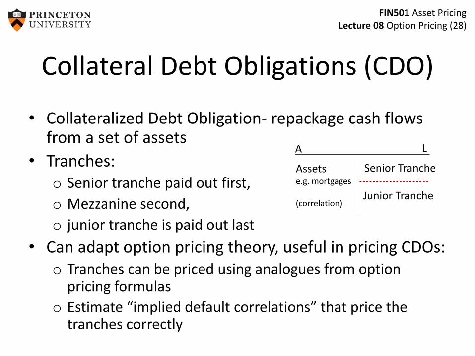
Collateral Debt Obligations (CDO)

• Collateralized Debt Obligation- repackage cash flows from a set of assets

• Tranches: o Senior tranche paid out first,

o Mezzanine second,

o junior tranche is paid out last

• Can adapt option pricing theory, useful in pricing CDOs:o Tranches can be priced using analogues from option

pricing formulas

o Estimate “implied default correlations” that price the tranches correctly

A L

Assetse.g. mortgages

(correlation)

Senior Tranche

Junior Tranche


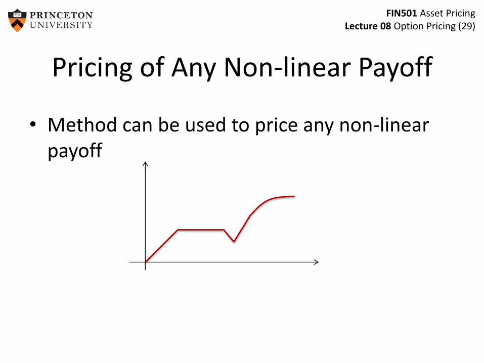
Pricing of Any Non-linear Payoff

• Method can be used to price any non-linear payoff

Documents

Markus K. Brunnermeier LECTURE 08: MULTI-PERIOD MODEL ... · FIN501 Asset Pricing Lecture 08 Option Pricing (1) LECTURE 08: MULTI-PERIOD MODEL OPTIONS: BLACK-SCHOLES-MERTON Markus