Embed Size (px)
Citation preview
Markovian Score Climbing: Variational Inferencewith KL(p||q)
Christian A. NaessethColumbia University, USA
Fredrik LindstenLinköping University, Sweden
David BleiColumbia University, [email protected]
Abstract
Modern variational inference (VI) uses stochastic gradients to avoid intractableexpectations, enabling large-scale probabilistic inference in complex models.VI posits a family of approximating distributions q and then finds the mem-ber of that family that is closest to the exact posterior p. Traditionally, VIalgorithms minimize the “exclusive Kullback-Leibler (KL)” KL (q k p), often forcomputational convenience. Recent research, however, has also focused onthe “inclusive KL” KL (p k q), which has good statistical properties that makes itmore appropriate for certain inference problems. This paper develops a simplealgorithm for reliably minimizing the inclusive KL using stochastic gradientswith vanishing bias. This method, which we call Markovian score climbing(MSC), converges to a local optimum of the inclusive KL. It does not sufferfrom the systematic errors inherent in existing methods, such as ReweightedWake-Sleep and Neural Adaptive Sequential Monte Carlo, which lead to bias intheir final estimates. We illustrate convergence on a toy model and demonstratethe utility of MSC on Bayesian probit regression for classification as well as astochastic volatility model for financial data.
1 Introduction
Variational inference (VI) is an optimization-based approach for approximate posterior inference.It posits a family of approximating distributions q and then finds the member of that family thatis closest to the exact posterior p. Traditionally, VI algorithms minimize the “exclusive Kullback-Leibler (KL)” KL (q k p) [28, 6], which leads to a computationally convenient optimization. Fora restricted class of models, it leads to coordinate-ascent algorithms [20]. For a wider class, itleads to efficient computation of unbiased gradients for stochastic optimization [51, 58, 52].However, optimizing the exclusive KL results in an approximation that underestimates the pos-terior uncertainty [42]. To address this limitation, VI researchers have considered alternativedivergences [35, 15]. One candidate is the “inclusive KL” KL (p k q) [22, 7, 19]. This diver-gence more accurately captures posterior uncertainty, but results in a challenging optimizationproblem.
In this paper, we develop Markovian score climbing (MSC), a simple algorithm for reliablyminimizing the inclusive KL. Consider a valid Markov chain Monte Carlo (MCMC) method [55],a Markov chain whose stationary distribution is p. MSC iteratively samples the Markov chainz[k], and then uses those samples to follow the score function of the variational approximationr log q(z[k]) with a Robbins-Monro step-size schedule [54]. Importantly, we allow the MCMCmethod to depend on the current variational approximation. This enables a gradual improvement
34th Conference on Neural Information Processing Systems (NeurIPS 2020), Vancouver, Canada.
of the MCMC as the VI converges. We illustrate this link between the methods by using conditionalimportance sampling (CIS) or conditional sequential Monte Carlo (CSMC) [2].
Other VI methods have targeted the same objective, including reweighted wake-sleep (RWS)[7] and neural adaptive sequential Monte Carlo (SMC) [22]. However, these methods involvebiased gradients of the inclusive KL, which leads to bias in their final estimates. In contrast, MSCprovides consistent gradients for essentially no added cost while providing better variationalapproximations. MSC provably converges to an optimum of the inclusive KL.
In empirical studies, we demonstrate the convergence properties and advantages of MSC. First, weillustrate the systematic errors of the biased methods and how MSC differs on a toy skew-normalmodel. Then we compare MSC with expectation propagation (EP) and importance sampling(IS)-based optimization [7, 19] on a Bayesian probit classification example with benchmark data.Finally, we apply MSC and SMC-based optimization [22] to fit a stochastic volatility model onexchange rate data.
Contributions. The contributions of this paper are (i) developing Markovian score climbing, asimple algorithm that provably minimizes KL (p k q); (ii) studying systematic errors in existingmethods that lead to bias in their variational approximation; and (iii) empirical studies thatconfirm convergence and illustrates the utility of MSC.
Related Work. Much recent effort in VI has focused on optimizing cost functions that are not theexclusive KL divergence. For example Rényi divergences and � divergence are studied in [35, 15].The most similar to our work are the methods in [7, 22, 19], using IS or SMC to optimize theinclusive KL divergence. The RWS algorithm [7] uses IS both to optimize model parameters andthe variational approximation. Neural adaptive SMC [22] jointly learn an approximation to theposterior and optimize the marginal likelihood of time series with gradients estimated by SMC.In [19] connections between importance weighted autoencoders [9], adaptive IS and methodslike the RWS are drawn. These three works all rely on IS or SMC to estimate expectations withrespect to the posterior. This introduces a systematic bias in the gradients that leads to a solutionwhich is not a local optimum to the inclusive KL divergence. In [50] inference networks arelearnt for data simulated from the model rather than observed data.
Another line of work studies the combination of VI with Monte Carlo (MC) methods. Salimanset al. [59] take inspiration from the MCMC literature to define their variational approximation.The method in [26] uses the variational approximation to improve Hamiltonian MC. VariationalSMC [46, 34, 40] uses the SMC sample process itself to define an approximation to the posterior.Follow up work [33, 44] improve on variational SMC in various ways by using twisting [23, 25, 39].Another approach takes a MC estimator of the marginal likelihood and turn it into a posteriorapproximation [16]. The method in [24] uses auxiliary variables to define a more flexibleapproximation to the posterior, then subsequently at test time apply MCMC. These methodsall optimize a variational approximation based on MC methods to minimize the exclusive KLdivergence. On the contrary, the method proposed in this paper minimizes the inclusive KLdivergence. The method in [27] optimizes an initial approximation to the posterior in exclusiveKL, then refines this with a few iterations of MCMC to estimate gradients with respect to themodel parameters. Defining the variational approximation as an initial distribution to which afew steps of MCMC is applied, and then optimize a new contrastive divergence is done in [56].This divergence is different from the inclusive KL and MCMC is used as a part of the variationalapproximation rather than gradient estimation. Another line of work studies combinations ofMC and VI using amortization [36, 61, 62].
Using MC together with stochastic optimization, for e.g. maximum likelihood estimation of latentvariable models, is studied in [21, 31, 1, 14]. In contrast the proposed method uses it for VI.Viewing MSC as a way to learn a proposal distribution for IS means it is related to the class ofadaptive IS algorithms [8, 10, 17, 11]. We compare to IS/SMC-based optimization, as outlinedin the background, in the experimental studies which can be considered to be special cases ofadaptive IS/SMC.
Concurrent and independent work using MCMC to optimize the inclusive KL was studied in [48].The difference with our work lies in the Markov kernels used, our focus on continuous latentvariables, and our study of the impact of large-scale exchangeable data.
2
2 BackgroundLet p(z,x) be a probabilistic model for the latent (unobserved) variables z and data x. In Bayesianinference the main concern is computing the posterior distribution p(z |x), the conditionaldistribution of the latent variables given the observed data. The posterior is p(z |x) = p(z,x)/p(x).The normalization constant is the marginal likelihood p(x), computed by integrating (or summing)the joint model p(z,x) over all values of z. For most models of interest, however, exactly computingthe posterior is intractable, and we must resort to a numerical approximation.
2.1 Variational Inference with KL(p||q)One approach to approximating the posterior is with VI. This turns the intractable problem ofcomputing the posterior into an optimization problem that can be solved numerically. The idea isto first posit a variational family of approximating distributions q(z ; �), parametrized by �. Thenminimize a metric or divergence so that the variational approximation is close to the posterior,q(z ; �)⇡ p(z |x).The most common VI objective is to minimize the exclusive KL, KL (q k p). This objective is anexpectation with respect to the approximating distribution q that is convenient to optimize. Butthis convenience comes at a cost—the q optimized to minimize KL (q k p) will underestimate thevariance of the posterior [15, 6, 60].
One way to mitigate this issue is to instead optimize the inclusive KL,
KL (p(z |x) k q(z ; �)) := Ep(z |x) [log p(z |x)� log q(z ; �)] . (1)
This objective, though more difficult to work with, does not lead to underdispersed approxima-tions. For too simplistic q it might lead to approximations that stretch to cover p putting masseven where p is small, thus leading to poor predictive distributions. However, in the context ofVI inclusive KL has motivated among others neural adaptive SMC [22], RWS [7], and EP [43].This paper develops MSC, a new algorithm to minimize the inclusive KL divergence.
Minimizing eq. (1) is equivalent to minimizing the cross entropy LKL(�),min�
LKL(�) :=min�Ep(z |x) [� log q(z ; �)] . (2)
The gradient w.r.t. the variational parameters is
gKL(�) :=rLKL(�) = Ep(z |x) [�s(z ; �)] , (3)
where we define s(z ; �) to be the score function,
s(z ; �) :=r� log q(z ; �). (4)
Because the cross entropy is an expectation with respect to the (intractable) posterior, computingits gradient pointwise is intractable. Recent algorithms for solving eq. (2) focus on stochastic
gradient descent [7, 22, 19].
2.2 Stochastic Gradient Descent with ISWe use stochastic gradient descent (SGD) in VI when the gradients of the objective are intractable.The SGD updates
�k = �k�1 � "k bgKL(�k�1), (5)
converges to a local optimum of eq. (2) if the gradient estimate bgKL is unbiased, E [bgKL(�)] =gKL(�), and the step sizes satisfy
Pk"2
k<1,P
k"k =1 [54, 32].
When the objective is the exclusive KL (q k p), we can use score-function gradient estimators[51, 58, 52], reparameterization gradient estimators [53, 30], or combinations of the two [57, 45].These methods provide unbiased stochastic gradients that can help find a local optimum of theexclusive KL.
However, we consider minimizing the inclusive KL (p k q) eq. (1), for which gradient estimationis difficult. It requires an expectation with respect to the posterior p. One strategy is to use IS[55] to rewrite the gradient as an expectation with respect to q. Specifically, the gradient of theinclusive KL is proportional to
r�LKL(�)/�Eq(z ;�)
ïp(z,x)q(z ; �)
s(z ; �)ò
, (6)
3
where the constant of proportionality 1/p(x) is independent of the variational parameters and willnot affect the solution of the corresponding fixed point equation. This gradient is unbiased, butestimating it using standard MC methods can lead to high variance and poor convergence.
Another option [22, 7] is the self-normalized IS (or corresponding SMC) estimate
r�LKL(�)⇡ �SX
s=1
wsPS
r=1 wr
s(zs ; �), (7)
where ws = p(zs ,x)/q(zs ;�), zs ⇠ q(zs ; �), and s(z ; �) = r� log q(z ; �). However, eq. (7) is notunbiased. The estimator suffers from systematic error and, consequently, the fitted variationalparameters are no longer optimal with respect to the original minimization problem in eq. (2).(See [47, 49, 55] for details about IS and SMC methods) MSC addresses this shortcoming,introducing an algorithm that provably converges to a solution of eq. (2). In the remainder ofthe paper IS refers to self-normalized IS.
3 Markovian Score Climbing
The key idea in MSC is to use MCMC methods to estimate the intractable gradient. Undersuitable conditions on the algorithm, MSC is guaranteed to converge to a local optimum ofKL (p k q).
First, we discuss generic MCMC methods to estimate gradients in a SGD algorithm. Importantly,the MCMC method can depend on the current VI approximation which provides a tight linkbetween MCMC and VI. Next we exemplify this connection by introducing CIS, an example Markovkernel that is a simple modification of IS, where the VI approximation is used as a proposal. Theextra computational cost is negligible compared to the biased approaches discussed in section 2.2,CIS only generates a single extra categorical random variable per iteration. The correspondingextension to SMC, i.e. the CSMC kernel, is discussed in the supplement. Next, we discuss learningmodel parameters. Then, we show that the resulting MSC algorithm is exact in the sense that itconverges asymptotically to a local optima of the inclusive KL divergence. Finally, we discusslarge-scale data.
3.1 Stochastic Gradient Descent using MCMCWhen using gradient descent to optimize the inclusive KL we must compute an expectation ofthe score function s(z ; �) eq. (4) with respect to the true posterior. To avoid this intractableexpectation we propose to use stochastic gradients estimated using samples generated froma MCMC algorithm, with the posterior as its stationary distribution. The key step to ensureconvergence, without having to run an infinite inner loop of MCMC updates, is to not re-initializethe Markov chain at each step k. Instead, the sample z[k� 1] used to estimate the gradient atstep k� 1 is passed to a Markov kernel z[k]⇠ M(· |z[k� 1]), with the posterior as its stationarydistribution, to get an updated z[k] that is then used to estimate the current gradient, i.e. thescore s(z[k] ; �). This leads to a Markovian stochastic approximation algorithm [21], where thenoise in the gradient estimate is Markovian. Because we are moving in an ascent direction ofthe score function at each iteration and using MCMC, we refer to the method developed in thispaper as Markovian score climbing.
It is not a requirement that the Markov kernel M is independent of the variational parameters �.In fact it is key for best performance of MSC that we use the variational approximation to definethe Markov chain. We summarize MSC in algorithm 1.
Next, we discuss CIS [2, 47], an example Markov kernel with adaptation that is a simple mod-ifications of its namesake IS. The corresponding extension to SMC, the CSMC kernel [2, 47],is discussed in the supplement. Using these Markov kernels to estimate gradients, rather thanIS and SMC [22, 7], lead to algorithms that are simple modifications of their non-conditionalcounterparts but provably converge to a local optimum of the inclusive KL divergence.
3.2 Conditional Importance SamplingCIS is an IS-based Markov kernel with p(z |x) as its stationary distribution [2, 47]. It modifies theclassical IS algorithm by retaining one of the samples from the previous iteration, the so-calledconditional sample. Each iteration consists of three steps: generate new samples from a proposal,
4
Algorithm 1: Markovian Score ClimbingInput : Markov kernel M(z0 |z ; �) with stationary distribution p(z |x), variational family
q(z ; �), initial �0, initial z[0], step size sequence "k, and number of iterations K .Output :�K ⇡ �?.
1 for k = 1, . . . , K do2 Sample z[k]⇠ M(· |z[k� 1] ; �k�1)3 Compute s(z[k] ; �k�1) =r� log q(z[k] ; �k�1)4 Set �k = �k�1 + "ks(z[k] ; �k�1)5 end
compute weights, and then update the conditional sample for the next iteration. We explain indetail below.
First, set the first proposed sample to be equal to the conditional sample from the previousiteration, i.e. z1 = z[k�1], and propose the remaining S�1 samples from a proposal distributionzi ⇠ q(z ; �), i = 2, . . . , S. The proposal does not necessarily need to be equal to the variationalapproximation, a common option is to use the model prior p(z). However, we will in the remainderof this paper assume that the variational approximation q(z ; �) is used as the proposal. Thisprovides a link between the MCMC proposal and the current VI approximation. Then, computethe importance weights for all S samples, including the conditional sample. The importanceweights for i = 1, . . . , S are w
i = p(zi ,x)/q(zi ;�), w̄i = w
i/P
S
j=1 wj. Finally, generate an updated
conditional sample by picking one of the proposed values with probability proportional to its(normalized) weight, i.e., z[k] = zJ , where J is a discrete random variable with probabilityP(J = j) = w̄
j .
Iteratively repeating this procedure constructs a Markov chain with the posterior p(z |x) as itsstationary distribution [2, 47]. With this it is possible to attain an estimate of the (negative)gradient w.r.t. the variational parameters of eq. (2):
s(z[k] ; �) =r� log q(z[k] ; �), (8)
where z[k] is the conditional sample retained at each iteration of the CIS algorithm. Anotheroption is to make use of all samples at each iteration, i.e. the Rao-Blackwellized estimate,bgKL(�) =P
S
i=1 w̄is(zi ; �). We summarize one full iteration of the CIS in algorithm 2.
Algorithm 2: Conditional Importance SamplingInput : Model p(z,x), proposal q(z ; �), conditional sample z[k� 1], and total number of
internal samples S.Output : z[k]⇠ M(· |z[k� 1] ; �), updated conditional sample.
1 Set z1 = z[k� 1]2 Sample zi ⇠ q(z ; �) for i = 2, . . . , S
3 Compute wi = p(zi ,x)/q(zi ;�), w̄
i = wi/P
S
j=1 wj for i = 1, . . . , S
4 Sample J with probability P(J = j)/ w̄j
5 Set z[k] = zJ
3.3 Model ParametersIf the probabilistic model has unknown parameters ✓ one solution is to assign them a priordistribution, include them in the latent variable z, and apply the method outlined above toapproximate the posterior. However, an alternative solution is to use the maximum likelihood(ML) principle and optimize the marginal likelihood, p(x ; ✓ ), jointly with the approximateposterior, q(z ; �). We propose to use Markovian score climbing based on the Fisher identity ofthe gradient
gML(✓ ) =r✓ log p(x ; ✓ ) =r✓ log
Zp(z,x ; ✓ )dz= Ep✓ (z |x) [r✓ log p(z,x ; ✓ )] . (9)
5
With a Markov kernel M(z[k] |z[k� 1] ; ✓ ,�), with the posterior distribution p(z |x ; ✓ ) as itsstationary distribution, the approximate gradient is bgML(✓ ) =r✓ log p(z[k],x ; ✓ ).
The MSC algorithm for maximization of the log-marginal likelihood, with respect to ✓ , andminimization of the inclusive KL divergence, with respect to �, is summarized in algorithm 3.Using MSC only for ML estimation of ✓ , with a fixed Markov kenel M and without the VI stepson lines 13 and 15, is equivalent to the MCMC ML method in [21].
Algorithm 3: Markovian Score Climbing with MLInput : Markov kernel M(z0 |z ; ✓ ,�) with stationary distribution p(z |x ; ✓ ), variational
family q(z ; �), initial �0,z[0],✓0, step size sequences "k,✏k, and iterations K .Output :�K ⇡ �?, ✓K ⇡ ✓?.
1 for k = 1, . . . , K do2 Sample z[k]⇠ M(· |z[k� 1] ; ✓k�1,�k�1)3 Compute s(z[k] ; �k�1) =r� log q(z[k] ; �k�1)4 Compute bgML(✓k�1) =r✓ log p(z[k],x ; ✓k�1)5 Set �k = �k�1 + "ks(z[k] ; �k�1)6 Set ✓k = ✓k�1 + ✏kbgML(✓k�1)7 end
3.4 The Convergence of MSCOne of the main benefits of MSC is that it is possible, under certain regularity conditions, toensure that the variational parameter estimate �K as provided by algorithm 1 converges to alocal optima of the inclusive KL divergence as the number of iterations K tend to infinity. Weformalize the convergence result in proposition 1. The result is an application of [21, Theorem1] and based on [5, Theorem 3.17, page 304]. The proof is found in the Supplement.
Proposition 1. Assume that C1–C6, detailed in the supplement, hold. If �k for k � 1 defined
by algorithm 1 is a bounded sequence and almost surely visits a compact subset of the domain of
attraction of �? infinitely often, then
�k! �?, almost surely.
3.5 MSC on Large-Scale DataIf the dataset x = (x1, , . . . , xn) is large it might be impractical to evaluate the full likelihoodat each step and it would be preferable to consider only a subset of the data at each iteration.Variational inference based on the exclusive KL, KL (q k p), is scalable in the sense that it worksby subsampling datasets both for exchangeable data, p(x) = Ep(z)
⇥Qn
i=1 p(xi |z)⇤, as well as
for independent and identically distributed data (iid), p(x) =Q
n
i=1 p(xi) =Q
n
i=1Ep(zi) [p(xi | zi)]where z = (z1, . . . , zn). For the exclusive KL divergence subsampling is straightforward; thelikelihood enters as a sum of the individual log-likelihood terms for all datapoints whether thedata is iid or exchangeable, and a simple unbiased estimate can be constructed by sampling one(or a few) datapoints to evaluate at each iteration. However, for the inclusive KL divergence thelarge-scale data implications for the two settings are less clear and we discuss each below.
Often in the literature [7, 9, 14, 48] applications assumes the data is generated iid and achievescalability through use of subsampling and amortization. In fact, MSC can potentially scale justas well as other algorithms to large datasets when data is assumed iid xi ⇠ p(x), i = 1, . . . , n.Instead of minimizing KL (p(z | x) k q(z ; �)) wrt � for each x = xi , we consider minimizingKL�p(x)p(z|x) k p(x)q(z |�⌘(x))
�wrt ⌘ where �⌘(x) is an inference network (amortization). If
q(z |�⌘(x)) is flexible enough the posterior p(z | x) is the optimal solution to this minimizationproblem. Stochastic gradient descent can be performed by noting that
r⌘KL�p(x)p(z|x) k p(x)q(z |�⌘(x))
�= 0+Ep(x)p(z|x)
⇥�r⌘ log q(z|�⌘(x)
⇤
⇡ 1n
nX
i=1
Ep(z|xi)⇥�r⌘ log q(z|�⌘(xi))
⇤,
6
where the approximation is directly amenable to data subsampling. We leave the formal study ofthis approach for future work.
For exchangeable data the likelihood enters as a product and subsampling is difficult in general.Standard MCMC kernels require evaluation of the complete likelihood at each iteration, whichmeans that the method proposed in this paper likewise must evaluate all the data points at eachiteration of algorithm 1. An option is to follow [35, 15] using subset average likelihoods. Inappendix A.1 we prove that this approach leads to systematic errors that are difficult to quantify.It does not minimize the inclusive KL from p to q, rather it minimizes the KL divergence from aperturbed posterior ep to q. A potential remedy to this issue, that we leave for future work, is toconsider approximate MCMC (with theoretical guarantees) reviewed in e.g. [4, 3].
4 Empirical EvaluationWe illustrate convergence on a toy model and demonstrate the utility of MSC on Bayesian probitregression for classification as well as a stochastic volatility model for financial data. The studiesshow that MSC (i) converges to the true solution whereas the biased methods do not; (ii) achievessimilar predictive performance as EP and IS on regression while being more robust to the choiceof sample size S; and (iii) learns superior or as good stochastic volatility models as SMC. Code isavailable at github.com/blei-lab/markovian-score-climbing.
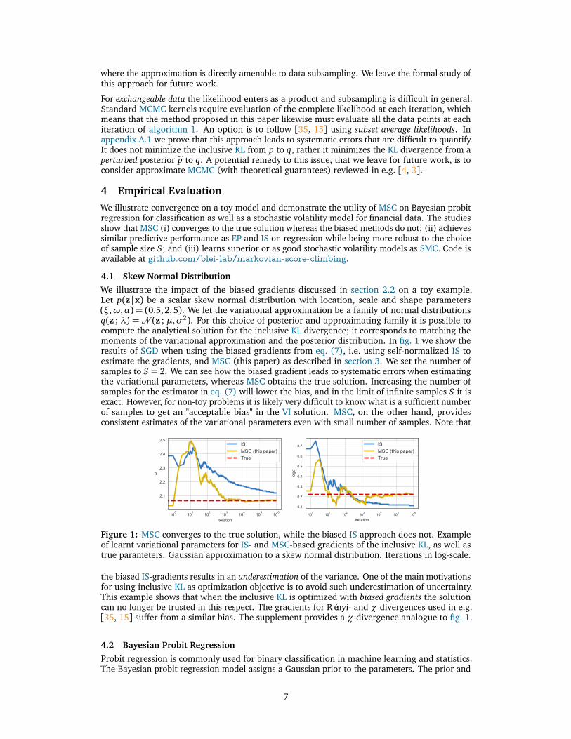
4.1 Skew Normal DistributionWe illustrate the impact of the biased gradients discussed in section 2.2 on a toy example.Let p(z |x) be a scalar skew normal distribution with location, scale and shape parameters(⇠,!,↵) = (0.5,2,5). We let the variational approximation be a family of normal distributionsq(z ; �) = N (z ; µ,�2). For this choice of posterior and approximating family it is possible tocompute the analytical solution for the inclusive KL divergence; it corresponds to matching themoments of the variational approximation and the posterior distribution. In fig. 1 we show theresults of SGD when using the biased gradients from eq. (7), i.e. using self-normalized IS toestimate the gradients, and MSC (this paper) as described in section 3. We set the number ofsamples to S = 2. We can see how the biased gradient leads to systematic errors when estimatingthe variational parameters, whereas MSC obtains the true solution. Increasing the number ofsamples for the estimator in eq. (7) will lower the bias, and in the limit of infinite samples S it isexact. However, for non-toy problems it is likely very difficult to know what is a sufficient numberof samples to get an "acceptable bias" in the VI solution. MSC, on the other hand, providesconsistent estimates of the variational parameters even with small number of samples. Note that
Figure 1: MSC converges to the true solution, while the biased IS approach does not. Exampleof learnt variational parameters for IS- and MSC-based gradients of the inclusive KL, as well astrue parameters. Gaussian approximation to a skew normal distribution. Iterations in log-scale.
the biased IS-gradients results in an underestimation of the variance. One of the main motivationsfor using inclusive KL as optimization objective is to avoid such underestimation of uncertainty.This example shows that when the inclusive KL is optimized with biased gradients the solutioncan no longer be trusted in this respect. The gradients for Rényi- and � divergences used in e.g.[35, 15] suffer from a similar bias. The supplement provides a � divergence analogue to fig. 1.
4.2 Bayesian Probit RegressionProbit regression is commonly used for binary classification in machine learning and statistics.The Bayesian probit regression model assigns a Gaussian prior to the parameters. The prior and
7
(a) Heart µ?1 (b) Heart µ?3 (c) Heart µ?4
(d) Ionos µ?1 (e) Ionos µ?17 (f) Ionos µ?27
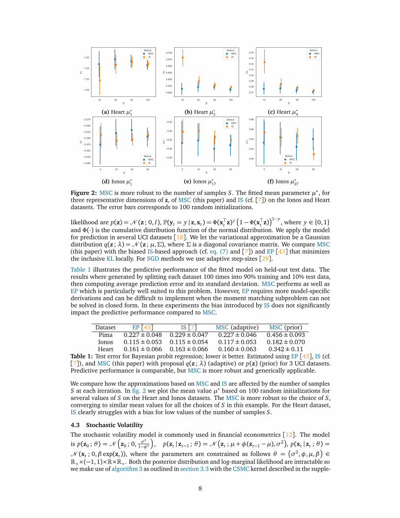
Figure 2: MSC is more robust to the number of samples S. The fitted mean parameter µ?, forthree representative dimensions of z, of MSC (this paper) and IS (cf. [7]) on the Ionos and Heartdatasets. The error bars corresponds to 100 random initializations.
likelihood are p(z) =N (z ; 0, I), P(yt = y |z,xt) = �(x>t z)y�1��(x>
tz)�1�y
, where y 2 {0,1}and �(·) is the cumulative distribution function of the normal distribution. We apply the modelfor prediction in several UCI datasets [18]. We let the variational approximation be a Gaussiandistribution q(z ; �) =N (z ; µ,⌃), where ⌃ is a diagonal covariance matrix. We compare MSC(this paper) with the biased IS-based approach (cf. eq. (7) and [7]) and EP [43] that minimizesthe inclusive KL locally. For SGD methods we use adaptive step-sizes [29].
Table 1 illustrates the predictive performance of the fitted model on held-out test data. Theresults where generated by splitting each dataset 100 times into 90% training and 10% test data,then computing average prediction error and its standard deviation. MSC performs as well asEP which is particularly well suited to this problem. However, EP requires more model-specificderivations and can be difficult to implement when the moment matching subproblem can notbe solved in closed form. In these experiments the bias introduced by IS does not significantlyimpact the predictive performance compared to MSC.
Dataset EP [43] IS [7] MSC (adaptive) MSC (prior)Pima 0.227± 0.048 0.229± 0.047 0.227± 0.046 0.456± 0.093Ionos 0.115± 0.053 0.115± 0.054 0.117± 0.053 0.182± 0.070Heart 0.161± 0.066 0.163± 0.066 0.160± 0.063 0.342± 0.11
Table 1: Test error for Bayesian probit regression; lower is better. Estimated using EP [43], IS (cf.[7]), and MSC (this paper) with proposal q(z ; �) (adaptive) or p(z) (prior) for 3 UCI datasets.Predictive performance is comparable, but MSC is more robust and generically applicable.
We compare how the approximations based on MSC and IS are affected by the number of samplesS at each iteration. In fig. 2 we plot the mean value µ? based on 100 random initializations forseveral values of S on the Heart and Ionos datasets. The MSC is more robust to the choice of S,converging to similar mean values for all the choices of S in this example. For the Heart dataset,IS clearly struggles with a bias for low values of the number of samples S.
4.3 Stochastic VolatilityThe stochastic volatility model is commonly used in financial econometrics [12]. The modelis p(z0 ; ✓ ) = N
Äz0 ; 0, �2
1��2
ä, p(zt |zt�1 ; ✓ ) = N
�zt ; µ+�(zt�1 �µ),�2
�, p(xt |zt ; ✓ ) =
N (xt ; 0,� exp(zt)), where the parameters are constrained as follows ✓ =��2,�,µ,��2
R+⇥(�1, 1)⇥R⇥R+. Both the posterior distribution and log-marginal likelihood are intractable sowe make use of algorithm 3 as outlined in section 3.3 with the CSMC kernel described in the supple-
8
ment. The proposal distributions are q(z0 ; ✓ ,�0)/ p(z0 ; ✓ )e�12⇤0z2
0+⌫0z0 , q(zt |zt�1 ; ✓ ,�t)/p(zt |zt�1 ; ✓ ) e�
12⇤t z2
t+⌫t zt , with variational parameters �t = (⌫t ,⇤t) 2 R ⇥ R+.
1 2 3 4 5 6 7 8 9 10 11 12 13 14 15 16 17 18Dataset
0
5
10
15
20
log
p(x
1:T
;�� M
SC)�
log
p(x
1:T
;�� SM
C)
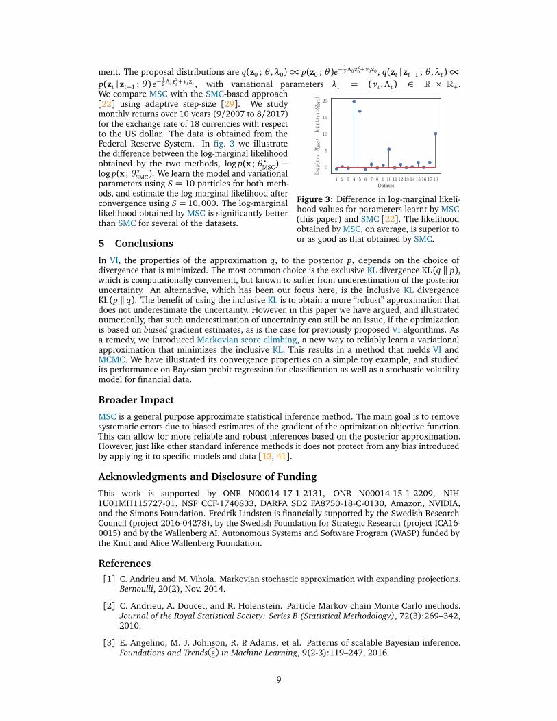
Figure 3: Difference in log-marginal likeli-hood values for parameters learnt by MSC(this paper) and SMC [22]. The likelihoodobtained by MSC, on average, is superior toor as good as that obtained by SMC.
We compare MSC with the SMC-based approach[22] using adaptive step-size [29]. We studymonthly returns over 10 years (9/2007 to 8/2017)for the exchange rate of 18 currencies with respectto the US dollar. The data is obtained from theFederal Reserve System. In fig. 3 we illustratethe difference between the log-marginal likelihoodobtained by the two methods, log p(x ; ✓?MSC) �log p(x ; ✓?SMC). We learn the model and variationalparameters using S = 10 particles for both meth-ods, and estimate the log-marginal likelihood afterconvergence using S = 10,000. The log-marginallikelihood obtained by MSC is significantly betterthan SMC for several of the datasets.
5 ConclusionsIn VI, the properties of the approximation q, to the posterior p, depends on the choice ofdivergence that is minimized. The most common choice is the exclusive KL divergence KL (q k p),which is computationally convenient, but known to suffer from underestimation of the posterioruncertainty. An alternative, which has been our focus here, is the inclusive KL divergenceKL (p k q). The benefit of using the inclusive KL is to obtain a more “robust” approximation thatdoes not underestimate the uncertainty. However, in this paper we have argued, and illustratednumerically, that such underestimation of uncertainty can still be an issue, if the optimizationis based on biased gradient estimates, as is the case for previously proposed VI algorithms. Asa remedy, we introduced Markovian score climbing, a new way to reliably learn a variationalapproximation that minimizes the inclusive KL. This results in a method that melds VI andMCMC. We have illustrated its convergence properties on a simple toy example, and studiedits performance on Bayesian probit regression for classification as well as a stochastic volatilitymodel for financial data.
Broader ImpactMSC is a general purpose approximate statistical inference method. The main goal is to removesystematic errors due to biased estimates of the gradient of the optimization objective function.This can allow for more reliable and robust inferences based on the posterior approximation.However, just like other standard inference methods it does not protect from any bias introducedby applying it to specific models and data [13, 41].
Acknowledgments and Disclosure of FundingThis work is supported by ONR N00014-17-1-2131, ONR N00014-15-1-2209, NIH1U01MH115727-01, NSF CCF-1740833, DARPA SD2 FA8750-18-C-0130, Amazon, NVIDIA,and the Simons Foundation. Fredrik Lindsten is financially supported by the Swedish ResearchCouncil (project 2016-04278), by the Swedish Foundation for Strategic Research (project ICA16-0015) and by the Wallenberg AI, Autonomous Systems and Software Program (WASP) funded bythe Knut and Alice Wallenberg Foundation.
References[1] C. Andrieu and M. Vihola. Markovian stochastic approximation with expanding projections.
Bernoulli, 20(2), Nov. 2014.
[2] C. Andrieu, A. Doucet, and R. Holenstein. Particle Markov chain Monte Carlo methods.Journal of the Royal Statistical Society: Series B (Statistical Methodology), 72(3):269–342,2010.
[3] E. Angelino, M. J. Johnson, R. P. Adams, et al. Patterns of scalable Bayesian inference.Foundations and Trends R� in Machine Learning, 9(2-3):119–247, 2016.
9
[4] R. Bardenet, A. Doucet, and C. Holmes. On Markov chain Monte Carlo methods for talldata. Journal of Machine Learning Research, 18(47):1–43, 2017.
[5] A. Benveniste, M. Métivier, and P. Priouret. Adaptive algorithms and stochastic approximations,volume 22. Springer Science & Business Media, 1990.
[6] D. Blei, A. Kucukelbir, and J. D. McAuliffe. Variational inference: A review for statisticians.Journal of the American statistical Association, 112(518):859–877, 2017.
[7] B. Bornschein and Y. Bengio. Reweighted wake-sleep. In International Conference on
Learning Representations, 2015.
[8] M. F. Bugallo, V. Elvira, L. Martino, D. Luengo, J. Miguez, and P. M. Djuric. Adaptiveimportance sampling: the past, the present, and the future. IEEE Signal Processing Magazine,34(4):60–79, 2017.
[9] Y. Burda, R. Grosse, and R. Salakhutdinov. Importance weighted autoencoders. In Interna-
tional Conference on Learning Representations, 2016.
[10] O. Cappé, A. Guillin, J.-M. Marin, and C. P. Robert. Population Monte Carlo. Journal of
Computational and Graphical Statistics, 13(4):907–929, 2004.
[11] O. Cappé, R. Douc, A. Guillin, J.-M. Marin, and C. P. Robert. Adaptive importance samplingin general mixture classes. Statistics and Computing, 18(4):447–459, 2008.
[12] S. Chib, Y. Omori, and M. Asai. Multivariate Stochastic Volatility, pages 365–400. SpringerBerlin Heidelberg, Berlin, Heidelberg, 2009.
[13] S. Corbett-Davies and S. Goel. The measure and mismeasure of fairness: A critical reviewof fair machine learning. arXiv:1808.00023, 2018.
[14] A. B. Dieng and J. Paisley. Reweighted expectation maximization. arXiv:1906.05850, 2019.
[15] A. B. Dieng, D. Tran, R. Ranganath, J. Paisley, and D. Blei. Variational inference via chiupper bound minimization. In Advances in Neural Information Processing Systems 30, pages2732–2741. Curran Associates, Inc., 2017.
[16] J. Domke and D. R. Sheldon. Divide and couple: Using Monte Carlo variational objectivesfor posterior approximation. In Advances in Neural Information Processing Systems, pages338–347, 2019.
[17] R. Douc, A. Guillin, J.-M. Marin, C. P. Robert, et al. Convergence of adaptive mixtures ofimportance sampling schemes. The Annals of Statistics, 35(1):420–448, 2007.
[18] D. Dua and C. Graff. UCI machine learning repository, 2017. URL http://archive.ics.uci.edu/ml.
[19] A. Finke and A. H. Thiery. On importance-weighted autoencoders. arXiv:1907.10477, 2019.
[20] Z. Ghahramani and M. J. Beal. Propagation algorithms for variational Bayesian learning.In Advances in neural information processing systems, pages 507–513, 2001.
[21] M. G. Gu and F. H. Kong. A stochastic approximation algorithm with Markov chain Monte-Carlo method for incomplete data estimation problems. Proceedings of the National Academy
of Sciences, 95(13):7270–7274, 1998.
[22] S. S. Gu, Z. Ghahramani, and R. E. Turner. Neural adaptive sequential Monte Carlo. InAdvances in Neural Information Processing Systems 28, pages 2629–2637. Curran Associates,Inc., 2015.
[23] P. Guarniero, A. M. Johansen, and A. Lee. The iterated auxiliary particle filter. Journal of
the American Statistical Association, 112(520):1636–1647, 2017.
[24] R. Habib and D. Barber. Auxiliary variational MCMC. In International Conference on Learning
Representations, 2019.
10
[25] J. Heng, A. N. Bishop, G. Deligiannidis, and A. Doucet. Controlled sequential Monte Carlo.arXiv:1708.08396, 2017.
[26] M. Hoffman, P. Sountsov, J. V. Dillon, I. Langmore, D. Tran, and S. Vasudevan. Neutra-lizingbad geometry in Hamiltonian Monte Carlo using neural transport. arXiv:1903.03704, 2019.
[27] M. D. Hoffman. Learning deep latent Gaussian models with Markov chain Monte Carlo. InProceedings of the 34th International Conference on Machine Learning, pages 1510–1519,2017.
[28] M. I. Jordan, Z. Ghahramani, T. S. Jaakkola, and L. K. Saul. An introduction to variationalmethods for graphical models. Machine Learning, 37(2):183–233, Nov. 1999.
[29] D. P. Kingma and J. Ba. Adam: A method for stochastic optimization. arXiv preprint
arXiv:1412.6980, 2014.
[30] D. P. Kingma and M. Welling. Auto-encoding variational Bayes. In International Conference
on Learning Representations, 2014.
[31] E. Kuhn and M. Lavielle. Coupling a stochastic approximation version of EM with an MCMCprocedure. ESAIM: Probability and Statistics, 8:115–131, 2004.
[32] H. Kushner and G. G. Yin. Stochastic approximation and recursive algorithms and applications,volume 35. Springer Science & Business Media, 2003.
[33] D. Lawson, G. Tucker, C. A. Naesseth, C. Maddison, and Y. Whye Teh. Twisted variationalsequential Monte Carlo. Third workshop on Bayesian Deep Learning (NeurIPS), 2018.
[34] T. A. Le, M. Igl, T. Rainforth, T. Jin, and F. Wood. Auto-encoding sequential Monte Carlo. InInternational Conference on Learning Representations, 2018.
[35] Y. Li and R. E. Turner. Rényi divergence variational inference. In Advances in Neural
Information Processing Systems 29, pages 1073–1081. Curran Associates, Inc., 2016.
[36] Y. Li, R. E. Turner, and Q. Liu. Approximate inference with amortised MCMC.arXiv:1702.08343, 2017.
[37] A. Lindholm and F. Lindsten. Learning dynamical systems with particle stochastic approxi-mation em. arXiv:1806.09548, 2019.
[38] F. Lindsten, M. I. Jordan, and T. B. Schön. Particle Gibbs with ancestor sampling. The
Journal of Machine Learning Research, 15(1):2145–2184, 2014.
[39] F. Lindsten, J. Helske, and M. Vihola. Graphical model inference: Sequential Monte Carlomeets deterministic approximations. In Advances in Neural Information Processing Systems
31, pages 8201–8211. Curran Associates, Inc., 2018.
[40] C. J. Maddison, D. Lawson, G. Tucker, N. Heess, M. Norouzi, A. Mnih, A. Doucet, andY. Whye Teh. Filtering variational objectives. In Advances in Neural Information Processing
Systems, 2017.
[41] N. Mehrabi, F. Morstatter, N. Saxena, K. Lerman, and A. Galstyan. A survey on bias andfairness in machine learning. arXiv:1908.09635, 2019.
[42] T. Minka. Divergence measures and message passing. Technical report, Technical report,Microsoft Research, 2005.
[43] T. P. Minka. Expectation propagation for approximate Bayesian inference. In Proceedings of
the Seventeenth conference on Uncertainty in artificial intelligence, pages 362–369. MorganKaufmann Publishers Inc., 2001.
[44] A. K. Moretti, Z. Wang, L. Wu, I. Drori, and I. Pe’er. Particle smoothing variational objectives.arXiv:1909.09734, 2019.
11
[45] C. A. Naesseth, F. J. R. Ruiz, S. W. Linderman, and D. Blei. Reparameterization gradientsthrough acceptance-rejection sampling algorithms. In Proceedings of the 20th International
Conference on Artificial Intelligence and Statistics, 2017.
[46] C. A. Naesseth, S. Linderman, R. Ranganath, and D. Blei. Variational sequential MonteCarlo. In International Conference on Artificial Intelligence and Statistics, volume 84, pages968–977. PMLR, 2018.
[47] C. A. Naesseth, F. Lindsten, and T. B. Schön. Elements of sequential Monte Carlo. Foundations
and Trends R� in Machine Learning, 12(3):307–392, 2019.
[48] Z. Ou and Y. Song. Joint stochastic approximation and its application to learning discretelatent variable models. In Conference on Uncertainty in Artificial Intelligence (UAI), 2020.
[49] A. B. Owen. Monte Carlo theory, methods and examples. 2013.
[50] B. Paige and F. Wood. Inference networks for sequential Monte Carlo in graphical models.In International Conference on Machine Learning, pages 3040–3049, 2016.
[51] J. W. Paisley, D. Blei, and M. I. Jordan. Variational Bayesian inference with stochastic search.In International Conference on Machine Learning, 2012.
[52] R. Ranganath, S. Gerrish, and D. Blei. Black box variational inference. In Artificial Intelligence
and Statistics, 2014.
[53] D. J. Rezende, S. Mohamed, and D. Wierstra. Stochastic backpropagation and approximateinference in deep generative models. In International Conference on Machine Learning,2014.
[54] H. Robbins and S. Monro. A stochastic approximation method. The Annals of Mathematical
Statistics, pages 400–407, 1951.
[55] C. Robert and G. Casella. Monte Carlo statistical methods. Springer Science & BusinessMedia, 2004.
[56] F. J. R. Ruiz and M. K. Titsias. A contrastive divergence for combining variational inferenceand MCMC. In Proceedings of the 36th International Conference on Machine Learning, pages5537–5545, 2019.
[57] F. J. R. Ruiz, M. K. Titsias, and D. Blei. The generalized reparameterization gradient. InAdvances in Neural Information Processing Systems, 2016.
[58] T. Salimans and D. A. Knowles. Fixed-form variational posterior approximation throughstochastic linear regression. Bayesian Analysis, 8(4):837–882, 2013.
[59] T. Salimans, D. Kingma, and M. Welling. Markov chain Monte Carlo and variationalinference: Bridging the gap. In International Conference on Machine Learning, pages 1218–1226, 2015.
[60] R. E. Turner and M. Sahani. Two problems with variational expectation maximisation fortime-series models. In D. Barber, A. T. Cemgil, and S. Chiappa, editors, Bayesian time series
models, chapter 5, pages 109–130. Cambridge University Press, 2011.
[61] T. Wang, Y. Wu, D. Moore, and S. J. Russell. Meta-learning MCMC proposals. In Advances
in neural information processing systems, pages 4146–4156, 2018.
[62] H. Wu, H. Zimmermann, E. Sennesh, T. A. Le, and J.-W. van de Meent. Inference networksfor sequential Monte Carlo in graphical models. In International Conference on Machine
Learning, 2020.
12