Embed Size (px)
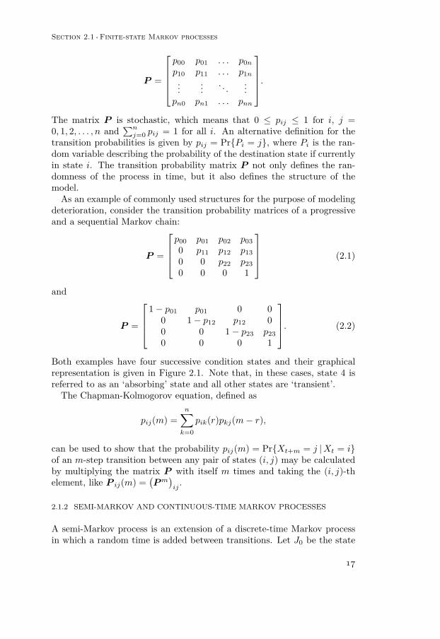
Citation preview

Cite this document as:
M.J. Kallen. Markov processes for maintenance optimization of civil infra-structure in the Netherlands. Ph.D. thesis, Delft University of Technology,Delft, 2007.
BibTEX entry:
@phdthesis{kallen2007phd,author = {Kallen, M. J.},title = {Markov processes for maintenance optimization of
civil infrastructure in the Netherlands},year = {2007},school = {Delft University of Technology},address = {Delft, Netherlands},ISBN = {978-90-770051-29-0}
}


MARKOV PROCESSES FORMAINTENANCE OPTIMIZATION OF CIVIL
INFRASTRUCTURE IN THE NETHERLANDS
M.J. Kallen


MARKOV PROCESSES FORMAINTENANCE OPTIMIZATION OF CIVIL
INFRASTRUCTURE IN THE NETHERLANDS
Proefschrift
ter verkrijging van de graad van doctoraan de Technische Universiteit Delft,
op gezag van de Rector Magnificus prof. dr. ir. Jacob Fokkema,voorzitter van het College voor Promoties,
in het openbaar te verdedigen op dinsdag 4 december 2007 om 10.00 uurdoor Maarten-Jan KALLEN
wiskundig ingenieurgeboren te Creve Coeur, Verenigde Staten van Amerika.

Dit proefschrift is goedgekeurd door de promotor:
Prof. dr. ir. J.M. van Noortwijk
Samenstelling promotiecommissie:
Rector Magnificus, VoorzitterProf. dr. ir. J.M. van Noortwijk, Technische Universiteit Delft, promotorProf. dr. D.M. Frangopol, Lehigh UniversityProf. dr. A. Grall, Université de Technologie de TroyesProf. dr. ir. R. Dekker, Erasmus Universiteit RotterdamProf. dr. T.A. Mazzuchi, George Washington UniversityProf. dr. ir. G. Jongbloed, Technische Universiteit DelftDr. ir. A. van Beek, Vereniging van Ondernemingen van
Betonmortelfabrikanten in NederlandProf. dr. R.M. Cooke, Technische Universiteit Delft, reservelid
Dit proefschrift is tot stand gekomen met ondersteuning van de Bouw-dienst Rijkswaterstaat, HKV Lijn in water en de faculteit Electrotechniek,Wiskunde en Informatica van de Technische Universiteit Delft.
ISBN 978–90–770051–29–0
Copyright C© 2007 by M.J. Kallen
Cover design by Jan van Dijk, DratexOn the cover: the ‘Van Galecopper’ bridge in Utrecht
Typeset with ConTEXtPrinted in The Netherlands

i
Contents
Summary iii · Samenvatting v
1 Introduction 11.1 Bridge management 21.2 Maintenance modeling 31.3 Bridges and their inspection in the Netherlands 61.4 Aim of research 111.5 Reading guide 12
2 Markov processes for bridge deterioration 152.1 Finite-state Markov processes 152.2 Characteristics of bridge inspection data 222.3 Review of statistical models and estimation methods 252.4 Testing the Markov property 402.5 Using semi-Markov processes 41
3 Proposed framework 453.1 Maximum likelihood estimation 453.2 Statistical model 473.3 Maximization 523.4 Data requirements for model application 55
4 Application and results 574.1 Dutch bridge condition data 574.2 Selection of transition structure 624.3 Inclusion of inspection variability 794.4 Analysis of covariate influence 82
5 Optimal maintenance decisions 875.1 Markov decision processes 875.2 Condition-based inspection and maintenance model 885.3 Survival probability 101
6 Conclusions and recommendations 105
7 Appendix: transition probability function 1137.1 Homogeneous Markov processes 1137.2 Non-homogeneous Markov processes 1177.3 Parameter sensitivity 124
References 131 · Acknowledgments 139 · About the author 141


iii
Summary
The Netherlands, like many countries in this world, face a challenging taskin managing civil infrastructures. The management of vital infrastructures,like road bridges, is necessary to ensure their safe and reliable functioning.Various material restrictions, of which limited budgets are the most obviousexample, require that the costs of inspections and maintenance must bebalanced against their benefits.
A principal element of bridge management systems is the estimation ofthe uncertain rate of deterioration. This is usually done by using a suit-able model and by using information gathered on-site. The primary sourceof information are visual inspections performed periodically. It is mainlydue to the large number of bridges that these are not continuously moni-tored, but there are many other reasons why monitoring of all bridges isnot practically feasible. The periodic nature of inspections creates specificrequirements for the deterioration model.
This thesis proposes a statistical and probabilistic framework, whichenables the decision maker to estimate the rate of deterioration and toquantify his uncertainty about this estimate. The framework consists of acontinuous-time Markov process with a finite number of states to model theuncertain rate at which the quality of structures reduces over time. Theparameters of the process are estimated using the method of maximumlikelihood and the likelihood function is defined such that the dependencebetween the condition at two successive inspections is properly accountedfor.
The results of the model show that it is applicable even if the data aresubject to inspector interpretation error. Based on a data set of generalconditions of bridges in the Netherlands, they are expected to require majorrenovation after approximately 45 to 50 years of service. This is roughlyhalfway the intended lifetime at design. The results also show significantuncertainty in the estimates, which is due to the large variability in anumber of factors. These factors include the design of the structures, thequality of the construction material, the workmanship of the contractor,the influence of the weather, and the increasing intensity and weight oftraffic.
A condition-based inspection model, specifically tailored to finite-stateMarkov processes, is proposed. It allows the decision maker to determinethe time between inspections with the lowest expected average costs peryear. The model, also known as the functional or marginal check-model,is based on renewal theory and therefore constitutes a life-cycle approachto the optimization of inspections and maintenance. In addition to this, a

iv
complete chapter is devoted to determining the most computationally effec-tive way of performing the necessary calculations in the deterioration anddecision models. This ensures that analyses can be done almost instantly,even for very large numbers of structures.
The unified framework to deterioration modeling and decision makingpresented herein, contributes a quantitative approach to bridge manage-ment in the Netherlands and to infrastructure management in general. Itcan be applied to other fields of similar character like, for example, pave-ment and sewer system management.

v
Samenvatting
Nederland, zoals vele landen in deze wereld, staat voor een uitdagendetaak in het beheer van civiele infrastructuur. Het beheer van belangrijkekunstwerken, zoals bruggen in het wegennet, is noodzakelijk om deze veiligen betrouwbaar te laten functioneren. Vanwege verschillende materiëlerestricties moeten de kosten van inspecties en onderhoud afgewogen wordentegen de baten. De meest voordehandliggende restrictie is die van eenbeperkt budget.
De schatting van de onzekere snelheid van veroudering is het belangrijk-ste element in een beheersysteem voor bruggen. Dit wordt gewoonlijkgedaan door gebruik te maken van een geschikt model en van gegevensdie op lokatie zijn verzameld. De voornamelijkste bron van informatie zijnvisuele inspecties die de beheerder periodiek laat uitvoeren. Het is vooralvanwege het grote aantal bruggen dat deze niet continu gemeten worden,maar er zijn veel meer redenen waarom dit in de praktijk niet haalbaaris. Het feit dat kunstwerken slechts periodiek geïnspecteerd worden, steltbijzondere eisen aan het verouderingsmodel.
Dit proefschrift beschrijft een statistische en probabilistische aanpak diehet de beheerder mogelijk maakt om de snelheid van veroudering te schat-ten en ook om zijn onzekerheid over deze schatting te kwantificeren. Hetmodel bestaat uit een continue-tijd Markov proces met een eindig aan-tal toestanden om de onzekere snelheid van veroudering van kunstwerkenover tijd te beschrijven. De parameters van dit model worden geschatdoor gebruik te maken van de methode van de grootste aannemelijkheid.De functie voor de aannemelijkheid is zodanig gedefinieerd dat deze deafhankelijkheid tussen twee opeenvolgende inspecties correct meeneemt.
De resultaten van het model tonen aan dat deze goed toepasbaar is,zelfs als de gegevens onderhavig zijn aan fouten die zijn gemaakt doorde inspecteurs. Gebaseerd op een bestand van de algemene conditie vanbruggen, hebben deze naar verwachting op een leeftijd van ongeveer 45 tot50 jaar een grondige renovatie nodig. Dit is ruwweg halverwege de beoogdelevensduur bij het ontwerp van een brug. De resultaten tonen ook een groteonzekerheid in de voorspelling, hetgeen komt door de grote variabiliteit ineen aantal factoren. Voorbeelden van zulke factoren zijn het ontwerp vande kunstwerken, het vakmanschap van de aannemer, de kwaliteit van hetmateriaal, de invloed van het weer, en de toename in intensiteit en gewichtvan het verkeer.
Een toestandsafhankelijk inspectiemodel, die geschikt is voor Markovprocessen met een eindig aantal toestanden, wordt gepresenteerd aan heteinde van dit proefschrift. Het staat de beheerder toe om de tijd tusseninspecties te bepalen met de laagst verwachte gemiddelde kosten per jaar.

vi
Dit model is gebaseerd op vernieuwingstheorie en beschouwd daarom dehele levenscyclus van het kunstwerk bij de optimalisatie van inspecties enonderhoud. Daarbovenop wordt een volledig hoofdstuk gewijd aan hetbepalen van de meest efficiënte manier om de noodzakelijke berekeningenin het verouderings- en beslismodel uit te voeren. Dit zorgt ervoor dat deanalyses in heel korte tijd uitgevoerd kunnen worden, zelfs voor een heelgroot aantal kunstwerken.
Het complete concept voor het modelleren van veroudering en het ne-men van beslissingen voor optimaal onderhoud, zoals deze in dit proefschriftbeschreven worden, voegt een gedegen kwantitatieve aanpak toe aan hetbrugbeheer in Nederland en aan het beheer en onderhoud van civiele infra-structuur in het algemeen. Het kan toegepast worden in andere gebiedenvan een vergelijkbaar karakter, zoals bijvoorbeeld bij het beheer en onder-houd van asfaltering en riolering.

1
1Introduction
In the year 2007, several bridges have made it into the news. Unfortunately,the news was not good. On August 1st, the I-35W Mississippi River Bridgein Minneapolis, Minnesota in the United States of America, collapsed dur-ing heavy traffic, killing 13 people. The images from the wreckage of thesteel bridge were broadcast worldwide by television and internet. Theyshowed the devastation resulting from the collapse of such a large struc-ture.
On August 13th, an almost completed concrete bridge over the Tuo rivernear Fenghuang in the people’s republic of China, collapsed killing 22 con-struction workers. Incidentally, the collapse occurred on the same day theChinese government announced a plan to renovate over 6000 bridges whichare known to be structurally unsafe.
In April, people in the Netherlands were confronted with the extremelyrare announcement that a bridge would be closed for heavy traffic dueto concerns about its load carrying capacity. This bridge, the ‘Hollandsebrug’, is part of a highway connecting the cities of Amsterdam and Almere.
Bridges and viaducts play a vital role in today’s transportation infra-structure and therefore are essential to today’s economy. They are con-structed and maintained in order to reliably fulfill this role, while alsoensuring the safety of the passing traffic. However, most countries nowa-days face an aging bridge stock and a strong increase in traffic. This makesbridge management a challenging problem, especially when budgets formaintenance are generally shrinking.
Aside from the loss of human life and the emotional impact of cata-strophic incidents with bridges, the monetary costs can be extremely highas well. According to an estimate by the transportation industry in theNetherlands, the cost of the closure of the ‘Hollandse brug’ could run upto around ¤160 000 per day. The reconstruction of the Mississippi RiverBridge was recently awarded for an amount of $238 million. The totalcosts of the bridge collapse, including the reconstruction, rescue efforts,and clean up, are estimated to be approximately $393 million by the Min-nesota Department of Transportation.
There are many factors which make bridge management a complex prob-lem. These include the occurrence of changes in construction methods andbuilding codes over the years, the varying weight and intensity of traffic, the

Chapter 1 · Introduction
2
large number of structures over a large area, the influence of the weather onthe structure, and many more. These factors have one thing in common:they create uncertainty. The problem of bridge management is therefore aproblem of decision-making under uncertainty. The uncertainty primarilylies in the lifetime of the structures. Over the years, many efforts have beenmade to better predict deterioration in bridges of all sorts in order to moreeffectively perform the maintenance of bridges.
The research presented in this thesis is aimed at modeling the rate ofdeterioration of bridges in the Netherlands. This is done by using informa-tion on the condition of bridges obtained by inspections performed between1985 and 2004. A very large number of bridges in the Netherlands wereconstructed during the 1960’s and 1970’s. The design life of bridges is gen-erally around 80 to 100 years. In the Netherlands, by experience, bridgesrequire a major renovation approximately halfway their operational life.This means that the country is soon facing a wave of structures which arein need of renovation.
The remainder of this chapter provides a general introduction to bridgemanagement and how maintenance modeling is used as part of this. Thereare many different types of mathematical models available, which can beused for the purpose of determining optimal maintenance policies. In Sec-tion 1.3, an overview is given of the current bridge management practicesin the Netherlands and why one particular modeling approach, namely onethat uses a finite-state Markov process for modeling the uncertain deterio-ration, is particularly suitable for application in the Netherlands.
1.1 BRIDGE MANAGEMENT
Bridge management is the general term used for the optimal planning ofinspections and maintenance of road bridges. Most management systemswill consider the bridges as a node in a road network in order to reduceunnecessary traffic obstructions and the number of maintenance actions.The necessity for bridge management systems (BMS) has grown in recentyears. The construction of new bridges is slowing down and older bridgesare starting to reach a critical age of about 40 years at which major mainte-nance and renovation work is necessary. Due to budget constraints, bridgeowners are focusing increasingly on maintenance and repair instead of re-placement.
Maintenance models are developed and used to balance the costs againstthe benefits (e.g., increased safety) of current and future maintenance andrepair actions. A bridge maintenance system increases the scope of theanalysis to the planning of maintenance for a network of bridges. QuotingScherer and Glagola (1994): ‘A BMS is defined as a rational and systematic

Section 1.2 ·Maintenance modeling
3
approach to organizing and carrying out all the activities related to manag-ing a network of bridges’. The goal of this approach is the following: ‘Theobjective of a BMS is to preserve the asset value of the infrastructure byoptimizing costs over the lifespan of the bridges, while ensuring the safetyof users and by offering a sufficient quality of service’, which is quoted fromWoodward et al. (2001).
Individual bridges are complex structures made up of multiple compo-nents and are constructed using several material types. Their structuralbehavior, the quality of the construction materials, and the intensity of traf-fic loads, are highly uncertain. Many models have been proposed to betterpredict the overall deterioration of bridges and to schedule inspections andmaintenance such that costs and safety are optimally balanced.
1.2 MAINTENANCE MODELING
Maintenance, or the act of maintaining something, is defined as ‘ensuringthat physical assets continue to do what their users want them to do’by Moubray (1997). More formally, maintenance consists of any activityto restore or retain a functional unit in a specified state such that it isable to perform its required functions. The general goal of maintenanceoptimization may be formulated as ‘the optimal execution of maintenanceactivities subject to one or more constraints’. In this definition, there arethree aspects: what is optimal, what maintenance activities are available,and which constraints must be respected? An obvious constraint is a finitebudget, which means that structures can not simply be replaced at any timeand that maintenance can not be performed continuously. Constraints onthe availability of construction material and qualified personnel may alsocreate restrictions. There are many examples of maintenance, which maybe small (like cleaning drainage holes) or large (like resurfacing the bridgedeck), but inspections also represent an important activity. Inspectionshelp gather information for making decisions and their results may influencefuture maintenance and therefore also the future condition of structures.This information is subsequently used in the last aspect to be discussedhere, namely the aspect of optimization. Maintenance and inspectionsmay be performed such that the costs are minimized, the reliability oravailability maximized, the safety maximized, or that a combination ofthese is optimal in some way.
The challenging aspect of maintenance optimization, is that the state ofa structure can not be accurately predicted throughout its lifetime. Thetime to reach a deficient condition is uncertain and varies strongly betweendifferent structures. This uncertainty is a result of many factors, includingthe quality of the construction material, the quality of the workmanship,the traffic intensity and the stress which is put onto the structure by heavy

Chapter 1 · Introduction
4
6 6
6 6
maintenance model
data deteriorationmodel
decisionmodel
optimal policy
Figure 1.1: Simple representation of thetwo basic elements of a maintenance model:the deterioration and decision models.
loads. A natural variability exists due to for example differences in temper-ature, rainfall, wind and the presence of salt (e.g., in a maritime climate orin areas where frequent use of deicing salt is required). In order to make asound decision on which maintenance policy is to be applied, the decisionmaker can use a model which represents an abstraction of reality and whichquantifies the uncertainties involved in the degradation process. From this,it is obvious that such a model should be probabilistic in nature and notdeterministic.
1.2.1 ELEMENTS OF A MAINTENANCE OPTIMIZATION MODEL
Maintenance models may be roughly divided in two parts: a deteriorationmodel and a decision model. These two elements, as shown in Figure 1.1,are the basic parts in any maintenance model.
The deterioration model represents the abstraction of the actual degra-dation and the decision model uses the predicted deterioration to determinewhich maintenance policy is optimal. The decision model incorporates thedecision criteria selected by the decision maker and uses information like,for example, costs of repair and the effectiveness of repair to calculate theoptimal policy. Typical decision criteria are the inspection interval, con-dition thresholds for preventive repair, and the type of maintenance suchas a complete renewal or a partial repair. Most of the variability and un-certainty is present in the deterioration model. The decision model mayincorporate some uncertainty in the costs of repair, the effectiveness of life-time extending maintenance, and in the discount rate, which is used todetermine the value of investments and costs in the future.
The deterioration model may be supplied with data which is availableto the decision maker. This data may include results from inspections inthe form of condition and damage measurements, but it may also consist ofestimates obtained using some form of expert judgment or a combinationof these. As there are typically many structures in a network, the data isstored in a database to which new data is regularly added.

Section 1.2 ·Maintenance modeling
5
1.2.2 PHYSICAL VERSUS STATISTICAL APPROACH
Modeling the progress of deterioration over time can be done by using aphysical or statistical approach. The physical approach entails the useof a model which attempts to exactly describe the deterioration processfrom a physical point of view. An example of such an approach is the useof Paris’ law for modeling the growth of cracks in steel plates. Anotherexample is the use of Fick’s second law of diffusion for modeling the rate ofpenetration of chlorides in concrete. This model was fitted by Gaal (2004)to measurements of the chloride content in concrete samples taken from 81bridges in the Netherlands.
A different approach to the problem of predicting deterioration based onhistorical data, is to assume that the data is generated by a mathematicalmodel which does not try to emulate reality. Most commonly, this willbe a probabilistic model which is fitted to the historical data by means ofstatistical estimation. An example of the statistical approach is the use oflifetime distributions fitted to lifetimes of bridges. This approach was usedby van Noortwijk and Klatter (2004), where a Weibull distribution is fittedto ages of existing and demolished bridges in the Netherlands. The natureof this approach necessarily means that there is no ‘true’ model, but onlymodels which fit better to the data compared to others; for example, seeLindsey (1996).
Other examples of the statistical approach are the application of stochas-tic processes like the gamma process and finite-state Markov processes. Thegamma process has been used to model various types of degradation like,for example, thinning of steel walls of pressurized vessels and pipelines inKallen and van Noortwijk (2005a) and the growth of scour holes in thesea-bed protection of a storm surge barrier in van Noortwijk et al. (1997).This process allows for a partial inclusion of physical knowledge by specify-ing the parameters in the expectation of the process, which is a power lawfunction. Finite-state Markov processes, like Markov chains, have beenused in the field of civil engineering to model uncertain deterioration ina number of areas like pavement, bridge, and sewer system management.One of the first examples is the Arizona pavement management system(Golabi et al., 1982), which inspired the Pontis bridge management system(Golabi and Shepard, 1997). More recently, Markov chains have been ap-plied to sewer system and water pipeline deterioration. For examples, seeWirahadikusumah et al. (2001) and Micevski et al. (2002). A more com-plete overview of the application of both gamma processes and finite-stateMarkov processes is given by Frangopol et al. (2004). A specific review ofthe application of gamma processes in maintenance models is given by vanNoortwijk (2007).

Chapter 1 · Introduction
6
1.2.3 LIFE-CYCLE COSTING
During the lifetime of a structure, the condition is influenced by many ex-ternal factors. The condition is also influenced by design decisions beforeconstruction, and maintenance actions after construction. Because everydecision influences the timing and the nature of future decisions, it is im-portant to take into account the effect of actions over the full lifetime ofthe structure. An important concept in infrastructure management is theconcept of ‘life-cycle costing’. All costs of construction, management anddemolition must be taken into account by the decision maker. Due to thelong design lives of bridges, the costs are usually discounted in time. Dis-counting is used to take into account the devaluation of money over time.The costs or rewards of future actions are therefore discounted towardstheir present value. Under the assumption that the costs of actions do notchange over time, the result of discounting is that future actions are lesscostly. Money which is not spent now, can earn interest until it is neededfor maintenance.
The timing of large scale repairs, like replacements, usually depends onthe state of the structure. For example, in an age-based maintenance policy,a structure is repaired at fixed age intervals or when a necessity arises,whichever occurs first. If the structure has reached a predefined failurecondition, it must be repaired or replaced. A common modeling approachis to use renewal theory which assumes that maintenance actions bring thestructure to an as-good-as-new state. In this case, a repair is thereforeequivalent to a replacement although it is usually not as expensive. Thekey idea behind renewal theory is that the timing of successive renewalsis increasingly uncertain and that the probability of a renewal per unit oftime will converge to a kind of average over the long run. As an example,the probability per year of a renewal using the Weibull lifetime distributionfor concrete bridges in the Netherlands, as determined by van Noortwijkand Klatter (2004), is shown in Figure 1.2. Renewal theory supplies thedecision maker with a number of convenient tools for the decision model ina maintenance model. A good theoretical presentation of renewal theoryis given by Ross (1970).
1.3 BRIDGES AND THEIR INSPECTION IN THE NETHERLANDS
The Dutch Directorate General for Public Works and Water Managementis responsible for the management of the national road infrastructure inthe Netherlands. The Directorate General forms a part of the Ministry ofTransport, Public Works and Water Management and consists of severalspecialist services. One of these is the Civil Engineering Division which isheadquartered in Utrecht, the Netherlands. The Civil Engineering Division

Section 1.3 ·Bridges and their inspection in the Netherlands
7
0 100 200 300 400 500
0.00
00.
010
0.02
0
time [yr]
den
sity
[−
]
Figure 1.2: Renewal density using an esti-mated lifetime distribution for road bridges inthe Netherlands.
‘develops, builds, maintains, advises and co-ordinates infrastructural andhydraulic engineering structures that are of social importance’.
Since January 1st, 2006, the Directorate General has received the statusof an agency within the ministry. The primary goal of this transformationis to apply a more businesslike approach to the execution of its tasks. Aspart of this new approach, the costs of business are weighed against theexpected benefits. In general, the goal is to increase the accountability byclearly specifying what work is to be done, how it is to be done, and at whatcost. Also, the satisfaction of the customer (i.e., the government and thepeople of the Netherlands) has become an even more important criterion.The commercial aspect also means that more engineering-like tasks (e.g.,drawing and cost calculations) are outsourced to the market; that is, tocommercial parties.
The national road network in the Netherlands consists of around 3200kilometers of road, of which 2200 kilometers are highways. Within thisnetwork, there are approximately 3200 bridges, where the exact construc-tion year is unknown for a little over 100 of these. Almost all bridges andviaducts are primarily concrete structures. About one hundred are mainlysteel structures, aquaducts, or moveable bridges. The focus of this re-search is solely on concrete bridges, because form the largest group withinthe population. Also, the other structures can be considered as a fairlyinhomogeneous group. Many of these structures are very unique in theirdesign and construction.

Chapter 1 · Introduction
8
Figure 1.3: Map of the Netherlands withthe location of bridges which are managed bythe Civil Engineering Division.
A map of the Netherlands with the location of the bridges is shown inFigure 1.3. A histogram of the construction years for concrete bridges inthe Netherlands is presented in Figure 1.4. As can be observed in thisfigure, most bridges are currently between 30 and 40 years old. Theyhave a life expectancy of about 80 to 100 years when designed. Due toincreasing costs and a decrease in the availability of sufficient budgets forthe construction and replacement of bridges, the focus is shifting moreand more towards the efficient management of structures. The increasedimportance of infrastructure management has also resulted in the creationof a new ‘maintenance and inspection’ group within the Civil EngineeringDivision.
In the current inspection regime, large bridges (longer than 200 meters)are inspected every ten years, and smaller bridges every six years. Variablemaintenance actions, which are defined as maintenance actions outside thelong-term maintenance policy, are performed based on the condition of the

Section 1.3 ·Bridges and their inspection in the Netherlands
9
7 7
7 7
1925
–192
9
1930
–193
4
1935
–193
9
1940
–194
4
1945
–194
9
1950
–195
4
1955
–195
9
1960
–196
4
1965
–196
9
1970
–197
4
1975
–197
9
1980
–198
4
1985
–198
9
1990
–199
4
1995
–199
9
2000
–200
40%
5%
10%
15%
20%
Figure 1.4: Histogram of construction yearsof concrete bridges in the Netherlands.
structures as observed during an inspection and routine maintenance isperformed every year.
There are two types of inspections: functional and technical inspections.The functional inspections are performed more frequently and are primar-ily focused on analyzing the extent of individual damages or the state ofmaterials. These functional inspections are usually performed by the re-gional office who is responsible for the structure. A technical inspection is athorough analysis of the complete structure, aimed at registering the pres-ence and severity of damages and at assessing the overall condition of thestructure. The information gained from the technical inspections is usedby the Civil Engineering Division for the purpose of managing the struc-tures in the national road network. For this reason, and due to the factthat these inspections require specialized knowledge, the Civil EngineeringDivision is responsible for the planning and execution of these inspections.
The information gathered in a technical inspection is registered in an elec-tronic database. The database includes the basic information of all struc-tures in the Netherlands. This includes details like the location (province,community, highway, geographical coordinates, etc.), the size (length andwidth), if it is part of the highway or if it is located over the highway,the construction year, and which regional office of the Civil EngineeringDivision is responsible for regular inspections and maintenance.

Chapter 1 · Introduction
10
9 9
9 9
complex
functionalstructure
logical structure
principal parts
basic elements
Figure 1.5: The relationship of structuresand their elements in the Dutch bridge inspec-tion database.
The largest objects in the database are the complexes, which may consistof one or more structures (e.g., different spans in a long bridge or two paral-lel bridges). Complexes are divided in two ways: functional or logical. Thefunctional sectioning separates structures with different limits on trafficwidth, height and weight within the complex. This information is primar-ily used for the planning of special convoys which are particularly large orheavy. The logical separation is used for inspection purposes and separatesthe parts in the complex by the expertise which is required for the inspec-tions. This means that, for example, all concrete, steel, moveable parts,and electrical components are considered as separate units for inspections.Each of these ‘structures’ is further divided in principal parts like for exam-ple, the superstructure of a bridge, and each principal part consists of oneor more basic elements like, for example, the beams in the superstructure.A representation of this classification is shown in Figure 1.5.
The primary task of the inspector is to identify the damages and theirlocation on the structures and to register these in the database. The dam-ages are linked to the basic elements and their severity is quantified usingthe discrete condition scale shown in Table 1.1.
These condition states are the primary information on the extent of dam-ages. More detailed information like, for example, the size of the damage,may be added to the database, but is generally not used in the planningand scheduling of maintenance. The system automatically assigns the high-est (i.e., the worst) condition number of the basic elements to their parentprimary component and the logical structure also receives the highest con-dition number of the primary components which it consists of. Because aminor component with serious damage will automatically lead to the struc-ture as a whole to have a bad condition, the inspector is supposed to adjust

Section 1.4 ·Aim of research
11
Code State Description
0 perfect no damage1 very good damage initiation2 good minor damages3 reasonable multiple damages, possibly serious4 mediocre advanced damages, possibly grave5 bad damages threatening safety and or functionality6 very bad extreme danger
Table 1.1: Seven condition codes as usedfor the condition assessment of bridges in theNetherlands.
these assignments such that the overall condition number is representativefor the structure.
1.4 AIM OF RESEARCH
The condition database as described in the previous inspection is used togather information required for the planning and scheduling of mainte-nance and inspections. However, the historical development of conditionnumbers for bridges has not been used in a model for the estimation of therate of deterioration. The classic approach for the deterioration model isto use finite-state Markov chains to model the uncertain rate of transition-ing through the condition states. As indicated in Dekker (1996), Markovdecision models are quite popular, mainly due to the fact that they are anatural candidate for condition data on a finite and discrete scale. This isalso the reason why the gamma process is not considered in this research:it is more natural to apply the gamma process to modeling continuous de-terioration. There are many publications which describe the use of Markovchains for deterioration modeling, some of which were mentioned in Sec-tion 1.2.2. Like ‘Pontis’ in the United States, a number of other countrieshave implemented, or at least experimented with, a bridge managementsystem which is based on Markov chains. Examples in Europe are KUBA-MS in Switzerland (Roelfstra et al., 2004), and PRISM in Portugal (Golabiand Pereira, 2003). In the Netherlands, there currently is no such systemand the overall aim of this research is to develop a theoretical model andanalyse its applicability using the Dutch bridge condition data.
A model may not be suitable for many reasons. For example, it may betoo complicated to use, too inefficient to handle large amounts of data, itmay be based on assumptions which are too restrictive, or it may not beable to deliver the necessary information for decision making. Even if thereis a suitable model available, there may not be sufficient data or it may be

Chapter 1 · Introduction
12
of too poor quality. Also, some models may be too expensive to implement,because they require the acquisition of very detailed information. The topicof this research is therefore also of a quite practical nature.
Finite-state Markov processes are a natural candidate for modeling theuncertain rate at which transitions through a discrete condition scale occur.Given this, the research is aimed at addressing the following issues:
a. can historical bridge condition data be extracted from the database insuch a way that it can be used to estimate the parameters of the model?
b. what models have been proposed and applied before and what are theiradvantages and shortcomings?
c. what type of Markov process can be used and which procedure is mostsuitable for estimation of the model parameters?
d. how robust is the model and the estimation procedure to changes in thedata?
e. how should the model be implemented, such that the calculations canbe done efficiently and with sufficient accurracy?
f. how fast does the overall condition of concrete bridges deteriorate andhow uncertain are the predictions given by the deterioration model?
g. does grouping of bridges based on selected characteristics result in sig-nificantly different parameters? In other words: is the bridge stock aheterogeneous population or are there noticable differences in the rateof deterioration?
h. is it possible and useful to include the variability or imperfection in theobservations by inspectors into the model?
i. is there a suitable decision model for maintenance optimization andwhat information is required for the application of such a model?
1.5 READING GUIDE
The following chapter starts with a short overview of various aspects offinite-state Markov processes, which is suggested reading even for those fa-miliar with this material as it introduces most of the notation used through-out this thesis. The rest of Chapter 2 contains an extensive review andevaluation of estimation procedures for Markov processes proposed in thepast. It concludes with a short discussion on the applicability of the Markovproperty and on the use of semi-Markov processes.
Chapter 3 introduces a maximum likelihood estimation approach whichconstitutes a significant improvement over the past approaches. It is shownhow perfect and imperfect inspections can be dealt with and how to testthe significance of the influence of various characteristics of a structure onthe outcome of the model. This chapter is mostly theoretical of nature.
The proposed maximum likelihood estimation is applied to the Dutchbridge condition data in Chapter 4. Various models are tested on data sets

Section 1.5 ·Reading guide
13
of the overall bridge condition, superstructures and kerbs. This chapterpresents the most important research results. One of the building blocks ofthis model is the transition probability function, which gives the probabilityof moving between any two condition states during a specified period oftime. Chapter 7 describes the method of calculating this function, which isperformed ‘under the hood’ and is therefore primarily of interest to thosewishing to implement such a model.
The largest part of this thesis is concerned with the estimation of the de-terioration process. Chapter 5 expands on this by considering a condition-based maintenance model which is particularly well suited to be used withfinite-state Markov deterioration processes. Finally, conclusions and rec-ommendations are given in Chapter 6.
In this thesis, the following notational conventions are used:
− matrices are denoted with boldface capital letters, like P and Q(t),− (P )ij represents the (i, j) position or element of matrix P ,− vectors are denoted with boldface letters, like x and θ,− in matrix notation, all vectors are column vectors and their transpose
is denoted with a prime, like x′,− indices are denoted with the letters i, j and k,− random variables are denoted with capital letters, like T ,− the notations Xt, X(t), Yk and Y (tk) denote stochastic processes of
various forms,− the letters L and ` are reserved for the likelihood and log-likelihood
respectively,− the letters s, t and u represent time or age,− the vector θ represents a set of model parameters, and− dimensions are given in square brackets, like [yr] for years and [-] for a
value without a dimension.


15
2Markov processes for bridge deterioration
Over the years, finite-state Markov processes have been applied quite fre-quently in the field of civil engineering. The main part of this chapter isformed by Section 2.3, which reviews several methods as used in appli-cations towards civil infrastructure for the estimation of transition prob-abilities in Markov processes. For a better comprehension of this review,Section 2.1 first gives a short overview of the essential theory behind finite-state Markov processes and Section 2.2 describes the nature of bridge in-spections and the type of data which follows from these inspections.
The chapter ends with some notes on typical issues, which have beenraised over the past, relating to the application of Markov processes. Theseare: the validity of the Markov property and the use of semi-Markovprocesses to model aging. Here, aging is mathematically defined as anincreasing probability of failure or transition to a lesser condition state astime progresses.
2.1 FINITE-STATE MARKOV PROCESSES
A finite-state Markov process is a stochastic process which describes themovement between a finite number of states and for which the Markovproperty holds. The Markov property says that, given the current state,the future state of the process is independent of the past states.
Let {X(t) | t ∈ T } represent the state of the process at time t and let Xkbe the shorthand notation for X(tk), where k = 0, 1, 2, . . . . According tothe definition of a stochastic process, X(t) is a random variable for every tin the T . The set T is the index set of the process and because t representstime or age, the elements in this set are non-negative. Also, the process isassumed to always start at time t0 = 0 and the set {tk, k = 0, 1, 2, . . .} is anordered set t0 < t1 < t2 < · · · . Using this notation, the Markov propertyformally states that
Pr{Xk+1 = xk+1 |Xk = xk, Xk−1 = xk−1, . . . , X1 = x1, X0 = x0}= Pr{Xk+1 = xk+1 |Xk = xk},
where the set of possible states is taken to be finite and represented by asequence of nonnegative integers: xk ∈ S = {0, 1, 2, . . . , n} for all k.

Chapter 2 ·Markov processes for bridge deterioration
16
The probability of a transition taking place in Markov processes maydepend on a number of time scales. As Commenges (1999) illustrates,there are three possible time scales: calendar time, age, and the time sincethe last transition. Calendar time is mostly of interest to epidemiologists.A simple example of a process depending on calendar time and age is thelife of humans. It is known that in developed countries, mortality ratesincrease with age and decrease with calendar time. This means that ashumans get older, they have a higher probability of dying and, on average,people get older now compared to those who lived in the middle ages.The age of a Markov process is defined as the time since the start of theprocess at t0. If the transitions in a Markov process are independent ofthe age of the process, then the process is said to be stationary or time-homogeneous. The latter will be used from now on and a formal definitionof time-homogeneity will be given in the following sections.
For civil infrastructures, the age of the process and the duration of stay inthe current condition state are of most interest. A dependence on calendartime may for example be included to account for an increase (or decrease)in the quality of building materials or workmanship over the years.
The structure of Markov processes may be defined such that these arecumulative or progressive, which means that they proceed in one direc-tion only. An example of a progressive Markov process is the pure-birthprocess; see for example Ross (2000). For modeling deterioration, finite-state Markov processes should posses at least two characteristics, namely:
1. the states represent conditions, therefore they must be strictly ordered,and
2. the process must progress monotonically through the condition states.
The process may also be sequential, such that the states are traversed oneafter the other and no state is skipped. A distinguishment is made betweena discrete-time Markov process and a semi-Markov process. A discrete-time Markov process performs transitions on a discrete time grid, which isalmost always equidistant. A semi-Markov process allows for transitionson a continuous time scale.
2.1.1 DISCRETE-TIME MARKOV PROCESSES
Let the index set be defined as T = {0, 1, 2, . . .} and let {Xt, t ∈ T } bea Markov chain. For a time-homogeneous Markov chain, the probabilityof a transition between two states i and j per unit of time is defined bypij = Pr{Xt+1 = j |Xt = i} = Pr{X1 = j |X0 = i}. The transition proba-bilities between all possible pairs (i, j), may be collected in the transitionprobability matrix
Section 2.1 ·Finite-state Markov processes
17
P =
p00 p01 . . . p0np10 p11 . . . p1n...
.... . .
...pn0 pn1 . . . pnn
.The matrix P is stochastic, which means that 0 ≤ pij ≤ 1 for i, j =0, 1, 2, . . . , n and
∑nj=0 pij = 1 for all i. An alternative definition for the
transition probabilities is given by pij = Pr{Pi = j}, where Pi is the ran-dom variable describing the probability of the destination state if currentlyin state i. The transition probability matrix P not only defines the ran-domness of the process in time, but it also defines the structure of themodel.
As an example of commonly used structures for the purpose of modelingdeterioration, consider the transition probability matrices of a progressiveand a sequential Markov chain:
P =
p00 p01 p02 p030 p11 p12 p130 0 p22 p230 0 0 1
(2.1)
and
P =
1− p01 p01 0 0
0 1− p12 p12 00 0 1− p23 p230 0 0 1
. (2.2)
Both examples have four successive condition states and their graphicalrepresentation is given in Figure 2.1. Note that, in these cases, state 4 isreferred to as an ‘absorbing’ state and all other states are ‘transient’.
The Chapman-Kolmogorov equation, defined as
pij(m) =n∑k=0pik(r)pkj(m− r),
can be used to show that the probability pij(m) = Pr{Xt+m = j |Xt = i}of an m-step transition between any pair of states (i, j) may be calculatedby multiplying the matrix P with itself m times and taking the (i, j)-thelement, like P ij(m) =
(Pm)ij
.
2.1.2 SEMI-MARKOV AND CONTINUOUS-TIME MARKOV PROCESSES
A semi-Markov process is an extension of a discrete-time Markov processin which a random time is added between transitions. Let J0 be the state

Chapter 2 ·Markov processes for bridge deterioration
18
3 3
3 3
0 1 2 3p01
p02
p03
p00
p12
p13p11
p23
p22 1
(a)1 1
1 1
0 1 2 3
1− p01
p01
1− p12
p12
1− p23
p23
1
(b)Figure 2.1: Graphical representation of aprogressive (a) and sequential (b) discrete-time Markov process.
of the process {X(t), t ≥ 0} at the beginning of the process and Jn, n =1, 2, . . . the state of X(t) after n transitions. The probability of the processmoving into state j in an amount of time less than or equal to t, given thatit just moved into state i, is defined as
Qij(t) = Pr{Ti ≤ t, Jn+1 = j |Jn = i},
where Ti is the random waiting time in state i. This probability can bewritten as the product
Qij(t) = Fij(t)pij , (2.3)
where pij = Pr{Jn+1 = j |Jn = i} is the transition probability function ofthe ‘embedded’ Markov chain {Jn, n = 0, 1, 2, . . .} and
Fij(t) = Pr{T ≤ t |Jn+1 = j, Jn = i}
represents the conditional probability of the random waiting time T giventhat the process moves into state j after previously having moved into statei. Equation (2.3) shows that transitions in a semi-Markov process have twostages: if the process just moved into state i, it first selects the next statej with probability pij and then waits a random time T according to Fij(t).The semi-Markov process {X(t), t ≥ 0} may be defined as X(t) = JN(t),where N(t) is the total number of transitions during the interval (0, t].

Section 2.1 ·Finite-state Markov processes
19
As for the discrete-time Markov process, it is interesting to know theprobability of transitioning between a pair of states during a time intervalof length t ≥ 0. The transition probability function, defined as pij(t) =Pr{X(t) = j |X(0) = i} for time-homogeneous processes can be calculatedby
pij(t) =
1−∑k
∫ tx=0
[1− pkj(t− x)]dQjk(x), i = j∑k
∫ tx=0pkj(t− x)dQik(x), i 6= j.
(2.4)
Obviously, pij(0) = 0 for i 6= j and pii(0) = 1. This function is also referredto as the ‘interval transition probability’ by Howard (1971).
The name ‘semi-Markov’ stems from the fact that the process X(t) is (ingeneral) not Markovian for all t, because the distribution of the waiting timemay not be a memoryless distribution. The Markovian property alwaysholds at the times of the transitions. A special type of semi-Markov processarises when the waiting time is taken to be exponential; that is, when Tihas a cumulative distribution function given by
Fi(t) = 1− exp{−λit} (2.5)
with intensity λi > 0, and pii = 0 for all i ∈ S. This implies that the processalways moves to a different state and the waiting time is independent ofwhich state it moves to. This type of semi-Markov process is referred to asa continuous-time Markov process, because it is Markovian for all t ≥ 0.For continuous-time Markov processes, the transition probability functionEquation (2.4) simplifies to
P (t) = exp{Qt} =∞∑k=0Qktk
k!, (2.6)
where Q is the transition intensity matrix with elements
qij ={−λi, if i = j,λipij , if i 6= j. (2.7)
Note that∑nj qij = 0 for all i ∈ S. The function exp{A}, where A is a
square matrix, is known as the ‘matrix exponential’. An example equivalentto Figure 2.1 for continuous-time Markov processes is given in Figure 2.2.
2.1.3 FIRST PASSAGE TIMES AND PHASE-TYPE DISTRIBUTIONS
In maintenance and reliability modeling, one is often interested to know thetime required to reach a particular state. For instance, if state j is defined

Chapter 2 ·Markov processes for bridge deterioration
20
4 4
4 4
0 1 2 3λ0p01
λ0p02
λ0p03
λ1p12
λ1p13
λ2p23
(a)2 2
2 2
0 1 2 3λ0 λ1 λ2
(b)Figure 2.2: Graphical representation of aprogressive (a) and sequential (b) continuous-time Markov process.
as a failed state and the process is currently in state i, the probabilitydensity of the first time of passage into state j for a discrete-time Markovprocess is defined as:
fij(t) = Pr{Xt = j,Xt−1 6= j, . . . , X1 6= j |X0 = i},
with t = 0, 1, 2, . . . and i 6= j. This probability density function can becalculated using the recursive equation
fij(t) ={∑
k 6=j pikfkj(t− 1), t > 1,pij , t = 1.
For semi-Markov processes, the equivalent definition is
fij(n, t) = Pr{X(t) = j,X(s) 6= j for ∀s ∈ (0, t) and N(t) = n |X(0) = i}
for n = 0, 1, . . . , and t ≥ 0, which is a joint probability of the first passagetime and the number of transitions required to first reach state j from i.This density can also be calculated recursively using the relation
fij(n, t) =
∑k 6=j∫ ts=0 fkj(n− 1, t− s) dQik(s), n > 0 and t > 0,
dQij(t), n = 1 and t > 0,0, n = 0 or t = 0,
where Qij(t) is given by Equation (2.3); see Howard (1971, p.733).The time to reach an absorbing state in a finite-state Markov process has
a so-called ‘phase-type’ probability distribution, because the process mustpass through a finite number of phases before being halted by the absorbingstate. Assume that the state set has n+ 1 states, that is S = {0, 1, . . . , n},

Section 2.1 ·Finite-state Markov processes
21
and that the absorbing state is the last state in the process, then thetransition intensity matrix Q may be divided as
Q =[R r0′ 0
],
where the n × n matrix R represents the transitions among the transientstates, r is a column vector of length n with the intensities for transitionsfrom the transient states into the absorbing state, and 0′ is the transposeof the column vector with all zeros. If the absorbing state is defined asbeing the failed state, the process is ‘in service’ or operative if it is in oneof the transient states and so the probability of being in service in a timeless than or equal to t is
Pr{X(t) < n} = p′0 exp{Rt}1.
Here, the row vector p′0 contains the probabilities of starting in one of thetransient states and 1 is a column vector with all ones. The process isoften assumed to start in state 0 with probability one, such that p0 ={1, 0, . . . , 0}. The probability distribution of the time to failure is nowsimply given by
F (t) = 1− p′0 exp{Rt}1 (2.8)
with the probability density function f(t) = p′0 exp{Rt}(−R ·1). It shouldbe clear that the above matrix analytic formulation can be used to de-termine the failure distribution for Markov processes with any arbitrarystructure. Continuous-time Markov processes with a sequential structurelike the example in Figure 2.2(b) have the following analytical solutions forthe probability distribution of the time to failure:
− the Erlang distribution with probability density function
f(t) = λ (λt)n−1
(n− 1)!exp{−λt}, (2.9)
if for all transient states λi = λ, and− the hypoexponential distribution with probability density function
f(t) =n−1∑i=0
[∏j 6=i
λjλj − λi
]λi exp{−λit}, (2.10)
with λi 6= λj for i 6= j.
To summarize: if all waiting times have identical and independent expo-nential distributions, the time to absorption has an Erlang distribution(which is a special case of the gamma distribution) and if the waiting times

Chapter 2 ·Markov processes for bridge deterioration
22
are exponential with strictly different intensity parameters, the time to ab-sorption has a hypoexponential distribution. Both distributions may alsobe represented by Equation (2.8) with the appropriate intensity matrix R.
First passage times have been used by Kallen and van Noortwijk (2005b)using a mixture of two Weibull probability distributions in a semi-Markovprocess fitted to bridge inspection data from the Netherlands. Phase-typedistributions were formalized by Neuts (1981) using an algorithmic, or amatrix-analytic, approach. Their use is very common in queuing theoryand they have also been used for modeling failure times, see e.g. Faddy(1995). Different names have been used for the distribution given in byEquation (2.10), like ‘general gamma’ or ‘general Erlang’ (Johnson et al.,1994), but ‘hypoexponential’ is most commonly used; for an example, seeRoss (2000, p.253).
2.2 CHARACTERISTICS OF BRIDGE INSPECTION DATA
There are many ways to inspect a bridge. The quality and detail of infor-mation gathered during an inspection depends on the type of inspectionwhich is applied. Inspections may be quantitative or qualitative. Quantita-tive inspections attempt to measure the physical properties of deteriorationon structures. Examples are the measurement of chloride content in con-crete and the sizing of cracks in steel. Qualitative inspection methods aregenerally subjective interpretations of the level of deterioration obtainedby visual inspections. Most often, these type of inspection methods willresult in the classification of the condition in a finite number of states.
Inspections are assumed to be periodic by definition and continuous mea-surements or observations of the condition of bridges are referred to as mon-itoring. Bridge ‘health monitoring’ is a rapidly growing field in the area ofbridge management. Monitoring can, amongst others, be used to measurevibrations generated by traffic or measure contraction and expansion dueto temperature changes.
This chapter deals solely with categorical inspection data from periodicobservations, because quantitative inspections are not well suited for ap-plication on a large scale. Take for example the measurement of chloridecontent in concrete, which requires the drilling of core samples for analysisin a laboratory. The drilling of cilindrical test samples from bridges is timeconsuming and too costly to perform throughout the whole bridge networkon a regular basis. Also, due to spatial variability, the results obtained fromthese samples are likely not to be representative for the whole structure.
The level of detail in data obtained from periodic observations can differas well. Data may be kept for individual structures or may be pooled for agroup of structures. Pooled data is usually referred to as ‘aggregated data’.With this type of data, the number (or the proportion of the total number)

Section 2.2 ·Characteristics of bridge inspection data
23
Code State Description
9 excellent8 very good no problems noted.7 good some minor problems.6 satisfactory structural elements show some minor deterioration.5 fair all primary structural elements are sound; may
have minor section loss, cracking, spalling or scour.4 poor advanced section loss, deterioration, spalling or
scour.3 serious loss of section, deterioration, spalling or scour have
seriously affected primary structural components.Local failures are possible. Fatigue cracks in steelor shear cracks in concrete may be present.
2 critical advanced deterioration of primary structural ele-ments. Fatigue cracks in steel or shear cracks inconcrete may be present or scour may have re-moved substructure support.
1 imminent failure major deterioration or section loss present in crit-ical structural components or obvious vertical orhorizontal movement affecting structure stability.
0 failed beyond corrective action, out of service.
Table 2.1: Ten bridge condition codes asdefined in FHWA (1995, p.38).
of structures in each condition state is known at successive points in time,but the transitions of individual structures are not known. If the conditionhistory is known for each structure, the resulting data is known as ‘paneldata’. Finally, ‘count data’ is a special type of panel data where only thenumber of traversed states during an inspection interval is registered. Inthis case, the initial state and the target state are either not known, or notused by the decision maker.
Almost all discrete condition scales used in visual inspections representthe general or overall condition of a structure or one of its components.Therefore, different physical damage processes may lead to the same con-dition scale. This is something to keep in mind when modeling the condi-tion of structures using a discrete and finite scale like those presented inTable 1.1 on page 11 and in Table 2.1. These rating schemes are typical forbridge management applications. A decreasing (or increasing) conditionnumber is used to represent the decrease in the condition (or the increasein deterioration) of structures. The condition states and their identifica-tion are subject to personal interpretation and the scale is not necessarilyequidistant, which means that the difference between ‘excellent’ and ‘verygood’ is not necessarily the same as the distance between ‘poor’ and ‘seri-ous’. The following quote from FHWA (1995, page 37) illustrates quite wellhow these codes should be interpreted and used:

Chapter 2 ·Markov processes for bridge deterioration
24
“Condition codes are properly used when they provide an overallcharacterization of the general condition of the entire component be-ing rated. Conversely, they are improperly used if they attempt todescribe localized or nominally occurring instances of deteriorationor disrepair. Correct assignment of a condition code must, therefore,consider both the severity of the deterioration or disrepair and theextent to which it is widespread throughout the component beingrated.”
The fact that discrete condition scales have no physical dimension hassignificant consequences for their application in maintenance optimization.Without information on the type of damage and the sizing of the damage,it is practically impossible to put a cost on repairs, replacements, or evenon failures.
Inspections are generally assumed to be performed uniformly over timeand over a group of structures, which means that some structures are notinspected more (or less) than others due to their state (or any other phys-ical characteristic) or due to their age. This assumption is violated whencertain structures, which are known to deteriorate faster than others, areinspected more often than others. In this case, the process of performinginspections depends on the rate of deterioration and is therefore not ran-dom. Another common situation in which this assumption may be violatedis when structures are inspected immediately after a maintenance actionin order to determine their ‘new’ condition. This introduces another is-sue which is of great influence in bridge inspections: maintenance. At theleast, the rate of deterioration is slowed down by performing maintenanceon structures and in most cases it will also result in an improved conditionstate.
The goal of performing regular periodic inspections is not only to ensurethe safe operation of structures, but also to gain insight in the rate at whichstructures deteriorate. This insight may be used for optimizing the plan-ning and scheduling of maintenance actions or the timing of subsequentinspections. As maintenance influences the rate of deterioration, it is im-perative that this information is known to the modeler during estimationof the model parameters. Otherwise the results will not be representa-tive of the real life situation. In fact, the estimated rate of deteriorationwill underestimate the actual rate when maintenance actions are ignoredintentionally or unintentionally.
Another important issue involved with the estimation of deteriorationrates of structures is censoring. Censoring arises when objects are not ob-served over their full lifetime. For structures, the process of deteriorationis censored because bridge conditions are not continuously monitored andbecause inspection regimes are not the same over the full lifetime of the

Section 2.3 ·Review of statistical models and estimation methods
25
structures. For example, the database used for registration of bridge in-spection results in the Netherlands, has been in use since December 1985.Although structures were inspected before this time and the results weresomehow registered, this information is not used in the decision makingprocess because it is considered too old and it was obtained with a differ-ent inspection regime. So, in the case of the database in the Netherlands,the condition of structures built before 1985 is censored. The same holdsfor the end of the lifetime of structures. When the data set is used foranalysis, most structures will not have reached the end of their service life.Besides this form of left- and right-censoring, there is also a kind of intervalcensoring in bridge inspection data. Periodic inspections of Markov dete-rioration processes reveal only current status data, which means that thedecision maker knows only that one or more transitions have taken placebetween two inspections, but he does not know the times at which theyoccurred.
Finally, bridge condition data will never contain a set of observationsuniformly distributed over all condition states. Even if inspections are as-sumed to be independent of state and age, civil infrastructures like bridgeshave long design lives and physical failures rarely occur. This means that inmost data sets, there are many more observations of the better conditionsrelative to observations of poorer conditions.
2.3 REVIEW OF STATISTICAL MODELS AND ESTIMATION METHODS
The use of Markov processes with a finite number of states has become quitecommon in civil engineering applications. In order to fit the deteriorationprocess to the available data, several statistical models and correspondingestimation methods have been proposed to determine the optimal valuesof the model parameters. The parameters in a Markov process are thetransition probabilities or intensities, depending on whether a discrete- orcontinuous-time process is used. This review is divided in three parts withthe division being based on the method of estimation: estimation methodsother than maximum likelihood, maximum likelihood estimation, and lesscommon methods like those using Bayesian statistics are also mentioned.
Classic statistical models are linear and generalized linear models or non-linear models, which relate a response (or dependent) variable to one ormore explanatory (or independent) variables using a linear or nonlinearfunction in the parameters. Generalized linear models form a broader classthan the class of linear models. Besides linear models as a sub-class, gener-alized linear models include the binary probit (logit), ordered probit (logit),and Poisson models amongst others. This area of statistical analysis is com-monly know as regression analysis.

Chapter 2 ·Markov processes for bridge deterioration
26
2.3.1 METHODS OTHER THAN MAXIMUM LIKELIHOOD
This section deals with estimation methods which do not use the method ofmaximum likelihood. Traditionally, this form of regression uses the methodof least squares or the method of ‘least absolute deviation’ to minimizethe discrepancy between the model and the observations. A perfect fit isgenerally not possible due to the limitations of a simplifying model, noris it desirable, as the model should be an abstraction of reality with thepurpose of making some inference about the behaviour of the phenomenonbeing analyzed.
Two approaches are distinguished in this section: 1) minimizing the dis-tance between the expectation of the condition state and the observations,and 2) minimizing the distance between the probability distribution of thecondition states and their observed frequencies. In the first approach, theobservations are the states of structures of various ages. The second ap-proach uses the count (or the proportion) of structures in each state atvarious ages.
Regression using the state expectation
Fitting a Markov chain deterioration model by minimizing the distance be-tween the observed states and the expectation of the model, is by far themost common approach found in the literature on infrastructure manage-ment. Assume that the condition of structures is modeled by the Markovchain {X(t), t = 0, 1, 2, . . .} and let xk(t) denote the k-th observation ofa state at age t. In other words, the population of bridges is assumedto be homogeneous and for each t in a finite set of ages, there are oneor more observations of the condition state. As the name suggests, themethod of least squares minimizes the sum of squared differences betweenthe observed state at age t and the expected state at the same age. Thisis formulated as follows:
minpij
∑t
∑k
{xk(t)− EX(t)
}2, (2.11)
under the constraints 0 ≤ pij ≤ 1 and∑j pij = 1. The expectation of the
Markov chain at time t is given by
EX(t) =∑j
jpj(t),
where pj(t) = Pr{X(t) = j} is the state distribution at time t and is definedas
pj(t) =∑i
Pr{X(t) = j |X(t− 1) = i}Pr{X(t− 1) = i}. (2.12)

Section 2.3 ·Review of statistical models and estimation methods
27
The model in Equation (2.11) deceptively looks like a linear model. How-ever, it is a nonlinear model as the expectation of X(t) is nonlinear as afunction of the parameters, which are the transition probabilities.
The earliest references of the application of the least squares method ininfrastructure management can be found in the area of pavement manage-ment. An overview of the early development is given by Carnahan et al.(1987) and Morcous (2006) also refers to Butt et al. (1987) as an exampleof the application in pavement management. Carnahan et al. (1987) andMorcous (2006) also discuss the use of the least absolute deviation regres-sion, which minimizes the sum of the absolute value of the differences. Amore recent application to pavement management is given by Abaza et al.(2004) and the regression onto the state expectation is also applied to sewersystem management by Wirahadikusumah et al. (2001).
In Cesare et al. (1994), least squares minimization is applied to a slightlydifferent model compared to the one presented in Equation (2.11). Thisapproach consists of minimizing the weighted sum of squared differencesbetween the observed proportion of states and the state distribution givenby the process X(t), which is given by
minpij
∑t
n(t)∑k
{yk(t)− pk(t)
}2, (2.13)
where n(t) is the number of observed states at time t, yk is the observedproportion of structures in state k, and pk(t) = Pr{X(t) = k} is the prob-ability of the process X(t) being in state k at time t. The weights n(t) areused to assign more weight to those proportions which have been deter-mined with more observations.
Probably the most significant objection against using these approachesis the fact that so much detail in the data is disregarded. The expectationof the Markov chain aggregates the historical development of the individ-ual structures. Also, if only the expected condition at time t is available,the decision maker can not deduce the state distribution either. So evenif successive observations of a single structure are available, the observa-tions are treated as being independent and this is in contradiction with theassumption of the underlying Markovian structure. Another very strongobjection against the formulation of the model in Equation (2.11), is thefact that the expectation of X(t) depends on the definition of the conditionscale. From this perspective, the model formulated in Equation (2.13) ismuch more appropriate.
Regression using the state distribution
The Pontis bridge management system uses the observed proportions ofstates for individual components. There are five sequential states, suchthat each component in a structure is assigned a vector y = {y1, . . . , y5}

Chapter 2 ·Markov processes for bridge deterioration
28
after an inspection. This vector reflects that a proportion y1 of the objectin state 1, a proportion y2 in state 2, etc. Obviously, it must hold that∑5k=1 yk = 1. Assume that the condition of the component is modeled
by a Markov chain {X(t), t = 0, 1, 2, . . .} and that at least two successiveobservations of the proportions, denoted by y(t−1) and y(t), are available.The probability of the proportions at time t is given by Equation (2.12) andbecause the observed proportions will generally not satisfy this relationship,an error term can be used to allow for the difference:
yk(t) =5∑i=1yi(t− 1)pik + e(t), (2.14)
for k = 1, . . . , 5. In Lee et al. (1970, Chapter 3) it is shown how this rela-tionship can be used to obtain the classic estimator p̂ = (X ′X)−1X ′Y withappropriately defined matrices X and Y . This relatively easy relationshipfor the estimator is obtained by least squares optimization. Unfortunately,this approach does not explicitly take into account the constraints for thetransition probabilities. The row sum constraint holds, but 0 ≤ pij maybe violated. An adjustment to the model is therefore required. Alterna-tively, the method of maximum likelihood could be used by choosing anappropriate probability distribution for the error term e(t). Intuitively, themodel in Equation (2.14) is quite appealing as it neatly incorporates theprogressive nature of the Markov process. It does so by directly relating anobserved condition state to the condition state at the previous inspection,using the transition probability.
The description of the multiple linear regression approach in AASHTO(2005) does not describe how the problem with the non-negativity con-straint is accounted for. Another important constraint for the applicationof this approach is that there should be more observations than there arestates. The Pontis system assumes that the states are sequential such thatit is only possible to transition one state at a time. As the last state, thefifth state, is absorbing, there are just four transition probabilities to beestimated. The quality of the description of the methodology in AASHTO(2005) is quite poor and the methodology itself is faulty. The way the Pon-tis system attempts to combine transition probability matrices estimatedfrom pairs of observations with different time intervals separating them,is a good example of this. First, the observation pairs are grouped in tenbins, where the first bin contains all pairs with 6 to 18 months separatingthem, the second bin contains all pairs that are observed 19 to 30 monthsapart from eachother, etc. Second, the transition probability is calculatedfor each bin. The one year transition probability pij ≡ pij(1) is calculatedusing the transitions in the 6 to 18 month bin, the two year transitionprobability pij(2) is calculated using the 19 to 30 month bin, and so on

Section 2.3 ·Review of statistical models and estimation methods
29
up to the tenth bin. Third, the estimated transition probabilities for eachbin are converted to a one year transition probability by the faulty rela-tionship pij = n
√pij(n) for i = j, pij = 1 − n
√pij(n) for i = j + 1, and
pij = 0 otherwise. Fourth, all converted transition probabilities are com-bined into the final estimated transition probability matrix by taking aweighted average of the ten transition probability matrices. The third andfourth steps are incorrect. A counter example for the third step is easilygiven. A move from state 1 to state 2 during two time periods can beachieved in two ways. The probability of this transition is therefore deter-mined by p12(2) = p11p12 + p12p22. It is obvious that the square root ofthis probability is not equal to p12.
2.3.2 MAXIMUM LIKELIHOOD METHODS
In most situations, the method of estimating model parameters by maxi-mizing the likelihood of the observations, is a possible approach. This is thecase is if, for example, the error term in the model is assigned a probabilitydistribution, or if the parameters are probabilities themselves. A more de-tailed introduction to the concept of maximum likelihood estimation willbe given in Chapter 3.
Poisson regression for continuous-time Markov processes
If an object has performed one or more transitions during the time betweentwo periodic inspections, only the number of transitions and not the timesof these transitions are known. In order to use count data to estimate tran-sition probabilities, it is often assumed that the transitions are generatedaccording to a Poisson process. A Poisson process is a stochastic processwhich models the random occurrence of events during a period of time. Ifthe time between the occurrence of each event is exponentially distributedwith parameter λ > 0, then the probability of n events occurring duringa period with length t ≥ 0 has a Poisson distribution. The probabilitydensity function of the Poisson distribution is given by
Pr{N(t) = n} = (λt)n
n!e−λt, (2.15)
with mean λt such that the expected number of events per unit time isE[N(1)] = λ. If there are m = 1, 2, . . . independent observations (t1, n1),(t2, n2), . . ., (tk, nm), the likelihood of these observations is given by
Pr{N(t1) = n1, . . . , N(tm) = nm} =m∏k=1
(λtk)nknk!
e−λtk . (2.16)
The maximum likelihood estimator for λ is

Chapter 2 ·Markov processes for bridge deterioration
30
λ̂ =∑mk=1 nk∑mk=1 tk
. (2.17)
The term ‘Poisson regression’ stems from the fact that the parameter λis often assumed to depend on one or more covariates in a multiplicativemodel: λ = exp{β′x}, where x is a vector of covariates and β the vectorof coefficients to be estimated. Poisson regression is therefore a generalizedlinear regression method with the logarithm as the link function; that is,log(λ) = β′x, which is also known as a log-linear regression model.
For the application to bridge inspection data, the use of Poisson regres-sion is restrictive in the sense that it requires substantial simplifications ofthe real life situation. The Poisson process counts the number of events anddoes not account for different types of events. The simplifying assumptionis therefore that each event is the same, namely a transition to the nextstate after an exponential waiting time. The model is therefore necessarilysequential (because it is not possible to distinguish between different tar-get states) and the waiting time in each state is the same. Another oftenmentioned limitation of the Poisson process is the fact that the varianceof N(t) is equal to its mean (and therefore increases when the mean in-creases), whereas the data may be more dispersed such that the varianceshould be greater than the mean.
Also, the simple likelihood given by Equation (2.16) and the estima-tor in Equation (2.17), which follows from it, do not account for the factthat the number of transitions is finite in the sequential model. Let Sn =T1 + T2 + · · ·+ Tn represent the random time required to perform n tran-sitions. Knowing that the equivalence relationship Sn ≤ t ⇐⇒ N(t) ≥ nholds, it is possible to write Pr{N(t) = n} = Pr{Sn ≤ t, Sn+1 > t}. Inwords: the probability of exactly n transitions during time interval (0, t] isequal to the joint probability that the n-th transition occurs before timet and the next transition occurs after time t. It is now quite easy toshow that this approach does not work in the case of a finite process, likethe Markov process considered here. Let the set of states be given byS = {0, 1, 2, 3, 4, 5} and i, j ∈ S, then a transition from any i ∈ S to j = 5during a period t requires special attention. Because there is no such thingas a ‘next’ transition in this case, the probability of the number of eventsduring a period of length t is actually
Pr{N(t) = n} ={
Pr{Sn ≤ t, Sn+1 > t}, if j 6= 5,Pr{Sn ≤ t}, if j = 5, (2.18)
where we again let n = j − i. Therefore, the probability of observing ntransitions, in which the last transition was into the absorbing state 5, isgiven by

Section 2.3 ·Review of statistical models and estimation methods
31
Pr{Sn ≤ t} = Pr{N(t) ≥ n} =∞∑k=n
(λt)k
k!e−λt = 1−
n−1∑k=0
(λt)k
k!e−λt.
This is the cumulative distribution function of the Erlang distribution forwhich the density function was given in Equation (2.9).
Given the result in Equation (2.18), we can reformulate the likelihood ofall m observations in Equation (2.16) as
Pr{N(t1) = n1, . . . , N(tm) = nm} ={ ∏∀{k:jk 6=5}
(λtk)nk(nk)!
e−λtk}
×{ ∏∀{k:jk=5}
∞∑l=nk
(λtk)l
l!e−λtk
}. (2.19)
The estimate λ̂ must now be obtained by numerical methods.The fact that the correct likelihood of the periodic observations is given
by Equation (2.19) and not by Equation (2.16) gives an indication ofthe appropriateness of the nonparametric maximum likelihood estimator(NPMLE) suggested by Wellner and Zhang (2000) for periodically observedcounting processes which are inhomogeneous. In these processes, the tran-sition intensity depends on the age t of the processX(t), such that λ ≡ λ(t).The integrated intensity
Λ(t) =∫ ts=0λ(s)ds (2.20)
is also the mean function of the counting process defined by λ(t): Λ(t) =E[N(t)]. If a process is observed at successive times 0 < t1 < t2 < . . . < tmand each observation gives us the number of transitions since the last ob-servation, denoted by n1, n2, . . . , nm, then the probability of these obser-vations is given by
Pr{N(t1) = n1, N(t2) = n2, . . . , N(tm) = nm} =m∏k=1
(Λ(tk)− Λ(tk−1))nk−nk−1
(nk − nk−1)!exp {−(Λ(tk)− Λ(tk−1))} ,
where t0 = 0 and n0 = 0. Again, this likelihood does not account forthe finite number of transitions in a finite-state Markov process, thereforethis model is not ideal for the purpose of estimating transition intensities inbridge deterioration models using finite-state Markov processes. It is notedthat the NPMLE is a more general model which has the Poisson regressionmodel as a special case.

Chapter 2 ·Markov processes for bridge deterioration
32
Madanat and Wan Ibrahim (1995) used the likelihood in Equation (2.16)while acknowledging the fact that N(t) is actually finite for the model un-der consideration. They mention the possibility of truncating the Poissondistribution as a possible correction, but assert that observations of the laststate are very rare such that they do not influence the resulting estimatorsignificantly. To account for possible overdispersion, the authors suggestthe use of the negative binomial distribution instead of the Poisson distri-bution for the count of transitions. Compared to the Poisson distribution,which it has as a special case, the negative binomial distribution includesan extra parameter which allows the variance to be adjusted independentlyof the mean. This is a common approach to account for overdispersion, seeCameron and Travedi (1998, Chapter 4) for an example. In a Bayesianframework, the negative binomial distribution is derived by assuming thatthe intensity λ is gamma distributed.
Multinomial model for Markov chains
Assume that all structures are continuously monitored. For Markov chainsthis implies that each transition for every structure is observed. Let allobservations be pooled by age t ≥ 0 and let the setN i(t) = {Ni1(t), Ni2(t),. . . , Nin(t)} represent the random count of transitions to state j = 1, . . . , nfrom state i for all structures at age t. Because the deterioration process iscontinuously monitored, these counts are observed and are multinomiallydistributed for each state i. The probability of the observations ni(t) atage t is given by the multinomial distribution with density function
f(ni(t)) = Pr{Ni1(t) = ni1(t), . . . , Nin(t) = nin(t)} =
ni(t− 1)!∏nj=1 nij(t)!
n∏j=1pnij(t)ij ,
with ni(t− 1) =∑nj=1 nij(t) the total number of transitions out of state i
and pij the transition probability from state i to state j. The likelihood ofall observations is now simply given by
L(p;n) =∏t=1
n∏i=1f(ni(t)).
The maximum likelihood estimator for the transition probabilities is
p̂ij = nij∑nj=1 nij
,
where nij is the total number of observed transitions between states i andj over all ages of the structures.

Section 2.3 ·Review of statistical models and estimation methods
33
This result was derived by Anderson and Goodman (1957) and Billingsley(1961). See also Lee et al. (1970) who refer to this type of data as ‘microdata’. In the context of estimating bridge deterioration, Morcous (2006)referred to this method as the ‘percentage prediction method’. The modelas it is defined here, can not be used for bridge management, because itassumes that the deterioration process is continuously monitored. Sincethis is not the case, the exact count of transitions between condition statesare not available. Application to the Dutch bridge condition data wouldrequire a substantial adjustment of this model in order to account for thecensoring involved.
Probit and logit models for Markov chains
The binary probit and ordered probit models are linear regression models inwhich a continuous latent (unobservable) variable is observed to be in two(binary) or more (ordered) discrete categories. These models are appealingfor the application in maintenance modeling, as the condition states areoften assumed to be related to some underlying deterioration process whichcan not be measured directly.
Let the unobservable amount of deterioration be given by the randomvariable Y , then the probit model regresses this variable onto a linear modelwith standard normal errors ε:
Y = β′x+ ε, with ε ∼ N (0, 1), (2.21)
where x is the vector of the explanatory variables (also referred to indepen-dent or exogeneous variables) with error ε. The row vector β contains thecoefficients to be estimated and the first parameter, which is β0, is usuallytaken as the intercept by setting x0 = 1. Now let Z be a discrete randomvariable which represents the actual observed states, then the outcome forthe binary probit model follows from
Z ={
0 if Y ≤ τ ,1 if Y > τ ,
and for the ordered probit model with n+ 1 states it follows from
Z =
0 if Y ≤ τ1,1 if τ1 < Y ≤ τ2,...n− 1 if τn−1 < Y ≤ τn,n if τn < Y .
Because Y ∈ (−∞,∞) for all k = 1, 2, . . . , the thresholds τ and τi, i =1, 2, . . . for the state conditions must be located between −∞ and∞. Note

Chapter 2 ·Markov processes for bridge deterioration
34
that the thresholds do not have to be equidistant. From these relationships,the probability of each observation can be determined. For the binaryprobit model this is simply Pr{Z = 1 |x} = Pr{Y > τ |x}, where Pr{Y >τ} = Pr{β′x + ε > τ} = Pr{ε > τ − β′x} = 1 − Φ(τ − β′x). Here Φ(x)is the cumulative standard normal distribution function. The notationPr{Z = 1 |x} = Φ(β′x − τ) is also often used, which is equivalent asthe normal distribution is symmetric with Φ(−x) = 1 − Φ(x). ObviouslyPr{Z = 0 |x} = 1−Pr{Z = 1 |x}. Similarly, for the ordered probit model,the probabilities of observing each condition state is given by
Pr{Z = 0 |x} = Φ(τ1 − β′x)
Pr{Z = 1 |x} = Φ(τ2 − β′x)− Φ(τ1 − β′x)... (2.22)
Pr{Z = n− 1 |x} = Φ(τn − β′x)− Φ(τn−1 − β′x)
Pr{Z = n |x} = 1− Φ(τn − β′x)
Under the assumption that the observations are independent, the likelihoodfunction for the coefficients β and the thresholds τ , given the observationsz and the explanatory variables xk is simply
L(β, τ |z) =∏k
Pr{Z = zk |xk},
which can be maximized to estimate the unknown coefficients and thresh-olds. Before doing so, the model must be ‘identified’ by setting either theintercept β0 or one of the thresholds τi equal to zero or some other constant.Fixing either the intercept or one of the thresholds will influence the other,but not the probability of the outcome zk; see Long (1997, pp.122–123).
The logit model takes the same approach as the probit model, but as-sumes that the errors have a standard logistic distribution. The cumulativedistribution function of the logistic distribution is
F (x) = 11 + e−(x−µ)/s , (2.23)
for x ∈ (−∞,∞) and with mean µ and variance σ2 = (πs)2/3. The stan-dard logistic distribution is symmetric and has µ = 0 and s = 1, such thatthe variance is π2/3. This is slightly more than the variance of the stan-dard normal distribution. Because it is symmetric, it is possible to derivethe same probability of the outcomes as in Equation (2.22) with F (x) fromEquation (2.23) instead of the cumulative standard normal distributionΦ(x).

Section 2.3 ·Review of statistical models and estimation methods
35
The ordered probit model is generally not used to estimate transitionprobabilities in a Markov process, but Madanat et al. (1995) made someassumptions in order to apply this method to a Markov chain for modelingbridge deterioration. The first assumption is that the Markov chain is pro-gressive with a transition probability matrix like in Equation (2.1). Then,the observations zk are assumed to be the number of transitions betweentwo consecutive inspections: zk = j − i. A different Z is defined for eachrow except for the last in the transition probability matrix, thus allowingfor different deterioration mechanisms in each (transient) state. Therefore,Pr{Zi = z} = Pr{X(1) = i + z |X(0) = i} for i = 0, 1, . . . , n − 1 and theauthors introduce additional notation to allow the transition probabilitiesto be estimated for each individual bridge. Also, Madanat et al. (1995)use a log-linear model instead of the linear model in Equation (2.21) toensure that the unobserved condition is non-negative: log(yk) = β′xk+ εk.Then, the latent variable Y has a lognormal distribution with support[0,∞) and the thresholds for the condition states are also within this range.The software that the authors have used for the estimation, identified themodel by setting the first threshold equal to 0, which corresponds to settinglog(τ1) = 0 ⇒ τ1 = 1. This model was later extended by Madanat et al.(1997) to a random effects model by the inclusion of another error term toreflect the differences (heterogeneity) between structures.
The approach suggested by Madanat et al. (1995), which was later ap-plied by Baik et al. (2006) to the problem of modeling deterioration ofwastewater systems, has a number of shortcomings. In what they see asan advantage, the option to estimate transition probability matrices forindividual bridges requires a significant amount of inspection data and thesuggested averaging of transition probabilities to obtain transition matri-ces for groups of bridges is faulty. Transition probabilities for groups ofbridges should be directly estimated using the inspection data from allbridges within the group and not by averaging the transition probabilitiesof the individual bridges. A more fundamental shortcoming is related to thedependence of transition probabilities on bridge ages. The authors statethat “the transition probabilities are explicitly ... nonstationary”, becausethey are a function of time or the age of the bridge. The truth is that theaspect of time is included as an explanatory variable in the linear modeland it is used to estimate a transition probability matrix of a stationaryMarkov chain. For example, take
Y (t) = β0 + β1t+R, with R ∼ N (0, 1) (2.24)
as a simple model to describe the uncertainty in deterioration over timet. The probability of no transition between time t0 = 0 and the firstinspection at time t1 is given by the probability that the amount of deteri-oration at time t1 has not exceeded the first threshold τ1: Pr{Z = 0 | t1} =

Chapter 2 ·Markov processes for bridge deterioration
36
Pr{Y (t1) ≤ τ1}. However, this probability is taken as the probability p00 ofno transition out of the initial state 0 during a unit time. Subsequently, p01is the probability that the amount of deterioration is somewhere betweenτ1 and τ2, p02 that it is somewhere between τ2 and τ3, etc. Therefore,each transition probability in a row of the transition probability matrix isrelated to a different age, but they are used in a transition matrix for asingle unit time which is used to model transitions at all ages.
Although the inclusion of an unobserved continuous deterioration mech-anism may seem to be attractive, the example model in Equation (2.24)shows that the linear model with Gaussian errors is really too restrictive tomodel uncertain deterioration. Since the expected amount of deteriorationat t = 0 is equal to the intercept β0 in the example model, it makes senseto indentify the model by setting β0 = 0 instead of fixing one of the statecondition thresholds, as the object is expected to be in a perfect state atthe beginning of its service life. The coefficient β1 can be interpreted as therate of deterioration per unit time. Because the uncertainty in the amountof deterioration is added to the model as a random error, the variance in theamount of deterioration is constant over time. Also, the error is assumedto be standard normal such that the standard deviation is always equal toone. The choice for a unit variance is a convention, because the variancemay be chosen arbitrarily. The choice for µ = E[R] and σ2 is part of themodel identification. It affects the coefficients β but not the probabilityof the outcome. Together with the fact that only linear deterioration canbe modeled, these characteristics of the model in Equation (2.24) make itunattractive for modeling uncertain deterioration over time. It is there-fore advised not to include time or age as an explanatory variable in theregression model.
Under the assumption that the Markov chain is sequential with a transi-tion matrix similar to the one shown in Equation (2.2), Bulusu and Sinha(1997) proposed to use a binary probit model for fitting the Markov chain toinspection data. A restrictive requirement for the application of this modelis that only one transition occurs during the time between two successiveinspections. The problems previously described for the probit model sug-gested by Madanat et al. (1995) are further aggrevated by the inclusion ofa binary random variable in the linear model from Equation (2.21), whichequals one if a transition took place in the previous inspection interval andzero otherwise. This attempt at incorporating time dependence into themodel, directly violates the Markov property, which must hold if a Markovchain is used.
Similar to Bulusu and Sinha (1997), Yang et al. (2005) apply the samemodel, but without the extra binary variable and the errors R are assumedto have a logistic distribution as in Equation (2.23). This is therefore abinary logit model as described earlier. The authors refer to this approach

Section 2.3 ·Review of statistical models and estimation methods
37
as ‘logistic regression’, although this terminology is also used by some torefer to regression with a log-linear model.
Non-parametric models
On page 31, the nonparametric maximum likelihood estimator for countingprocesses was already shortly mentioned. Parametric models have a finitenumber of parameters, whereas nonparametric models do not. A typicalexample of a parametric model is the continuous-time Markov process withconstant transition intensities; see Equation (2.7). Another example is ainhomogeneous Markov process with transition intensities which dependon the age of the structure: qij(t). A parametric approach assumes acontinuous (or smooth) function with a finite number of parameters forthe transition intensities. The nonparametric estimate λ̂(t) for countingprocesses proposed by Wellner and Zhang (2000) is a piecewise continuousfunction of t which is constant between the occurrence times of transitions.
Non-parametric models are typically used in the analysis of life data,which is a field of research known as ‘survival analysis’. They are mostappropriate for analysis of past events and do not lend themselves verywell for future predictions. If one would want to make decisions on futureperformance, based on past experience, the nonparametric model must besmoothed in order to determine a future trend. A minimum requirementof the nonparametric estimators is that at least some events are observed.In the case of transitions between conditions, this means that the actualtimes of transitions must be observed. Various forms of censoring maybe incorporated into the estimators, but a minimum number of actualobservations are absolutely necessary.
DeStefano and Grivas (1998) discuss the application of a nonparamet-ric estimator for the waiting time distribution in a semi-Markov process.Several assumptions are made: condition states transition only to the nextstate and the waiting time distribution is uniform with parameters tmin andtmax. The somewhat unusual choice for a uniform distribution is due tothe assumption that no specific knowledge about the waiting time is avail-able or can be obtained. The authors concede that periodic inspectionswill never supply the decision maker with exact transition times, thereforethey assume that if a transition occurred between two inspections, it oc-curred halfway the inspection interval. As the bridges are assumed to beinspected twice a year, this transition time is assumed to be sufficiently ac-curate. Also, it is implicitly assumed that no more than a single transitioncan take place between two inspections. With this critical assumption it isthen possible to use the well known Kaplan-Meier estimator for the survivalfunction. Although a Weibull probability distribution for the waiting timewould have been more appropriate (to model increasing transition rates),it is primarily the subjective selection of ‘virtual’ transition times which

Chapter 2 ·Markov processes for bridge deterioration
38
make the model proposed by DeStefano and Grivas (1998) unattractive.Detailed inspections can not be performed throughout a large network ata sufficiently high frequency to ensure that no significant errors result fromthe proposed assumption.
Finally, a nonparametric estimator known as the ‘Aalen-Johansen’ esti-mator is mentioned. Aalen and Johansen (1978) proposed this estimatorfor inhomogeneous Markov chains under censoring. Like the Kaplan-Meierestimator, it is a so-called ‘product-limit’ estimator which uses the conceptof the product integral; see Section 7.2.2 in the appendix. The estimatorhas not been applied in the context of deterioration of civil infrastructures.Like all other nonparametric estimation models, this estimator can not beused if only instantaneous condition measurements are available. Aalenand Johansen (1978) discuss a general censoring process which takes onthe values zero and one. This process must be integrable, meaning that itshould be equal to one for a measurable amount of time. In other words:the structure must be observed during a longer period of time at least oncein its lifetime. As bridge inspections are assumed to be instantaneous, thisapproach is not viable for the application in bridge management.
2.3.3 BAYESIAN METHODS
Instead of the maximum likelihood approach in the section entitled “Multi-nomial model for Markov chains” on page 32, it is possible to use a Bayesianapproach. The multinomial distribution of the observed count of transi-tions out of each state is now the likelihood of the observations given themodel parameters. In the Bayesian framework, the model parameters, be-ing the transition probabilities, are given a prior distribution which reflectsthe modeler’s belief in the value each pij and his uncertainty about thesevalues. Let gi(pi1, . . . , pin) represent the prior probability distribution forthe transition probabilities out of state i, then the natural candidate forthis distribution is the Dirichlet distribution. The Dirichlet distribution,or multivariate beta as it is referred to by Lee et al. (1970), defined as
g(pi1, . . . , pin) =Γ(∑nj=1 αij
)∏nj=1 Γ(αij)
n∏j=1pαij−1ij , (2.25)
with parameters αij > 0, i, j = 1, . . . , n and the gamma function
Γ(a) =∫ ∞
0ta−1e−tdt, for a > 0,
is a conjugate prior for the multinomial distribution and it restricts therandom variables to 0 ≤ pij ≤ 1 and to
∑nj=1 pij = 1. When using
a conjugate prior distribution, the posterior distribution g(p |nij(t)) ∝
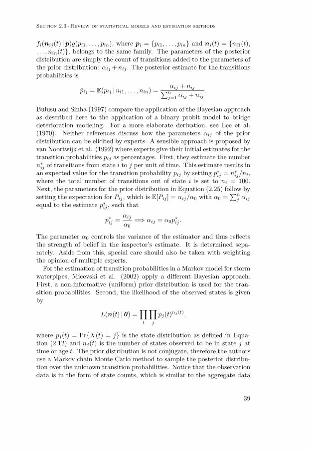
Section 2.3 ·Review of statistical models and estimation methods
39
fi(nij(t) |p)g(pi1, . . . , pin), where pi = {pi1, . . . , pin} and ni(t) = {ni1(t),. . . , nin(t)}, belongs to the same family. The parameters of the posteriordistribution are simply the count of transitions added to the parameters ofthe prior distribution: αij +nij . The posterior estimate for the transitionsprobabilities is
p̂ij = E(pij |ni1, . . . , nin) = αij + nij∑nj=1 αij + nij
.
Bulusu and Sinha (1997) compare the application of the Bayesian approachas described here to the application of a binary probit model to bridgedeterioration modeling. For a more elaborate derivation, see Lee et al.(1970). Neither references discuss how the parameters αij of the priordistribution can be elicited by experts. A sensible approach is proposed byvan Noortwijk et al. (1992) where experts give their initial estimates for thetransition probabilities pij as percentages. First, they estimate the numbern∗ij of transitions from state i to j per unit of time. This estimate results inan expected value for the transition probability pij by setting p∗ij = n∗ij/ni,where the total number of transitions out of state i is set to ni = 100.Next, the parameters for the prior distribution in Equation (2.25) follow bysetting the expectation for Pij , which is E[Pij ] = αij/α0 with α0 =
∑nj αij
equal to the estimate p∗ij , such that
p∗ij = αijα0
=⇒ αij = α0p∗ij .
The parameter α0 controls the variance of the estimator and thus reflectsthe strength of belief in the inspector’s estimate. It is determined sepa-rately. Aside from this, special care should also be taken with weightingthe opinion of multiple experts.
For the estimation of transition probabilities in a Markov model for stormwaterpipes, Micevski et al. (2002) apply a different Bayesian approach.First, a non-informative (uniform) prior distribution is used for the tran-sition probabilities. Second, the likelihood of the observed states is givenby
L(n(t) |θ) =∏t
∏j
pj(t)nj(t),
where pj(t) = Pr{X(t) = j} is the state distribution as defined in Equa-tion (2.12) and nj(t) is the number of states observed to be in state j attime or age t. The prior distribution is not conjugate, therefore the authorsuse a Markov chain Monte Carlo method to sample the posterior distribu-tion over the unknown transition probabilities. Notice that the observationdata is in the form of state counts, which is similar to the aggregate data

Chapter 2 ·Markov processes for bridge deterioration
40
used in the regression based models discussed in the section entitled “Re-gression using the state distribution” on page 27. This approach thereforesuffers from the same shortcoming that the observed states are treated asconditionally independent. There is no probabilistic link between two con-secutive inspections of a structure, even though this is the basic assumptionof the underlying Markov chain.
2.4 TESTING THE MARKOV PROPERTY
There exist statistical tests to verify if the Markov property holds for theobserved data. In general, all tests require full observations of the Markovprocesses and a sufficiently large number of observations to ensure accurateresults. Unfortunately, both requirements are often not met. This poses aproblem for the decision maker, who has assumed that the data is Markov-ian and wants to verify if his assumption is valid. For Markov chains whereeach transition is observed, there are a number of tests for the Markovproperty and for time dependence. One of the earliest references for thesetype of tests is Anderson and Goodman (1957). A more recent discussionin the context of economic analysis can be found in Bickenbach and Bode(2003).
A simplified test, equivalent to the tests described by Anderson andGoodman (1957), for the Markov property in bridge inspection data ispresented in Scherer and Glagola (1994). Basically, the authors test thestatistical significance of the difference between the probability of a se-quence of three states {i, j, k} and the probability of the sequence {j, k} byuse of a contingency table. Let
pijk = Pr{X(t3) = k |X(t2) = j,X(t1) = i}, (2.26)
then the Markov property assumes that p0jk = p1jk = p2jk = · · · = pjk.The number of observations for each sequence can be placed in a contin-gency table in order to calculate the value of the Chi-square test. Althoughnot all possible sequences could be tested (due to lack of data), those se-quences that were tested by Scherer and Glagola (1994) did not result ina rejection of the null hypothesis, which is the hypothesis that the (firstorder) Markov property holds.
Whether or not a test for the Markov property can effectively be per-formed largely dependends on the type of data which is available to thedecision maker. As explained in the introduction to this chapter, observedbridge condition states may be aggregated, which makes testing the Markovproperty practically impossible. In the Netherlands, bridges are inspectedthroughout the year and at different intervals, which results in panel data.Although the individual state histories are known to the decision maker,

Section 2.5 ·Using semi-Markov processes
41
the times between inspections may vary significantly. Therefore, it is pos-sible to count the number of sequences {i, j, k} in the data but the statesin this sequence may be observed at very different times. A simple countof sequences therefore ignores the fact that the observation times t1, t2 andt3 in Equation (2.26) are almost always different. This makes the validityof such tests questionable.
Unless the transitions of a Markov process are directly observed anda large number of observations are available, it must be concluded thattesting the hypothesis of the Markov property is not practically feasible.This conclusion was also drawn by Kay (1986), who proposed a possiblesolution using interpolation to recreate transition times, but conceded thatthis is a rudimentary workaround.
2.5 USING SEMI-MARKOV PROCESSES
Markov chains and continuous-time Markov processes are most often ap-plied due to their computational tractability. However, concerns are some-times raised about the constant transition intensity in each state. Becausedeterioration is at least partially or completely due to aging, some arguethat it would be appropriate for the model to include aging. The most com-mon probability distribution for the waiting time in each condition state,which enables the inclusion of aging, is the Weibull distribution. The cu-mulative distribution function for the Weibull distribution is given by
F (x) = 1− exp{−(λx)β} (2.27)
with scale parameter λ > 0 and shape parameter β > 0. The hazard rate,defined by
h(x) = f(x)1− F (x)
,
for the Weibull distribution is βλ(λx)β−1. If β = 1, then the hazardfunction is constant and the Weibull distribution reduces to the exponentialdistribution defined in Equation (2.5). If β > 1 the hazard rate is increasingand therefore the probability of a transition out of the current state in theimmediate future increases as the length of stay increases.
Although this approach may seem more appropriate from a physical pointof view, the absense of the memoryless property results in a model which isdifficult to work with. This is especially true when the deterioration processis not continuously monitored and only panel data is available. An exampleis the calculation of the time to failure in Kleiner (2001), which is given bya sum of Weibull distributions. As there is no analytical solution for thesum of Weibull distributed random variables, the author uses Monte Carlosimulation to obtain a numerical approximation. In the same paper, the

Chapter 2 ·Markov processes for bridge deterioration
42
author concedes that there is insufficient data to estimate the parametersof the waiting times and proposes that these be determined by expert judg-ment. Mishalani and Madanat (2002) suggest to use a maximum likelihoodapproach which takes into account left- and right-censoring in the waitingtime. However, their approach assumes that there are only two states andthat the time of (re)construction is known. Each inspection therefore re-sults in one of two possible observations: the transition has taken placebefore the inspection or it has not yet taken place. Another feature of theapproach in Mishalani and Madanat (2002) is that the Weibull distributedwaiting time is used to determine transition probabilities in a Markov chainwhich is necessarily nonstationary.
Another approach based on maximizing the likelihood of the observationsis presented by Black et al. (2005b) and compared to Markov chains and thedelay time model in Black et al. (2005a) using a case study. This approachis quite similar to the regression methods which use the state distribution aspreviously discussed in the section “Regression using the state distribution”on page 27, only now the waiting times are represented by Weibull randomvariables. This approach therefore suffers from the same shortcomings,like the fact that successive observations are essentially treated as beingindependent. An important assumption is that the construction year andthe initial state distribution are known, such that the probability of being inan observed state can be used to calculate the likelihood of the observations.The reason why there is a common perception that the probability of atransition should increase as the time spent in a state increases, is nicelyworded in Black et al. (2005a):
“If the condition states correspond to intervals of an underlyingcontinuous condition measure, then an item is likely to enter the statenear one boundary and then progress over the time periods to nearthe other boundary before leaving the state. Hence the transitionprobability is likely to increase as the item approaches the secondboundary, and so the transition probability could often increase withthe time spent in the state.”
As most classification schemes do not assume an underlying continuousprocess, like is illustrated with the quote on page 23, this reasoning is notrelevant in most cases.
SUMMARY
This chapter reviews the nature of bridge inspection data and various ap-proaches which have been suggested and applied to fit a finite-state Markovprocess to this data. Most statistical models ingnore the fundamental as-sumption of Markov processes; namely that the future states are indepen-dent of past states given the current state. These models use the state

Section 2.5 ·Using semi-Markov processes
43
observations as individual and independent observations, whereas thereshould be dependence between successive observations of the same struc-ture.
A better approach is to use the maximum likelihood principle, but thePoisson regression model on page 29 is too restrictive and the multinomialmodel on page 32 can only be used if the structure is continuously mon-itored. Other approaches, like a Bayesian approach or a nonparametricmodel, suffer from various shortcomings which make them unattractive fordecision makers.
Practically all bridge condition data, obtained using visual inspections,is in the form of panel data; that is, throughout the year inspections are pe-riodically performed at different intervals which results in a form of intervalcensoring. This heavily censored data can not be used to adequately testthe validity of the Markov assumption. However, the Markov assumptionis made by the decision maker in order to develop a tractable deteriora-tion model. Even if the underlying deterioration process does not possessthe Markov property, the assumption is necessary to be able to efficientlycalculate the outcome, which is required for decision making.


45
3Proposed framework
Given the conclusions drawn in the previous chapter on the various ap-proaches to fitting finite-state Markov processes to bridge condition data,this chapter describes the appoach selected for application to bridge con-dition data in the Netherlands. The likelihood function plays a centralrole in this approach and may be defined for perfect and imperfect inspec-tions. The calculation of the likelihood of the observed bridge conditionsinvolves the calculation of the transition probability function Pij(s, t) =Pr{X(t) = j |X(s) = i}, which gives the probability of a transition fromstate i to state j between ages s and t for s ≤ t. The calculation of Pij(s, t)is not straightforward, therefore several methods are presented separatelyin Chapter 7. Attention is also given to covariate analysis, which tests ifconsidering different groups of bridges will considerably influence the out-come of the model. Also, Section 3.4 lists the data requirements for thesuccessful application of this estimation procedure.
3.1 MAXIMUM LIKELIHOOD ESTIMATION
For a given set of data, the likelihood is defined as the probability thatthe chosen model generates the data. It is simply the joint density ofthe random variables of the model. For the purpose of estimation, thelikelihood is considered to be a function of the unknown model parameters(Mood et al., 1974, p.278).
Given the sample set x = {x1, x2, . . . , xn}, the likelihood that the setof parameters θ = {θ1, . . . , θm} generates the data is given by the like-lihood function L(θ;x). The notation (θ;x) means that it is a functionof θ given the data x, but that it is not a conditional probability. Obvi-ously, 0 ≤ L(θ;x) ≤ 1. The problem of estimation is now reduced to aproblem of maximizing the likelihood function; that is, to find those val-ues for the model parameters which maximize the likelihood function. Anequivalent problem arises when taking the natural logarithm of the likeli-hood function. The locations of the maxima of the log-likelihood function`(θ;x) = logL(θ;x) and the likelihood function L(θ;x) are the same. Itis generally easier to work with the logarithm of the likehood function asopposed to working with the likelihood function itself. This is especiallytrue if the observations of the model are considered to be independent. Let

Chapter 3 ·Proposed framework
46
fM (x) be the probability of taking a sample x from the model M , thenunder the assumption of independent sampling the log-likelihood functionis given by
`(θ;x) = log∏i
fM (xi) =∑i
log fM (xi) (3.1)
for samples xi, i = 1, 2, . . .. Here, the dependence of the model M on theset of parameters θ is surpressed; i.e., M ≡M(θ).
The use of maximum likelihood estimation for panel data is quite com-mon. The likelihood function as given by Equation (3.1) can readily befound in the literature. For example, it is common in publications in thefield of medical statistics: Jackson et al. (2003) provide an overview, whichincludes Kay (1986). The latter discusses the application of a continuous-time Markov process to the development of cancer markers over time.These markers are used to grade levels of disease in order to identify vari-ous states in the development of an illness. An important reference is thepaper by Kalbfleisch and Lawless (1985), which includes many of the top-ics discussed in this chapter and uses an example of a longitudinal studyof smoking habits of school children. Like many studies, the assessmentof smoking habits is done at infrequent moments in time at which a largegroup of subjects is evaluated at the same time. This results in paneldata and Kalbfleisch and Lawless (1985) used Fisher’s method of scoringin combination with the diagonalization method for calculating the tran-sition probability function (see page 115 in Chapter 7). The method ofscoring will be presented in Section 3.3.
Other than the fact that it is particularly well suited for applicationto panel data, maximum likelihood estimation has the additional ben-efit that, under suitable conditions and if the sample set is sufficientlylarge, the estimator is approximately Gaussian (i.e., normally distributed).According to a well known theorem (see e.g., Mood et al. (1974, The-orem 18 on page 359)) the estimator θ̂∗ of the true value θ∗ asymp-totically has an m-dimensional multivariate normal distribution: θ̂∗ ∼MVNm(θ∗, Ie(θ∗)−1)/n. Here, Ie(θ) is the expected information matrix,which will be discussed in the next section.
The concept of maximum likelihood estimation was developed in theearly 20th century by British statistician R.A. Fisher (1912 and 1922) and isnow a common method for statistical inference. In the following section, thelikelihood functions for both perfect and imperfect periodic observations ofa finite-state Markov process are derived.

Section 3.2 · Statistical model
47
3.2 STATISTICAL MODEL
As the model under consideration is a stochastic process, an observation ofthe model M is a collection or sequence of one or more state observationsat successive times t1 < t2 < · · · < tn. The process starts at t0 = 0 and itis assumed here that the initial state X(t0) is known to the decision maker.For ease of notation, Xk ≡ X(tk) is used in the following discussion.
3.2.1 LIKELIHOOD FUNCTION FOR PERFECT OBSERVATIONS
The likelihood function for perfect observations is quite straightforward.With ‘perfect’, it is meant that no error is made in the assessment of thetrue condition state of the structure or component. For each object, a se-quence {X1, X2, . . . , Xn} of state observations is available. The probabilityof each sequence may conveniently be written as a product of transitionprobability functions:
Pr{X1, X2, . . . , Xn} = Pr{X0}n∏k=0
Pr{Xk+1 |Xk}, (3.2)
where the probability distribution of the initial condition state Pr{X0} isassumed to be known.
Special attention should be given to the case where an observed transitionis not possible given the model. In this case, Pr{Xk+1 |Xk} = 0 andtaking the logarithm will result in an error. This situation can arise if onlydeterioration is allowed, but an improvement in the condition is observed.These cases should simply be discarded by the implementation. Thereare two options for how to deal with these cases: discard the impossibletransition or discard the complete sequence of observations of which thetransition is a part. In order to use as much data as possible, the firstoption is preferred. However, this may be subject to debate because it mayseem more natural to choose for the second option. In the next section,a model which allows for imperfect inspections will be presented and thealgorithm used in this model discards the complete sequence of observedbridge conditions.
3.2.2 LIKELIHOOD FUNCTION FOR IMPERFECT OBSERVATIONS
In order to model the subjectiveness of visual inspections and the naturalvariability which arises from this, it is possible to consider that inspectionsmay not accurately describe the true state of the process. By ‘imperfect’it is meant that there exists a true state and that, with some probabil-ity, an inspection may indicate a different state other than the true state.Other suitable designations for this topic include ‘inspection accuracy’ or

Chapter 3 ·Proposed framework
48
5 5
5 5
X0 X1
Y1
X2
Y2
. . . Xn
Yn
P (t0, t1)
Pr{Y1 |X1}
P (t1, t2)
Pr{Y2 |X2} Pr{Yn |Xn}
Figure 3.1: Graphical representation of ahidden Markov model.
‘inspection variability’. It is noted that an inspector can never be blamedfor making ‘inaccurate’ observations, as he or she is required to give apersonal assessment which, in his or her view, best reflects the conditionstate.
This subject has been of great interest in the past and with good reason.It is obvious that the personal interpretation of condition states, like thosein Tables 1.1 and 2.1, and how these relate to damages on structures willvary substantially between inspectors. A study by Phares et al. (2002)has shown that there is indeed a substantial difference between the ratingsfrom different inspectors. This variability may also account for some ofthe increases in the quality of structures which can not be attributed tomaintenance. In general, data sets from inspections will include transitionstowards better conditions, which can not be eliminated on the basis of beinga result of maintenance. Since a monotonically increasing Markov processfor modeling deterioration can not cope with condition improvements, thesepose a challenge for the decision maker. In various studies, such as thoseconducted by Kallen and van Noortwijk (2005b) and Morcous (2006), thecondition improvements are simply removed from the data.
A modeling approach for incorporating imperfect inspections and whichis commonly applied to problems in speech recognition, is the use of ahidden Markov model. Although visual inspections are the only meansby which the state of deterioration may be measured, the hidden Markovapproach assumes that there is some true condition state which is ‘hidden’to the observer. Figure 3.1 shows a graphical representation of the hiddenMarkov model.
In this figure, the true states X1, X2, . . . , Xn at the inspection timest1, t2, . . . , tn are hidden behind the actual observed states Y1, Y2, . . . , Yn.The probability of the observations, given the true state, is given by eij =Pr{Yk = j |Xk = i}, where 0 ≤ eij ≤ 1 and
∑j eij = 1. The (discrete)
probability distribution ei = {ei1, . . . , ein} reflects the variability in theinspections. These ‘error’ distributions can be assessed by expert judg-ment, testing a pool of experts using selected test cases, or by maximum

Section 3.2 · Statistical model
49
likelihood. The decision maker must also choose how large the inspectors’mistakes are allowed to be. He may restrict the model such that only anerror of one state (higher or lower) can be made.
The observed sequence Y1, Y2, . . . , Yn has several properties, but it doesnot possess the Markov property. One of the primary problems involvedwith the use of hidden Markov models, is determining the probability ofthe observed sequence given the model. This probability is required formaximum likelihood estimation. Most properties rely on the basic propertythat, conditional on the true process, the observations Yk for k = 1, . . . , n,are independent; that is:
Pr{Y1, . . . , Yn |X1, . . . Xn} =n∏k=1
Pr{Yk |Xk}.
The probability of the observed sequence may be determined by
Pr{Y } =∑∀X
Pr{Y ,X} =∑∀X
Pr{Y |X}Pr{X}, (3.3)
where Y = {Y1, . . . , Yn} andX = {X1, . . . , Xn}. The summation in Equa-tion (3.3) is taken over all possible sequences X. As this approach is com-putationally very inefficient, there exists the ‘forward-backward’ algorithm.The forward part of this algorithm is most frequently used to calculate thelikelihood of the observed sequence. Let the forward variable be defined as
α(k)i = Pr{Y1, Y2, . . . , Yk, Xk = i},
which is the probability of the observations up to time tk and the true stateat time tk being equal to i. The forward algorithm starts with k = 1:
α(1)i = Pr{Y1, X1 = i |X0} = Pr{Y1 |X1 = i}Pr{X1 = i |X0}
and continues for k > 1 using the relation
α(k+1)i = Pr{Yk+1 |Xk+1 = i}
∑j
α(k)j Pr{Xk+1 = i |Xk = j} (3.4)
up to α(n)i . The likelihood of the complete sequence of observations may
then be obtained by summing over all Xn:
Pr{Y1, . . . , Yn} =∑i
α(n)i .
This approach is also referred to as the Baum-Welch algorithm. The prop-erties of hidden Markov models, on which this algorithm relies, are dis-cussed and proven in MacDonald and Zucchini (1997).

Chapter 3 ·Proposed framework
50
Note that this algorithm will set the likelihood of the complete conditionhistory of a structure to zero if one of the transitions is not possible withthe given model. This can be observed in Equation (3.4):
if α(k)i = 0 for all i, then
∑i
α(n)i = 0 for n ≥ k.
In order to check the correctness of the implementation of this model,one can take the probability of a misclassification to be zero and comparethe results of the model with those obtained from the model with perfectinspections. For this, one should set eii = 1 and eij = 0 for i 6= j and letthe model for perfect inspections discard complete observation sequences ifone of the transitions in the sequence is not possible. Also, the probabilityof the first observed condition must be one, i.e. Pr{Y1 = y1} = 1 for theobserved state y1.
Some other approaches to this problem can be found in the literature.For example, Jackson et al. (2003) formulate Equation (3.3) as a productof matrices, which is just the forward-backward algorithm in matrix for-mulation; see also MacDonald and Zucchini (1997, p.61). In Cappé et al.(1998), the likelihood of the observed sequence is rewritten as
Pr{Y1, . . . , Yn} =n∏k=1
Pr{Yk |Y1, . . . , Yk−1}
=n∏k=1
∑j
Pr{Yk, Xk = j |Y1, . . . , Yk−1}
=n∏k=1
∑j
Pr{Yk |Xk = j}Pr{Xk = j |Y1, . . . , Yk−1}.
Using the logarithm of this result, they propose a recursive algorithm whichalso enables the calculation of the derivatives with respect to the modelparameters iteratively.
The name ‘hidden’ is primarily used in the area of speech recognition,where Rabiner (1989) is often cited. In the field of operations research, thesame model is referred to as a ‘partially observable’ Markov model. Thelatter has been applied to the problem of bridge management by Ellis etal. (1995), Jiang et al. (2000) and Corotis et al. (2005). The same modelhas also been referred to as a ‘latent’ Markov model and applied to bridgemanagement by Madanat (1993) and Smilowitz and Madanat (2000). In allof these publications, the use of a hidden Markov model is combined witha Markov decision process (see the section on Markov decision processeson page 87).

Section 3.2 · Statistical model
51
3.2.3 COVARIATE ANALYSIS
Covariate analysis is often used in the field of survival analysis and aimsto determine which ‘covariates’ influence the outcome of the model. Co-variates are simply additional variables, also called ‘independent’ variables,which take on two or more values depending on the properties of a structure.In medical applications, a very common covariate is the sex of patients. Asan example, let Xs represent this covariate and let Xs = 0 if the patient isa male and Xs = 1 if the patient is a female. In essence, covariate analysisgroups the objects according to one of their properties and then assessesthe impact of this grouping on the estimate of the parameters. If, in theexample of the patients, the outcome is significantly different, it must beconcluded that a patient’s sex is a statistically significant variable in themodel. Using a mathematical formulation: suppose one wants to estimatethe transition intensity λ > 0 in a continuous-time Markov processes, thenthe covariate model looks like
λs = exp{β0 + β1Xs}, (3.5)
where β0 is the intercept and β1 is the coefficient of the variable Xs. Usingthis reparametrization, the ‘new’ parameters β = {β0, β1} are estimated.The model in Equation (3.5) is referred to as a multiplicative model, whereexp{β0} represents the ‘base rate’ and exp{β1Xs} is the adjustment dueto Xs. If β1 turns out to be close to zero, such that the adjustment isclose to unity, it may be concluded that grouping of patients according totheir sex does not influence the outcome of the estimation. A formal testlike a likelihood ratio hypothesis test may be used to validate or reject thehypothesis that a covariate is not statistically significant.
In Skuriat-Olechnowska (2005), a simple Wald test was used for thepurpose of testing the statistical influence of each covariate in the analysis.Using the fact that the maximum likelihood estimator for each coefficientβk, k = 0, 1, 2, . . . , is asymptotically normal, the Wald test defines theZ-statistic as the ratio
Zk = β̂k − βkSEβ̂k
,
where SEβ̂k is the standard error of the estimator β̂k. The standard error isthe estimated standard deviation of the estimator. The null hypothesis isthat the covariate i does not significantly influence the transition intensities.In other words: that the coefficient βk is not significantly different fromzero. The hypothesis βk = 0 is rejected if the two-sided p-value Pr{|Zk| >β̂k/SEβ̂k} is small. Basically, the Wald test rejects the hypothesis at (for

Chapter 3 ·Proposed framework
52
example) the 5% significance level if zero is not inside the 95% confidencebounds of the estimated coefficient βk.
The log-linear model λ = exp{βX}, with X = {1, X1, X2, . . . , Xn} is aconvenient model, because the positive exponential function ensures thatthe requirement λ > 0 always holds. For discrete-time Markov processes,the transition probabilities p may be reparametrized as
p =(1 + exp{−βX}
)−1, (3.6)
such that 0 ≤ p ≤ 1. Both approaches are particularly well suited for usein a maximization procedure, which is the topic of the next section.
3.3 MAXIMIZATION
In most practical cases, it is infeasible to analytically maximize the log-likelihood function, therefore a numerical approach is used. Concepts likeNewton’s method, quasi-Newton methods, and Fisher’s method of scor-ing are introduced in this section. Fisher’s method of scoring is a quasi-Newton method specifically used for maximizing likelihood functions andquasi-Newton methods are approximations to Newton’s method, which isan iterative approximation scheme with reasonably fast (quadratic) con-vergence to the root of a differentiable function.
Newton’s method
Newton’s method (also referred to as Newton-Raphson) is a root-findingalgorithm for (systems of) non-linear and continuously differentiable func-tions. For a vector x = {x1, x2, . . . , xn} and f : Rn → R a differentiablefunction, the algorithm attempts to iteratively approximate a root x∗ forwhich f(x∗) = 0. The method is based on a Taylor series expansion of thefunction f(x) around a value a: f(x) = (x− a)f ′(x), or if solved towardsa: a = x − f(x)/f ′(x). If a = x, then f(x) = 0 and the aim of New-ton’s method is to approximate the unknown x∗ with iterative adjustmentsto a. This is done by taking an initial guess x0 for x∗ and successivelycalculating x1,x2, . . . using the relation
xk+1 = xk −f(xk)f ′(xk)
, (3.7)
for k = 0, 1, 2, . . . until ‖ xk+1−xk ‖< ε. This algorithm is not guaranteedto converge, but it converges fairly fast when it does converge. If there aremultiple (local) extremes in the function f , then the algorithm is also notguaranteed to converge to the global extreme.
The algorithm can also be used for a system of non-linear equations. Letf(x) = {f1(x), f2(x), . . . , fm(x)}, then Equation (3.7) becomes

Section 3.3 ·Maximization
53
xk+1 = xk − J−1(x)f(xk), (3.8)
where J−1(x) is the inverse Jacobian of f(x). For the system of equationsf(x), the Jacobian is the n×m matrix defined as
J =
∂f1∂x1
∂f2∂x1
. . . ∂fm∂x1
∂f1∂x2
∂f2∂x2
. . . ∂fm∂x2
......
. . ....
∂f1∂xn
∂f2∂xn
. . . ∂fm∂xn
.The location of the extremes of a function f(x) may be determined bysetting the partial derivatives to each of the variables xi equal to zero andsolving for xi. For x ∈ Rn, this results in the requirement to solve a systemof n (non-linear) equations:
∂f
∂x1= 0, ∂f∂x2
= 0, . . . , ∂f∂xn
= 0.
Let
f ′(x) =
{∂f
∂x1,∂f
∂x2, . . . ,
∂f
∂xn
},
then Newton’s step for iteratively approximating x∗, such that f(x∗) = 0,becomes
xk+1 = xk −H−1(xk)f ′(xk) (3.9)
for k = 0, 1, 2, . . . . Here, H−1(x) is the inverse Hessian matrix of f(x)defined as
H =
∂2f∂x2
1
∂2f∂x1∂x2
. . . ∂2f∂x1∂xn
∂2f∂x2∂x1
∂2f∂x2
2. . . ∂2f
∂x2∂xn
......
. . ....
∂2f∂xn∂x1
∂2f∂xn∂x2
. . . ∂2f∂x2n
.
If f(x) is a log-likelihood function, then f ′(x) and −H(x) are referred toas the score function (or efficient score) and the information respectively.In this context, define
sθi = ∂
∂θi`(θ;x),
and in vector notation:

Chapter 3 ·Proposed framework
54
s = ∂∂θ`(θ;x)
as the score function. The information is denoted by Io(θ;x) = −∂s/∂θ =−H(x). The dependence of s and H on θ is suppressed in the notation.
Note that Newton’s method is a method for unconstrained optimization,which means that the parameters of the function to be minimized are notconstrained. As most practical applications have some restrictions on thedomain of the parameters, a reparametrization is used. For continuous-time or discrete-time Markov processes, Equations (3.5) and (3.6) may beused respectively.
Quasi-Newton methods and Fisher’s method of scoring
The adjustment in Equation (3.7) and Equation (3.8) contains the firstderivative of the function f with respect to each parameter and the Newtonstep in Equation (3.9) also requires the second derivatives. In most cases,these derivatives are not easily obtained, therefore they are replaced byapproximations which do not require the derivatives themselves. Whenusing this approach, Newton’s method is commonly referred to as a quasi-Newton method.
Fisher proposed to replace the information with the expected value (overall possible realizations of the model) denoted by Ie(θ;x) = E[I]. Thisapproach eliminates the need to calculate the second derivatives of thelikelihood function. This can be shown as follows: let f(x;θ) = L(θ;x)and `(θ;x) = log f(x;θ), then
Iθiθj = − ∂∂θj
[1f
∂f
∂θi
]= −[− 1f2∂f
∂θj
∂f
∂θi+ 1f
∂2f
∂θj∂θi
]= sθjsθi −
1f
∂2f
∂θj∂θi.
Multiplying each side with the density f(x;θ) and integrating over allpossible values of x results in∫
x
Ioθiθjfdx =∫x
sθjsθifdx−∫x
∂2f
∂θj∂θidx.
As ∫x
∂2f
∂θj∂θi= ∂2
∂θj∂θi
∫x
fdx = 0,
Section 3.4 ·Data requirements for model application
55
this reduces to E[Iθiθj]
= E[sθjsθi
]. Because it is generally not feasible
to calculate the expected information, the ‘observed’ information Ioθiθj isdetermined instead. The observed information is approximation of the ex-pectation by the mean over the observed data. For multiple (independent)observations of the model, the score and information become
sθi(θ;x) = ∂
∂θilog∏∀k
fM(θ)(xk) =∑∀k
∂
∂θilog fM(θ)(xk) =
∑∀k
sθi(θ;xk)
and
Io(θ;x) = − ∂2
∂θi∂θjlog∏∀k
fM (xk;θ) =∑∀k
− ∂2
∂θi∂θjlog fM (xk;θ)
=∑∀k
Io(θ;xk)
respectively. Therefore, the total score and information are simply the sumof the individual scores and informations.
3.4 DATA REQUIREMENTS FOR MODEL APPLICATION
There are several requirements which have to be met if bridge inspectiondata is to be used in a maximum likelihood estimation procedure as de-scribed in this chapter. First, there have to be a minimum number ofinspections available for each structure if it is to contribute to the likeli-hood function. For a model with perfect inspections, these should be
− at least two successive state observations if the bridge was constructedbefore registration of inspection results was initiated,
− and at least one if the bridge was constructed after registration of in-spection results was initiated.
If inspections are assumed to be imperfect, the requirements are that
− there is at least one state observation available if the bridge was con-structed before registration of inspection results was initiated and thatan assumption be made about the actual state distribution at the timeof the first inspection,
− and there is at least one state observation available if the bridge wasconstructed after registration of inspection results was initiated and theinitial state distribution at service start of the bridge is given.
The assumption about the distribution of the actual state at the first in-spection, is required due to the fact that there is no information about the

Chapter 3 ·Proposed framework
56
state at the service start of the structure or on past maintenance activi-ties. The distribution of X1 conditional on X0 is therefore not availableand should be replaced by a distribution over X1 selected by the decisionmaker. There is no exact rule for the minimum number of state histories(i.e., structures available for the analysis) which must be available for a suc-cessful application of maximum likelihood estimation. A simple guidelineis: the more, the better.
SUMMARY
This chapter presents the theoretical foundation for the maximum like-lihood estimation of transition intensities in a continuous-time Markovprocess. The maximum likelihood approach is particularly well suited forpanel data, because it considers the likelihood of the periodic state obser-vations and it uses the transition probabilities to determine this likelihood.The method therefore respects the Markov assumption and it does not relyon information which is not available, namely information on the exacttimes of transitions or the exact length of stay in any state. For the ap-plication of this method, the data must fulfill certain requirements, whichare outlined in the previous section.
The likelihood function can be defined to achieve several goals: estimatethe model parameters under the assumption that state observations areperfect (Section 3.2.1) or imperfect (Section 3.2.2), or to determine theinfluence of dependent variables in a covariate analysis (Section 3.2.3). Thelikelihood must then be maximized as a function of the model parameters,such that the parameter values are the most likely ones to have generatedthe given data. The most common method for maximizing the likelihoodfunction is Fisher’s method of scoring, which is discussed in Section 3.3.

57
4Application and results
In this chapter, the approach proposed in Chapter 3 will be applied tobridge condition data obtained in the Netherlands. A general introductionto the practice of inspecting bridges in the Netherlands was given in Sec-tion 1.3 on page 6. The most important aspect of bridge inspections isthat individual damages are registered in the database and that the sever-ity of these damages is then used to set the condition of the structure. Theseverity of the damages is also used to set the condition of the basic andprimary components on which the damages are located.
First, a description of the available data sets will be given. Then, variousmodels with different transition structures are fitted to the data sets. InSection 4.2.1, this is done for progressive Markov processes which only allowfor deterioration, and in Section 4.2.2, this is done for models which alsoallow for transitions to better states. Sections 4.3 and 4.4 respectively dis-cuss the application of hidden Markov models and the analysis of covariateinfluences on the model parameters.
4.1 DUTCH BRIDGE CONDITION DATA
In the Netherlands, bridge inspections register the location and severity ofall damages present on the structure. These severities are then used bythe database and by the inspector to set the condition of the individualcomponents and the overall condition of the structure. In order to succes-fully fit a deterioration model, it is necessary to have a sufficient amountof data. This is especially true for fitting stocastic processes for modelinguncertain deterioration over time.
4.1.1 QUALITY AND DETAIL OF INFORMATION
Although it is not mandatory, the cause of each damage may be registeredin the database. From a decision maker’s point of view, it may be inter-esting to identify different physical deterioration mechanisms and to fit thedeterioration model to the historic development of the damages. However,it is not possible to identify the same damages between successive inspec-tions in the database. This is because the identification of the location ofeach damage is done by issuing a location number on a technical drawing

Chapter 4 ·Application and results
58
of the structure. Inspectors issue these locations anew at each inspection,therefore the same damage may have a different location number at differ-ent inspections. From a practical point of view, it is not feasible to visuallycheck the location of damages for all inspections in the database. Afterfiltering for incorrect or incomplete entries, there are roughly 6000 inspec-tion events on 2300 structures which can be used for modeling deteriorationwith Markov processes.
There are various reasons why some inspection events or structures maynot be included in the data sets.
− A structure may not have a construction year assigned to it, which isnecessary information for determining the age of structures at the timeof an inspection. The construction year may also be faulty; for example,it may be after 2004 which is the last year in which inspections wereregistered in the database.
− An inspection event may have an incorrect date assigned to it, wherethe year of the inspection is before the construction year of the structureor after 2004.
− A structure may not have undergone enough inspections. In general,structures should at least have been inspected twice, such that tworeference points in time are available. For structures built after 1985only one inspection is required, because the initial state (i.e., perfector state ‘0’, see Table 1.1) can be used as the first ‘observation’. Forbridges constructed before 1985, it is not known if maintenance wasperformed before the registration in the database began.
It is a not an easy task to extract the data from the relational database andputting this information in a form suitable for estimating the model pa-rameters. Aside from the easily identifiable faulty data mentioned above,there are an unknown number of entries in the database which are alsofaulty, but which can not easily be identified as such. One such exam-ple occurs when an inspector incorrectly registers a condition 0, when thepurpose of the inspection was not to assess the condition of the structure.Some inspections are performed to investigate specific areas or damageson the structure. These inspections should be registered, but no condi-tion number should be entered into the database. The analysis of textualremarks in the database may be able to filter out these entries, but thisrequires a significant amount of work.
Another area where mistakes can enter the database is in the dates ofinspections. The date which is registered in the database may not actuallybe the date at which the inspection physically took place. The durationsbetween the inspection dates in the database are collected in a histogramin Figure 4.1. Even though inspections are performed periodically, there’squite a bit of variability in the actual times between these inspections. This

Section 4.1 ·Dutch bridge condition data
59
11 11
11 11
0–1
1–2
2–3
3–4
4–5 5–
66–
77–
8 8–9
9–10
10-11
11-12
12–1
313
–1414
–1515
–1616
–17
0%
4%
8%
12%
16%
Figure 4.1: Histogram of the number ofyears between bridge inspections in theNetherlands.
is mainly due to the actual planning and execution of inspections resultingin different inspection intervals. Some of the differences will also be due tothe fact that the date in the database does not always correspond to theactual date of the inspection.
All the anomalies mentioned up to now are the result of inconsistentor erroneous behaviour by the inspectors. There is however another typeof faulty data: the absence of information on when maintenance was per-formed on the structure. When faced with an increase in the conditionof a structure, the decision maker would like to attribute this increase toeither maintenance or to a difference of opinion between two inspectors.Although the condition database in the Netherlands has the capabilityto register maintenance activities, this feature has seldomly been used.Morcous (2006) reports the same lack of maintenance data in the bridgecondition data for Québec in Canada.
From this discussion, one may conclude that the quality of the data isinsufficient for use in maintenance management. However, some of the in-consistencies are the inevitable result of the long duration of 20 years ofoperating the database and of the many people involved in the inspections.Even after filtering for faulty data, the number of observed bridge condi-tions is very large and is certainly suitable for use in a statistical analysis.
As mentioned in Section 1.3 of the introduction, the inspections do notlead to a uniform observation of all condition states. The histogram in

Chapter 4 ·Application and results
60
12 12
12 12
0 1 2 3 4 5 60%
10%
20%
30%
40%
Figure 4.2: Histogram of the observedstates in the bridge condition database in theNetherlands.
Figure 4.2 shows that states 4, 5 and 6 of the condition scale in Table 1.1are observed much less often than states 0 to 3. Because the last state,namely state 6, is extremely rare, it has been combined with state 5 toform a new state representing the conditions ‘bad’ and worse. The numberof states considered in this chapter, is therefore equal to six.
4.1.2 EXTRACTION FROM DATABASE
The original database is a relational database, which means that the in-formation is stored in various tables which are related to eachother. Thetables containing the basic information on the structures (e.g., name, lo-cation, size, etc.) are relatively static as changes in this information arenot frequent. The information obtained through inspections constitutesthe more dynamic part of the database. For each inspection, an entry ismade in a table and each entry is linked to the relevant structure in anothertable. This allows information to be added efficiently and in a structuredmanner.
For the purpose of a statistical analysis, the relational database is notthe most convenient form for data storage. Therefore the data is extractedfrom the database and stored in a spreadsheet. For each inspection, a newline containing all necessary information for the analysis is written to thespreadsheet. This includes at least a unique identifier, the year of construc-tion, the inspection date and the condition state. Other information, for

Section 4.1 ·Dutch bridge condition data
61
example for use in a covariate analysis, may also be included. The finalstep in the extraction process, is to prepare the data for use in a programfor numerical analysis. For maximum portability, the data is written toa plain text file. There are two options for this: 1) each line contains atransition, or 2) each line contains only an observation. The first optionresults in a file of the form
1 249 341 1 32 213 306 1 33 213 309 1 2...17 248 261 1 217 261 351 2 3...
Here, the first column includes a unique identifier. The second and thirdcolumns contain the age in months at two consecutive inspections and thefourth and last columns contain the condition states at these inspections.The second option contains the same data in a different form:
1 249 11 341 32 213 12 306 33 213 13 309 2...17 248 117 261 217 351 3...
Each observation is on a different line, where the first column includesthe identifier, the second the age in months at the inspection, and the thirdthe observed state.
The first option can be used for estimating the parameters of the Markovprocess when inspections are assumed to be perfect. The second option isparticularly well suited for applications where inspections may vary, butcan equally well be used for models with perfect inspections.
4.1.3 DESCRIPTION OF DATA SETS
In this chapter, four data sets will be used: general condition of structures,most severe damage condition of structure, superstructure conditions, andthe condition of kerbs. Each of these are briefly explained here.

Chapter 4 ·Application and results
62
General condition of structures
The general or overall condition of the structure is the condition statewhich is assigned to the ‘logical structure’ in the database as shown inFigure 1.5. This data set, and the one described next, contains the mostobservations of all data sets. As mentioned earlier, the condition dataassigned to a structure and its components is derived from the severity ofdamages registered at each inspection. Therefore, the components will notbe assigned a condition state at each inspection, unless there are one ormore damages present on the component.
Most severe damage on structures
The general condition of a structure is automatically assigned the mostsevere condition of the damages present at the time of an inspection. Theinspector must manually change this condition if it is not representativefor the structure as a whole. As a sort of ‘worst case scenario’, the analysisis also performed on a data set which includes the condition indicators ofthe most severe damages registered at each inspection.
Condition of superstructures
The superstructure of a bridge is generally considered to be all structureabove the bearings. This includes the beams, road surface, kerbs, and safetybarriers. In Figure 1.5, superstructures belong to the group of principalcomponents. This data set includes roughly 5500 observations.
Condition of kerbs
Kerbs (or curbs) are the rims along the roadway, forming an edge for asidewalk or for the safety barriers. There are roughly 5500 observations ofkerb condition states.
4.2 SELECTION OF TRANSITION STRUCTURE
Finite-state Markov processes are completely shaped by the transitionstructure defined in the transition intensity matrix. This matrix deter-mines when and to where a transition can take place. Before embarking onfitting a Markov deterioration process to observed condition data, the de-cision maker must decide how deterioration may procede. It is possible tochoose a fully filled transition matrix, which allows for transitions betweenany two condition states including transitions to better states. This, how-ever, will generally not be a very useful approach. In this section, various‘models’ will be fitted to the Dutch bridge condition data. These modelsare distinguished by the absence (without maintenance) or presence (withmaintenance) of backward transitions.

Section 4.2 · Selection of transition structure
63
4.2.1 MODELS WITHOUT MAINTENANCE
This section discusses the estimation of transition intensities in sequentialMarkov deterioration processes. Structures are therefore only allowed tomove to the next state and not move backwards to better states. The basictransition intensity matrix is then given by
Q(t) =
−λ0(t) λ0(t) 0 0 0 0
0 −λ1(t) λ1(t) 0 0 00 0 −λ2(t) λ2(t) 0 00 0 0 −λ3(t) λ3(t) 00 0 0 0 −λ4(t) λ4(t)0 0 0 0 0 0
. (4.1)
An unlimited number of choices are available for the elements λi(t), i =0, . . . , 4, but only five options will be considered here. These options aredefined in Table 4.1.
Model λi(t) n Description
A a 1 state- and age-independentB abtb−1 2 state-independent and age-dependentC ai 5 state-dependent and age-independentD aibt
b−1 6 state- and age-dependentE aibit
bi−1 10 state- and age-dependent
where a, ai, t > 0 and −∞ < b, bi <∞ for i = 0, . . . , 4
Table 4.1: Five options for the transitionintensity parameters in a sequential Markovdeterioration process.
This table names the models A to E according to the number of parametersn included in the model. Model A has only one parameter, whereas modelE has ten parameters. These roughly correspond to the models presentedin Kallen and van Noortwijk (2006b), only model D has been renamed to Eand an extra model with six parameters has been introduced as model D.Both models are state- and age-dependent, but compared to model E, thedependence on age is not state dependent as in model D. For model D, theage-dependent transition intensity matrix may be written asQ(t) = Qf(t),where f(t) = tb−1. In other words, the intensity matrix may be decomposedin an age-constant matrix and a scalar function which changes the intensityof the transitions over the age of structures if b 6= 1. The choice for thetransition intensity function is arbitrary and λ(t) = abtb−1 is chosen hereto obtain a power law function for the integrated intensity function: Λ(t) =atb.

Chapter 4 ·Application and results
64
Using the maximum likelihood framework as proposed in Chapter 3, thefive models in Table 4.1 will be fitted to the available data sets. Note thatthese are nested models, with model E being the most general formulation,such that their relative quality of fit may be compared using standardstatistical methods.
Overall bridge conditions
First, all models in Table 4.1 will be fitted to the observed overall conditionstates for the structures. Then the relative quality of fit will be comparedsuch that a verdict can be made as to which model is most suitable forthe data at hand. Note that the estimates for the parameters and thecorresponding log-likelihood values are similar, but different from thosereported in Kallen and van Noortwijk (2006b). This is because the dataset used to obtain the results in the paper contained quite a few duplicateentries.
i Model A Model B Model C Model D Model Eai bi ai bi ai bi ai bi ai bi
0 0.18 1 1.44 0.66 0.61 1 0.48 1.06 1.19 0.851 0.18 1 1.44 0.66 0.40 1 0.29 1.06 0.10 1.242 0.18 1 1.44 0.66 0.12 1 0.08 1.06 0.10 1.043 0.18 1 1.44 0.66 0.04 1 0.02 1.06 0.17 0.774 0.18 1 1.44 0.66 0.12 1 0.08 1.06 0.32 0.86
Table 4.2: Estimated parameter values forthe models without maintenance, where theunit of time is 1 year.
The results of the maximum likelihood estimation for models A to E arepresented in Table 4.2. Even with an ever evolving set of data, the resultfor, for example, model A is close to the result reported in Kallen and vanNoortwijk (2005b). The estimated annual transition intensity is 0.18, suchthat the mean waiting time in each state is approximately 5.5 years. Thebest estimate for the parameters in model B, where the transition ratesalso depend on the age of the structure, results in a decreasing intensityrate as the structures increase in age. Model C, with state-dependenttransition rates, shows decreasing rates as the condition worsens. The samecan be seen with model D, but with lower rates which increase slightlywith increasing age. Model E, with state- and age-dependent transitionintensities shows a mixed picture. The decreasing transition intensity inmodel B can be explained by the fact that bridges spend less time in initialstates compared to later states, which can be seen in the parameters ofmodel C in Table 4.2. Since there is a positive correlation between the

Section 4.2 · Selection of transition structure
65
bridge age [yr]
den
sity
[−
]
0 20 40 60 80 100 120 140 160
0.00
0.01
0.02
0.03
0.04
Model AModel BModel CModel DModel E
Figure 4.3: The probability density of thetime to reach the final state for the modelswithout maintenance.
age and state of a bridge, bridges have a higher transition intensity in theearlier stages of life.
Using the results in Table 4.2, it is possible to determine the time requiredto reach the last state, namely state 5, when starting from the initial state,namely state 0. The uncertainty in this time is represented by the ‘lifetime’distributions in Figure 4.3.
Because state 5 is not considered to be a failure state, these randomtimes do not represent true lifetime distributions. Therefore, they shouldnot be compared to the Weibull lifetimes estimated by van Noortwijk andKlatter (2004). State 5 should be considered as an undesirable conditionstate and a structure in this state should be attended to within a shortperiod of time. The mean time to reach state 5 and the 90% confidencebounds (represented by the 5% and the 90% percentiles) for the five modelsare listed in Table 4.3.
From this table and the results in Figure 4.3 it can be concluded thatthe models can be roughly grouped in two categories: models without statedependence (A and B) and models with state-dependence (C, D and E).The models without state dependence result in a much more narrow distri-bution compared to those with state-dependence. The difference betweenthe times to reach state 5 for models C, D and E, which have differentwaiting time distributions for each state, is very small. The mean time toreach state 5 for these three models is between 45 and 50 years, which isroughly halfway the design life of 80 to 100 years for bridges in the Nether-lands. If state 5 corresponds to a condition level where major renovation

Chapter 4 ·Application and results
66
Model 5% Mean 95%[yr] [yr] [yr]
A 11 28 50B 6 25 57C 14 45 96D 16 49 107E 14 50 126
Table 4.3: Mean value and the 5% and 95%percentiles of the time (in years) to reachthe final state for the models without main-tenance.
bridge age [yr]
condit
ion s
tate
[−
]
0 20 40 60 80 100 120 140 160
54
32
10
Model AModel BModel CModel DModel E
Figure 4.4: The expected condition stateas a function of age for the models withoutmaintenance.
is required, then this result is very much in line with current experience inthe Netherlands. A rule of thumb in the Netherlands is that bridges requiremajor repairs or renovation around 40 years of age. A noticable differencebetween models C, D and E is the increasing uncertainty towards higherages represented by an increasingly longer tail in the distribution.
Another interesting result is the expected condition state over time aspredicted by the Markov deterioration model. The same grouping accord-ing to state-dependence or -independence is observed in the expectationof the deterioration as is shown in Figure 4.4. All models converge tostate 5, which is an absorbing state in all five models. The linearity of theexpectation for model A in the initial states can clearly be observed.

Section 4.2 · Selection of transition structure
67
Relative quality of fit
The likelihood value of the data given a model, is an indicator for thequality of fit relative to the likelihood values of the other models. Thelarger the likelihood value of the model, the larger the probability thatthe data could be generated by the model. The same holds for the log-likelihood values. As can be observed in Table 4.4, the quality of the fitincreases with the number of parameters in the model.
Model Parameters log-likelihood BIC (−2/n)BIC
E 10 −3645 −3685 2.3503D 6 −3671 −3695 2.3566C 5 −3677 −3697 2.3579B 2 −4373 −4381 2.7940A 1 −4659 −4664 2.9745
Table 4.4: Values of the log-likelihood andBayesian information criterion for the fittedmodels without maintenance.
For the overall bridge conditions, model E fits best to the data and modelA the least. Because the complexity of the model, and therefore also thecomputational effort, increases as more parameters are introduced, a testof the relative quality of fit can be performed. The purpose of this test isto determine if increasing the flexibility of the model, results in a statis-tically significant improvement of the fit. If this is not the case, then thedecision maker may decide not to use the model with more parameters. Itis important to note that all models have been fitted to the same data set,which means that the log-likelihood values in Table 4.4 may be comparedto eachother. A slightly different data set will naturally result in a differentlog-likelihood value. For example, models which allow for backward transi-tions (e.g., due to maintenance) will be discussed later in this chapter andas these models allow for more data to be used, their log-likelihood valueswill be smaller compared to those in Table 4.4.
In order to test the statistical significance of the improvement in the qual-ity of fit, the generalized ratio test may be applied. Let L∗A = L(θ∗A;x) andL∗B = L(θ∗B ;x) be the likelihood functions for models A and B maximizedby their respective optimal parameter values θ∗A and θ∗B , then a well knowntheorem (Mood et al., 1974, Theorem 7 on p.440) states that
κ = −2 log{L∗A/L∗B}
= −2{`∗A − `∗B}
has approximately a Chi-square probability distribution with degrees offreedom equal to the difference in the number of parameters between thetwo models. Loosely speaking, the hypothesis is that both models are

Chapter 4 ·Application and results
68
equally likely, or, that κ = 0. Given a significance level 0 < α < 1, wereject this hypothesis if κ > χ2
1−α(r), where χ21−α(r) is the 1− α quantile
of the Chi-square distribution with r > 0 degrees of freedom. This meansthat if the likelihood ratio of the estimated set of parameter values is in thetop 100×α percent out of all likelihood ratio values which can be obtained,the difference between the two models A and B is statistically significant.Using this test, it can be concluded that each model, starting with model Aand ending with model E, represents a statistically significant improvementover the previous model. Even the small difference between models D andC is significant. In fact, model D is e8 ≈ 3000 times more likely to generatethe observed data compared to model C.
An important remark must be made here: the fact that age-dependentMarkov models fit better to the data compared to age-constant models,is not (necessarily) due to the underlying process being age-dependent.Incorporating age-dependent transition rates merely increases the numberof parameters and therefore the flexibility of the model to adapt to thedata. Therefore, this result does not constitute a proof of transitions inbridge condition data being age-dependent. In fact, the time-dependencein model D is not very strong and model E can only be implemented using anumerical approximation, like the Euler scheme described in Section 7.2.3,to calculate the transition probability function. From a practical point ofview, model C is therefore a reasonable model to use for the deteriorationprocess.
Also included in Table 4.4 are the values of the Bayesian informationcriterion (BIC) for each of the five models. This ‘measure’ for the quality offit for a model M was initially proposed by Schwarz (1978) as `M (θ;x)−(1/2)dM log(n), where dM > 0 is the dimension of model M and n is thesize of the data set x. It avoids overfitting a model to data by taking intoaccount the complexity of the model, which is reflected by its dimension.In essence, it adds a penalty for the number of parameters in the model.The Akaike information criterion (AIC) aims to do the same, but the BICis to be preffered as it will ‘consistently select the true model out of twocontenders’ (Lindsey, 1996). The last column of Table 4.4 contains the BICvalues multiplied by −2/n, which is a formulation commonly found in theliterature. Both formulations support the previous conclusions about therelative fit of the five models, but the last column in the table highlightsthe fact that the improvement is minimal for models beyond model C.
If the expected condition over time for model C is compared with theobserved average conditions in the database, like in Figure 4.5, then the firstconclusion may be that the model does not fit to the data very well at all. Infact, the model predicts the deterioration to be much faster than the datasuggests. However, the largest number of observations are made at ages lessthan 10 years which mostly involves states 0 to 2. Transitions occur quite

Section 4.2 · Selection of transition structure
69
bridge age [yr]
condit
ion s
tate
[−
]
0 10 20 30 40 50 60 70
54
32
10
Model CAverage state
Figure 4.5: Expected condition state ofmodel C compared to the average conditionstate as a function of bridge ages.
fast in these states, because a new structure will become damaged quitefast. The maximum likelihood estimator tries to follow these observationsmore closely compared to those at later ages due to the much larger numberof observations. In the next section, a regression-based method will be usedto estimate the parameters in model C and the result will be compared withthe result presented here.
Comparison with results using regression onto observed states
It is interesting to compare the results obtained by maximum likelihoodestimation, with those obtained by one of the more common estimationmethods found in the literature, namely those using regression. Two for-mulations of a least squares regression were discussed in the section enti-tled “Regression using the state expectation” starting on page 26: a non-weighted least squares regression of the mean of the process X(t) onto theobserved states in Equation (2.11) and a weighted least squares regressionof the state distribution p(t) onto the observed proportion of states y(t) inEquation (2.13). Using model C from Table 4.1, the regular least squaresformulation of Equation (2.11) did not result in reasonable values for theparameters. The same holds for the weighted least squares formulation ofEquation (2.13) if all weigths are removed (by setting n(t) = 1 for all t). Inboth cases, the transition intensity out of the initial state ‘0’ is extremelyhigh and the intensities out of the subsequent states are extremely low.
The regression using the weighted least squares formulation in Equa-tion (2.13) used by Cesare et al. (1994), does converge to more realistic

Chapter 4 ·Application and results
70
bridge age [yr]
condit
ion s
tate
[−
]
0 10 20 30 40 50 60 70
54
32
10
Model C (regression)Average state
Figure 4.6: Expected condition state formodel C fitted by regression onto the observedstate distribution.
parameter values. These are λ = {0.115, 0.008, 0.003, 0.001, 0.003}. Theexpectation of the model with these parameter values, is shown in Fig-ure 4.6 and is visually more appealing compared to the result in Figure 4.5.The mean of the deterioration process follows the average observed condi-tion quite closely, especially up to bridge ages of about 40 years for whichthe greatest number of observations are available. From this perspective,this approach may seem more appropriate for fitting Markov processes tobridge condition data. However, the log-likelihood of the data being gener-ated by model C with the aforementioned parameter values is −5050, whichis much smaller than the log-likelihood of −3677 obtained using the para-meters in Table 4.2. Therefore the maximum likelihood approach resultsin a better fit from the perspective of transitions.
Also, the mean time to reach the absorbing state 5 from the initial state0 is 142 years for the model with the parameters estimated by regression.The corresponding probability distribution is shown in Figure 4.7. Thevery long time to reach the final state is not realistic.
The primary objection raised against the regression models in Section 2.3,is that they do not account for the Markov property in the deteriorationmodel. The result of this is clearly observable in Figure 4.6, which showsthat the model tries to closely follow all observed states. However, thecondition states observed for structures at an age above 35 to 40 years,are known to be less reliable because major renovation is often performedaround these ages. Even if there is no record of maintenance available,it is very likely that maintenance is included in the observed condition

Section 4.2 · Selection of transition structure
71
bridge age [yr]
den
sity
[−
]
0 100 200 300 400 500 600 700
0.00
00.
002
0.00
40.
006
Figure 4.7: Probability of the time to reachthe final state for model C which is fitted usingregression onto the state distribution.
states. The most reliable information is therefore given by observations ofstructures of age less than 35 to 40 years. Since most condition data in theNetherlands belong to this category, the maximum likelihood estimation isprimarily driven by these more reliable observations.
Distribution of the estimated parameters
The third problem of statistical modeling, as defined by Fisher (1922), isthe problem of determining the probability distribution of the estimator.As mentioned in Chapter 3, the maximum likelihood estimator has thepleasant property that the estimator is asymptotically normal (or Gauss-ian). This means that the estimator tends to have a normal distribution ifa sufficient number of samples were used in the estimation.
The robustness of the estimation procedure may be tested by performinga bootstrap. A bootstrap consists of sampling a large number of new datasets from the original data set and estimating the model parameters usingthese new data sets. Therefore, the bootstrap technique is just another wayof determining the distribution of the estimator. If the procedure is robust,the estimated parameters for the model using these new data sets shouldbe close to the estimated parameters of the original data set and theyshould be approximately normally distributed as explained above. Here,a bootstrap has been performed on the overall bridge condition data setby randomly (i.e., uniformly) sampling, with replacement, approximately2300 condition sequences and thus creating 100 new data sets of the samesize as the underlying data set. For model A, Figure 4.8 shows that the

Chapter 4 ·Application and results
72
0.18345 0.18355 0.18365 0.18375
−2
−1
01
2
transition intensity [yr−1]
theo
reti
cal quan
tile
s
Figure 4.8: Normal probability plot of thebootstrapped transition intensity of model A.
estimated transition intensity of the bootstrapped data sets are very closeto the transition intensity of the original data set, which is λ ≡ a = 0.18.
A simple test of normality indicates that the hypothesis of normalitycan not be rejected. The linearity of the data in Figure 4.8 shows that thesample distribution is close to being Gaussian, but has slightly longer tails.
The same bootstrapping technique can be applied to the estimation ofthe five parameters in model C. The result for all five parameters is shownin Figure 4.9, which shows that the estimates are close to the original esti-mate, but the distribution for all five parameters is not Gaussian. The dis-tributions are more peaked compared to the Gaussian distribution, whichcan be observed in the histograms presented in Figure 4.10. This resultmay be due to the fact that the number of available samples is too smallor that the accuracy of the estimation procedure is not high enough. Asthe estimates based on the bootstrapped data sets are very close to theestimates based on the original data set, even small rounding errors orinsufficient computational accuracy may distort the resulting distribution.In any case, this result is quite good as it shows that the model and theestimation of the parameters are robust: there are no extreme differencesin the resulting parameter estimates.

Section 4.2 · Selection of transition structure
73
0.58 0.60 0.62 0.64 0.66
−2
−1
01
2
transition intensity state 1 [1/yr]
theo
reti
cal quan
tile
s
0.38 0.39 0.40 0.41 0.42 0.43 0.44
−2
−1
01
2
transition intensity state 2 [1/yr]
0.122 0.123 0.124 0.125
−2
−1
01
2
transition intensity state 3 [1/yr]
theo
reti
cal quan
tile
s
0.0408 0.0412 0.0416 0.0420
−2
−1
01
2
transition intensity state 4 [1/yr]
0.105 0.115 0.125 0.135
−2
−1
01
2
transition intensity state 5 [1/yr]
theo
reti
cal quan
tile
s
Figure 4.9: Normal probability plots ofthe five bootstrapped transition intensities inmodel C.

Chapter 4 ·Application and results
74
transition intensity state 1 [1/yr]
den
sity
0.56 0.58 0.60 0.62 0.64 0.66
020
4060
80
transition intensity state 2 [1/yr]
0.38 0.40 0.42 0.44
020
4060
80
transition intensity state 3 [1/yr]
den
sity
0.122 0.123 0.124 0.125
050
010
0015
00
transition intensity state 4 [1/yr]
0.0410 0.0415 0.0420
010
0020
0030
0040
00
transition intensity state 5 [1/yr]
den
sity
0.105 0.115 0.125 0.135
050
100
150
200
Figure 4.10: Histogram plots of the fivebootstrapped transition intensities in model C.

Section 4.2 · Selection of transition structure
75
bridge age [yr]
den
sity
[−
]
0 20 40 60 80 100 120 140 160
0.00
0.01
0.02
0.03
0.04
KerbsSuperstructuresMax. damage
Figure 4.11: Probability density of thetime to reach the final state for the maxi-mum damage, superstructure and kerb condi-tion data sets.
Maximum damage, superstructure and kerb conditions
Model C, with state-dependent and age-independent transition intensities,is also fitted to the available condition data for the maximum damage,superstructures and kerbs. The probability distribution of the time to reachthe last state and the expected condition state as a function of bridge age,are presented in Figures 4.11 and 4.12 respectively.
As can be expected, structures deteriorate faster if the most severe dam-age is used as a representation of the condition. The mean time to reachstate 5 is 37 years compared to 45 (see Table 4.3) when using the overallbridge conditions. The results in Table 4.5 show that the transition in-tensity out of the initial state 0 is particularly high at more than two peryear. This means that it generally takes less than half a year for at leastone damage of severity 1 to appear. The condition development of super-structures and kerbs is quite similar, although the kerbs have significantlymore uncertainty in the higher values for the time to reach state 5. Thisalso results in a higher expectation for the time to reach state 5, namely49 years compared to 43 years for superstructures.
The 90% confidence bounds in the results for superstructures and kerbsare not noticably narrower compared to those of the overall bridge condi-tions shown in Table 4.3. Although it might have been expected that thesebounds would be narrower due to the fact that there is less variability in thesource of the conditions (i.e., the overall bridge condition data is based on

Chapter 4 ·Application and results
76
bridge age [yr]
condit
ion s
tate
[−
]
0 20 40 60 80 100 120 140 160
54
32
10
KerbsSuperstructuresMax. damage
Figure 4.12: Expected condition state as afunction of age for the maximum damage, su-perstructure and kerb condition data sets.
Data a0 a1 a2 a3 a4 5% Mean 95%[yr] [yr] [yr]
Max. damage 2.168 0.605 0.290 0.058 0.076 10 37 79Superstruc. 0.198 0.394 0.118 0.062 0.092 16 43 85Kerbs 0.248 0.564 0.121 0.040 0.095 16 49 105
Table 4.5: Estimated parameters, the meanvalue and the 5% and 95% percentiles of thetime to reach the final state for the maximumdamage, superstructure and kerb data sets.
all components in the structure, whereas superstructures consist of fewercomponents and kerbs are themselves assumed to be a component), thiscan not be supported by these results.
4.2.2 MODELS WITH BACKWARD TRANSITIONS OR MAINTENANCE
In this section two models with backward transitions will be fitted to theoverall bridge condition. The first model allows for transitions back to theprevious state, refered to as model F, and the second model allows for tran-sitions back to state 0, which is referred to as model G. The latter modelrepresents a transition structure in which perfect maintenance is possible.Because deterioration should always be separated from maintenance (suchthat they can be treated separately in the decision model), the purpose
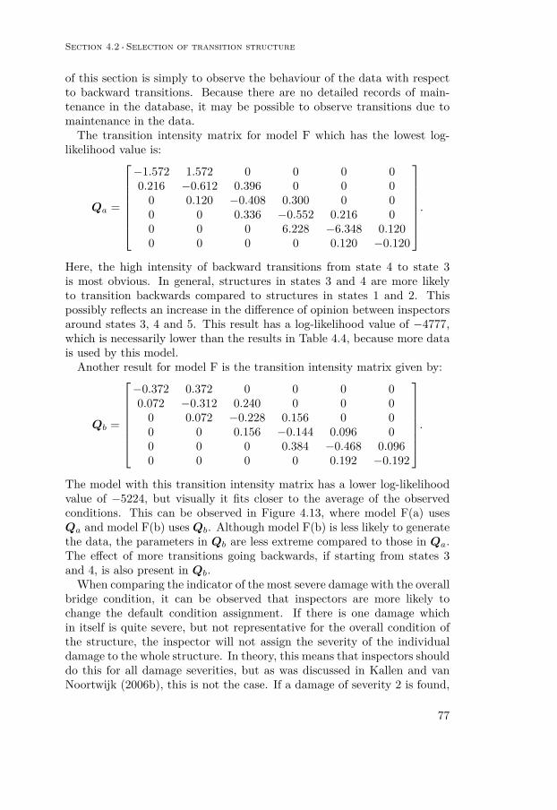
Section 4.2 · Selection of transition structure
77
of this section is simply to observe the behaviour of the data with respectto backward transitions. Because there are no detailed records of main-tenance in the database, it may be possible to observe transitions due tomaintenance in the data.
The transition intensity matrix for model F which has the lowest log-likelihood value is:
Qa =
−1.572 1.572 0 0 0 00.216 −0.612 0.396 0 0 0
0 0.120 −0.408 0.300 0 00 0 0.336 −0.552 0.216 00 0 0 6.228 −6.348 0.1200 0 0 0 0.120 −0.120
.
Here, the high intensity of backward transitions from state 4 to state 3is most obvious. In general, structures in states 3 and 4 are more likelyto transition backwards compared to structures in states 1 and 2. Thispossibly reflects an increase in the difference of opinion between inspectorsaround states 3, 4 and 5. This result has a log-likelihood value of −4777,which is necessarily lower than the results in Table 4.4, because more datais used by this model.
Another result for model F is the transition intensity matrix given by:
Qb =
−0.372 0.372 0 0 0 00.072 −0.312 0.240 0 0 0
0 0.072 −0.228 0.156 0 00 0 0.156 −0.144 0.096 00 0 0 0.384 −0.468 0.0960 0 0 0 0.192 −0.192
.
The model with this transition intensity matrix has a lower log-likelihoodvalue of −5224, but visually it fits closer to the average of the observedconditions. This can be observed in Figure 4.13, where model F(a) usesQa and model F(b) uses Qb. Although model F(b) is less likely to generatethe data, the parameters in Qb are less extreme compared to those in Qa.The effect of more transitions going backwards, if starting from states 3and 4, is also present in Qb.
When comparing the indicator of the most severe damage with the overallbridge condition, it can be observed that inspectors are more likely tochange the default condition assignment. If there is one damage whichin itself is quite severe, but not representative for the overall condition ofthe structure, the inspector will not assign the severity of the individualdamage to the whole structure. In theory, this means that inspectors shoulddo this for all damage severities, but as was discussed in Kallen and vanNoortwijk (2006b), this is not the case. If a damage of severity 2 is found,

Chapter 4 ·Application and results
78
bridge age [yr]
condit
ion s
tate
[−
]
0 10 20 30 40 50 60 70
54
32
10
Model F(a)Model F(b)Average state
Figure 4.13: Expected condition state formodel F, compared to the average state in thedata, using two sets of estimated parametervalues.
but the damage is not representative for the structure, the inspectors areless inclined to change the default condition assignment compared to if thedamage had a severity 3 or higher. This phenomenon is likely to be at leastone source of the backward transitions observed in model F.
Next, a model with perfect maintenance is considered. In this case,objects are allowed to transition back to the initial state. The estimatedtransition intensity matrix for this model, referred to as model ‘G’, is
Q =
−13.139 13.139 0 0 0 0
3.155 −4.041 0.886 0 0 00.069 0 −0.283 0.214 0 00.146 0 0 −0.266 0.120 01.326 0 0 0 −1.481 0.1550.426 0 0 0 0 −0.426
.
The expectation of the condition state as a function of the age of a structureis shown in Figure 4.14. The extremely high intensities out of state 0 andfrom state 1 back to state 0 are not very realistic. Nonetheless, this modelhas a log-likelihood of −4799, which is close to the likelihood of model Fwith transition intensity matrix Qa.
It is not unusual for the Dutch bridge condition data to result in fasttransitions out of the initial states. This is because the overall bridge condi-tion is very much like a series system in which the condition of the structure

Section 4.3 · Inclusion of inspection variability
79
bridge age [yr]
condit
ion s
tate
[−
]
0 10 20 30 40 50 60 70
54
32
10
Model GAverage state
Figure 4.14: Expected condition state formodel G, compared to the averag state in thedata.
is the same as the condition of the weakest link or element. As soon as asingle damage is found, the condition of the structure will transition out ofthe initial ‘perfect’ state. This is of course due to the automatic assignmentof the most severe damage indicator to the condition of the structure; seeSection 1.3.
4.3 INCLUSION OF INSPECTION VARIABILITY
The probabilities of observing a state Yk = j given that the true state isi at the k-th observation for each possible pair of states i and j, can becollected in an error or misclassification matrix:
E =
e00 e01 e02 e03 e04 e05e10 e11 e12 e13 e14 e15e20 e21 e22 e23 e24 e25e30 e31 e32 e33 e34 e35e40 e41 e42 e43 e44 e45e50 e51 e52 e53 e54 e55
, (4.2)
where eij = Pr{Yk = j |Xk = i}, therefore 0 ≤ eij ≤ 1 for all i and j, and∑j eij = 1. Note that eii is actually the probability of correctly identifying
state i as the current condition. Only eij for i 6= j represents a true misclas-sification. It is assumed here that the probabilities of misclassification donot change over time. Also, the error matrix is the same for all inspections,
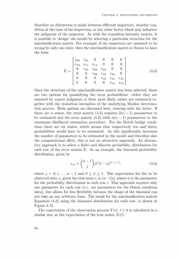
Chapter 4 ·Application and results
80
therefore no distinction is made between different inspectors, weather con-dition at the time of the inspection, or any other factor which may influencethe judgment of the inspector. As with the transition intensity matrix, itis possible to ‘design’ the model by selecting a particular structure for themisclassification matrix. For example, if the inspectors are assumed to bewrong by only one state, then the misclassification matrix is chosen to havethe form
E =
e00 e01 0 0 0 0e10 e11 e12 0 0 00 e21 e22 e23 0 00 0 e32 e33 e34 00 0 0 e43 e44 e450 0 0 0 e54 e55
. (4.3)
Once the structure of the misclassification matrix has been selected, thereare two options for quantifying the error probabilities: either they areassessed by expert judgment or their most likely values are estimated to-gether with the transition intensities of the underlying Markov deteriora-tion process. Both options are discussed here, starting with the latter. Ifthere are n states, the error matrix (4.3) requires 2(n − 1) parameters tobe estimated and the error matrix (4.2) adds n(n − 1) parameters to themaximum likelihood estimation procedure. For the Dutch bridge condi-tions there are six states, which means that respectively ten and thirtyprobabilities would have to be estimated. As this significantly increasesthe number of parameters to be estimated in the model and therefore alsothe computational effort, this is not an attractive approach. An alterna-tive approach is to select a finite and discrete probability distribution foreach row of the error matrix E. As an example, the binomial probabilitydistribution, given by
eij =(n− 1j
)φj(1− φ)n−j−1, (4.4)
where j = 0, 1, . . . , n − 1 and 0 ≤ φ ≤ 1. The expectation for the to beobserved state j, given the true state i, is (n−1)φ, where φ is the parameterfor the probability distribution in each row i. This approach requires onlyone parameter for each row (i.e., six parameters for the Dutch conditiondata), but allows for less flexibility because the shape of the binomial cannot take on any arbitrary form. The result for the misclassification matrixEquation (4.2) using the binomial distribution for each row, is shown inFigure 4.15.
The expectation of the observation process Y (t), t ≥ 0 is calculated in asimilar way as the expectation of the true states X(t):

Section 4.3 · Inclusion of inspection variability
81
bridge age [yr]
condit
ion s
tate
[−
]
0 10 20 30 40 50 60 70
54
32
10
Binomial est. meanAverage state
Figure 4.15: Expected condition state as afunction of age for the hidden Markov modelfitted to the overall bridge condition data.
EY (t) =∑j
j∑i
Pr{Y (t) = j |X(t) = i}Pr{X(t) = i}.
The result in Figure 4.15 looks similar to those in Figure 4.13. Due to thevariability in the inspections, the expected condition state may start in astate other than state 0. The estimated error matrix is
E =
0.19 0.37 0.30 0.12 0.02 0.000.13 0.32 0.33 0.17 0.04 0.010.04 0.19 0.33 0.29 0.13 0.020.03 0.15 0.31 0.32 0.16 0.030.15 0.35 0.32 0.14 0.03 0.010.04 0.19 0.33 0.29 0.13 0.02
The second option for quantifying the probabilities of misclassification,is to use expert judgment. In Sztul (2006) an informal expert judgmentapproach was applied. For the full error matrix Equation (4.2), two prob-ability distributions were chosen with a fixed mean: the binomial and themaximum entropy distributions. The basic assumption was that the expertis expected to correctly identify the true state, therefore the mean of eachrow distribution was set to the true state of that row. For the binomialdistribution, this results in an error matrix

Chapter 4 ·Application and results
82
E =
1.00 0.00 0.00 0.00 0.00 0.000.33 0.41 0.20 0.05 0.01 0.000.08 0.26 0.34 0.23 0.08 0.010.01 0.08 0.23 0.34 0.26 0.080.00 0.01 0.05 0.20 0.41 0.330.00 0.00 0.00 0.00 0.00 1.00
and for the maximum entropy distribution this results in
E =
1.00 0.00 0.00 0.00 0.00 0.000.48 0.25 0.13 0.07 0.04 0.030.25 0.21 0.17 0.15 0.12 0.100.10 0.12 0.15 0.17 0.21 0.250.03 0.04 0.07 0.13 0.25 0.480.00 0.00 0.00 0.00 0.00 1.00
.
The maximum entropy distribution is a discrete probability distributionwhich adds the least information (or which has maximum entropy) with agiven mean; see Jaynes (1957). It is less ‘informative’ than the binomialdistribution with given mean. The purpose of using the maximum entropydistribution is to add as little extra information as possible in order toobtain a result which is not too ‘colored’ by the choice of the error distrib-ution. Note that for both approaches, the first and last state are perfectlyobservable by the inspector. Another noticable effect of this approach isthat the inspectors would tend to underestimate the condition in the initialtrue states (i.e., states 1 and 2), whereas they would tend to overestimatethe condition in later states (i.e., states 3 and 4). From practical experi-ence in the Netherlands, this should be exactly the opposite in practice.See Sztul (2006) for the results of these two approaches.
4.4 ANALYSIS OF COVARIATE INFLUENCE
In Section 3.2.3, a short introduction to covariate analysis was given. Thepurpose of covariate analysis is to determine if a certain grouping of struc-tures, according to various characteristics, would result in significantly dif-ferent transition intensities. If this is the case, then the decision makermay choose to treat these groups separately in the maintenance model. Inthis section, a covariate analysis will be performed on the overall conditiondata from bridges in the Netherlands.
First, model A is considered with three covariates: whether a bridge islocated in or over the motorway, whether it is designated as a bridge orviaduct, and whether the structure is located in a province with a high orlow population intensity. In the Netherlands, a ‘bridge’ is generally definedas a structure over water and a ‘viaduct’ as a structure which connects

Section 4.4 ·Analysis of covariate influence
83
any two points in order to cross over an obstruction like, for example, amotorway. The log-linear model is then given by
λ = exp{β0 + β1X1 + β2X2 + β3X3},
where
X1 ={
0, if located in the motorway, and1, if located over the motorway.
X2 ={
0, if designated as a concrete viaduct, and1, if designated as a concrete bridge.
X3 ={
0, if located in a more densily populated province, and1, if located in a lesser populated province.
The null-hypothesis for each covariate is that it does not significantly in-fluence the model outcome; that is H0 : βi = 0. This hypothesis should berejected if the coefficient βi is significantly different from zero. The resultsfor model A are collected in Table 4.6. The last column in the table showsif the null-hypothesis is rejected or not. It is only rejected for β3 (even atthe 1% significance level), therefore this covariate (or independent variable)is significant. The other two covariates may influence the result as well,but from a statistical point of view this can not be shown with certainty.The null-hypothesis may also be rejected for coefficient β1 if consideringonly a 10% significance level, but this level is rarely used.
i β̂i SEβ̂i p-value reject
0 −4.2470 0.0291 n/a n/a1 0.0584 0.0388 0.07 no2 −0.0144 0.0475 0.38 no3 0.1529 0.0366 0.00 yes
Table 4.6: Estimated coefficients and theirstandard error and corresponding p-value forthe covariates in model A.
The base transition intensity is determined by the intercept β0. The basetransition intensity per month is exp{−4.2470} = 0.0143 or approximately0.17 per year. If the structure is located in a more densily populated area(i.e., X3 = 1) and does not possess the two other properties (i.e., X1 =X2 = 0), then this base intensity is multiplied with a factor exp{0.1529} =1.1652 per month and the annual transition intensity would be 0.20.
As mentioned in Chapter 3, the maximum likelihood estimator is as-ymptotically normal and in Section 3.2.3 it was mentioned that Wald’stest essentially rejects the hypothesis that β̂i = 0 if zero is not within the(1−α)% bounds. In Figure 4.16 it can be clearly observed how this resultsin the hypothesis β̂3 = 0 being rejected, whereas the others are not.

Chapter 4 ·Application and results
84
estimated coefficient value [−]
den
sity
[−
]
−0.4 −0.2 0.0 0.2 0.4
02
46
810
12
β̂1
β̂2
β̂3
Figure 4.16: Asymptotic density of thecoefficients for the explanatory variables inmodel A.
SUMMARY
The primary research goal was to see if Markov processes could be usedto model deterioration of structures in the Netherlands using the conditiondata which is available and to determine how this could best be done.This chapter describes the results of the maximum likelihood estimationprocedure introduced in the previous chapter.
The properties of the various data sets and how these were obtainedfrom the database, is the topic of Section 4.1. Three data sets have beenanalysed: overall bridge condition, condition of superstructures and ofkerbs. These data sets were extracted from the relational database usedin the Netherlands for the registration of inspection results. The databasewas not designed with a statistical analysis in mind, therefore the extrac-tion of the data and conversion into a suitable format for analysis requiresspecial care and a great deal of time.
For the models which allow only for deterioration (i.e., transitions toworse states), the quality of the fit onto the data increases as the number ofparameters increases. Age-dependent or inhomogeneous processes thereforetend to fit better due to the fact that they are more flexible to adapt to thedata and not necessarily because the data is age-dependent by nature. Froma practical point of view, model C, which has state-dependent transitionintensities (i.e., they may be different for each state), is the most appealingmodel, even if others have a higher likelihood of generating the given data.Optionally, model D may also be used. It allows for an overall change in

Section 4.4 ·Analysis of covariate influence
85
the transition intensities as a function of the structure’s age and requiresonly slightly more calculations to be made. However, the results indicatethat this change over time is not very strong, i.e. the intensities are closeto constant throughout a structure’s life.
If the possibility of backward transitions is included in the deteriorationprocess, to account for inspection variability or maintenance activities, thegeneral trend is that structures are more likely to move towards a worsestate in the initial states 0, 1 and 2, but the reverse is observed for states3, 4 and 5.
The inclusion of inspection variability, by use of hidden Markov mod-els, has been deemed not to be useful for application in the Netherlands.The probabilities of misclassification must be estimated from the data ordetermined by expert judgment. Either way, by definition of visual inspec-tions, the actual process can never be observed and therefore this processis completely determined by the subjective choice for the misclassificationprobabilities. For the Dutch bridge condition data, both the subjectiveestimation approach, and the data-based estimation, did not lead to sat-isfactory results. From a decision maker’s point of view, the subjectiveestimation approach is most likely to be preferred, as the data-based esti-mation may not result in a realistic misclassification structure. Also, thedata-based estimation introduces many more parameters to be estimated,which may pose a problem if the amount of data is insufficient.
Finally, a covariate analysis was performed to determine the significanceof the influence of independent variables. These independent variablesdescribe if a structure possesses a certain characteristic or not. In thisanalysis, three independent variables were considered: whether a bridge islocated within the motorway or over it, whether the structure is designatedto be a bridge or a viaduct and if the structure is located in a province witha relatively high population density. Only the latter has a statisticallysignificant influence, therefore separate maintenance policies may be usedfor structures in different locations throughout the country.


87
5Optimal maintenance decisions
Once the deterioration model, using a finite-state Markov process, has beenchosen and fitted to the available data, it can be used to make a decisionabout how often a structure should be inspected and which type of main-tenance should be performed at what time. This chapter therefore dealswith the decision model as discussed in Chapter 1 and shown in Figure 1.1.
For finite-state Markov processes, there are two decision models whichmay be used: a Markov decision process or a condition-based maintenancemodel. Markov decision processes are most commonly applied as they arepopular in general (Dekker, 1996). A short introduction to the theory ofMarkov decision processes is given in Section 5.1. The condition-basedmaintenance model is presented in Section 5.2 which is largely based onKallen and van Noortwijk (2006a). A comparison between both modelsis given, together with a discussion on the application of the condition-based maintenance model in the Netherlands, in the summary at the endof this chapter. The model presented here only considers the economicsof inspections and maintenance. In practice, thisis just one, albeit a veryimportant one, of many aspects to consider when deciding on a maintenancepolicy.
5.1 MARKOV DECISION PROCESSES
In order to be able to make decisions about an optimal policy for mainte-nance actions, a finite set of actions A and costs C(i, a) have to be intro-duced, which are incurred when the process is in state i and action a ∈ Ais taken. The costs are assumed to be bounded and a policy is defined tobe any rule for choosing actions. When the process is currently in state iand an action a is taken, the process moves into state j with probability
pij(a) = Pr{X(n+ 1) = j |X(n) = i, an = a}.
This transition probability again does not depend on the state history. If astationary policy is selected, then this process is called a Markov DecisionProcess (MDP). A stationary policy arises when the decision for an actiononly depends on the current state of the process and not on the time atwhich the action is performed.

Chapter 5 ·Optimal maintenance decisions
88
Now that the state of the structure over time with or without perform-ing maintenance actions can be modeled, the optimization of inspectionand maintenance policies using this process can be performed. For exam-ple, when the system is in state i, the expected discounted costs over anunbounded horizon are given by the recurrent relation
Vα(i) = C(i, a) + αN∑j=1pij(a)Vα(j), (5.1)
where α is the discount factor for one year and Vα is the value functionusing α. This discount factor is defined as α = (1 + r/100)−1 with r theyearly discount percentage. Starting from state i, Vα(i) gives us the cost ofperforming an action a given by C(i, a) and adds the expected discountedcosts of moving into another state one year later with probability pij(a).The discounted costs over an unbounded horizon associated with a start instate j are given by Vα(j), therefore Equation (5.1) is a recursive equation.The choice for the action a is determined by the maintenance policy andalso includes no repair.
A cost optimal decision can now be found by minimizing Equation (5.1)with respect to the action a. A classic approach is to use a policy improve-ment algorithm, which consists of successively adjusting the policy untilno further improvement can be made. Under some minor assumptions,this optimization problem can also be formulated as a linear programmingproblem, which can then be solved using the simplex algorithm. See Ross(1970, Chapter 6) for the theory of Markov decision processes.
A Markov decision process and the linear programming formulation wasused in the Arizona pavement management system, see Golabi et al. (1982)and Golabi (1983), and in Pontis, see Golabi and Shepard (1997), amongstothers. More references are given in the review by Frangopol et al. (2004).
5.2 CONDITION-BASED INSPECTION AND MAINTENANCE MODEL
The Markov decision processes discussed in the previous section, are es-sentially condition-based decision models as the decisions depend on thecurrent state of the process. The model which will be discussed in this sec-tion is commonly referred to simply as the ‘condition-based inspection andmaintenance model’ for stochastic processes, hence the title of this section.
5.2.1 MODEL
As discussed in Chapter 1, each maintenance model can be roughly sepa-rated into a deterioration model and a decision model. For the application

Section 5.2 ·Condition-based inspection and maintenance model
89
10 10
10 10
0 1 · · · r − 1 functional states
r · · · s − 1 marginal states
s · · · m failed states
Figure 5.1: Graphical representation of themarginal checking model.
of the decision model, the structure of the Markov deterioration process isdefined first.
Deterioration model
For the deterioration model, a sequential Markov process is used. Anew object starts in state 0 and successively degrades through subsequentstates as is shown in Figure 5.1. States r and s are the threshold statesfor preventive and corrective maintenance respectively. An object whichhas not yet reached state r is functional and if it has reached state r, butnot yet state s, it is called marginal. States s and beyond are failed states.The term ‘marginal’ was used in the same context by Flehinger (1962) andindicates that the object is still functional, but is ready for a preventiverepair or replacement.
Decision model
The decision model is based on renewal theory. It is therefore assumedthat preventive and corrective repairs bring the object to an as-good-as-new state. The time between the service start of an object and its renewalrepresents a single life cycle. The renewal reward process R(t) is defined as
R(t) =N(t)∑n=1Yn,
where Yn is the reward earned at the n-th renewal. In the context of main-tenance, the rewards are the costs of inspection and maintenance actions.The goal of the decision model is to minimize the long-term expected av-erage costs per unit of time given by limt→∞ ER(t)/t. According to therenewal reward theorem,

Chapter 5 ·Optimal maintenance decisions
90
limt→∞
ER(t)t
= ECEI, (5.2)
where C are the uncertain costs per cycle and I is the uncertain durationof a cycle; see for example Ross (1970, p.52). The expected average costsper unit of time over an unbounded horizon are therefore given by the ratioof the expected total costs incurred during the life cycle over the expectedlength of a life cycle. It is also possible to consider discounted costs in orderto account for inflation over longer periods of time. However, for ease ofpresentation, discounting is not considered here.
Let τ > 0 denote the fixed duration between inspections, such that kτ(k = 1, 2, . . .) is the time of the k-th inspection. This is the primary decisionvariable. Other decision variables like the threshold state r for preventivemaintenance may be included. Also, the time to the first inspection, assuggested by Jia and Christer (2002), is a useful decision variable. In thiscase, the inspections are performed at times τ1 + (k − 1)τ for k = 1, 2, . . .and the optimal combination of τ1 and τ , resulting in the lowest expectedaverage costs per unit of time, are determined.
At each inspection, the object can be in a functional, marginal or failedstate. If the object is found to be in a functional state, no maintenance isrequired and only the cost of the inspection is incurred. If it is found tobe in a marginal state, the costs of preventive maintenance are added tothe cost of the inspection. For an object in a failed state, there are twoscenarios: either the failure is immediately noticed at the time of occur-rence, without the necessity of an inspection, or failure is only detected atthe next planned inspection. In the first case, only the costs of correctivemaintenance are incurred and in the second case, the costs of the inspectionand unavailability have to be included as well.
The costs per cycle are the sum of the costs of all inspections duringthe cycle and either a single preventive or a single corrective replacement.For the first scenario, in which failure is immediately noticed, the expectedcycle costs are
EC =∞∑k=1
[(kcI + cR) Pr{PR in ((k − 1)τ, kτ ]}+ · · ·
+ ((k − 1)cI + cF ) Pr{CR in ((k − 1)τ, kτ ]}], (5.3)
where PR is preventive repair, CR is corrective repair, and cI , cP and cFare the costs of an inspection, preventive repair and a corrective repairrespectively. The expected cycle length is

Section 5.2 ·Condition-based inspection and maintenance model
91
EI =∞∑k=1
[kτ Pr{PR in ((k − 1)τ, kτ ]}+ · · ·
+kτ∑
n=(k−1)τ+1
nPr{CR in (n− 1, n]}]. (5.4)
The summation over n from (k − 1)τ + 1 to kτ reflects the immediateidentification of a failure.
For the second scenario, in which failure is not noticed until the nextinspection, Equations (5.3) and (5.4) become
EC =∞∑k=1
[(kcI + cR) Pr{PR in ((k − 1)τ, kτ ]}+ · · ·
+ (kcI + cF ) Pr{CR in ((k − 1)τ, kτ ]}+ · · ·
+kτ∑
n=(k−1)τ+1
cU (kτ − n) Pr{failure in (n− 1, n]}], (5.5)
and
EI =∞∑k=1
[kτ Pr{PR in ((k − 1)τ, kτ ]}+ · · ·
+ kτ Pr{CR in ((k − 1)τ, kτ ]}], (5.6)
where cU are the costs of unavailability per unit time. This cost is addedin Equation (5.5) as a penalty for leaving a structure in a failed state. Thecosts increase proportionally to the time that the object is left in the failedstate. Without this cost, the cheapest solution would be to not inspect atall, because the average costs per unit of time will decrease as the cyclelength increases.
5.2.2 PROBABILITIES OF PREVENTIVE AND CORRECTIVE MAINTENANCE
Special case
In this section, the most simple type of Markov process, namely the state-independent and time-homogeneous Markov process is considered, whichcorresponds to model A as defined in Section 4.2.1. In this case, thewaiting times are modeled by identical exponential distributions, that is,T ∼ Exp(λ) with FT (t) = 1− exp{−λt}. Let Sn =
∑ni=1 Ti be the time at
which the n-th transition takes place, then the following equivalence holds:

Chapter 5 ·Optimal maintenance decisions
92
X(t) ≤ n⇔ Sn ≥ t
In words: if the state of the object is less than or equal to n at time t,the time required to perform n transitions is greater than or equal to t.Note that for a component with sequential condition states as depictedin Figure 5.1, Sn is also the first passage time of state n. Using thisrelationship, the probability of preventive repair becomes
Pr{PR in ((k − 1)τ, kτ ]} = Pr{(k − 1)τ < Sr ≤ kτ, Ss > kτ}.
This is the probability that the threshold state r for preventive mainte-nance is first reached between the previous inspection at time (k− 1)τ andthe current inspection at time kτ , and the threshold state s for correc-tive maintenance has not been reached before the current inspection. Theanalytical solution of this probability is
Pr{(k − 1)τ < Sr ≤ kτ, Ss > kτ} =s−r−1∑j=0
(λkτ)j+r
(j + r)!e−λkτ
[1− I1− 1
k(r, j + 1)
], (5.7)
where
Ix(a, b) =∫ xφ=0
Γ(a+ b)Γ(a)Γ(b)
φa−1(1− φ)b−1dφ
is the incomplete beta function for 0 ≤ x ≤ 1, a > 0 and b > 0, see forexample Abramowitz and Stegun (1965). The result in Equation (5.7) isobtained by splitting the probability and using the independence of theincrements Sr and Ss − Sr:
Pr{(k − 1)τ < Sr ≤ kτ, kτ − Sr < Ss − Sr}= Pr{Sr ≤ kτ, kτ − Sr < Ss − Sr} − · · ·− Pr{Sr ≤ (k − 1)τ, kτ − Sr < Ss − Sr}.
Denoting the difference of these two probabilities by A− B, each of thesecan be calculated as follows:

Section 5.2 ·Condition-based inspection and maintenance model
93
A =∫ kτφ=0
∫ ∞θ=kτ−φ
fSr (φ)fSs−Sr (θ)dθdφ
=∫ kτφ=0fSr (φ)
[∫ ∞θ=kτ−φ
fSs−Sr (θ)dθ]
dφ
=∫ kτφ=0
λrφr−1e−λφ
(r − 1)!
s−r−1∑j=0
λj(kτ − φ)j
j!e−λ(kτ−φ)
dφ
=s−r−1∑j=0
[λ(j+r)
(j + r)!e−λkτ (kτ)j+r−1 × · · ·
×∫ kτφ=0
(j + r)!(r − 1)!j!
(1− φkτ
)j (φ
kτ
)r−1dφ
].
With the substitution ϕ = φkτ , the beta function integrates out:
A =s−r−1∑j=0
[λ(j+r)
(j + r)!e−λkτ (kτ)j+r−1kτ
∫ 1
ϕ=0
(j + r)!(r − 1)!j!
(1− ϕ)jϕr−1dϕ
]
=s−r−1∑j=0
(λkτ)j+r
(j + r)!e−λkτ .
The same calculations can be used to derive the second part:
B =s−r−1∑j=0
(λkτ)j+r
(j + r)!e−λkτI1− 1
k(r, j + 1).
The difference A−B results in Equation (5.7).For a corrective repair, the state at the previous inspection was again
less than r, but is greater than or equal to the failure state s at time kτ .This probability is given by
Pr{CR in ((k − 1)τ, kτ ]} = Pr{Sr > (k − 1)τ, (k − 1)τ < Ss ≤ kτ}
and in this case becomes
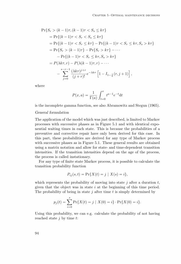
Chapter 5 ·Optimal maintenance decisions
94
Pr{Sr > (k − 1)τ, (k − 1)τ < Ss ≤ kτ}= Pr{(k − 1)τ < Sr < Ss ≤ kτ}= Pr{(k − 1)τ < Sr ≤ kτ} − Pr{(k − 1)τ < Sr ≤ kτ, Ss > kτ}= Pr{Sr > (k − 1)τ} − Pr{Sr > kτ} − · · ·− Pr{(k − 1)τ < Sr ≤ kτ, Ss > kτ}
= P (λkτ, r)− P (λ(k − 1)τ, r)− · · ·
−s−r−1∑j=0
(λkτ)j+r
(j + r)!e−λkτ
[1− I1− 1
k(r, j + 1)
],
where
P (x, a) = 1Γ(a)
∫ xt=0ta−1e−tdt
is the incomplete gamma function, see also Abramowitz and Stegun (1965).
General formulation
The application of the model which was just described, is limited to Markovprocesses with successive phases as in Figure 5.1 and with identical expo-nential waiting times in each state. This is because the probabilities of apreventive and corrective repair have only been derived for this case. Inthis part, these probabilities are derived for any type of Markov processwith successive phases as in Figure 5.1. These general results are obtainedusing a matrix notation and allow for state- and time-dependent transitionintensities. If the transition intensities depend on the age of the process,the process is called instationary.
For any type of finite state Markov process, it is possible to calculate thetransition probability function
Pij(s, t) = Pr{X(t) = j | X(s) = i},
which represents the probability of moving into state j after a duration t,given that the object was in state i at the beginning of this time period.The probability of being in state j after time t is simply determined by
pj(t) =s∑i=0
Pr{X(t) = j | X(0) = i} · Pr{X(0) = i}.
Using this probability, we can e.g. calculate the probability of not havingreached state j by time t:

Section 5.2 ·Condition-based inspection and maintenance model
95
Pr{X(t) < j} =j−1∑i=0
Pr{X(t) = i} =j−1∑i=0pi(t).
To calculate the probability of a preventive or corrective repair, the currentstate of the deterioration process is used instead of the first passage time asin the special case described before. The probability of a preventive repairis the probability that the object was in a functional state at the previousinspection (i.e., X((k − 1)τ) < r) and in a marginal state at the currentinspection (i.e., r ≤ X(kτ) < s):
Pr{PR in ((k − 1)τ, kτ ]} = Pr{r ≤ X(kτ) < s,X((k − 1)τ) < r}. (5.8)
Similarly, the probability of corrective repair is the probability of the objectbeing in a failed state at the current inspection when it was still in afunctional state at the previous inspection:
Pr{CR in ((k − 1)τ, kτ ]} = Pr{X(kτ) ≥ s,X((k − 1)τ) < r}. (5.9)
Equation (5.8) can be split up in two parts:
Pr{r ≤ X(kτ) < s,X((k − 1)τ) < r}= Pr{X(kτ) < s,X((k − 1)τ) < r} − · · ·− Pr{X(kτ) < r,X((k − 1)τ) < r}.
Denoting this difference as A − B, each probability can be calculated asfollows:
A = Pr{X(kτ) < s,X((k − 1)τ) < r}= Pr{X(kτ) < s | X((k − 1)τ) < r} Pr{X((k − 1)τ) < r}
=s−1∑j=0
Pr{X(kτ) = j | X((k − 1)τ) < r} Pr{X((k − 1)τ) < r}
=s−1∑j=0
r−1∑i=0
Pr{X(kτ) = j | X((k − 1)τ) = i} Pr{X((k − 1)τ) = i}
=s−1∑j=0
r−1∑i=0Pij((k − 1)τ, kτ)pi((k − 1)τ)
and similarly

Chapter 5 ·Optimal maintenance decisions
96
B = Pr{X(kτ) < r,X((k − 1)τ) < r}= Pr{X(kτ) < r | X((k − 1)τ) < r} · Pr{X((k − 1)τ) < r}
=r−1∑j=0
Pr{X(kτ) = j | X((k − 1)τ) < r} · Pr{X((k − 1)τ) < r}
=r−1∑j=0
r−1∑i=0Pij((k − 1)τ, kτ)pi((k − 1)τ).
Using these results, Equation (5.8) simplifies to
A−B =s−1∑j=r
r−1∑i=0Pij((k − 1)τ, kτ)pi((k − 1)τ). (5.10)
Using the same approach and the knowledge that s is the final state, Equa-tion (5.9) can be simplified as follows:
Pr{X(kτ) ≥ s,X((k − 1)τ) < r}= Pr{X(kτ) = s | X((k − 1)τ) < r} · Pr{X((k − 1)τ) < r}
=r−1∑i=0
Pr{X(kτ) = s | X((k − 1)τ) = i} · Pr{X((k − 1)τ) = i}
=r−1∑i=0Pis((k − 1)τ, kτ)pi((k − 1)τ). (5.11)
Note that results (5.10) and (5.11) are valid for all types of Markov process-es. For example, if we are using stationary Markov processes with time-independent transition rates, the transition functions Pij((k−1)τ, τ) reduceto Pij(τ). These algorithmic formulations can therefore also be used toobtain the same results as are obtained using the analytical formulationsin previous part.
The probability of a failure in the interval (n− 1, n] for n starting at thefirst year after the previous inspection, being (k − 1)τ + 1, to the time ofthe current inspection, being kτ , is given by the following:

Section 5.2 ·Condition-based inspection and maintenance model
97
Pr{X((k − 1)τ) < r,X(n− 1) < s,X(n) = s}= Pr{X(n− 1) < s,X(n) = s |X((k − 1)τ) < r} × · · ·× Pr{X((k − 1)τ) < r}
=r−1∑i=0
Pr{X(n− 1) < s,X(n) = s |X((k − 1)τ) = i} × · · ·
× Pr{X((k − 1)τ) = i}
=r−1∑i=0
(Pis(n)− Pis(n− 1)
)pi((k − 1)τ).
The probability of failure during each year in the interval ((k − 1)τ, kτ ]is therefore conditional on the probability that no preventive repair wasperformed at the start of this interval.
5.2.3 APPLICATION TO DUTCH BRIDGE CONDITION DATA
Two hypothetical scenarios are considered with fictitious costs presented inTable Table 5.1.
Scenario A Scenario B
Failure detection immediate by inspectionInspection (cI) ¤1000 ¤1000Prev. repair (cP ) ¤10000 ¤10000Corr. repair (cF ) ¤40000 ¤10000Unavailability (cU ) N/A ¤2000
Table 5.1: Costs for two hypothetical ex-amples.
Scenario A considers the case in which a failure is immediately detectedand repaired without the need for an inspection. The costs for a correctiverepair are four times the costs of a preventive repair, therefore it will beeconomically interesting to repair before failure occurs. Scenario B consid-ers the other case, in which failure is not detected until the next inspectionand a cost is incurred for each unit of time that the superstructure is in afailed state. For both scenarios, the threshold for preventive repair is stater = 3 and the failed state is state s = 5. The unit time considered in bothscenarios is one year.
Scenario B suits the case of superstructures very well, because state 5 isconsidered to be a condition failure and not an actual physical failure andtherefore an inspection is required to assess the state of the superstructure.

Chapter 5 ·Optimal maintenance decisions
98
inspection interval [yr]
cost
[E
UR
/yr]
0 10 20 30 40 50 60 70 80
040
080
012
0016
00
Scenario AScenario BMinima
Figure 5.2: Expected average costs peryear for superstructure maintenance as a func-tion of the inspection interval τ and usingmodel A.
For the bridge superstructures, the results for both scenarios are shown inFigure 5.2.
Since in scenario A corrective repair is expensive compared to preventiverepair, the inspection interval with lowest expected average costs per yearis shorter than the same optimal value for scenario B: 6 years comparedto 13 years. With a mean time to preventive repair of r/λ ≈ 16.7 years.This implies that about 3 inspections are performed for scenario A anda preventive repair is done after about 18 years. For scenario B, onlyabout 2 inspections are performed and a repair is performed after about26 years. As τ → ∞, the costs in scenario A converge to the costs ofa corrective repair, ¤40000, divided by the expected lifetime of 28 years,which is approximately ¤1430. The costs in scenario B do not converge,but increase every year due to the cost of unavailability.
The cost model presented in this section is easier to implement thanthe classic policy improvement algorithm, which is used for Markov de-cision processes. Instead of presenting the decision maker with a singleoptimal value, this approach results in a clear graphical presentation as isdemonstrated by Figure 5.2. Also, the models can be adjusted for varioussituations. For example, Equations (5.3) to (5.6) can be adjusted to includediscounting, see e.g. van Noortwijk et al. (1997), or to include the time ofthe first inspection as an extra decision variable. The latter extension hasbeen demonstrated before by Jia and Christer (2002) and is useful whenthe thresholds for preventive and corrective maintenance are very close to

Section 5.2 ·Condition-based inspection and maintenance model
99
each other. When the difference in costs for preventive or corrective re-placement is large, this would result in a very short inspection interval,which would be unnecessary when the structure has just been taken intoservice. The model will determine the optimal combination of the time offirst inspection and the subsequent periodic inspection interval.
Another extension is to include the threshold state for preventive main-tenance as a decision variable. The optimal inspection intervals and thecorresponding expected average costs per year for r ranging from state 1to 4, are shown in Table 5.2.
Threshold Example A Example Br τ EC/EI τ EC/EI
[yr] [¤/yr] [yr] [¤/yr]
1 14 985 21 6722 10 887 19 6413 6 855 13 6024 4 1026 9 592
Table 5.2: Optimal inspection intervals fordifferent preventive maintenance thresholdlevels.
For example A, r = 3 is optimal and for example B r = 4 is optimal.In example B, the cost of a corrective repair is the same as the cost of apreventive repair, therefore the model minimizes the expected number ofpreventive renewals. This is achieved by placing the threshold for preven-tive repair as close as possible to the threshold for corrective repair, whichis state 5 in this case. In general, the optimal length of the inspection in-terval τ becomes smaller as the threshold is moved closer to the thresholdof a corrective renewal. As the margin for preventive maintenance becomessmaller, more frequent inspections are required to increase the probabilityof performing a preventive repair instead of a corrective repair. If r = 4is chosen in example A, the risk of missing the opportunity for preventiverepair becomes much greater and this results in a higher expectation forthe average costs per year.
In the previous chapter, it was observed that a state-dependent model,namely model C, fits better to the bridge condition data compared to thestate-independent model A, which is applied above. For superstructures,the estimated parameters for model C are listed in Table 4.5. Using thegeneral formulation of the condition-based inspection model, the expectedaverage costs per year are calculated using model C for superstructures.The result for both scenarios as defined in Table 5.1, is shown in Figure 5.3.
The optimal inspection interval for scenario A is 15 years with ¤654 peryear and 23 years for scenario B with ¤498 per year. Because the mean

Chapter 5 ·Optimal maintenance decisions
100
inspection interval [yr]
cost
[E
UR
/yr]
0 10 20 30 40 50 60 70 80
040
080
012
0016
00
Scenario AScenario BMinima
Figure 5.3: Expected average costs peryear for superstructure maintenance as a func-tion of the inspection interval τ and usingmodel C.
times to reach the threshold states are longer in comparison with thosegiven by model A, the times between inspections are also longer. However,the minima of both results are much less defined. For scenario A, theexpected costs using an inspection interval of 10 or 20 years are only slightlymore compared to the expected average costs per year for the optimalinterval length of 15 years. This is a result of the much larger uncertaintyin the amount of time it takes to reach the treshold states. In this case,the decision maker must make a decision with care. Using other criteria,like past experience or just common sense, he may decide for a shorter orlonger period of time between inspections than the optimum given by themodel. To aid in his decision, he may also calculate the variance of theresults in Figures 5.2 and 5.3, which would give an indication about theconfidence bounds around the mean. Explicit formulas for this purpose aregiven by van Noortwijk (2003) for the condition-based inspection modelwhich includes discounting. Experience with the variance of the averagecosts per time unit, show that a choice for a shorter inspection intervalgenerally has a smaller variance and is therefore less risky. So the decisionmaker might choose an inspection interval of 10 years for scenario A andabout 20 years for scenario B.

Section 5.3 · Survival probability
101
5.3 SURVIVAL PROBABILITY
If no information on the cost of different maintenance actions is available,then a more simplistic approach to inspection planning could be used. Adecision maker often needs to make a decision about whether or not astructure needs an earlier inspection than planned. For example, he mayhave a structure which is quite old, but has been reported to be in a goodstate. Not considering any life-cycle costs, he may want to assess the riskof a ‘failure’ before the next periodic inspection. For this purpose, thesurvival probability curves may be computed and reviewed by the decisionmaker. The selection of an inspection interval based on an acceptable risklevel, is commonly used in risk-based inspection methodologies; see Kallenand van Noortwijk (2005a) for an introduction to risk-based inspection inthe process and refining industry.
If T is the random variable representing the uncertain time to failure,the survival probability of a structure, given that it has survived up to ages, is defined as Pr{T > t |T > s}. In other words, it is the probability ofsurviving up to age t conditional on having survived up to age s, where0 ≤ s ≤ t. A simple derivation shows that
Pr{T > t |T > s} = Pr{T > t}Pr{T > s}
= S(t)S(s),
where S(t) = 1 − F (t) = Pr{T > t} is the common notation for thesurvival probability function. For the finite-state Markov processes usedhere, the probability of failure is defined as the probability of reachingthe final absorbing state, namely state 5. The ‘survival’ probability atage t is the probability of being in any state other than state 5 at age t:S(t) ≡ Pr{X(t) 6= s}. For the sequential Markov process in Figure 5.1,this probability is
S(t) = Pr{X(t) < 5} =4∑i=0
Pr{X(t) = i} = p′0 exp{Rt}1,
where the matrix notation uses the fact that this probability distributionis a phase-type distribution as introduced in Section 2.1.3.
As an example, the survival probability curve of superstructures in state0 at ages 0, 25, 50, 75, and 100, are calculated and shown in Figure 5.4.The survival curve for superstructures at age 0 is simply the random timerequired for a superstructure to reach state 5 from state 0, which has a meanof about 43 years as listed in Table 4.5. It is obvious that as superstructuresreach higher ages, their remaining life shortens. However, the remaininglife does not converge to zero, which is clearly observed in Table 5.3. Thisresult is not entirely surprising, because it takes a minimum amount of

Chapter 5 ·Optimal maintenance decisions
102
remaining time [yr]
pro
bab
ilit
y [−
]
0 20 40 60 80 100 120
0.0
0.2
0.4
0.6
0.8
1.0
0 years25 years50 years75 years100 years
Figure 5.4: Survival probability curves forsuperstructures in the initial state 0 at variousages.
age mean remaining time[yr] [yr]
0 42.725 24.750 19.575 17.8100 17.1
Table 5.3: Mean time for superstructuresto reach state 5 from state 0 at various ages.
time for a structure (or any object), which is in a perfect state at an oldage, to reach the final state.
SUMMARY
Although both a Markov decision process and the model presented in Sec-tion 5.2 are condition-based decision models, they are different in many as-pects. The most fundamental difference between them, is that the Markovdecision processes are used to optimize the maintenance policy given afixed inspection interval, whereas the condition-based model presented inSection 5.2 is used to optimize the length of the inspection interval givena fixed policy. The maintenance policy of the latter model is to performa preventive repair or replacement if the structure is in a marginal state

Section 5.3 · Survival probability
103
and to perform a corrective repair or replacement if it is in a failed state.The length of time between inspections for the Markov decision processesdescribed in Section 5.1 is implicitly included in the transition probabilityfunction Pij(a). If the policy of a Markov decision process is chosen toemulate the marginal checking policy of the model in Section 5.2, the timebetween inspections may be optimized by calculating the value functionVα(i) using different time periods for Pij(a).
A successful application of the condition-based maintenance model pre-sented in this chapter depends on a number of aspects. First of all, theremust be some relationship between the state in which the structure orcomponent is and how much it costs to bring this object back to an as-good-as-new state. This is currently not possible for bridge condition datain the Netherlands, as there is no direct relationship between the condi-tion state and the size and type of damages. This is due to the fact thatdiscrete condition states are used for quantifying visual assessments of theoverall condition of an object and not for sizing individual damages. Thequote on page 23 formulates this rather well. This feature has significantconsequences as it implies that practically all data in this form can not beused for an exact estimation of maintenance costs.
Another aspect which affects the applicability of a maintenance model,is the quality of the data. The aspect of data quality was discussed at thebeginning of Chapter 4 and it is the registration of maintenance activitieswhich is especially important in the context of maintenance optimization. Ifthe data is of sufficient quality and the costs of maintenance are quantified,the condition-based model presented in Section 5.2 is easy to implementand easy to use. The implementation is straightforward compared to thatof a Markov decision process and the results can be presented to decisionmakers in a simple plot like those in Figures 5.2 and 5.3.
Finally, it was shown in Section 5.3 how the survival curve of an objectmay be used to assess the risk of a ‘failure’ before the next inspection. Thesurvival probability is calculated based on the current age and state of theobject. This approach does not consider the costs of maintenance over thelife-cycle of the object, but merely serves as an additional decision tool forthe decision maker.


105
6Conclusions and recommendations
In short, the research goal was to implement and test a suitable model formodeling the rate of deterioration for bridges in the Netherlands. There areover 3000 concrete bridges in the Netherlands, which are managed by theCivil Engineering Division of the Ministry of Transport, Public Works andWater Management. It is their duty to ensure the safety of the users andthe availability of the road network by inspecting and maintaining thesebridges. Due to an aging bridge stock and increasing demands on account-ability, a structured approach to the planning and scheduling of mainte-nance activities is required. The primary uncertainty in the optimizationof maintenance activities is the uncertainty in the rate of deterioration ofstructures. The approach presented in this research is aimed at the appli-cation of a model which uses the available condition data to quantify thisuncertainty and therefore to aid in the decision making process.
SPECIFICATION
The approach advocated in this thesis, is of statistical nature and the firststep in any statistical analysis is the specification of a model as a gener-ator of the given data. As seen in Section 1.2.2, it is also possible to usea physics-based approach where the deterioration is explicitly modeled bya ‘physical’ model. The reason for choosing a statistical approach is theavailability of a large data set with bridge condition states obtained byinspections over a period of almost twenty years. Also, physical measure-ments are infeasible at such a large scale.
To represent the uncertain development of the state of a structure, orone of its components over time, a finite-state Markov process (also knownas a ‘Markov chain’) is used. This choice is quite common in civil engi-neering applications and also in medical studies, where the condition of astructure or patient is categorized according to a discrete and finite condi-tion scale. For infrastructure in the Netherlands, a scale with seven statesgiven in Table 1.1 is used. The use of a discrete condition scale is due tothe visual nature of the inspections. The large number of structures in thenetwork makes it too costly to perform actual damage size measurementson a regular basis. In the case of medical studies, there is often no deviceto measure the actual extent of a disease, therefore an expert assessment

Chapter 6 ·Conclusions and recommendations
106
is made using the information which is available. The reliability of a struc-ture is traditionally used as a measure of the quality of a structure. Thisreliability depends on the ability of the structure to carry the loads that areplaced upon it, which makes it a typical stress-strength model. There is nodevice to measure the reliability of a structure or component, therefore itmust be calculated using the information available to the decision maker.
A Markov process is a stochastic process for which the Markov propertyholds. This property can be roughly defined as the property where thefuture state of the process is independent of the past given the presentstate. The assumption is therefore that all information from the past iscontained in the current state of the process. In the past, there has beensome debate within the bridge management community about the validityof this assumption. In statistical analysis, and especially in the contextof maximum likelihood estimation, there is no ‘true’ model. The qualityof a model is primarily determined by the likelihood of such a model gen-erating the given data. Because all assumptions are made by choice, thedecision maker may also use other subjective criteria to select a model forhis purposes.
In Section 2.4, the testing of the Markov assumption is shortly addressed.For the available condition data in the Netherlands, obtained by periodicinspections, it is not practically feasible to test the validity of the Markovproperty in the data. The discrete nature of the data and the fact that sucha large collection of data is available, weighs more heavily in the choice for aMarkov process than the question of whether or not the Markov assumptionis valid.
ESTIMATION
The Markov model used in this research is a parametric model, which meansthat there are a finite number of parameters. The Markov process itselfis shaped by its transition structure, which is defined by the transitionprobability matrix or transition intensity matrix. Because a continuous-time Markov process is applied to the Dutch bridge condition data, a largepart of the modeling aspect is the estimation of the transition intensities(or ‘rates’).
Chapter 3 reviews various aspects of the maximum likelihood estimationapproach, which is used to fit the continuous-time Markov process to thepanel data obtained by periodic visual inspections. These aspects includethe consideration of uncertainty and variability in the inspection resultsand the testing of the influence of independent variables on the outcome.The maximum likelihood approach presented in Chapter 3 is different fromprevious approaches which are found in the literature and most of whichare reviewed in Section 2.3. Contrary to many of the reviewed estimation

107
procedures, the maximum likelihood method is particularly well suited forpanel data, because it does not depend on the exact times of transitions,nor on the exact duration of stay in any particular state. It only uses thelikelihood of observing a structure in a particular state at a particular age,which is exactly the information available to the decision maker.
APPLICATION
Since 1985, a database to record inspections and maintenance activitieson infrastructure in the Netherlands has been in use. In 2004, this data-base contained over 6000 observations of concrete bridge state conditions,which can be used to estimate the model parameters. The database wasnot specifically designed for use in a statistical analysis, therefore the datahad to be prepared first. The process of preparing the data for appli-cation in a Markov model, consisted of filtering out faulty or incompletedata entries and converting the data set to a suitable format for the es-timation procedure. Details on the data and the extraction process aregiven in Section 4.1. Experience with the Dutch database shows that theextraction process requires a great deal of attention and care in order toensure the quality of the data set. Although this particular database isdesigned and used only by the Ministry of Transport, Public Works andWater Management in the Netherlands, it is very likely that databases inother countries or with a different application (like e.g., in sewer systemand pavement management) will also require a significant effort in order tocreate a usable data set.
A Markov process is shaped by the transition probability or transitionintensity matrix, therefore the layout of the transition structure is anotherdecision for the modeler to make. The transition structure may be chosensuch that only deterioration is possible (resulting in a ‘progressive’ process)or such that transitions towards better condition states are also allowed for.A progressive or sequential model should be used to model deterioration,since bridge conditions can not physically improve without intervention inthe form of maintenance. Because of their rare application, self-healingmaterials are not considered here.
Age-dependent transition intensities
Existing Markov models in bridge management systems do not incorporatetime-dependent transition probabilities or intensities. The approach pre-sented here allows age-dependence to be included in a fairly straightforwardmanner. Unlike with semi-Markov processes, the dependence is not on thelength of stay in a condition state, but rather on the age of the structureor the component. This allows the transition intensities to increase as thedeteriorating object ages. It does not increase the probability of a pending

Chapter 6 ·Conclusions and recommendations
108
transition if the duration of stay in a condition state increases. As men-tioned in Section 2.5, the latter feature results in a very complicated modelwhich is not analytically tractable.
The addition of age-dependence results in a significantly better fit tothe bridge condition data; see Section 4.2.1. However, this should notbe considered as proof that bridge deterioration is age-dependent or non-homogeneous. It is only proof that the extra parameter helps to make themodel fit closer to the observations. As for testing the Markov property, thecondition data does not have sufficient detail for testing time-homogeneity.
Inspection variability
The inclusion of inspection variability is a topic which has received consid-erable interest, especially in combination with Markov decision processes.These approaches are referred to as ‘partially observable’ or ‘latent’ Markovdecision processes. In the area of speech recognition, a Markov process withobservational errors is called a hidden Markov model. The same terminol-ogy is used here, as the application of inspection variability is not combinedwith Markov decision processes. The primary goal in this research is totest if hidden Markov models are a useful extension to the regular Markovprocesses. The most challenging aspect of this model is to estimate theprobability of misclassification. This is the probability of observing one ofthe condition states given a true underlying state. It may be estimatedusing the data itself or it may be determined by expert judgment.
In the end, hidden Markov models are not deemed to be suitable forapplication in bridge deterioration modeling. This is primarily due to thefact that, by the definition of visual inspections, the true state can never bemeasured and therefore not be used to check the quality of the estimatedparameters. The course of the true state is completely determined by thechoice for the misclassification probabilities and this choice is subjective.
Influence of independent variables
Although no two bridges will be exactly alike, most concrete bridges in theNetherlands can be considered to be similar in terms of design, constructionmaterial and usage. Nonetheless, it is possible to group bridges according tovarious characteristics. For example, bridges constructed using box girdersmay be considered separately from bridges with a beam supported roadsurface. It is also possible to group bridges according to their geographicallocation. Since the statistical analysis depends on the availability of asufficient amount of data, it is important that the resulting groups do notcontain a too small number of structures. In order to decide whether ornot to consider certain groups of bridges, a statistical test of significancecan be performed to determine if the groups behave significantly different.

109
If not, then it is not necessary for the decision maker to treat these groupsdifferently in the maintenance model.
The maximum likelihood method is well suited to perform a so-called‘covariate analysis’, where the influence of the independent variables (i.e.,the variables which describe if a structure possesses a certain characteristicor not) on the outcome can be measured. From the Dutch database, threepossible groups where identified in Section 4.4: 1) whether or not a bridgeis located in the motorway, 2) whether the structure is identified as a‘bridge’ or a ‘viaduct’, and 3) if the structure is located in a provincewith a relatively high population number. Only the last group behavessignificantly different from structures located in provinces with a lowerpopulation number. When determining a maintenance policy, the decisionmaker may therefore include the province in which the structure is locatedas an additional variable.
Maintenance and inspection decisions
Chapter 5 is completely devoted to decision models which may be appliedwhen using a finite-state Markov process as a deterioration model. Theclassical approach to optimizing maintenance decisions is to use a Markovdecision process. An easy alternative condition-based maintenance modelis presented in Section 5.2. This model balances the costs of inspectionsand preventive maintenance against the costs of corrective maintenance todetermine the optimal time between inspections. It also allows the decisionmaker to determine the optimal threshold for preventive maintenance. Twoscenarios have been evaluated in a case study using the deterioration modelobtained in Chapter 4. In the first scenario, the bridge is found to be in anunacceptable state without the necessity of performing an inspection. Thesecond scenario considers a more realistic situation where an inspectionis required to observe if the structure has reached an unacceptable stateor not. A penalty is applied for every year that a structure is left in anunacceptable state.
Because these decision models minimize the costs of inspections andmaintenance over the lifetime of a structure, it is necessary to have repre-sentative cost data. Since the condition states used in bridge inspections donot represent a measure of the extent of damage, it is difficult to determinethe cost of repairing structures in different states.
IMPLEMENTATION
In this project, special attention has been put into the aspects of the im-plementation of the maximum likelihood estimation and the maintenancemodel. Due to the large amount of state observations, it is not necessaryto estimate the model parameters anew after every inspection. The model

Chapter 6 ·Conclusions and recommendations
110
is sufficiently robust such that significant changes in the parameter valuesare not to be expected. Nonetheless, a model for which the computationstake too much time is not very appealing to the demanding user of to-day. Therefore, Chapter 7 deals with various techniques to calculate thetransition probability function. This function gives the probability of tran-sitioning between any two states during a specified period of time and ifthe transition intensities are age-dependent, this function will also dependon what age this period starts.
Out of all the reviewed approaches to calculating the transition prob-ability function, uniformization is the most appealing. This particularapproach enables an algorithmic calculation in which both the transitionprobability function and its derivatives may be calculated simultaneously.Also, other than scalar operations, the uniformization technique only con-sists of matrix multiplications and additions (or substractions), thereforeavoiding relatively complicated calculations like the inversion of matrices.This feature makes it quite easy to implement the model in any program-ming language.
IN RETROSPECT
Several questions were defined in the introduction on page 12, which willbe shortly addressed here:
a. it has indeed proven possible to extract condition data from the data-base in order to subject it to a statistical analysis.
b. most of the statistical models and estimation methods proposed forapplication to bridge maintenance, are reviewed in Chapter 2, but nonepossess all the properties that are desired for the Dutch situation.
c. a continuous-time Markov process is a suitable stochastic process formodeling the deterioration of structures. It is not as simplifying asa discrete-time Markov process and it not as intractable as a semi-Markov process with non-exponential waiting times. A likelihood func-tion, which consists of a product of transition probabilities, has beendefined. The method of maximum likelihood estimation is most suitedfor this non-linear model.
d. a bootstrapping procedure indicates that the model is robust to changesin the data. The estimates for the model parameters do not deviatevery much when using different data sets obtained by bootstrappingthe original data set.
e. the uniformization method is particularly efficient and well suited forcalculating the transition probability function. Also, its relationship tothe Poisson process enables the calculation of the transition probabilityfunction up to a specified accuracy.

111
f. the chosen model estimates that it takes about 45 years for a concretebridge to reach state 5, which is a state at which major renovation isgenerally required. Due to the large variability in the many factorswhich influence the state of a structure, this estimate is very uncertain.With 90% probability, the time required to reach the fifth state is rouglybetween 14 and 96 years.
g. selecting different groups of bridges according to various characteristicsin most cases did not result in significantly different estimates for themodel parameters. Only a selection of structures according to the pop-ulation density of the province in which they are located, resulted insignificantly different transition intensities.
h. although it may seem interesting to explicitly model inspection vari-ability in the model, the use of a hidden Markov model turned out tobe practically infeasible. The primary problem is that the true state ofthe structure is never known, therefore it is quite difficult to determinethe amount of misclassification by an inspector. Only expert judgmentmay be able to offer a quantification of the inspection errors.
i. for finite-state Markov processes, a suitable condition-based inspectionand maintenance model has been defined. It determines the inspectioninterval with lowest expected average costs per time unit. A require-ment for the application of such a model is that the costs of preventiveand corrective repairs are available to the decision maker.
RECOMMENDATIONS
For the particular case of bridge management in the Netherlands, thereare several recommendations for the application of the model proposed inthis thesis. The first is to better record any maintenance activities in thedatabase, such that backward transitions can more easily be related toeither maintenance or inspection variability. This will allow to filter outmaintenance data such that the deterioration model can be estimated using‘clean’ condition data. Also, if maintenance activities can be filtered out,the application of a hidden Markov model for inspection variability may bepossible. With the present data this did not result in satisfactory results.The application of such a model may also be made easier if inspectors doc-ument their reasoning behind the choice of a condition state. For example,if the inspector assigns a better condition to the structure compared to theprevious inspection, he could indicate if this is because maintenance wasperformed after the previous inspection or not. In any case, this type ofadditional information should be given as a finite number of options bythe system to the inspectors. It is not possible to automate the filtering ofcondition data if inspectors are allowed to supply their information in theform of unrestricted textual comments.

Chapter 6 ·Conclusions and recommendations
112
The database in the Netherlands contains a sufficient number of stateobservations for the application of the maximum likelihood estimation. Thebootstrap procedure discussed in the section entitled “Distribution of theestimated parameters” on page 71, can be used to test if the estimatordisplays normality (i.e., if it is Gaussian). This test is particularly valuablefor those states which are less frequently observed. However, the bootstrapis a computationally expensive procedure and it is important to ensure thatthe accurracy of the calculations is sufficiently high such that the outcomeis not distorted. This research did not consider the situation where verylittle or no condition data is available. For those applications where this isthe case, a Bayesian approach could be developed.
This research has shown that a finite-state Markov process is very wellsuited for use in a Dutch bridge management system. In order to completethe maintenance model with a decision model, it is necessary to develop adependable cost model. This means that the costs of various maintenanceactions must be quantified as a function of the existing condition state, thetype of component or building material, and the age of the structure. Thisis a challenging problem because the condition rating scheme is specificallydesigned not to represent the actual size of damages. Past experience, com-bined with expert judgment, can be used to estimate maintenance costs.
The inspection intervals which are obtained using the condition-basedmaintenance model presented in Section 5.2, are often quite long. This isbecause the policy is assumed to start at the service start of the structureand structures deteriorate relatively slow. In most cases, structures arenot new at the time of the analysis and have already undergone one ormore inspections. Shorter and more reasonable inspection intervals maybe obtained by adding the first inspection as a separate decision variableor by starting from the current state and age of the structure. The latter ismathematically possible due to the memoryless property of the continuous-time Markov process.
Finally, the problem at hand is a typical problem of decision makingunder uncertainty. Inspections are a tool to gain more information andtherefore to reduce the uncertainty in the rate of deterioration of struc-tures and their elements. However, it is not possible to acquire completeinformation and there is no true model to predict the lifetimes of struc-tures. The best recommendation is therefore to use common sense whenmaking any decision!

113
7Appendix: transition probability function
Define the transition probability function as
pij(s, t) = Pr{X(t) = j |X(s) = i}. (7.1)
This function gives the probability of moving from state i at time s ≥ 0 tostate j a period t− s ≥ 0 later. Let P (s, t) = ‖pij(s, t)‖ be the transitionprobability function matrix. P (s, t) = I for all s ≥ 0 if t = s and P (s, t)is stochastic, that is:
∑j pij(s, t) = 1 for all i. If the process is time-
homogeneous, then P (s, t) = P (0, t − s) with the equivalent shorthandnotation defined as
pij(0, t− s) ≡ pij(t− s) = Pr{X(t− s) = j |X(0) = i}. (7.2)
This chapter deals with how to efficiently calculate the transition prob-ability function and its sensitivity towards the model parameters. Theparameters in the context of Markov processes are the transition intensi-ties which, as is the case for inhomogeneous Markov processes, may be afunction of the process age.
7.1 HOMOGENEOUS MARKOV PROCESSES
7.1.1 KOLMOGOROV EQUATIONS
The transition probability function is the solution to the forward andbackward Kolmogorov equations. For a continuous-time Markov processwith constant transition intensities, these are given by P ′(t) = P (t)Qand P ′(t) = QP (t) respectively. The well known solution to these dif-ferential equations is the matrix exponential as defined in Equation (2.6):P (t) = exp{Qt}. There are a number of ways to show that this is the so-lution to the Kolmogorov equations. One approach is to use the transitionprobability function in Equation (2.4) and use a Laplace transformationto derive this result, see e.g., Howard (1971). The set of linear differentialequations defined by the Kolmogorov equations can also be solved by themethod of successive approximations. This is demonstrated next.
Take the backward Kolmogorov equations, then these define a boundaryvalue problem of the form

Chapter 7 ·Appendix: transition probability function
114
X ′ = QX, X(0) = I,
where I is the identity matrix. Assume that a solution X = P (t) exists,then the integral equation
P (t) = I +∫ tu=0QP (u) du (7.3)
is equivalent to the boundary value problem in the sense that any solu-tion of one is also a solution of the other. This can easily be verified bysetting t = 0 to obtain the initial condition P (0) = I and by taking thederivative towards t to obtain the set of differential differential equationsP ′(t) = QP (t). The derivation can be done because the solution P (t) isassumed to be a continuous function andQ is constant over the range of in-tegration. The initial approximation is the boundary condition P (0)(t) = I.Substitution into Equation (7.3) yields the second approximation
P (1)(t) = I +∫ tu=0QP (0)(u) du = I +Qt+Q2 t
2
2.
Through proof by induction, it is straightforward to show that
P (n)(t) = I +Qt+Q2 t2
2+ · · ·+Qn t
n
n!for n → ∞. Then, by the definition of the matrix exponential in Equa-tion (2.6), P (n)(t)→ exp{Qt}.
7.1.2 MATRIX EXPONENTIAL
The definition of the matrix exponential in Equation (2.6) is restated here:
exp{Qt} = I +Qt+Q2 t2
2!+Q3 t
3
3!+ · · · (7.4)
Although the calculation of the matrix exponential may look trivial, it iscertainly not. The formulation as an infinite series is an analytical result,but in practice it is impossible to calculate an infinite number of terms.A quasi analytical solution is to calculate the infinite series up to a large,but finite number of terms. According to Moler and van Loan (1978), thestandard Taylor series approximation, achieved by truncating the infiniteseries in Equation (7.4) after a convergence criterion has been reached, isslow and prone to errors if a low floating point accuracy is used. The errorsare due to rounding during the matrix multiplication and these in turn area result of the presence of both positive and negative elements in the matrixQ, see e.g., Ross (2000, p.350).

Section 7.1 ·Homogeneous Markov processes
115
There are many ways to calculate the matrix exponential and Châteletet al. (1996) grouped these in three categories:
1. numeric: integration methods for ordinary differential equations likee.g., the Euler and Runga-Kutta schemes,
2. analytical: e.g., using the Laplace transformation and the method basedon matrix diagonalization,
3. quasi or partially analytical: e.g., exponential limit method and uni-formization.
Matrix diagonalization
Assume that A is a square matrix of size n × n and has n linearly inde-pendent eigenvectors, then the matrix A is diagonalizable, i.e., it can bewritten in the form A = PDP−1, where D is a diagonal matrix. Matrixdiagonalization is equivalent to finding the eigenvalues (and the eigenvec-tors) of A, because the eigenvalues form the diagonal in D. If A can bediagonalized, it holds that
exp{A} = P exp{D}P−1,
where exp{D} is easily obtained by exponentiating the elements in thediagonal of D. The method of matrix diagonalization for calculating theexponential of a square matrix is an analytical method. A sufficient con-dition for the matrix A to be diagonalizable, is that no two eigenvaluesare the same (i.e., all n eigenvalues have multiplicity 1). By definitionthis excludes the possibility to model sequential continuous-time Markovprocesses with identical waiting times in each state. Other models may nothave this problem, but numerical procedures as part of a maximum likeli-hood estimation may incidentally result in (nearly) identical eigenvalues.
Uniformization
Uniformization, also known as randomization, is a fairly well known wayof computing the matrix exponential for Markov processes, see e.g., Tijms(2003) or Kohlas (1982). This approach is essentially an adapted Taylorseries approximation. The uniformization technique makes the series ap-proximation converge faster, avoids the rounding errors due to the negativeelements in Q, and also has a nice probabilistic interpretation.
Using the transition intensity matrix Q with elements defined in Equa-tion (2.7), a new discrete-time Markov process Xt is generated by settingthe one-step transition matrix to
pij ={
1− λi/λ, if i = j,(λi/λ)pij , if i 6= j,

Chapter 7 ·Appendix: transition probability function
116
where λ ≥ λi for all i. If we now define a new continuous-time Markovprocess like X(t) = XN(t), then we get a Markov process where the tran-sition times are generated by a Poisson process with rate λ > 0 and statetransitions are generated by pij . Whereas the process with intensity matrixQ (possibly) has a different rate for each state i, the new process has anintensity matrix Q with the same rate λ for each state:
qij ={−λ, if i = j,λpij , if i 6= j.
If we use matrix notation, we say that P = Q/λ+ I and we can calculatethe matrix exponential as
P (0, t) = eQt = eλt(P−I) = eλtP e−λtI =∞∑k=0e−λt
(λt)k
k!Pk. (7.5)
For the fastest convergence of the series approximation, λ should be chosenas small as possible, but no smaller than the largest λi, otherwise P willnot be a stochastic matrix (i.e., not all rows sum to one). The best choiceis therefore λ = maxi λi.
When approximating Equation (7.5) by calculating the series up to k =M , the truncation error is given by the remainder of the series:
r1(λ, t,M) =∞∑
k=M+1e−λt
(λt)k
k!Pk.
In order to determine how large M should be, it is necessary to assess thesize of the truncation error. For this purpose, it is possible to calculate anupper bound for the error and this requires a matrix norm. Heidelbergerand Goyal (1988) incorrectly use a matrix 1-norm, whereas the matrixinfinity norm (maximum absolute row sum) defined as
‖A‖∞ = maxi
∑j
|Aij |, (7.6)
is better suited, because ‖P k‖∞ = 1 for all k = 0, 1, 2, . . . . Using the trian-gular inequality with the matrix norm, the upper bound of the truncationerror is
‖r1(λ, t,M)‖∞ ≤∞∑
k=M+1‖P k‖∞e−λt
(λt)k
k!= 1− Pλt(M),
where Pφ(n) is the cumulative Poisson distribution with parameter φ ≥ 0.So using Equation (7.6), the error r1(λ, t,M) is conveniently bounded by
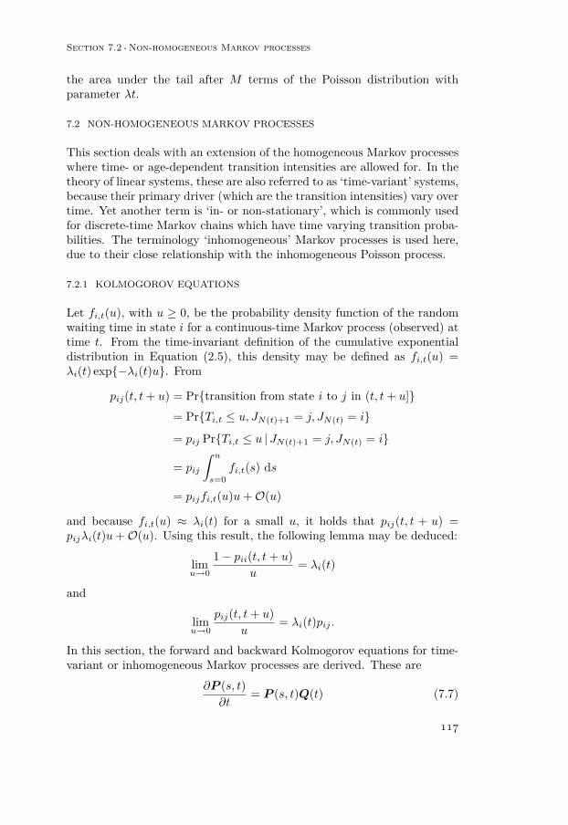
Section 7.2 ·Non-homogeneous Markov processes
117
the area under the tail after M terms of the Poisson distribution withparameter λt.
7.2 NON-HOMOGENEOUS MARKOV PROCESSES
This section deals with an extension of the homogeneous Markov processeswhere time- or age-dependent transition intensities are allowed for. In thetheory of linear systems, these are also referred to as ‘time-variant’ systems,because their primary driver (which are the transition intensities) vary overtime. Yet another term is ‘in- or non-stationary’, which is commonly usedfor discrete-time Markov chains which have time varying transition proba-bilities. The terminology ‘inhomogeneous’ Markov processes is used here,due to their close relationship with the inhomogeneous Poisson process.
7.2.1 KOLMOGOROV EQUATIONS
Let fi,t(u), with u ≥ 0, be the probability density function of the randomwaiting time in state i for a continuous-time Markov process (observed) attime t. From the time-invariant definition of the cumulative exponentialdistribution in Equation (2.5), this density may be defined as fi,t(u) =λi(t) exp{−λi(t)u}. From
pij(t, t+ u) = Pr{transition from state i to j in (t, t+ u]}= Pr{Ti,t ≤ u, JN(t)+1 = j, JN(t) = i}
= pij Pr{Ti,t ≤ u |JN(t)+1 = j, JN(t) = i}
= pij∫ us=0fi,t(s) ds
= pijfi,t(u)u+O(u)
and because fi,t(u) ≈ λi(t) for a small u, it holds that pij(t, t + u) =pijλi(t)u+O(u). Using this result, the following lemma may be deduced:
limu→0
1− pii(t, t+ u)u
= λi(t)
and
limu→0
pij(t, t+ u)u
= λi(t)pij .
In this section, the forward and backward Kolmogorov equations for time-variant or inhomogeneous Markov processes are derived. These are
∂P (s, t)∂t
= P (s, t)Q(t) (7.7)

Chapter 7 ·Appendix: transition probability function
118
and
∂P (s, t)∂s
= −Q(s)P (s, t) (7.8)
respectively. Either one of these two equations can be used to describe thedynamics in time of the Markov process. Given a transition rate matrixQ(t), the Kolmogorov equations give the solution to the transition proba-bility function P (s, t). In other words: the characteristics of the Markovprocess are determined by the choice for Q(t) and P (s, t) is determined bysolving one of the Kolmogorov equations Equation (7.7) and Equation (7.8).The Chapman-Kolmogorov equations are given by
pij(s, t) =∑k
pik(s, s+ u)pkj(s+ u, t), (7.9)
where s ≤ s+ u ≤ t. From Equation (7.9) we obtain
pij(s+ u, t)− pij(s, t) =∑forallk 6=i
−pik(s, s+ u)pkj(s+ u, t) +[1− pii(s, s+ u)
]pij(s+ u, t).
Hence,
limu→0
pij(s+ u, t)− pij(s, t)u
= limu→0
{∑k 6=i−[pik(s, s+ u)
u
]pkj(s+ u, t) + · · ·
+[
1− pii(s, s+ u)u
]pij(s+ u, t)
}.
The limit can be taken inside the summation (see for example Ross (1970))to reveal the backward Kolmogorov equations:∂
∂spij(s, t) =
∑k 6=i−λi(s)pikpkj(s+ u, t) + λi(s)pij(s+ u, t). (7.10)
Define
qij(t) ={−λi(t), if i = j,λi(t)pij , if i 6= j. (7.11)
Using Q(t) = ‖qij(t)‖, Equation (7.10) can be written in the matrix nota-tion given by Equation (7.8).
For the forward Kolmogorov equation, a similar approach can be usedto derive Equation (7.7). Using the Chapman-Kolmogorov equation againwith s ≤ t− u ≤ t, the following result is obtained:

Section 7.2 ·Non-homogeneous Markov processes
119
pij(s, t)− pij(s, t− u) =∑k 6=jpik(s, t− u)pkj(t− u, t)−
[1− pjj(t− u, t)
]pij(s, t− u).
Dividing both sides by u and taking the limit u→ 0, a scalar representationof the forward Kolmogorov equation is obtained:
∂
∂tpij(s, t) =
∑k 6=jpik(s, t− u)λk(t)pkj − λj(t)pij(s, t). (7.12)
Using the definition Equation (7.11) and a matrix notation, Equation (7.12)results in Equation (7.7).
It is tempting to write
P (s, t) = exp{∫ tu=sQ(u) du
}(7.13)
with
exp{∫ tu=sQ(u) du
}=
I +∫ tu=sQ(u) du+ 1
2
∫ tu=sQ(u) du
∫ tv=sQ(v) dv + · · ·
as the solution for nonhomogeneous Markov processes, like Howard (1971)did on page 843. Unfortunately this is not a general solution, which canbe easily shown by taking the derivative (Kailath (1980, Chapter 9)):
∂
∂texp{∫ tu=sQ(u) du
}=
Q(t) + Q(t)2
∫ tu=sQ(u) du+
∫ tv=sQ(v) dvQ(t)
2+ · · ·
6= exp{∫ tu=sQ(u) du
}Q(t).
The solution in Equation (7.13) only holds if Q(t) and∫Q(u)du commute,
which is not the case for most practical applications. The true general solu-tion may be found in using a similar approach as with the homogeneous casein Section 7.1.1. Equivalent to Equation (7.3) for the time-homogeneousprocess, the solution of the forward Kolmogorov Equation (7.7) may bewritten in the form of an integral equation:
P (s, t) = I +∫ tu=sP (s, u)Q(u) du. (7.14)

Chapter 7 ·Appendix: transition probability function
120
The successive approximations are:
P (0)(s, t) = I,
P (1)(s, t) = I +∫ tt1=t0Q(t1) dt1,
P (2)(s, t) = I +∫ tt2=t0Q(t2) dt2 +
∫ tt2=t0
{∫ t2t1=t0Q(t1) dt1
}Q(t2) dt2
up to
P (n)(s, t) = I +∫ tt2=t0Q(t2) dt2 +
∫ tt2=t0
{∫ t2t1=t0Q(t1) dt1
}Q(t2) dt2,
. . .+∫ ttn=t0
∫ tntn−1=t0
· · ·∫ t2t1=t0Q(t1)Q(t2) · · ·Q(tn) dt1 dt2 · · · dtn.
where s = t0 < t1 < · · · < ti < · · · < tn ≤ t. If n → ∞, then P n(s, t) →P (s, t) and the resulting series approximation
P (s, t) = I + · · · (7.15)
+∞∑n=1
∫ ttn=t0
∫ tntn−1=t0
· · ·∫ t2t1=t0Q(t1)Q(t1) · · ·Q(tn) dt1 dt2 · · · dtn,
is known as the Peano-Baker series. Convergence of this successive approx-imation is proven by Dacunha (2005) for the standard problem x′(t) =A(t)x(t),x(t0) = x0 in the theory of linear systems. It should be no sur-prise that, for a stationary process with Q(t) = Q, the Peano-Baker seriessolution in Equation (7.15) reduces to
P (0, t) = I +Qt+Q2 t2
2!+Q3 t
3
3!+ · · · ,
which is, of course, the same as the result in Equation (2.6). This Taylorseries solution has no intuitive (i.e., probabilistic) interpretation, thereforethe Peano-Baker series solution in Equation (7.15) does not either. But,as in the stationary case, uniformization can be used to transform thissolution to one with a probabilistic interpretation.
7.2.2 PRODUCT INTEGRATION
The formulation of the transition probability function in Equation (7.14) asan integral equation is merely an equivalent formulation of the solution tothe forward Kolmogorov equations defined in Equation (7.7). The integralequation does not actually give the solution, it merely reformulates the

Section 7.2 ·Non-homogeneous Markov processes
121
problem itself. In this section, another formulation is introduced: theproduct integral, which is denoted by
P (s, t) = R(s,t]
(I +Q( dτ)), (7.16)
where I is the identity matrix and Q(t) the transition intensity matrix asa function of time t. The notation P was suggested by Gill and Johansen(1990) and is related to the product
∏like the integral
∫is related to the
sum∑
.The formal definition of the product integral is the following:
R(0,t]
(1− f( dt)) = limmaxi |ti−ti−1|→0
∏i
(1− (f(ti)− f(ti−1)))
where the limit is taken over a sequence of ever finer partitions of theinterval [0, t]. The function f must be a real valued, cadlag function ofbounded variation, defined on the finite interval [0, t] ⊂ R. The definitionmay be extended to cases with more than two states. Let F be a n ×n matrix valued function of bounded variation in which each componentis right continuous with left hand limits. The product integral over theinterval [0, t] is now simply defined as
R(0,t]
(I + F (dt)) = limmaxi |ti−ti−1|→0
∏i
(I + F (ti)− F (ti−1)).
As is proven in Gill and Johansen (1990), the transition probability ma-trix defined in Equation (7.16) using the product integral has the requiredproperties, i.e.
− P (s, t) is a stochastic matrix, since each row sums to one,− P (s, t) = P (s, u)P (u, t) for 0 ≤ s ≤ u ≤ t ≤ ∞,− P (s, s) = I with 0 ≤ s and− P (s, t)→ I as t ↓ s.
Most importantly, it is shown by Gill and Johansen (1990) that the productintegral defined in Equation (7.16) is the unique solution to the forward andbackward Kolmogorov equations. The transition probability matrices forboth the continuous-time Markov process (with constant transition rates)and the discrete-time Markov process (with transitions at fixed discretetime points) are special cases of P (s, t). This can be easily shown and isdone in the next section.
Special cases
Consider the continuous-time Markov process with transition intensity ma-trix Q. We want to derive that P (s, t) = P (0, t − s) ≡ P (t − s) =

Chapter 7 ·Appendix: transition probability function
122
exp{Q(t − s)}, similar to Equation (2.6). If we define an equidistant par-tition on the interval [s, t]: s = t0 < t1 < t2 < . . . < tN−1 < tN = t withti = s+ i(t− s)/N , then
P (s, t) = limN→∞
N∏i=1
(1 +Q(ti)−Q(ti−1))
= limN→∞
N∏i=1
[1 + Q(t− s)
N
]
= limN→∞
[1 + Q(t− s)
N
]N(7.17)
= exp{Q(t− s)},
which is the well known solution for continuous-time Markov processes. Ifwe assume that transitions can only occur at discrete points in time, we geta discrete-time Markov process. Assume that s, t = 0, 1, 2, . . . with s < tand let N = t − s such that the interval has partitions of size 1. Since Nis fixed, Equation (7.17) reduces to P (s, t) = [I +Q]t−s. As
qij = limdt↓1
Pr{X( dt) = j |X(0) = i} = Pr{X(1) = j |X(0) = i} = pij
for i 6= j and qii = −∑j 6=i pij , we get that P (s, t) = P t−s. This is
again the familiar solution for discrete-time Markov chains (with P beingthe one-step transition probability matrix) under the assumption that theprocess is stationary (or time-homogeneous).
7.2.3 EULER SCHEME
The transition probability function P (s, t) is the solution to the forwardand backward Kolmogorov equations, which are differential equations forwhich many numerical approximation techniques exist. The Euler schemeis the most simple technique which approximates the derivative with a finitedifference. For example, for the forward Kolmogorov Equation (7.7) thismeans that [
P (s, t)− P (s, t−∆t)]∆t−1 = P (s, t−∆t)Q(t),
which yields
P (s, t) = P (s, t−∆t)(Q(t)∆t+ I)
for t ≥ s + ∆t and with a sufficiently small step size ∆t. A standardprocedure for the application of the Euler scheme is to partition the time

Section 7.2 ·Non-homogeneous Markov processes
123
interval [s, t] in N parts, such that ∆t = (t − s)/N and tk = s + ∆t fork = 0, 1, . . . , N . The transition probability function may then be iterativelyapproximated starting with P (s, s) = I and continuing with P (s, tk) =P (s, tk−1)(Q(tk)∆t+ I), k = 1, 2, . . . , N .
The efficiency of this approach of course depends on ∆t. The step sizemust be chosen sufficiently small to ensure adequate accuracy, but a verysmall step size will require a large number of matrix multiplications. Notethe similarity of the Euler scheme with the approach used in the sectiontitled “Special cases” on page 121 for the product integral. Approximatingthe product integral formulation of the transition probability function inEquation (7.16) with a large, but finite, number of products is therefore thesame as approximating the Kolmogorov equations using the Euler scheme.
7.2.4 UNIFORMIZATION
Similar to van Moorsel and Wolter (1998), P (t) = Q(t)/λ+ I can be usedto derive the uniformization equation for inhomogeneous Markov processes.Starting from the Peano-Baker series in Equation (7.15) this results in:
P (s, t) = (7.18)∞∑n=0
(λt)n
n!e−λt∫ ttn=t0
∫ tntn−1=t0
· · ·∫ t2t1=t0P (t1) · · ·P (tn)
n!tn
dt1 · · · dtn,
where λ > 0 is now chosen such that
λ ≥ inft∈(s,t]
|Qij(t)|.
Equation (7.18) represents a inhomogeneous Markov process where thetransition times occur according to a Poisson process with rate λ > 0 andtransitions in the embedded Markov chain are performed according to P (t).The product P (t1)P (t2) · · ·P (tn) is the n-step probability of transitionsoccurring at times {t1, t2, . . . , tn}. The integration is done over all possiblesets {t1, t2, . . . , tn} and n!/tn is the density of the order statistic of an n-dimensional uniform distribution resulting from the Poisson process. Thepaper by van Moorsel and Wolter (1998) continues with an algorithm tocompute Equation (7.18), but it is clear that this is not a simple thing todo.
There is one way to reduce the complexity of Equation (7.18) and thatis to choose the transition intensity matrix such that it can be decomposedlike Q(t) = f(t)Q. In this way, we end up with a transition probabilitymatrix for the embedded Markov chain which does not depend on time,i.e., P = Q(t)/f(t) + I = Q + I. As was pointed out by Rindos et al.(1995), Equation (7.13) is now a correct solution and it is possible to write

Chapter 7 ·Appendix: transition probability function
124
P (0, t) = exp{QΛ(t)} = exp{(Q+ I)Λ(t)− IΛ(t)} =∞∑n=0PnΛ(t)n
n!e−Λ(t),
or, more general,
P (s, t) =∞∑n=0Pn [Λ(t)− Λ(s)]n
n!e−[Λ(t)−Λ(s)], (7.19)
where Λ(t) =∫ tu=0 f(u) du. Now we have a inhomogeneous Poisson process
generating the transition times and P defining the transitions of the em-bedded Markov chain. This approach can only be used if the transitionintensity matrix is of the form Q(t) = Qf(t), where Q is a time-invariant(or constant) matrix and f(t) ≥ 0 is a scalar function of t. An example ofa matrix which is of this form is
Q(t) =
−a1t
b a1tb 0 0 0 0
0 −a2tb a2t
b 0 0 00 0 −a3t
b a3tb 0 0
0 0 0 −a4tb a4t
b 00 0 0 0 −a5t
b a5tb
0 0 0 0 0 0
,
where f(t) = tb.
7.3 PARAMETER SENSITIVITY
In order to maximize the likelihood function, which includes the matrix ex-ponential as the transition probability function, it is necessary to assess thesensitivity of the model towards changes in the parameter values. For this,it is required to calculate the derivative of the matrix exponential towardseach of the parameters contained in the transition matrix Q. These deriva-tives can then be used to implement an iterative approximating scheme tofind the values of the parameters which maximize the likelihood function.If λ = {λ1, . . . , λn} is a vector of all parameters contained in Q(t), thepartial derivative towards one of these parameters is given by
∂
∂λiP (s, t) =
∫ tu=sP (s, u)∂Q
∂λiP (u, t) du. (7.20)
For a stationary Markov process with constant Q, this becomes
∂
∂λiexp{Qt} =
∫ tu=0e(t−u)Q ∂Q
∂λieuQ du, (7.21)
which according to Tsai and Chan (2003) is due to Wilcox (1967). It isinteresting to see the similarity with the case of a Markov chain. If we
Section 7.3 ·Parameter sensitivity
125
assume P is a one-step transition probability matrix, then the derivativeof the n-step probability towards the parameter λi is
∂P n
∂λi=n−1∑k=0P k(∂P
∂λi
)P n−1−k.
The fact that Equation (7.21) holds for the derivative and not the wellknown result for the scalar case, can easily be shown as follows:
∂
∂λiexp{Qt} =
∞∑k=0
∂Qk
∂λi· tt
k!=∞∑k=0
[n−1∑i=0Qi(∂Q
∂λi
)Qk−1−i
]tk
k!
6= exp{Qt} · ∂Q∂λi,
where the partial derivative of Q towards λi can not be taken outside thesummation due to the fact that matrix multiplication is not commutative(i.e., the order of multiplication of matrices can generally not be changed:AB 6= BA).
7.3.1 MATRIX DIAGONALIZATION
Here, the exact analytical derivative of P (s, t) towards the parameters inQ(t) will be derived under the assumption that Q(t) can be decomposedinto f(t)Q as in the previous section.
The approach is based on the principle that the intensity matrix maybe decomposed as Q = ADA−1, where D is a diagonal matrix with theeigenvalues of Q on the diagonal and the columns of A are the eigenvectorsof Q. Using diagonalization, the matrix exponential can be simplified asfollows:
P (s, t) = exp{Q
∫ tu=sf(u) du
}= A exp{D[Λ(t)− Λ(s)]}A−1.
For ease of notation, let E = exp{D[Λ(t) − Λ(s)]} with elements ei =exp{di[Λ(t) − Λ(s)]}, i = 1, . . . , n on the diagonal, where di is the i-thdiagonal element of matrix D. In Kalbfleisch and Lawless (1985), thederivation for ∂P /∂θi is included, but the following essential steps, takenfrom Jennrich and Bright (1976), are not mentioned in the derivation.Using the product rule for differentiation and a shorthand notation dP (s, t)for the partial derivative of the transition probability function towards oneof the parameters, the following is obtained:
dP (s, t) = ( dA)EA−1 +A( dE)A−1 +AE( dA−1),
such that

Chapter 7 ·Appendix: transition probability function
126
A−1 dP (s, t)A = A−1( dA)E + dE +E( dA−1)A. (7.22)
To obtain the ij-th element, the following can be done:
(A−1 dP (s, t)A)ij =∑k
(A−1dA)ik(E)kj + (dE)ij +∑k
(E)ik(dA−1A)kj
= (A−1 dA)ijej + (dE)ij + ei(dA−1A)ij ,
where the fact that (E)ij = ej if i = j is used and (E)ij = 0 otherwise.Using the following from Jennrich and Bright (1976):
A−1A = I ⇒ dA−1A+A−1 dA = 0⇒ dA−1A = −A−1 dA (7.23)
to obtain
(A−1 dP (s, t)A)ij ={
(ej − ei)(A−1 dA)ij if i 6= j,dei if i = j. (7.24)
Now dA remains, which can be removed by using a similar combina-tion of Equation (7.22) and Equation (7.23) for dQ. Namely, by takingA−1 dQA = A−1 dAD + dD −DA−1 dA. If the non-diagonal elementsare equated, this results in
(A−1 dA)ij = (A−1 dQA)ijdj − di
for i 6= j,
which can be substituted in Equation (7.24) in order to get
(A−1 dP (s, t)A)ij ={ej−eidj−di (A
−1 dQA)ij if i 6= j,dei if i = j.
If we let V = A−1 dP (s, t)A as in Kalbfleisch and Lawless (1985), we getthat
dP (s, t) = AV A−1. (7.25)
The diagonalization approach gives an exact result in the form of Equa-tion (7.25) to calculate the derivative of the transition probability function.This allows for the efficient calculation of the sensitivity of the model to-wards changes in the model parameters. However, this approach assumesthat the matrix Q can be diagonalized, which implicitly assumes that thenecessary computational tools to perform the diagonalization are availableand that the matrix Q is non-singular (i.e., invertible). Problems arisewhen Q is close to being singular or when dj = di for i 6= j. Even if theinitial situation is well formed, there is little control over the parameters ofthe model when using this approach in a Newton-Raphson iterative scheme.

Section 7.3 ·Parameter sensitivity
127
Thus the iteration may halt unexpectedly due to the aforementioned prob-lems.
7.3.2 UNIFORMIZATION
Homogeneous Markov processes
Using the same approach as Heidelberger and Goyal (1988), Equation (7.5)can be differentiated to λi:
∂
∂λiP (0, t) =
∞∑k=0e−λt
(λt)k
k!∂
∂λiPk (7.26)
and, because∂
∂λiPk = P k−1 · ∂
∂λiP + ∂
∂λiPk−1 · P ,
the derivative of P k can be computed iteratively using the values P k−1 andits derivative from the previous step. The matrices ∂P /∂λi = λ−1∂Q/∂λiand P only have to be computed once at the start of the iteration scheme.Note that when we take λ = maxi λi, we assume λ is just a constant whentaking the derivative to λi.
Like with the matrix exponential, it is also possible to determine thebound on the error if we calculate the derivative in Equation (7.26) up tok =M . Let
r2(λ, t,M) =∞∑
k=M+1e−λt
(λt)k
k!∂
∂λiPk.
It is easy to show that ∥∥∥∥ ∂∂λiP k∥∥∥∥∞≤ kλ
∥∥∥∥∂Q∂λi∥∥∥∥∞,
such that
‖r2(λ, t,M)‖∞ ≤∞∑
k=M+1
k
λ
∥∥∥∥∂Q∂λi∥∥∥∥∞e−λt
(λt)k
k!
= (λt)λ
∥∥∥∥∂Q∂λi∥∥∥∥∞
∞∑k=M+1
e−λt(λt)k−1
(k − 1)!
and therefore the error is again conveniently bounded by
‖r2(λ, t,M)‖∞ ≤∥∥∥∥∂Q∂λi
∥∥∥∥∞t[1− Pλt(M − 1)
].

Chapter 7 ·Appendix: transition probability function
128
The second derivative may be calculated in a similar fashion. For any twoparameters λi and λj , the derivative of P k can be calculated recursivelyas follows:
∂
∂λiPk = P k−1 · ∂
∂λiP + ∂
∂λiPk−1 · P ,
and∂
∂λjPk = P k−1 · ∂
∂λjP + ∂
∂λjPk−1 · P .
The second derivative can also easily be calculated recursively:
∂2
∂λj∂λjPk = ∂
∂λjPk−1 · ∂
∂λiP + P k−1 · ∂
2
∂λj∂λiP + . . .
. . .+ ∂2
∂λj∂λiPk−1 · P + ∂
∂λiPk−1 · ∂
∂λjP
and because ∂2P /∂λj∂λi = 0, this reduces to
∂2
∂λj∂λjPk = ∂
∂λjPk−1 · ∂
∂λiP + ∂2
∂λj∂λiPk−1 · P + ∂
∂λiPk−1 · ∂
∂λjP .
Each element in this last equation is calculated in a previous step, thereforeno extra effort (other than a simple addition) is required to calculate thesecond derivative. As
‖P ‖∞ = 1 and∥∥∥∥ ∂∂λiP k
∥∥∥∥∞≤ kλ
∥∥∥∥∂Q∂λi∥∥∥∥∞,
it is possible to determine an upper bound to the second derivative of thematrix P k:∥∥∥∥ ∂2
∂λj∂λjPk∥∥∥∥∞≤ 2(k − 1)
λ2
∥∥∥∥∂Q∂λi∥∥∥∥∞·∥∥∥∥ ∂Q∂λj
∥∥∥∥∞
+∥∥∥∥ ∂2
∂λj∂λiPk−1∥∥∥∥∞
≤∥∥∥∥∂Q∂λi
∥∥∥∥∞·∥∥∥∥ ∂Q∂λj
∥∥∥∥∞·{
2(k − 1)λ2 + 2(k − 2)
λ2 + . . .+ 2λ2
}Since{
2(k − 1)λ2 + 2(k − 2)
λ2 + . . .+ 2λ2
}= 2λ2
k−1∑i=1i = 2λ2
{k(k − 1)
2
},
the final result can be reduced to

Section 7.3 ·Parameter sensitivity
129
∥∥∥∥ ∂2
∂λj∂λjPk∥∥∥∥∞≤∥∥∥∥∂Q∂λi
∥∥∥∥∞·∥∥∥∥ ∂Q∂λj
∥∥∥∥∞· k(k − 1)λ2
Now because∥∥∥∥∂Q∂λi∥∥∥∥∞
={
2, if λi, for all i, is in Q or0, otherwise,
it holds that∥∥∥∥ ∂2
∂λj∂λjPk∥∥∥∥∞≤{k(k − 1)( 2
λ )2, λi and λj are in Q or,0, one of λi or λj is not in Q.
To calculate the second derivative of the transition probability function
∂2
∂λj∂λiP (0, t) =
∞∑k=0e−λt
(λt)k
k!∂2
∂λj∂λiPk
up to k = M , we can determine an upper bound on the error defined bythe remainder of the infinite series. Let
‖r3(λ, t,M)‖∞ =∞∑
k=M+1e−λt
(λt)k
k!∂2
∂λj∂λiPk,
then the bound is given by
‖r3(λ, t,M)‖∞ ≤∞∑
k=M+1e−λt
(λt)k
k!
∥∥∥∥ ∂2
∂λj∂λjPk∥∥∥∥∞
≤∞∑
k=M+1e−λt
(λt)k
k!k(k − 1)
(2λ
)2=
∞∑k=M+1
e−λt(λt)k−2
(k − 2)!(2t)2.
If Pφ(n) is the cumulative Poisson distribution with parameter φ ≥ 0, thenthe upper bound can be written as
‖r3(λ, t,M)‖∞ ≤ (2t)2[1− Pλt(M − 2)].
Non-homogeneous Markov processes
From a practical point of view, it is not feasible to calculate the deriv-ative of the time-dependent transition probability function P (s, t) usingthe formulation given by Equation (7.18). It is however quite possible todo this for the randomized version in Equation (7.19), which was derivedunder the assumption that the transition intensity could be decomposed asQ(t) = Qf(t). Let
gk(s, t) = [Λ(t)− Λ(s)]k
k!e−[Λ(t)−Λ(s)],
Chapter 7 ·Appendix: transition probability function
130
then the derivative of the transition probability function towards the pa-rameter νi is determined by
∂
∂νiP (s, t) =
∞∑k=0
[∂
∂νiPkgk(s, t) + P k ∂
∂νigk(s, t)
].
Now the parameter νi will either belong to the constant matrix Q or it willbelong to the time-variant scalar function f(t). The previous result maytherefore be further simplified for either one of both cases:
∂
∂νiP (s, t) =
∞∑k=0
∂
∂νiPkgk(s, t), if gk is not a function of νi, or
∞∑k=0Pk ∂
∂νigk(s, t), if P is not a function of νi.
131
References
Aalen, O. O. and Johansen, S. (1978). An empirical transition matrixfor non-homogeneous Markov chains based on censored observations.Scandinavian Journal of Statistics, 5:141–150.
AASHTO. (2005). Pontis Release 4.4 Technical Manual. AASHTO, Wash-ington, D.C..
Abaza, K. A., Ashur, S. A. and Al-Khatib, I. A. (2004). Integrated pave-ment management system with a Markovian prediction model. Jour-nal of Transportation Engineering, 130(1):24–33.
Abramowitz, M. and Stegun, I. A. (1965). Handbook of Mathematical Func-tions. Dover Publications, New York, NY.
Anderson, T. W. and Goodman, L. A. (1957). Statistical inference aboutMarkov chains. Annals of Mathematical Statistics, 28:89–110.
Baik, H.-S., Jeong, H. S. and Abraham, D. M. (2006). Estimating tran-sition probabilities in Markov chain-based deterioration models formanagement of wastewater systems. Journal of Water ResourcesPlanning and Management, 132(1):15–24.
Bickenbach, F. and Bode, E. (2003). Evaluating the Markov propertyin studies of economic convergence. International Regional ScienceReview, 26(3):363–392.
Billingsley, P. (1961). Statistical models in markov chains. Annals ofMathematical Statistics, 32:12–40.
Black, M., Brint, A. T. and Brailsford, J. R. (2005a). Comparing proba-bilistic methods for the asset management of distributed items. Jour-nal of Infrastructure Systems, 11(2):102–109.
Black, M., Brint, A. T. and Brailsford, J. R. (2005b). A semi-Markovapproach for modelling asset deterioration. Journal of the OperationalResearch Society, 56:1241–1249.
Bulusu, S. and Sinha, K. C. (1997). Comparison of methodologies to pre-dict bridge deterioration. Transportation Research Record, 1597:34–42.
Butt, A. A., Shahin, M. Y., Feighan, K. J. and Carpenter, S. H. (1987).Pavement performance prediction model using the Markov process.Transportation Research Record, 1123:12–19.
Cameron, A. C. and Travedi, P. K. (1998). Regression analysis of countdata. Cambridge University Press, Cambridge, United Kingdom.
Cappé, O., Buchoux, V. and Moulines, E. (1998). Quasi-newton method formaximum likelihood estimation of hidden markov models. In Proceed-ings of the 1998 IEEE International Conference on Acoustics, Speech,and Signal Processing (ICASSP ’98), May 12-15, 1998, Seattle WA,pages 2265–2268. IEEE.

References
132
Carnahan, J. V., Davis, W. J., Shahin, M. Y., Keane, P. L. and Wu, M. I.(1987). Optimal maintenance decisions for pavement management.Journal of Transportation Engineering, 113(5):554–572.
Cesare, M., Santamarina, J. C., Turkstra, C. J. and Vanmarcke, E. (1994).Risk-based bridge management: optimization and inspection sched-uling. Canadian Journal of Civil Engineering, 21(6):897–902.
Châtelet, E., Djebabra, M., Dutuit, Y. and dos Santos, J. (1996). A com-parison between two indirect exponentiation methods and O.D.E. in-tegration method for RAMS calculations based on homogeneous Mar-kovian models. Reliability Engineering and System Safety, 51(1):1–6.
Commenges, D. (1999). Multi-state models in epidemiology. Lifetime DataAnalysis, 5:315–327.
Corotis, R. B., Ellis, J. H. and Jiang, M. (2005). Modeling of risk-basedinspection, maintenance and life-cycle cost with partially observableMarkov decision processes. Structure & Infrastructure Engineering,1(1):75–84.
Dacunha, J. J. (2005). Transition matrix and generalized matrix exponen-tial via the Peano-Baker series. Journal of Difference Equations andApplications, 11(15):1245–1264.
Dekker, R. (1996). Applications of maintenance optimization models:a review and analysis. Reliability Engineering and System Safety,51(3):229–240.
DeStefano, P. D. and Grivas, D. A. (1998). Method for estimating tran-sition probability in bridge deterioration models. Journal of Infra-structure Systems, 4(2):56–62.
Ellis, J. H., Jiang, M. and Corotis, R. B. (1995). Inspection, maintenance,and repair with partial observability. Journal of Infrastructure Sys-tems, 1(2):92–99.
Faddy, M. J. (1995). Phase-type distributions for failure times. Mathe-matical and computer modelling, 22(10–12):63–70.
FHWA. (1995). Recording and coding guide for the structure inventoryand appraisal of the nation’s bridges. Report No. FHWA-PD-96-001.U.S. Department of Transportation, Federal Highway Administration,Washington, D.C..
Fisher, R. A. (1912). On a absolute criterion for fitting frequency curves.Messenger of Mathematics, 41:155–160.
Fisher, R. A. (1922). On the mathematical foundations of theoretical statis-tics. Philosophical Transactions of the Royal Society, A, 222:309–368.
Flehinger, B. J. (1962). A Markovian model for the analysis of the effectsof marginal testing on system reliability. Annals of MathematicalStatistics, 33(2):754–766.

References
133
Frangopol, D. M., Kallen, M. J. and van Noortwijk, J. M. (2004). Proba-bilistic models for life-cycle performance of deteriorating structures:Review and future directions. Progress in Structural Engineering andMaterials, 6(3):197–212.
Gaal, G. C. M. (2004). Prediction of deterioration of concrete bridges:corrosion of reinforcement due to chloride ingress and carbonation.PhD thesis, Delft University of Technology, Delft, Netherlands.
Gill, R. D. and Johansen, S. (1990). A survey of product-integration with aview toward application in survival analysis. The Annals of Statistics,18(4):1501–1555.
Golabi, K. (1983). A markov decision modeling approach to a multi-objective maintenance problem. In Essays and Surveys on MultipleCriteria Decision Making, pages 115–125, New York, NY. Springer.
Golabi, K., Kulkarni, R. B. and Way, G. B. (1982). A statewide pavementmanagement system. Interfaces, 12(6):5–21.
Golabi, K. and Pereira, P. (2003). Innovative pavement management andplanning system for road network of portugal. Journal of Infrastruc-ture Systems, 9(2):75–80.
Golabi, K. and Shepard, R. (1997). Pontis: a system for maintenanceoptimization and improvement of US bridge networks. Interfaces,27(1):71–88.
Heidelberger, P. and Goyal, A. (1988). Sensitivity analysis of continuoustime Markov chains using uniformization. In Iazeolla, G., Courtois,P. J. and Boxma, O. J., editors, Proceedings of the Second Interna-tional MCPR Workshop, Rome, Italy, May 25-29, 1987, pages 93–104, Amsterdam. Elsevier Science (North-Holland).
Howard, R. A. (1971). Dynamic Probabilistic Systems, Volume II: Semi-Markov and Decision Processes. John Wiley & Sons, New York.
Jackson, C. H., Sharples, L. D., Thompson, S. G., Duffy, S. W. and Couto,E. (2003). Multistate Markov models for disease progression withclassification error. Journal of the Royal Statistical Society: Series D(The Statistician), 52(2):193–209.
Jaynes, E. T. (1957). Information theory and statistical mechanics I. Phys-ical Review, 106:620–630.
Jennrich, R. I. and Bright, P. B. (1976). Fitting systems of linear differen-tial equations using computer generated exact derivatives. Techno-metrics, 18(4):385–392.
Jia, X. and Christer, A. H. (2002). A prototype cost model of functionalcheck decisons in reliability-centred maintenance. Journal of the Op-erational Research Society, 53(12):1380–1384.
Jiang, M., Corotis, R. B. and Ellis, J. H. (2000). Optimal life-cycle costingwith partial observability. Journal of Infrastructure Systems, 6(2):56–66.

References
134
Johnson, N. L., Kotz, S. and Balakrishnan, N. (1994). Continuous univari-ate distributions, Volume 1. John Wiley & Sons, 2nd edition.
Kailath, T. (1980). Linear systems. Prentice-Hall, Englewood Cliffs.Kalbfleisch, J. D. and Lawless, J. F. (1985). The analysis of panel data
under a Markov assumption. Journal of the American Statistical As-sociation, 80(392):863–871.
Kallen, M. J. and van Noortwijk, J. M. (2005a). Optimal maintenance deci-sions under imperfect inspection. Reliability Engineering and SystemSafety, 90(2-3):177–185.
Kallen, M. J. and van Noortwijk, J. M. (2005b). A study towards the ap-plication of Markovian deterioration processes for bridge maintenancemodelling in the Netherlands. In Kołowrocki, K., editor, Advances inSafety and Reliability: Proceedings of the European Safety and Reli-ability Conference (ESREL 2005), Tri City (Gdynia-Sopot-Gdánsk),Poland, 27-30 June, 2005, pages 1021–1028, Leiden, Netherlands.Balkema.
Kallen, M. J. and van Noortwijk, J. M. (2006a). Optimal periodic in-spection of a deterioration process with sequential condition states.International Journal of Pressure Vessels and Piping, 83(4):249–255.
Kallen, M. J. and van Noortwijk, J. M. (2006b). Statistical inferencefor Markov deterioration models of bridge conditions in the Nether-lands. In Cruz, P. J. S., Frangopol, D. M. and Neves, L. C., edi-tors, Bridge Maintenance, Safety, Management, Life-Cycle Perfor-mance and Cost: Proceedings of the Third International Conferenceon Bridge Maintenance, Safety and Management, 16-19 July, Porto,Portugal, 2006., pages 535–536, London. Taylor & Francis.
Kay, R. (1986). A Markov model for analysing cancer markers and diseasestates in survival studies. Biometrics, 42:855–865.
Kleiner, Y. (2001). Scheduling inspection and renewal of large infrastruc-ture assets. Journal of Infrastructure Systems, 7(4):136–143.
Kohlas, J. (1982). Stochastic methods of operations research. CambridgeUniversity Press, Cambridge, United Kingdom.
Lee, T. C., Judge, G. G. and Zellner, A. (1970). Estimating the parame-ters of the Markov probability model from aggregate time series data.North-Holland, Amsterdam.
Lindsey, J. K. (1996). Parametric Statistical Inference. Oxford UniversityPress, Oxford, United Kingdom.
Long, S. J. (1997). Regression models for categorical and limited dependentvariables. Sage Publications, Thousand Oaks, CA.
MacDonald, I. L. and Zucchini, W. (1997). Hidden Markov and othermodels for discrete-valued time series. Chapman and Hall, London.

References
135
Madanat, S., Mishalani, R. and Wan Ibrahim, W. H. (1995). Estimationof infrastructure transition probabilities from condition rating data.Journal of Infrastructure Systems, 1(2):120–125.
Madanat, S. and Wan Ibrahim, W. H. (1995). Poisson regression modelsof infrastructure transition probabilities. Journal of TransportationEngineering, 121(3):267–272.
Madanat, S. M. (1993). Optimal infrastructure management decisions un-der uncertainty. Transportation Research: Part C, 1(1):77–88.
Madanat, S. M., Karlaftis, M. G. and McCarthy, P. S. (1997). Probabilis-tic infrastructure deterioration models with panel data. Journal ofInfrastructure Systems, 3(1):4–9.
Micevski, T., Kuczera, G. and Coombes, P. (2002). Markov model forstorm water pipe deterioration. Journal of Infrastructure Systems,8(2):49–56.
Mishalani, R. G. and Madanat, S. M. (2002). Computation of infrastruc-ture transition probabilities using stochastic duration models. Jour-nal of Infrastructure Systems, 8(4):139–148.
Moler, C. and van Loan, C. (1978). Nineteen dubious ways to compute theexponential of a matrix. SIAM Review, 20(4):801–836.
Mood, A. M., Graybill, F. A. and Boes, D. C. (1974). Introduction to theTheory of Statistics. McGraw-Hill, Singapore, 3rd edition.
Morcous, G. (2006). Performance prediction of bridge deck systems usingMarkov chains. Journal of the Performance of Constructed Facilities,20(2):146–155.
Moubray, J. (1997). Reliability-Centred Maintenance. Industrial Press,New York, 2nd edition.
Neuts, M. F. (1981). Matrix-geometric solutions in stochastic models: analgorithmic approach. John Hopkins University Press, Baltimore,MD.
Phares, B. M., Washer, G. A., Rolander, D. D., Graybeal, B. A. andMoore, M. (2002). Routine highway bridge inspection condition doc-umentation accuracy and reliability. Journal of Bridge Engineering,9(4):403–413.
Rabiner, L. R. (1989). A tutorial on hidden Markov models and selected ap-plications in speech recognition. Proceedings of the IEEE, 77(2):257–286.
Rindos, A., Woolet, S., Viniotis, J. and Trivedi, K. (1995). Exact methodsfor the transient analysis of nonhomogeneous continuous time Markovchains. In Stewart, W. J., editor, 2nd International Workshop on theNumerical Solution of Markov Chains, pages 121–133, Boston, MA.Kluwer Academic Publishers.

References
136
Roelfstra, G., Hajdin, R., Adey, B. and Brühwiler, E. (2004). Conditionevolution in bridge management systems and corrosion-induced dete-rioration. Journal of Bridge Engineering, 9(3):268–277.
Ross, S. M. (1970). Applied Probability Models with Optimization Applica-tions. Holden-Day, San Francisco, CA.
Ross, S. M. (2000). Introduction to Probability Models. Harcourt/AcademicPress, Burlington, MA, 7th edition.
Scherer, W. T. and Glagola, D. M. (1994). Markovian models for bridgemaintenance management. Journal of Transportation Engineering,120(1):37–51.
Schwarz, G. (1978). Estimating the dimension of a model. Annals ofStatistics, 6(2):461–464.
Skuriat-Olechnowska, M. (2005). Statistical inference and hypothesis test-ing for Markov chains with interval censoring: application to bridgecondition data in the Netherlands. Master’s thesis, Delft Universityof Technology, Delft, Netherlands.
Smilowitz, K. and Madanat, S. M. (2000). Optimal inspection and mainte-nance policies for infrastructure systems under measurement and pre-diction uncertainty. In Transportation Research Circular 489: Pre-sentations from the 8th International Bridge Management Confer-ence, April 26-28, 1999, Denver, Colorado. Transportation ResearchBoard.
Sztul, M. (2006). Modelling uncertainty in inspections of highway bridgesin the Netherlands. Master’s thesis, Delft University of Technology,Delft, Netherlands.
Tijms, H. C. (2003). A first course in stochastic models. Wiley, Chichester,United Kingdom.
Tsai, H. and Chan, K. S. (2003). A note on parameter differentiation ofmatrix exponentials, with applications to continuous-time modelling.Bernouilli, 9(5):895–919.
van Moorsel, A. P. A. and Wolter, K. (1998). Numerical solution of non-homogeneous markov processes through uniformization. In Zobel,R. N. and Möller, D. P. F., editors, 12th European Simulation Mul-ticonference - Simulation - Past, Present and Future, June 16-19,1998, Machester, United Kingdom, pages 710-717. SCS Europe.
van Noortwijk, J. M. (2003). Explicit formulas for the variance of dis-counted life-cycle cost. Reliability Engineering and System Safety,80(2):185–195.
van Noortwijk, J. M. (2007). A survey of the application of gammaprocesses in maintenance. Reliability Engineering and System Safety,in press. doi:10.1016/j.ress.2007.03.019.

References
137
van Noortwijk, J. M., Dekker, R., Cooke, R. M. and Mazzuchi, T. A. (1992).Expert judgment in maintenance optimization. IEEE Transactionson Reliability, 41(3):427–432.
van Noortwijk, J. M. and Klatter, H. E. (2004). The use of lifetime distrib-utions in bridge maintenance and replacement modelling. Computersand Structures, 82:1091–1099.
van Noortwijk, J. M., Kok, M. and Cooke, R. M. (1997). Optimal main-tenance decisions for the sea-bed protection of the Eastern-Scheldtbarrier. In Cooke, R. M., Mendel, R. M. and Vrijling, H., editors, En-gineering Probabilistic Design and Maintenance for Flood Protection,pages 25–56, Dordrecht, Netherlands. Kluwer Academic Publishers.
Wellner, J. A. and Zhang, Y. (2000). Two estimators of the mean of acounting process with panel count data. The Annals of Statistics,28(3):779–814.
Wilcox, R. M. (1967). Exponential operators and parameter differentiationin quantum physics. Journal of Mathematical Physics, 8(4):962–982.
Wirahadikusumah, R., Abraham, D. and Iseley, T. (2001). Challengingissues in modeling deterioration of combined sewers. Journal of In-frastructure Systems, 7(2):77–84.
Woodward, R. J. and others (2001). BRIME - bridge management inEurope. Technical Report, Transport Research Laboratory (TRL),United Kingdom. Project funded by the European Commissionunder the RTD programme of the 4th framework programme.
Yang, J., Gunaratne, M., Lu, J. J. and Dietrich, B. (2005). Use of re-current Markov chains for modeling the crack performance of flexiblepavements. Journal of Transportation Engineering, 131(11):861–872.


139
Acknowledgments
At the end of a four year endeavour, there are many people to thank fortheir support and cooperation during the research for this thesis. First, Iwould like to thank the two people who have been most instrumental tothis project: Jan van Noortwijk and Leo Klatter. In many aspects, thisresearch would not have been possible without them. I’m very grateful fortheir commitment to the project and for the countless discussions whichhave ultimately shaped the contents of this thesis. In their role as membersof the supervisory committee, they did not shun a healthy dosis of criticism.Neither did the other members, being Jaap Bakker, Jan Stijnen and Hansvan der Weide, and I thank each of them for their constructive commentsand their research suggestions. The best way to take a broader view onthings, is by having other people comment on your work. Finally, duringthe final stages of preparing this thesis, several members of the Ph.D. com-mittee have made valuable suggestions towards improving the manuscriptfor which I’m very grateful.
I would like to thank all my colleagues at HKV for a very pleasantworking environment. I was fortunate to meet many interesting peopleat the Bouwdienst in Utrecht and my days working there have been avery nice experience. Many thanks to everyone on the 6th floor of thefaculty of EEMCS in Delft. It has been lots of fun, at times quite hilarious,and I’m sure I will always remember my time in Delft as one of the mostenjoyable and challenging periods of my life. There are too many people tomention here, but I would particularly like to thank those people who havesupported me with some of the practical issues during my research: Gekein Utrecht, Cindy and Carl in Delft, and Ellen, Melanie, Carina, Charissaand Gina in Lelystad. Finally I would also like to thank my paranymphsDaniel and Sebastian.
Over the past four years, I’ve had the pleasure to assist a number ofstudents during their research for their Master’s thesis. I thank MonikaSkuriat-Olechnowska, Magda Sztul and Jojanneke Dirksen for their greatwork and pleasant cooperation.
Finally, I thank the people who are dearest to me. My parents for theirlove and for helping me get to where I am now. My wife Antje and mydaugther Lena . . . life wouldn’t even nearly be as enjoyable without you.Your love and moral support have made this project all the more special.
Maarten-Jan KallenThe Hague, October 13, 2007


141
About the author
Maarten-Jan Kallen was born in Creve Coeur, a community in St. LouisCounty in the state of Missouri (U.S.A.), on February 16th, 1978.
In 1996, he obtained his diploma of Secondary Education at the Lut-gardiscollege in Oudergem, a community in Brussels, Belgium. The fall1996 and spring 1997 semesters he was a freshman at the University ofColorado in Boulder, with a major in Applied Mathematics and a minorin Computer Science. Starting in the fall semester of 1997, he studiedApplied Mathematics at the Delft University of Technology in Delft, theNetherlands. He obtained his M.Sc. diploma in June, 2003, with the the-sis entitled ‘Risk Based Inspection in the Process and Refining Industry’.It was completed as part of an internship at Det Norske Veritas BV inRotterdam, the Netherlands.
Between April 2003 and April 2007, Maarten-Jan was employed as a re-searcher in the field of maintenance optimization at HKV Lijn in WaterBV in Lelystad, the Netherlands. The research performed during this pe-riod was financially supported by the Civil Engineering Division (specialservices division of the Directorate-General for Public Works and WaterManagement) and the faculty of Electrical Engineering, Mathematics andComputer Science of the Delft University of Technology. As of April 2007,he is a consultant in the Risk and Safety group at HKV Lijn in Water BV.
Maarten-Jan is married to Antje Marcantonio. They have a daughterLena Marie.