I529: Machine Learning in Bioinformatics (Spring 2013)

Markov Models

Yuzhen Ye School of Informatics and Computing

Indiana University, Bloomington Spring 2013

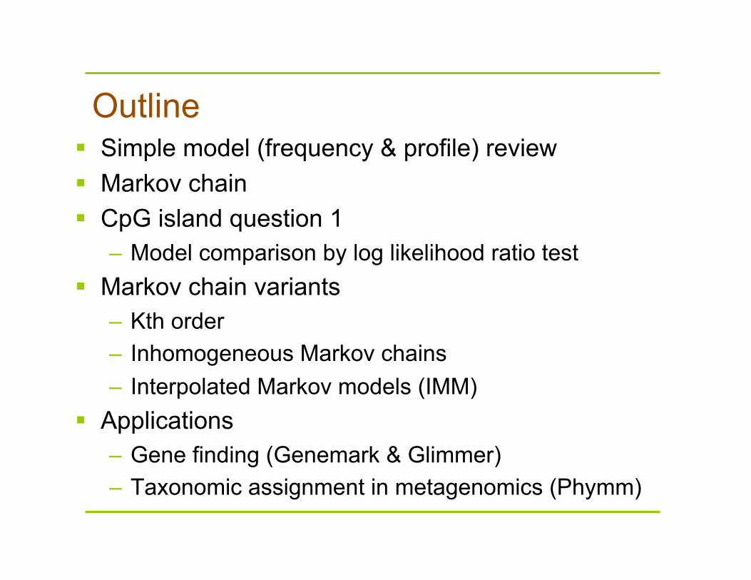
Outline   Simple model (frequency & profile) review   Markov chain   CpG island question 1

–  Model comparison by log likelihood ratio test   Markov chain variants

–  Kth order –  Inhomogeneous Markov chains –  Interpolated Markov models (IMM)

  Applications –  Gene finding (Genemark & Glimmer) –  Taxonomic assignment in metagenomics (Phymm)

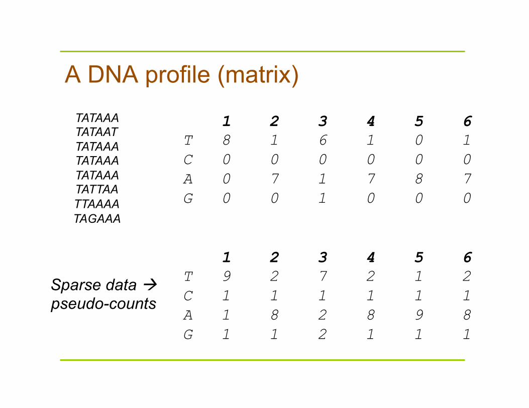
A DNA profile (matrix) TATAAA TATAAT TATAAA TATAAA TATAAA TATTAA TTAAAA TAGAAA

1 2 3 4 5 6 T 8 1 6 1 0 1 C 0 0 0 0 0 0 A 0 7 1 7 8 7 G 0 0 1 0 0 0

1 2 3 4 5 6 T 9 2 7 2 1 2 C 1 1 1 1 1 1 A 1 8 2 8 9 8 G 1 1 2 1 1 1

Sparse data pseudo-counts

Frequency & profile model

  Frequency model: the order of nucleotides in the training sequences is ignored;

  Profile model: the training sequences are aligned the order of nucleotides in the training sequences is fully preserved

  Markov chain model: orders are partially incorporated

Markov chain model   Sometimes we need to model

dependencies between adjacent positions in the sequence

–  There are certain regions in the genome, like TATA within the regulatory area, upstream a gene.

–  The pattern CG is less common than expected for random sampling.

  Such dependencies can be modeled by Markov chains.

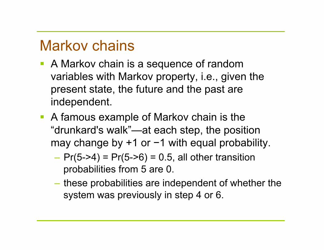
Markov chains   A Markov chain is a sequence of random

variables with Markov property, i.e., given the present state, the future and the past are independent.

  A famous example of Markov chain is the “drunkard's walk”—at each step, the position may change by +1 or −1 with equal probability. –  Pr(5->4) = Pr(5->6) = 0.5, all other transition

probabilities from 5 are 0. –  these probabilities are independent of whether the

system was previously in step 4 or 6.

1st order Markov chain

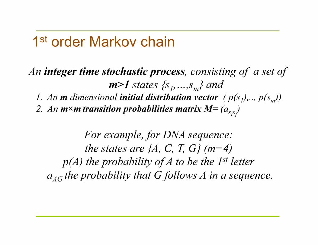
An integer time stochastic process, consisting of a set of m>1 states {s1,…,sm} and

1.  An m dimensional initial distribution vector ( p(s1),.., p(sm)) 2.  An m×m transition probabilities matrix M= (asisj)

For example, for DNA sequence: the states are {A, C, T, G} (m=4)

p(A) the probability of A to be the 1st letter aAG the probability that G follows A in a sequence.

1st order Markov chain

1 2 1 1 1 12

(( , ,... )) ( ) ( | )n

n i i i ii

p x x x p X x p X x X x− −=

= = = =∏

112

( )i i

n

x xi

p x a−

=

= ∏

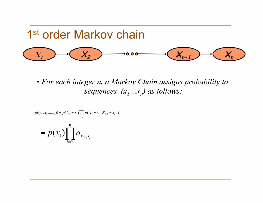
X1 X2 Xn-1 Xn

•  For each integer n, a Markov Chain assigns probability to sequences (x1…xn) as follows:

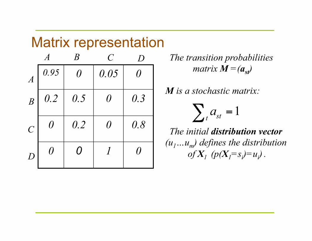
Matrix representation

1stta =∑

0 1 0 0

0.8 0 0.2 0

0.3 0 0.5 0.2

0 0.05 0 0.95 A B

B

A

C

C

D

D

M is a stochastic matrix:

The initial distribution vector (u1…um) defines the distribution

of X1 (p(X1=si)=ui) .

The transition probabilities matrix M =(ast)

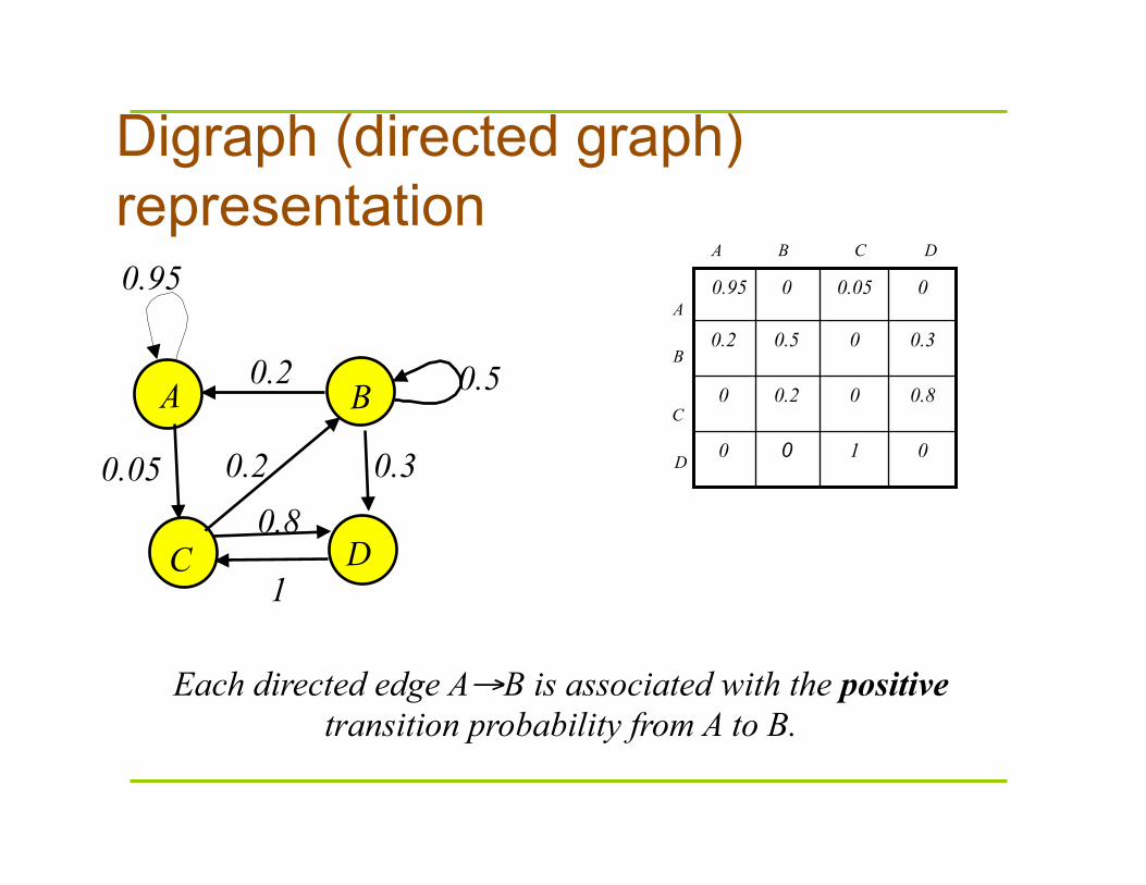
Digraph (directed graph) representation

Each directed edge A→B is associated with the positive transition probability from A to B.

A B

C D

0.2

0.3

0.5

0.05

0.95

0.2 0.8

1

0 1 0 0

0.8 0 0.2 0

0.3 0 0.5 0.2

0 0.05 0 0.95

A B

B

A

C

C

D

D

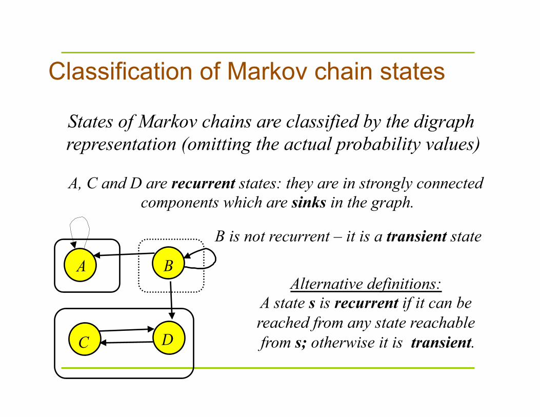
Classification of Markov chain states

A B

C D

States of Markov chains are classified by the digraph representation (omitting the actual probability values)

A, C and D are recurrent states: they are in strongly connected components which are sinks in the graph.

B is not recurrent – it is a transient state

Alternative definitions: A state s is recurrent if it can be reached from any state reachable from s; otherwise it is transient.

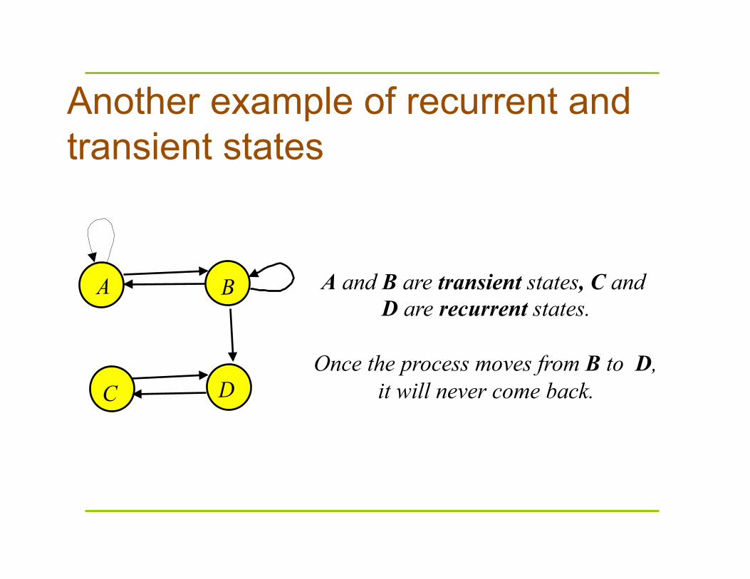
Another example of recurrent and transient states

A B

C D

A and B are transient states, C and D are recurrent states.

Once the process moves from B to D,

it will never come back.

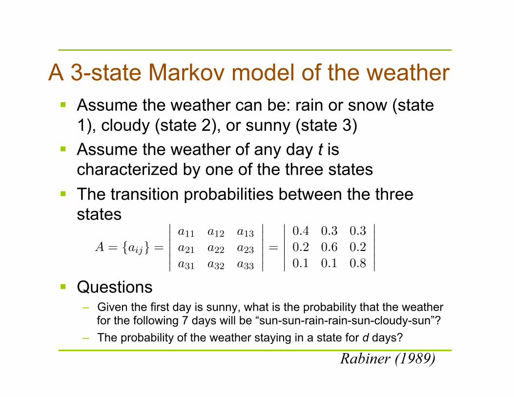
A 3-state Markov model of the weather   Assume the weather can be: rain or snow (state

1), cloudy (state 2), or sunny (state 3)   Assume the weather of any day t is

characterized by one of the three states   The transition probabilities between the three

states

  Questions

–  Given the first day is sunny, what is the probability that the weather for the following 7 days will be “sun-sun-rain-rain-sun-cloudy-sun”?

–  The probability of the weather staying in a state for d days?

Markov Models and Hidden Markov Models

Yuzhen Ye

December 26, 2012

1 Definition of HMM

The Hidden Markov Model is a finite set of states, each of which is associated with a(generally multidimensional) probability distribution (emission probabilities). Transitionsamong the states are governed by a set of probabilities called transition probabilities. Inparticular an outcome or observation can be generated, according to the associated prob-ability distribution. It is only the outcome, not the state visible to an external observerand therefore states are ”hidden” to the outside; hence the name Hidden Markov Model.

1.1 A simple 3-state Markov model of the weather

We assume that the weather can be characterized by three states: rain or snow (state 1),cloudy (state 2), and sunny (state 3), and the weather of any day t can be characterized bya single one of the three sates. The transition probabilities between the states is representedas a matrix A as,

A = {aij} =

������

a11 a12 a13

a21 a22 a23

a31 a32 a33

������=

������

0.4 0.3 0.30.2 0.6 0.20.1 0.1 0.8

������(1)

2 Assumptions in the theory of HMMs

2.1 The Markov assumption

The Markov assumption refers to the dependence of temporal states represented in thearchitecture. Under the Markov Assumption the values in any state are only influenced bythe values of the state that directly preceded it (or the next state is dependent only on thecurrent state). This is an important simplifying assumption which reduces the complexityof planning sequences of actions.

As given in the definition of HMMs, transition probabilities are defined as,

aij = p{qt + 1 = j|qt = i} (2)

1

Rabiner (1989)

CpG island modeling   In mammalian genomes, the dinucleotide CG

often transforms to (methyl-C)G which often subsequently mutates to TG.

  Hence CG appears less than expected from what is expected from the independent frequencies of C and G alone.

  Due to biological reasons, this process is sometimes suppressed in short stretches of genomes such as in the upstream regions of many genes.

  These areas are called CpG islands.

Questions about CpG islands We consider two questions (and some variants):

Question 1: Given a short stretch of genomic data, does

it come from a CpG island ?

Question 2: Given a long piece of genomic data, does it contain CpG islands in it, where, and how long?

We “solve” the first question by modeling sequences

with and without CpG islands as Markov Chains over the same states {A,C,G,T} but different transition

probabilities.

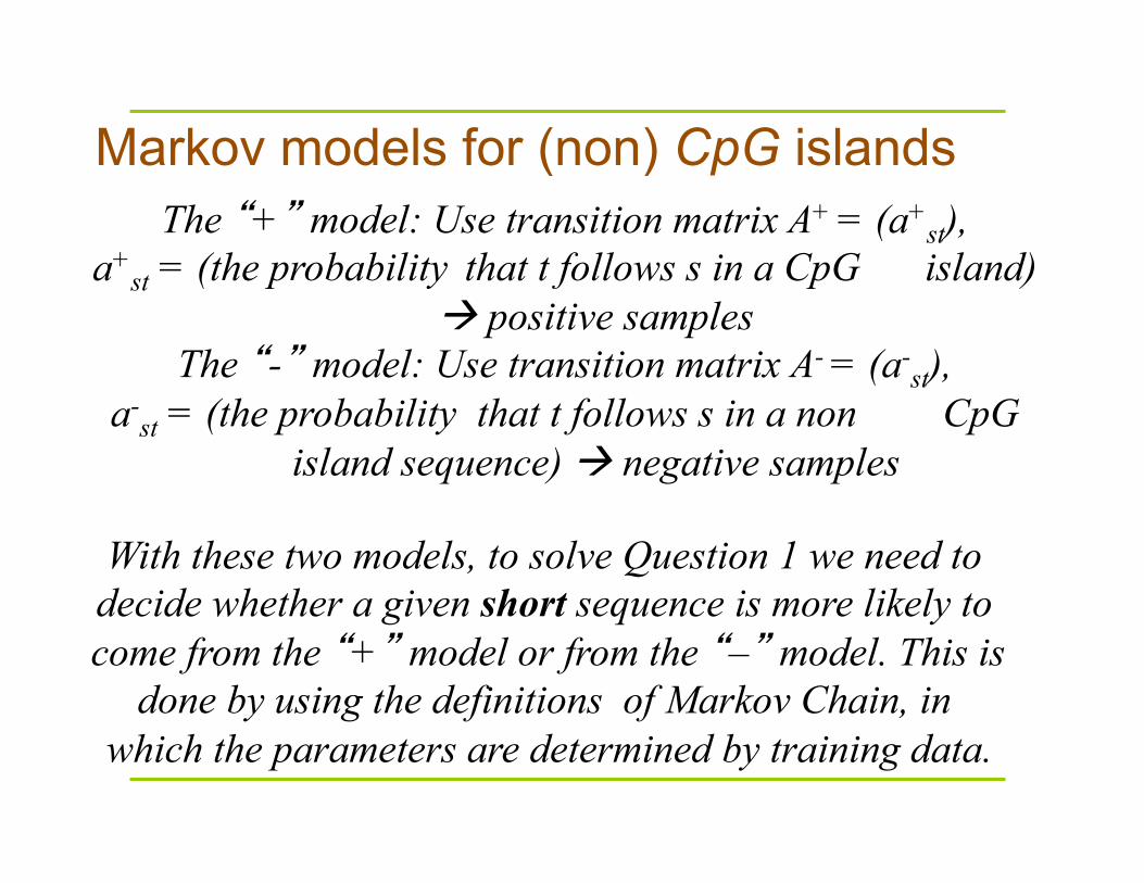
Markov models for (non) CpG islands

With these two models, to solve Question 1 we need to decide whether a given short sequence is more likely to come from the “+” model or from the “–” model. This is

done by using the definitions of Markov Chain, in which the parameters are determined by training data.

The “+” model: Use transition matrix A+ = (a+st),

a+st = (the probability that t follows s in a CpG island)

positive samples The “-” model: Use transition matrix A- = (a-

st), a-

st = (the probability that t follows s in a non CpG island sequence) negative samples

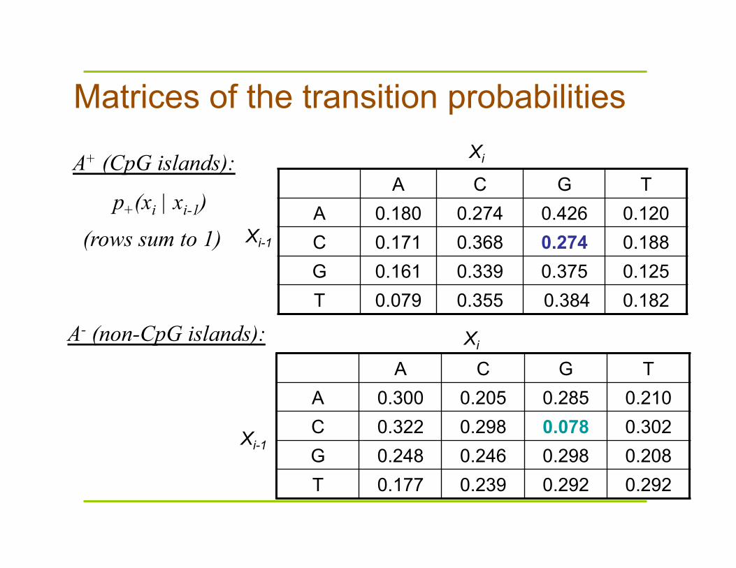
A+ (CpG islands):

Xi-1

Xi

Matrices of the transition probabilities

A C G T A 0.180 0.274 0.426 0.120 C 0.171 0.368 0.274 0.188 G 0.161 0.339 0.375 0.125 T 0.079 0.355 0.384 0.182

p+(xi | xi-1) (rows sum to 1)

Xi-1

Xi

A C G T A 0.300 0.205 0.285 0.210 C 0.322 0.298 0.078 0.302 G 0.248 0.246 0.298 0.208 T 0.177 0.239 0.292 0.292

A- (non-CpG islands):

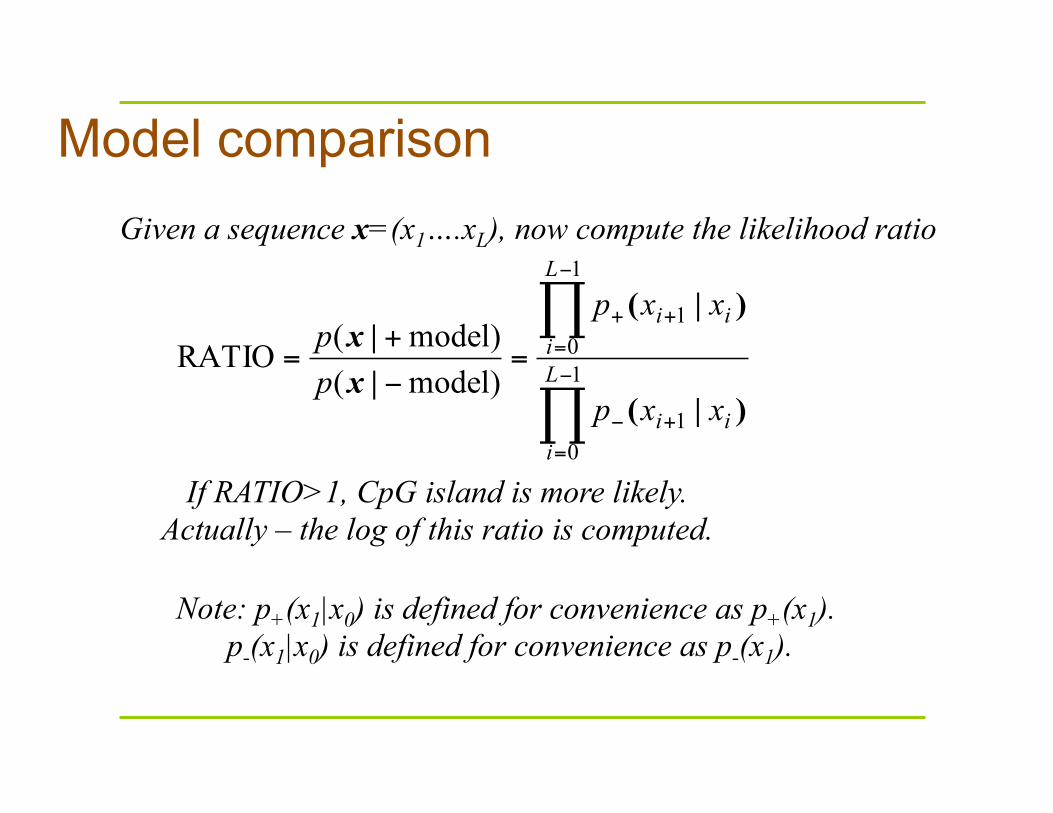
Model comparison Given a sequence x=(x1….xL), now compute the likelihood ratio

If RATIO>1, CpG island is more likely. Actually – the log of this ratio is computed.

∏

∏−

=+−

−

=++

=−

+= 1

01

1

01

model) (model) (RATIO L

iii

L

iii

xxp

xxp

pp

)|(

)|(

||xx

Note: p+(x1|x0) is defined for convenience as p+(x1). p-(x1|x0) is defined for convenience as p-(x1).

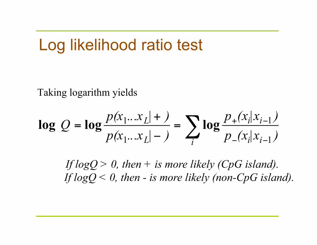
Log likelihood ratio test

Taking logarithm yields

If logQ > 0, then + is more likely (CpG island). If logQ < 0, then - is more likely (non-CpG island).

∑−−

−+=−

+=

i ii

ii

L

L

)|x(xp)|x(xp

)|...xp(x)|...xp(x Q

1

1

1

1 logloglog

A toy example

  Sequence: CGACTGAACCG

  P(CGACTGAACCG|+) = ?

  P(CGACTGAACCG|-) = ?

  Log likelihood ratio?

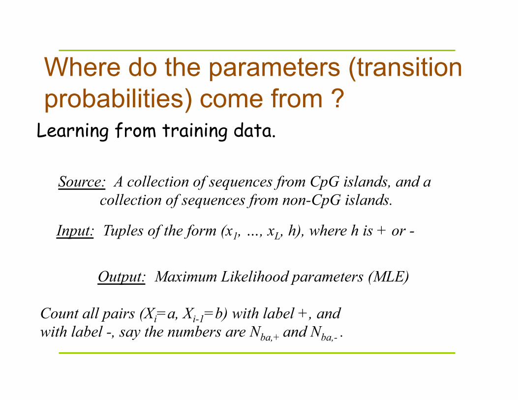
Where do the parameters (transition probabilities) come from ?

Learning from training data.

Source: A collection of sequences from CpG islands, and a collection of sequences from non-CpG islands.

Input: Tuples of the form (x1, …, xL, h), where h is + or -

Output: Maximum Likelihood parameters (MLE)

Count all pairs (Xi=a, Xi-1=b) with label +, and with label -, say the numbers are Nba,+ and Nba,- .

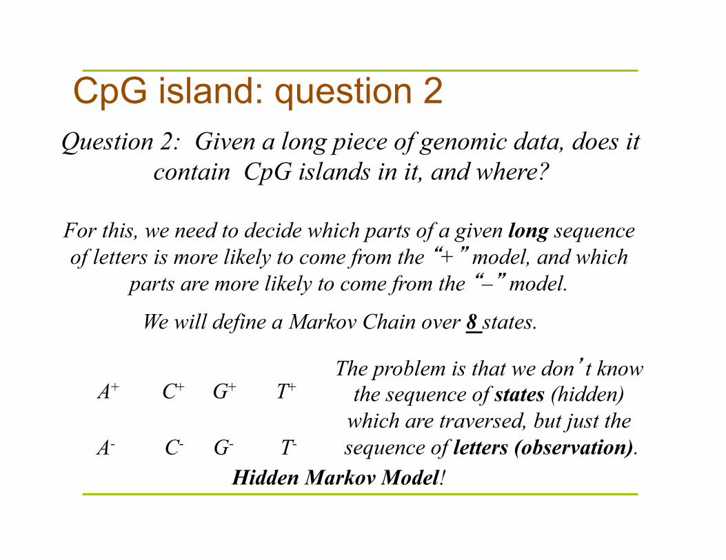
CpG island: question 2 Question 2: Given a long piece of genomic data, does it

contain CpG islands in it, and where?

For this, we need to decide which parts of a given long sequence of letters is more likely to come from the “+” model, and which

parts are more likely to come from the “–” model. We will define a Markov Chain over 8 states.

C+ T+ G+ A+

C- T- G- A-

The problem is that we don’t know the sequence of states (hidden)

which are traversed, but just the sequence of letters (observation).

Therefore we will use here Hidden Markov Model!

Hidden Markov Model!

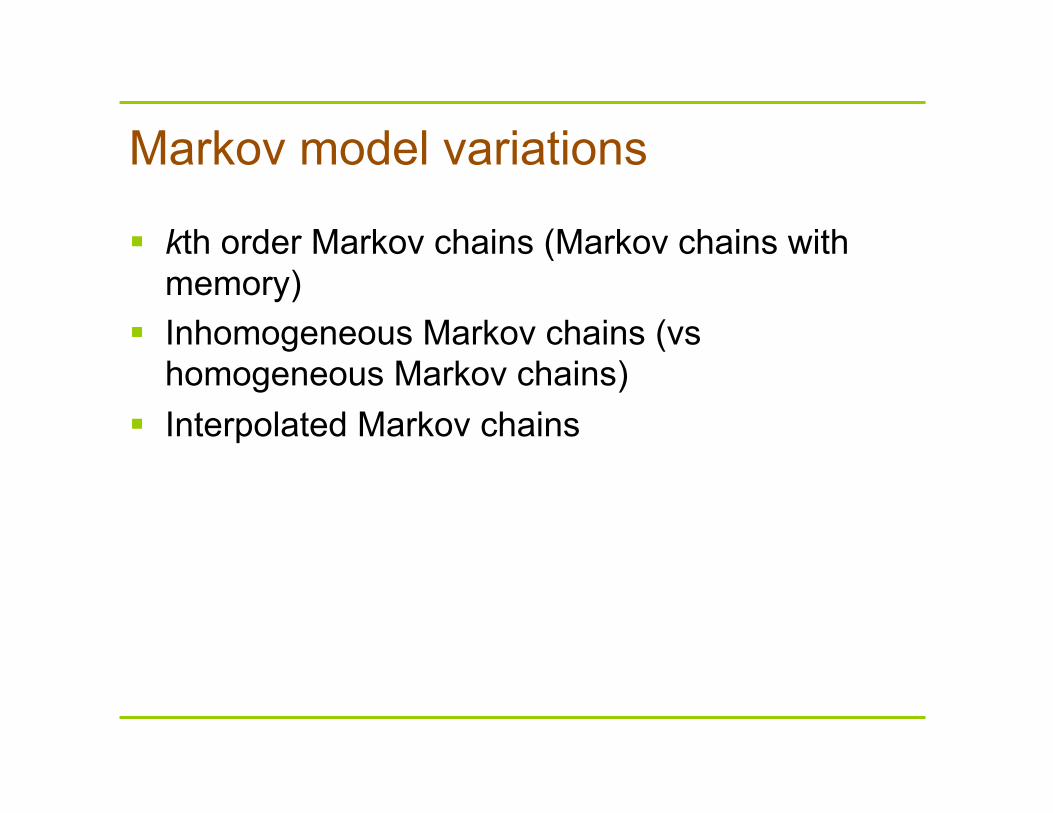
Markov model variations

  kth order Markov chains (Markov chains with memory)

  Inhomogeneous Markov chains (vs homogeneous Markov chains)

  Interpolated Markov chains

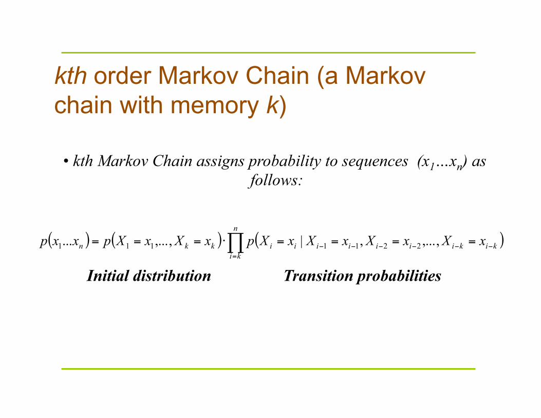
kth order Markov Chain (a Markov chain with memory k)

( ) ( ) ( )∏=

−−−−−− ====⋅===n

kikikiiiiiiikkn xXxXxXxXpxXxXpxxp ,...,,|,...,... 2211111

•  kth Markov Chain assigns probability to sequences (x1…xn) as follows:

Initial distribution Transition probabilities

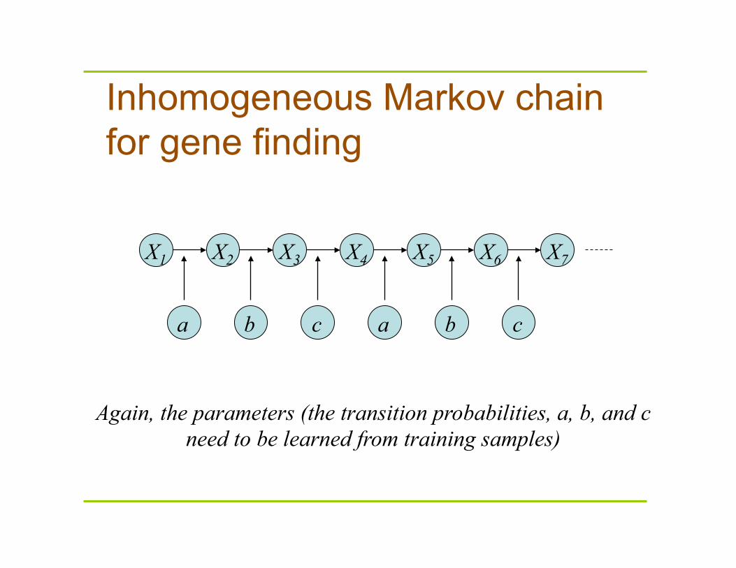
Inhomogeneous Markov chain for gene finding

X1 X2 X3 X4 X5 X6 X7

a a b b c c

Again, the parameters (the transition probabilities, a, b, and c need to be learned from training samples)

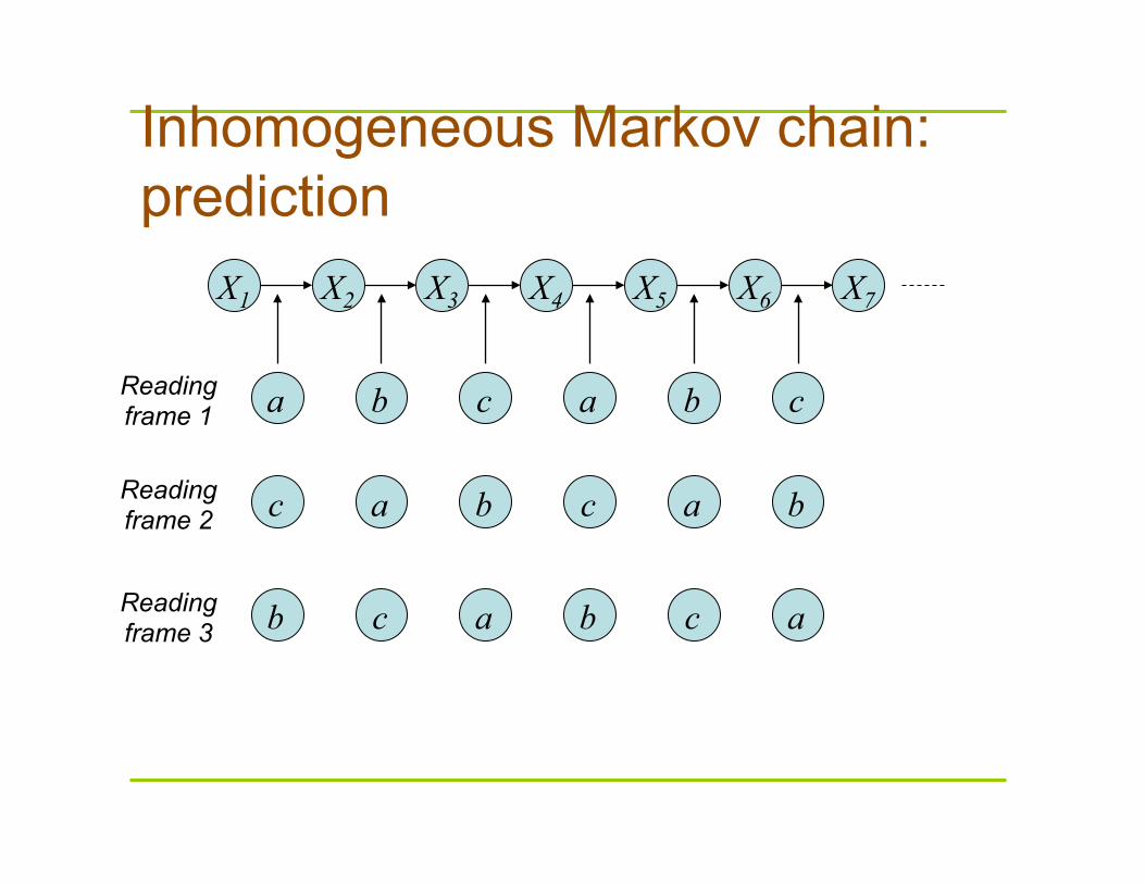
Inhomogeneous Markov chain: prediction

X1 X2 X3 X4 X5 X6 X7

a a b b c c Reading frame 1

a a b b c c Reading frame 2

a a b b c c Reading frame 3

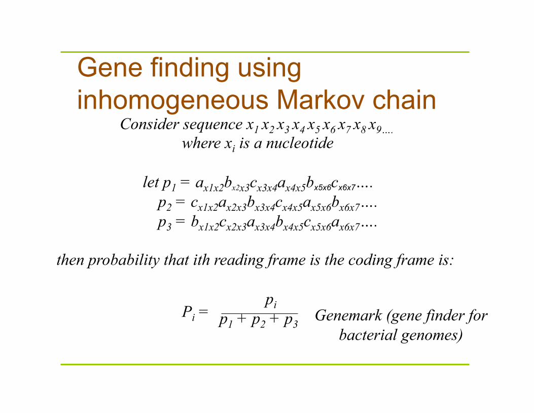
Gene finding using inhomogeneous Markov chain

Consider sequence x1 x2 x3 x4 x5 x6 x7 x8 x9…. where xi is a nucleotide

let p1 = ax1x2bx2x3cx3x4ax4x5bx5x6cx6x7….

p2 = cx1x2ax2x3bx3x4cx4x5ax5x6bx6x7…. p3 = bx1x2cx2x3ax3x4bx4x5cx5x6ax6x7….

then probability that ith reading frame is the coding frame is:

pi

p1 + p2 + p3

Genemark (gene finder for

bacterial genomes) Pi =

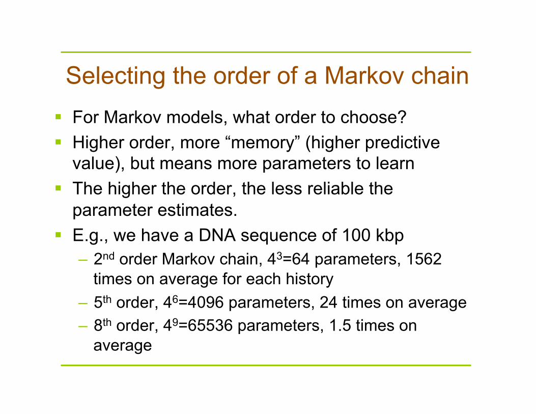
Selecting the order of a Markov chain   For Markov models, what order to choose?   Higher order, more “memory” (higher predictive

value), but means more parameters to learn   The higher the order, the less reliable the

parameter estimates.   E.g., we have a DNA sequence of 100 kbp

–  2nd order Markov chain, 43=64 parameters, 1562 times on average for each history

–  5th order, 46=4096 parameters, 24 times on average –  8th order, 49=65536 parameters, 1.5 times on

average

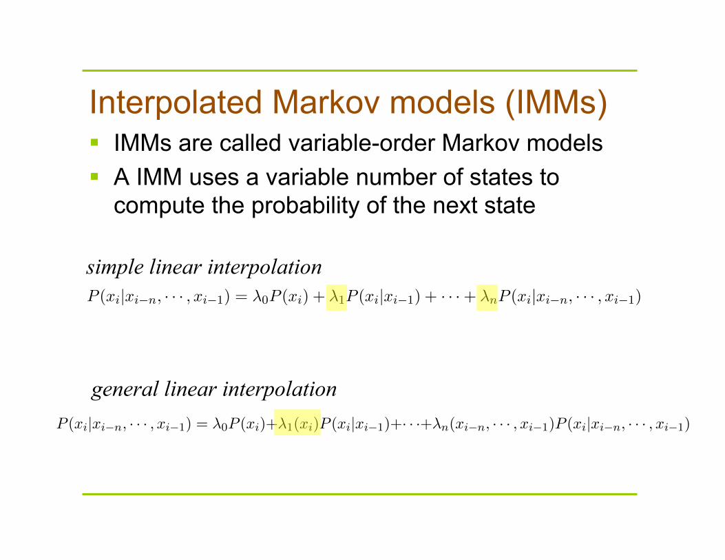
Interpolated Markov models (IMMs)   IMMs are called variable-order Markov models   A IMM uses a variable number of states to

compute the probability of the next state

simple linear interpolation

general linear interpolation

Markov Models and Hidden Markov Models

Yuzhen Ye

January 4, 2013

1 Definition of Markov model

1.1 Markov chain

A Markov chain is a sequence of random variables with Markov property, i.e., given thepresent state, the future and the past are independent.

1.2 Interpolated Markov models (IMMs)

IMMs are a form of Markov model that use variable states to calculate the probability.Simple linear interpolation

P (xi|xi�n, · · · , xi�1) = �0P (xi) + �1P (xi|xi�1) + · · ·+ �nP (xi|xi�n, · · · , xi�1) (1)

General linear interpolation

P (xi|xi�n, · · · , xi�1) = �0P (xi)+�1(xi)P (xi|xi�1)+· · ·+�n(xi�n, · · · , xi�1)P (xi|xi�n, · · · , xi�1)(2)

2 Definition of HMM

The Hidden Markov Model is a finite set of states, each of which is associated with a(generally multidimensional) probability distribution (emission probabilities). Transitionsamong the states are governed by a set of probabilities called transition probabilities. Inparticular an outcome or observation can be generated, according to the associated prob-ability distribution. It is only the outcome, not the state visible to an external observerand therefore states are ”hidden” to the outside; hence the name Hidden Markov Model.

2.1 A simple 3-state Markov model of the weather

We assume that the weather can be characterized by three states: rain or snow (state 1),cloudy (state 2), and sunny (state 3), and the weather of any day t can be characterized by

1

Markov Models and Hidden Markov Models

Yuzhen Ye

January 4, 2013

1 Definition of Markov model

1.1 Markov chain

A Markov chain is a sequence of random variables with Markov property, i.e., given thepresent state, the future and the past are independent.

1.2 Interpolated Markov models (IMMs)

IMMs are a form of Markov model that use variable states to calculate the probability.Simple linear interpolation

P (xi|xi�n, · · · , xi�1) = �0P (xi) + �1P (xi|xi�1) + · · ·+ �nP (xi|xi�n, · · · , xi�1) (1)

General linear interpolation

P (xi|xi�n, · · · , xi�1) = �0P (xi)+�1(xi)P (xi|xi�1)+· · ·+�n(xi�n, · · · , xi�1)P (xi|xi�n, · · · , xi�1)(2)

2 Definition of HMM

The Hidden Markov Model is a finite set of states, each of which is associated with a(generally multidimensional) probability distribution (emission probabilities). Transitionsamong the states are governed by a set of probabilities called transition probabilities. Inparticular an outcome or observation can be generated, according to the associated prob-ability distribution. It is only the outcome, not the state visible to an external observerand therefore states are ”hidden” to the outside; hence the name Hidden Markov Model.

2.1 A simple 3-state Markov model of the weather

We assume that the weather can be characterized by three states: rain or snow (state 1),cloudy (state 2), and sunny (state 3), and the weather of any day t can be characterized by

1

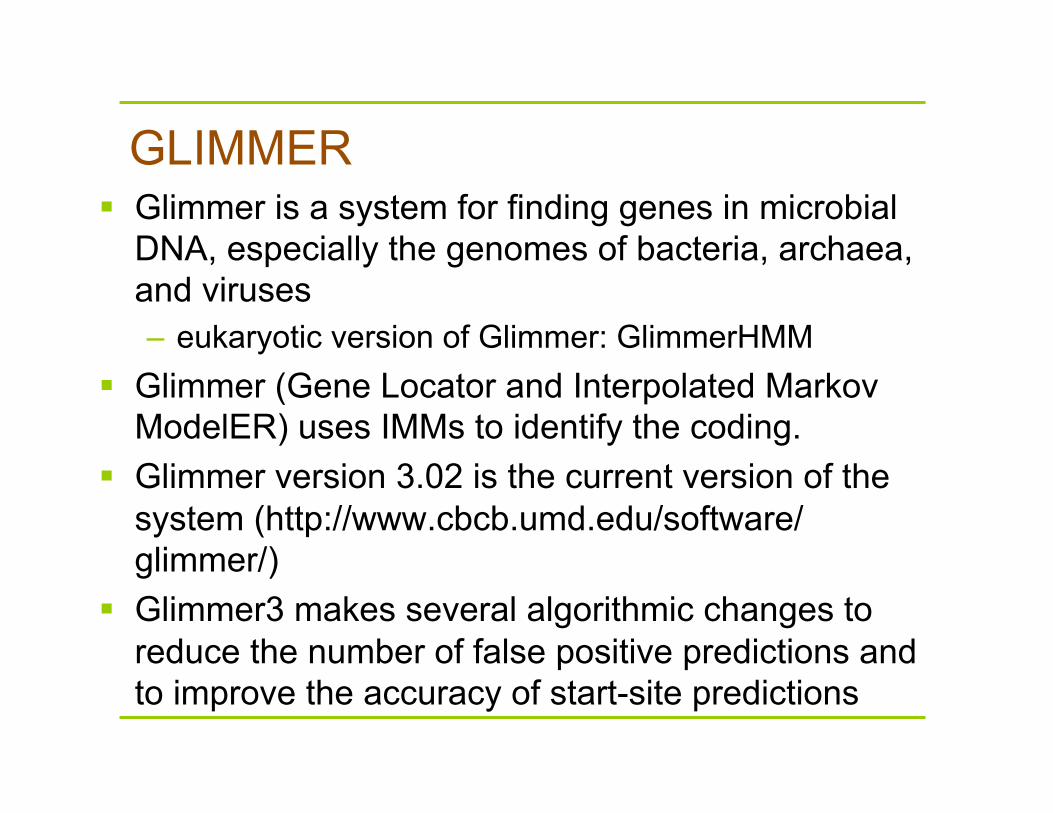
GLIMMER   Glimmer is a system for finding genes in microbial

DNA, especially the genomes of bacteria, archaea, and viruses –  eukaryotic version of Glimmer: GlimmerHMM

  Glimmer (Gene Locator and Interpolated Markov ModelER) uses IMMs to identify the coding.

  Glimmer version 3.02 is the current version of the system (http://www.cbcb.umd.edu/software/glimmer/)

  Glimmer3 makes several algorithmic changes to reduce the number of false positive predictions and to improve the accuracy of start-site predictions

IMM in GLIMMER   A linear combination of 8 different Markov chains,

from 1st through 8th-order, weighting each model according to its predictive power.

  Glimmer uses 3-periodic nonhomogenous Markov models in its IMMs.

  Score of a sequence is the product of interpolated probabilities of bases in the sequence

  IMM training –  Longer context is always better; only reason not

to use it is undersampling in training data. –  If sequence occurs frequently enough in training

data, use it, i.e., λ = 1 –  Otherwise, use frequency and χ2 significance to

set λ.

Clustering metagenomic sequences with IMMs   IMMs are used to classify metagenomic

sequences based on patterns of DNA distinct to a clade (a species, genus, or higher-level phylogenetic group).

  During training, the IMM algorithm constructs probability distributions representing observed patterns of nucleotides that characterize each species.

  Nat Methods 2009, 6(9):673-676