Markov Localization for Mobile Robots in Dynamic …biorobotics.ri.cmu.edu/papers/sbp_papers/integrated4/burgard_bayes... · Localization, that is the estimation of a robot's location

Next: Introduction

Journal of Artificial Intelligence Research 11 (1999), pp. 391-427. Submitted 1/99; published 11/99. © 1999 AI Access Foundation and Morgan Kaufmann Publishers. All rights reserved.

Markov Localization for Mobile Robots in Dynamic Environments

Dieter FoxComputer Science Department and Robotics Institute

Carnegie Mellon UniversityPittsburgh, PA 15213-3891

Wolfram BurgardDepartment of Computer Science

University of FreiburgD-79110 Freiburg, Germany

Sebastian Thrun Computer Science Department and Robotics Institute

Carnegie Mellon UniversityPittsburgh, PA 15213-3891

Abstract:

Localization, that is the estimation of a robot's location from sensor data, is a fundamental problem in mobilerobotics. This papers presents a version of Markov localization which provides accurate position estimates andwhich is tailored towards dynamic environments. The key idea of Markov localization is to maintain a probabilitydensity over the space of all locations of a robot in its environment. Our approach represents this space metrically,using a fine-grained grid to approximate densities. It is able to globally localize the robot from scratch and torecover from localization failures. It is robust to approximate models of the environment (such as occupancy gridmaps) and noisy sensors (such as ultrasound sensors). Our approach also includes a filtering technique whichallows a mobile robot to reliably estimate its position even in densely populated environments in which crowds ofpeople block the robot's sensors for extended periods of time. The method described here has been implementedand tested in several real-world applications of mobile robots, including the deployments of two mobile robots asinteractive museum tour-guides.

Introduction Markov Localization

The Basic Idea Basic Notation Recursive Localization

1 of 2 12/10/00 10:59 AM

Markov Localization for Mobile Robots in Dynaic Environments http://www.cs.cmu.edu/afs/cs/project/jair/pub/volume11/fox99a-html/jair-localize.html

The Markov Localization Algorithm Implementations of Markov Localization

Metric Markov Localization for Dynamic Environments The Action Model The Perception Model for Proximity Sensors Filtering Techniques for Dynamic Environments

The Entropy Filter The Distance Filter

Grid-based Representation of the State Space Pre-Computation of the Sensor Model Selective Update

Experimental Results Long-term Experiments in Dynamic Environments

Datasets Tracking the Robot's Position Recovery from Extreme Localization Failures

Localization in Incomplete Maps Localization in Occupancy Grid Maps Using Sonar Precision and Performance

Related Work Discussion References About this document ...

Dieter Fox Fri Nov 19 14:29:33 MET 1999

2 of 2 12/10/00 10:59 AM

Markov Localization for Mobile Robots in Dynaic Environments http://www.cs.cmu.edu/afs/cs/project/jair/pub/volume11/fox99a-html/jair-localize.html

Next: Markov Localization Up: Markov Localization for Mobile Previous: Markov Localization for Mobile

Introduction

Robot localization has been recognized as one of the most fundamental problems in mobile robotics [Cox &Wilfong1990, Borenstein et al. 1996]. The aim of localization is to estimate the postition of a robot in itsenvironment, given a map of the environment and sensor data. Most successful mobile robot systems to date utilizelocalization, as knowledge of the robot's position is essential for a broad range of mobile robot tasks.

Localization--often referred to as position estimation or position control--is currently a highly active field ofresearch, as a recent book by Borenstein and colleagues [Borenstein et al. 1996] suggests. The localizationtechniques developed so far can be distinguished according to the type of problem they attack. Tracking or localtechniques aim at compensating odometric errors occurring during robot navigation. They require, however, thatthe initial location of the robot is (approximately) known and they typically cannot recover if they lose track of therobot's position (within certain bounds). Another family of approaches is called global techniques. These aredesigned to estimate the position of the robot even under global uncertainty. Techniques of this type solve theso-called wake-up robot problem, in that they can localize a robot without any prior knowledge about itsposition. They furthermore can handle the kidnapped robot problem, in which a robot is carried to an arbitrarylocation during it's operation. Please note that the wake-up problem is the special case of the kidnapped robotproblem in which the robot is told that it has been carried away. Global localization techniques are more powerfulthan local ones. They typically can cope with situations in which the robot is likely to experience serious positioningerrors.

In this paper we present a metric variant of Markov localization, a technique to globally estimate the position of arobot in its environment. Markov localization uses a probabilistic framework to maintain a position probabilitydensity over the whole set of possible robot poses. Such a density can have arbitrary forms representing variouskinds of information about the robot's position. For example, the robot can start with a uniform distributionrepresenting that it is completely uncertain about its position. It furthermore can contain multiple modes in the caseof ambiguous situations. In the usual case, in which the robot is highly certain about its position, it consists of aunimodal distribution centered around the true position of the robot. Based on the probabilistic nature of theapproach and the representation, Markov localization can globally estimate the position of the robot, it can dealwith ambiguous situations, and it can re-localize the robot in the case of localization failures. These properties arebasic preconditions for truly autonomous robots designed to operate over long periods of time.

Our method uses a fine-grained and metric discretization of the state space. This approach has several advantagesover previous ones, which predominately used Gaussians or coarse-grained, topological representations forapproximating a robot's belief. First, it provides more accurate position estimates, which are required in manymobile robot tasks (e.g., tasks involving mobile manipulation). Second, it can incorporate raw sensory input suchas a single beam of an ultrasound sensor. Most previous approaches to Markov localization, in contrast, screensensor data for the presence or absence of landmarks, and they are prone to fail if the environment does not alignwell with the underlying assumptions (e.g., if it does not contain any of the required landmarks).

Most importantly, however, previous Markov localization techniques assumed that the environment is static.Therefore, they typically fail in highly dynamic environments, such as public places where crowds of people may

1 of 2 12/10/00 11:00 AM

Introduction http://www.cs.cmu.edu/afs/cs/project/jair/pub/volume11/fox99a-html/node1.html

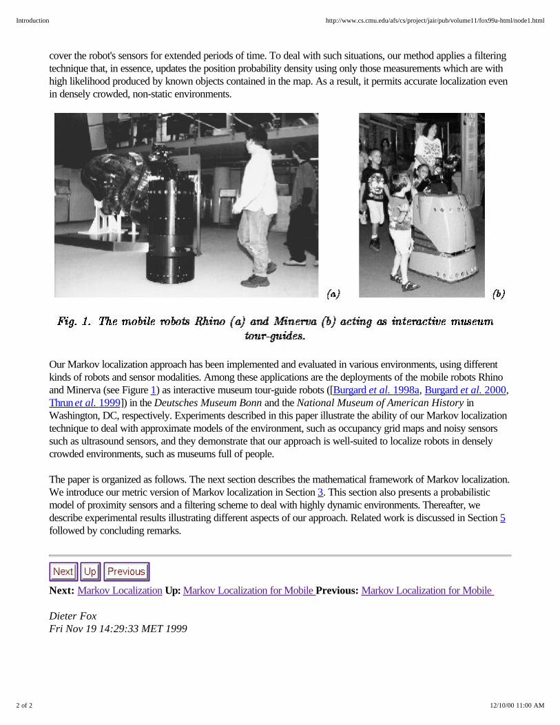
cover the robot's sensors for extended periods of time. To deal with such situations, our method applies a filteringtechnique that, in essence, updates the position probability density using only those measurements which are withhigh likelihood produced by known objects contained in the map. As a result, it permits accurate localization evenin densely crowded, non-static environments.

Our Markov localization approach has been implemented and evaluated in various environments, using differentkinds of robots and sensor modalities. Among these applications are the deployments of the mobile robots Rhinoand Minerva (see Figure 1) as interactive museum tour-guide robots ([Burgard et al. 1998a, Burgard et al. 2000,Thrun et al. 1999]) in the Deutsches Museum Bonn and the National Museum of American History inWashington, DC, respectively. Experiments described in this paper illustrate the ability of our Markov localizationtechnique to deal with approximate models of the environment, such as occupancy grid maps and noisy sensorssuch as ultrasound sensors, and they demonstrate that our approach is well-suited to localize robots in denselycrowded environments, such as museums full of people.

The paper is organized as follows. The next section describes the mathematical framework of Markov localization.We introduce our metric version of Markov localization in Section 3. This section also presents a probabilisticmodel of proximity sensors and a filtering scheme to deal with highly dynamic environments. Thereafter, wedescribe experimental results illustrating different aspects of our approach. Related work is discussed in Section 5followed by concluding remarks.

Next: Markov Localization Up: Markov Localization for Mobile Previous: Markov Localization for Mobile


2 of 2 12/10/00 11:00 AM

Introduction http://www.cs.cmu.edu/afs/cs/project/jair/pub/volume11/fox99a-html/node1.html

Next: The Basic Idea Up: Markov Localization for Mobile Previous: Introduction

Markov Localization

To introduce the major concepts, we will begin with an intuitive description of Markov localization, followed by amathematical derivation of the algorithm. The reader may notice that Markov localization is a special case ofprobabilistic state estimation, applied to mobile robot localization (see also [Russell & Norvig1995, Fox1998,Koenig & Simmons1998]).

For clarity of the presentation, we will initially make the restrictive assumption that the environment is static. Thisassumption, called Markov assumption, is commonly made in the robotics literature. It postulates that the robot'slocation is the only state in the environment which systematically affects sensor readings. The Markov assumptionis violated if robots share the same environment with people. Further below, in Section 3.3, we will side-step thisassumption and present a Markov localization algorithm that works well even in highly dynamic environments, e.g.,museums full of people.

The Basic Idea Basic Notation Recursive Localization The Markov Localization Algorithm Implementations of Markov Localization


1 of 1 12/10/00 11:17 AM

Markov Localization http://www.cs.cmu.edu/afs/cs/project/jair/pub/volume11/fox99a-html/node2.html

Next: Basic Notation Up: Markov Localization Previous: Markov Localization

The Basic Idea

Markov localization addresses the problem of state estimation from sensor data. Markov localization is aprobabilistic algorithm: Instead of maintaining a single hypothesis as to where in the world a robot might be,Markov localization maintains a probability distribution over the space of all such hypotheses. The probabilisticrepresentation allows it to weigh these different hypotheses in a mathematically sound way.

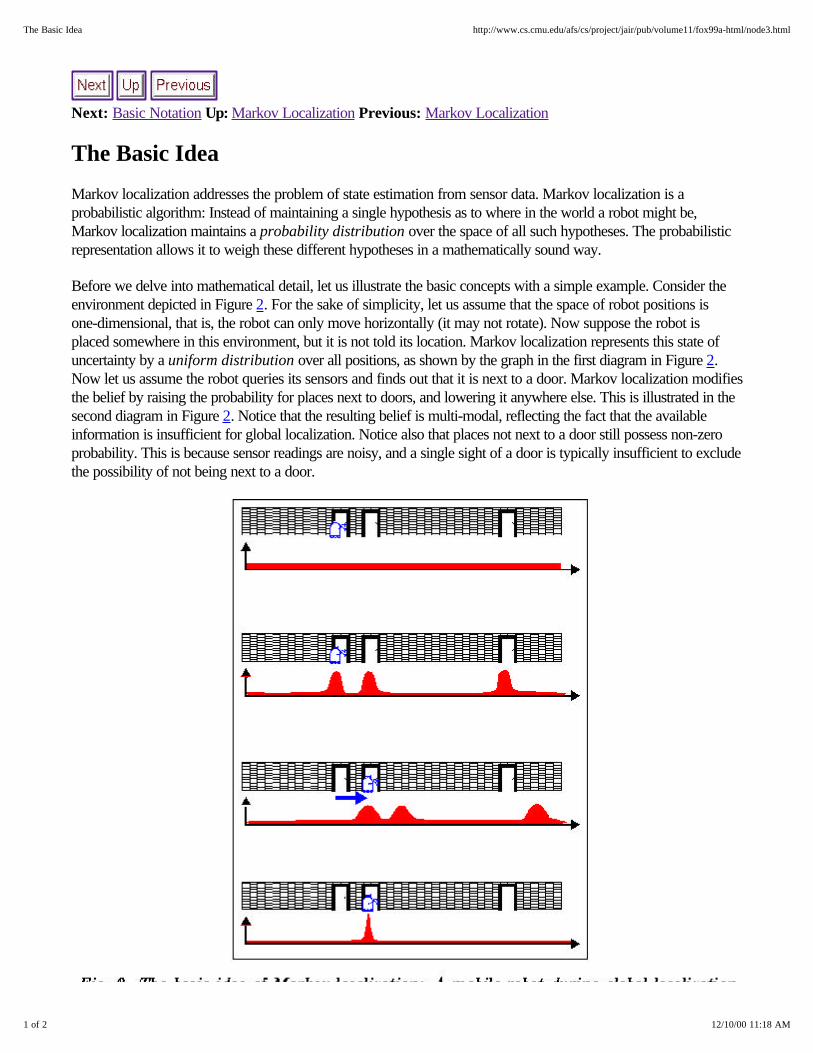
Before we delve into mathematical detail, let us illustrate the basic concepts with a simple example. Consider theenvironment depicted in Figure 2. For the sake of simplicity, let us assume that the space of robot positions isone-dimensional, that is, the robot can only move horizontally (it may not rotate). Now suppose the robot isplaced somewhere in this environment, but it is not told its location. Markov localization represents this state ofuncertainty by a uniform distribution over all positions, as shown by the graph in the first diagram in Figure 2.Now let us assume the robot queries its sensors and finds out that it is next to a door. Markov localization modifiesthe belief by raising the probability for places next to doors, and lowering it anywhere else. This is illustrated in thesecond diagram in Figure 2. Notice that the resulting belief is multi-modal, reflecting the fact that the availableinformation is insufficient for global localization. Notice also that places not next to a door still possess non-zeroprobability. This is because sensor readings are noisy, and a single sight of a door is typically insufficient to excludethe possibility of not being next to a door.

1 of 2 12/10/00 11:18 AM

The Basic Idea http://www.cs.cmu.edu/afs/cs/project/jair/pub/volume11/fox99a-html/node3.html

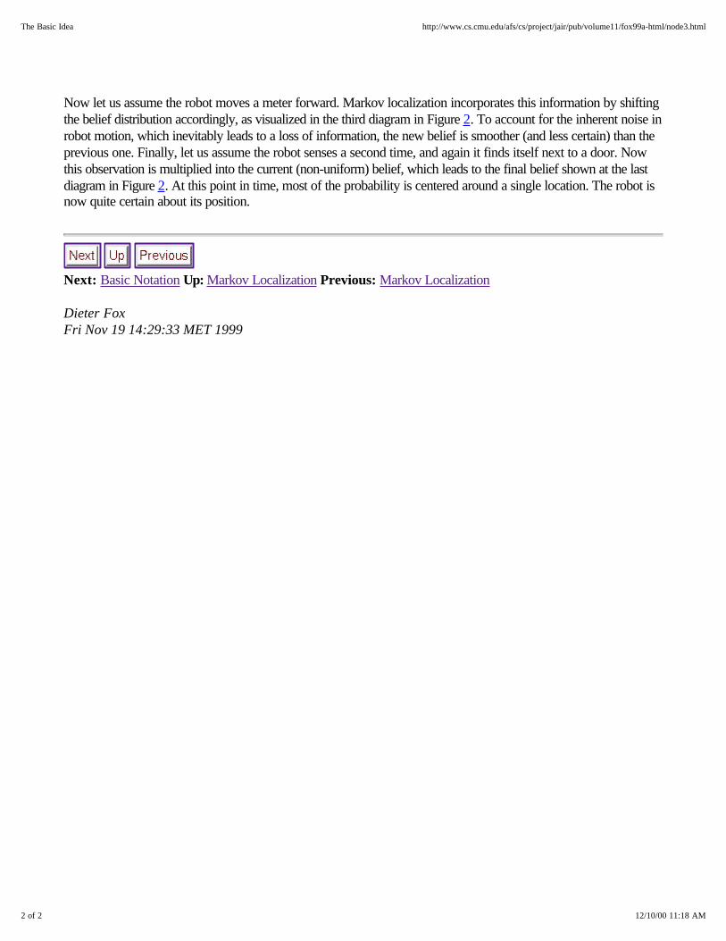
Now let us assume the robot moves a meter forward. Markov localization incorporates this information by shiftingthe belief distribution accordingly, as visualized in the third diagram in Figure 2. To account for the inherent noise inrobot motion, which inevitably leads to a loss of information, the new belief is smoother (and less certain) than theprevious one. Finally, let us assume the robot senses a second time, and again it finds itself next to a door. Nowthis observation is multiplied into the current (non-uniform) belief, which leads to the final belief shown at the lastdiagram in Figure 2. At this point in time, most of the probability is centered around a single location. The robot isnow quite certain about its position.

Next: Basic Notation Up: Markov Localization Previous: Markov Localization


2 of 2 12/10/00 11:18 AM

The Basic Idea http://www.cs.cmu.edu/afs/cs/project/jair/pub/volume11/fox99a-html/node3.html

Next: Recursive Localization Up: Markov Localization Previous: The Basic Idea

Basic Notation

To make this more formal, let us denote the position (or: location) of a mobile robot by a three-dimensionalvariable , comprising its x-y coordinates (in some Cartesian coordinate system) and its heading

direction . Let denote the robot's true location at time t, and denote the corresponding random variable.

Throughout this paper, we will use the terms position and location interchangeably.

Typically, the robot does not know its exact position. Instead, it carries a belief as to where it might be. Let denote the robot's position belief at time t. is a probability distribution over the space of

positions. For example, is the probability (density) that the robot assigns to the possibility that its

location at time t is l. The belief is updated in response to two different types of events: The arrival of ameasurement through the robot's environment sensors (e.g., a camera image, a sonar scan), and the arrival of anodometry reading (e.g., wheel revolution count). Let us denote environment sensor measurements by s andodometry measurements by a, and the corresponding random variables by S and A, respectively.

The robot perceives a stream of measurements, sensor measurements s and odometry readings a. Let

denote the stream of measurements, where each (with ) either is a sensor measurement or an

odometry reading. The variable t indexes the data, and T is the most recently collected data item (one might thinkof t as ``time''). The set d, which comprises all available sensor data, will be referred to as the data.


1 of 1 12/10/00 11:19 AM

Basic Notation http://www.cs.cmu.edu/afs/cs/project/jair/pub/volume11/fox99a-html/node4.html

Next: The Markov Localization Algorithm Up: Markov Localization Previous: Basic Notation

Recursive Localization

Markov localization estimates the posterior distribution over conditioned on all available data, that is

Before deriving incremental update equations for this posterior, let us briefly make explicit the key assumptionunderlying our derivation, called the Markov assumption. The Markov assumption, sometimes referred to asstatic world assumption, specifies that if one knows the robot's location , future measurements are independent

of past ones (and vice versa):

In other words, we assume that the robot's location is the only state in the environment, and knowing it is all oneneeds to know about the past to predict future data. This assumption is clearly inaccurate if the environmentcontains moving (and measurable) objects other than the robot itself. Further below, in Section 3.3, we will extendthe basic paradigm to non-Markovian environments, effectively devising a localization algorithm that works well ina broad range of dynamic environments. For now, however, we will adhere to the Markov assumption, to facilitatethe derivation of the basic algorithm.

When computing , we distinguish two cases, depending on whether the most recent data item

is a sensor measurement or an odometry reading.

Case 1: The most recent data item is a sensor measurement .

Here

Bayes rule suggests that this term can be transformed to

which, because of our Markov assumption, can be simplified to:

1 of 3 12/10/00 11:23 AM

Recursive Localization http://www.cs.cmu.edu/afs/cs/project/jair/pub/volume11/fox99a-html/node5.html

We also observe that the denominator can be replaced by a constant , since it does not depend on . Thus,

we have

The reader may notice the incremental nature of Equation (7): If we write

to denote the robot's belief Equation (7) becomes

In this equation we replaced the term by based on the assumption that it is

independent of the time.

Case 2: The most recent data item is an odometry reading: .

Here we compute using the Theorem of Total Probability:

Consider the first term on the right-hand side. Our Markov assumption suggests that

The second term on the right-hand side of Equation (10) can also be simplified by observing that does notcarry any information about the position :

Substituting 12 and 14 back into Equation (10) gives us the desired result

Notice that Equation (15) is, too, of an incremental form. With our definition of belief above, we have

2 of 3 12/10/00 11:23 AM


Please note that we used instead of since we assume that it does

not change over time.

Next: The Markov Localization Algorithm Up: Markov Localization Previous: Basic Notation


3 of 3 12/10/00 11:23 AM


Next: Implementations of Markov Localization Up: Markov Localization Previous: Recursive Localization

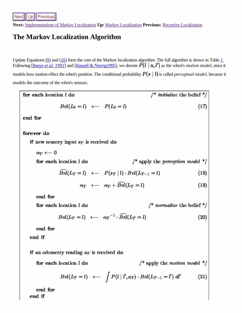
The Markov Localization Algorithm

Update Equations (9) and (16) form the core of the Markov localization algorithm. The full algorithm is shown in Table 1.Following [Basye et al. 1992] and [Russell & Norvig1995], we denote as the robot's motion model, since it

models how motion effect the robot's position. The conditional probability is called perceptual model, because it

models the outcome of the robot's sensors.

In the Markov localization algorithm , which initializes the belief , reflects the prior knowledge about

the starting position of the robot. This distribution can be initialized arbitrarily, but in practice two cases prevail: If theposition of the robot relative to its map is entirely unknown, is usually uniformly distributed. If the initial position of

the robot is approximately known, then is typically a narrow Gaussian distribution centered at the robot's position.


Next: Metric Markov Localization for Up: Markov Localization Previous: The Markov Localization Algorithm

Implementations of Markov Localization

The reader may notice that the principle of Markov localization leaves open

1. how the robot's belief Bel(L) is represented and2. how the conditional probabilities and are computed.

Accordingly, existing approaches to Markov localization mainly differ in the representation of the state space and thecomputation of the perceptual model. In this section we will briefly discuss different implementations of Markov localizationfocusing on these two topics (see Section 5 for a more detailed discussion of related work).

1. State Space Representations: A very common approach for the representation of the robots belief Bel(L) is basedon Kalman filtering [Kalman1960, Smith et al. 1990] which rests on the restrictive assumption that the position of therobot can be modeled by a unimodal Gaussian distribution. Existing implementations [Leonard &Durrant-Whyte1992, Schiele & Crowley1994, Gutmann & Schlegel1996, Arras & Vestli1998] have proven to berobust and accurate for keeping track of the robot's position. Because of the restrictive assumption of a Gaussiandistribution these techniques lack the ability to represent situations in which the position of the robot maintainsmultiple, distinct beliefs (c.f. 2). As a result, localization approaches using Kalman filters typically require that thestarting position of the robot is known and are not able to re-localize the robot in the case of localization failures.Additionally, Kalman filters rely on sensor models that generate estimates with Gaussian uncertainty. This assumption,unfortunately, is not met in all situations (see for example [Dellaert et al. 1999]).

To overcome these limitations, different approaches have used increasingly richer schemes to represent uncertainty inthe robot's position, moving beyond the Gaussian density assumption inherent in the vanilla Kalman filter.[Nourbakhsh et al. 1995, Simmons & Koenig1995, Kaelbling et al. 1996] use Markov localization forlandmark-based corridor navigation and the state space is organized according to the coarse, topological structure ofthe environment and with generally only four possible orientations of the robot. These approaches can, in principle,solve the problem of global localization. However, due to the coarse resolution of the state representation, theaccuracy of the position estimates is limited. Topological approaches typically give only a rough sense as to where therobot is. Furthermore, these techniques require that the environment satisfies an orthogonality assumption and thatthere are certain landmarks or abstract features that can be extracted from the sensor data. These assumptions makeit difficult to apply the topological approaches in unstructured environments.

2. Sensor Models: In addition to the different representations of the state space various perception models have beendeveloped for different types of sensors (see for example [Moravec1988, Kortenkamp & Weymouth1994, Simmons& Koenig1995, Burgard et al. 1996, Dellaert et al. 1999, Konolige1999]). These sensor models differ in the wayhow they compute the probability of the current measurement. Whereas topological approaches suchas [Kortenkamp & Weymouth1994, Simmons & Koenig1995, Kaelbling et al. 1996] first extract landmarkinformation out of a sensor scan, the approaches in [Moravec1988, Burgard et al. 1996, Dellaert et al. 1999,Konolige1999] operate on the raw sensor measurements. The techniques for proximity sensors describedin [Moravec1988, Burgard et al. 1996, Konolige1999] mainly differ in their efficiency and how they model thecharacteristics of the sensors and the map of the environment.

In order to combine the strengths of the previous representations, our approach relies on a fine and less restrictiverepresentation of the state space ([Burgard et al. 1996, Burgard et al. 1998b, Fox1998]). Here the robot's belief isapproximated by a fine-grained, regularly spaced grid, where the spatial resolution is usually between 10 and 40 cm and theangular resolution is usually 2 or 5 degrees. The advantage of this approach compared to the Kalman-filter based techniquesis its ability to represent multi-modal distributions, a prerequisite for global localization from scratch. In contrast to the

topological approaches to Markov localization, our approach allows accurate position estimates in a much broader range ofenvironments, including environments that might not even possess identifiable landmarks. Since it does not depend onabstract features, it can incorporate raw sensor data into the robot's belief. And it typically yields results that are an order ofmagnitude more accurate. An obvious shortcoming of the grid-based representation, however, is the size of the state spacethat has to be maintained. Section 3.4 addresses this issue directly by introducing techniques that make it possible to updateextremely large grids in real-time.

Next: Metric Markov Localization for Up: Markov Localization Previous: The Markov Localization Algorithm


Next: The Action Model Up: Markov Localization for Mobile Previous: Implementations of MarkovLocalization

Metric Markov Localization for DynamicEnvironments

In this section we will describe our metric variant of Markov localization. This includes appropriate motion andsensor models. We also describe a filtering technique which is designed to overcome the assumption of a staticworld model generally made in Markov localization and allows to localize a mobile robot even in densely crowdedenvironments. We then describe our fine-grained grid-based representation of the state space and presenttechniques to efficiently update even large state spaces.

The Action Model The Perception Model for Proximity Sensors Filtering Techniques for Dynamic Environments


Grid-based Representation of the State Space Pre-Computation of the Sensor Model Selective Update


1 of 1 12/10/00 12:00 PM

Metric Markov Localization for Dynamic Environments http://www.cs.cmu.edu/afs/cs/project/jair/pub/volume11/fox99a-html/node8.html

Next: The Perception Model for Up: Metric Markov Localization for Previous: Metric Markov Localization for

The Action Model

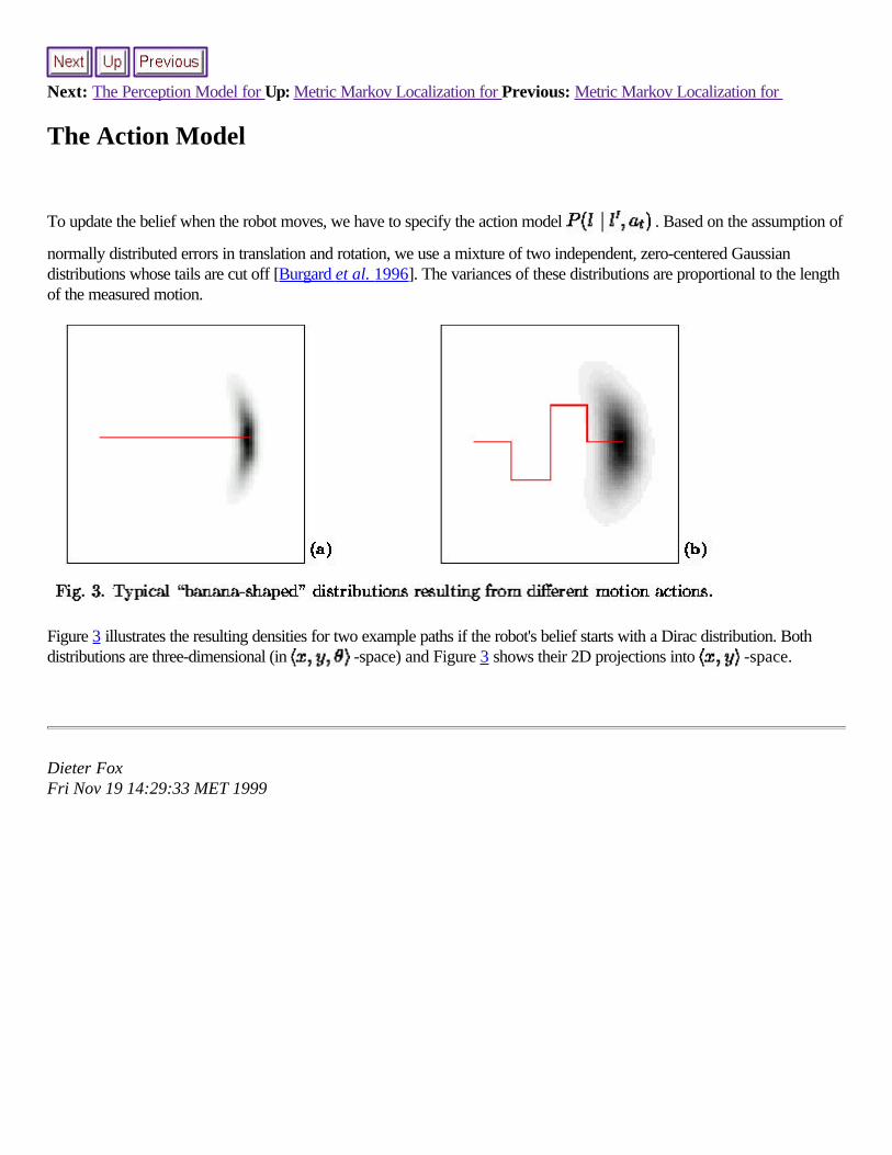
To update the belief when the robot moves, we have to specify the action model . Based on the assumption of

normally distributed errors in translation and rotation, we use a mixture of two independent, zero-centered Gaussiandistributions whose tails are cut off [Burgard et al. 1996]. The variances of these distributions are proportional to the lengthof the measured motion.

Figure 3 illustrates the resulting densities for two example paths if the robot's belief starts with a Dirac distribution. Bothdistributions are three-dimensional (in -space) and Figure 3 shows their 2D projections into -space.


Next: Filtering Techniques for Dynamic Up: Metric Markov Localization for Previous: The Action Model

The Perception Model for Proximity Sensors

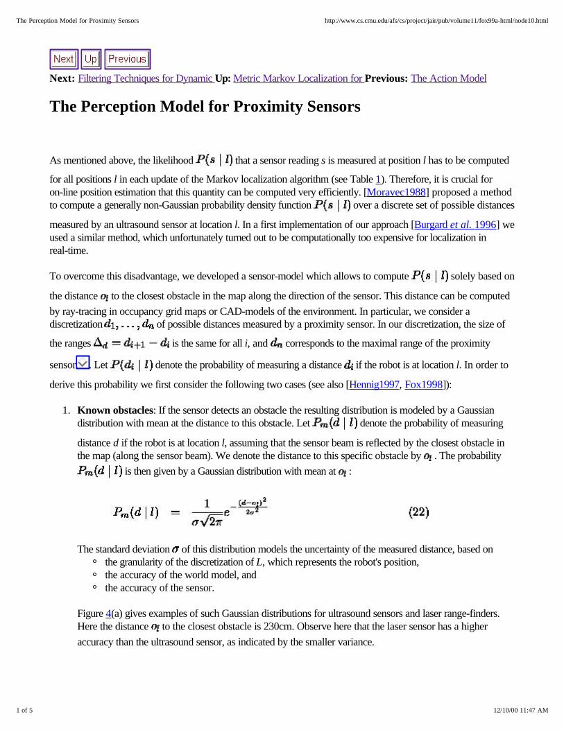
As mentioned above, the likelihood that a sensor reading s is measured at position l has to be computed

for all positions l in each update of the Markov localization algorithm (see Table 1). Therefore, it is crucial foron-line position estimation that this quantity can be computed very efficiently. [Moravec1988] proposed a methodto compute a generally non-Gaussian probability density function over a discrete set of possible distances

measured by an ultrasound sensor at location l. In a first implementation of our approach [Burgard et al. 1996] weused a similar method, which unfortunately turned out to be computationally too expensive for localization inreal-time.

To overcome this disadvantage, we developed a sensor-model which allows to compute solely based on

the distance to the closest obstacle in the map along the direction of the sensor. This distance can be computedby ray-tracing in occupancy grid maps or CAD-models of the environment. In particular, we consider adiscretization of possible distances measured by a proximity sensor. In our discretization, the size of

the ranges is the same for all i, and corresponds to the maximal range of the proximity

sensor . Let denote the probability of measuring a distance if the robot is at location l. In order to

derive this probability we first consider the following two cases (see also [Hennig1997, Fox1998]):

1. Known obstacles: If the sensor detects an obstacle the resulting distribution is modeled by a Gaussiandistribution with mean at the distance to this obstacle. Let denote the probability of measuring

distance d if the robot is at location l, assuming that the sensor beam is reflected by the closest obstacle inthe map (along the sensor beam). We denote the distance to this specific obstacle by . The probability

is then given by a Gaussian distribution with mean at :

The standard deviation of this distribution models the uncertainty of the measured distance, based on the granularity of the discretization of L, which represents the robot's position,the accuracy of the world model, andthe accuracy of the sensor.

Figure 4(a) gives examples of such Gaussian distributions for ultrasound sensors and laser range-finders.Here the distance to the closest obstacle is 230cm. Observe here that the laser sensor has a higheraccuracy than the ultrasound sensor, as indicated by the smaller variance.

1 of 5 12/10/00 11:47 AM

The Perception Model for Proximity Sensors http://www.cs.cmu.edu/afs/cs/project/jair/pub/volume11/fox99a-html/node10.html

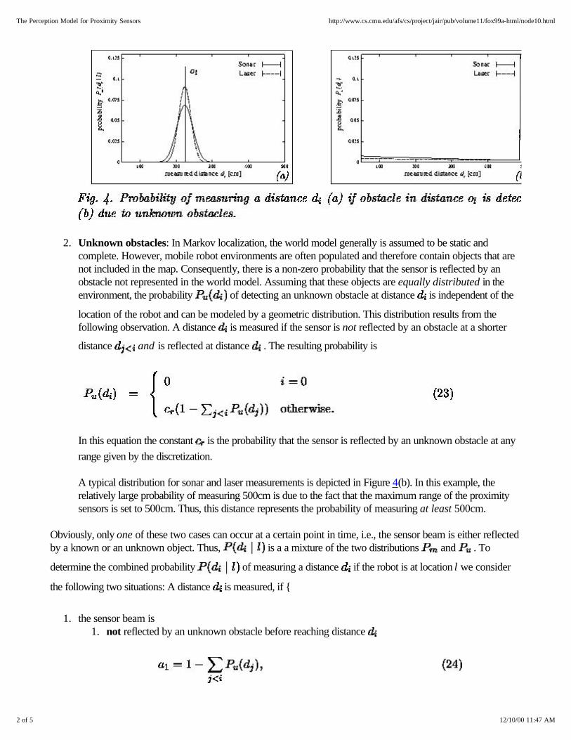
2. Unknown obstacles: In Markov localization, the world model generally is assumed to be static andcomplete. However, mobile robot environments are often populated and therefore contain objects that arenot included in the map. Consequently, there is a non-zero probability that the sensor is reflected by anobstacle not represented in the world model. Assuming that these objects are equally distributed in theenvironment, the probability of detecting an unknown obstacle at distance is independent of the

location of the robot and can be modeled by a geometric distribution. This distribution results from thefollowing observation. A distance is measured if the sensor is not reflected by an obstacle at a shorter

distance and is reflected at distance . The resulting probability is

In this equation the constant is the probability that the sensor is reflected by an unknown obstacle at anyrange given by the discretization.

A typical distribution for sonar and laser measurements is depicted in Figure 4(b). In this example, therelatively large probability of measuring 500cm is due to the fact that the maximum range of the proximitysensors is set to 500cm. Thus, this distance represents the probability of measuring at least 500cm.

Obviously, only one of these two cases can occur at a certain point in time, i.e., the sensor beam is either reflectedby a known or an unknown object. Thus, is a a mixture of the two distributions and . To

determine the combined probability of measuring a distance if the robot is at location l we consider

the following two situations: A distance is measured, if {

1. the sensor beam is 1. not reflected by an unknown obstacle before reaching distance

2 of 5 12/10/00 11:47 AM


2. and reflected by the known obstacle at distance

2. OR the beam is 1. reflected neither by an unknown obstacle nor by the known obstacle before reaching distance

2. and reflected by an unknown obstacle at distance

The parameter in Equation (25) denotes the probability that the sensor detects the closest obstacle in the map.These considerations for the combined probability are summarized in Equation (28). By double negation andinsertion of the Equations (24) to (27), we finally get Equation (31).

To obtain the probability of measuring , the maximal range of the sensor, we exploit the following equivalence:

The probability of measuring a distance larger than or equal to the maximal sensor range is equivalent to theprobability of not measuring a distance shorter than . In our incremental scheme, this probability can easily be

determined:

To summarize, the probability of sensor measurements is computed incrementally for the different distances startingat distance cm. For each distance we consider the probability that the sensor beam reaches the

corresponding distance and is reflected either by the closest obstacle in the map (along the sensor beam), or by anunknown obstacle.

3 of 5 12/10/00 11:47 AM


In order to adjust the parameters , and of our perception model we collected eleven million data pairsconsisting of the expected distance and the measured distance during the typical operation of the robot.

From these data we were able to estimate the probability of measuring a certain distance if the distance to the

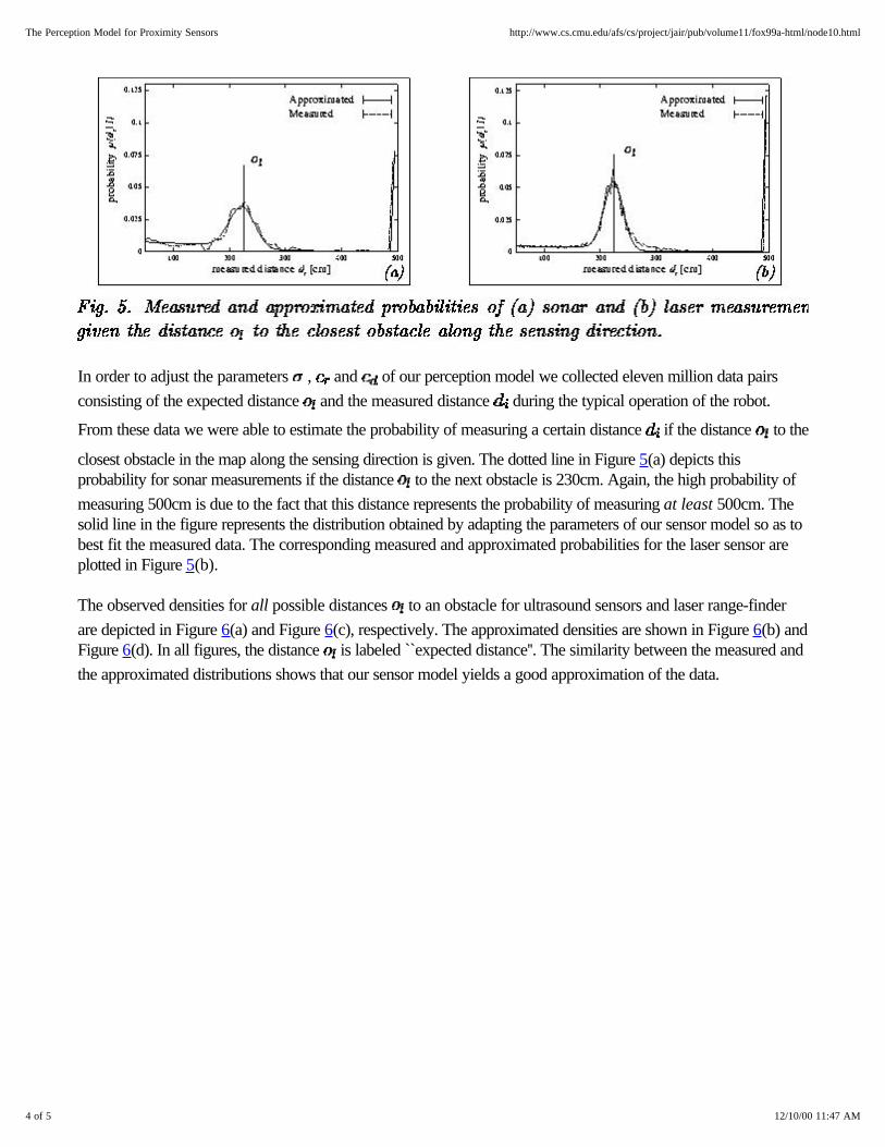
closest obstacle in the map along the sensing direction is given. The dotted line in Figure 5(a) depicts thisprobability for sonar measurements if the distance to the next obstacle is 230cm. Again, the high probability ofmeasuring 500cm is due to the fact that this distance represents the probability of measuring at least 500cm. Thesolid line in the figure represents the distribution obtained by adapting the parameters of our sensor model so as tobest fit the measured data. The corresponding measured and approximated probabilities for the laser sensor areplotted in Figure 5(b).

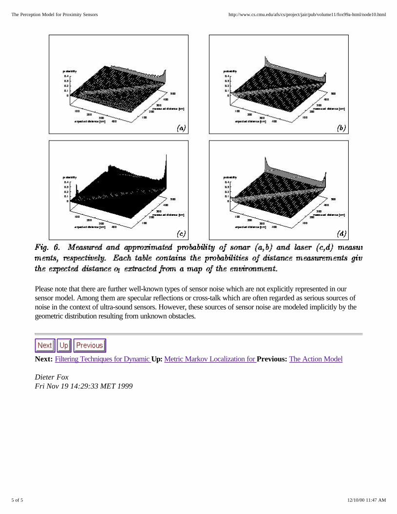
The observed densities for all possible distances to an obstacle for ultrasound sensors and laser range-finderare depicted in Figure 6(a) and Figure 6(c), respectively. The approximated densities are shown in Figure 6(b) andFigure 6(d). In all figures, the distance is labeled `èxpected distance''. The similarity between the measured andthe approximated distributions shows that our sensor model yields a good approximation of the data.

4 of 5 12/10/00 11:47 AM


Please note that there are further well-known types of sensor noise which are not explicitly represented in oursensor model. Among them are specular reflections or cross-talk which are often regarded as serious sources ofnoise in the context of ultra-sound sensors. However, these sources of sensor noise are modeled implicitly by thegeometric distribution resulting from unknown obstacles.

Next: Filtering Techniques for Dynamic Up: Metric Markov Localization for Previous: The Action Model


5 of 5 12/10/00 11:47 AM


Next: The Entropy Filter Up: Metric Markov Localization for Previous: The Perception Model for

Filtering Techniques for Dynamic Environments

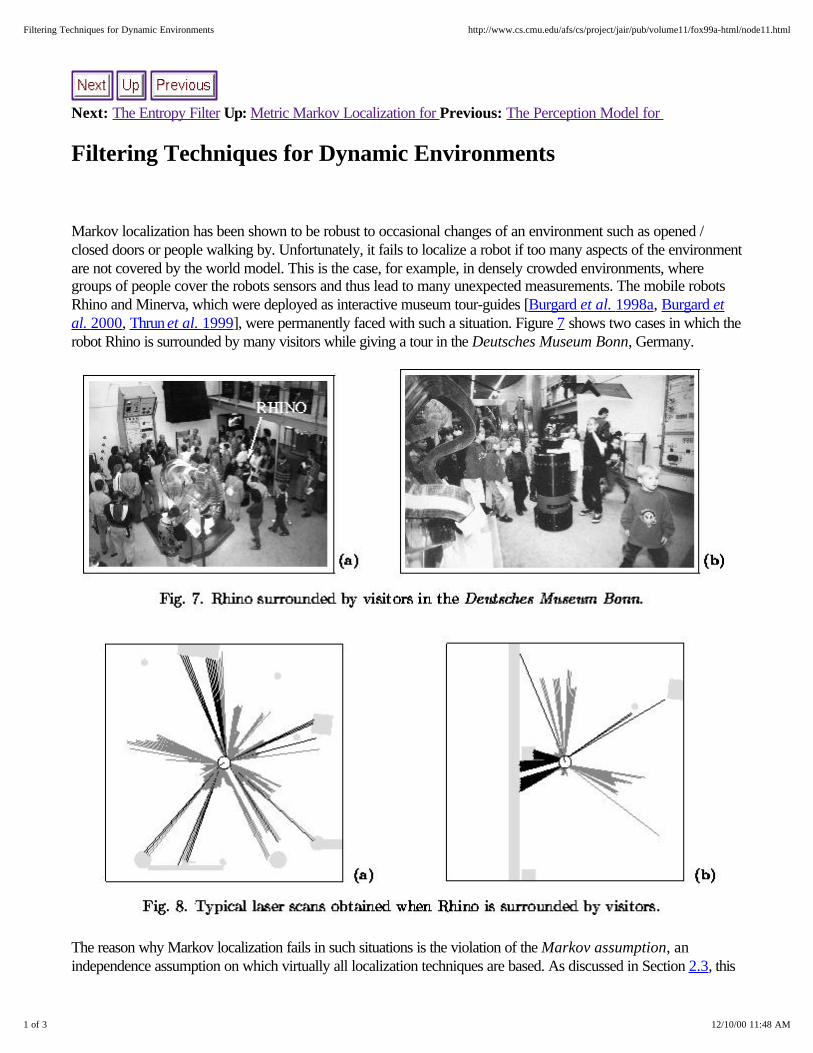
Markov localization has been shown to be robust to occasional changes of an environment such as opened /closed doors or people walking by. Unfortunately, it fails to localize a robot if too many aspects of the environmentare not covered by the world model. This is the case, for example, in densely crowded environments, wheregroups of people cover the robots sensors and thus lead to many unexpected measurements. The mobile robotsRhino and Minerva, which were deployed as interactive museum tour-guides [Burgard et al. 1998a, Burgard etal. 2000, Thrun et al. 1999], were permanently faced with such a situation. Figure 7 shows two cases in which therobot Rhino is surrounded by many visitors while giving a tour in the Deutsches Museum Bonn, Germany.

The reason why Markov localization fails in such situations is the violation of the Markov assumption, anindependence assumption on which virtually all localization techniques are based. As discussed in Section 2.3, this

1 of 3 12/10/00 11:48 AM

Filtering Techniques for Dynamic Environments http://www.cs.cmu.edu/afs/cs/project/jair/pub/volume11/fox99a-html/node11.html

assumption states that the sensor measurements observed at time t are independent of all other measurements,given that the current state of the world is known. In the case of localization in densely populated environments,

this independence assumption is clearly violated when using a static model of the world.

To illustrate this point, Figure 8 depicts two typical laser scans obtained during the museum projects (maximalrange measurements are omitted). The figure also shows the obstacles contained in the map. Obviously, thereadings are, to a large extent, corrupted, since people in the museum are not represented in the static worldmodel. The different shading of the beams indicates the two classes they belong to: the black lines correspond tothe static obstacles in the map and are independent of each other if the position of the robot is known. Thegrey-shaded lines are beams reflected by visitors in the Museum. These sensor beams cannot be predicted by theworld model and therefore are not independent of each other. Since the vicinity of people usually increases therobot's belief of being close to modeled obstacles, the robot quickly loses track of its position when incorporatingall sensor measurements. To reestablish the independence of sensor measurements we could include the positionof the robot and the position of people into the state variable L. Unfortunately, this is infeasible since thecomputational complexity of state estimation increases exponentially in the number of dependent state variables tobe estimated.

A closely related solution to this problem could be to adapt the map according to the changes of the environment.Techniques for concurrent map-building and localization such as [Lu & Milios1997, Gutmann & Schlegel1996,Shatkey & Kaelbling1997, Thrun et al. 1998b], however, also assume that the environment is almost static andtherefore are unable to deal with such environments. Another approach would be to adapt the perception model tocorrectly reflect such situations. Note that our perceptual model already assigns a certain probability to eventswhere the sensor beam is reflected by an unknown obstacle. Unfortunately, such approaches are only capable tomodel such noise on average. While such approaches turn out to work reliably with occasional sensor blockage,they are not sufficient in situations where more than fifty percent of the sensor measurements are corrupted. Ourlocalization system therefore includes filters which are designed to detect whether a certain sensor reading iscorrupted or not. Compared to a modification of the static sensor model described above, these filters have theadvantage that they do not average over all possible situations and that their decision is based on the current beliefof the robot.

The filters are designed to select those readings of a complete scan which do not come from objects contained inthe map. In this section we introduce two different kinds of filters. The first one is called entropy filter. Since itfilters a reading based solely on its effect on the belief Bel(L), it can be applied to arbitrary sensors. The secondfilter is the distance filter which selects the readings according to how much shorter they are than the expectedvalue. It therefore is especially designed for proximity sensors.


Next: The Entropy Filter Up: Metric Markov Localization for Previous: The Perception Model for

Dieter Fox

2 of 3 12/10/00 11:48 AM

Filtering Techniques for Dynamic Environments http://www.cs.cmu.edu/afs/cs/project/jair/pub/volume11/fox99a-html/node11.html

Next: The Distance Filter Up: Filtering Techniques for Dynamic Previous: Filtering Techniques for Dynamic

The Entropy Filter

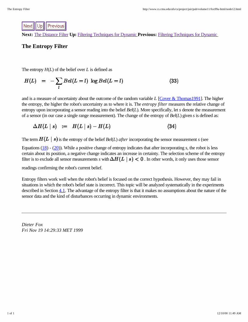
The entropy H(L) of the belief over L is defined as

and is a measure of uncertainty about the outcome of the random variable L [Cover & Thomas1991]. The higherthe entropy, the higher the robot's uncertainty as to where it is. The entropy filter measures the relative change ofentropy upon incorporating a sensor reading into the belief Bel(L). More specifically, let s denote the measurementof a sensor (in our case a single range measurement). The change of the entropy of Bel(L) given s is defined as:

The term is the entropy of the belief Bel(L) after incorporating the sensor measurement s (see

Equations (18) - (20)). While a positive change of entropy indicates that after incorporating s, the robot is lesscertain about its position, a negative change indicates an increase in certainty. The selection scheme of the entropyfilter is to exclude all sensor measurements s with . In other words, it only uses those sensor

readings confirming the robot's current belief.

Entropy filters work well when the robot's belief is focused on the correct hypothesis. However, they may fail insituations in which the robot's belief state is incorrect. This topic will be analyzed systematically in the experimentsdescribed in Section 4.1. The advantage of the entropy filter is that it makes no assumptions about the nature of thesensor data and the kind of disturbances occurring in dynamic environments.


1 of 1 12/10/00 11:49 AM

The Entropy Filter http://www.cs.cmu.edu/afs/cs/project/jair/pub/volume11/fox99a-html/node12.html

Next: Grid-based Representation of the Up: Filtering Techniques for Dynamic Previous: The Entropy Filter

The Distance Filter

The distance filter has specifically been designed for proximity sensors such as laser range-finders. Distance filtersare based on a simple observation: In proximity sensing, unmodeled obstacles typically produce readings that areshorter than the distance expected from the map. In essence, the distance filter selects sensor readings based ontheir distance relative to the distance to the closest obstacle in the map.

To be more specific, this filter removes those sensor measurements s which with probability higher than (this

threshold is set to 0.99 in all experiments) are shorter than expected, and which therefore are caused by anunmodeled object (e.g. a person).

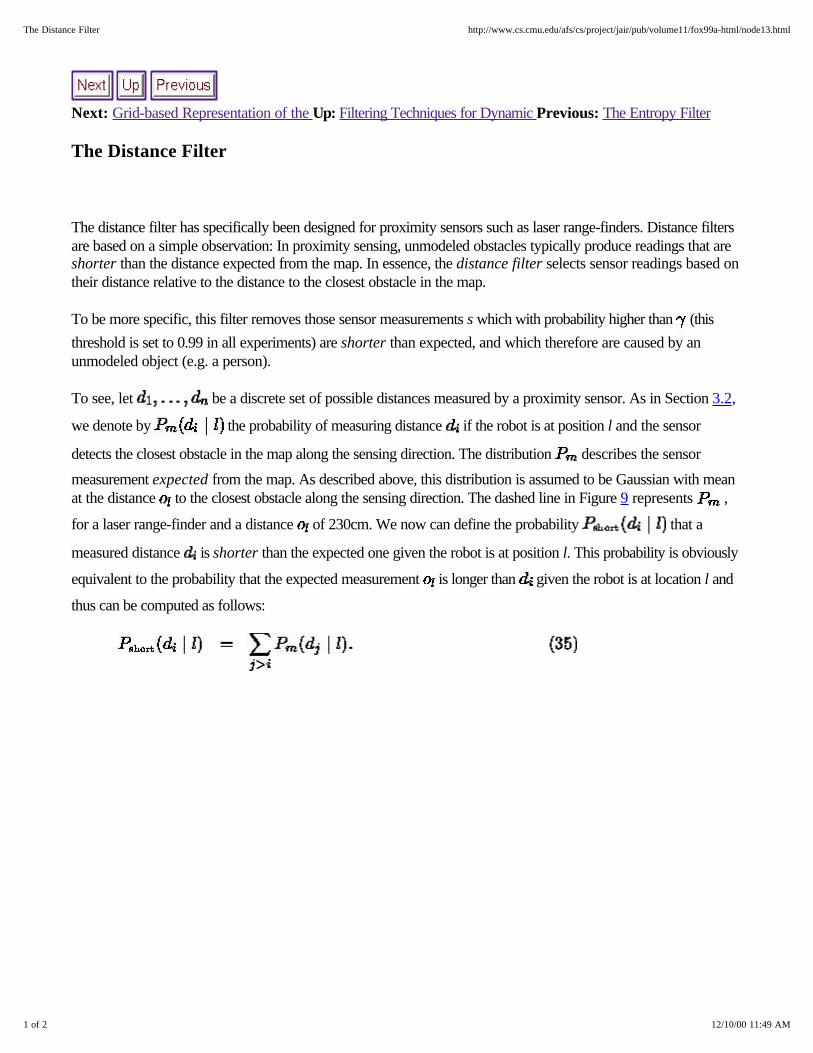
To see, let be a discrete set of possible distances measured by a proximity sensor. As in Section 3.2,

we denote by the probability of measuring distance if the robot is at position l and the sensor

detects the closest obstacle in the map along the sensing direction. The distribution describes the sensor

measurement expected from the map. As described above, this distribution is assumed to be Gaussian with meanat the distance to the closest obstacle along the sensing direction. The dashed line in Figure 9 represents ,

for a laser range-finder and a distance of 230cm. We now can define the probability that a

measured distance is shorter than the expected one given the robot is at position l. This probability is obviously

equivalent to the probability that the expected measurement is longer than given the robot is at location l and

thus can be computed as follows:

1 of 2 12/10/00 11:49 AM

The Distance Filter http://www.cs.cmu.edu/afs/cs/project/jair/pub/volume11/fox99a-html/node13.html

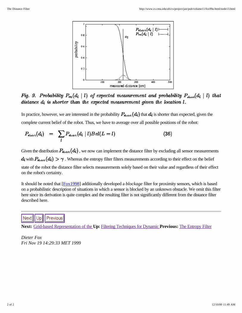
In practice, however, we are interested in the probability that is shorter than expected, given the

complete current belief of the robot. Thus, we have to average over all possible positions of the robot:

Given the distribution , we now can implement the distance filter by excluding all sensor measurements

with . Whereas the entropy filter filters measurements according to their effect on the belief

state of the robot the distance filter selects measurements solely based on their value and regardless of their effecton the robot's certainty.

It should be noted that [Fox1998] additionally developed a blockage filter for proximity sensors, which is basedon a probabilistic description of situations in which a sensor is blocked by an unknown obstacle. We omit this filterhere since its derivation is quite complex and the resulting filter is not significantly different from the distance filterdescribed here.

Next: Grid-based Representation of the Up: Filtering Techniques for Dynamic Previous: The Entropy Filter


2 of 2 12/10/00 11:49 AM

The Distance Filter http://www.cs.cmu.edu/afs/cs/project/jair/pub/volume11/fox99a-html/node13.html

Next: Pre-Computation of the Sensor Up: Metric Markov Localization for Previous: The Distance Filter

Grid-based Representation of the State Space

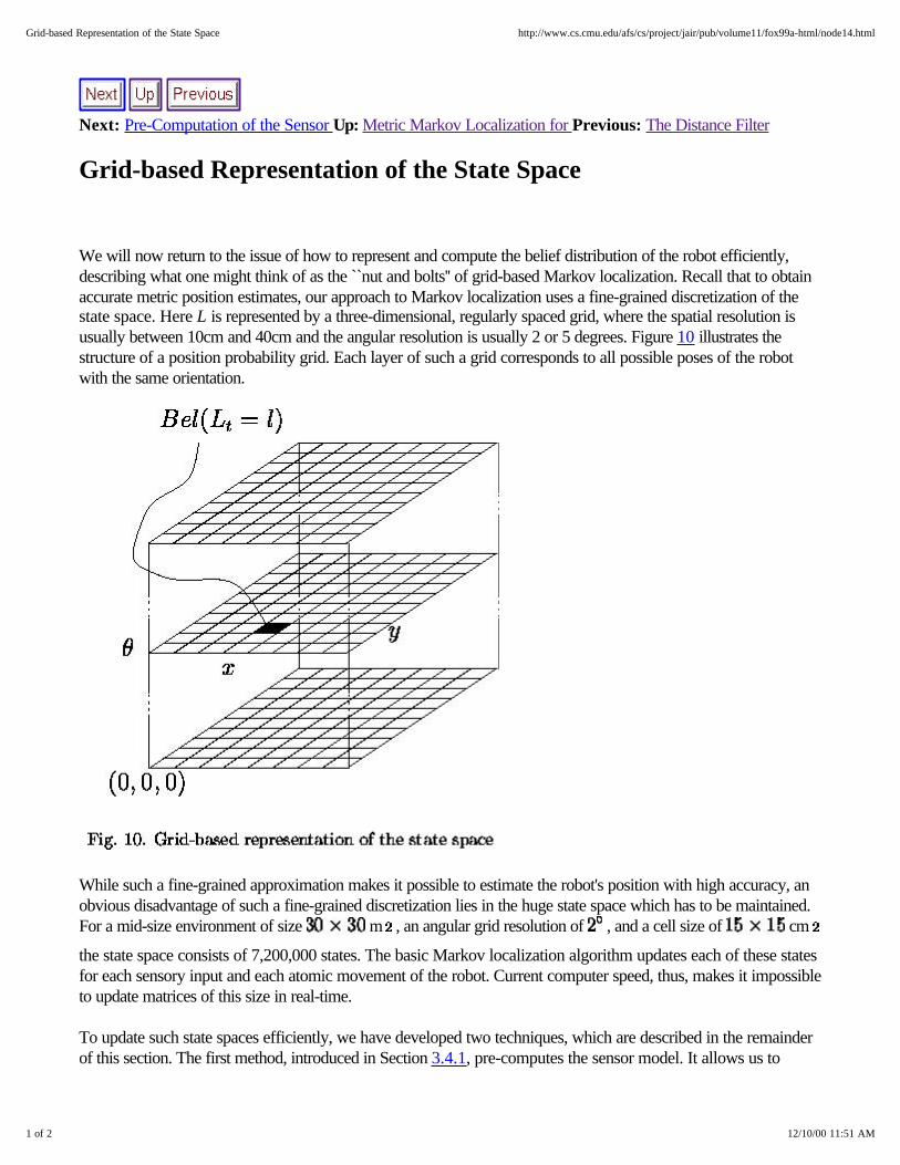
We will now return to the issue of how to represent and compute the belief distribution of the robot efficiently,describing what one might think of as the ``nut and bolts'' of grid-based Markov localization. Recall that to obtainaccurate metric position estimates, our approach to Markov localization uses a fine-grained discretization of thestate space. Here L is represented by a three-dimensional, regularly spaced grid, where the spatial resolution isusually between 10cm and 40cm and the angular resolution is usually 2 or 5 degrees. Figure 10 illustrates thestructure of a position probability grid. Each layer of such a grid corresponds to all possible poses of the robotwith the same orientation.

While such a fine-grained approximation makes it possible to estimate the robot's position with high accuracy, anobvious disadvantage of such a fine-grained discretization lies in the huge state space which has to be maintained.For a mid-size environment of size m , an angular grid resolution of , and a cell size of cm

the state space consists of 7,200,000 states. The basic Markov localization algorithm updates each of these statesfor each sensory input and each atomic movement of the robot. Current computer speed, thus, makes it impossibleto update matrices of this size in real-time.

To update such state spaces efficiently, we have developed two techniques, which are described in the remainderof this section. The first method, introduced in Section 3.4.1, pre-computes the sensor model. It allows us to

1 of 2 12/10/00 11:51 AM

Grid-based Representation of the State Space http://www.cs.cmu.edu/afs/cs/project/jair/pub/volume11/fox99a-html/node14.html

determine the likelihood of sensor measurements by two look-up operations--instead of expensive ray

tracing operations. The second optimization, described in Section 3.4.2, is a selective update strategy. Thisstrategy focuses the computation, by only updating the relevant part of the state space. Based on these twotechniques, grid-based Markov localization can be applied on-line to estimate the position of a mobile robot duringits operation, using a low-cost PC.

Pre-Computation of the Sensor Model Selective Update

Next: Pre-Computation of the Sensor Up: Metric Markov Localization for Previous: The Distance Filter


2 of 2 12/10/00 11:51 AM

Grid-based Representation of the State Space http://www.cs.cmu.edu/afs/cs/project/jair/pub/volume11/fox99a-html/node14.html

Next: Selective Update Up: Grid-based Representation of the Previous: Grid-based Representation of the

Pre-Computation of the Sensor Model

As described in Section 3.2, the perception model for proximity sensors only depends on the distance

to the closest obstacle in the map along the sensor beam. Based on the assumption that the map of the environmentis static, our approach pre-computes and stores these distances for each possible robot location l in theenvironment. Following our sensor model, we use a discretization of the possible distances . This

discretization is exactly the same for the expected and the measured distances. We then store for each location lonly the index of the expected distance in a three-dimensional table. Please note that this table only needs onebyte per value if 256 different values for the discretization of are used. The probability of measuring

a distance if the closest obstacle is at distance (see Figure 6) can also be pre-computed and stored in a

two-dimensional lookup-table.

As a result, the probability of measuring s given a location l can quickly be computed by two nested

lookups. The first look-up retrieves the distance to the closest obstacle in the sensing direction given the robot isat location l. The second lookup is then used to get the probability . The efficient computation based on

table look-ups enabled our implementation to quickly incorporate even laser-range scans that consist of up to 180values in the overall belief state of the robot. In our experiments, the use of the look-up tables led to aspeed-up-factor of 10, when compared to a computation of the distance to the closest obstacle at run-time.


1 of 1 12/10/00 11:51 AM

Pre-Computation of the Sensor Model http://www.cs.cmu.edu/afs/cs/project/jair/pub/volume11/fox99a-html/node15.html

Next: Experimental Results Up: Grid-based Representation of the Previous: Pre-Computation of the Sensor

Selective Update

The selective update scheme is based on the observation that during global localization, the certainty of theposition estimation permanently increases and the density quickly concentrates on the grid cells representing thetrue position of the robot. The probability of the other grid cells decreases during localization and the key idea ofour optimization is to exclude unlikely cells from being updated.

For this purpose, we introduce a threshold and update only those grid cells l with . To

allow for such a selective update while still maintaining a density over the entire state space, we approximate for cells with by the a priori probability of measuring . This quantity, which we

call , is determined by averaging over all possible locations of the robot:

Please note that is independent of the current belief state of the robot and can be determined beforehand.

The incremental update rule for a new sensor measurement is changed as follows (compare Equation (9)):

By multiplying into the normalization factor , we can rewrite this equation as

where .

The key advantage of the selective update scheme given in Equation (39) is that all cells with are updated with the same value . In order to obtain smooth transitions between global

localization and position tracking and to focus the computation on the important regions of the state space L, forexample, in the case of ambiguities we use a partitioning of the state space. Suppose the state space L ispartitioned into n segments or parts . A segment is called active at time t if it contains locations

1 of 3 12/10/00 12:02 PM

Selective Update http://www.cs.cmu.edu/afs/cs/project/jair/pub/volume11/fox99a-html/node16.html

with probability above the threshold ; otherwise we call such a part passive because the probabilities of all cellsare below the threshold. Obviously, we can keep track of the individual probabilities within a passive part byaccumulating the normalization factors into a value . Whenever a segment becomes passive, i.e. the

probabilities of all locations within no longer exceed , the normalizer is initialized to 1 and subsequently

updated as follows: . As soon as a part becomes active again, we can restore the

probabilities of the individual grid cells by multiplying the probabilities of each cell with the accumulated normalizer . By keeping track of the robot motion since a part became passive, it suffices to incorporate the

accumulated motion whenever the part becomes active again. In order to efficiently detect whether a passive parthas to be activated again, we store the maximal probability of all cells in the part at the time it becomes

passive. Whenever exceeds , the part is activated again because it contains at least one

position with probability above the threshold. In our current implementation we partition the state space L suchthat each part consists of all locations with equal orientation relative to the robot's start location.

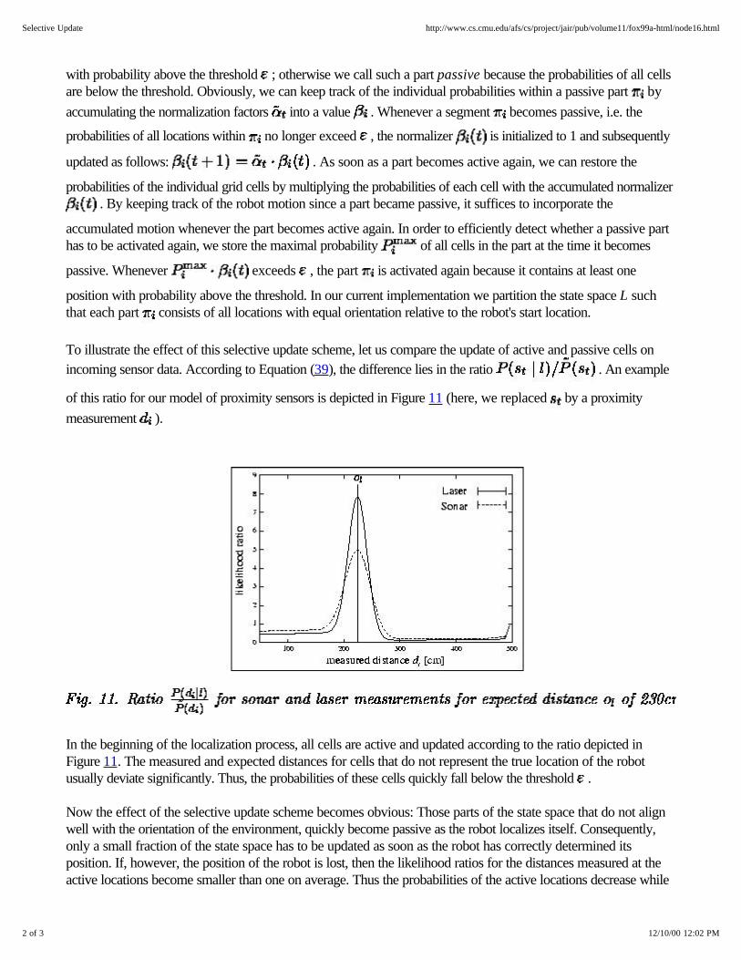
To illustrate the effect of this selective update scheme, let us compare the update of active and passive cells onincoming sensor data. According to Equation (39), the difference lies in the ratio . An example

of this ratio for our model of proximity sensors is depicted in Figure 11 (here, we replaced by a proximitymeasurement ).

In the beginning of the localization process, all cells are active and updated according to the ratio depicted inFigure 11. The measured and expected distances for cells that do not represent the true location of the robotusually deviate significantly. Thus, the probabilities of these cells quickly fall below the threshold .

Now the effect of the selective update scheme becomes obvious: Those parts of the state space that do not alignwell with the orientation of the environment, quickly become passive as the robot localizes itself. Consequently,only a small fraction of the state space has to be updated as soon as the robot has correctly determined itsposition. If, however, the position of the robot is lost, then the likelihood ratios for the distances measured at theactive locations become smaller than one on average. Thus the probabilities of the active locations decrease while

2 of 3 12/10/00 12:02 PM


the normalizers of the passive parts increase until these segments are activated again. Once the true position of

the robot is among the active locations, the robot is able to re-establish the correct belief.

In extensive experimental tests we did not observe evidence that the selective update scheme has a noticablynegative impact on the robot's behavior. In contrast, it turned out to be highly effective, since in practice only asmall fraction (generally less than 5%) of the state space has to be updated once the position of the robot hasbeen determined correctly, and the probabilities of the active locations generally sum up to at least 0.99. Thus, theselective update scheme automatically adapts the computation time required to update the belief to the certainty ofthe robot. This way, our system is able to efficiently track the position of a robot once its position has beendetermined. Additionally, Markov localization keeps the ability to detect localization failures and to relocalize therobot. The only disadvantage lies in the fixed representation of the grid which has the undesirable effect that thememory requirement in our current implementation stays constant even if only a minor part of the state space isupdated. In this context we would like to mention that recently promising techniques have been presented toovercome this disadvantage by applying alternative and dynamic representations of the state space [Burgard et al.1998b, Fox et al. 1999].

Next: Experimental Results Up: Grid-based Representation of the Previous: Pre-Computation of the Sensor


3 of 3 12/10/00 12:02 PM


Next: Long-term Experiments in Dynamic Up: Markov Localization for Mobile Previous: Selective Update

Experimental Results

Our metric Markov localization technique, including both sensor filters, has been implemented and evaluatedextensively in various environments. In this section we present some of the experiments carried out with the mobilerobots Rhino and Minerva (see Figure 1). Rhino has a ring of 24 ultrasound sensors each with an opening angle of15 degrees. Both, Rhino and Minerva are equipped with two laser range-finders covering a 360 degrees field ofview.

The first set of experiments demonstrates the robustness of Markov localization in two real-world scenarios. Inparticular, it systematically evaluates the effect of the filtering techniques on the localization performance in highlydynamic environments. An additional experiment illustrates a further advantage of the filtering technique, whichenables a mobile robot to reliably estimate its position even if only an outline of an office environment is given as amap.

In further experiments described in this section, we will illustrate the ability of our Markov localization technique toglobally localize a mobile robot in approximate world models such as occupancy grid maps, even when usinginaccurate sensors such as ultrasound sensors. Finally, we present experiments analyzing the accuracy andefficiency of grid-based Markov localization with respect to the size of the grid cells.

The experiments reported here demonstrate that Markov localization is able to globally estimate the position of amobile robot, and to reliably keep track of it even if only an approximate model of a possibly dynamicenvironment is given, if the robot has a weak odometry, and if noisy sensors such as ultrasound sensors are used.

Long-term Experiments in Dynamic Environments Datasets Tracking the Robot's Position Recovery from Extreme Localization Failures

Localization in Incomplete Maps Localization in Occupancy Grid Maps Using Sonar Precision and Performance


1 of 1 12/10/00 12:03 PM

Experimental Results http://www.cs.cmu.edu/afs/cs/project/jair/pub/volume11/fox99a-html/node17.html

Next: Datasets Up: Experimental Results Previous: Experimental Results

Long-term Experiments in Dynamic Environments

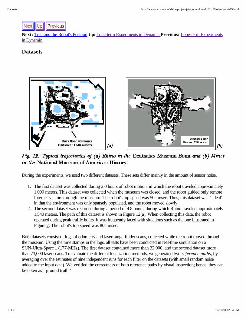
For our mobile robots Rhino and Minerva, which operated in the Deutsches Museum Bonn and theUS-Smithsonian's National Museum of American History, the robustness and reliability of our Markovlocalization system was of utmost importance. Accurate position estimation was a crucial component, as many ofthe obstacles were `ìnvisible'' to the robots' sensors (such as glass cages, metal bars, staircases, and the alike).Given the estimate of the robot's position [Fox et al. 1998b] integrated map information into the collisionavoidance system in order to prevent the robot from colliding with obstacles that could not be detected.Figure 12(a) shows a typical trajectory of the robot Rhino, recorded in the museum in Bonn, along with the mapused for localization. The reader may notice that only the obstacles shown in black were actually used forlocalization; the others were either invisible or could not be detected reliably. Rhino used the entropy filter toidentify sensor readings that were corrupted by the presence of people. Rhino's localization module was able to(1) globally localize the robot in the morning when the robot was switched on and (2) to reliably and accuratelykeep track of the robot's position. In the entire six-day deployment period, in which Rhino traveled over 18km,our approach led only to a single software-related collision, which involved an `ìnvisible'' obstacle and which wascaused by a localization error that was slightly larger than a 30cm safety margin.

Figure 12(b) shows a 2km long trajectory of the robot Minerva in the National Museum of American History.Minerva used the distance filter to identify readings reflected by unmodeled objects. This filter was developedafter Rhino's deployment in the museum in Bonn, based on an analysis of the localization failure reported aboveand in an attempt to prevent similar effects in future installations. Based on the distance filter, Minerva was able tooperate reliably over a period of 13 days. During that time Minerva traveled a total of 44km with a maximumspeed of 1.63m/sec.

Unfortunately, the evidence from the museum projects is anecdotal. Based on sensor data collected during Rhino'sdeployment in the museum in Bonn, we also investigated the effect of our filter techniques more systematically, andunder even more extreme conditions. In particular, we were interested in the localization results

1. when the environment is densely populated (more than 50% of the sensor reading are corrupted), and2. when the robot suffers extreme dead-reckoning errors (e.g. induced by a person carrying the robot

somewhere else). Since such cases are rare, we manually inflicted such errors into the original data toanalyze their effect.

Datasets Tracking the Robot's Position Recovery from Extreme Localization Failures

1 of 2 12/10/00 12:04 PM

Long-term Experiments in Dynamic Environments http://www.cs.cmu.edu/afs/cs/project/jair/pub/volume11/fox99a-html/node18.html

Next: Datasets Up: Experimental Results Previous: Experimental Results


2 of 2 12/10/00 12:04 PM

Long-term Experiments in Dynamic Environments http://www.cs.cmu.edu/afs/cs/project/jair/pub/volume11/fox99a-html/node18.html

Next: Tracking the Robot's Position Up: Long-term Experiments in Dynamic Previous: Long-term Experimentsin Dynamic

Datasets

During the experiments, we used two different datasets. These sets differ mainly in the amount of sensor noise.

1. The first dataset was collected during 2.0 hours of robot motion, in which the robot traveled approximately1,000 meters. This dataset was collected when the museum was closed, and the robot guided only remoteInternet-visitors through the museum. The robot's top speed was 50cm/sec. Thus, this dataset was `ìdeal''in that the environment was only sparsely populated, and the robot moved slowly.

2. The second dataset was recorded during a period of 4.8 hours, during which Rhino traveled approximately1,540 meters. The path of this dataset is shown in Figure 12(a). When collecting this data, the robotoperated during peak traffic hours. It was frequently faced with situations such as the one illustrated inFigure 7. The robot's top speed was 80cm/sec.

Both datasets consist of logs of odometry and laser range-finder scans, collected while the robot moved throughthe museum. Using the time stamps in the logs, all tests have been conducted in real-time simulation on aSUN-Ultra-Sparc 1 (177-MHz). The first dataset contained more than 32,000, and the second dataset morethan 73,000 laser scans. To evaluate the different localization methods, we generated two reference paths, byaveraging over the estimates of nine independent runs for each filter on the datasets (with small random noiseadded to the input data). We verified the correctness of both reference paths by visual inspection; hence, they canbe taken as ``ground truth.''

1 of 2 12/10/00 12:04 PM

Datasets http://www.cs.cmu.edu/afs/cs/project/jair/pub/volume11/fox99a-html/node19.html

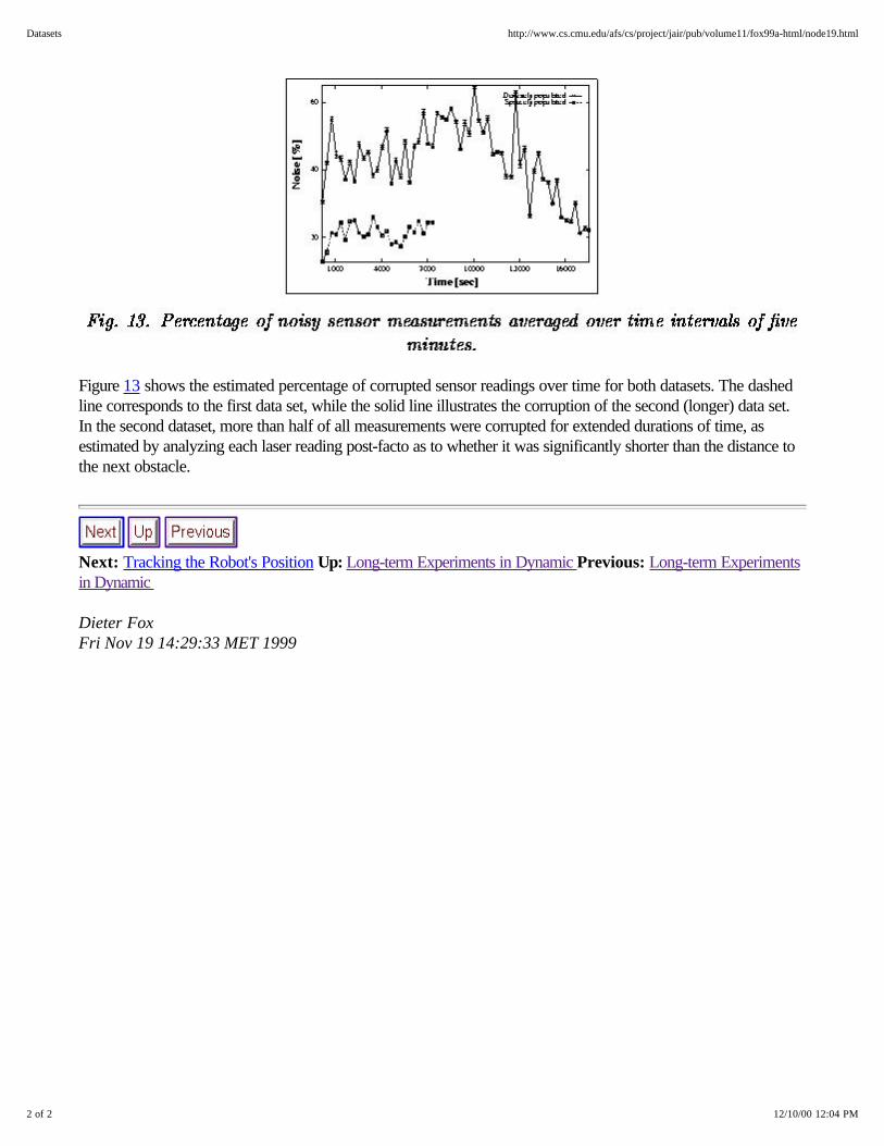
Figure 13 shows the estimated percentage of corrupted sensor readings over time for both datasets. The dashedline corresponds to the first data set, while the solid line illustrates the corruption of the second (longer) data set.In the second dataset, more than half of all measurements were corrupted for extended durations of time, asestimated by analyzing each laser reading post-facto as to whether it was significantly shorter than the distance tothe next obstacle.

Next: Tracking the Robot's Position Up: Long-term Experiments in Dynamic Previous: Long-term Experimentsin Dynamic


2 of 2 12/10/00 12:04 PM

Datasets http://www.cs.cmu.edu/afs/cs/project/jair/pub/volume11/fox99a-html/node19.html

Next: Recovery from Extreme Localization Up: Long-term Experiments in Dynamic Previous: Datasets

Tracking the Robot's Position

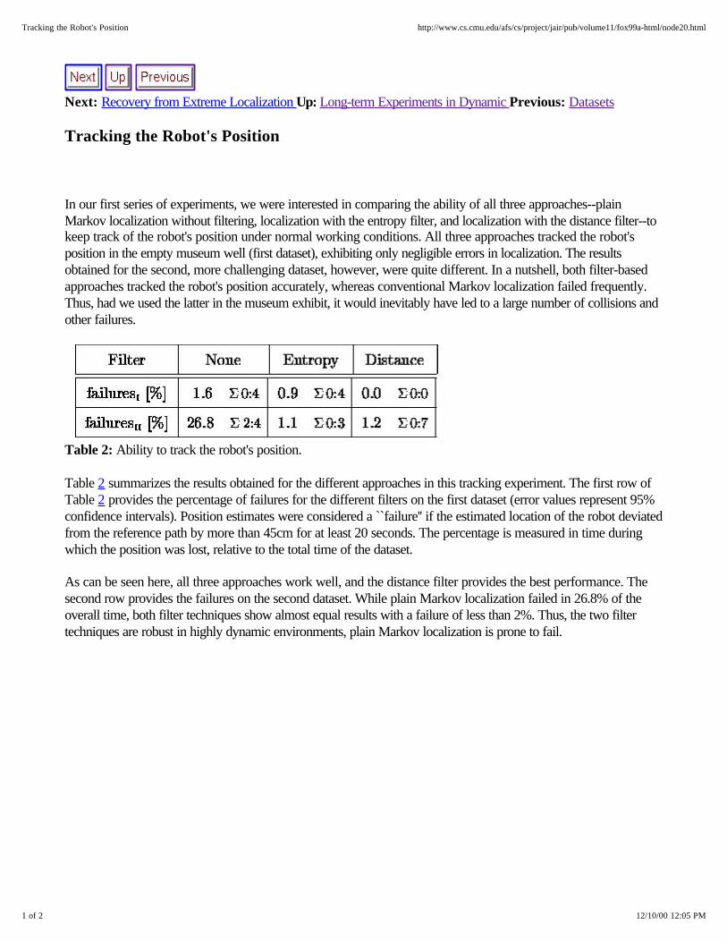
In our first series of experiments, we were interested in comparing the ability of all three approaches--plainMarkov localization without filtering, localization with the entropy filter, and localization with the distance filter--tokeep track of the robot's position under normal working conditions. All three approaches tracked the robot'sposition in the empty museum well (first dataset), exhibiting only negligible errors in localization. The resultsobtained for the second, more challenging dataset, however, were quite different. In a nutshell, both filter-basedapproaches tracked the robot's position accurately, whereas conventional Markov localization failed frequently.Thus, had we used the latter in the museum exhibit, it would inevitably have led to a large number of collisions andother failures.

Table 2: Ability to track the robot's position.

Table 2 summarizes the results obtained for the different approaches in this tracking experiment. The first row ofTable 2 provides the percentage of failures for the different filters on the first dataset (error values represent 95%confidence intervals). Position estimates were considered a ``failure'' if the estimated location of the robot deviatedfrom the reference path by more than 45cm for at least 20 seconds. The percentage is measured in time duringwhich the position was lost, relative to the total time of the dataset.

As can be seen here, all three approaches work well, and the distance filter provides the best performance. Thesecond row provides the failures on the second dataset. While plain Markov localization failed in 26.8% of theoverall time, both filter techniques show almost equal results with a failure of less than 2%. Thus, the two filtertechniques are robust in highly dynamic environments, plain Markov localization is prone to fail.

1 of 2 12/10/00 12:05 PM

Tracking the Robot's Position http://www.cs.cmu.edu/afs/cs/project/jair/pub/volume11/fox99a-html/node20.html

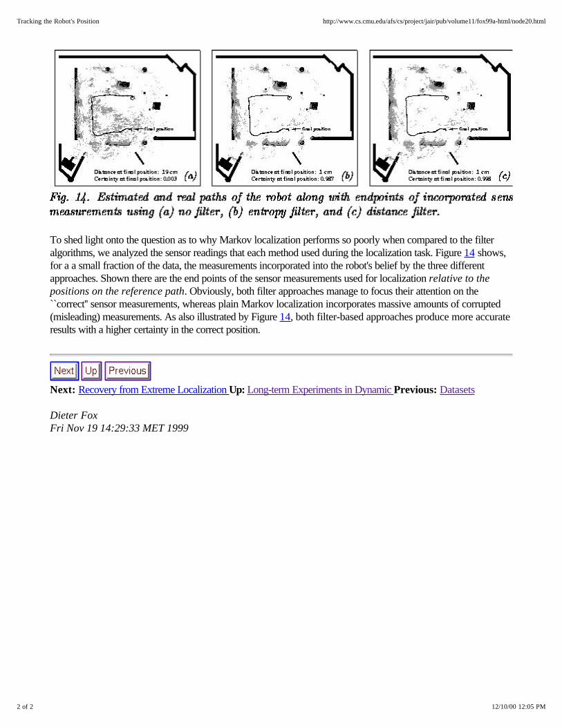
To shed light onto the question as to why Markov localization performs so poorly when compared to the filteralgorithms, we analyzed the sensor readings that each method used during the localization task. Figure 14 shows,for a a small fraction of the data, the measurements incorporated into the robot's belief by the three differentapproaches. Shown there are the end points of the sensor measurements used for localization relative to thepositions on the reference path. Obviously, both filter approaches manage to focus their attention on the``correct'' sensor measurements, whereas plain Markov localization incorporates massive amounts of corrupted(misleading) measurements. As also illustrated by Figure 14, both filter-based approaches produce more accurateresults with a higher certainty in the correct position.

Next: Recovery from Extreme Localization Up: Long-term Experiments in Dynamic Previous: Datasets


2 of 2 12/10/00 12:05 PM

Tracking the Robot's Position http://www.cs.cmu.edu/afs/cs/project/jair/pub/volume11/fox99a-html/node20.html

Next: Localization in Incomplete Maps Up: Long-term Experiments in Dynamic Previous: Tracking the Robot'sPosition

Recovery from Extreme Localization Failures

We conjecture that a key advantage of the original Markov localization technique lies in its ability to recover fromextreme localization failures. Re-localization after a failure is often more difficult than global localization fromscratch, since the robot starts with a belief that is centered at a completely wrong position. Since the filteringtechniques use the current belief to select the readings that are incorporated, it is not clear that they still maintainthe ability to recover from global localization failures.

To analyze the behavior of the filters under such extreme conditions, we carried out a series of experiments duringwhich we manually introduced such failures into the data to test the robustness of these methods in the extreme.More specifically, we ``tele-ported'' the robot at random points in time to other locations. Technically, this wasdone by changing the robot's orientation by 180 degree and shifting it by 0 cm, without letting the

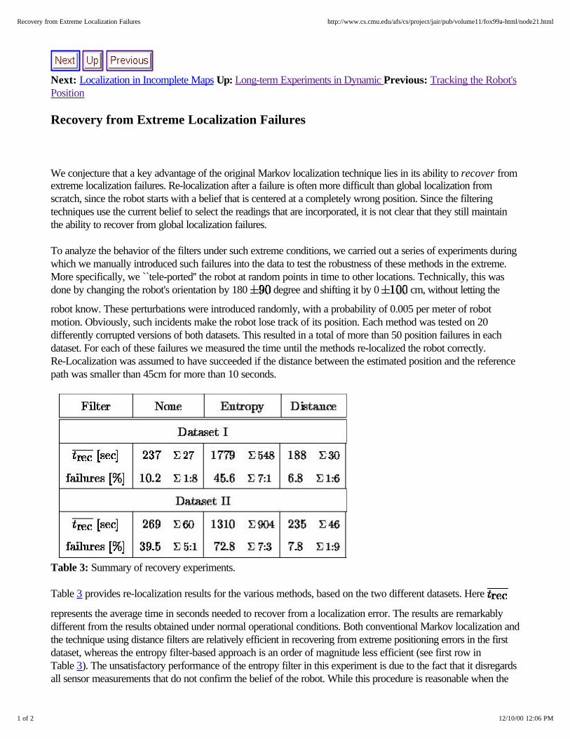
robot know. These perturbations were introduced randomly, with a probability of 0.005 per meter of robotmotion. Obviously, such incidents make the robot lose track of its position. Each method was tested on 20differently corrupted versions of both datasets. This resulted in a total of more than 50 position failures in eachdataset. For each of these failures we measured the time until the methods re-localized the robot correctly.Re-Localization was assumed to have succeeded if the distance between the estimated position and the referencepath was smaller than 45cm for more than 10 seconds.

Table 3: Summary of recovery experiments.

Table 3 provides re-localization results for the various methods, based on the two different datasets. Here

represents the average time in seconds needed to recover from a localization error. The results are remarkablydifferent from the results obtained under normal operational conditions. Both conventional Markov localization andthe technique using distance filters are relatively efficient in recovering from extreme positioning errors in the firstdataset, whereas the entropy filter-based approach is an order of magnitude less efficient (see first row inTable 3). The unsatisfactory performance of the entropy filter in this experiment is due to the fact that it disregardsall sensor measurements that do not confirm the belief of the robot. While this procedure is reasonable when the

1 of 2 12/10/00 12:06 PM

Recovery from Extreme Localization Failures http://www.cs.cmu.edu/afs/cs/project/jair/pub/volume11/fox99a-html/node21.html

belief is correct, it prevents the robot from detecting localization failures. The percentage of time when the positionof the robot was lost in the entire run is given in the second row of the table. Please note that this percentageincludes both, failures due to manually introduced perturbations and tracking failures. Again, the distance filter isslightly better than the approach without filter, while the entropy filter performs poorly. The average times to

recover from failures on the second dataset are similar to those in the first dataset. The bottom row in Table 3provides the percentage of failures for this more difficult dataset. Here the distance filter-based approach performssignificantly better than both other approaches, since it is able to quickly recover from localization failures and toreliably track the robot's position.

The results illustrate that despite the fact that sensor readings are processed selectively, the distance filter-basedtechnique recovers as efficiently from extreme localization errors as the conventional Markov approach.

Next: Localization in Incomplete Maps Up: Long-term Experiments in Dynamic Previous: Tracking the Robot'sPosition


2 of 2 12/10/00 12:06 PM

Recovery from Extreme Localization Failures http://www.cs.cmu.edu/afs/cs/project/jair/pub/volume11/fox99a-html/node21.html

Next: Localization in Occupancy Grid Up: Experimental Results Previous: Recovery from Extreme Localization

Localization in Incomplete Maps

A further advantage of the filtering techniques is that Markov localization does not require a detailed map of theenvironment. Instead, it suffices to provide only an outline which merely includes the aspects of the world whichare static.

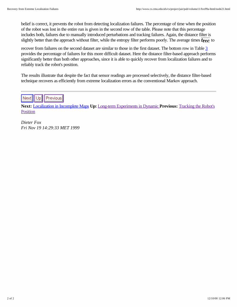
Figure 15(a) shows a ground plan of our department building, which contains only the walls of the universitybuilding. The complete map, including all movable objects such as tables and chairs, is shown in Figure 19. Thetwo Figures 15(b) and 15(c) illustrate how the distance filter typically behaves when tracking the robot's positionin such a sparse map of the environment. Filtered readings are shown in grey, and the incorporated sensorreadings are shown in black. Obviously, the filter focuses on the known aspects of the map and ignores all objects(such as desks, chairs, doors and tables) which are not contained in the outline. [Fox1998] describes moresystematic experiments supporting our belief that Markov localization in combination with the distance filter is ableto accurately localize mobile robots even when relying only on an outline of the environment.


1 of 1 12/10/00 12:18 PM

Localization in Incomplete Maps http://www.cs.cmu.edu/afs/cs/project/jair/pub/volume11/fox99a-html/node22.html

Next: Precision and Performance Up: Experimental Results Previous: Localization in Incomplete Maps

Localization in Occupancy Grid Maps Using Sonar

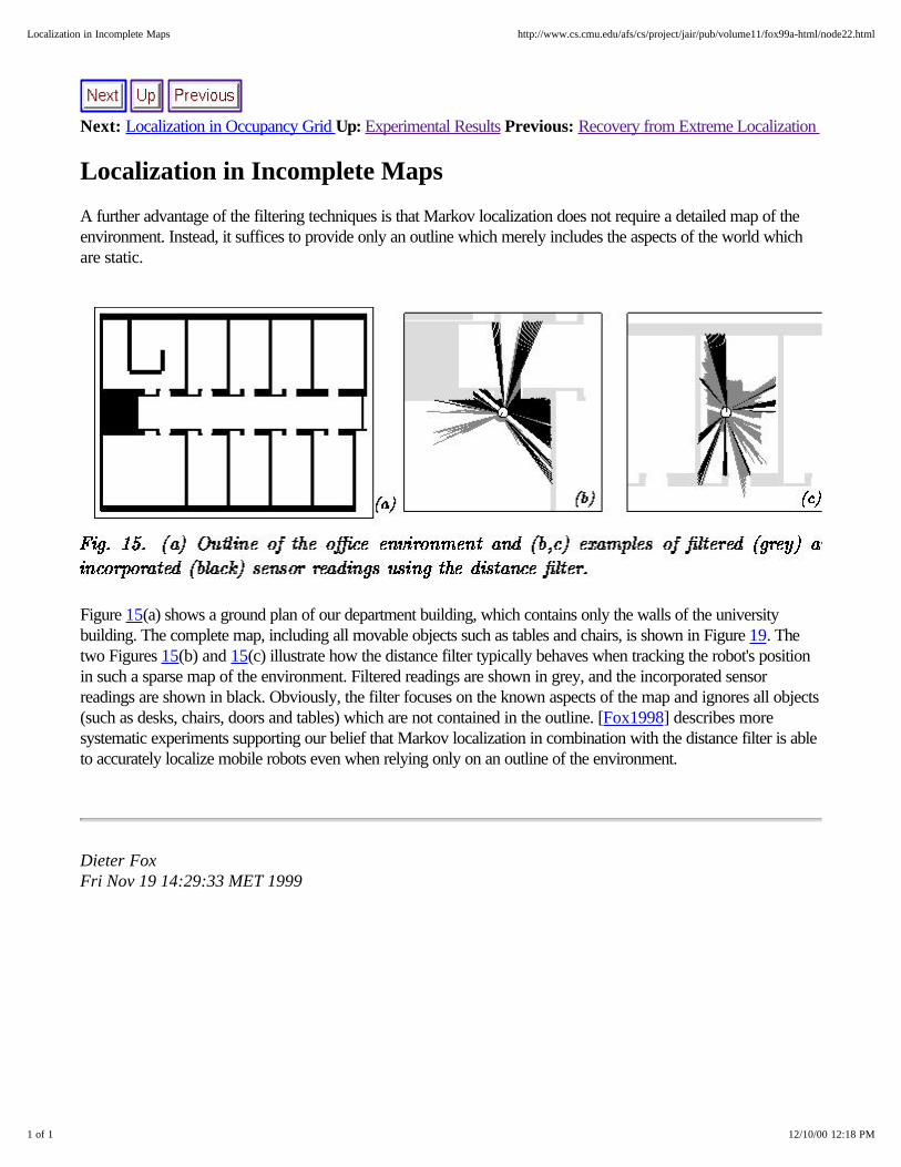
The next experiment described here is carried out based on data collected with the mobile robot Rhino during the1994 AAAI mobile robot competition [Simmons1995]. Figure 16(a) shows an occupancy grid map [Moravec &Elfes1985, Moravec1988] of the environment, constructed with the techniques described in [Thrun et al. 1998a,Thrun1998b]. The size of the map is , and the grid resolution is 15cm.

Figure 16(b) shows a trajectory of the robot along with measurements of the 24 ultrasound sensors obtained asthe robot moved through the competition arena. Here we use this sensor information to globally localize the robotfrom scratch. The time required to process this data on a 400MHz Pentium II is 80 seconds, using a positionprobability grid with an angular resolution of 3 degrees. Please note that this is exactly the time needed by therobot to traverse this trajectory; thus, our approach works in real-time. Figure 16(b) also marks positions of therobot after perceiving 5 (A), 18 (B), and 24 (C) sensor sweeps. The belief states during global localization atthese three points in time are illustrated in Figure 17.

1 of 3 12/10/00 12:19 PM

Localization in Occupancy Grid Maps Using Sonar http://www.cs.cmu.edu/afs/cs/project/jair/pub/volume11/fox99a-html/node23.html

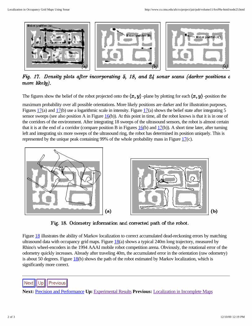
The figures show the belief of the robot projected onto the -plane by plotting for each -position the

maximum probability over all possible orientations. More likely positions are darker and for illustration purposes,Figures 17(a) and 17(b) use a logarithmic scale in intensity. Figure 17(a) shows the belief state after integrating 5sensor sweeps (see also position A in Figure 16(b)). At this point in time, all the robot knows is that it is in one ofthe corridors of the environment. After integrating 18 sweeps of the ultrasound sensors, the robot is almost certainthat it is at the end of a corridor (compare position B in Figures 16(b) and 17(b)). A short time later, after turningleft and integrating six more sweeps of the ultrasound ring, the robot has determined its position uniquely. This isrepresented by the unique peak containing 99% of the whole probability mass in Figure 17(c).

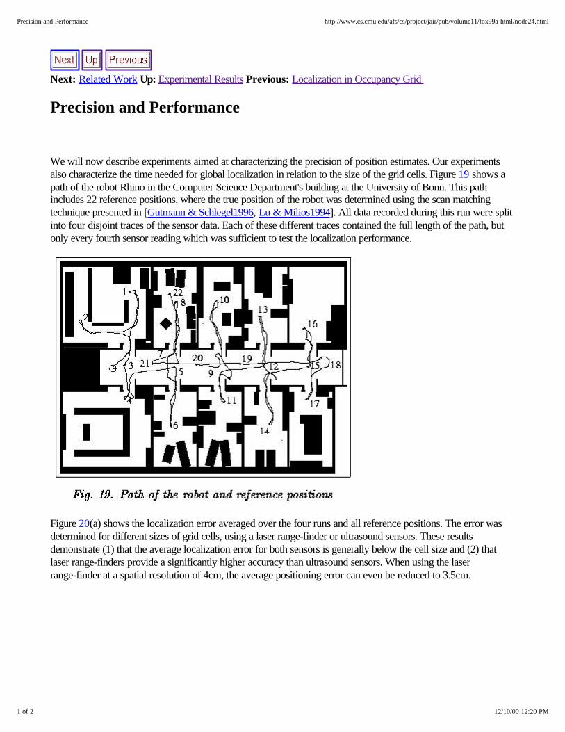
Figure 18 illustrates the ability of Markov localization to correct accumulated dead-reckoning errors by matchingultrasound data with occupancy grid maps. Figure 18(a) shows a typical 240m long trajectory, measured byRhino's wheel-encoders in the 1994 AAAI mobile robot competition arena. Obviously, the rotational error of theodometry quickly increases. Already after traveling 40m, the accumulated error in the orientation (raw odometry)is about 50 degrees. Figure 18(b) shows the path of the robot estimated by Markov localization, which issignificantly more correct.

Next: Precision and Performance Up: Experimental Results Previous: Localization in Incomplete Maps

2 of 3 12/10/00 12:19 PM

Localization in Occupancy Grid Maps Using Sonar http://www.cs.cmu.edu/afs/cs/project/jair/pub/volume11/fox99a-html/node23.html

Next: Related Work Up: Experimental Results Previous: Localization in Occupancy Grid

Precision and Performance

We will now describe experiments aimed at characterizing the precision of position estimates. Our experimentsalso characterize the time needed for global localization in relation to the size of the grid cells. Figure 19 shows apath of the robot Rhino in the Computer Science Department's building at the University of Bonn. This pathincludes 22 reference positions, where the true position of the robot was determined using the scan matchingtechnique presented in [Gutmann & Schlegel1996, Lu & Milios1994]. All data recorded during this run were splitinto four disjoint traces of the sensor data. Each of these different traces contained the full length of the path, butonly every fourth sensor reading which was sufficient to test the localization performance.

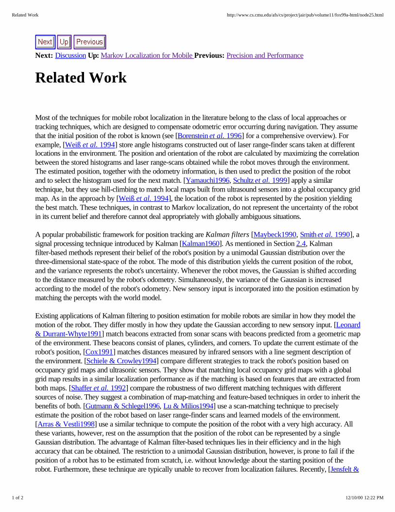
Figure 20(a) shows the localization error averaged over the four runs and all reference positions. The error wasdetermined for different sizes of grid cells, using a laser range-finder or ultrasound sensors. These resultsdemonstrate (1) that the average localization error for both sensors is generally below the cell size and (2) thatlaser range-finders provide a significantly higher accuracy than ultrasound sensors. When using the laserrange-finder at a spatial resolution of 4cm, the average positioning error can even be reduced to 3.5cm.

1 of 2 12/10/00 12:20 PM

Precision and Performance http://www.cs.cmu.edu/afs/cs/project/jair/pub/volume11/fox99a-html/node24.html

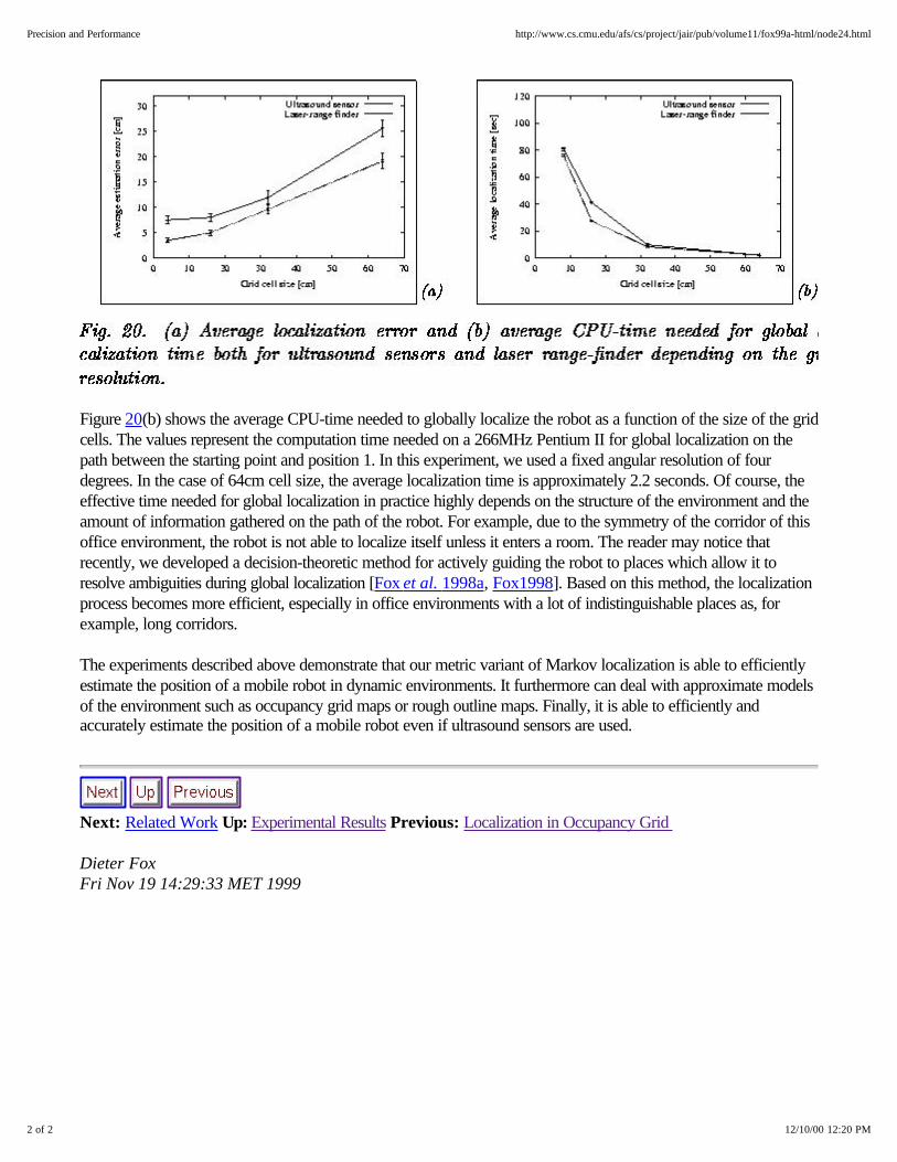
Figure 20(b) shows the average CPU-time needed to globally localize the robot as a function of the size of the gridcells. The values represent the computation time needed on a 266MHz Pentium II for global localization on thepath between the starting point and position 1. In this experiment, we used a fixed angular resolution of fourdegrees. In the case of 64cm cell size, the average localization time is approximately 2.2 seconds. Of course, theeffective time needed for global localization in practice highly depends on the structure of the environment and theamount of information gathered on the path of the robot. For example, due to the symmetry of the corridor of thisoffice environment, the robot is not able to localize itself unless it enters a room. The reader may notice thatrecently, we developed a decision-theoretic method for actively guiding the robot to places which allow it toresolve ambiguities during global localization [Fox et al. 1998a, Fox1998]. Based on this method, the localizationprocess becomes more efficient, especially in office environments with a lot of indistinguishable places as, forexample, long corridors.

The experiments described above demonstrate that our metric variant of Markov localization is able to efficientlyestimate the position of a mobile robot in dynamic environments. It furthermore can deal with approximate modelsof the environment such as occupancy grid maps or rough outline maps. Finally, it is able to efficiently andaccurately estimate the position of a mobile robot even if ultrasound sensors are used.

Next: Related Work Up: Experimental Results Previous: Localization in Occupancy Grid


2 of 2 12/10/00 12:20 PM

Precision and Performance http://www.cs.cmu.edu/afs/cs/project/jair/pub/volume11/fox99a-html/node24.html

Next: Discussion Up: Markov Localization for Mobile Previous: Precision and Performance

Related Work

Most of the techniques for mobile robot localization in the literature belong to the class of local approaches ortracking techniques, which are designed to compensate odometric error occurring during navigation. They assumethat the initial position of the robot is known (see [Borenstein et al. 1996] for a comprehensive overview). Forexample, [Weiß et al. 1994] store angle histograms constructed out of laser range-finder scans taken at differentlocations in the environment. The position and orientation of the robot are calculated by maximizing the correlationbetween the stored histograms and laser range-scans obtained while the robot moves through the environment.The estimated position, together with the odometry information, is then used to predict the position of the robotand to select the histogram used for the next match. [Yamauchi1996, Schultz et al. 1999] apply a similartechnique, but they use hill-climbing to match local maps built from ultrasound sensors into a global occupancy gridmap. As in the approach by [Weiß et al. 1994], the location of the robot is represented by the position yieldingthe best match. These techniques, in contrast to Markov localization, do not represent the uncertainty of the robotin its current belief and therefore cannot deal appropriately with globally ambiguous situations.

A popular probabilistic framework for position tracking are Kalman filters [Maybeck1990, Smith et al. 1990], asignal processing technique introduced by Kalman [Kalman1960]. As mentioned in Section 2.4, Kalmanfilter-based methods represent their belief of the robot's position by a unimodal Gaussian distribution over thethree-dimensional state-space of the robot. The mode of this distribution yields the current position of the robot,and the variance represents the robot's uncertainty. Whenever the robot moves, the Gaussian is shifted accordingto the distance measured by the robot's odometry. Simultaneously, the variance of the Gaussian is increasedaccording to the model of the robot's odometry. New sensory input is incorporated into the position estimation bymatching the percepts with the world model.

Existing applications of Kalman filtering to position estimation for mobile robots are similar in how they model themotion of the robot. They differ mostly in how they update the Gaussian according to new sensory input. [Leonard& Durrant-Whyte1991] match beacons extracted from sonar scans with beacons predicted from a geometric mapof the environment. These beacons consist of planes, cylinders, and corners. To update the current estimate of therobot's position, [Cox1991] matches distances measured by infrared sensors with a line segment description ofthe environment. [Schiele & Crowley1994] compare different strategies to track the robot's position based onoccupancy grid maps and ultrasonic sensors. They show that matching local occupancy grid maps with a globalgrid map results in a similar localization performance as if the matching is based on features that are extracted fromboth maps. [Shaffer et al. 1992] compare the robustness of two different matching techniques with differentsources of noise. They suggest a combination of map-matching and feature-based techniques in order to inherit thebenefits of both. [Gutmann & Schlegel1996, Lu & Milios1994] use a scan-matching technique to preciselyestimate the position of the robot based on laser range-finder scans and learned models of the environment.[Arras & Vestli1998] use a similar technique to compute the position of the robot with a very high accuracy. Allthese variants, however, rest on the assumption that the position of the robot can be represented by a singleGaussian distribution. The advantage of Kalman filter-based techniques lies in their efficiency and in the highaccuracy that can be obtained. The restriction to a unimodal Gaussian distribution, however, is prone to fail if theposition of a robot has to be estimated from scratch, i.e. without knowledge about the starting position of therobot. Furthermore, these technique are typically unable to recover from localization failures. Recently, [Jensfelt &

1 of 2 12/10/00 12:22 PM

Related Work http://www.cs.cmu.edu/afs/cs/project/jair/pub/volume11/fox99a-html/node25.html

Kristensen1999] introduced an approach based on multiple hypothesis tracking, which allows to modelmulti-modal probability distributions as they occur during global localization.

Markov localization, which has been employed successfully in several variants [Nourbakhsh et al. 1995, Simmons& Koenig1995, Kaelbling et al. 1996, Burgard et al. 1996, Hertzberg & Kirchner1996, Koenig &Simmons1998, Oore et al. 1997, Thrun1998a], overcomes the disadvantage of Kalman filter based techniques.The different variants of this technique can be roughly distinguished by the type of discretization used for therepresentation of the state space. [Nourbakhsh et al. 1995, Simmons & Koenig1995, Kaelbling et al. 1996] useMarkov localization for landmark-based navigation, and the state space is organized according to the topologicalstructure of the environment. Here nodes of the topological graph correspond to distinctive places in hallwayssuch as openings or junctions and the connections between these places. Possible observations of the robot are,for example, hallway intersections. The advantage of these approaches is that they can represent ambiguoussituations and thus are in principle able to globally localize a robot. Furthermore, the coarse discretization of theenvironment results in relatively small state spaces that can be maintained efficiently. The topologicalrepresentations have the disadvantage that they provide only coarse information about the robot's position and thatthey rely on the definition of abstract features that can be extracted from the sensor information. The approachestypically make strong assumptions about the nature of the environments. [Nourbakhsh et al. 1995, Simmons &Koenig1995, Kaelbling et al. 1996], for example, only consider four possible headings for the robot positionassuming that the corridors in the environment are orthogonal to each other.

Our method uses instead a fine-grained, grid-based discretization of the state space. The advantage of thisapproach compared to the Kalman filter based techniques comes from the ability to represent more complexprobability distributions. In a recent experimental comparison to the technique by [Gutmann & Schlegel1996, Lu& Milios1994], we found that Kalman filter based tracking techniques provide highly accurate position estimatesbut are less robust, since they lack the ability to globally localize the robot and to recover from localizationerrors [Gutmann et al. 1998]. In contrast to the topological implementations of Markov localization, our approachprovides accurate position estimates and can be applied even in highly unstructured environments [Burgard et al.1998a, Thrun et al. 1999]. Using the selective update scheme, our technique is able to efficiently keep track of therobot's position once it has been determined. It also allows the robot to recover from localization failures.

Finally, the vast majority of existing approaches to localization differ from ours in that they address localization instatic environments. Therefore, these methods are prone to fail in highly dynamic environments in which, forexample, large crowds of people surround the robot [Fox et al. 1998c]. However, dynamic approaches havegreat practical importance, and many envisioned application domains of service robots involve people andpopulated environments.

Next: Discussion Up: Markov Localization for Mobile Previous: Precision and Performance


2 of 2 12/10/00 12:22 PM

Related Work http://www.cs.cmu.edu/afs/cs/project/jair/pub/volume11/fox99a-html/node25.html

Next: Acknowledgment Up: Markov Localization for Mobile Previous: Related Work

Discussion

In this paper we presented a metric variant of Markov localization, as a robust technique for estimating theposition of a mobile robot in dynamic environments. The key idea of Markov localization is to maintain aprobability density over the whole state space of the robot relative to its environment. This density is updatedwhenever new sensory input is received and whenever the robot moves. Metric Markov localization representsthe state space using fine-grained, metric grids. Our approach employs efficient, selective update algorithms toupdate the robot's belief in real-time. It uses filtering to cope with dynamic environments, making our approachapplicable to a wide range of target applications.

In contrast to previous approaches to Markov localization, our method uses a fine-grained discretization of thestate space. This allows us to compute accurate position estimates and to incorporate raw sensory input into thebelief. As a result, our system can exploit arbitrary features of the environment. Additionally, our approach can beapplied in arbitrary unstructured environments and does not rely on an orthogonality assumption or similarassumptions of the existence of certain landmarks, as most other approaches to Markov localization do.

The majority of the localization approaches developed so far assume that the world is static and that the state ofthe robot is the only changing aspect of the world. To be able to localize a mobile robot even in dynamic anddensely populated environments, we developed a technique for filtering sensor measurements which are corrupteddue to the presence of people or other objects not contained in the robot's model of the environment.

To efficiently update the huge state spaces resulting from the grid-based discretization, we developed two differenttechniques. First, we use look-up operations to efficiently compute the quantities necessary to update the belief ofthe robot given new sensory input. Second, we apply the selective update scheme which focuses the computationon the relevant parts of the state space. As a result, even large belief states can be updated in real-time.

Our technique has been implemented and evaluated in several real-world experiments at different sites. Recentlywe deployed the mobile robots Rhino in the Deutsches Museum Bonn, Germany, and Minerva in theSmithsonian's National Museum of American History, Washington, DC, as interactive museum tour-guides.During these deployments, our Markov localization technique reliably estimated the position of the robots overlong periods of time, despite the fact that both robots were permanently surrounded by visitors which producedlarge amounts of false readings for the proximity sensors of the robots. The accuracy of grid-based Markovlocalization turned out to be crucial to avoid even such obstacles that could not be sensed by the robot's sensors.This has been accomplished by integrating map information into the collision avoidance system [Fox et al. 1998b].

Despite these encouraging results, several aspects warrant future research. A key disadvantage of our currentimplementation of Markov localization lies in the fixed discretization of the state space, which is always kept inmain memory. To scale up to truly large environments, it seems inevitable that one needs variable-resolutionrepresentations of the state space, such as as the one suggested in [Burgard et al. 1997, Burgard et al. 1998b,Gutmann et al. 1998]. Alternatively, one could use Monte-Carlo based representations of the state space asdescribed in [Fox et al. 1999]. Here, the robot's belief is represented by samples that concentrate on the mostlikely parts of the state space.

1 of 2 12/10/00 12:23 PM

Discussion http://www.cs.cmu.edu/afs/cs/project/jair/pub/volume11/fox99a-html/node26.html

Next: References Up: Markov Localization for Mobile Previous: Discussion

AcknowledgmentThe authors would like to thank the research group for autonomous intelligent systems at the University of Bonnfor fruitful discussions, useful suggestions and comments, especially Daniel Hennig and Andreas Derr. We wouldalso like to thank the members of CMU's Robot Learning Lab for many inspiring discussions. Finally, we wouldlike to thank the staff of the Deutsches Museum Bonn and the National Museum of American History for theirenthusiasm and their willingness to expose their visitors to one of our mobile robots.

This research is sponsored in part by NSF (CAREER Award IIS-9876136) and DARPA via TACOM (contractnumber DAAE07-98-C-L032), and Rome Labs (contract number F30602-98-2-0137), which is gratefullyacknowledged. The views and conclusions contained in this document are those of the authors and should not beinterpreted as necessarily representing official policies or endorsements, either expressed or implied, of NSF,DARPA, TACOM, Rome Labs, or the United States Government.


1 of 1 12/10/00 12:23 PM

Acknowledgment http://www.cs.cmu.edu/afs/cs/project/jair/pub/volume11/fox99a-html/node27.html

Documents

Markov Localization for Mobile Robots in Dynamic …biorobotics.ri.cmu.edu/papers/sbp_papers/integrated4/burgard_bayes... · Localization, that is the estimation of a robot's location