Embed Size (px)
Citation preview

Markov Functional Model
Peter Caspers
IKB
November 13, 2013
Peter Caspers (IKB) Markov Functional Model November 13, 2013 1 / 72

Disclaimer
The contents of this presentation are the sole and personal opinion of theauthor and do not express IKB’s opinion on any subject presented in thefollowing.
Peter Caspers (IKB) Markov Functional Model November 13, 2013 2 / 72

Table of contents
1 Code Example
2 Theoretical Background
3 Model description
4 Calibration
5 Numerics
6 Secondary instrument set calibration
7 Implementation in QuantLib
8 References
9 Questions
Peter Caspers (IKB) Markov Functional Model November 13, 2013 3 / 72

Code Example
Term Sheet
Consider the following interest rate swap, with 10y maturity.
We receive yearly coupons of type EUR CMS 10y
We pay Euribor 6m + 26.7294bp
We are short a bermudan yearly call right
What is a suitable way to price this deal ?
Peter Caspers (IKB) Markov Functional Model November 13, 2013 4 / 72

Code Example
Model requirements
A good start1 would be to use a model that
prices the underlying CMS coupons consistently with given swaptionvolatility smiles
can in addition be calibrated to swaptions representing the call right(say for the moment to atm coterminals)
gives us control over intertemporal correlations
A plain Hull White model fulfills #2 and #3 but clearly fails to meet #1.
1one important requirement - the decorrelation of Euribor6m and CMS10yrates - is missing here, and actually not satisfied by the Markov 1F model
Peter Caspers (IKB) Markov Functional Model November 13, 2013 5 / 72

Code Example
The Markov model approach
This is where the Markov Functional Model jumps in. Before going intodetails on how it works, we give an example in terms of QuantLib Code.Let’s suppose you have already constructed aHandle<YieldTermStructure> yts
representing a 6m swap curve and aHandle<SwaptionVolatilityStructure> swaptionVol
representing a swaption volatility cube (suitable for CMS coupons pricing).
Peter Caspers (IKB) Markov Functional Model November 13, 2013 6 / 72

Code Example
Model construction
We create a markov model instance as followsboost::shared_ptr<MarkovFunctional> markov(
new MarkovFunctional(yts,reversion,sigmaSteps,sigma,
swaptionVol,cmsFixingDates,
cmsTenors,swapIndexBase));
with a mean reversionReal reversion
controlling intertemporal correlations (see below), a piecewise volatility(for the coterminal calibraiton) given bystd::vector<Date> sigmaSteps
std::vector<Real> sigma
Peter Caspers (IKB) Markov Functional Model November 13, 2013 7 / 72

Code Example
Model construction (ctd)
our structured coupon fixing dates and tenorsstd::vector<Date> cmsFixingDates
std::vector<Period> cmsTenors
and a swap indexboost::shared_ptr<SwapIndex> swapIndexBase
codifying the conventions of our cms coupons.
Peter Caspers (IKB) Markov Functional Model November 13, 2013 8 / 72
Code Example
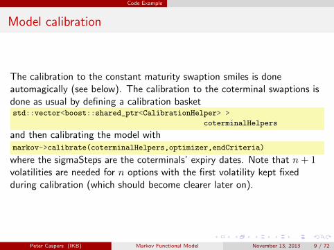
Model calibration
The calibration to the constant maturity swaption smiles is doneautomagically (see below). The calibration to the coterminal swaptions isdone as usual by defining a calibration basketstd::vector<boost::shared_ptr<CalibrationHelper> >
coterminalHelpers
and then calibrating the model withmarkov->calibrate(coterminalHelpers,optimizer,endCriteria)
where the sigmaSteps are the coterminals’ expiry dates. Note that n+ 1volatilities are needed for n options with the first volatility kept fixedduring calibration (which should become clearer later on).
Peter Caspers (IKB) Markov Functional Model November 13, 2013 9 / 72

Code Example
Instrument
Our callable swap is represented as two instruments, the swap without thecall right and the call right itself. The former can be constructed asboost::shared_ptr<FloatFloatSwap> swap(new FloatFloatSwap( ... ));
and the latter as a swaptionboost::shared_ptr<FloatFloatSwap>
underlying(new FloatFloatSwap( ... ));
boost::shared_ptr<Exercise>
exercise(new BermudanExercise(exerciseDates));
boost::shared_ptr<FloatFloatSwaption>
swaption(new FloatFloatSwaption(underlying, exercise));
Peter Caspers (IKB) Markov Functional Model November 13, 2013 10 / 72

Code Example
Pricing Engine
To do the actual pricing we need a suitable pricing engine which can beconstructed byboost::shared_ptr<PricingEngine>
engine(new Gaussian1dFloatFloatSwaptionEngine(markov));
and assigned to our instrument by means ofswaption->setPricingEngine(engine);
which then allows to extract the dirty npvReal npv = swaption->NPV();
The npv of the swap on the other hand can be retrieved with standard cmscoupon pricers implementing a replication in some swap rate model 2.
2this is slightly different from pricing the full structured swap in the markovmodel, since there are theoretical differences between the models (in addition todifferences in their numerical solution)
Peter Caspers (IKB) Markov Functional Model November 13, 2013 11 / 72
Code Example
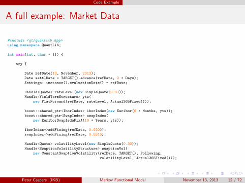
A full example: Market Data
#include <ql/quantlib.hpp>
using namespace QuantLib;
int main(int, char * []) {
try {
Date refDate(13, November, 2013);
Date settlDate = TARGET().advance(refDate, 2 * Days);
Settings::instance().evaluationDate() = refDate;
Handle<Quote> rateLevel(new SimpleQuote(0.03));
Handle<YieldTermStructure> yts(
new FlatForward(refDate, rateLevel, Actual365Fixed()));
boost::shared_ptr<IborIndex> iborIndex(new Euribor(6 * Months, yts));
boost::shared_ptr<SwapIndex> swapIndex(
new EuriborSwapIsdaFixA(10 * Years, yts));
iborIndex->addFixing(refDate, 0.0200);
swapIndex->addFixing(refDate, 0.0315);
Handle<Quote> volatilityLevel(new SimpleQuote(0.30));
Handle<SwaptionVolatilityStructure> swaptionVol(
new ConstantSwaptionVolatility(refDate, TARGET(), Following,
volatilityLevel, Actual365Fixed()));
Peter Caspers (IKB) Markov Functional Model November 13, 2013 12 / 72

Code Example
A full example: Cms Swap and Exercise Schedule
Date termDate = TARGET().advance(settlDate, 10 * Years);
Schedule sched1(settlDate, termDate, 1 * Years, TARGET(),
ModifiedFollowing, ModifiedFollowing,
DateGeneration::Forward, false);
Schedule sched2(settlDate, termDate, 6 * Months, TARGET(),
ModifiedFollowing, ModifiedFollowing,
DateGeneration::Forward, false);
Real nominal = 100000.0;
boost::shared_ptr<FloatFloatSwap> cmsswap(new FloatFloatSwap(
VanillaSwap::Payer, nominal, nominal, sched1, swapIndex,
Thirty360(), sched2, iborIndex, Actual360(),
false,false,1.0,0.0,Null<Real>(),Null<Real>(),1.0,0.00267294));
std::vector<Date> exerciseDates;
std::vector<Date> sigmaSteps;
std::vector<Real> sigma;
sigma.push_back(0.01);
for (Size i = 1; i < sched1.size() - 1; i++) {
exerciseDates.push_back(swapIndex->fixingDate(sched1[i]));
sigmaSteps.push_back(exerciseDates.back());
sigma.push_back(0.01);
}
Peter Caspers (IKB) Markov Functional Model November 13, 2013 13 / 72
Code Example
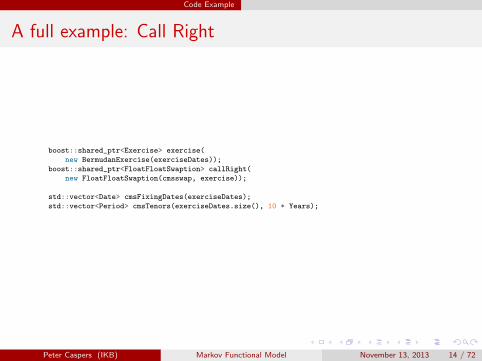
A full example: Call Right
boost::shared_ptr<Exercise> exercise(
new BermudanExercise(exerciseDates));
boost::shared_ptr<FloatFloatSwaption> callRight(
new FloatFloatSwaption(cmsswap, exercise));
std::vector<Date> cmsFixingDates(exerciseDates);
std::vector<Period> cmsTenors(exerciseDates.size(), 10 * Years);
Peter Caspers (IKB) Markov Functional Model November 13, 2013 14 / 72

Code Example
A full example: Models and Engines
Handle<Quote> reversionLevel(new SimpleQuote(0.02));
boost::shared_ptr<NumericHaganPricer> haganPricer(
new NumericHaganPricer(swaptionVol,
GFunctionFactory::NonParallelShifts,
reversionLevel));
setCouponPricer(cmsswap->leg(0), haganPricer);
boost::shared_ptr<MarkovFunctional> mf(new MarkovFunctional(
yts, reversionLevel->value(), sigmaSteps, sigma, swaptionVol,
cmsFixingDates, cmsTenors, swapIndex));
boost::shared_ptr<Gaussian1dFloatFloatSwaptionEngine> floatEngine(
new Gaussian1dFloatFloatSwaptionEngine(mf));
callRight->setPricingEngine(floatEngine);
Peter Caspers (IKB) Markov Functional Model November 13, 2013 15 / 72

Code Example
A full example: Calibration Basket
boost::shared_ptr<SwapIndex> swapBase(
new EuriborSwapIsdaFixA(30 * Years, yts));
std::vector<boost::shared_ptr<CalibrationHelper> > basket =
callRight->calibrationBasket(swapBase, *swaptionVol,
BasketGeneratingEngine::Naive);
boost::shared_ptr<Gaussian1dSwaptionEngine> stdEngine(
new Gaussian1dSwaptionEngine(mf));
for (Size i = 0; i < basket.size(); i++)
basket[i]->setPricingEngine(stdEngine);
Peter Caspers (IKB) Markov Functional Model November 13, 2013 16 / 72
Code Example
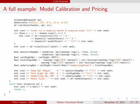
A full example: Model Calibration and Pricing
LevenbergMarquardt opt;
EndCriteria ec(2000, 500, 1E-8, 1E-8, 1E-8);
mf->calibrate(basket, opt, ec);
std::cout << "model vol & swaption market & swaption model \\\\" << std::endl;
for (Size i = 0; i < basket.size(); i++) {
std::cout << mf->volatility()[i] << " & "
<< basket[i]->marketValue() << " & "
<< basket[i]->modelValue() << " \\\\" << std::endl;
}
std::cout << mf->volatility().back() << std::endl;
Real analyticSwapNpv = CashFlows::npv(cmsswap->leg(1), **yts, false) -
CashFlows::npv(cmsswap->leg(0), **yts, false);
Real callRightNpv = callRight->NPV();
Real firstCouponNpv = - cmsswap->leg(0)[0]->amount() * yts->discount(cmsswap->leg(0)[0]->date()) +
cmsswap->leg(1)[0]->amount() * yts->discount(cmsswap->leg(1)[0]->date());
Real underlyingNpv = callRight->result<Real>("underlyingValue") + firstCouponNpv;
std::cout << "Swap Npv (Hagan) & " << analyticSwapNpv << "\\\\" << std::endl;
std::cout << "Call Right Npv (MF) & " << callRightNpv << "\\\\" << std::endl;
std::cout << "Underlying Npv (MF) & " << underlyingNpv << "\\\\" << std::endl;
std::cout << "Model trace : " << std::endl << mf->modelOutputs() << std::endl;
}
catch (std::exception &e) {
std::cerr << e.what() << std::endl;
return 1;
}
}
Peter Caspers (IKB) Markov Functional Model November 13, 2013 17 / 72
Code Example
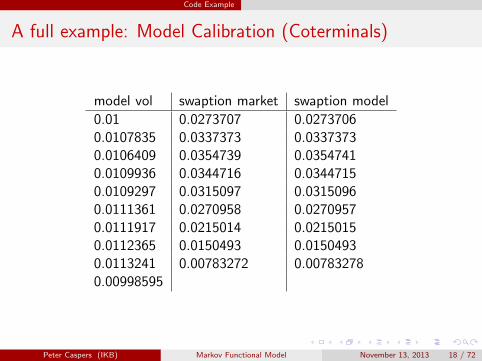
A full example: Model Calibration (Coterminals)
model vol swaption market swaption model
0.01 0.0273707 0.02737060.0107835 0.0337373 0.03373730.0106409 0.0354739 0.03547410.0109936 0.0344716 0.03447150.0109297 0.0315097 0.03150960.0111361 0.0270958 0.02709570.0111917 0.0215014 0.02150150.0112365 0.0150493 0.01504930.0113241 0.00783272 0.007832780.00998595
Peter Caspers (IKB) Markov Functional Model November 13, 2013 18 / 72
Code Example
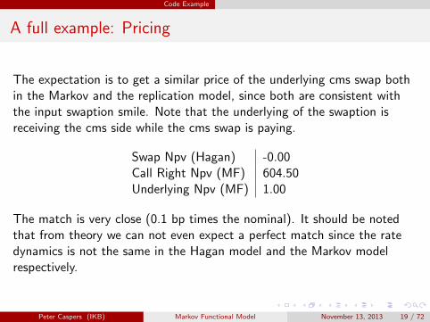
A full example: Pricing
The expectation is to get a similar price of the underlying cms swap bothin the Markov and the replication model, since both are consistent withthe input swaption smile. Note that the underlying of the swaption isreceiving the cms side while the cms swap is paying.
Swap Npv (Hagan) -0.00Call Right Npv (MF) 604.50Underlying Npv (MF) 1.00
The match is very close (0.1 bp times the nominal). It should be notedthat from theory we can not even expect a perfect match since the ratedynamics is not the same in the Hagan model and the Markov modelrespectively.
Peter Caspers (IKB) Markov Functional Model November 13, 2013 19 / 72
Code Example
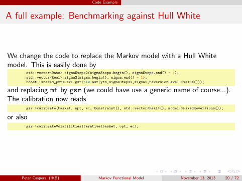
A full example: Benchmarking against Hull White
We change the code to replace the Markov model with a Hull Whitemodel. This is easily done by
std::vector<Date> sigmaSteps2(sigmaSteps.begin(), sigmaSteps.end() - 1);
std::vector<Real> sigma2(sigma.begin(), sigma.end() - 1);
boost::shared_ptr<Gsr> gsr(new Gsr(yts,sigmaSteps2,sigma2,reversionLevel->value()));
and replacing mf by gsr (we could have use a generic name of course...).The calibration now reads
gsr->calibrate(basket, opt, ec, Constraint(), std::vector<Real>(), model->FixedReversions());
or alsogsr->calibrateVolatilitiesIterative(basket, opt, ec);
Peter Caspers (IKB) Markov Functional Model November 13, 2013 20 / 72

Code Example
A full example: Pricing in the Hull White model
The fit to the coterminals is exact, just as above (with different modelvolatilities of course). The pricing compares ot the Markov model asfollows:
Swap Npv (Hagan) -0.00 -0.00
Markov Hull White
Call Right Npv 604.50 1012Underlying Npv 1.00 657.81
The underlying and the option are drastically overpriced (both) by over60bp in the Hull White model.
Peter Caspers (IKB) Markov Functional Model November 13, 2013 21 / 72

Code Example
A full example: A more realistic smile surface
Swaption smiles are usually far from being flat. We test the model with aSABR volatility cube (with constant parameters α = 0.15, β = 0.80,ν = 0.20, ρ = −0.30) by setting
Handle<SwaptionVolatilityStructure> swaptionVol(
new SingleSabrSwaptionVolatility(refDate, TARGET(), Following, 0.15,
0.80, -0.30, 0.20,
Actual365Fixed(), swapIndex));
Swap Npv (Hagan) 246.00 246.00
Markov Hull White
Call Right Npv 696.96 1004.79Underlying Npv 259.96 648.26
Again the underlying and the option is overpriced (by 40bp resp. 53bp) inthe Hull White model. In the Markov model the fit is still good (1.4bpunderlying price difference).
Peter Caspers (IKB) Markov Functional Model November 13, 2013 22 / 72
Code Example
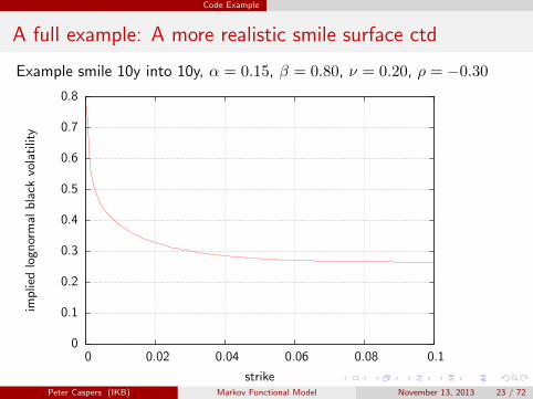
A full example: A more realistic smile surface ctd
Example smile 10y into 10y, α = 0.15, β = 0.80, ν = 0.20, ρ = −0.30
0
0.1
0.2
0.3
0.4
0.5
0.6
0.7
0.8
0 0.02 0.04 0.06 0.08 0.1
imp
lied
logn
orm
alb
lack
vola
tilit
y
strikePeter Caspers (IKB) Markov Functional Model November 13, 2013 23 / 72

Code Example
A full example: Model diagnostics
The markov model can generate information on the calibration processwithstd::cout << "Model trace : " << std::endl << mf->modelOutputs()
<< std::endl;
The output contains information on
numerical model parameters
settings for smile preconditioning
yield term structure calibration results
volatility smile calibration results
and can help identifying calibration problems, resp. confirm a successfulcalibration.
Peter Caspers (IKB) Markov Functional Model November 13, 2013 24 / 72

Code Example
A full example: Model diagnostics (model parameters /smile settings)
Markov functional model trace output
Model settings
Grid points y : 64
Std devs y : 7
Lower rate bound : 0
Upper rate bound : 2
Gauss Hermite points : 32
Digital gap : 1e-05
Adjustments : Kahale SmileExp
Smile moneyness checkpoints:
Peter Caspers (IKB) Markov Functional Model November 13, 2013 25 / 72

Code Example
A full example: Model diagnostics (yield term structure fit)
The raw outputYield termstructure fit:
expiry;tenor;atm;annuity;digitalAdj;ytsAdj;marketzerorate;modelzerorate;diff(bp)
November 13th, 2014;10Y;0.03047961644430512;8.267635590910791;1;1;0.03000000000000008;0.03008016185429107;-0.8016185429099432
November 12th, 2015;10Y;0.0304803836917478;8.023747530203391;1;1;0.02999999999999999;0.03003959599137232;-0.395959913723383
[...]
is meant to be analyzed in another application like office
Peter Caspers (IKB) Markov Functional Model November 13, 2013 26 / 72

Code Example
A full example: Model diagnostics (volatility smile fit)
Peter Caspers (IKB) Markov Functional Model November 13, 2013 27 / 72

Theoretical Background
Axiomatic Hull White
Any gaussian one factor HJM model which satisfies separability, i.e.
σf (t, T ) = g(t)h(T ) (1)
for the instantaneous forward rate volatility with deterministic g, h > 0,necessarily fulfills
dr(t) = (θ(t)− a(t)r(t))dt+ σ(t)dW (t) (2)
for the short rate r, which means, it is a Hull White one factor model.
Peter Caspers (IKB) Markov Functional Model November 13, 2013 28 / 72

Theoretical Background
The T-forward numeraire
Set x(t) := r(t)− f(0, t) and fix a horizon T , then in the T -forwardmeasure the numeraire can be written
N(t) = P (t, T ) =P (0, T )
P (0, t)e−x(t)A(t,T )+B(t,T ) (3)
with A,B dependent on the model parameters. The Hull White model iscalled an affine model.
Peter Caspers (IKB) Markov Functional Model November 13, 2013 29 / 72
Theoretical Background
Smile in the Hull White Model
The distribution of N(t) is lognormal. The shape of the distributioncan not be controlled by any of the model parameters.
For fixed t you can calibrate the model to one market quoted interestrate optoin (typically a caplet or swaption).
You can choose the strike of the option, but the rest of the smile isimplied by the model.
Peter Caspers (IKB) Markov Functional Model November 13, 2013 30 / 72

Theoretical Background
Callable vanilla swaps
Pricing of callable fix versus Libor swaps may be done in a Hull Whitemodel which is calibrated as follows:
For each call date find a market quoted swaption which is equivalentto the call right (in some sense, e.g. by matching the npv and its firstand second derivative of the underlying at E(x(t))).
Calibrate the volatility function σ(t) to match the basket of theseswaptions.
Choose the mean reversion of the model to control serial correlations.
Peter Caspers (IKB) Markov Functional Model November 13, 2013 31 / 72
Theoretical Background
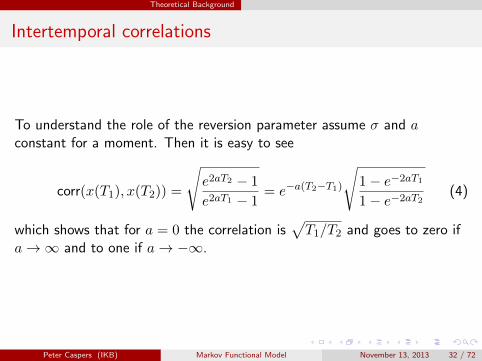
Intertemporal correlations
To understand the role of the reversion parameter assume σ and aconstant for a moment. Then it is easy to see
corr(x(T1), x(T2)) =
√e2aT2 − 1
e2aT1 − 1= e−a(T2−T1)
√1− e−2aT1
1− e−2aT2(4)
which shows that for a = 0 the correlation is√T1/T2 and goes to zero if
a→∞ and to one if a→ −∞.
Peter Caspers (IKB) Markov Functional Model November 13, 2013 32 / 72
Theoretical Background
Callable cms swaps
The calll rights in a callable cms swap are options on a swap exchangingcms coupons against fix or Libor rates. Such underlying swaps aredrastically mispriced in the Hull White model in general.
cms coupons are replicated using swaptions covering the whole strikecontinuum (0,∞)
The swaption smile in the Hull White model is generally notconsistent with the market smile and so are the prices of cms coupons
Obviously we need a more flexible model to price such structures
Peter Caspers (IKB) Markov Functional Model November 13, 2013 33 / 72
Theoretical Background
Model requirements
The wishlist for the model is as follows
We want to be capable of calibrating to a whole smile of (constantmaturity) swaptions, not only to one strike, for all fixing dates of thecms coupons. This is to match the coupons of the underlying.
In addition we would like to calibrate to (possibly strike / maturityadjusted) coterminal swaptions to match the options representing thecall rights.
Finally we need some control over intertemporal correlations, i.e.something operating like the reversion parameter in the Hull Whitemodel
The idea to do so is to relax the functional dependency between the statevariable x and the numeraire N(t, x).
Peter Caspers (IKB) Markov Functional Model November 13, 2013 34 / 72

Model description
The driving process
We start with a markov process driving the dynamics of the model asfollows:
dx = σ(t)eatdW (t) (5)
and x(0) = 0. The intertemporal correlation of the state variable x is thesame as for the Hull White model, see (4), i.e. the parameter a can beused to control the correlation just as the reversion parameter in the HullWhite model.
Peter Caspers (IKB) Markov Functional Model November 13, 2013 35 / 72

Model description
The numeraire surface
The model is operated in the T -forward measure, T chosen big enough tocover all cashflows relevant for the actual pricing under consideration. Thelink between the state x(t) and the numeraire P (t, T ) is given by
P (t, T, x) = N(t, x) (6)
which we allow to be a non parametric surface to have maximum flexibilityin calibration.
Peter Caspers (IKB) Markov Functional Model November 13, 2013 36 / 72

Calibration
Calibrating the numeriare surface to market smiles
The price of a digital swaption paying out an annuity A(t) on expiry t ifthe swap rate S(t) ≥ K in our model is
digmodel = P (0, T )
∫ ∞y∗
A(t, y)
P (t, T )φ(y)dy (7)
where y∗ is the strike in the normalized state variable space (thecorrespondence between y and S(t) is constructed to be monotonic).
Peter Caspers (IKB) Markov Functional Model November 13, 2013 37 / 72

Calibration
Implying the swap rate
Given the market smile of S(t) we can compute the market pricedigmkt(K) of digitals for strikes K. For given y∗ we can solve the equation
digmkt(K) = P (0, T )
∫ ∞y∗
A(t, y)
P (t, T )φ(y)dy (8)
for K to find the swap rate corresponding to the state variable value y∗.For this digmkt(·) should be a monotonic function whose image is equal tothe possible digital prices (0, A(0)]. We will revisit this later.
Peter Caspers (IKB) Markov Functional Model November 13, 2013 38 / 72
Calibration
Computing the deflated annuity
To compute the deflated annuity
A(t)
P (t, T )=
n∑k=1
τkP (t, tk)
P (t, T )(9)
we observe that
P (t, u)
P (t, T )
∣∣∣∣y(t)
= E
(1
P (u, T )
∣∣∣∣y(t)) (10)
i.e. we have to integrate the reciprocal of the numeraire at future times.Working backward in time we can assume that we know the numeraire atthese times (starting with N(T ) ≡ 1).
Peter Caspers (IKB) Markov Functional Model November 13, 2013 39 / 72

Calibration
Converting swap rate to numeraire
Having computed the swap rate S(t) we have to convert this value to anumeraire value N(t). Since
S(t)A(t) + P (t, t∗) = 1 (11)
we get (by division by N(t))
N(t) =1
S(t)A(t)N(t) +
P (t,t∗)N(t)
(12)
all terms on the right hand side computable via deflated zerobonds asshown above. Note that we use a slightly modified swap rate here, namelyone without start delay.
Peter Caspers (IKB) Markov Functional Model November 13, 2013 40 / 72
Calibration
Calibration to a second instrument set
Up to now we have not made use of the volatility σ(t) in the drivingmarkov process of the model. This parameter can be used to calibrate themodel to a second instrument set, however only a single strike can bematched obviously for each expiry. A typical set up would be
calibrate the numeraire to an underlying rate smile, e.g. constantmaturity swaptions for cms coupon pricing
calibrate σ(t) to (standard atm or possibly adjusted) coterminalswaptions for call right calibration
Note that after changing σ(t) the numeraire surface needs to be updated,too.
Peter Caspers (IKB) Markov Functional Model November 13, 2013 41 / 72
Calibration
Input smile preconditioning
To ensure a bijective mapping
digmkt : (0,∞)→ (0, A(0)) (13)
it is sufficient to have an arbitrage free input smile with a C1 call pricefunction. It is possible to allow for negative rates and generalize theinterval (0,∞) to (−κ,∞) with some suitable κ > 0, e.g. κ = 1%. Ingeneral input smiles are not arbitrage free, so some preconditioning isadvisable, since arbitrageable smiles will break the numeraire calibration.
Peter Caspers (IKB) Markov Functional Model November 13, 2013 42 / 72
Calibration
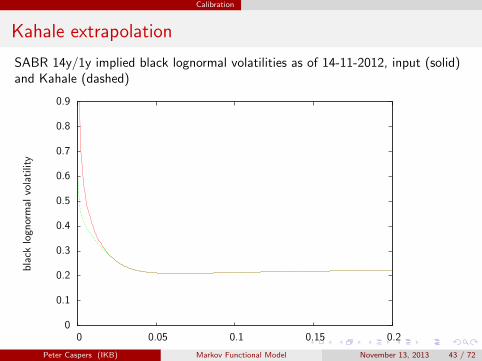
Kahale extrapolation
SABR 14y/1y implied black lognormal volatilities as of 14-11-2012, input (solid)and Kahale (dashed)
0
0.1
0.2
0.3
0.4
0.5
0.6
0.7
0.8
0.9
0 0.05 0.1 0.15 0.2
bla
cklo
gnor
mal
vola
tilit
y
strikePeter Caspers (IKB) Markov Functional Model November 13, 2013 43 / 72
Calibration
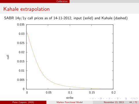
Kahale extrapolation
SABR 14y/1y call prices as of 14-11-2012, input (solid) and Kahale (dashed)
0
0.005
0.01
0.015
0.02
0.025
0.03
0.035
0 0.05 0.1 0.15 0.2
call
strike
Peter Caspers (IKB) Markov Functional Model November 13, 2013 44 / 72
Calibration
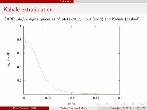
Kahale extrapolation
SABR 14y/1y digital prices as of 14-11-2012, input (solid) and Kahale (dashed)
0
0.2
0.4
0.6
0.8
1
0 0.05 0.1 0.15 0.2
dig
ital
call
strike
Peter Caspers (IKB) Markov Functional Model November 13, 2013 45 / 72
Calibration
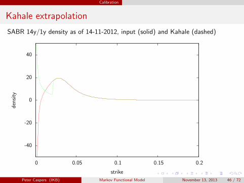
Kahale extrapolation
SABR 14y/1y density as of 14-11-2012, input (solid) and Kahale (dashed)
-40
-20
0
20
40
0 0.05 0.1 0.15 0.2
den
sity
strike
Peter Caspers (IKB) Markov Functional Model November 13, 2013 46 / 72

Numerics
Interpolation of the numeraire
In a numerical implementation of the model we will need to discretize thenumeraire surface on a grid (ti, yj).
in y-direction we interpolate N(t, y) (normalized by todays marketforward numeraire) with monotonic cubic splines with Lagrange endcondition. Outside a range of specified standard deviations (defaultedto 7), we extrapolate flat.
in t-direction we interpolate the reciprocal of the normalizednumeraire linearly. This ensures a perfect match of todays input yieldcurve even for interpolated times as can easily be seen from (10).After the horizon T we extrapolate flat (N ≡ 1 there anyway), onlyfor technical reasons.
Peter Caspers (IKB) Markov Functional Model November 13, 2013 47 / 72

Numerics
Sample numeraire surface
Numeraire surface for market data as of 14-11-2012
02468101214
-3-2
-10
12
3
0
0.2
0.4
0.6
0.8
1
N(t,y)
t
y
N(t,y)
0.30.40.50.60.70.80.911.1
Peter Caspers (IKB) Markov Functional Model November 13, 2013 48 / 72

Numerics
Interpolation of payoffs
Payoffs occuring in the numeraire bootstrap (digitals) or later in pricingexotics are also interpolated with Lagrange splines. We leave it as anoption to
restrict to integration of the payoff to a specified number of standarddeviations,
extrapolate the payoff flat
extrapolate the payoff according to the Lagrange end condition
The results should not depend significantly on this choice, otherwise thenumerical parameters should be increased.
Peter Caspers (IKB) Markov Functional Model November 13, 2013 49 / 72
Numerics
Numerical Integration for deflated zero bonds
To compute deflated zerobond prices according to (10) it turns out that itis fast and accurate to
use the celebrated Gauss Hermite Integration scheme where
32 points are more than enough usually to ensure a good accuracy.
This is because the integrand is globally well approximated by polynomials.
Peter Caspers (IKB) Markov Functional Model November 13, 2013 50 / 72

Numerics
Numerical Integration for payoffs
For the numerical integration of
digitals during numeraire bootstrapping or
exotic pricing
Gauss Hermite is possible but not leading to satisfactory accuracy. This isdue to the non global nature of the integrand in this case. Here we rely onexact integration of the piecewise 3rd order polynomials against thegaussian density, which is possible in closed form only involving the errorfunction erf
Peter Caspers (IKB) Markov Functional Model November 13, 2013 51 / 72

Numerics
How is the yield curve matched after all ?
It is interesting to note that the initial yield curve is matched bycalibrating the numeraire to market input smiles. The yield curve is nevera direct input though, as it is e.g. for the Hull White model. It isreconstructed by the model via the numeraire density coded in and readoff the market smile during numeraire bootstrapping.
Peter Caspers (IKB) Markov Functional Model November 13, 2013 52 / 72

Numerics
Long term constant maturity calibration
The hardest case of calibration is a long term calibration to constantmaturity swaptions (or caplets).
We start at maturity T and bootstrap the numeraire at some tk < T ,introducing some numerical noise in N(tk).
We then boostrap N(tk−1) for tk−1 < tk, relying on the alreadybootstrapped future numeraire values.
In case of a coterminal calibration we largely still use N(T ) andN(tk) only to a smaller degree.
In case of cm calibration however we have to rely on N(tk) with tknearer to our calibration time t.
Therefore in long term cm calibration numerical noise may pile up givinglarge errors for the shorter term numeraire surface.
Peter Caspers (IKB) Markov Functional Model November 13, 2013 53 / 72

Numerics
Yield curve match with standard numerical parameters
Fit to Yts flat @ 3%, 2y cm swaptions @ 20%, 7 standard deviations, 200 % upper rate bound
0.029
0.0292
0.0294
0.0296
0.0298
0.03
0.0302
0.0304
0.0306
0.0308
0.031
0 10 20 30 40 50
zero
rate
maturity
Peter Caspers (IKB) Markov Functional Model November 13, 2013 54 / 72

Numerics
Increasing numerical accuracy for long term cm baskets
The first idea in this case is to increase the numerical accuracy byincreasing
the number of covered standard deviations (e.g. from 7 to 12)
the upper cut off point for rates (e.g. from 200% to 400%)
(maybe the number of discretization points, though less critical)
However this breaks the calibration totally, because the standard(”double”) 53 bit mantissa numerical precision is not sufficient to do thecomputations numerically stable any more.
Peter Caspers (IKB) Markov Functional Model November 13, 2013 55 / 72
Numerics
NTL high precision computing
The NTL and boost libraries provide support for arbitrary floating pointprecision. We incorporated NTL support as an option replacing thestandard double precision by an arbitrary mantissa length precision in thecritical sections of the computation (which turned out to be the integrationof payoffs against the gaussian density, where large integrand values aremultiplied by small density values). NTL is activated by commenting out
// uncomment to enable NTL support
#define GAUSS1D_ENABLE_NTL
in gaussian1dmodel.hpp. The mantissa length is then set (e.g. to113bit) with
boost::math::ntl::RR:SetPrecision(113)
Peter Caspers (IKB) Markov Functional Model November 13, 2013 56 / 72

Numerics
Yield curve match using high precision computing
Fit to Yts flat @ 3%, 2y cm swaptions @ 20%, 150bit mantissa, 12 standard deviations, 400 % upper rate bound
0.02999
0.029992
0.029994
0.029996
0.029998
0.03
0.030002
0.030004
0.030006
0.030008
0.03001
0 10 20 30 40 50
zero
rate
maturity
Peter Caspers (IKB) Markov Functional Model November 13, 2013 57 / 72
Numerics
A more pragmatic approach: Adjustment factors
Computations with NTL are slow. A more practical way to stabilize thecalibration in difficult circumstances are adjustment factors forcing thenumeraire to match the market input yield curve. The adjustment factor isintroduced by replacing
N(ti, yj)→ N(ti, yj)Pmodel(0, ti)
Pmarket(0, ti)(14)
This option should be used with some care because it may lower theaccuracy of the volatility smile match. In most situations the adjustmentfactors are moderate though, in the example we had before:
Peter Caspers (IKB) Markov Functional Model November 13, 2013 58 / 72

Numerics
Adjustment factors in the example above
Date Adjustment Factor
November 14th, 2013 1.00000029079227November 14th, 2014 0.999999566861981November 14th, 2015 0.999999720414697November 14th, 2016 0.999999838009949November 14th, 2017 0.999999380770489... ...November 14th, 2056 0.999804362556495November 14th, 2057 0.999904959217797November 14th, 2058 0.99988000473961November 14th, 2059 0.999816723715493November 14th, 2060 0.999830021528368November 14th, 2061 0.999737006370401November 14th, 2062 0.999761860227793November 14th, 2063 0.999887598113548
Peter Caspers (IKB) Markov Functional Model November 13, 2013 59 / 72

Numerics
MarkovFunctional Options - Numerical Parameters
yGridPoint Number of discretization points for normalized statevariable (default 64)
yStdDevs Number of standard deviations of normalized state variablecovered (default 7)
gaussHermitePoints Number of points used in Gauss hermiteintegration (default 32)
digitalGap Numerical stepsize to compute market digitals from callspreads (default 10−5)
marketRateAccuracy Accuracy (in model swap rate) when matchingmarket digitals (default 10−7)
lowerRateBound Lower bound for model’s (underlying) rates (default0%)
upperRateBound Upper bound for model’s (underlying) rates(default 200%)
Peter Caspers (IKB) Markov Functional Model November 13, 2013 60 / 72
Numerics
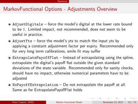
MarkovFunctional Options - Adjustments Overview
AdjustDigitals – force the model’s digital at the lower rate boundto be 1. Limited impact, not recommended, does not seem to beuseful in practice.
AdjustYts – force the model’s yts to match the input yts byapplying a constant adjustment factor per expiry. Recommended onlyfor very long term calibrations, smile fit may suffer
ExtrapolatePayoffFlat – Instead of extrapolating using the spline,extrapolate the digital’s payoff flat outside the given standarddeviations of the state variable. Recommended only for sanity checks,should have no impact, otherwise numerical parameters have to beadjusted
NoPayoffExtrapolation – Do not extrapolate the payoff at all.Same as for ExtrapolatePayoffFlat holds
Peter Caspers (IKB) Markov Functional Model November 13, 2013 61 / 72

Numerics
MarkovFunctional Options - Adjustments Overview ctd.
KahaleSmile – Use Kahale smile preconditioning on arbitrageablewings, recommended (or SabrSmile) unless you are sure to providean arbitrage free smile input
KahaleInterpolation – Use Kahale smile interpolation (impliesKahaleSmile), for naively interpolated smiles (linear, ...), howevergenerates “Bat Man shaped” Densities, not recommended unlessSabrSmile fails to work or is too inaccurate w.r.t. fit
SmileExponentialExtrapolation – Use Exponential smileextrapolation on right wing (implies KahaleSmile), for slowlydecreasing call price functions, recommended
Peter Caspers (IKB) Markov Functional Model November 13, 2013 62 / 72

Numerics
MarkovFunctional Options - Adjustments Overview ctd.
SmileDeleteArbitragePoints – Delete intermediate points fromsmile that cause arbitrage (implies KahaleInterpolation),recommended if you use KahaleInterpolation
SabrSmile – Use a Sabr fitted smile (with Kahale wing sanitization),recommended for naively interpolated smiles
SmileMoneynessCheckPoints – Custom strike grid for smilearbitrage check and Kahale interpolation in K/F space (optional),default is working in most cases
Peter Caspers (IKB) Markov Functional Model November 13, 2013 63 / 72

Secondary instrument set calibration
Representative Basket Approach
We are coming back to the question to which secondary instrument basketwe should calibrate to represent cms / float (or other exotic) swaptions.
Problem: Find standard swaptions that represent an exotic call rightappropriately in your Markov Functional (or any one factor) model.
Strategy: Match NPV, Delta3, Gamma around some “central” valueof the model’s state variable. This works well for amortizing, accretingand step up/down swaptions for example. It is worth a try if we canuse the method also in our initial example with the CMS swaption.
3which means the first derivative w.r.t. the state variable of the model herePeter Caspers (IKB) Markov Functional Model November 13, 2013 64 / 72
Secondary instrument set calibration
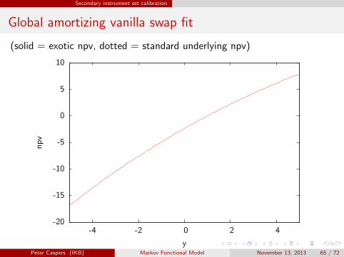
Global amortizing vanilla swap fit
(solid = exotic npv, dotted = standard underlying npv)
-20
-15
-10
-5
0
5
10
-4 -2 0 2 4
np
v
yPeter Caspers (IKB) Markov Functional Model November 13, 2013 65 / 72
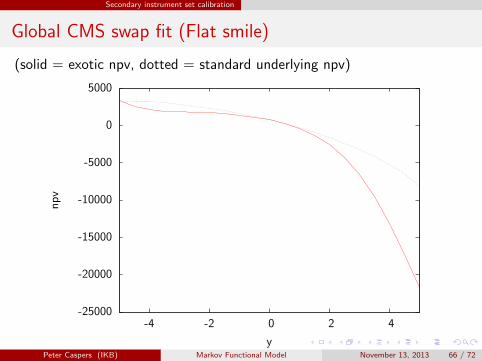
Secondary instrument set calibration
Global CMS swap fit (Flat smile)
(solid = exotic npv, dotted = standard underlying npv)
-25000
-20000
-15000
-10000
-5000
0
5000
-4 -2 0 2 4
np
v
yPeter Caspers (IKB) Markov Functional Model November 13, 2013 66 / 72
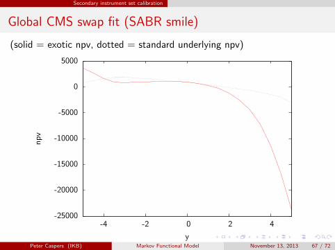
Secondary instrument set calibration
Global CMS swap fit (SABR smile)
(solid = exotic npv, dotted = standard underlying npv)
-25000
-20000
-15000
-10000
-5000
0
5000
-4 -2 0 2 4
np
v
yPeter Caspers (IKB) Markov Functional Model November 13, 2013 67 / 72

Secondary instrument set calibration
Representative Basket Approach - Conclusion
It does not seem to be clear to what secondary instrument set you shouldcalibrate your model in order to represent calls on a cms (or more generallyfloat float) swaps, although in practice atm coterminals seem to be acommon choice.
Peter Caspers (IKB) Markov Functional Model November 13, 2013 68 / 72

Implementation in QuantLib
QuantLib Implementation
A base version of the model is available since release 1.3. Recentdevelopemts (≥ 1.4 ?) include
support for a (zero volatility) spread between discounting andforwarding curves
a float float and non standard swaption pricing engine
representative calibration basket generation
support for pricing under credit risk (credit linked swaptions, exoticbonds)
SABR-Kahale smile preconditioning
Peter Caspers (IKB) Markov Functional Model November 13, 2013 69 / 72

Implementation in QuantLib
Outlook / Future Tasks
Finite Difference pricing engines
Additional smile preconditioning algorithms
Peter Caspers (IKB) Markov Functional Model November 13, 2013 70 / 72
References
References
Johnson, Simon: Numerical methods for the markov functional model,Wilmott magazine, http://www.wilmott.com/pdfs/110802 johnson.pdf
Kahale, Nabil: An arbitrage free interpolation of volatilities, Risk May2004, http://nkahale.free.fr/papers/Interpolation.pdf
Shoup, Victor: NTL A Library for doing Number theory,http://www.shoup.net/ntl/
QuantLib A free/open-source library for quantitative finance,http://www.quantlib.org
Caspers, Peter: Markov Functional One Factor Interest Rate ModelImplementation in QuantLib,http://papers.ssrn.com/sol3/papers.cfm?abstract id=2183721
Caspers, Peter: Representative Basket Method Applied,http://papers.ssrn.com/sol3/papers.cfm?abstract id=2320759
Peter Caspers (IKB) Markov Functional Model November 13, 2013 71 / 72

Questions
Thank you, Questions ?
Peter Caspers (IKB) Markov Functional Model November 13, 2013 72 / 72


![CARB Document: ......CERT STD SFTP @ 4000 miles SFTP @ * miles CO [g/mi] com osite CERT STD CO sc03 CERT 0.09 STD 0.14 CERT 1.7 STD 8.0 CERT 0.04 STD 0.20 CERT 2.4 STD 2.7 CERT STD](https://img.pdfslide.us/doc/110x75/601fc6dcad09a45b411bb1e3/carb-document-cert-std-sftp-4000-miles-sftp-miles-co-gmi-com-osite.jpg)