Markov convexity and local rigidity of distorted metrics

Manor Mendel∗

Open University of Israelmanorme@openu.ac.il

Assaf Naor†

Courant Institutenaor@cims.nyu.edu

Abstract

It is shown that a Banach space admits an equivalent norm whose modulus of uniform con-vexity has power-type p if and only if it is Markov p-convex. Counterexamples are constructed tonatural questions related to isomorphic uniform convexity of metric spaces, showing in particularthat tree metrics fail to have the dichotomy property.

Contents

1 Introduction 21.1 The nonexistence of a metric dichotomy for trees . . . . . . . . . . . . . . . . . . . . 5

1.1.1 Overview of the proofs of Theorem 1.10 and Theorem 1.12 . . . . . . . . . . 7

2 Markov p-convexity and p-convexity coincide 9

3 A doubling space which is not Markov p-convex for any p ∈ (0,∞) 15

4 Lipschitz quotients 17

5 A dichotomy theorem for vertically faithful embeddings of trees 18

6 Tree metrics do not have the dichotomy property 216.1 Horizontally contracted trees . . . . . . . . . . . . . . . . . . . . . . . . . . . . . . . 216.2 Geometry of H-trees . . . . . . . . . . . . . . . . . . . . . . . . . . . . . . . . . . . . 23

6.2.1 Classification of approximate midpoints . . . . . . . . . . . . . . . . . . . . . 236.2.2 Classification of approximate forks . . . . . . . . . . . . . . . . . . . . . . . . 306.2.3 Classification of approximate 3-paths . . . . . . . . . . . . . . . . . . . . . . . 36

6.3 Nonembeddability of vertically faithful B4 . . . . . . . . . . . . . . . . . . . . . . . . 426.4 Nonembeddability of binary trees . . . . . . . . . . . . . . . . . . . . . . . . . . . . . 44

7 Discussion and open problems 45

∗Supported by ISF grant 221/07, BSF grant 2006009, and a gift from Cisco research center.†Supported by NSF grants CCF-0635078 and CCF-0832795, BSF grant 2006009, and the Packard Foundation.

1

1 Introduction

A Banach space (X, ‖ · ‖X) is said to be finitely representable in a Banach space (Y, ‖ · ‖Y ) if thereexists a constant D < ∞ such that for every finite dimensional linear subspace F ⊆ X there is alinear operator T : F → Y satisfying ‖x‖X 6 ‖Tx‖Y 6 D‖x‖X for all x ∈ F . In 1976 Ribe [31]proved that if two Banach spaces X and Y are uniformly homeomorphic, i.e., there is a bijectionf : X → Y such that f and f−1 are uniformly continuous, then X is finitely representable in Yand vice versa. This remarkable theorem motivated what is known today as the “Ribe program”:the search for purely metric reformulations of basic linear concepts and invariants from the localtheory of Banach spaces. This research program was put forth by Bourgain in 1986 [5].

Since its inception, the Ribe program attracted the work of many mathematicians, and led tothe development of several satisfactory metric theories that extend important concepts and resultsof Banach space theory; see the introduction of [24] for a historical discussion. So far, progresson the Ribe program has come hand-in-hand with applications to metric geometry, group theory,functional analysis, and computer science. The present paper contains further progress in thisdirection: we obtain a metric characterization of p-convexity in Banach spaces, derive some ofits metric consequences, and construct unexpected counter-examples which indicate that furtherprogress on the Ribe program can uncover nonlinear phenomena that are markedly different fromtheir Banach space counterparts. In doing so, we answer questions posed by Lee-Naor-Peres andFefferman, and improve a theorem of Bates, Johnson, Lindenstrauss, Preiss and Schechtman. Theseresults, which will be explained in detail below, were announced in [23].

For p > 2, a Banach space (X, ‖ · ‖X) is said to be p-convex if there exists a norm ||| · ||| which isequivalent to ‖ · ‖X (i.e., for some a, b > 0, a‖x‖X 6 |||x||| 6 b‖x‖X for all x ∈ X), and a constantK > 0 satisfying:

|||x||| = |||y||| = 1 =⇒∣∣∣∣∣∣∣∣∣∣∣∣x+ y

2

∣∣∣∣∣∣∣∣∣∣∣∣ 6 1−K|||x− y|||p. (1)

X is called superreflexive if it is p-convex for some p > 2 (historically, this is not the originaldefinition of superreflexivity1, but it is equivalent to it due to a deep theorem of Pisier [29], whichbuilds on important work of James [10] and Enflo [7]). For concreteness, we recall (see, e.g., [2])that Lp is 2-convex for p ∈ (1, 2] and p-convex for p ∈ [2,∞).

Ribe’s theorem implies that p-convexity, and hence also superreflexivity, is preserved underuniform homeomorphisms. The first major success of the Ribe program is a famous theorem ofBourgain [5] which obtains a metrical characterization of superreflexivity as follows.

Theorem 1.1 (Bourgain’s metrical characterization of superreflexivity [5]). Let Bn be the completeunweighted binary tree of depth n, equipped with the natural graph-theoretical metric. Then aBanach space X is superreflexive if and only if

limn→∞

cX(Bn) =∞. (2)

Here, and in what follows, given two metric spaces (M , dM ), (N , dN ), the parameter cM (N )denotes the smallest bi-Lipschitz distortion with which N embeds into M , i.e., the infimum of

1James’ original definition of superreflexivity is that a Banach space X is superreflexive if “its local structure forcesreflexivity”, i.e., if every Banach space Y that is finitely representable in X must be reflexive. Enflo’s renormingtheorem states that superreflexivity is equivalent to having an equivalent norm ||| · ||| that is uniformly convex, i.e.,for every ε ∈ (0, 1) there exists δ > 0 such that if |||x||| = |||y||| = 1 and |||x− y||| = ε then |||x+ y||| 6 2− δ.

2

those D > 0 such that there exists a scaling factor r > 0 and a mapping f : N → M satisfyingrdN (x, y) 6 dM (x, y) 6 DrdN (x, y) for all x, y ∈ N (if no such f exists then set cM (N ) =∞).

Bourgain’s theorem characterizes superreflexivity of Banach spaces in terms of their metricstructure, but it leaves open the characterization of p-convexity. The notion of p-convexity iscrucial for many applications in Banach space theory and metric geometry, and it turns out thatthe completion of the Ribe program for p-convexity requires significant additional work beyondBourgain’s superreflexivity theorem. As a first step in this direction, Lee, Naor and Peres [16]defined a bi-Lipschitz invariant of metric spaces called Markov convexity, which is motivated byBall’s notion of Markov type [1] and Bourgain’s argument in [5].

Definition 1.2 ([16]). Let Xtt∈Z be a Markov chain on a state space Ω. Given an integer k > 0,we denote by Xt(k)t∈Z the process which equals Xt for time t 6 k, and evolves independently(with respect to the same transition probabilities) for time t > k. Fix p > 0. A metric space(X, dX) is called Markov p-convex with constant Π if for every Markov chain Xtt∈Z on a statespace Ω, and every f : Ω→ X,

∞∑k=0

∑t∈Z

E[dX

(f(Xt), f

(Xt

(t− 2k

)))p]2kp

6 Πp ·∑t∈Z

E[dX(f(Xt), f(Xt−1))p

]. (3)

The least constant Π for which (3) holds for all Markov chains is called the Markov p-convexityconstant of X, and is denoted Πp(X). We shall say that (X, dX) is Markov p-convex if Πp(X) <∞.

To gain intuition for Definition 1.2, consider the standard downward random walk starting fromthe root of the binary tree Bn (with absorbing states at the leaves). For an arbitrary mapping ffrom Bn to a metric space (X, dX), the triangle inequality implies that for each k ∈ N we have

∑t∈Z

E[dX

(f(Xt), f

(Xt

(t− 2k

)))p]2kp

.p

∑t∈Z

E[dX(f(Xt), f(Xt−1))p

], (4)

with asymptotic equality (up to constants depending only on p) for k 6 logn2 when X = Bn and f

is the identity mapping. On the other hand, if X is a Markov p-convex space then the sum over k ofthe left-hand side of (4) is uniformly bounded by the right-hand side of (4), and therefore Markovp-convex spaces cannot contain Bn with distortion uniformly bounded in n.

We refer to [16] for more information on the notion of Markov p-convexity. In particular, itis shown in [16] that the Markov 2-convexity constant of an arbitrary weighted tree T is, up toconstant factors, the Euclidean distortion of T . We refer to [16] for Lp versions of this statementand their algorithmic applications. It was also shown in [16], via a modification of an argument ofBourgain [5], that if a Banach space X is p-convex then it is also Markov p-convex. It was askedin [16] if the converse is also true. Here we answer this question positively:

Theorem 1.3. A Banach space is p-convex if and only if it is Markov p-convex.

Thus Markov p-convexity is equivalent to p-convexity in Banach spaces, completing the Ribeprogram in this case. Our proof of Theorem 1.3 is based on a renorming method of Pisier [29]. Itcan be viewed as a nonlinear variant of Pisier’s argument, and several subtle changes are requiredin order to adapt it to a nonlinear condition such as (3).

3

Results similar to Theorem 1.3 have been obtained for the notions of type and cotype of Banachspaces (see [6, 30, 1, 25, 24, 22]), and have been used to transfer some of the linear theory to thesetting of general metric spaces. This led to several applications to problems in metric geometry.Apart from the applications of Markov p-convexity that were obtained in [16], here we show that thisinvariant is preserved under Lipschitz quotients. The notion of Lipschitz quotient was introducedby Gromov [8, Sec. 1.25]. Given two metric spaces (X, dX) and (Y, dY ), a surjective mappingf : X → Y is called a Lipschitz quotient if it is Lipschitz, and it is also “Lipschitzly open” in thesense that there exists a constant c > 0 such that for every x ∈ X and r > 0,

f (BX(x, r)) ⊇ BY(f(x),

r

c

). (5)

Here we show the following result:

Theorem 1.4. If (X, dX) is Markov p-convex and (Y, dY ) is a Lipschitz quotient of X, then Y isalso Markov p-convex.

In [3] Bates, Johnson, Lindenstrauss, Preiss and Schechtman investigated in detail Lipschitzquotients of Banach spaces. Their results imply that if 2 6 p < q then Lq is not a Lipschitzquotient of Lp. Since Lp is p-convex, it is also Markov p-convex. Hence also all of its subsets areMarkov p convex. But, Lq is not p-convex, so we deduce that Lq is not a Lipschitz quotient of anysubset of Lp. Thus our new “invariant approach” to the above result of [3] significantly extends it.Note that the method of [3] is based on a differentiation argument, and hence it crucially relies onthe fact that the Lipschitz quotient mapping is defined on all of Lp and not just on an arbitrarysubset of Lp.

In light of Theorem 1.3 it is natural to ask if Bourgain’s characterization of superreflexivity holdsfor general metric spaces. Namely, is it true that for any metric space X, if limn→∞ cX(Bn) = ∞then X is Markov p-convex for some p <∞? This question was asked in [16], where it was shownthat the answer is positive if (X, dX) is a metric tree. Here we show that in general the answer isnegative:

Theorem 1.5. There exists a metric space (X, dX) which is not Markov p-convex for any p ∈(0,∞), yet limn→∞ cX(Bn) = ∞. In fact, (X, dX) can be a doubling metric space, and hencecX(Bn) > 2κn for some constant κ > 0.

Theorem 1.5 is in sharp contrast to the previously established metric characterizations of thelinear notions of type and cotype. Specifically, it was shown by Bourgain, Milman and Wolfson [6]that any metric space with no nontrivial metric type must contain the Hamming cubes (0, 1n, ‖·‖1)with distortion independent of n. An analogous result was obtained in [24] for metric spaces withno nontrivial metric cotype, with the Hamming cube replaced by the `∞ grid (1, . . . ,mn, ‖ · ‖∞).

Our proof of Theorem 1.5 is based on an analysis of the behavior of a certain Markov chain onthe Laakso graphs: a sequence of combinatorial graphs whose definition is recalled in Section 3. Asa consequence of this analysis, we obtain the following distortion lower bound:

Theorem 1.6. For any p > 2, the Laakso graph of cardinality n incurs distortion Ω((log n)1/p

)in

any embedding into a p-convex Banach space.

Thus, in particular, for p > 2 the n-point Laakso graph incurs distortion Ω((log n)1/p

)in any

embedding into Lp. The case of Lp embeddings of the Laakso graphs when 1 < p 6 2 was already

4

solved in [26, 12, 15, 14] using the uniform 2-convexity property of Lp. But, these proofs relycrucially on 2-convexity and do not extend to the case of p-convexity when p > 2. Subsequent tothe publication of our proof of Theorem 1.6 in the announcement [23], an alternative proof of thisfact was recently discovered by Johnson and Schechtman in [11].

1.1 The nonexistence of a metric dichotomy for trees

Bourgain’s metrical characterization of superreflexivity yields the following statement:

Theorem 1.7 (Bourgain’s tree dichotomy [5]). For any Banach space (X, ‖·‖X) one of the followingtwo dichotomic possibilities must hold true:

• either for all n ∈ N we have cX(Bn) = 1,

• or there exists α = αX > 0 such that for all n ∈ N we have cX(Bn) > (log n)α.

Thus, there is a gap in the possible rates of growth of the sequence cX(Bn)∞n=1 when X isa Banach space; consequently, if we were told that, say, cX(Bn) = O(log log n), then we wouldimmediately deduce that actually cX(Bn) = 1 for all n. Additional gap results of this type areknown due to the theory of nonlinear type and cotype:

Theorem 1.8 (Bourgain-Milman-Wolfson cube dichotomy [6]). For any metric space (X, dX) oneof the following two dichotomic possibilities must hold true:

• either for all n ∈ N we have cX (0, 1n, ‖ · ‖1) = 1,

• or there exists α = αX > 0 such that for all n ∈ N we have cX (0, 1n, ‖ · ‖1) > nα.

Theorem 1.8 is a metric analogue of Pisier’s characterization [28] of Banach spaces with trivialRademacher type. A metric analogue of the Maurey-Pisier characterization [20] of Banach spaceswith finite Rademacher cotype yields the following dichotomy result for `∞ grids:

Theorem 1.9 (Grid dichotomy [24]). For any metric space (X, dX) one of the following twodichotomic possibilities must hold true:

• either for all n ∈ N we have cX (0, . . . , nn, ‖ · ‖∞) = 1,

• or there exists α = αX > 0 such that for all n ∈ N we have cX (0, . . . , nn, ‖ · ‖∞) > nα.

We refer to the survey article [21] for more information on the theory of metric dichotomies.Note that Theorem 1.7 is stated for Banach spaces, while Theorem 1.8 and Theorem 1.9 hold

for general metric spaces. One might expect that as in the case of previous progress on Ribe’sprogram, a metric theory of p-convexity would result in a proof that Theorem 1.7 holds when X isa general metric space. Surprisingly, we show here that this is not true:

Theorem 1.10. There exists a universal constant C > 0 with the following property. Assume thats(n)∞n=0 ⊆ [4,∞) is a nondecreasing sequence such that n/s(n)∞n=0 is also nondecreasing. Thenthere exists a metric space (X, dX) satisfying for all n > 2,

s

(⌊n

40s(n)

⌋)(1− Cs(n) log s(n)

log n

)6 cX(Bn) 6 s(n). (6)

5

Thus, assuming that s(n) = o(

lognlog logn

), there exists a subsequence nk∞k=1 for which

(1− o(1))s(nk) 6 cX(Bnk) 6 s(nk). (7)

Theorem 1.10 shows that unlike the case of Banach spaces, for general metric spaces, cX(Bn)can have an arbitrarily slow growth rate.

Bourgain, Milman and Wolfson also obtained in [6] the following finitary version of Theorem 1.8:

Theorem 1.11 (Local rigidity of Hamming cubes [6]). For every ε > 0, D > 1 and n ∈ N thereexists m = m(ε,D, n) ∈ N such that

limn→∞

m(ε,D, n) =∞,

and for every metric d on 0, 1n which is bi-Lipschitz with distortion 6 D to the `1 (Hamming)metric,

c(0,1n,d) (0, 1m, ‖ · ‖1) 6 1 + ε.

We refer to [6] (see also [30]) for bounds on m(ε,D, n). Informally, Theorem 1.11 says that theHamming cube (0, 1n, ‖ · ‖1) is locally rigid in the following sense: it is impossible to distort theHamming metric on a sufficiently large hypercube without the resulting metric space containinga hardly distorted copy of an arbitrarily large Hamming cube. Stated in this way, Theorem 1.11is a metric version of James’ theorem [9] that `1 is not a distortable space. The analogue ofTheorem 1.11 with the Hamming cube replaced by the `∞ grid (0, . . . , nn, ‖ · ‖∞) is Matousek’sBD-Ramsey theorem [19]; see [24] for quantitative results of this type in the `∞ case. The followingvariant of Theorem 1.10 shows that a local rigidity statement as above fails to hold true for binarytrees; it can also be viewed as a negative solution of the distortion problem for the infinite binarytree (see [27] and [4, Ch. 13, 14] for more information on the distortion problem for Banach spaces).

Theorem 1.12. Let B∞ be the complete unweighted infinite binary tree. For every D > 4 thereexists a metric d on B∞ that is D-equivalent to the original shortest-path metric on B∞, yet forevery ε ∈ (0, 1) and m ∈ N,

c(B∞,d)(Bm) 6 D − ε =⇒ m 6 DCD2/ε.

The local rigidity problem for binary trees was studied by several mathematicians. In partic-ular, C. Fefferman asked (private communication, 2005) whether Bn∞n=1 have the local rigidityproperty, and Theorem 1.12 answers this question negatively. Fefferman also proved a partial localrigidity result which is a non-quantitative variant of Theorem 1.14 below (see also Section 5). Weare very grateful to C. Fefferman for asking us the question that led to the counter-examples ofTheorem 1.10 and Theorem 1.12, for sharing with us his partial positive results, and for encouragingus to work on these questions. M. Gromov also investigated the local rigidity problem for binarytrees, and proved (via different methods) non-quantitative partial positive results in the spirit ofTheorem 1.14. We thank M. Gromov for sharing with us his unpublished work on this topic.

The results of Theorem 1.10 and Theorem 1.12 are quite unexpected. Unfortunately, their proofsare delicate and lengthy, and as such constitute the most involved part of this article. In order tofacilitate the understanding of these constructions, we end the introduction with an overview ofthe main geometric ideas that are used in their proofs. This is done in Section 1.1.1 below—werecommend reading this section first before delving into the technical details presented in Section 6.

6

1.1.1 Overview of the proofs of Theorem 1.10 and Theorem 1.12

For x ∈ B∞ let h(x) be its depth, i.e., its distance from the root. Also, for x, y ∈ B∞ let lca(x, y)denote their least common ancestor. The tree metric on B∞ is then given by:

dB∞(x, y) = h(x) + h(y)− 2h(lca(x, y)).

The metric space X of Theorem 1.10 will be B∞ as a set, with a new metric defined as follows.Given a sequence ε = εn∞n=0 ⊆ (0, 1] we define dε : B∞ ×B∞ → [0,∞) by

dε(x, y) = |h(y)− h(x)|+ 2εminh(x),h(y) · [minh(x), h(y) − h(lca(x, y))] .

dε does not necessarily satisfy the triangle inequality, but under some simple conditions on thesequence εn∞n=0 it does become a metric on B∞; see Lemma 6.1. A pictorial description of themetric dε is contained in Figure 1. Note that when εn = 1 for all n, we have dε = dB∞ . Below wecall the metric spaces (B∞, dε) horizontally distorted trees, or H-trees, in short.

lca(x, y)

x

y

b

a

root

dε(x, y) = b + 2a · εh(x)

Figure 1: The metric dε defined on B∞. The arrows indicate horizontal contraction by εh(x).

The metric space (X, dX) of Theorem 1.10 will be (B∞, dε), where εn = 1/s(n) for all n. Theidentity mapping of Bn into the top n-levels of B∞ has distortion at most s(n), and thereforecX(Bn) 6 s(n). The challenge is to prove the lower bound on cX(Bn) in (6). Our initial approachto lower-bounding cX(Bn) was Matousek’s metric differentiation proof [18] of asymptotically sharpdistortion lower bounds for embeddings of Bn into uniformly convex Banach spaces.

Following Matousek’s terminology [18], for δ > 0 a quadruple of points (x, y, z, w) in a met-ric space (X, dX) is called a δ-fork if y ∈ Mid(x, z, δ) ∩ Mid(x,w, δ), where for a, b ∈ X theset of δ-approximate midpoints Mid(a, b, δ) ⊆ X is defined as the set of all w ∈ X satisfyingmaxdX(x, y), dX(y, z) 6 1+δ

2 · dX(x, z). The points z, w will be called below the prongs of theδ-fork (x, y, z, w). Matousek starts with the observation that if X is a uniformly convex Banachspace then in any δ-fork in X the distance between the prongs must be much smaller (as δ → 0)than dX(x, y). Matousek then shows that for all D > 0, any distortion D embedding of Bn into Xmust map some 0-fork in Bn to a δ-fork in X, provided n is large enough (as a function of D andδ). This reasoning immediately implies that cX(Bn) must be large when X is a uniformly convexBanach space, and a clever argument of Matousek in [18] turns this qualitative argument into sharpquantitative bounds.

7

Of course, we cannot hope to use the above argument of Matousek in order to prove Theo-rem 1.10, since Bourgain’s tree dichotomy theorem (Theorem 1.7) does hold true for Banach spaces.But, perhaps we can mimic this uniform convexity argument for other target metric spaces? Onthe face of it, H-trees are ideally suited for this purpose, since the horizontal contractions that weintroduced shrink distances between the prongs of canonical forks (call (x, y, z, w) ∈ B∞ a canonicalfork if x is an ancestor of y and z, w are descendants of y at depth h(x) + 2(h(y)− h(x))). It is forthis reason exactly that we defined H-trees.

Unfortunately, the situation isn’t so simple. It turns out that H-trees do not behave likeuniformly convex Banach spaces in terms of the prong-contractions that they impose of δ-forks.H-trees can even contain larger problematic configurations that have several undistorted δ-forks;such an example is depicted in Figure 2.

r

h2 − h1 = δ−1

h1

h2

r

Figure 2: The metric space on the right is the H-tree (B∞, dε), where εn = δ for all n. The picturedescribes an embedding of the tree on the left (B3 minus 4 leaves) into (B∞, dε) with distortion atmost 6, yet all ancestor/descendant distances are distorted by at most 1 +O(δ).

Thus, in order to prove Theorem 1.10 it does not suffice to use Matousek’s argument that abi-Lipschitz embedding of a large enough Bn must send some 0-fork to a δ-fork. But, it turns outthat this argument applies not only to forks, but also to larger configurations.

Definition 1.13. Let (T, dT ) be a tree with root r, and let (X, dX) be a metric space. A mappingf : T → X is called a D-vertically faithful embedding if there exists a (scaling factor) λ > 0satisfying for any x, y ∈ T such that x is an ancestor of y,

λdT (x, y) 6 dX(f(x), f(y)) 6 DλdT (x, y). (8)

Recall that the distortion of a mapping φ : M → N between metric spaces (M , dM ) and(N , dN ) is defined as

dist(φ)def=

supx,y∈Mx 6=y

dN (φ(x), φ(y))

dM (x, y)

· supx,y∈Mx 6=y

dM (x, y)

dN (φ(x), φ(y))

∈ [1,∞].

With this terminology, we can state the following crucial result.

8

Theorem 1.14. There exists a universal constant c > 0 with the following property. Fix an integert > 2, δ, ξ ∈ (0, 1), and D > 2, and assume that n ∈ N satisfies

n >1

ξDc(t log t)/δ. (9)

Let (X, dX) be a metric space and f : Bn → X a D-vertically faithful embedding. Then there existsa mapping φ : Bt → Bn with the following properties.

• If x, y ∈ Bt are such that x is an ancestor of y, then φ(x) is an ancestor of φ(y).

• dist(φ) 6 1 + ξ.

• The mapping f φ : Bt → X is a (1 + δ)-vertically faithful embedding of Bt in X.

Theorem 1.14 is essentially due to Matousek [18]. Matousek actually proved this statementonly for t = 2, since this is all that he needed in order to analyze forks. But, his proof extends ina straightforward way to any t ∈ N. Since we will use this assertion with larger t, for the sake ofcompleteness we reprove it, in a somewhat different way, in Section 5. Note that Theorem 1.14 saysthat Bn∞n=1 do have a local rigidity property with respect to vertically faithfully embeddings.

We solve the problem created by the existence of configurations as those depicted in Figure 2 bystudying (1 + δ)-vertically faithful embeddings of B4, and arguing that they must contain a largecontracted pair of points. This claim, formalized in Lemma 6.27, is proved in Sections 6.2, 6.3.

We begin in Section 6.2.1 with studying how the metric P2 (3-point path) can be approximatelyembedded in (B∞, dε). We find that there are essentially only two ways to embed it in (B∞, dε),as depicted in Figure 3. We then proceed in Section 6.2.2 to study δ-forks in (B∞, dε). Sinceforks are formed by “stitching” two approximate P2 metrics along a common edge (the handle), wecan limit the “search space” using the results of Section 6.2.1. We find that there are six possibletypes of different approximate forks in (B∞, dε), only four of which (depicted in Figure 4) do nothave highly contracted prongs. Complete binary trees, and in particular B4, are composed of forksstitched together, handle to prong. In order to study handle-to-prong stitching, we investigate inSection 6.2.3 how the metric P3 (4-point path) can be approximately embedded in (B∞, dε). Thisis again done by studying how two P2 metrics can be stitched together, this time bottom edge totop edge. We find that there are only three different approximate configurations of P4 in (B∞, dε).

Using the machinery described above, we study in Section 6.3 how the different types of forkscan be stitched together in embeddings of B4 into (B∞, dε), reaching the conclusion that a large con-traction is unavoidable, and thus completing the proof of Lemma 6.27. The proofs of Theorem 1.10and Theorem 1.12 are concluded in Section 6.4.

2 Markov p-convexity and p-convexity coincide

In this section we prove Theorem 1.3, i.e., that for Banach spaces p-convexity and Markov p-convexity are the same properties. We first show that p-convexity implies Markov p-convexity,and in fact it implies a stronger inequality that is stated in Proposition 2.1 below. The slightlyweaker assertion that p-convexity implies Markov p-convexity was first proved in [16], based on anargument from [5]. Our argument here is different and simpler.

9

It was proved in [29] that a Banach space X is p-convex if and only if it admits an equivalentnorm ‖ · ‖ for which there exists K > 0 such that for every a, b ∈ X,

2‖a‖p +2

Kp‖b‖p 6 ‖a+ b‖p + ‖a− b‖p. (10)

Proposition 2.1. Let Xtt∈Z be random variables taking values in a set Ω. For every s ∈ Z letXt(s)

t∈Z

be random variables taking values in Ω, with the following property:

∀ r 6 s 6 t, (Xr, Xt) and(Xr, Xt(s)

)have the same distribution. (11)

Fix p > 2 and let (X, ‖ ·‖) be a Banach space whose norm satisfies (10). Then for every f : Ω→ Xwe have

∞∑k=0

∑t∈Z

E[∥∥∥f(Xt)− f

(Xt(t− 2k)

)∥∥∥p]2kp

6 (4K)p∑t∈Z

E[‖f(Xt)− f(Xt−1)‖p

]. (12)

Remark 2.2. Observe that condition (11) holds when Xtt∈Z is a Markov chain on a state space

Ω, andXt(s)

t∈Z

is as in Definition 1.2.

We start by proving a useful inequality that is a simple consequence of (10).

Lemma 2.3. Let X be a Banach space whose norm satisfies (10). Then for every x, y, z, w ∈ X,

‖x− w‖p + ‖x− z‖p2p−1

+‖z − w‖p4p−1Kp

6 ‖y − w‖p + ‖z − y‖p + 2‖y − x‖p. (13)

Proof. For every x, y, z, w ∈ X, (10) implies that

‖x− w‖p2p−1

+2

Kp

∥∥∥∥y − x+ w

2

∥∥∥∥p 6 ‖y − x‖p + ‖y − w‖p,

and‖z − x‖p

2p−1+

2

Kp

∥∥∥∥y − z + x

2

∥∥∥∥p 6 ‖z − y‖p + ‖y − x‖p.

Summing these two inequalities, and applying the convexity of the map u 7→ ‖u‖p, we see that

‖y − w‖p + ‖z − y‖p + 2‖y − x‖p > ‖x− w‖p + ‖z − x‖p2p−1

+4

Kp·∥∥y − x+w

2

∥∥p +∥∥y − z+x

2

∥∥p2

>‖x− w‖p + ‖z − x‖p

2p−1+

4

Kp·∥∥∥∥z − w4

∥∥∥∥p ,implying (13).

Proof of Proposition 2.1. Using Lemma 2.3 we see that for every t ∈ Z and k ∈ N,

‖f(Xt)− f(Xt−2k)‖p + ‖f(Xt(t− 2k−1))− f(Xt−2k)‖p2p−1

+‖f(Xt)− f(Xt(t− 2k−1))‖p

4p−1Kp

6 ‖f(Xt−2k−1)− f(Xt)‖p + ‖f(Xt−2k−1)− f(Xt(t− 2k−1))‖p + 2‖f(Xt−2k−1)− f(Xt−2k)‖p.

10

Taking expectation, and using the assumption (11), we get

E[‖f(Xt)− f(Xt−2k)‖p

]2p−2

+E[‖f(Xt)− f(Xt(t− 2k−1))‖p

]4p−1Kp

6 2E[‖f(Xt−2k−1)− f(Xt)‖p

]+ 2E

[‖f(Xt−2k−1)− f(Xt−2k)‖p

].

Dividing by 2(k−1)p+2 this becomes

E[‖f(Xt)− f(Xt−2k)‖p

]2kp

+E[‖f(Xt)− f(Xt(t− 2k−1))‖p

]2(k+1)pKp

6E[‖f(Xt−2k−1)− f(Xt)‖p

]2(k−1)p+1

+E[‖f(Xt−2k−1)− f(Xt−2k)‖p

]2(k−1)p+1

.

Summing this inequality over k = 1, . . . ,m and t ∈ Z we get

m∑k=1

∑t∈Z

E[‖f(Xt)− f(Xt−2k)‖p

]2kp

+

m∑k=1

∑t∈Z

[E‖f(Xt)− f(Xt(t− 2k−1))‖p

]2(k+1)pKp

6m∑k=1

∑t∈Z

E[‖f(Xt−2k−1)− f(Xt)‖p

]2(k−1)p+1

+

m∑k=1

∑t∈Z

E[‖f(Xt−2k−1)− f(Xt−2k)‖p

]2(k−1)p+1

=m−1∑j=0

∑s∈Z

E [‖f(Xs)− f(Xs−2j )‖p]2jp

. (14)

It is only of interest to prove (12) when∑

t∈Z E[‖f(Xt) − f(Xt−1)‖p

]< ∞. By the triangle

inequality, this implies that for every k ∈ N we have∑

t∈Z E[‖f(Xt)− f(Xt−2k)‖p

]<∞. We may

therefore cancel terms in (14), arriving at the following inequality:

m∑k=1

∑t∈Z

E[‖f(Xt)− f(Xt(t− 2k−1))‖p

]2(k+1)pKp

6∑t∈Z

E [‖f(Xt)− f(Xt−1)‖p]−∑t∈Z

E [‖f(Xt)− f(Xt−2m)‖p]2mp

6∑t∈Z

E [‖f(Xt)− f(Xt−1)‖p] .

Equivalently,

m−1∑k=0

∑t∈Z

E[‖f(Xt)− f(Xt(t− 2k))‖p

]2kp

6 (4K)p∑t∈Z

E [‖f(Xt)− f(Xt−1)‖p] .

Proposition 2.1 now follows by letting m→∞.

We next prove the more interesting direction of the equivalence of p-convexity and Markovp-convexity: a Markov p-convex Banach space is also p-convex.

11

Theorem 2.4. Let (X, ‖ · ‖) be a Banach space which is Markov p-convex with constant Π. Thenfor every ε ∈ (0, 1) there exists a norm ||| · ||| on X such that for all x, y ∈ X,

(1− ε)‖x‖ 6 |||x||| 6 ‖x‖,

and ∣∣∣∣∣∣∣∣∣∣∣∣x+ y

2

∣∣∣∣∣∣∣∣∣∣∣∣p 6 |||x|||p + |||y|||p2

− 1− (1− ε)p4Πp(p+ 1)

·∣∣∣∣∣∣∣∣∣∣∣∣x− y2

∣∣∣∣∣∣∣∣∣∣∣∣p .Thus the norm ||| · ||| satisfies (10) with constant K = O

(Πε1/p

).

Proof. The fact that X is Markov p-convex with constant Π implies that for every Markov chainXtt∈Z with values in X, and for every m ∈ N, we have

m∑k=0

2m∑t=1

E[∥∥Xt − Xt(t− 2k)

∥∥p]2kp

6 Πp2m∑t=1

E [‖Xt −Xt−1‖p] . (15)

For x ∈ X we shall say that a Markov chain Xt2mt=−∞ is an m-admissible representation of xif Xt = 0 for t 6 0 and E [Xt] = tx for t ∈ 1, . . . , 2m. Fix ε ∈ (0, 1), and denote η = 1− (1− ε)p.For every m ∈ N define

|||x|||m = inf

1

2m

2m∑t=1

E [‖Xt −Xt−1‖p]−η

Πp· 1

2m

m∑k=0

2m∑t=1

E[∥∥Xt − Xt(t− 2k)

∥∥p]2kp

1/p , (16)

where the infimum in (16) is taken over all m-admissible representations of x. Observe that anm-admissible representation of x always exists, since we can define Xt = 0 for t 6 0 and Xt = txfor t ∈ 1, . . . , 2m. This example shows that |||x|||m 6 ‖x‖. On the other hand, if Xt2mt=−∞ is anm-admissible representation of x then

2m∑t=1

E [‖Xt −Xt−1‖p]−η

Πp

m∑k=0

2m∑t=1

E[∥∥Xt − Xt(t− 2k)

∥∥p]2kp

(15)

> (1− η)2m∑t=1

E [‖Xt −Xt−1‖p]

> (1− ε)p2m∑t=1

‖E [Xt]− E [Xt−1]‖p = (1− ε)p2m∑t=1

‖tx− (t− 1)x‖p = 2m(1− ε)p‖x‖p, (17)

where in the first inequality of (17) we used the convexity of the function z 7→ ‖z‖p. In conclusion,we see that for all x ∈ X,

(1− ε)‖x‖ 6 |||x|||m 6 ‖x‖. (18)

Now take x, y ∈ X and fix δ ∈ (0, 1). Let Xt2mt=−∞ be an admissible representation on x andYt2mt=−∞ be an admissible representation of y which is stochastically independent of Xt2mt=−∞,such that

2m∑t=1

E [‖Xt −Xt−1‖p]−η

Πp

m∑k=0

2m∑t=1

E[∥∥Xt − Xt(t− 2k)

∥∥p]2kp

6 2m(|||x|||pm + δ), (19)

12

and2m∑t=1

E [‖Yt − Yt−1‖p]−η

Πp

m∑k=0

2m∑t=1

E[∥∥Yt − Yt(t− 2k)

∥∥p]2kp

6 2m(|||y|||pm + δ). (20)

Define a Markov chain Zt2m+1

t=−∞ ⊆ X as follows. For t 6 −2m set Zt = 0. With probability 12

let (Z−2m+1, Z−2m+2, . . . , Z2m+1) equal(0, . . . , 0︸ ︷︷ ︸2m times

, X1, X2, . . . , X2m , X2m + Y1, X2m + Y2, . . . , X2m + Y2m

),

and with probability 12 let (Z−2m+1, Z−2m , . . . , Z2m+1) equal(

0, . . . , 0︸ ︷︷ ︸2m times

, Y1, Y2, . . . , Y2m , X1 + Y2m , X2 + Y2m , . . . , X2m + Y2m

).

Hence, Zt = 0 for t 6 0, for t ∈ 1, . . . , 2m we have E [Zt] = E[Xt]+E[Yt]2 = t · x+y

2 , and fort ∈ 2m + 1, . . . , 2m+1 we have

E [Zt] =E [X2m + Yt−2m ] + E [Xt−2m + Y2m ]

2=

2mx+ (t− 2m)y + (t− 2m)x+ 2my

2= t · x+ y

2.

Thus Zt2m+1

t=−∞ is an (m+1)-admissible representation of x+y2 . The definition (16) implies that

2m+1

∣∣∣∣∣∣∣∣∣∣∣∣x+ y

2

∣∣∣∣∣∣∣∣∣∣∣∣pm+1

62m+1∑t=1

E [‖Zt − Zt−1‖p]−η

Πp

m+1∑k=0

2m+1∑t=1

E[∥∥Zt − Zt(t− 2k)

∥∥p]2kp

. (21)

Note that by definition,

2m+1∑t=1

E [‖Zt − Zt−1‖p] =2m∑t=1

E [‖Xt −Xt−1‖p] +2m∑t=1

E [‖Yt − Yt−1‖p] . (22)

Moreover,

m+1∑k=0

2m+1∑t=1

E[∥∥Zt − Zt(t− 2k)

∥∥p]2kp

=1

2(m+1)p

2m+1∑t=1

E[∥∥Zt − Zt(t− 2m+1)

∥∥p]+

m∑k=0

2m+1∑t=1

E[∥∥Zt − Zt(t− 2k)

∥∥p]2kp

. (23)

We bound each of the terms in (23) separately. Note that by construction we have for everyt ∈ 1, . . . , 2m,

Zt − Zt(t− 2m+1

)= Zt − Zt

(1− 2m+1

)=

Xt − Yt with probability 1/4,

Yt −Xt with probability 1/4,

Xt − Xt(1) with probability 1/4,

Yt − Yt(1) with probability 1/4.

13

Thus, the first term in the right hand side of (23) can be bounded from below as follows:

1

2(m+1)p

2m+1∑t=1

E[∥∥Zt − Zt(t− 2m+1)

∥∥p] > 1

2(m+1)p+1

2m∑t=1

E [‖Xt − Yt‖p]

>1

2(m+1)p+1

2m∑t=1

‖E [Xt]− E [Yt] ‖p =‖x− y‖p2(m+1)p+1

2m∑t=1

tp >2m‖x− y‖p2p+1(p+ 1)

. (24)

We now proceed to bound from below the second term in the right hand side of (23). Note firstthat for every k ∈ 0, . . . ,m and every t ∈ 2m + 1, . . . , 2m+1 we have

Zt−Zt(t−2k) =

(X2m + Yt−2m)−(X2m(t− 2k) + Yt−2m(t− 2m − 2k)

)with probability 1/2,

(Y2m +Xt−2m)−(Y2m(t− 2k) + Xt−2m(t− 2m − 2k)

)with probability 1/2.

By Jensen’s inequality, if U, V are X-valued independent random variables with E[V ] = 0, thenE [‖U + V ‖p] > E [‖U + E[V ]‖p] = E [‖U‖p]. Thus, since Xt2mt=−∞ and Yt2mt=−∞ are independent,

E[∥∥Yt−2m − Yt−2m(t− 2m − 2k) +X2m − X2m(t− 2k)

∥∥p]> E

[∥∥Yt−2m − Yt−2m(t− 2m − 2k)∥∥p] ,

and

E[∥∥Xt−2m − Xt−2m(t− 2m − 2k) + Y2m − Y2m(t− 2k)

∥∥p]> E

[∥∥Xt−2m − Xt−2m(t− 2m − 2k)∥∥p] .

It follows that for every k ∈ 0, . . . ,m and every t ∈ 2m + 1, . . . , 2m+1 we have

E[∥∥Zt − Zt(t− 2k)

∥∥p]>

1

2E[∥∥Xt−2m − Xt−2m(t− 2m − 2k)

∥∥p]+1

2E[∥∥Yt−2m − Yt−2m(t− 2m − 2k)

∥∥p] . (25)

Hence,

m∑k=0

2m+1∑t=1

E[∥∥Zt − Zt(t− 2k)

∥∥p]2kp

(25)

>m∑k=0

2m∑t=1

12E[∥∥Xt − Xt(t− 2k)

∥∥p]+ 12E[∥∥Yt − Yt(t− 2k)

∥∥p]2kp

+m∑k=0

2m+1∑t=2m+1

12

[E∥∥Xt−2m − Xt−2m(t− 2m − 2k)

∥∥p]+ 12E[∥∥Yt−2m − Yt−2m(t− 2m − 2k)

∥∥p]2kp

=m∑k=0

2m∑t=1

E[∥∥Xt − Xt(t− 2k)

∥∥p]2kp

+m∑k=0

2m∑t=1

E[∥∥Yt − Yt(t− 2k)

∥∥p]2kp

. (26)

Combining (19), (20), (21), (22), (23), (24) and (26), and letting δ tend to 0, we see that

2m+1

∣∣∣∣∣∣∣∣∣∣∣∣x+ y

2

∣∣∣∣∣∣∣∣∣∣∣∣pm+1

6 2m|||x|||pm + 2m|||y|||pm −η

Πp· 2m‖x− y‖p

2p+1(p+ 1),

14

or, ∣∣∣∣∣∣∣∣∣∣∣∣x+ y

2

∣∣∣∣∣∣∣∣∣∣∣∣pm+1

6|||x|||pm + |||y|||pm

2− η

4Πp(p+ 1)·∥∥∥∥x− y2

∥∥∥∥p . (27)

Define for w ∈ X,|||w||| = lim sup

m→∞|||w|||m.

Then a combination of (18) and (27) yields that

(1− ε)‖x‖ 6 |||x||| 6 ‖x‖,

and∣∣∣∣∣∣∣∣∣∣∣∣x+ y

2

∣∣∣∣∣∣∣∣∣∣∣∣p 6 |||x|||p + |||y|||p2

− η

4Πp(p+ 1)·∥∥∥∥x− y2

∥∥∥∥p6|||x|||p + |||y|||p

2− η

4Πp(p+ 1)·∣∣∣∣∣∣∣∣∣∣∣∣x− y2

∣∣∣∣∣∣∣∣∣∣∣∣p . (28)

Note that (28) implies that the set x ∈ X : |||x||| 6 1 is convex, so that ||| · ||| is a norm on X.This concludes the proof of Theorem 2.4.

3 A doubling space which is not Markov p-convex for any p ∈ (0,∞)

G1

G0

G2

G3

r

r

r

r

b

Consider the Laakso graphs [12], Gi∞i=0, which aredefined as follows. G0 is the graph consisting of one edgeof unit length. To construct Gi, take six copies of Gi−1

and scale their metric by a factor of 14 . We glue four of

them cyclicly by identifying pairs of endpoints, and attachat two opposite gluing points the remaining two copies.Note that each edge of Gi has length 4−i; we denoted theresulting shortest path metric on Gi by dGi . As shownin [13, Thm. 2.3], the doubling constant of metric space(Gi, dGi) is at most 6.

We direct Gm as follows. Define the root of Gm to be(an arbitrarily chosen) one of the two vertices having onlyone adjacent edge. In the figure this could be the leftmostvertex r. Note that in no edge the two endpoints are at the same distance from the root. Theedges of Gm are then directed from the endpoint closer to the root to the endpoint further awayfrom the root. The resulting directed graph is acyclic. We now define Xt4mt=0 to be the standardrandom walk on the directed graph Gm, starting from the root. This random walk is extended tot ∈ Z by stipulating that Xt = X0 for t < 0, and Xt = X4m for t > 4m.

Proposition 3.1. For the random walk defined above,

2m∑k=0

∑t∈Z

E[dGm

(Xt, Xt(t− 2k)

)p]2kp

&m

8p

∑t∈Z

E [dGm(Xt, Xt−1)p] . (29)

15

Proof. For every t ∈ Z we have,

E [dGm(Xt, Xt−1)p] =

4−mp t ∈ 0, . . . 4m − 1,0 otherwise.

Hence, ∑t∈Z

E [dGm(Xt, Xt−1)p] = 4−m(p−1). (30)

Fix k ∈ 0, . . . , 2m− 2 and write h = dk/2e. View Gm as being built from A = Gm−h, whereeach edge of A has been replaced by a copy of Gh. Note that for every i ∈ 0, . . . , 4m−h−1 + 1, attime t = (4i+ 1)4h the walk Xt is at a vertex of Gm which has two outgoing edges, correspondingto distinct copies of Gh. To see this it suffices to show that all vertices of Gm−h that are exactly(4i+ 1) edges away from the root, have out-degree 2. This fact is true since Gm−h is obtained fromGm−h−1 by replacing each edge by a copy of G1, and each such copy of G1 contributes one vertexof out-degree 2, corresponding to the vertex labeled b in the figure describing G1.

Consider the set of times

Tkdef= 0, . . . , 4m − 1

⋂4m−h−1+1⋃i=0

[(4i+ 1)4h + 4h−2, (4i+ 1)4h + 2 · 4h−2

] .

For t ∈ Tk find i ∈ 0, . . . , 4m−h−1 + 1 such that t ∈[(4i + 1)4h + 4h−2, (4i + 1)4h + 2 · 4h−2

].

Since, by the definition of h, we have t − 2k ∈[(4i + 1)4h − 4h, (4i + 1)4h

), the walks Xss∈Z

and Xs(t− 2k)s∈Z started evolving independently at some vertex lying in a copy of Gh precedinga vertex v of Gm which has two outgoing edges, corresponding to distinct copies of Gh. Thus,with probability at least 1

2 , the walks Xt and Xt(t − 2k) lie on two distinct copies of Gh in Gm,immediately following the vertex v, and at distance at least 4h−2 ·4−m and at most 2·4h−2 ·4−m from

v. Hence, with probability at least 12 we have dGm

(Xt, Xt(t− 2k)

)> 2 · 4h−2 · 4−m = 22h−3−2m,

and therefore,

E[d(Xt, Xt(t− 2k))p

]2kp

>122(2h−3−2m)p

2kp> 2−(2m+3)p−1.

We deduce that for all k ∈ 0, . . . , 2m− 2,

∑t∈Z

E[d(Xt, Xt(t− 2k))p

]2kp

>∑t∈Tk

E[d(Xt, Xt(t− 2k))p

]2kp

> |Tk| · 2−(2m+3)p−1

& 4h−2 · 4m−h−1 · 2−(2m+3)p−1 &1

8p4−m(p−1). (31)

A combination of (30) and (31) implies (29).

Proof of Theorem 1.5. As explained in [12, 13], by passing to an appropriate Gromov-Hausdorfflimit, there exists a doubling metric space (X, dX) that contains an isometric copy of all theLaakso graphs Gm∞m=0. Proposition 3.1 therefore implies that X is not Markov p-convex for anyp ∈ (0,∞).

16

Proof of Theorem 1.6. Let (X, dX) be a Markov p-convex metric space, i.e, Πp(X) < ∞. Assumethat f : Gm → X satisfies

x, y ∈ Gm =⇒ 1

AdGm(x, y) 6 dX(f(x), f(y)) 6 BdGm(x, y). (32)

Let Xtt∈Z be the random walk from Proposition 3.1. Then

m

8pAp

∑t∈Z

E [dGm(Xt, Xt−1)p](29)

.1

Ap

2m∑k=0

∑t∈Z

E[dGm

(Xt, Xt(t− 2k)

)p]2kp

(32)

62m∑k=0

∑t∈Z

E[dX(f(Xt), f(Xt(t− 2k))

)p]2kp

(3)

6 Πp(X)p∑t∈Z

E [dX(f(Xt), f(Xt−1))p]

(32)

6 Πp(X)pBp∑t∈Z

E [dGm(Xt, Xt−1)p] .

Thus AB & m1/p & (log |Gm|)1/p.

4 Lipschitz quotients

Say that a metric space (Y, dY ) is a D-Lipschitz quotient of a metric space (X, dX) if there exista, b > 0 with ab 6 D and a mapping f : X → Y such that for all x ∈ X and r > 0,

BY

(f(x),

r

a

)⊆ f (BX(x, r)) ⊆ BY (f(x), br). (33)

Observe that the last inclusion in (33) is to equivalent to the fact that f is b-Lipschitz.The following proposition implies Theorem 1.4.

Proposition 4.1. If (Y,DY ) is a D-Lipschitz quotient of (X, dX) then Πp(Y ) 6 D ·Πp(X).

Proof. Fix f : X → Y satisfying (33). Also, fix a Markov chain Xtt∈Z on a state space Ω, and amapping g : Ω→ Y .

Fix m ∈ Z and let Ω∗ be the set of finite sequences of elements of Ω starting at time m, i.e.,the set of sequences of the form (ωi)

ti=m ∈ Ωt−m+1 for all t > m. It will be convenient to consider

the Markov chain X∗t ∞t=m on Ω∗ which is given by:

Pr [X∗t = (ωm, ωm+1, . . . , ωt)] = Pr [Xm = ωm, Xm+1 = ωm+1, . . . , Xt = ωt] .

Also, define g∗ : Ω∗ → Y by g∗(ω1, . . . , ωt) = g(ωt). By definition, g∗(X∗t )∞t=m and g(Xt)∞t=mare identically distributed.

We next define a mapping h∗ : Ω∗ → X such that f h∗ = g∗ and for all (ωm, . . . , ωt) ∈ Ω∗,

dX (h∗(ωm, . . . , ωt−1), h∗(ωm, . . . , ωt)) 6 adY (g(ωt−1), g(ωt)). (34)

17

For ω∗ ∈ Ω∗, we will define h∗(ω∗) by induction on the length of ω∗. If ω∗ = (ωm), then we fixh∗(ω∗) to be an arbitrary element in f−1(g(ωm)). Assume that ω∗ = (ωm, . . . , ωt−1, ωt) and thath∗(ωm, . . . , ωt−1) has been defined. Set x = f(h∗(ωm, . . . , ωt−1)) = g∗(ωm, . . . , ωt−1) = g(ωt−1) andr = adY (g(ωt−1), g(ωt)). Since g(ωt) ∈ BY (x, r/a), it follows from (33) there exists y ∈ X such

that f(y) = g(ωt), and dX(x, y) 6 r. We then define h∗((ωm, . . . , ωt−1, ωt))def= y.

Write X∗t = X∗m for t 6 m. By the Markov p-convexity of (X, dX), we have

∞∑k=0

∑t∈Z

E[dX(h∗(X∗t ), h∗(X∗t (t− 2k))

)p]2kp

6 Πp(X)p∑t∈Z

E[dX(h∗(X∗t ), h∗(X∗t−1))p

]. (35)

By (34) we have for every t > m+ 1,

dX(h∗(X∗t ), h∗(X∗t−1)) 6 adY (g(Xt), g(Xt−1)),

while for t 6 m we have dX(h∗(X∗t ), h∗(X∗t−1)) = 0. Thus,∑t∈Z

E[dX(h∗(X∗t ), h∗(X∗t−1))p

]6 ap

∑t∈Z

E [dY (g(Xt), g(Xt−1))p] . (36)

At the same time, using the fact that f is b-Lipschitz and f h∗ = g∗, we see that if t > m+ 2k,

dX(h∗(X∗t ), h∗(X∗t (t− 2k))

)>

1

bdY(f(h∗(X∗t )), f(h∗(X∗t (t− 2k)))

)=

1

bdY(g∗(X∗t ), g∗(X∗t (t− 2k))

)=

1

bdY(g(Xt), g(.Xt(t− 2k))

)Thus,

∞∑k=0

∑t∈Z

E[dX(h∗(X∗t ), h∗(X∗t (t− 2k))

)p]2kp

>1

bp

∞∑k=0

∞∑t=m+2k

E[dY(g(Xt), g(Xt(t− 2k))

)p]2kp

. (37)

By combining (36) and (37) with (35), and letting m tend to −∞, we get the inequality:

∞∑k=0

∑t∈Z

E[dY(g(Xt), g(Xt(t− 2k))

)p]2kp

6 (abΠp(X))p∑t∈Z

E [dY (g(Xt), g(Xt−1))p] .

Since this inequality holds for every Markov chain Xtt∈Z and every g : Ω→ Y , and since ab 6 D,we have proved that Πp(Y ) 6 DΠp(X), as required.

5 A dichotomy theorem for vertically faithful embeddings of trees

In this section we prove Theorem 1.14. The proof naturally breaks into two parts. The first is thefollowing BD Ramsey property of paths (which can be found non-quantitatively in [19], where alsothe BD Ramsey terminology is explained).

A mapping φ : M → N is called a rescaled isometry if dist(φ) = 1, or equivalently there existsλ > 0 such that dN (φ(x), φ(y)) = λdM (x, y) for all x, y ∈M . For n ∈ N let Pn denote the n-path,i.e., the set 0, . . . , n equipped with the metric inherited from the real line.

18

Proposition 5.1. Fix δ ∈ (0, 1), D > 2 and t, n ∈ N satisfying n > D(4t log t)/δ. If f : Pn → Xsatisfies dist(f) 6 D then there exists a rescaled isometry φ : Pt → Pn such that dist(f φ) 6 1 + δ.

Given a metric space (X, dX) and a nonconstant mapping f : Pn → X, define

T (X, f)def=

dX(f(0), f(n)

nmaxi∈1,...,n dX(f(i− 1), f(i))=dX(f(0), f(n))

n‖f‖Lip.

If f is a constant mapping (equivalently maxi∈1,...,n dX(f(i−1), f(i)) = 0) then we set T (X, f) = 0.Note that by the triangle inequality we always have T (X, f) 6 1.

Lemma 5.2. For every m,n ∈ N and f : Pmn → X, there exist rescaled isometries φ(n) : Pn → Pmnand φ(m) : Pm → Pmn, such that

T (X, f) 6 T(X, f φ(m)

)· T(X, f φ(n)

).

Proof. Fix f : Pmn → X and define φ(m) : Pm → Pmn by φ(m)(i) = in. Then,

dX(f(0), f(mn)) 6 T(X, f φ(m)

)m max

i∈1,...,mdX(f((i− 1)n), f(in)). (38)

Similarly, for every i ∈ 1, . . . ,m define φ(n)i : Pn → Pmn by φ

(n)i (j) = (i− 1)n+ j. Then

dX(f((i− 1)n), f(in)) 6 T(X, f φ(n)

i

)n maxj∈1,...,n

dX(f((i− 1)n+ j − 1), f((i− 1)n+ j)). (39)

Letting i ∈ 1, . . . ,m be such that T(X, f φ(n)

i

)is maximal, and φ(n) = φ

(n)i , we conclude that

dX(f(0), f(mn))(38)∧(39)

6 T(X, f φ(m)

)T(X, f φ(n)

)mn max

i∈1,...,mndX(f(i− 1), f(i)).

Lemma 5.3. For every f : Pm → X we have dist(f) > 1/T (X, f).

Proof. Assuming a|i − j| 6 dX(f(i), f(j)) 6 b|i − j| for all i, j ∈ Pm, the claim is bT (X, f) > a.Indeed, am 6 dX(f(0), f(m)) 6 T (X, f)mmaxi=∈1,...,m dX(f(i− 1), f(i)) 6 T (X, f)bm.

Lemma 5.4. Fix f : Pm → X. If 0 < ε < 1/m and T (X, f) > 1− ε, then dist(f) 6 1/(1−mε).Proof. Denote b = maxi∈1,...,n dX(f(i), f(i− 1)) > 0. For every 0 6 i < j 6 m we have

dX(f(i), f(j)) 6∑j

`=i+1 dX(f(`− 1), f(`)) 6 b|j − i|, and

(1− ε)mb 6 T (X, f)mb = dX(f(0), f(m))

6 dX(f(0), f(i)) + dX(f(i), f(j)) + dX(f(j), f(m)) 6 dX(f(i), f(j)) + b(m+ i− j).Thus dX(f(i), f(j)) > b(j − i−mε) > (1−mε)b|j − i|.

Proof of Proposition 5.1. Set k = blogt nc and denote by I the identity mapping from Ptk to Pn.By Lemma 5.3 we have T (X, f I) > 1/D. An iterative application of Lemma 5.2 implies thatthere exists a rescaled isometry φ : Pt → Ptk such that

T (X, f I φ) > D−1/k > e−2 logD/ logt n > e−δ/(2t) > 1− δ

2t.

By Lemma 5.4 we therefore have dist(f I φ) 6 1/(1− δ/2) 6 1 + δ.

19

The second part of the proof of Theorem 1.14 uses the following combinatorial lemma due toMatousek [18]. Denote by Tk,m the complete rooted tree of height m, in which every non-leaf vertexhas k children. For a rooted tree T , denote by SP(T ) the set of all unordered pairs x, y of distinctvertices of T such that x is an ancestor of y.

Lemma 5.5 ([18, Lem. 5]). Let m, r, k ∈ N satisfy k > r(m+1)2. Suppose that each of the pairsfrom SP(Tk,m) is colored by one of r colors. Then there exists a copy T ′ of Bm in this Tk,m suchthat the color of any pair x, y ∈ SP(T ′) only depends on the levels of x and y.

Proof of Lemma 1.14. Let f : Bn → X be a D-vertically faithful embedding, i.e., for some λ > 0it satisfies

λdBn(x, y) 6 dX(f(x), f(y)) 6 DλdBn(x, y) (40)

whenever x, y ∈ Bn are such that x is an ancestor of y.Let k, ` ∈ N be auxiliary parameters to be determined later, and define m = bn/(k`)c. We

first construct a mapping g : T2k,m → Bn in a top-down manner as follows. If r is the root ofT2k,m then g(r) is defined to be the root of Bn. Having defined g(u), let v1, . . . , v2k ∈ T2k,m be thechildren of u, and let w1, . . . , w2k ∈ Bn be the descendants of g(u) at depth k below g(u). For eachi ∈ 1, . . . , 2k let g(vi) be an arbitrary descendant of wi at depth h(g(u)) + `k. Note that for thisconstruction to be possible we need to have m`k 6 n, which is ensured by our choice of m.

By construction, if x, y ∈ T2k,m and x is an ancestor of y, then g(x) is an ancestor of g(y)and dBn(g(x), g(y)) = `kdT

2k,m(x, y). Also, if x, y ∈ T2k,m and lca(x, y) = u, then we have

h(lca(g(x), g(y))) ∈ h(g(u)), h(g(u)) + 1, . . . , h(g(u)) + k − 1. This implies that

((`− 1)k + 1)dT2k,m

(x, y) 6 dBn(x, y) 6 `kdT2k,m

(x, y).

Thus, assuming ` > 2, we have dist(g) 6 1 + 2/`. Moreover, denoting F = f g and using (40), wesee that if x, y ∈ T2k,m are such that x is an ancestor of y then

k`λdT2k,m

(x, y) 6 dX(F (x), F (y)) 6 D`kλdT2k,m

(x, y). (41)

Color every pair x, y ∈ SP(T2k,m) with the color

χ(x, y) def=

⌊log1+δ/4

(dX(F (x), F (y))

k`λdT2k,m

(x, y)

)⌋∈ 1, . . . , r,

where r = dlog1+δ/4De. Assuming that

2k > r(m+1)2 , (42)

by Lemma 5.5 there exists a copy T ′ of Bm in T2k,m such that the colors of pairs x, y ∈ SP(T ′)only depend on the levels of x and y.

Let P be a root-leaf path in T ′ (isometric to Pm). The mapping F |P : P → X has distortionat most D by (41). Assuming

m > D16(t log t)/δ, (43)

by Proposition 5.1 there are xiti=0 ⊆ P such that for some a, b ∈ N with a, a+ tb ∈ [0,m], for alli we have h(xi) = a+ ib, and for some θ > 0, for all i, j ∈ 0, . . . , t,

θb|i− j| 6 dX(F (xi), F (xj)) 6

(1 +

δ

4

)θb|i− j|. (44)

20

Define a rescaled isometry ϕ : Bt → T ′ in a top-down manner as follows: ϕ(r) = x0, andhaving defined ϕ(u) ∈ T ′, if v, w are the children of u in Bt and v′, w′ are the children of ϕ(u)in T ′, the vertices ϕ(v), ϕ(w) are chosen as arbitrary descendants in T ′ of v′, w′ (respectively) atdepth h(ϕ(u)) + b. Consider the mapping G : Bt → X given by G = F ϕ = f g ϕ. Takex, y ∈ Bt such that x is an ancestor of y. Write h(x) = i and h(y) = j. Thus h(ϕ(x)) = a+ ib andh(ϕ(y)) = a+ jb. It follows that ϕ(x), ϕ(y) is colored by the same color as xi, xj, i.e.,⌊

log1+ δ4

(dX(G(x), G(y))

k`λbdBt(x, y)

)⌋= χ(ϕ(x), ϕ(y)) = χ(xi, xj) =

⌊log1+ δ

4

(dX(F (xi), F (yj))

k`λbdBt(x, y)

)⌋.

Consequently, using (44) we deduce that

θb

1 + δ/4dBt(x, y) 6 dX(G(x), G(y)) 6

(1 +

δ

4

)2

θbdBt(x, y).

Thus G is a (1 + δ/4)3 6 1 + δ vertically faithful embedding of Bt into X.It remains to determine the values of the auxiliary parameters `, k, which will lead to the desired

restriction on n given in (9). First of all, we want to have dist(g ϕ) 6 1 + ξ. Since ϕ is a rescaledisometry and (for ` > 2) dist(g) 6 1 + 2/`, we choose ` = d2/ξe > 2. We will choose k so that4k 6 nξ, so that n/(k`) > 1. Since m = bn/(k`)c, we have m+ 1 6 nξ/k and m > nξ/(4k). Recallthat r = dlog1+δ/4De 6 2 log1+δ/4D 6 16D/δ. Hence the requirement (42) will be satisfied if

2k3>

(16D

δ

)n2ξ2

, (45)

and the requirement (43) will be satisfied if

nξ

4k> D16(t log t)/δ. (46)

There exists an integer k satisfying both (45) and (46) provided that(n2ξ2 log2

(16D

δ

))1/3

+ 1 6nξ

4D16(t log t)/δ,

which holds true provided the constant c in (9) is large enough.

6 Tree metrics do not have the dichotomy property

This section is devoted to the proofs of Theorem 1.10 and Theorem 1.12. These proofs were outlinedin Section 1.1.1, and we will use the notation introduced there.

6.1 Horizontally contracted trees

We start with the following lemma which supplies conditions on εn∞n=0 ensuring that the H-tree(B∞, dε) is a metric space.

Lemma 6.1. Assume that εn∞n=0 ⊆ (0, 1] is non-increasing and nεn∞n=0 is non-decreasing.Then dε is a metric on B∞

21

Proof. Take x, y, z ∈ B∞ and without loss of generality assume that h(x) 6 h(y). We distinguishbetween the cases h(z) > h(y), h(x) 6 h(z) 6 h(y) and h(z) < h(x).

If h(z) > h(y) then

dε(x, z) + dε(z, y)− dε(x, y)

= 2[h(z)− h(y)] + 2εh(x) · [h(lca(x, y))− h(lca(x, z))] + 2εh(y) · [h(y)− h(lca(z, y))]

> 2εh(x) · [h(lca(x, y))− h(lca(x, z))] + 2εh(y) · [h(y)− h(lca(z, y))] . (47)

To show that (47) is non-negative observe that this is obvious if h(lca(x, y)) > h(lca(x, z)). Soassume that h(lca(x, y)) < h(lca(x, z)). In this case necessarily h(lca(z, y)) = h(lca(x, y)), so wecan bound (47) from below as follows

2εh(x) · [h(lca(x, y))− h(lca(x, z))] + 2εh(y) · [h(y)− h(lca(z, y))]

> 2εh(x) · [h(lca(x, y))− h(x)] + 2h(x)

h(y)εh(x) · [h(y)− h(lca(x, y))]

= 2εh(x) · h(lca(x, y))

(1− h(x)

h(y)

)> 0.

If h(z) < h(x) then

dε(x, z) + dε(z, y) = h(x) + h(y)− 2h(z) + 2εh(z) · [2h(z)− h(lca(x, z))− h(lca(z, y))]

> h(y)− h(x) + 2εh(x) · [h(x)− h(z)] + 2εh(x) · [2h(z)− h(lca(x, z))− h(lca(y, z))]

= h(y)− h(x) + 2εh(x) · [h(x) + h(z)− h(lca(x, z))− h(lca(y, z))]

> h(y)− h(x) + 2εh(x) · [h(x)− h(lca(x, y))] (48)

= dε(x, y).

Where in (48) we used the fact that h(z) > h(lca(x, z)) + h(lca(y, z)) − h(lca(x, y)), which is truesince h(lca(x, y)) > min h(lca(x, z)), h(lca(y, z)).

It remains to deal with the case h(x) 6 h(z) 6 h(y). In this case

dε(x, z) + dε(z, y) = h(y)− h(x) + 2εh(x) · [h(x)− h(lca(x, z))] + 2εh(z) · [h(z)− h(lca(y, z))]

> h(y)− h(x) + 2εh(x) · [h(x)− h(lca(x, z))] + 2h(x)

h(z)εh(x) · [h(z)− h(lca(y, z))]

= h(y)− h(x) + 2εh(x) ·[2h(x)− h(lca(x, z))− h(x)

h(z)h(lca(y, z))

]> h(y)− h(x) + 2εh(x) · [h(x)− h(lca(x, y))] (49)

= dε(x, y),

where (49) is equivalent to the inequality

h(x) > h(lca(x, z)) +h(x)

h(z)h(lca(y, z))− h(lca(x, y)). (50)

To prove (50), note that it is true if h(lca(x, y)) > h(lca(x, z)), since clearly h(lca(y, z)) 6 h(z). If, onthe other hand, h(lca(x, y)) < h(lca(x, z)) then using the assumption that h(z) > h(x) it is enoughto show that h(x) > h(lca(x, z)) + h(lca(y, z))− h(lca(x, y)). Necessarily h(lca(x, y)) = h(lca(y, z)),so that the required inequality follows from the fact that h(x) > h(lca(x, z)).

22

6.2 Geometry of H-trees

6.2.1 Classification of approximate midpoints

From now on we will always assume that ε = εn∞n=0 satisfies for all n ∈ N, εn > εn+1 > 0and (n + 1)εn+1 > nεn. We recall the important concept of approximate midpoints which is usedfrequently in nonlinear functional analysis (see [4] and the references therein).

Definition 6.2 (Approximate midpoints). Let (X, dX) be a metric space and δ ∈ (0, 1). Forx, y ∈ X the set of δ-approximate midpoints of x and z is defined as

Mid(x, z, δ) =

y ∈ X : maxdX(x, y), dX(y, z) 6 1 + δ

2· dX(x, z)

.

¿From now on, whenever we refer to the set Mid(x, z, δ), the underlying metric will always beunderstood to be dε. In what follows, given η > 0 we shall say that two sequences (u1, . . . , un) and(v1, . . . , vn) of vertices in B∞ are η-near if for every j ∈ 1, . . . , n we have dε(uj , vj) 6 η. We shallalso require the following terminology:

Definition 6.3. An ordered triple (x, y, z) of vertices in B∞ will be called a path-type configurationif h(z) 6 h(y) 6 h(x), x is a descendant of y, and h(lca(z, y)) < h(y). The triple (x, y, z) will becalled a tent-type configuration if h(y) 6 h(z), y is a descendant of x, and h(lca(x, z)) < h(x).These special configurations are described in Figure 3.

x

y

z

Path-type Tent-type

x

y

z

Figure 3: A schematic description of path-type and tent-type configurations.

The following useful theorem will be used extensively in the ensuing arguments. Its proof willbe broken down into several elementary lemmas.

Theorem 6.4. Assume that δ ∈ (0, 116), and the sequence ε = εn∞n=0 satisfies εn < 1

4 for alln ∈ N. Let x, y, z ∈ (B∞, dε) be such that y ∈ Mid(x, z, δ). Then either (x, y, z) or (z, y, x) is3δdε(x, z)-near a path-type or tent-type configuration.

In what follows, given a vertex v ∈ B∞ we denote the subtree rooted at v by Tv.

Lemma 6.5. Assume that εn 6 12 for all n. Fix a ∈ B∞ and let u, v ∈ B∞ be its children. For

every x, z ∈ Tu such that h(x) > h(z) consider the function Dx,z : a ∪ Tv → [0,∞) defined byDx,z(y) = dε(x, y)+dε(z, y). Fix an arbitrary vertex w ∈ Tv such that h(w) = h(z). Then for everyy ∈ Tv we have Dx,z(y) > Dx,z(w).

23

Proof. By the definition of dε we have Dx,z(y) = Q(h(y)) where

Q(k) = maxh(x), k+ maxk, h(z) −minh(x), k −mink, h(z)+ 2εminh(x),k [minh(x), k − h(a)] + 2εmink,h(z) [mink, h(z) − h(a)] .

The required result will follow if we show that Q is non-increasing on h(a), h(a)+1, . . . , h(z) andnon-decreasing on h(z), h(z) + 1, . . .. If k ∈ h(a), h(a) + 1, . . . , h(z)− 1 then

Q(k + 1)−Q(k) = −2 + 4εk+1[k + 1− h(a)]− 4εk[k − h(a)]

6 −2 + 4εk[k + 1− h(a)]− 4εk[k − h(a)] = −2(1− 2εk) 6 0.

If k ∈ h(x), h(x) + 1, . . . then Q(k + 1)−Q(k) = 2, and if k ∈ h(z), . . . , h(x)− 1 then

Q(k + 1)−Q(k) = 2 [(k + 1)εk+1 − kεk] + 2h(a)[εk − εk+1] > 0.

This completes the proof of Lemma 6.5.

Lemma 6.6. Assume that εn < 12 for all n ∈ N. Fix δ ∈

(0, 1

3

)and x, y, z ∈ B∞ such that

h(x) > h(z), y ∈ Mid(x, z, δ) and h(lca(x, z)) > h(lca(x, y)). Then

h(z) +1− 3δ

2dε(x, z) 6 h(y) < h(x) 6 h(y) +

1 + 3δ

1− 3δ[h(y)− h(z)].

Moreover, if y′ ∈ B∞ is the point on the segment joining x and lca(x, y) such that h(y′) = h(y) thendε(y, y

′) 6 δdε(x, z). Thus (x, y′, z) is a path-type configuration which is δdε(x, z)-near (x, y, z)

Proof. Write a = lca(x, y). If u, v are the two children of a, then without loss of generality x, z ∈ Tuand y ∈ Tv. Let w ∈ Tv be such that h(w) = h(z).

y

z

a

x

w

y′

u v

By Lemma 6.5,

dε(x, y) + dε(z, y) > dε(x,w) + dε(z, w)

= h(x)− h(z) + 4εh(z)[h(z)− h(a)] > 2dε(x, z)− [h(x)− h(z)]. (51)

On the other hand, since y ∈ Mid(x, z, δ), we have that

dε(x, y) + dε(z, y) 6 (1 + δ)dε(x, z).

Additionally, by the definition of dε we know that if h(y) 6 h(z) then

1 + δ

2dε(x, z) > dε(x, y) > h(x)− h(y) > h(x)− h(z).

Combining these observations with (51) we get that

(1 + δ)dε(x, z) > 2dε(x, z)−1 + δ

2dε(x, z), (52)

which is a contradiction since δ < 13 . Therefore h(y) > h(z). If h(y) > h(x) then

1 + δ

2dε(x, z) > dε(z, y) > h(y)− h(z) > h(x)− h(z),

24

so that we arrive at a contradiction as in (52). We have thus shown that h(z) < h(y) < h(x).Now, since y ∈ Mid(x, z, δ),

h(x)− h(z) + 2εh(y)[h(y)− h(a)] + 2εh(z)[h(z)− h(a)] = dε(x, y) + dε(z, y)

6 (1 + δ)dε(x, z) = (1 + δ)(h(x)− h(z) + 2εh(z)[h(z)− h(a)]

).

Thus, letting y′ be the point on the segment joining x and a such that h(y′) = h(y), we see that

dε(y, y′) = 2εh(y)[h(y)− h(a)] 6 δ

(h(x)− h(z) + 2εh(z)[h(z)− h(a)]

)= δdε(x, z),

Moreover

1− δ2

dε(x, z) 6 dε(y, z) = h(y)− h(z) + 2εh(z)h(z)− 2εh(z)h(a)

6 h(y)− h(z) + 2εh(y)h(y)− 2εh(y)h(a) 6 h(y)− h(z) + δdε(x, z).

Thus

h(y)− h(z) >1− 3δ

2dε(x, z). (53)

Hence,

2

1− 3δ[h(y)− h(z)]

(53)

> dε(x, z) = [h(x)− h(y)] + [h(y)− h(z)].

It follows that

h(x)− h(y) 61 + 3δ

1− 3δ[h(y)− h(z)].

This completes the proof of Lemma 6.6.

Lemma 6.7. Assume that εn <14 for all n ∈ N. Fix δ ∈

(0, 1

16

)and assume that x, y, z ∈ B∞

are distinct vertices such that lca(x, y) = lca(x, z), and y ∈ Mid(x, z, δ). Then either (x, y, z) or(z, y, x) is 3δdε(x, z)-near a path-type or tent-type configuration.

Proof. Denote a = lca(x, y). Our assumption implies that h(lca(z, y)) > h(a). We perform a caseanalysis on the relative heights of x, y, z. Assume first that h(x) 6 h(y).

y

z

y′

a

lca(y, z)

x

If h(x) 6 h(y) 6 h(z) then

(1 + δ)dε(x, z) > dε(x, y) + dε(y, z)

= h(y)− h(x) + 2εh(x)[h(x)− h(a)]

+ h(z)− h(y) + 2εh(y)[h(y)− h(lca(z, y))]

= dε(x, z) + 2εh(y)[h(y)− h(lca(z, y))]. (54)

Let y′ be the point on the path from lca(y, z) to z such that h(y′) = h(y).Then (54) implies that

dε(y, y′) = 2εh(y)[h(y)− h(lca(z, y))] 6 δdε(x, z).

Thus the triple (z, y′, x) is a configuration of path-type which is δdε(x, z)-near (z, y, x).

25

a

lca(y, z)

x

yz

If h(x) 6 h(z) 6 h(y) then since

1 + δ

2dε(x, z) > dε(x, y) = h(y)− h(x) + 2εh(x)[h(x)− h(a)]

and dε(x, z) = h(z)− h(x) + 2εh(x)[h(x)− h(a)] we deduce that

−1− δ2

dε(x, z) > dε(x, y)− dε(x, z) = h(y)− h(z) > 0.

It follows that x = z, in contradiction to our assumption.a

lca(y, z)

x

y

z z′

y′

If h(z) < h(x) then let z′ be the point on the segment joining a and y suchthat h(z′) = h(z). We thus have that

dε(z, z′) = 2εh(z)[h(z)− h(lca(y, z))] = dε(z, y)− [h(y)− h(z)].

Moreover,

2εh(z)[h(lca(z, y))− h(a)] = dε(x, z)− [h(x)− h(z)]− 2εh(z)[h(z)− h(lca(z, y))]

>2

1 + δdε(z, y)− [h(x)− h(z)]− 2εh(z)[h(z)− h(lca(z, y))]

=2

1 + δ

(h(y)− h(z) + 2εh(z)[h(z)− h(lca(y, z))]

)−(h(y)− h(z) + 2εh(z)[h(z)− h(lca(y, z))]

)+ [h(y)− h(x)]

=1− δ1 + δ

dε(y, z) + [h(y)− h(x)]

>1− δ1 + δ

· 1− δ2

dε(x, z) + [h(y)− h(x)]

>

(1− δ1 + δ

)2

dε(x, y) + [h(y)− h(x)]

= dε(x, y) + [h(y)− h(x)]− 4δ

(1 + δ)2dε(x, y)

= 2[h(y)− h(x)] + 2εh(x)[h(x)− h(a)]− 4δ

(1 + δ)2dε(x, y)

> 2[h(y)− h(x)] + 2εh(z)h(z)− 2εh(z)h(a)− 2δ

1 + δdε(x, z).

Thus

2δ

1 + δdε(x, z) > 2[h(y)− h(x)] + 2εh(z)[h(z)− h(lca(y, z))] = 2[h(y)− h(x)] + dε(z, z

′). (55)

Let y′ be the point on the path from a to y such that h(y′) = h(x). It follows from (55) that thetriple (z′, y′, x) is a configuration of tent-type which is 2δdε(x, z)-near (z, y, x).

This completes the proof of Lemma 6.7 when h(x) 6 h(y). The case h(x) > h(y) is provedanalogously. Here are the details.

26

a

lca(y, z)

x

y

z

y′x′

Assume first of all that h(z) > h(x) > h(y). Then,

dε(x, z) >2

1 + δdε(z, y) = 2dε(z, y)− 2δ

1 + δdε(z, y)

= 2(h(z)− h(y) + 2εh(y)[h(y)− h(lca(z, y))]

)− 2δ

1 + δdε(z, y)

> 2(h(z)− h(y) + 2εh(y)[h(y)− h(lca(z, y))]

)− δdε(x, z). (56)

On the other hand, since h(x) > h(y),

dε(x, z) = h(z)− h(x) + 2εh(x)[h(x)− h(a)]

6 h(z)− h(x) + 2εh(y)[h(x)− h(a)]

=(h(x)− h(y) + 2εh(y)[h(y)− h(a)]

)+ h(y) + h(z)− 2h(x) + 2εh(y)[h(x)− h(y)]

= dε(x, y) + h(y) + h(z)− 2h(x) + 2εh(y)[h(x)− h(y)]

61 + δ

1− δ dε(y, z) + h(y) + h(z)− 2h(x) + 2εh(y)[h(x)− h(y)]

=(h(z)− h(y) + 2εh(y)[h(y)− h(lca(z, y))]

)+

2δ

1− δ dε(y, z)+h(y) + h(z)− 2h(x) + 2εh(y)[h(x)− h(y)]

6 2[h(z)− h(x)] + 2εh(y)[h(x)− h(lca(z, y))] + 1+δ1−δ δdε(x, z).

Combining this bound with (56), and canceling terms, gives

2δ

1− δ dε(x, z) > 2[h(x)− h(y)]− 4εh(y)[h(x)− h(y)] + 2εh(y)[h(x)− h(lca(z, y))]

> 2(1− 2εh(y)

)[h(x)− h(y)] + 2εh(y)[h(x)− h(lca(z, y))]

> [h(x)− h(y)] + 2εh(y)[h(x)− h(lca(z, y))], (57)

where we used the fact that εh(y) <14 . Let x′ be the point on the path from x to a such that

h(x′) = h(y), and let y′ be the point on the path from a to z such that h(y′) = h(y). Then by (57)dε(x, x

′) = h(x)− h(y) 6 3δdε(x, z) and

dε(y, y′) = 2εh(y)[h(y)− h(lca(z, y))] 6 2εh(y)[h(x)− h(lca(z, y))] 6 3δdε(x, z).

Thus the triple (z, y′, x′) is a configuration of path-type which is 3δdε(x, z)-near (z, y, x).

x

a

lca(y, z)

y

z

If h(x) > h(z) > h(y) then

h(z)− h(y) + 2εh(y)[h(y)− h(lca(z, y))] = dε(z, y) >1− δ1 + δ

dε(x, y)

= dε(x, y)− 2δ

1 + δdε(x, y) = h(x)−h(y)+2εh(y)[h(y)−h(a)]− 2δ

1 + δdε(x, y).

Canceling terms we see that

2δ

1 + δdε(x, y) > h(x)− h(z) + 2εh(y)[h(lca(z, y))− h(a)]

= h(x)− h(z) + 2εh(y)[h(z)− h(a)]− 2εh(y)[h(z)− h(lca(z, y))]

> h(x)− h(z) + 2εh(z)[h(z)− h(a)]− 2εh(y)[h(z)− h(lca(z, y))]

= dε(x, z)− 2εh(y)[h(z)− h(lca(z, y))]

27

> 2dε(z, y)− 2δ

1 + δdε(x, z)− 2εh(y)[h(z)− h(lca(z, y))]

= 2(h(z)− h(y) + 2εh(y)[h(y)− h(lca(z, y))]

)− 2δ

1 + δdε(x, z)

− 2εh(y)[h(z)− h(lca(z, y))]

= 2(1− 2εh(y)

)[h(z)− h(y)] + 2εh(y)[h(z)− h(lca(z, y))]− 2δ

1 + δdε(x, z)

> [h(z)− h(y)] + 2εh(y)[h(z)− h(lca(z, y))]− 2δ

1 + δdε(x, z)

= dε(z, y)− 2δ

1 + δdε(x, z)

>

(1− δ

2− 2δ

1 + δ

)dε(x, z),

which is a contradiction since δ < 116 .

y

z

a

lca(y, z)

x

z′

The only remaining case is when h(x) > h(y) > h(z). In this case weproceed as follows.

dε(x, z) = h(x)− h(z) + 2εh(z)[h(z)− h(a)]

= dε(y, z) + [h(x)− h(y)] + 2εh(z)[h(lca(y, z))− h(a)]

> dε(x, y)− 2δ

1 + δdε(x, y) + [h(x)− h(y)] + 2εh(z)[h(lca(y, z))− h(a)]

> h(x)− h(y) + 2εh(y)[h(y)− h(a)]− δdε(x, z)+ [h(x)− h(y)] + 2εh(z)[h(lca(y, z))− h(a)]

> 2[h(x)− h(y)] + 2εh(z)[h(z)− h(a)] + 2εh(z)[h(lca(y, z))− h(a)]− δdε(x, z)= 2[h(x)− h(y)] + 4εh(z)[h(z)− h(a)]− 2εh(z)[h(z)− h(lca(y, z))]− δdε(x, z)= 2dε(x, z)− 2dε(z, y) + 2εh(z)[h(z)− h(lca(y, z))]− δdε(x, z)> (1− 2δ) dε(x, z) + 2εh(z)[h(z)− h(lca(y, z))]. (58)

Let z′ be the point on the path from a to y such that h(z′) = h(z). Then

dε(z, z′) = 2εh(z)[h(z)− h(lca(y, z))]

(58)

6 2δdε(x, z).

Therefore the triple (z′, y, x) is of tent-type and is 2δdε(x, z)-near (z, y, x). The proof of Lemma 6.7is complete.

Proof of Theorem 6.4. It remains to check that for every x, y, z ∈ B∞ such that y ∈ Mid(x, z, δ),at least one of the triples (x, y, z) or (z, y, x) satisfies the conditions of Lemma 6.6 or Lemma 6.7.

Indeed, if h(lca(x, y)) = h(lca(x, z)) then lca(x, y) = lca(x, z), so Lemma 6.7 applies. Ifh(lca(x, y)) < h(lca(x, z)) then lca(z, y) = lca(x, z), so Lemma 6.7 applies to the triple (z, y, x).If h(lca(x, y)) < h(lca(x, z)) then lca(x, y) = lca(z, y), and so h(lca(x, z)) > h(lca(z, y)). HenceLemma 6.6 applies to either the triple (x, y, z) or the triple (z, y, x).

28

We end this subsection with a short discussion on the distance between tent-type and path-typeconfigurations. It turns out that when εh δ, a δ-midpoint configuration (x, y, z) can be closeto a path-type configuration, and at the same time the reversed triple (z, y, x) close to a tent-typeconfiguration (or vice versa). However, it is easy to see that this is the only “closeness” possible.

Lemma 6.8. Fix x, y, z ∈ B∞ with x 6= y. Then the following statements are impossible:

1. (x, y, z) is 15dε(x, y)-near a path-type configuration and a tent-type configuration.

2. (x, y, z) is 111dε(x, y)-near a path-type configuration and (z, y, x) is 1

11dε(x, y)-near a path-typeconfiguration.

3. (x, y, z) is 111dε(x, y)-near a tent-type configuration and (z, y, x) is 1

11dε(x, y)-near a tent-typeconfiguration.

Proof. For case 1 of Lemma 6.8, assume for contradiction that (x, y, z) is 15dε(x, y)-near a path-

type configuration (a1, b1, c1), and also 15dε(x, y)-near a tent-type configuration (α1, β1, γ1). By the

definitions of path-type and tent-type configurations, a1 is a descendant of b1 and β1 is a descendantof α1. Hence,

h(a1)− h(b1) = dε(a1, b1) > dε(x, y)− dε(x, a1)− dε(y, b1) >3

5dε(x, y), (59)

and

h(β1)− h(α1) = dε(α1, β1) > dε(x, y)− dε(x, α1)− dε(y, β1) >3

5dε(x, y). (60)

By summing (59) and (60) we see that,

4

5dε(x, y) > dε(a1, x) + dε(x, α1) + dε(b1, y) + dε(y, β1) > dε(a1, α1) + dε(b1, β1)

> h(a1)− h(α1) + h(β1)− h(b1)(59)∧(60)

>6

5dε(x, y),

a contradiction.For case 2 of Lemma 6.8, assume for contradiction that (x, y, z) is 1

11dε(x, y)-near a path-typeconfiguration (a2, b2, c2), and also (z, y, x) is 1

11dε(x, y)-near a path-type configuration (α2, β2, γ2).By the definitions of path-type and tent-type configurations, a2 is a descendant of b2 and h(β2) >h(γ2). Hence,

h(a2)− h(b2) = dε(a2, b2) > dε(x, y)− dε(x, a2)− dε(y, b2) >9

11dε(x, y), (61)

and

h(β2)− h(γ2) + 2εh(γ2)[h(γ2)− h(lca(β2, γ2))] = dε(β2, γ2)

> dε(x, y)− dε(x, γ2)− dε(y, β2) >9

11dε(x, y). (62)

29

By summing (61) and (62) we see that

17

11dε(x, y) > dε(a2, x) + dε(x, γ2) + dε(b2, y) + dε(y, β2) + dε(β2, y) + dε(x, y) + dε(x, γ2)

> dε(a2, γ2) + dε(b2, β2) + dε(β2, γ2)

>(h(a2)− h(γ2)

)+(h(β2)− h(b2)

)+ 2εh(γ2)[h(γ2)− h(lca(β2, γ2))]

(61)∧(62)

>18

11dε(x, y),

a contradiction.For case 3 of Lemma 6.8, assume for contradiction that (x, y, z) is 1

11dε(x, y)-near a tent-typeconfiguration (a3, b3, c3), and also (z, y, x) is 1

11dε(x, y)-near a tent-type configuration (α3, β3, γ3).Then b3 is a descendant of a3 and h(γ3) > h(β3). Hence,

h(b3)− h(a3) = dε(a3, b3) > dε(x, y)− dε(x, a3)− dε(y, b3) >9

11dε(x, y), (63)

and

h(γ3)− h(β3) + 2εh(β3)[h(β3)− h(lca(β3, γ3))] = dε(β3, γ3)

> dε(x, y)− dε(x, γ3)− dε(y, β3) >9

11dε(x, y). (64)

Hence,

17

11dε(x, y) > dε(b3, y) + dε(y, β3) + dε(x, α3) + dε(x, γ3) + dε(β3, y) + dε(x, y) + dε(x, γ3)

> dε(b3, β3) + dε(a3, γ3) + dε(β3, γ3)

>(h(b3)− h(β3)

)+(h(γ3)− h(a3)

)+ 2εh(β3)[h(β3)− h(lca(β3, γ3))]

(63)∧(64)

>18

11dε(x, y),

a contradiction.

6.2.2 Classification of approximate forks

We begin with three “stitching lemmas” that roughly say that given three points x, x′, y ∈ (B∞, dε)such that x′ is near x, there exists y′ near y such that dε(x

′, y′) is close to dε(x, y), and y′ relatesto x′ in B∞ “in the same way” that y relates x in B∞.

Lemma 6.9. Let x, x′, y, y′ ∈ B∞ be such that y is an ancestor of x, and y′ is an ancestor of x′

satisfying h(x)− h(y) = h(x′)− h(y′). Then dε(y, y′) 6 dε(x, x

′).

Proof. Assume without loss of generality that h(x) > h(x′). So,

dε(x, x′) = h(x)− h(x′) + 2εh(x′)[h(x′)− h(lca(x, x′))].

Note that h(lca(y, y′)) = minh(y′), h(lca(x, x′)). Hence,

dε(y, y′) = h(y)− h(y′) + 2εh(y′)[h(y′)− h(lca(y, y′))]

= h(x)− h(x′) + 2εh(y′)[h(y′)−minh(y′), h(lca(x, x′))]= h(x)− h(x′) + 2εh(y′) max0, h(y′)− h(lca(x, x′)). (65)

30

If the maximum in (65) is 0, then

dε(y, y′) = h(x)− h(x′) 6 dε(x, x

′).

If the maximum in (65) equals h(y′)− h(lca(x, x′)), then

dε(y, y′) = h(x)− h(x′) + 2εh(y′)[h(y′)− h(lca(x, x′))]

6 h(x)− h(x′) + 2εh(x′)[h(x′)− h(lca(x, x′))] = dε(x, x′), (66)

where in (66) we used the fact that the sequence εn(n− a)∞n=0 is nondecreasing for all a > 0.

Lemma 6.10. Let x, x′, y ∈ B∞ be such that h(y) 6 h(x). Then there exists y′ ∈ B∞ whichsatisfies h(y′)− h(x′) = h(y)− h(x),

dε(y, y′) 6 dε(x, x

′), (67)

anddε(x, y)− 2dε(x, x

′) 6 dε(y′, x′) 6 dε(x, y) + 2dε(x, x

′). (68)

Proof. Note that (68) follows from (67) by the triangle inequality. Assume first that h(x) > h(x′).In this case choose y′ to be an ancestor of y satisfying h(y)− h(y′) = h(x)− h(x′). Then,

dε(y, y′) = h(y)− h(y′) = h(x)− h(x′) 6 dε(x, x

′).

We next assume that h(x) < h(x′). If h(lca(x, x′)) 6= h(lca(x, y)) then choose y′ to be anarbitrary descendant of y such that h(y′) − h(y) = h(x′) − h(x). As before, we conclude thatdε(y, y

′) = h(y′)− h(y) = h(x′)− h(x) 6 dε(x, x′).

It remains to deal with the case h(x′) > h(x) and h(lca(x, y)) = h(lca(x′, x)), which also impliesthat h(lca(x′, y)) > h(lca(x, y)). In this case, we choose y′ to be an arbitrary point on a branchcontaining both lca(x, y) and x, such that h(y′)− h(y) = h(x′)− h(x). Then lca(y′, y) = lca(x, x′),and therefore,

dε(y, y′) = h(y′)− h(y) + 2εh(y)[h(y)− h(lca(y, y′)]

= h(x′)− h(x) + 2εh(y)[h(y)− h(lca(x, x′))]

6 h(x′)− h(x) + 2εh(x)[h(x)− h(lca(x, x′))]

= dε(x, x′),

proving (67) in the last remaining case.

Lemma 6.11. Let x, x′, y ∈ B∞ be such that y is a descendant of x. Then for any y′ ∈ B∞ whichis a descendant of x′ and satisfying h(y′)− h(x′) = h(y)− h(x), we have

dε(y, y′) 6 dε(x, x

′) + 2εminh(y′),h(y)[h(y)− h(x)] 6 dε(x, x′) + 2εh(y)[h(y)− h(x) + dε(x, x

′)].

Proof. Note that h(lca(y, y′)) > h(lca(x, x′)). Assume first that h(x′) > h(x). Then,

dε(y, y′) = h(y′)− h(y) + 2εh(y)[h(y)− h(lca(y, y′))]

= h(x′)− h(x) + 2εh(y)[h(x)− h(lca(y, y′))] + 2εh(y)[h(y)− h(x)]

6 h(x′)− h(x) + 2εh(y)[h(x)− h(lca(x, x′)] + 2εh(y)[h(y)− h(x)]

6 dε(x, x′) + 2εh(y)[h(y)− h(x)].

31

When h(x′) < h(x), we similarly obtain the bound:

dε(y, y′) = h(y)− h(y′) + 2εh(y′)[h(y′)− h(lca(y, y′))]

= h(x)− h(x′) + 2εh(y′)[h(x′)− h(lca(y, y′))] + 2εh(y′)[h(y′)− h(x′)]

6 dε(x, x′) + 2εh(y′)[h(y)− h(x)].

The last inequality in the statement of Lemma 6.11 is proved by observing that when h(y′) < h(y),

εh(y′)[h(y)− h(x)] = εh(y′)[h(y′)− h(x′)] 6 εh(y)[h(y)− h(x′)] 6 εh(y)[h(y)− h(x) + dε(x, x′)].

Definition 6.12. For δ ∈ (0, 1) and x, y, z, w ∈ B∞, the quadruple (x, y, z, w) is called a δ-fork, if

y ∈ Mid(x, z, δ) ∩Mid(x,w, δ).

δ-forks in H-trees can be approximately classified using the approximate classification of mid-point configurations of Section 6.2.1. We have four types of midpoint configurations (recall Fig-ure 3):

• path-type; denoted (P) in what follows,

• reverse path-type; denoted (p)—(x, y, z) is of type (p) iff (z, y, x) is of type (P),

• tent-type; denoted (T),

• reverse tent-type; denoted (t)—(x, y, z) is of type (t) iff (z, y, x) is of type (T).

Thus, there are(

52

)= 10 possible δ-fork configurations in (B∞, dε) (choose two out of the five

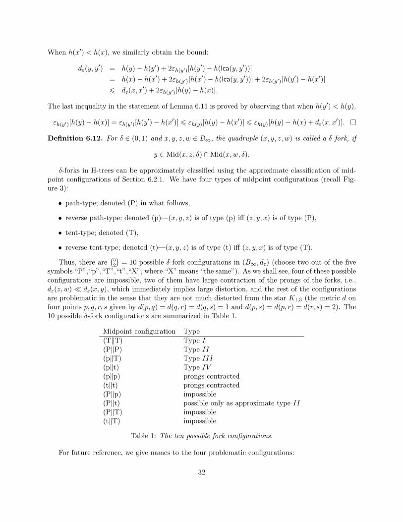
symbols “P”,“p”,“T”,“t”,“X”, where “X” means “the same”). As we shall see, four of these possibleconfigurations are impossible, two of them have large contraction of the prongs of the forks, i.e.,dε(z, w) dε(x, y), which immediately implies large distortion, and the rest of the configurationsare problematic in the sense that they are not much distorted from the star K1,3 (the metric d onfour points p, q, r, s given by d(p, q) = d(q, r) = d(q, s) = 1 and d(p, s) = d(p, r) = d(r, s) = 2). The10 possible δ-fork configurations are summarized in Table 1.

Midpoint configuration Type

(T‖T) Type I(P‖P) Type II(p‖T) Type III(p‖t) Type IV(p‖p) prongs contracted(t‖t) prongs contracted(P‖p) impossible(P‖t) possible only as approximate type II(P‖T) impossible(t‖T) impossible

Table 1: The ten possible fork configurations.

For future reference, we give names to the four problematic configurations:

32

Definition 6.13. For η, δ ∈ (0, 1), a δ-fork (x, y, z, w) of (B∞, dε) is called

• η-near Type I (configuration (T‖T)) in Table 1), if both (x, y, z) and (x, y, w) are η-neartent-type configurations;

• η-near Type II (configuration (P‖P) in Table 1), if both (x, y, z) and (x, y, w) are η-nearpath-type configurations;

• η-near Type III (configuration (p‖T) in Table 1), if (z, y, x) is η-near a path-type configura-tion and (x, y, w) is η-near a tent-type configuration, or vice versa;

• η-near Type IV (configuration (p‖t) in Table 1), if (z, y, x) is η-near a path-type configurationand (w, y, x) is η-near a tent-type configuration, or vice versa.

A schematic description of the four problematic configurations is contained in Figure 4.

x

y

z

wx

y

z

w

Type I Type II Type III Type IV

z

y

w

x

z

y

w

x

Figure 4: The four “problematic” types of δ-forks.

The following lemma is the main result of this section.

Lemma 6.14. Fix δ ∈(0, 1

70

)and assume that εn < 1

4 for all n ∈ N. If (x, y, z, w) is a δ-fork of (B∞, dε) then either it is 35δdε(x, y)-near one of the types I, II, III, IV , or we havedε(z, w) 6 2(35δ + εh0)dε(x, y), where h0 = minh(x), h(y), h(z), h(w).Remark 6.15. One can strengthen the statement of Lemma 6.14 so that in the first case the fork(x, y, z, w) is O(δdε(x, y)) near another fork (x′, y′, z′, w′) which is of (i.e. 0-near) one of the typesI, II, III, IV . This statement is more complicated to prove, and since we do not actually need itin what follows, we opted to use a weaker property which suffices for our purposes, yet simplifies(the already quite involved) proof.

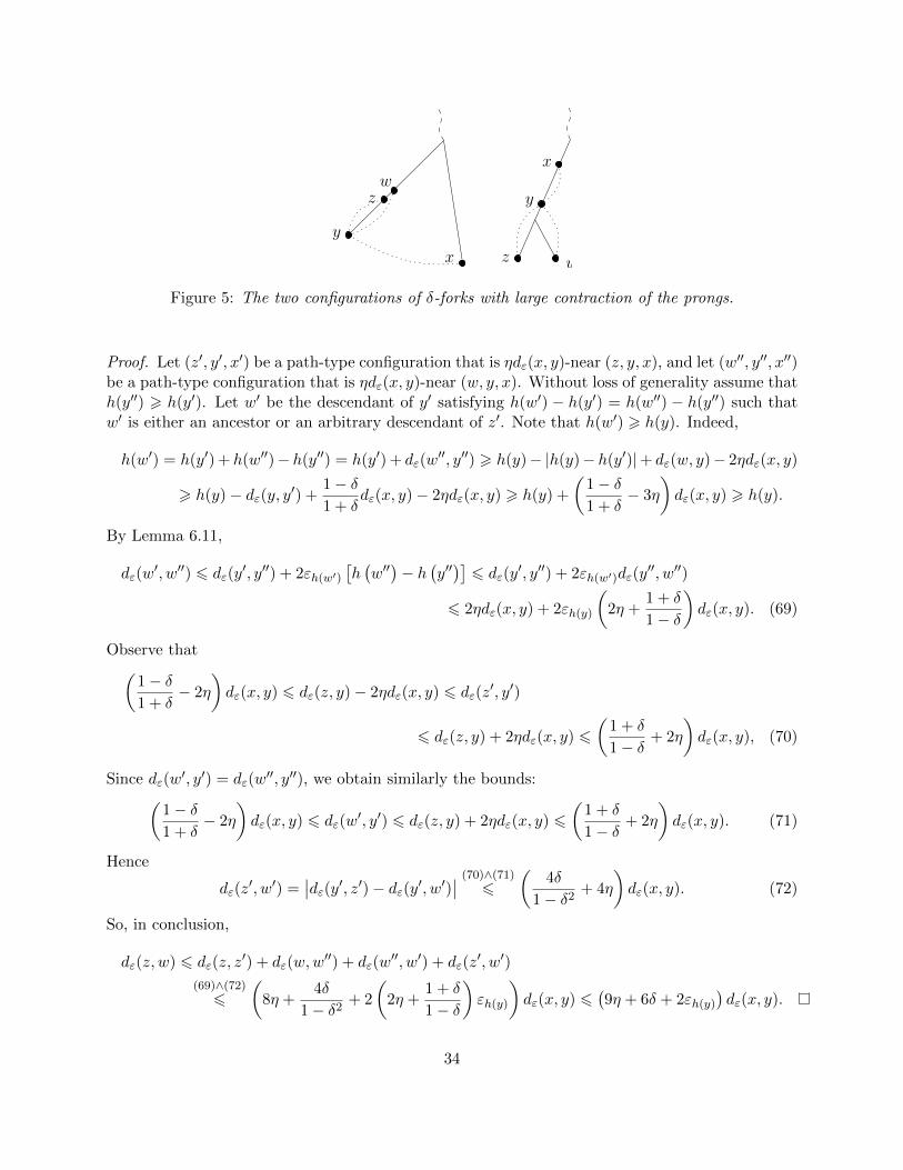
The proof of Lemma 6.14 proceeds by checking that the cases marked in Table 1 as “impossible”or “prongs contracted” are indeed so—see Figure 5 for a schematic description of the latter case.

We begin with the (p‖p) configuration.

Lemma 6.16. Let (x, y, z, w) be a δ-fork of (B∞, dε) and assume that both (z, y, x), and (w, y, x)are ηdε(x, y)-near path-type configurations. Then, assuming that maxδ, η < 1/8 and εn <

14 for

all n, we havedε(z, w) 6

(9η + 6δ + 2εh(y)

)dε(x, y).

33

x

y

zw

z

y

w

x

Figure 5: The two configurations of δ-forks with large contraction of the prongs.

Proof. Let (z′, y′, x′) be a path-type configuration that is ηdε(x, y)-near (z, y, x), and let (w′′, y′′, x′′)be a path-type configuration that is ηdε(x, y)-near (w, y, x). Without loss of generality assume thath(y′′) > h(y′). Let w′ be the descendant of y′ satisfying h(w′) − h(y′) = h(w′′) − h(y′′) such thatw′ is either an ancestor or an arbitrary descendant of z′. Note that h(w′) > h(y). Indeed,

h(w′) = h(y′) + h(w′′)− h(y′′) = h(y′) + dε(w′′, y′′) > h(y)− |h(y)− h(y′)|+ dε(w, y)− 2ηdε(x, y)

> h(y)− dε(y, y′) +1− δ1 + δ

dε(x, y)− 2ηdε(x, y) > h(y) +

(1− δ1 + δ

− 3η

)dε(x, y) > h(y).

By Lemma 6.11,

dε(w′, w′′) 6 dε(y

′, y′′) + 2εh(w′)

[h(w′′)− h

(y′′)]

6 dε(y′, y′′) + 2εh(w′)dε(y

′′, w′′)

6 2ηdε(x, y) + 2εh(y)

(2η +

1 + δ

1− δ

)dε(x, y). (69)

Observe that(1− δ1 + δ

− 2η

)dε(x, y) 6 dε(z, y)− 2ηdε(x, y) 6 dε(z

′, y′)

6 dε(z, y) + 2ηdε(x, y) 6

(1 + δ

1− δ + 2η

)dε(x, y), (70)

Since dε(w′, y′) = dε(w

′′, y′′), we obtain similarly the bounds:(1− δ1 + δ

− 2η

)dε(x, y) 6 dε(w

′, y′) 6 dε(z, y) + 2ηdε(x, y) 6

(1 + δ

1− δ + 2η

)dε(x, y). (71)

Hence

dε(z′, w′) =

∣∣dε(y′, z′)− dε(y′, w′)∣∣ (70)∧(71)

6

(4δ

1− δ2+ 4η

)dε(x, y). (72)

So, in conclusion,

dε(z, w) 6 dε(z, z′) + dε(w,w

′′) + dε(w′′, w′) + dε(z

′, w′)(69)∧(72)

6

(8η +

4δ

1− δ2+ 2

(2η +

1 + δ

1− δ

)εh(y)

)dε(x, y) 6

(9η + 6δ + 2εh(y)

)dε(x, y).

34

We next consider the (t‖t) configuration.

Lemma 6.17. Let (x, y, z, w) be a δ-fork of (B∞, dε). Assume that both (z, y, x) and (w, y, x) areηdε(x, y)-near tent-type configurations. Then, assuming that maxδ, η < 1/4, we have

dε(z, w) 6 (8η + 5δ)dε(x, y).

Proof. Let (z′, y′, x′) be a tent-type configuration that is ηdε(x, y)-near (z, y, x), and let (w′′, y′′, x′′)be a tent-type configuration that is ηdε(x, y)-near (w, y, x). Assume without loss of generality thath(y′′) − h(w′′) > h(y′) − h(z′). Let w be a point on the path between w′′ and y′′ such thath(y′′)− h(w) = h(y′)− h(z′). Then,

dε(w′′, w) = h(y′′)− h(w′′)− (h(y′)− h(z′)) = dε(y

′′, w′′)− dε(y′, z′)

6 dε(y, w)− dε(y, z) + 4ηdε(x, y) 6

(1 + δ

1− δ −1− δ1 + δ

+ 4η

)dε(x, y). (73)

By Lemma 6.9 we have dε(w, z′) 6 dε(y

′, y′′) 6 2ηdε(x, y). Hence we conclude that

dε(y, z) 6 dε(z, z′) + dε(w, z

′) + dε(w, w′′) + dε(w

′′, w)(73)

6

(4δ

1− δ2+ 8η

)dε(x, y).

Lemma 6.18. Let (x, y, z, w) be a δ-fork of B∞. Assume that (x, y, z) is ηdε(x, y)-near a path-typeconfiguration. Assume also that δ < 1/30, η < 1/10, and εn < 1/4 for all n. Then (x, y, w) is(2η + 21δ)dε(x, y)-near a path-type configuration, i.e., (x, y, z, w) is (2η + 21δ)dε(x, y)-near a typeII configuration.

Proof. Let (x′, y′, z′) be a path-type configuration which is ηdε(x, y)-near (x, y, z). By Theorem 6.4,either (x, y, w) or (w, y, x) must be 3δdε(x, z) 6 6

1−δdε(x, y) 6 7δdε(x, y)-near either a path-typeconfiguration or a tent-type configuration.

Suppose first that (x, y, w) is 7δdε(x, y)-near a tent-type configuration (x′′, y′′, w′′). In this case,x′′ is an ancestor of y′′ and h(y′′)− h(x′′) = dε(x

′′, y′′) > (1− 14δ)dε(x, y). At the same time, y′ isan ancestor of x′ and h(x′)− h(y′) = dε(x

′, y′) > (1− 2η)dε(x, y). So,

2(η + 7δ)dε(x, y) > dε(y′′, y′) + dε(x

′, x′′) > h(y′′)− h(x′′) + h(x′)− h(y′) > 2(1− η − 7δ)dε(x, y),

which is a contradiction since η + 7δ < 1/2.Next suppose that (w, y, x) is 7δdε(x, y)-near a path-type configuration (w′′, y′′, x′′). Then

|h(x′)− h(x′′)| 6 dε(x′, x′′) 6 (η + 7δ)dε(x, y). So,

(η + 7δ)dε(x, y) > dε(y′, y′′) > h(y′′)− h(y′)

= (h(y′′)− h(x′′)) + (h(x′′)− h(x′)) + h(x′)− h(y′) > 0− (η + 7δ)dε(x, y) + (1− 2η)dε(x, y),

which is a contradictionLastly, suppose that (w, y, x) is 7δdε(x, y)-near a tent-type configuration (w′′, y′′, x′′). Note that

|h(y′)− h(y′′)| 6 dε(y′, y′′) 6 (η + 7δ)dε(x, y). So, h(y′) > h(y′′)− (η + 7δ)dε(x, y). Also,

h(y′′)− h(w′′) = dε(y′′, w′′) > dε(y, w)− 14δdε(x, y) >

(1− δ1 + δ

− 14δ

)dε(x, y) > (η + 7δ)dε(x, y).

35

Consider the point w defined as the ancestor of y′ at distance h(y′′)−h(w′′)− (η+ 7δ)dε(x, y) fromy′. Let also w′′′ be the ancestor of y′′ at distance h(y′′) − h(w′′) − (η + 7δ)dε(x, y) from y′′. ByLemma 6.9, we have dε(w, w

′′′) 6 dε(y′, y′′) 6 (η + 7δ)dε(x, y). Therefore,

dε(w, w) 6 dε(w, w′′′) + dε(w

′′′, w′′) + dε(w′′, w) 6 (2η + 21δ)dε(x, y).

Hence (x, y, w) is (2η + 21δ)dε(x, y)-near the path-type configuration (x′, y′, w).

Lemma 6.19. Let (x, y, z, w) be a δ-fork of B∞. Assume that (x, y, z) is ηdε(x, y)-near a tent-type configuration. Assume also that η < 1/10 and εn < 1/4 for all n. Then (w, y, x) cannot beηdε(x, y)-near a tent-type configuration.

Proof. Let (x′, y′, z′) be a tent type configuration that is ηdε(x, y)-near (x, y, z). Suppose for contra-diction that there exists a tent type configuration (w′′, y′′, x′′) that is ηdε(x, y)-near (w, y, x). Notethat h(y′′) > h(y′)−dε(y′, y′′) > h(y′)−2ηdε(x, y) and h(y′)−h(x′) > (1−2η)dε(x, y) > 2ηdε(x, y).Let x∗ be the ancestor of y′ at distance h(y′) − h(x′) − 2ηdε(x, y) from y′, and let x be the an-cestor of y′′ at distance h(y′) − h(x′) − 2ηdε(x, y) from y′′. An application of Lemma 6.9 yieldsthe estimate dε(x, x

∗) 6 dε(y′, y′′) 6 2ηdε(x, y). But, since h(x′′) > h(y′′), we also know that

dε(x, x′′) > h(y′′)− h(x) = dε(y

′, x′)− 2ηdε(x, y). Hence,

2ηdε(x, y) > dε(x, x∗) > dε(x, x

′′)−dε(x∗, x′)−dε(x′, x′′) > dε(x′, y′)−6ηdε(x, y) > (1−8η)dε(x, y),

which is a contradiction, since η < 1/10.

Proof of Lemma 6.14. Since (x, y, z, w) is a δ-fork, by Theorem 6.4, both (x, y, z) and (x, y, w) are7δdε(x, y)-near a tent-type configuration, a path-type configuration, or the corresponding reverseconfigurations. We have 10 possible combinations of these pairs, as appearing in Table 1. Byapplying Lemmas 6.18 and 6.19 with η = 7δ, we rule out three of these configurations, and a fourthconfiguration is possible but only as 35δdε(x, y)-near a type II configuration.

We are left with six possible configurations. By applying Lemmas 6.16 and 6.17 with η = 7δwe conclude that in two of those configurations we have dε(w, z) 6 (69δ + 2εh0)dε(x, y), and therest are configurations that are 7δdε(x, y)-near one of the types I–IV .

6.2.3 Classification of approximate 3-paths

We start with the following natural notion:

Definition 6.20. For x0, x1, x2, x3 ∈ B∞ the quadruple (x0, x1, x2, x3) is called a (1+δ)-approximateP3 if there exists L > 0 such that for every 0 6 i 6 j 6 3 we have

(j − i)L 6 dε(xi, xj) 6 (1 + δ)(j − i)L.

Note that in this case x1 ∈ Mid(x0, x2, δ) and x2 ∈ Mid(x1, x3, δ).

As in the case of δ-forks, there are 10 possible concatenations of two midpoints configurations(path-type or tent-type): P-P, P-p, P-T, P-t, p-P, p-T, p-t, T-T, T-t, t-T (the midpoint config-urations p-p, P-p, t-p, T-p, p-P, t-P, T-P, t-t, T-t, t-T are respectively such concatenations withthe order of x0, x1, x2, x3 reversed). We will rule out some of these possibilities, and obtain somestronger properties for the rest. See Table 2.

As in the case of δ-forks, it will be beneficial to give names to three special types approximate3-paths:

36

Midpoint configuration Reverse configuration Type

(P-P) (p-p) type A(P-p) (P-p) impossible(P-T) (t-p) impossible(P-t) (T-p) type B(p-P) (p-P) impossible(p-T) (t-P) type C(p-t) (T-P) impossible(T-T) (t-t) possible only as type C(T-t) (T-t) impossible(t-T) (t-T) impossible

Table 2: The possible configurations of 3 paths.

Definition 6.21. For x0, x1, x2, x3 ∈ B∞ and η > 0, a quadruple (x0, x1, x2, x3) is called:

• η-near a type A configuration if both (x0, x1, x2) and (x1, x2, x3) are η-near path-type config-urations,

• η-near a type B configuration if (x0, x1, x2) is η-near a path-type configuration, and (x3, x2, x1)is η-near tent-type configuration,

• η near type C configuration if (x2, x1, x0) is η-near a path-type configuration, and (x1, x2, x3)is η-near a tent-type configuration.

See also Figure 6.

Type CType Bx0

x1 x2

x3

x0

x1

x2

x3

Type A

x1

x2x3

x0

Figure 6: The three possible types of approximate 3-paths.

The following lemma is the main result of this subsection.

Lemma 6.22. Assume that εn < 14 for all n and fix δ < 1/200. Assume that (x0, x1, x2, x3)

is a (1 + δ)-approximate P3. Then either (x0, x1, x2, x3) or (x3, x2, x1, x0) is 35δdε(x0, x1)-near aconfiguration of type A, B or C.

37

The proof of Lemma 6.22 is again a case analysis that examines all 10 possible ways (up tosymmetry) to concatenate two midpoint configurations. The proof is divided into a few lemmasaccording to the cases, and is completed at the end of this subsection.

Lemma 6.23. Assume that εn <14 for all n and that (x0, x1, x2, x3) is a (1 + δ)-approximate P3

such that (x0, x1, x2) is ηdε(x0, x1)-near a path-type configuration. If maxδ, η < 1/200 then either(x1, x2, x3) is 7δdε(x0, x1)-near a path-type configuration (type A), or (x3, x2, x1) is 7δdε(x0, x1)-near a tent-type configuration (type B).

Proof. Due to Theorem 6.4 we only need to rule out the possibility that (x3, x2, x1) is 7δdε(x1, x2)-near a path-type configuration, or that (x1, x2, x3) is 7δdε(x1, x2)-near a tent-type configuration.Let (x′0, x

′1, x′2) be a path-type configuration that is ηdε(x0, x1)-near (x0, x1, x2).

Suppose first that (x3, x2, x1) is 7δdε(x1, x2)-near the path-type configuration (x′′3, x′′2, x′′1). Since

h(x′1) > h(x′2) and h(x′′2) > h(x′′1) we have,

|h(x1)− h(x2)| 6 |h(x1)− h(x′1)|+(h(x′1)− h(x′2)

)+ |h(x′2)− h(x2)|

6 dε(x1, x′1) +

(h(x′1)− h(x′2)

)+ dε(x

′2, x2) 6 2ηdε(x0, x1) +

(h(x′1)− h(x′2)

), (74)

and similarly,

|h(x1)− h(x2)| 6 |h(x1)− h(x′′1)|+(h(x′′2)− h(x′′1)

)+ |h(x′′2)− h(x2)|

6 dε(x1, x′′1) +

(h(x′′2)− h(x′′1)

)+ dε(x

′2, x2) 6 14δdε(x0, x1) +

(h(x′′2)− h(x′′1)

). (75)

By summing (74) and (75) we obtain the bound

2|h(x1)− h(x2)| 6 (2η + 14δ) dε(x0, x1) + dε(x′1, x′′1) + dε(x

′2, x′′2) 6 (4η + 28δ) dε(x0, x1).

Thus|h(x1)− h(x2)| 6 (2η + 14δ)dε(x0, x1). (76)

Since x′0 is a descendant of x′1,

|h(x0)− h(x1)− dε(x0, x1)| 6 |h(x′0)− h(x′1)− dε(x0, x1)|+ 2ηdε(x0, x1)

= |dε(x′0, x′1)− dε(x0, x1)|+ 2δdε(x0, x1) 6 4ηdε(x0, x1). (77)

Similarly, since x′′3 is a descendant of x′′2,

|h(x3)− h(x2)− dε(x0, x1)| 6 |h(x′′3)− h(x′′2)− dε(x0, x1)|+ 14δdε(x1, x2)

= |dε(x′′3, x′′2)− dε(x0, x1)|+ 14δdε(x0, x1) 6 28δdε(x0, x1). (78)

Hence,

|h(x′′3)− h(x′0)| 6 |h(x′′3)− h(x3)|+ |h(x3)− h(x2)− dε(x0, x1)|+ |h(x2)− h(x1)|+|h(x0)− h(x1)− dε(x0, x1)|+ |h(x0)− h(x′0)|

(76)∧(77)∧(78)

6 dε(x′′3, x3) + 28δdε(x0, x1) + (2η + 14δ)dε(x0, x1) + 4ηdε(x0, x1) + dε(x0, x

′0)

6 (49δ + 7η)dε(x0, x1). (79)

38

We record for future reference the following consequence of (76) and (79):

minh(x′0), h(x′′3) −minh(x′1), h(x′′2) 6 maxh(x′0)− h(x′1), h(x′0)− h(x′′2)

(79)

6 maxdε(x

′0, x′1), h(x′′3)− h(x′′2) + (49δ + 7η)dε(x0, x1)

6 max

(1 + 2η)dε(x0, x1), dε(x

′′3, x′′2) + (49δ + 7η)dε(x0, x1)

6 (1 + 64δ + 7η)dε(x0, x1). (80)

We next claim thatlca(x′0, x

′′3) = lca(x′1, x

′′2). (81)

Indeed, since x′1 is an ancestor of x′0 and x′′2 is an ancestor of x′′3, if lca(x′0, x′′3) 6= lca(x′1, x

′′2) then

either x′1 is a descendant of x′′2, or x′′2 is a descendant of x′1. If x′1 is a descendant of x′′2 then

(η + 7δ)dε(x0, x1) > dε(x′1, x′′1) > dε(x

′′2, x′1) > dε(x2, x1)− (η + 7δ)dε(x0, x1)

>1

1 + δdε(x0, x1)− (η + 7δ)dε(x0, x1),

which is a contradiction since δ, η < 1/200. Similarly, if x′′2 is a descendant of x′1 then

(η + 7δ)dε(x0, x1) > dε(x′2, x′′2) > dε(x

′′2, x′1) >

1

1 + δdε(x0, x1)− (η + 7δ)dε(x0, x1),

arriving once more at a contradiction. This proves (81).Now,

3

1 + δdε(x0, x1) 6 dε(x0, x3)

6 dε(x′′3, x′0) + (η + 7δ)dε(x0, x1)

(79)

6 2εminh(x′0),h(x′′3 )[minh(x′0), h(x′′3) − h(lca(x′0, x

′′3))]

+ (8η + 56δ)dε(x0, x1)

(81)= 2εminh(x′0),h(x′′3 )

[minh(x′1), h(x′′2) − h(lca(x′1, x

′′2))]

+ (8η + 56δ)dε(x0, x1)

+ 2εminh(x′0),h(x′′3 )[minh(x′0), h(x′′3) −minh(x′1), h(x′′2)

](80)

6 2εminh(x′1),h(x′′2 )[minh(x′1), h(x′′2) − h(lca(x′1, x

′′2))]

+

(8η + 56δ +

1 + 64δ + 7η

2

)dε(x0, x1) (82)

6 dε(x′1, x′′2) +

(1

2+ 88δ + 12η

)dε(x0, x1)

6

(3

2+ 96δ + 13η

)dε(x0, x1), (83)

where in (82) we used minh(x′0), h(x′′3) > minh(x′1), h(x′′2) and εminh(x′0),h(x′′3 ) < 1/4. Sincemaxη, δ < 1/200, the bound (83) is a contradiction.

39

Next suppose that (x1, x2, x3) is 7δdε(x0, x1)-near a tent-type configuration (x′′1, x′′2, x′′3). Since

h(x′2) 6 h(x′1) and h(x′′2) > h(x′′1), we have

|h(x1)− h(x2)| 6 |h(x1)− h(x′1)|+(h(x′1)− h(x′2)

)+ |h(x′2)− h(x2)|

6 dε(x1, x′1) +

(h(x′1)− h(x′2)

)+(h(x′′2)− h(x′′1)

)+ dε(x

′2, x2)

6 dε(x1, x′1) + dε(x

′1, x′′1) + dε(x

′2, x′′2) + dε(x

′2, x2)

6 (4η + 14δ)dε(x0, x1). (84)

On the other hand, x′′1 is an ancestor of x′′2, and therefore we have(1

1 + δ− 14δ

)dε(x0, x1) 6 dε(x

′′1, x′′2) = h(x′′2)− h(x′′1)

6 |h(x1)− h(x2)|+ 14δdε(x0, x1)(84)

6 (4η + 28δ)dε(x0, x1), (85)

which is a contradiction since maxη, δ < 1/200.

Lemma 6.24. Assume that εn < 14 for all n and that (x0, x1, x2, x3) is a (1 + δ)-approximate

P3 such that (x2, x1, x0) is ηdε(x0, x1)-near a path-type configuration. If maxδ, η < 1/200 theneither (x3, x2, x1) is 7δdε(x0, x1)-near a path-type configuration (reverse type A), or (x1, x2, x3) is7δdε(x0, x1)-near a tent-type configuration (type C).

Proof. Let (x′2, x′1, x′0) be in path-type configuration that is ηdε(x0, x1)-near (x2, x1, x0). First,

assume for contradiction that (x3, x2, x1) is 7δdε(x1, x2)-near a tent-type configuration (x′′3, x′′2, x′′1).

Then h(x′′1) > h(x′′2), where as h(x′2) − h(x′1) = dε(x′2, x′1). Arguing as in (84), it follows that

|h(x1)−h(x2)| 6 (2η+28δ)dε(x0, x1), and we arrive at a contradiction by arguing similarly to (85).Next, assume for contradiction that (x1, x2, x3) is 7δdε(x1, x2)-near a path-type configuration

(x′′1, x′′2, x′′3). Then h(x′′1) − h(x′′2) = dε(x

′′1, x′′2), whereas h(x′2) − h(x′1) = dε(x

′1, x′2). By summing

these two identities, we arrive at a contradiction as follows:(2

1 + δ− 2η − 14δ

)dε(x0, x1) 6 dε(x

′1, x′2) + dε(x

′′1, x′′2) =

(h(x′2)− h(x′′2)

)+(h(x′′1)− h(x′1)

)6 dε(x

′2, x′′2) + dε(x

′1, x′′1) 6 (2η + 14δ)dε(x0, x1).

Lemma 6.25. Assume that εn <14 for all n and that (x0, x1, x2, x3) is a (1 + δ)-approximate P3

such that (x0, x1, x2) is ηdε(x0, x1)-near a tent-type configuration. If maxδ, η < 1/200 then either(x2, x1, x0) is (14δ + 3η)dε(x0, x1)-near a path-type configuration and (x1, x2, x3) is 7δdε(x1, x2)-near a tent-type configuration (type C), or (x3, x2, x1) is 7δdε(x0, x1)-near a path-type configuration(reverse type B).

Proof. Let (x′0, x′1, x′2) be a tent-type configuration that is ηdε(x0, x1)-near (x0, x1, x2). First,

suppose that (x1, x2, x3) is 7δdε(x1, x2)-near a tent-type configuration (x′′1, x′′2, x′′3). Note that

|h(x′1) − h(x′′1)| 6 dε(x′1, x′′1) 6 (η + 7δ)dε(x0, x1). So, let x′′0 be an ancestor of x′′1 at distance

h(x′1) − h(x′0) − (η + 7δ)dε(x0, x1) ∈ [0, h(x′′1)] from x′′1, and let x∗0 be an ancestor of x′1 at dis-tance h(x′1) − h(x′0) − (η + 7δ)dε(x0, x1) from x′1. Then h(x′1) − h(x∗0) = h(x′′1) − h(x′′0) anddε(x

∗0, x′0) 6 (η + 7δ)dε(x0, x1). By Lemma 6.9,

dε(x0, x′′0)− (2η + 7δ)dε(x0, x1 6 dε(x0, x

′′0)− dε(x∗0, x′0)− dε(x′0, x0) 6 dε(x

∗0, x′′0)

6 dε(x′1, x′′1) 6 (η + 7δ)dε(x0, x1).

40

Hence (x′′2, x′′1, x′′0) is a path-type configuration that is (14δ + 3η)dε(x0, x1)-near (x2, x1, x0).

Next assume for contradiction that (x3, x2, x1) is 7δdε(x1, x2) near a tent-type configuration(x′′3, x

′′2, x′′1). Then

(1− 15δ) dε(x0, x1) 6

(1

1 + δ− 14δ

)dε(x0, x1) 6 h(x′′2)− h(x′′3) 6 (1 + 15δ)dε(x0, x1), (86)

and

(1− δ − 2η) dε(x0, x1) 6

(1

1 + δ− 2η

)dε(x0, x1) 6 h(x′1)− h(x′0) 6 (1 + δ + 2η)dε(x0, x1). (87)

So, let x##3 be an ancestor of x′′2 at distance h(x′′2)− h(x′′3)− (16δ + 2η) dε(x0, x1) ∈ [0, h(x′′2)] from

x′′2, and let x#0 be an ancestor of x′1 at distance h(x′′2) − h(x′′3) − (16δ + 2η) dε(x0, x1) ∈ [0, h(x′1)]

from x′1. Then

dε(x′′3, x

##3 ) 6 (16δ + 2η) dε(x0, x1), (88)

and

dε(x′0, x

#0 ) =

∣∣∣h(x′0)− h(x#0 )∣∣∣ =

∣∣h(x′0)−(h(x′1)− h(x′′2) + h(x′′3) + (16δ + 2η) dε(x0, x1)

)∣∣(86)∧(87)

6 2(16δ + 2η)dε(x0, x1). (89)

Moreover, h(x1)− h(x#0 ) = h(x′′2)− h(x##

3 ), so by Lemma 6.9 we have(3

1 + δ− 55δ − 7η

)dε(x0, x1) 6 dε(x0, x3)− (55δ + 7η)dε(x0, x1)

(88)∧(89)

6 dε(x#0 , x

##3 )

6 dε(x′1, x′′2) 6 (1 + 8δ + η)dε(x0, x1),

which is a contradiction since maxδ, η < 1/200.Lastly, assume for contradiction that (x1, x2, x3) is 7δdε(x1, x2)-near a path-type configuration

(x′′1, x′′2, x′′3). Then since h(x′1) 6 h(x′2) we have(

1

1 + δ− 14δ

)dε(x0, x1) 6 dε(x

′′1, x′′2) = h(x′′1)− h(x′′2) 6

(h(x′′1)− h(x′′2)

)+(h(x′2)− h(x′1)

)6 dε(x

′′1, x′1) + dε(x

′′2, x′2) 6 (14δ + 2η)dε(x0, x1),

a contradiction.

Lemma 6.26. Assume that εn < 14 for all n and that (x0, x1, x2, x3) is a (1 + δ)-approximate

P3 such that (x2, x1, x0) is ηdε(x0, x1)-near a tent-type configuration. If maxδ, η < 1/200 then(x1, x2, x3) cannot be 7δdε(x0, x1) near a tent-type configuration.

Proof. Let (x′2, x′1, x′0) be a tent-type configuration that is ηdε(x0, x1)-near (x2, x1, x0). Suppose

for contradiction that (x1, x2, x3) is 7δdε(x0, x1)-near a tent-type configuration (x′′1, x′′2, x′′3). Then

h(x′1) − h(x′2) = dε(x′1, x′2), whereas h(x′′2) − h(x′′1) = dε(x

′′1, x′′2). Taking the sum of these two

inequalities we conclude that

dε(x′′1, x′′2) + dε(x

′1, x′2) 6 dε(x

′1, x′′1) + dε(x

′2, x′′2) 6 (2η + 14δ)dε(x0, x1).

At the same time,(

21+δ − 2η − 14δ

)dε(x0, x1) 6 dε(x

′′1, x′′2) + dε(x

′1, x′2), which leads to the desired

contradiction.

41

Proof of Lemma 6.22. Since (x0, x1, x2, x3) is a (1+δ)-approximate P3, we have x1 ∈ Mid(x0, x2, δ),and x2 ∈ Mid(x1, x3, δ). Since the assumptions of Theorem 6.4 hold, we can apply with η = 7δLemmas 6.23, 6.24, 6.25, 6.26, and conclude that either (x0, x1, x2, x3) or (x3, x2, x1, x0) must be35δdε(x0, x1)-near a configuration of type A, B or C.

6.3 Nonembeddability of vertically faithful B4

In what follows we need some standard notation on trees. As before, Bn is the complete binarytree of height n; the root of Bn is denoted by r. Denote by I(Bn) the set of internal vertices of Bn,i.e., vertices of Bn which are not the root or a leaf. For a vertex v in r ∪ I(Bn) we denote byv0 and v1 its children. For α ∈ 0, 1∗ (the set of finite sequences of ’0’ and ’1’) and a ∈ 0, 1 wedenote by vαa = (vα)a.

The aim of the current section is to prove the following lemma.

Lemma 6.27. Fix 0 < δ < 1/400 and let f : B4 → (B∞, dε) be a (1 + δ)-vertically faithfulembedding. Then the distortion of f satisfies

dist(f) >1

500δ + εh0,

where h0 = minx∈B4 h(f(x)).

The proof of Lemma 6.27 is by a contradiction. By Lemma 6.14, assuming the distortion off is small, all the δ-forks in the (1 + δ)-vertically faithful embedding must be of types I–IV . Byexploring the constrains implied by Lemma 6.22 on how those δ-forks can be “stitched” together,we reach the conclusion that they are sufficiently severe to force any vertically faithful embeddingof B4 to have a large contraction, and therefore high distortion.

Fix f : B4 → (B∞, dε). For u ∈ I(B4) we denote by F(u) the fork in which u is the centerpoint, i.e., if v be the parent of u in B4, then

F(u)def= (f(v), f(u), f(u0), f(u1)).

We shall assume from now on that f satisfies the assumptions of Lemma 6.27, i.e., that it satisfies (8)with D = 1 + δ for some δ < 1/400 and λ > 0.

Lemma 6.28. Fix u ∈ B4 with h(u) ∈ 1, 2. If the fork F(u) is 37δλ-near a type I or type IIIconfiguration, then there exists w ∈ I(B4) satisfying

dε(f(w0), f(w1)) 6 (170δ + εh0) · 2λ. (90)

Proof. Let v be the parent of u. Hence, (f(v), f(u), f(u0), f(u1)) is 35δ(1 + δ)λ-near a type I or atype III configuration. Assume first that (f(v), f(u), f(u0), f(u1)) is 37δλ-near a type I configu-ration. If both (f(u0), f(u), f(v)) and (f(u1), f(u), f(v)) were 37δλ-near a path type configurationthen by Lemma 6.16 (with η = 37δ) we would have

dε(f(u0), f(u1)) 6 (339δ + 2εh0)(1 + δ)λ 6 (170δ + εh0) · 2λ, (91)

proving (90) with w = u. The same conclusion holds when (f(v), f(u), f(u0), f(u1)) is 37δλ-neara type III configuration: in this case without loss of generality (f(v), f(u), f(u0)) is 37δλ-near

42

a tent-type configuration and (f(u1), f(u), f(v)) is 37δλ-near a path-type configuration. UsingLemma 6.16 as above we would arrive at the conclusion (91) if (f(u0), f(u), f(v)) were 37δλ-near apath-type type configuration. Thus, in both the type I and type III cases of Lemma 6.28 we mayassume that (f(v), f(u), f(u0)) is 37δλ-near a tent-type configuration, and that, by Lemma 6.8,(f(v), f(u), f(u0)) is not 37δλ-near a path-type configuration, and (f(u0), f(u), f(v)) is not 37δλ-near a path-type configuration or a tent-type configuration.

By Lemma 6.22 (and Table 2) (f(u0c), f(u0), f(u), f(v)) must be 35δ(1 + δ)λ-near a type Bconfiguration for both c ∈ 0, 1. This means that (f(u0c), f(u0), f(u)) are both 35δ(1 + δ)λ-near a path-type configuration, and so by Lemma 6.16 (with η = 35δ(1 + δ)) we deduce thatdε(f(u00), f(u01)) 6 (170δ + εh0) · 2λ.

Lemma 6.29. Fix u ∈ B4 with h(u) ∈ 1, 2. If F(u) is 37δλ-near a type II configuration thenfor both b ∈ 0, 1 either F(ub) is 99δλ-near a type II configuration, or dε(f(ub0), f(ub1)) 6 400δλ.

Proof. Let v be the parent of u. For both c ∈ 0, 1 we know that (f(v), f(u), f(u0), f(u0c))is a (1 + δ)-approximate P3, and therefore by Lemma 6.22 either (f(v), f(u), f(u0), f(u0c)) or(f(u0c), f(u0), f(u), f(v)) is 35δ(1 + δ)λ-near a configuration of type A, B or C. Note that since(f(v), f(u), f(u0)) is assumed to be 37δλ-near a path-type configuration, we rule out the possibilitythat (f(v), f(u), f(u0), f(u0c)) is 35δ(1 + δ)λ-near a configuration of type C, since otherwise both(f(v), f(u), f(u0)) and (f(u0), f(u), f(v)) would be 37δλ-near path-type configurations, contra-dicting Lemma 6.8. For the same reason we rule out the possibility that (f(u0c), f(u0), f(u), f(v))is 35δ(1 + δ)λ-near a configuration of type A or type B. An inspection of the three remain-ing possibilities shows that either (f(u), f(u0), f(u0c)) is 37δλ-near a path-type configuration, or(f(u0c), f(u0), f(u)) is 37δλ-near a tent-type configuration.

Now,

• If for both c ∈ 0, 1 we have that (f(u), f(u0), f(u0c)) is 37δλ-near a path-type configuration,then F(u0) is 37δλ-near a type II configuration.

• If for both c ∈ 0, 1 we have that (f(u0c), f(u0), f(u)) are 37δλ-near a tent-type configura-tion, then by Lemma 6.17 we have dε(f(u01), f(u00)) 6 400δ.

• By Lemma 6.18, the only way that (f(u), f(u0), f(u00)) could be 37δλ-near a path type con-figuration while at the same time (f(u01), f(u0), f(u)) is 37δλ-near a tent-type configuration(or vice versa), is that F(u0) is 99δλ-near a type II configuration.

Lemma 6.30. Fix u ∈ B4 with h(u) ∈ 1, 2. If F(u) is 35δ(1 + δ)λ-near a type IV configuration,then there exists b ∈ 0, 1 such that F(ub) is 37δλ-near a type II configuration.

Proof. Let v be the parent of u. Without loss of generality (f(u0), f(u), f(v)) is 35δ(1 + δ)λ-near atent-type configuration. By Lemma 6.22 (using Lemma 6.8 to rule out the remaining possibilities),this means that for both c ∈ 0, 1 the quadruple (f(u0c), f(u0), f(u), f(v)) is 35δ(1 + δ)2λ-near atype C configuration, and therefore F(u0) is 35δ(1 + δ)2λ near a type II configuration.

Lemma 6.31. Fix u ∈ B4 with h(u) ∈ 0, 1, 2. If F(u0) and F(u1) are both 99δλ-near type a IIconfiguration then dε(f(u0), f(u1)) 6 1000δλ.

43

Proof. By our assumptions, (f(u), f(u0), f(u00)) is 99δλ-near a path type configuration (u′, u′0, u′00)

and (f(u), f(u1), f(u10)) is 99δλ-near a path-type configuration (u′′, u′′1, u′′10). We may assume

without loss of generality that h(u′′) − h(u′1) 6 h(u′) − h(u′0). We may therefore consider theancestor u∗1 of u′ such that h(u′)−h(u∗1) = h(u′′)−h(u′′1), implying in particular that h(u∗1) > h(u′0)(recall that u′0 is an ancestor of u′, and u′′1 is ancestor of u′′). By Lemma 6.9 we have

dε(u∗1, u′′1) 6 dε(u

′, u′′) 6 198δλ. (92)

Hence,

h(u′)− h(u∗1) = dε(u′, u∗1)

(92)

> dε(u′, u′′1)− 198δλ > dε(f(u), f(u1))− 394δλ > (1− 394δ)λ. (93)

But, we also know that

h(u′)− h(u′0) = dε(u′, u′0) 6 dε(f(u), f(u0)) + 198δλ 6 (1 + 200δ)λ. (94)

It follows from (93) and (94) that dε(u′0, u∗1) = h(u∗1)− h(u′0) 6 601δλ. Therefore,

dε(f(u1), f(u0)) 6 dε(f(u0), u′0) + dε(u′0, u∗1) + dε(u

∗1, u′′1) + dε(u

′′1, f(u1)) = 1000δλ.

Proof of Lemma 6.27. We may assume that for all u ∈ I(B4) the fork F(u) is 35δ(1 + δ)λ-near aconfiguration of type I, II, III, or IV . Indeed, otherwise the proof is complete by Lemma 6.14.If F(r0) is 35δ(1 + δ)λ-near a type I or type III configuration, then by Lemma 6.28 the proof iscomplete. If F (r0) is 35δ(1 + δ)λ-near a type IV configuration then by Lemma 6.30 there existsb ∈ 0, 1 such that F (r0b) is 37δλ-near a type II configuration. It therefore remains to deal withthe case in which for some u ∈ r0, r0b the fork F(u) is 37δλ-near a type II configuration. ApplyingLemma 6.29, either we are done, or both F(u0) and F(u1) are 99δλ-near a type II configuration,but then by Lemma 6.31 the proof of Lemma 6.27 is complete.

6.4 Nonembeddability of binary trees

We are now in position to complete the proof of Theorem 1.10.

Proof of Theorem 1.10. Write εn = 1/s(n), and ε = εn∞n=0. Thus εn∞n=0 is non-increasing,nεn∞n=0 is non-decreasing, and εn 6 1/4. We can therefore choose the metric space (X, dX) =(B∞, dε). The identity embedding of Bn into the top n-levels of B∞ shows that cX(Bn) 6 s(n). Itremains to prove the lower bound on cX(Bn). To this end take an arbitrary injection f : Bn → Xsatisfying dist(f) 6 s(n), and we will now prove that

dist(f) > s

(⌊n

40s(n)

⌋)(1− Cs(n) log s(n)

log n

). (95)

By adjusting the constant C in (95), we may assume below that n is large enough, say, n > 100.Write h0 = bn/(40s(n))c and define X>h0 = x ∈ B∞ : h(x) > h0. We claim that there existsa complete binary subtree T ⊆ Bn of height at least dn/3e, such that we have f(T ) ⊆ X>h0 .Indeed, let hmin = minh(x) : x ∈ f(Bn) and hmax = maxh(x) : x ∈ f(Bn). If hmin > h0

then f(Bn) ⊆ X>h0 , and we can take T = Bn. So assume that hmin < h0. Since f is aninjection it must satisfy hmax > n. Hence ‖f‖Lip > hmax−hmin

2n > n−h02n > 1

4 . Since dist(f) 6 s(n)

44

we conclude that ‖f−1‖Lip 6 4s(n). It follows that, since diam(X r X>h0) 6 2h0, we havediam

(f−1(X rX>h0)

)6 8h0s(n) 6 n/5. If the top dn/3e levels of Bn are mapped into X>h0 then

we are done, so assume that there exists u ∈ f−1(X r X>h0) of depth at most 6 dn/3e. In thiscase f−1(X rX>h0) must be contained in the first dn/3e+ n/5 < 2n/3− 1 levels of Bn, so we cantake T to be any subtree of Bn contained in the last dn/3e levels of Bn.

Fix δ ∈ (0, 1). By Theorem 1.14 (with t = 4, D = s(n) and ξ = δ), there exists a universalconstant κ > 0 such that if n > s(n)κ/δ then there exists a mapping φ : B4 → Bn with dist(φ) 6 1+δ

such that f φ is a (1 + δ)-vertically faithful embedding of B4 into X>h0 . Choosing δ = κ log s(n)logn ,

by increasing C in (95) if necessary, we may assume that δ < 1/400. Lemma 6.27 then implies

(1 + δ) dist(f) > dist(f φ) >1

500δ + εh0=

1

500κ log s(n)logn + 1

s(bn/(40s(n))c).

The deduction of (7) from (6) is a simple exercise: if s(n) = o(log n/ log logn) then we have(s(n) log s(n))/ log n = o(1). The desired claim will then follow once we check that

lim supn→∞

s (bn/(40s(n))c)s(n)

= 1. (96)

Indeed, if (96) failed then there would exist ε0 ∈ (0, 1) and n0 ∈ N such that for all n > n0,

s (bn/ log nc) 6 s (bn/(40s(n))c) 6 (1− ε0)s(n). (97)

Iterating (97), it would follow that s(nj) > nΩ(1)j for some subsequence nj∞j=1, a contradiction.

Proof of Theorem 1.12. The proof is identical to the above argument: all one has to notice isthat when s(n) = D for all n ∈ N the resulting metric dε on B∞ is D-equivalent to the originalshortest path metric on B∞. In this case, if cX(Bn) 6 D − ε then the bound (95) implies thatn 6 DCD2/ε.

7 Discussion and open problems

A very interesting question that arises naturally from Theorem 1.3 and is also a part of the Ribeprogram, is finding a metric characterization of q-smoothness. A Banach space (X, ‖ · ‖X) is calledq-smooth if it admits an equivalent norm ||| · ||| such that there is a constant S > 0 satisfying:

|||x||| = 1 ∧ y ∈ X =⇒ |||x+ y|||+ |||x− y|||2

6 1 + S|||y|||q.

A Banach space X is p-convex if and only if its dual space X∗ is q-smooth, where 1p + 1

q = 1 [17].It is known that a Banach space X is p-convex for some p <∞ (i.e., superreflexive) if and only ifit is q-smooth for some q > 1 (this follows from [10, 29]). Hence Bourgain’s metric characterizationof superreflexivity can be viewed as a statement about uniform smoothness as well. However, westill lack a metric characterization of the more useful notion of q-smoothness. Trees are naturalcandidates for finite metric obstructions to p-convexity, but it is unclear what would be the possiblefinite metric witnesses to the “non-q-smoothness” of a metric space.

H-trees are geometric objects that are quite simple combinatorially, yet as we have seen, theyhave interesting bi-Lipschitz properties. It would therefore be of interest to investigate the geometryof H-trees for its own right. In particular, what is the L1 distortion of an H-tree? How close canan H-tree be to a metric of negative type?

45

References

[1] K. Ball. Markov chains, Riesz transforms and Lipschitz maps. Geom. Funct. Anal., 2(2):137–172, 1992.

[2] K. Ball, E. A. Carlen, and E. H. Lieb. Sharp uniform convexity and smoothness inequalitiesfor trace norms. Invent. Math., 115(3):463–482, 1994.

[3] S. Bates, W. B. Johnson, J. Lindenstrauss, D. Preiss, and G. Schechtman. Affine approximationof Lipschitz functions and nonlinear quotients. Geom. Funct. Anal., 9(6):1092–1127, 1999.

[4] Y. Benyamini and J. Lindenstrauss. Geometric nonlinear functional analysis. Vol. 1, volume 48of American Mathematical Society Colloquium Publications. American Mathematical Society,Providence, RI, 2000.

[5] J. Bourgain. The metrical interpretation of superreflexivity in Banach spaces. Israel J. Math.,56(2):222–230, 1986.

[6] J. Bourgain, V. Milman, and H. Wolfson. On type of metric spaces. Trans. Amer. Math. Soc.,294(1):295–317, 1986.

[7] P. Enflo. Banach spaces which can be given an equivalent uniformly convex norm. In Pro-ceedings of the International Symposium on Partial Differential Equations and the Geometryof Normed Linear Spaces (Jerusalem, 1972), volume 13, pages 281–288 (1973), 1972.

[8] M. Gromov. Metric structures for Riemannian and non-Riemannian spaces. ModernBirkhauser Classics. Birkhauser Boston Inc., Boston, MA, english edition, 2007.

[9] R. C. James. Uniformly non-square Banach spaces. Ann. of Math. (2), 80:542–550, 1964.

[10] R. C. James. Some self-dual properties of normed linear spaces. In Symposium on Infinite-Dimensional Topology (Louisiana State Univ., Baton Rouge, La., 1967), pages 159–175. Ann.of Math. Studies, No. 69. Princeton Univ. Press, Princeton, N.J., 1972.

[11] W. B. Johnson and G. Schechtman. Diamond graphs and super-reflexivity. J. Topol. Anal.,1(2):177–189, 2009.

[12] T. J. Laakso. Plane with A∞-weighted metric not bi-Lipschitz embeddable to RN . Bull.London Math. Soc., 34(6):667–676, 2002.

[13] U. Lang and C. Plaut. Bilipschitz embeddings of metric spaces into space forms. Geom.Dedicata, 87(1-3):285–307, 2001.

[14] J. R. Lee, M. Mendel, and A. Naor. Metric structures in L1: dimension, snowflakes, andaverage distortion. European J. Combin., 26(8):1180–1190, 2005.

[15] J. R. Lee and A. Naor. Embedding the diamond graph in Lp and dimension reduction in L1.Geom. Funct. Anal., 14(4):745–747, 2004.

[16] J. R. Lee, A. Naor, and Y. Peres. Trees and Markov convexity. Geom. Funct. Anal., 18(5):1609–1659, 2009.

46

[17] J. Lindenstrauss. On the modulus of smoothness and divergent series in Banach spaces. Michi-gan Math. J., 10:241–252, 1963.

[18] J. Matousek. On embedding trees into uniformly convex Banach spaces. Israel J. Math.,114:221–237, 1999.

[19] J. Matousek. Ramsey-like properties for bi-Lipschitz mappings of finite metric spaces. Com-ment. Math. Univ. Carolin, 33(3):451–463, 1992.

[20] B. Maurey and G. Pisier. Series de variables aleatoires vectorielles independantes et proprietesgeometriques des espaces de Banach. Studia Math., 58(1):45–90, 1976.

[21] M. Mendel. Metric dichotomies. In Limits of graphs in group theory and computer science,pages 59–76. EPFL Press, Lausanne, 2009.

[22] M. Mendel and A. Naor. Scaled Enflo type is equivalent to Rademacher type. Bull. LondonMath. Soc., 39(3):493–498, 2007.

[23] M. Mendel and A. Naor. Markov convexity and local rigidity of distorted metrics [extendedabstract]. In Computational geometry (SCG’08), pages 49–58. ACM, New York, 2008.

[24] M. Mendel and A. Naor. Metric cotype. Ann. of Math. (2), 168(1):247–298, 2008.

[25] A. Naor and G. Schechtman. Remarks on non linear type and Pisier’s inequality. J. ReineAngew. Math., 552:213–236, 2002.

[26] I. Newman and Y. Rabinovich. A lower bound on the distortion of embedding planar metricsinto Euclidean space. Discrete Comput. Geom., 29(1):77–81, 2003.

[27] E. Odell and T. Schlumprecht. The distortion problem. Acta Math., 173(2):259–281, 1994.

[28] G. Pisier. Sur les espaces de Banach qui ne contiennent pas uniformement de l1n. C. R. Acad.Sci. Paris Ser. A-B, 277:A991–A994, 1973.

[29] G. Pisier. Martingales with values in uniformly convex spaces. Israel J. Math., 20(3-4):326–350,1975.

[30] G. Pisier. Probabilistic methods in the geometry of Banach spaces. In Probability and analysis(Varenna, 1985), volume 1206 of Lecture Notes in Math., pages 167–241. Springer, Berlin,1986.

[31] M. Ribe. On uniformly homeomorphic normed spaces. Ark. Mat., 14(2):237–244, 1976.

47