CSE586, PSU

Robert Collins

Markov-Chain Monte Carlo

CSE586, PSU

Robert Collins

References

CSE586, PSU

Robert Collins

Problem

Intuition: In high dimension problems, the “Typical Set” (volume of

nonnegligable prob in state space) is a small fraction of the total space.

CSE586, PSU

Robert Collins

High-Dimensional Spaces

http://www.cs.rpi.edu/~zaki/Courses/dmcourse/Fall09/notes/highdim.pdf

consider ratio of volumes of hypersphere inscribed inside hypercube

2D 3D

Asymptotic behavior:

most of volume of the hypercube lies outside of

hypersphere as dimension d increases

d

CSE586, PSU

Robert Collins

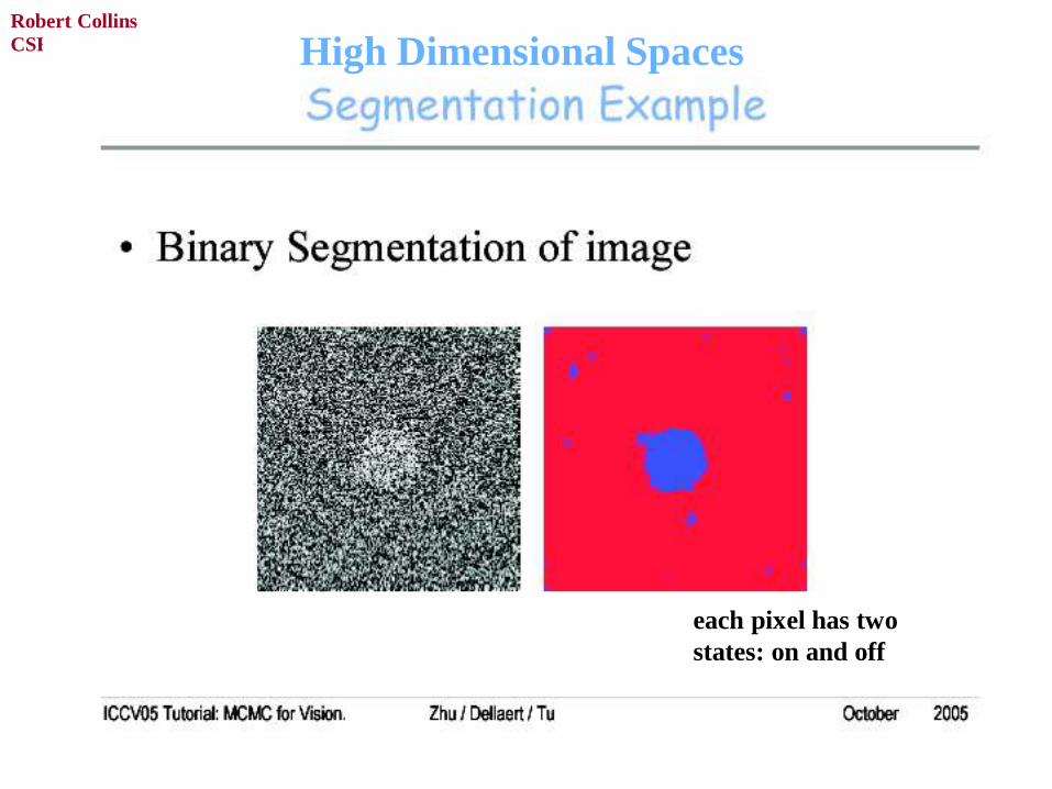
High Dimensional Spaces

each pixel has two

states: on and off

CSE586, PSU

Robert Collins

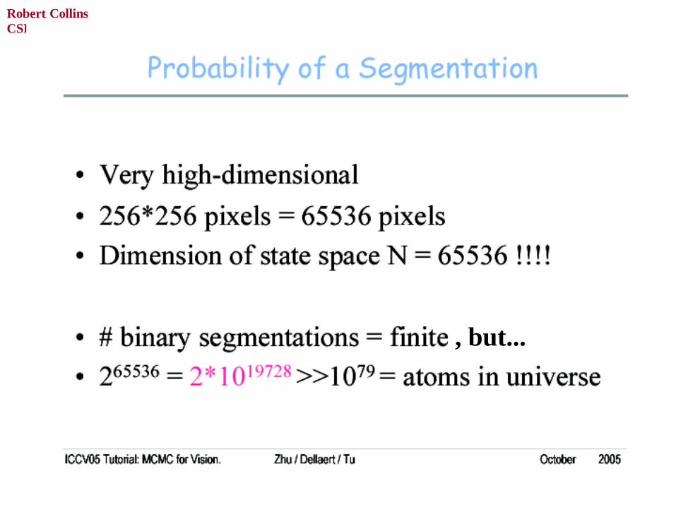
, but...

CSE586, PSU

Robert Collins

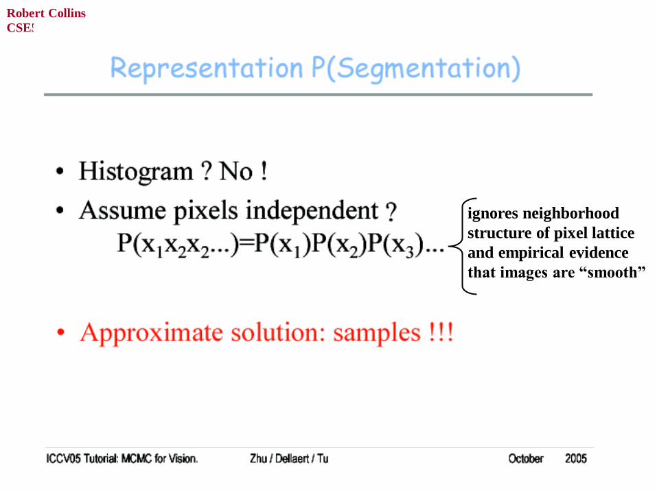
ignores neighborhood

structure of pixel lattice

and empirical evidence

that images are “smooth”

CSE586, PSU

Robert Collins

CSE586, PSU

Robert Collins

Recall: Markov Chains

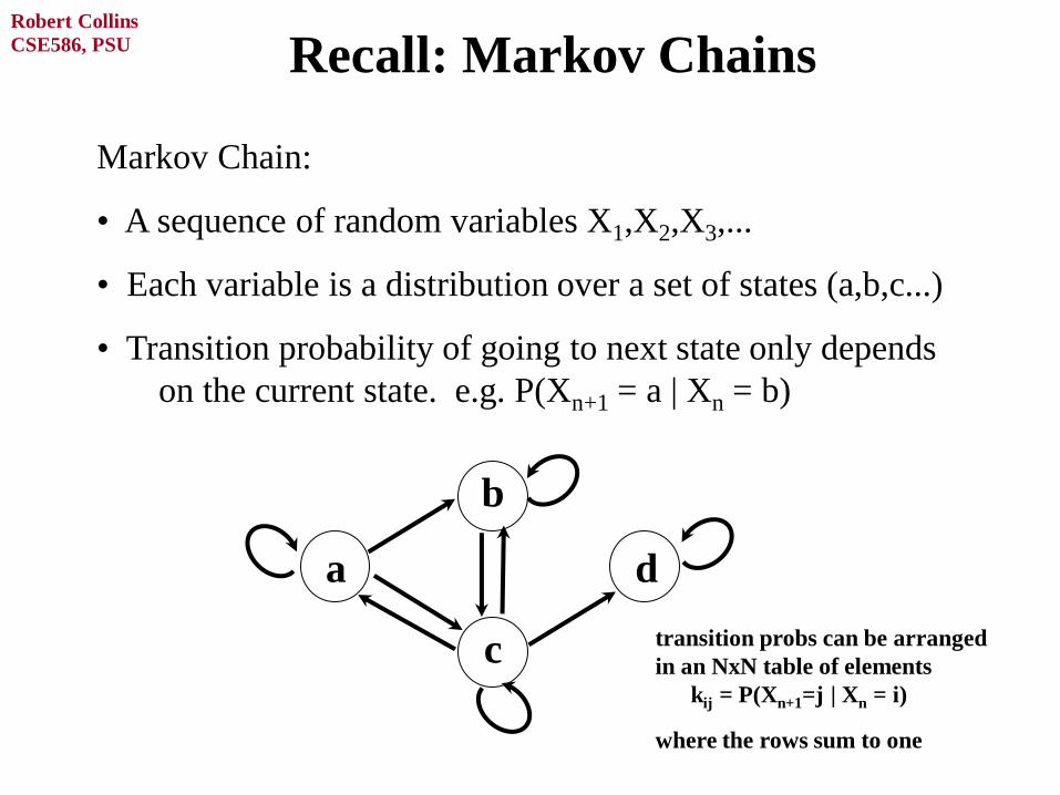
Markov Chain:

• A sequence of random variables X1,X2,X3,...

• Each variable is a distribution over a set of states (a,b,c...)

• Transition probability of going to next state only depends

on the current state. e.g. P(Xn+1 = a | Xn = b)

a

b

c

d

transition probs can be arranged

in an NxN table of elements

kij = P(Xn+1=j | Xn = i)

where the rows sum to one

CSE586, PSU

Robert Collins

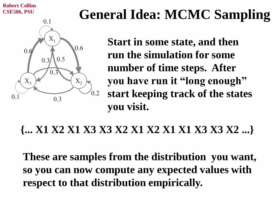
General Idea: MCMC Sampling

Start in some state, and then

run the simulation for some

number of time steps. After

you have run it “long enough”

start keeping track of the states

you visit.

{... X1 X2 X1 X3 X3 X2 X1 X2 X1 X1 X3 X3 X2 ...}

These are samples from the distribution you want,

so you can now compute any expected values with

respect to that distribution empirically.

CSE586, PSU

Robert Collins

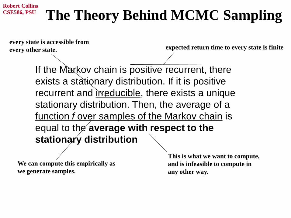
The Theory Behind MCMC Sampling

If the Markov chain is positive recurrent, there

exists a stationary distribution. If it is positive

recurrent and irreducible, there exists a unique

stationary distribution. Then, the average of a

function f over samples of the Markov chain is

equal to the average with respect to the

stationary distribution

expected return time to every state is finite every state is accessible from

every other state.

We can compute this empirically as

we generate samples.

This is what we want to compute,

and is infeasible to compute in

any other way.

CSE586, PSU

Robert Collins

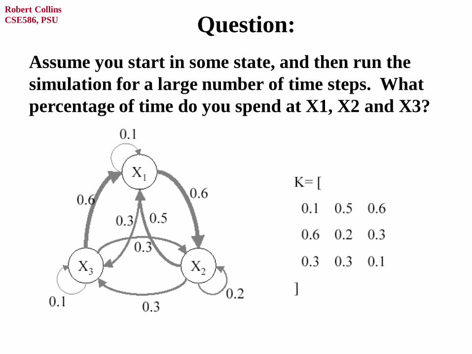
K= transpose of transition

prob table {k ij} (cols sum

to one. We do this for

computational convenience

(next slide)

CSE586, PSU

Robert Collins

Question:

Assume you start in some state, and then run the

simulation for a large number of time steps. What

percentage of time do you spend at X1, X2 and X3?

CSE586, PSU

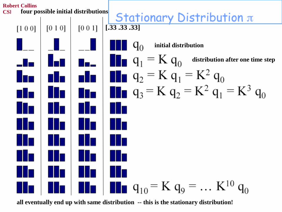
Robert Collins four possible initial distributions

[.33 .33 .33]

initial distribution

distribution after one time step

all eventually end up with same distribution -- this is the stationary distribution!

CSE586, PSU

Robert Collins

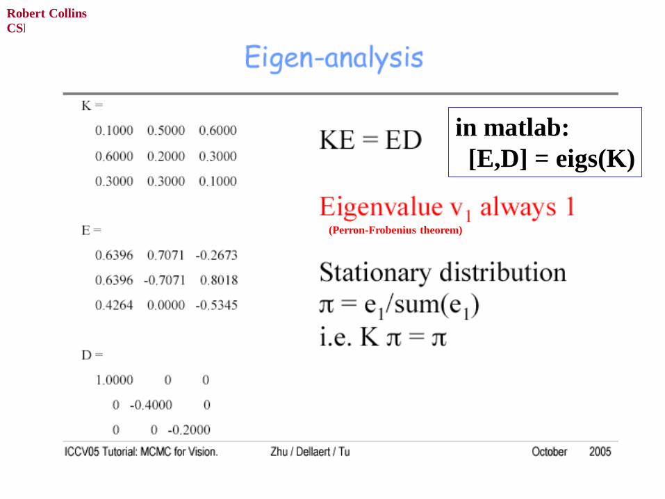
in matlab:

[E,D] = eigs(K)

(Perron-Frobenius theorem)

CSE586, PSU

Robert Collins

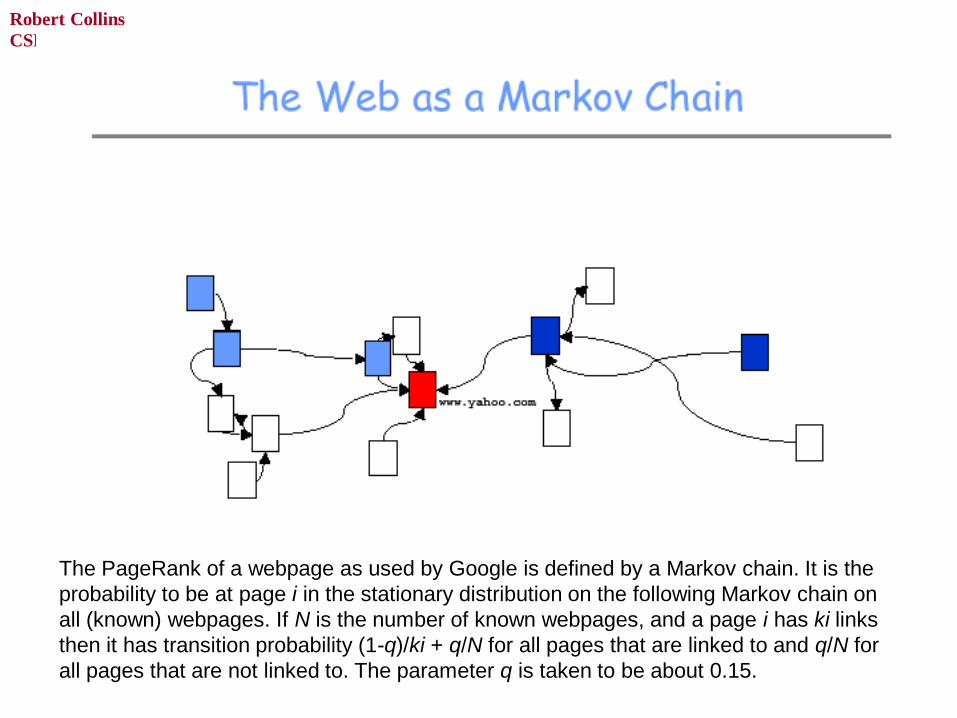
The PageRank of a webpage as used by Google is defined by a Markov chain. It is the

probability to be at page i in the stationary distribution on the following Markov chain on

all (known) webpages. If N is the number of known webpages, and a page i has ki links

then it has transition probability (1-q)/ki + q/N for all pages that are linked to and q/N for

all pages that are not linked to. The parameter q is taken to be about 0.15.

CSE586, PSU

Robert Collins

CSE586, PSU

Robert Collins

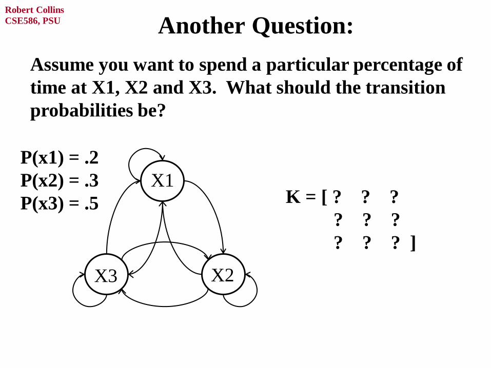
Another Question:

Assume you want to spend a particular percentage of

time at X1, X2 and X3. What should the transition

probabilities be?

X1

X2 X3

P(x1) = .2

P(x2) = .3

P(x3) = .5 K = [ ? ? ?

? ? ?

? ? ? ]

CSE586, PSU

Robert Collins

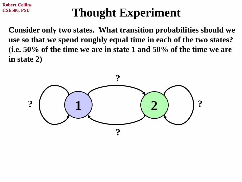
Thought Experiment

Consider only two states. What transition probabilities should we

use so that we spend roughly equal time in each of the two states?

(i.e. 50% of the time we are in state 1 and 50% of the time we are

in state 2)

1 2

?

?

? ?

CSE586, PSU

Robert Collins

Detailed Balance

• Consider a pair of configuration nodes r,s

• Want to generate them with frequency relative to their

likelihoods L(r) and L(s)

• Let q(r,s) be relative frequency of proposing configuration

s when the current state is r (and vice versa)

r

s

L(r)

L(s)

q(r,s)

q(s,r)

A sufficient condition to generate r,s

with the desired frequency is

L(r) q(r,s) = L(s) q(s,r)

“detailed balance”

CSE586, PSU

Robert Collins

Detailed Balance

• In practice, you just propose some transition probabilities.

• They typically will NOT satisfy detailed balance (unless

you are extremely lucky).

• Instead, you “fix them” by introducing a computational

fudge factor

r

s

L(r)

L(s)

a * q(r,s)

Detailed balance:

a* L(r) q(r,s) = L(s) q(s,r)

Solve for a:

a = L(s) q(s,r)

L(r) q(r,s)

q(s,r)

CSE586, PSU

Robert Collins

diff with rejection sampling: instead of

throwing away rejections, you replicate

them into next time step.

Note: you can just make up

transition probability q

on-the-fly, using whatever

criteria you wish.

CSE586, PSU

Robert Collins

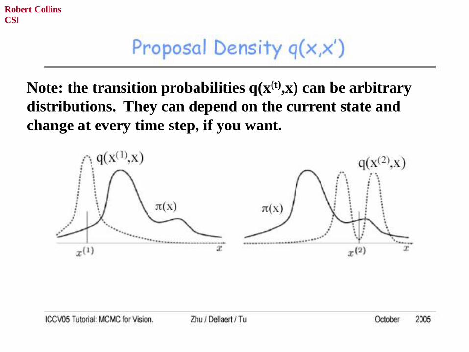
Note: the transition probabilities q(x(t),x) can be arbitrary

distributions. They can depend on the current state and

change at every time step, if you want.

CSE586, PSU

Robert Collins

Metropolis Hastings Example

X1

X2 X3

P(x1) = .2

P(x2) = .3

P(x3) = .5

Proposal distribution

q(xi, (xi-1)mod3 ) = .4

q(xi, (xi+1)mod3) = .6

Matlab demo

CSE586, PSU

Robert Collins

Variants of MCMC

• there are many variations on this general

approach, some derived as special cases of

the Metropolis-Hastings algorithm

CSE586, PSU

Robert Collins

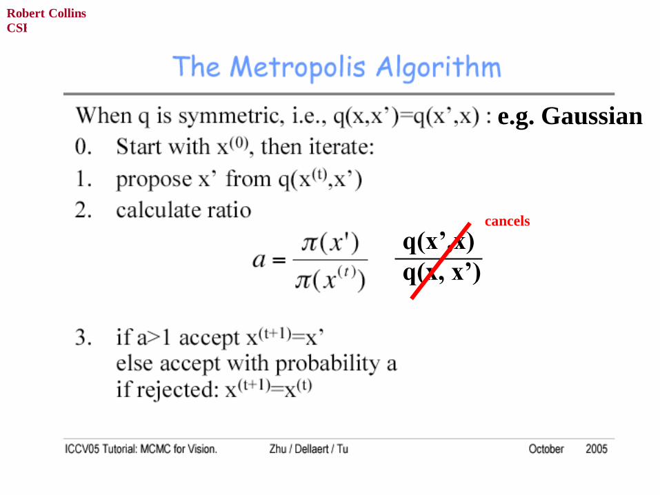
q(x’,x)

q(x, x’)

cancels

e.g. Gaussian

CSE586, PSU

Robert Collins

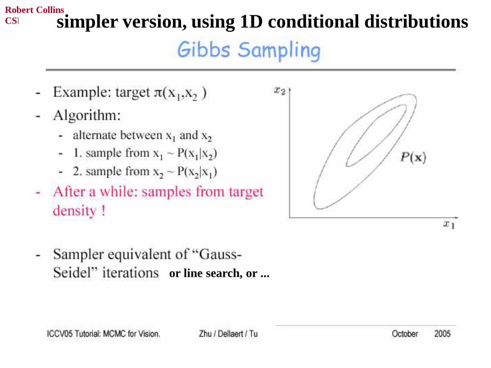
simpler version, using 1D conditional distributions

or line search, or ...

CSE586, PSU

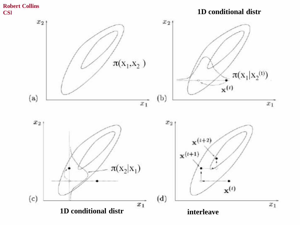
Robert Collins 1D conditional distr

1D conditional distr interleave

CSE586, PSU

Robert Collins

Simulated Annealing

• introduce a “temperature” term that makes it more

likely to accept proposals early on. This leads to

more aggressive exploration of the state space.

• Gradually reduce the temperature, causing the

process to spend more time exploring high

likelihood states.

• Rather than remember all states visited, keep track

of the best state you’ve seen so far. This is a

method that attempts to find the global max

(MAP) state.

CSE586, PSU

Robert Collins

Trans-dimensional MCMC

• Exploring alternative state spaces of differing

dimensions (example, when doing EM, also try to

estimate number of clusters along with parameters

of each cluster).

• Green’s reversible-jump approach (RJMCMC)

gives a general template for exploring and

comparing states of differing dimension.