Embed Size (px)
Citation preview

Markov Chain Models(Slides courtesy of Dr. Mark Craven)
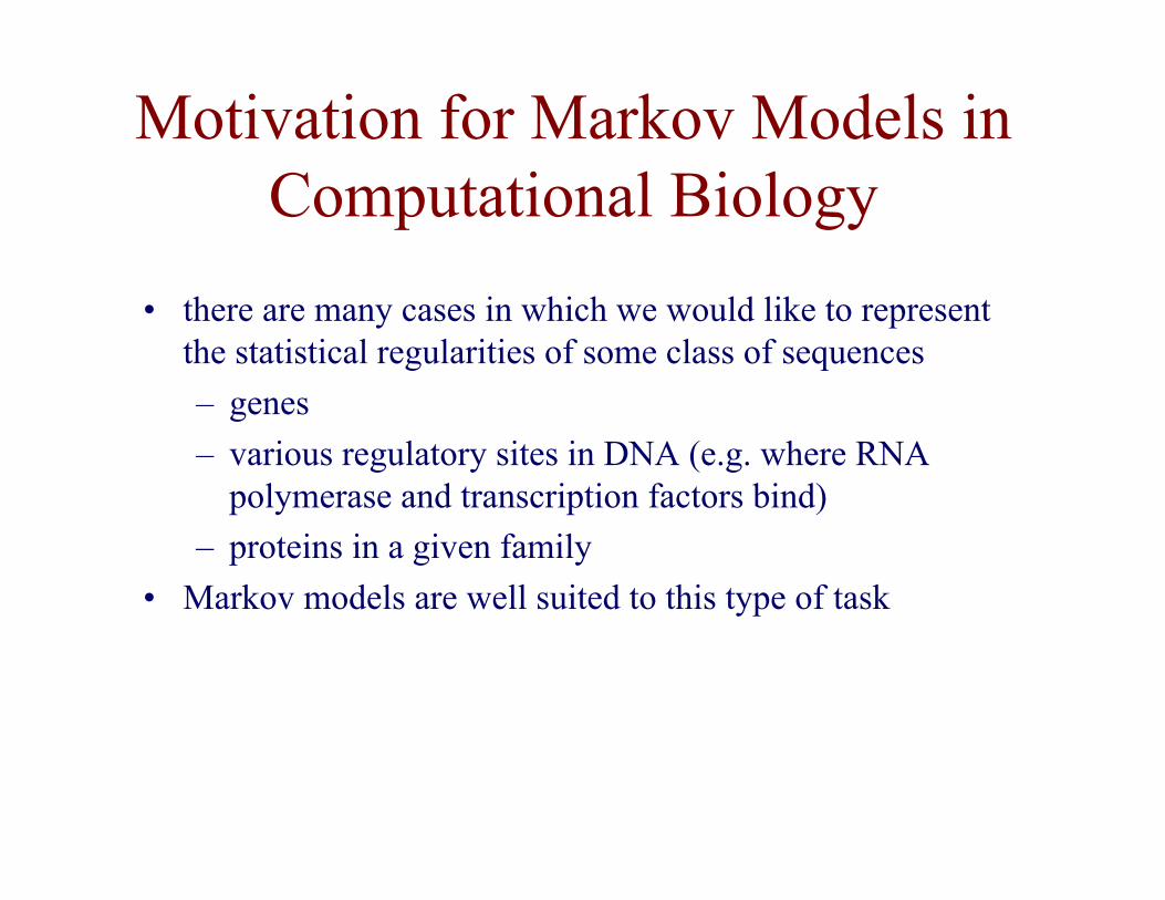
Motivation for Markov Models inComputational Biology
• there are many cases in which we would like to representthe statistical regularities of some class of sequences
– genes
– various regulatory sites in DNA (e.g. where RNApolymerase and transcription factors bind)
– proteins in a given family
• Markov models are well suited to this type of task
.34.16
.38
.12
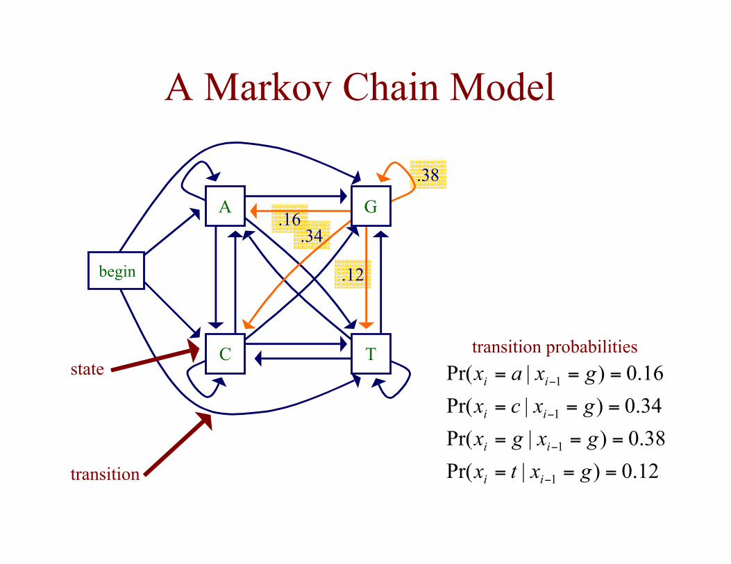
transition probabilities
12.0)|Pr(
38.0)|Pr(
34.0)|Pr(
16.0)|Pr(
1
1
1
1
===
===
===
===
−
−
−
−
gxtx
gxgx
gxcx
gxax
ii
ii
ii
ii
A Markov Chain Model
A
TC
G
begin
state
transition
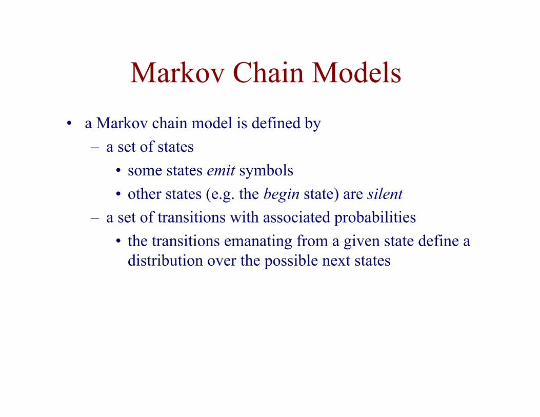
Markov Chain Models
• a Markov chain model is defined by
– a set of states
• some states emit symbols
• other states (e.g. the begin state) are silent
– a set of transitions with associated probabilities
• the transitions emanating from a given state define adistribution over the possible next states
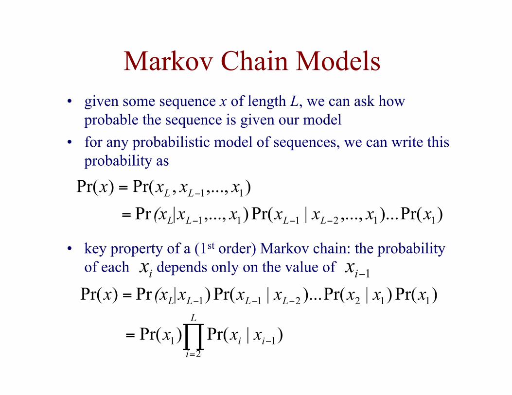
Markov Chain Models• given some sequence x of length L, we can ask how
probable the sequence is given our model
• for any probabilistic model of sequences, we can write thisprobability as
)Pr()...,...,|Pr(),...,Pr
),...,,Pr()Pr(
112111
11
xxxxx|x(x
xxxx
LLLL
LL
−−−
−
=
=
• key property of a (1st order) Markov chain: the probabilityof each depends only on the value of
)|Pr()Pr(
)Pr()|Pr()...|Pr()Pr )Pr(
12
1
112211
−=
−−−
∏=
=
i
L
ii
LLLL
xxx
xxxxx|x(xxix 1−ix
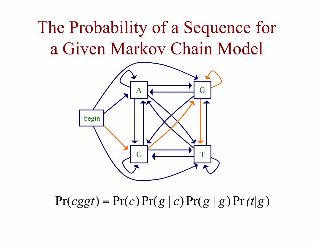
The Probability of a Sequence fora Given Markov Chain Model
A
TC
G
begin
)Pr)|Pr()|Pr()Pr( )Pr( (t|gggcgccggt =
Markov Chain Models
begin end
A
TC
G
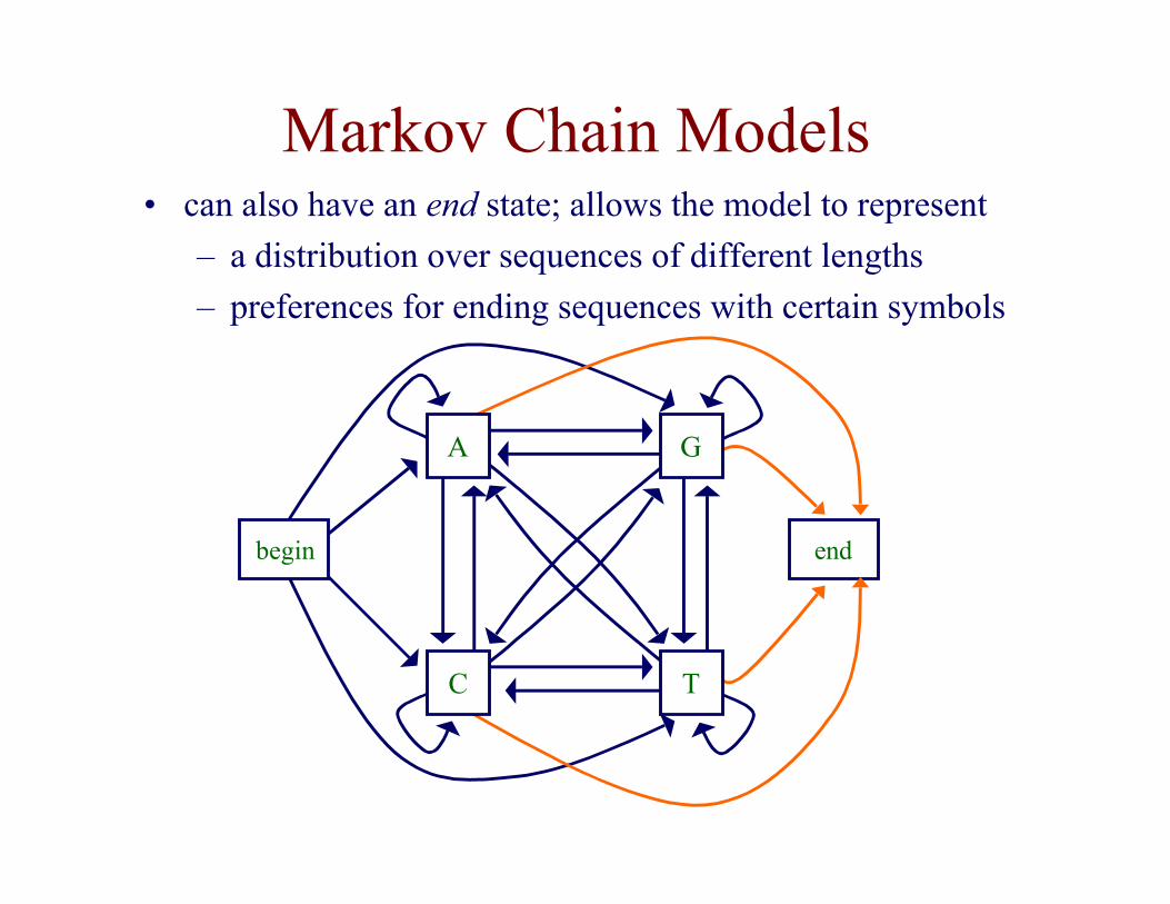
• can also have an end state; allows the model to represent
– a distribution over sequences of different lengths
– preferences for ending sequences with certain symbols
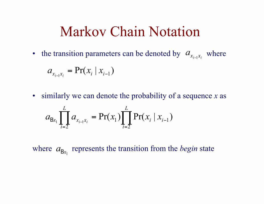
Markov Chain Notation• the transition parameters can be denoted by where
• similarly we can denote the probability of a sequence x as
where represents the transition from the begin state
)|Pr()Pr( 12
12
11 −==∏∏ =
− i
L
ii
L
ixxx xxxaaiiB
)|Pr( 11 −=− iixx xxa
ii
ii xxa 1−
1xaB
Example Application
• CpG islands
– CG dinucleotides are rarer in eukaryotic genomes thanexpected given the marginal probabilities of C and G
– but the regions upstream of genes are richer in CGdinucleotides than elsewhere – CpG islands
– useful evidence for finding genes
• could predict CpG islands with Markov chains
– one to represent CpG islands
– one to represent the rest of the genome
Estimating the Model Parameters
• given some data (e.g. a set of sequences from CpGislands), how can we determine the probability parametersof our model?
• one approach: maximum likelihood estimation
– given a set of data D
– set the parameters to maximize
– i.e. make the data D look likely under the model
)|Pr( θDθ
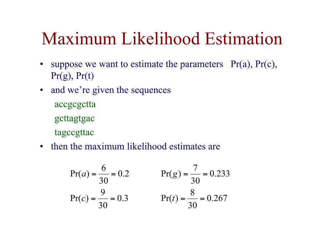
Maximum Likelihood Estimation• suppose we want to estimate the parameters Pr(a), Pr(c),
Pr(g), Pr(t)
• and we’re given the sequences
accgcgctta
gcttagtgac
tagccgttac
• then the maximum likelihood estimates are
267.030
8)Pr(
233.030
7)Pr(
==
==
t
g
3.030
9)Pr(
2.030
6)Pr(
==
==
c
a
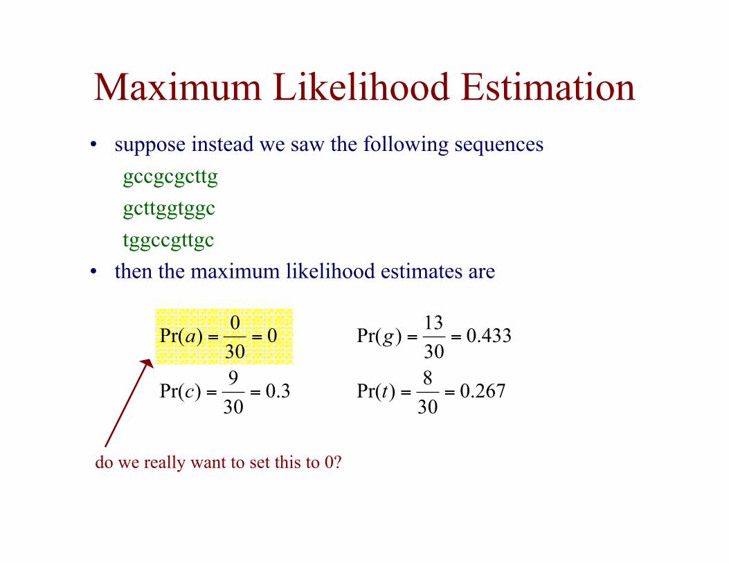
Maximum Likelihood Estimation• suppose instead we saw the following sequences
gccgcgcttg
gcttggtggc
tggccgttgc
• then the maximum likelihood estimates are
267.030
8)Pr(
433.030
13)Pr(
==
==
t
g
3.030
9)Pr(
030
0)Pr(
==
==
c
a
do we really want to set this to 0?
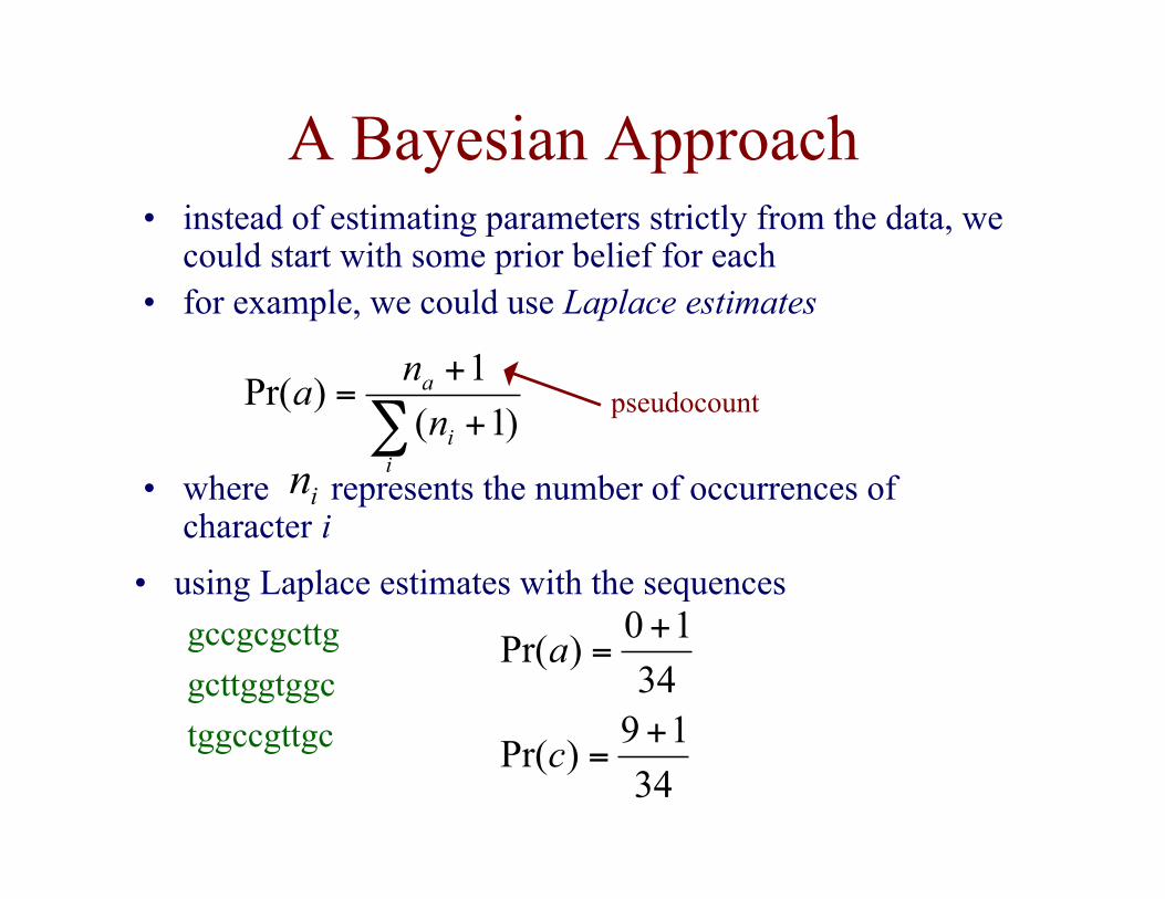
A Bayesian Approach• instead of estimating parameters strictly from the data, we
could start with some prior belief for each• for example, we could use Laplace estimates
• where represents the number of occurrences ofcharacter i
∑ +
+=
ii
a
n
na
)1(
1)Pr(
• using Laplace estimates with the sequences
gccgcgcttg
gcttggtggc
tggccgttgc
34
19)Pr(
34
10)Pr(
+=
+=
c
a
pseudocount
in
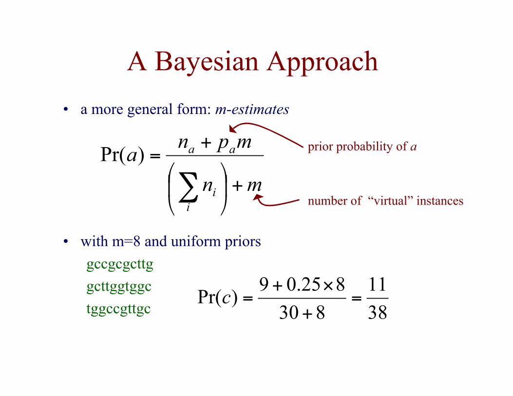
A Bayesian Approach
• a more general form: m-estimates
mn
mpna
ii
aa
+
+=
∑)Pr(
• with m=8 and uniform priors
gccgcgcttg
gcttggtggc
tggccgttgc
number of “virtual” instances
prior probability of a
38
11
830
825.09)Pr( =
+
×+=c
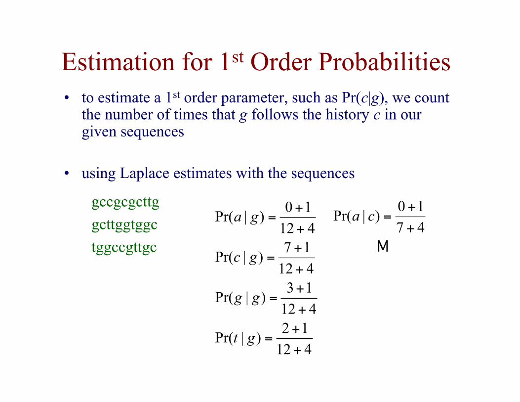
Estimation for 1st Order Probabilities• to estimate a 1st order parameter, such as Pr(c|g), we count
the number of times that g follows the history c in ourgiven sequences
• using Laplace estimates with the sequences
gccgcgcttg
gcttggtggc
tggccgttgc
412
12)|Pr(
412
13)|Pr(
412
17)|Pr(
412
10)|Pr(
+
+=
+
+=
+
+=
+
+=
gt
gg
gc
ga
M47
10)|Pr(
+
+=ca

Markov Chain Models
begin end
A
TC
G
• can also have an end state; allows the model to represent
– a distribution over sequences of different lengths
– preferences for ending sequences with certain symbols
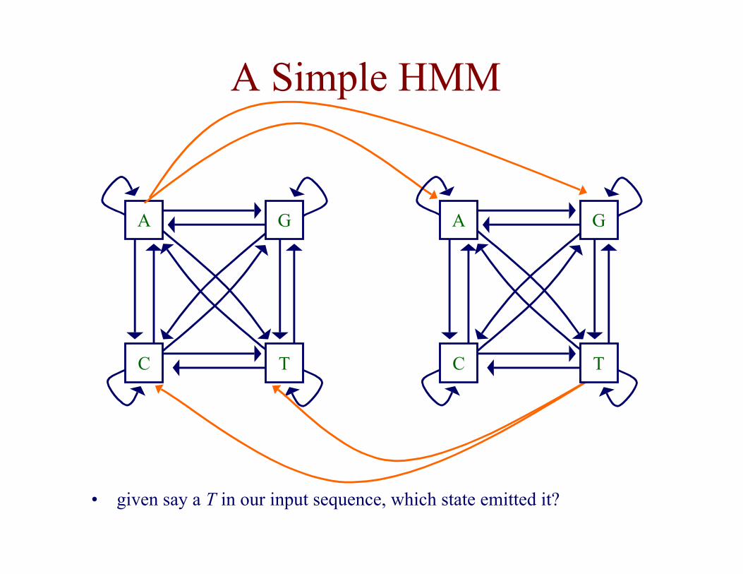
A Simple HMM
A
TC
G A
TC
G
• given say a T in our input sequence, which state emitted it?
Hidden State
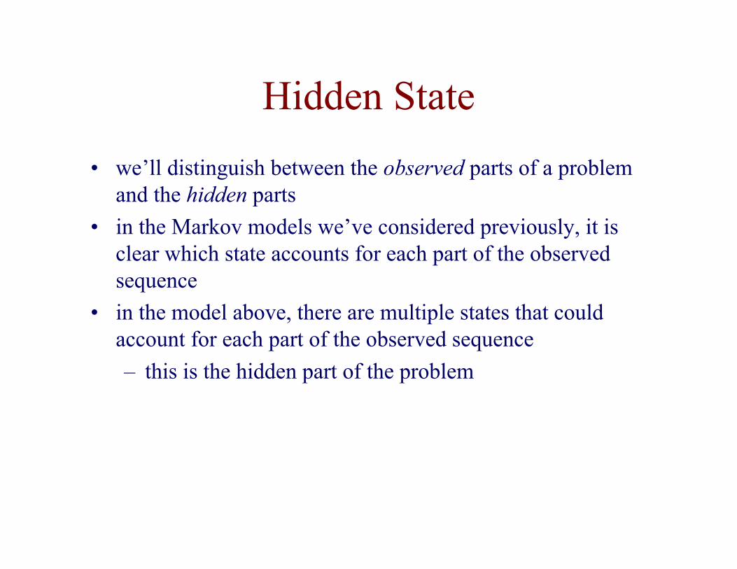
• we’ll distinguish between the observed parts of a problemand the hidden parts
• in the Markov models we’ve considered previously, it isclear which state accounts for each part of the observedsequence
• in the model above, there are multiple states that couldaccount for each part of the observed sequence
– this is the hidden part of the problem
The Parameters of an HMM
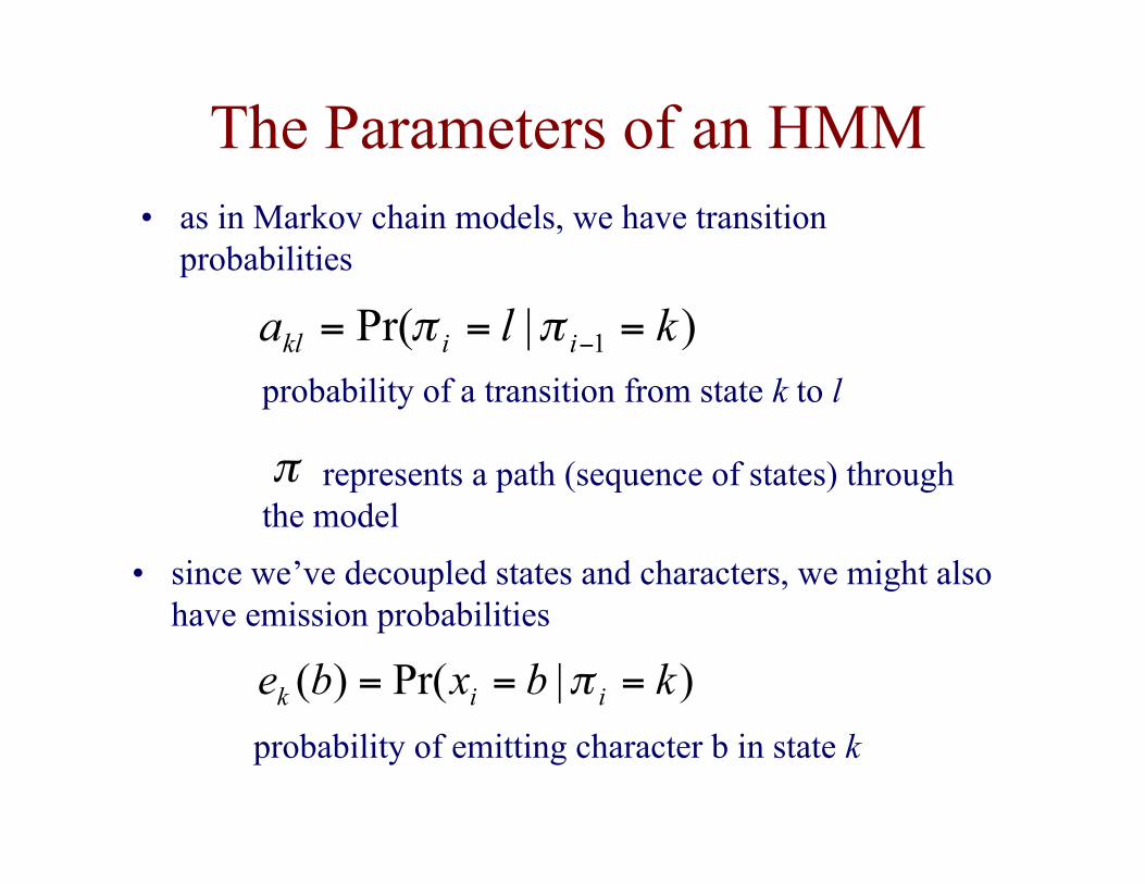
• since we’ve decoupled states and characters, we might alsohave emission probabilities
)|Pr()( kbxbe iik === π
)|Pr( 1 kla iikl === −ππ
probability of emitting character b in state k
probability of a transition from state k to l
represents a path (sequence of states) throughthe model
• as in Markov chain models, we have transitionprobabilities
π
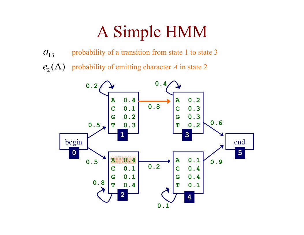
A Simple HMM
0.8
)A(2e13a
probability of emitting character A in state 2
probability of a transition from state 1 to state 3
0.4
A 0.4C 0.1G 0.2T 0.3
A 0.1C 0.4G 0.4T 0.1
A 0.2C 0.3G 0.3T 0.2
begin end
0.5
0.5
0.2
0.8
0.6
0.1
0.90.2
0 5
4
3
2
1
A 0.4C 0.1G 0.1T 0.4
Three Important Questions
• How likely is a given sequence?
the Forward algorithm
• What is the most probable “path” for generating a givensequence?
the Viterbi algorithm
• How can we learn the HMM parameters given a set ofsequences?
the Forward-Backward (Baum-Welch) algorithm
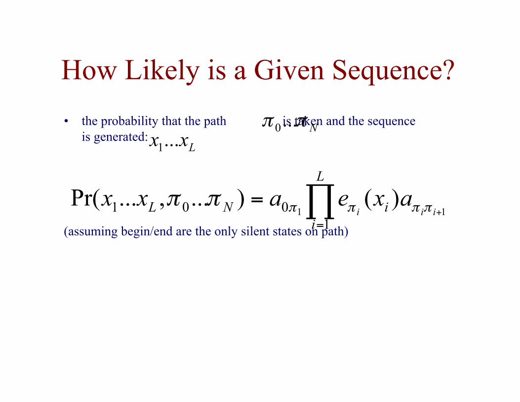
How Likely is a Given Sequence?
• the probability that the path is taken and the sequenceis generated:
(assuming begin/end are the only silent states on path)
∏=
+=
L
iiNL iiiaxeaxx
1001 11
)()...,...Pr( ππππππ
Lxx ...1
Nππ ...0
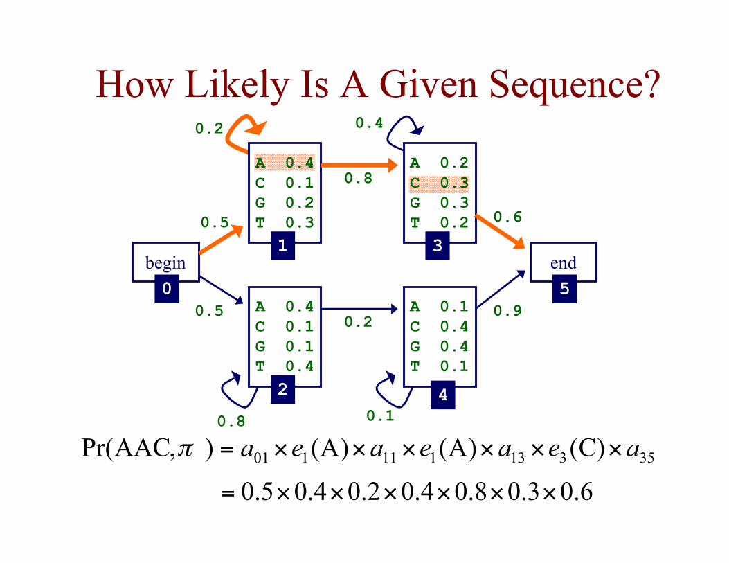
How Likely Is A Given Sequence?
A 0.1C 0.4G 0.4T 0.1
A 0.4C 0.1G 0.1T 0.4
begin end
0.5
0.5
0.2
0.8
0.4
0.6
0.1
0.90.2
0.8
0 5
4
3
2
1
6.03.08.04.02.04.05.0
)C()A()A(),AACPr( 35313111101
××××××=
××××××= aeaeaeaπ
A 0.4C 0.1G 0.2T 0.3
A 0.2C 0.3G 0.3T 0.2
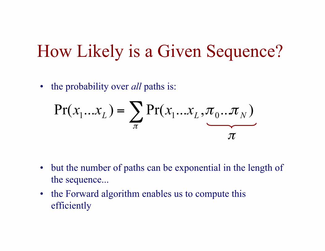
How Likely is a Given Sequence?
• the probability over all paths is:
)...,...Pr( )...Pr( 011 ∑=π
ππ NLL xxxx
• but the number of paths can be exponential in the length ofthe sequence...
• the Forward algorithm enables us to compute thisefficiently
π
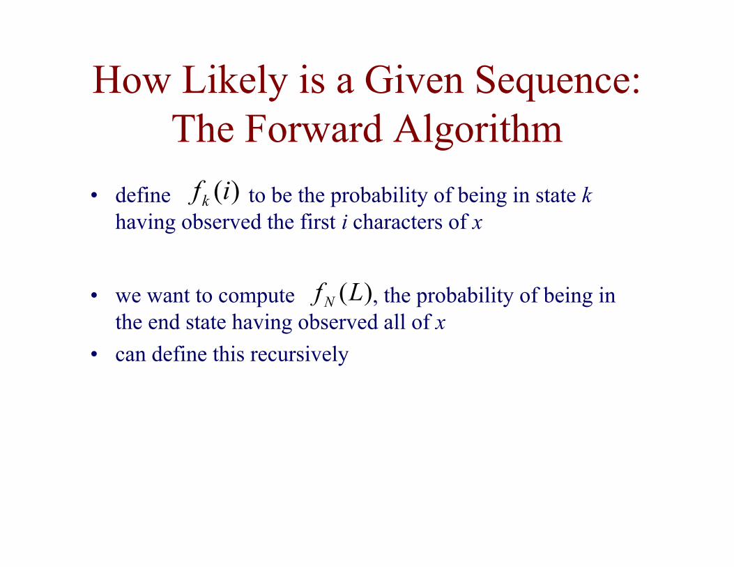
How Likely is a Given Sequence:The Forward Algorithm
• define to be the probability of being in state khaving observed the first i characters of x
)(ifk
• we want to compute , the probability of being inthe end state having observed all of x
• can define this recursively
)(LfN
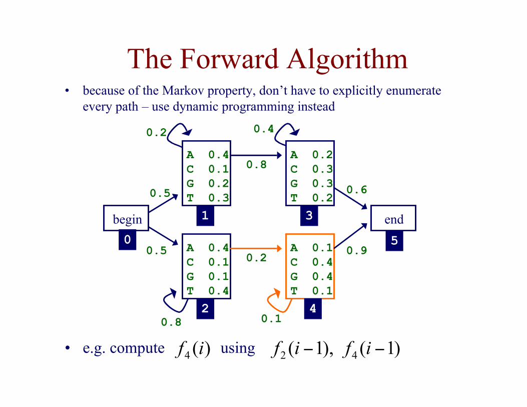
The Forward Algorithm• because of the Markov property, don’t have to explicitly enumerate
every path – use dynamic programming instead
)(4 if )1( ),1( 42 −− ifif• e.g. compute using
A 0.4C 0.1G 0.2T 0.3
A 0.1C 0.4G 0.4T 0.1
A 0.4C 0.1G 0.1T 0.4
A 0.2C 0.3G 0.3T 0.2
begin end
0.5
0.5
0.2
0.8
0.4
0.6
0.1
0.90.2
0.8
0 5
4
3
2
1
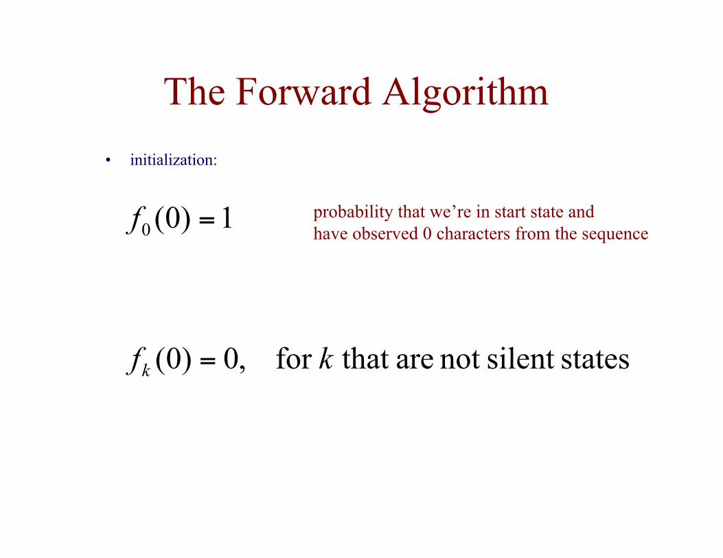
The Forward Algorithm
• initialization:
1)0(0 =f
statessilent not are that for ,0)0( kfk =
probability that we’re in start state andhave observed 0 characters from the sequence
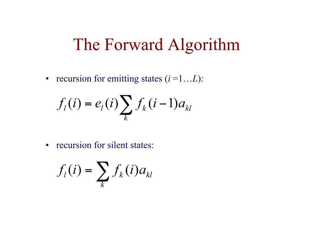
The Forward Algorithm
∑=k
klkl aifif )()(
• recursion for silent states:
∑ −=k
klkll aifieif )1()()(
• recursion for emitting states (i =1…L):
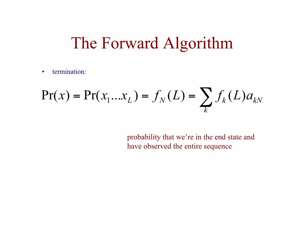
The Forward Algorithm
• termination:
∑===k
kNkNL aLfLfxxx )()()...Pr()Pr( 1
probability that we’re in the end state andhave observed the entire sequence
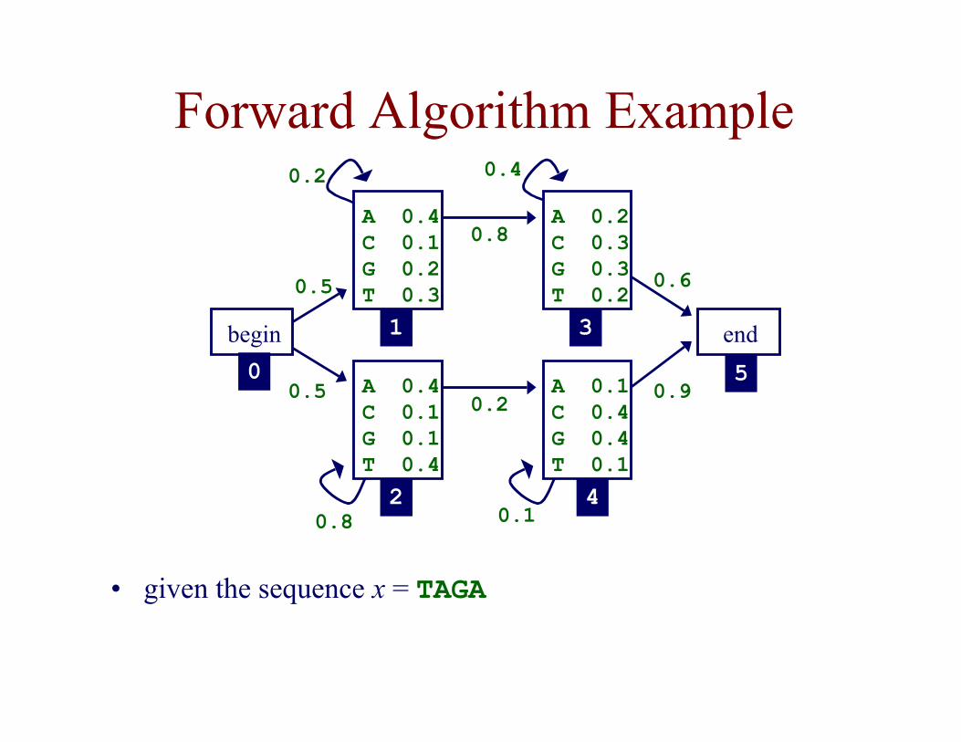
Forward Algorithm Example
A 0.4C 0.1G 0.2T 0.3
A 0.1C 0.4G 0.4T 0.1
A 0.4C 0.1G 0.1T 0.4
A 0.2C 0.3G 0.3T 0.2
begin end
0.5
0.5
0.2
0.8
0.4
0.6
0.1
0.90.2
0.8
0 5
4
3
2
1
• given the sequence x = TAGA
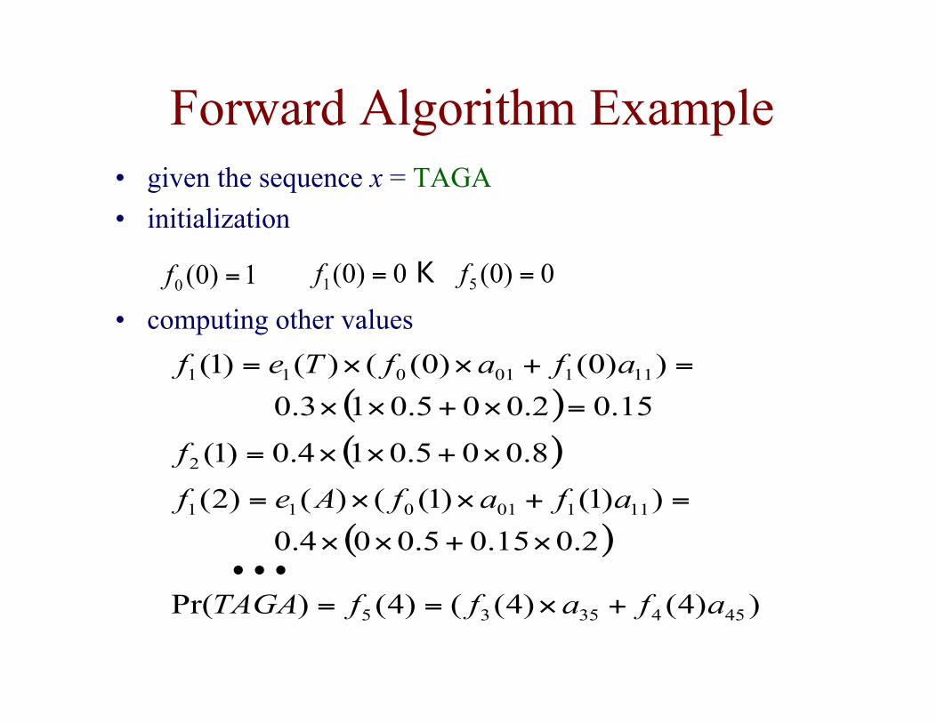
Forward Algorithm Example
1)0(0 =f 0)0( 0)0( 51 == ff K
• given the sequence x = TAGA
• initialization
• computing other values
( ) 15.02.005.013.0
))0()0(()()1( 11101011
=×+××
=+××= afafTef
...( )8.005.014.0)1(2 ×+××=f
( )2.015.05.004.0
))1()1(()()2( 11101011
×+××
=+××= afafAef
))4()4(()4()Pr( 4543535 afaffTAGA +×==
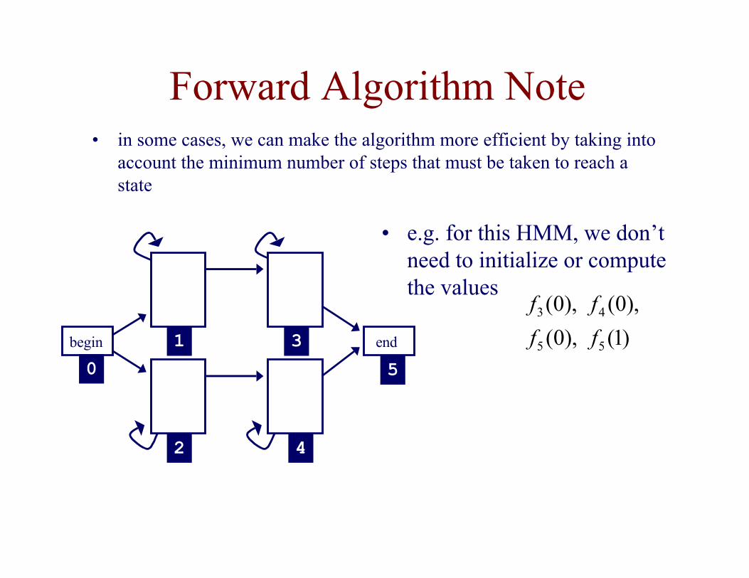
Forward Algorithm Note• in some cases, we can make the algorithm more efficient by taking into
account the minimum number of steps that must be taken to reach astate
begin end
0 5
4
3
2
1
• e.g. for this HMM, we don’tneed to initialize or computethe values
)1( ,)0(
,)0( ,)0(
55
43
ff
ff
Three Important Questions
• How likely is a given sequence?
• What is the most probable “path” for generating a givensequence?
• How can we learn the HMM parameters given a set ofsequences?
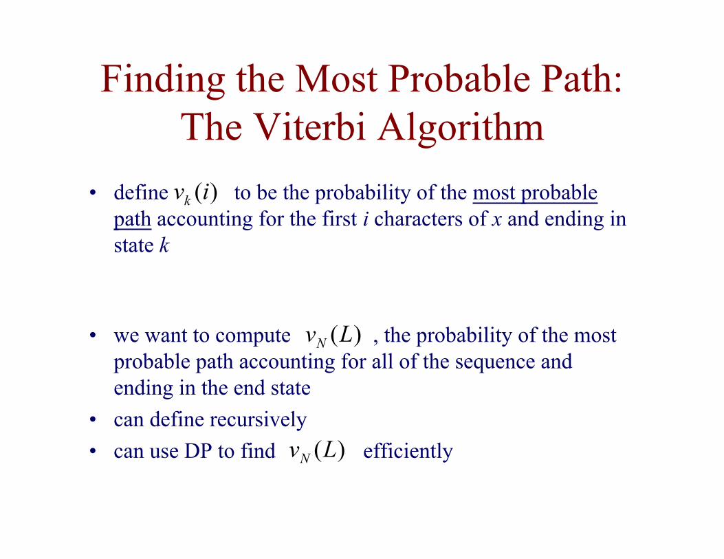
Finding the Most Probable Path:The Viterbi Algorithm
• define to be the probability of the most probablepath accounting for the first i characters of x and ending instate k
)(ivk
• we want to compute , the probability of the mostprobable path accounting for all of the sequence andending in the end state
• can define recursively
• can use DP to find efficiently
)(LvN
)(LvN
Finding the Most Probable Path:The Viterbi Algorithm
• initialization:
1)0(0 =v
statessilent not are that for ,0)0( kvk =
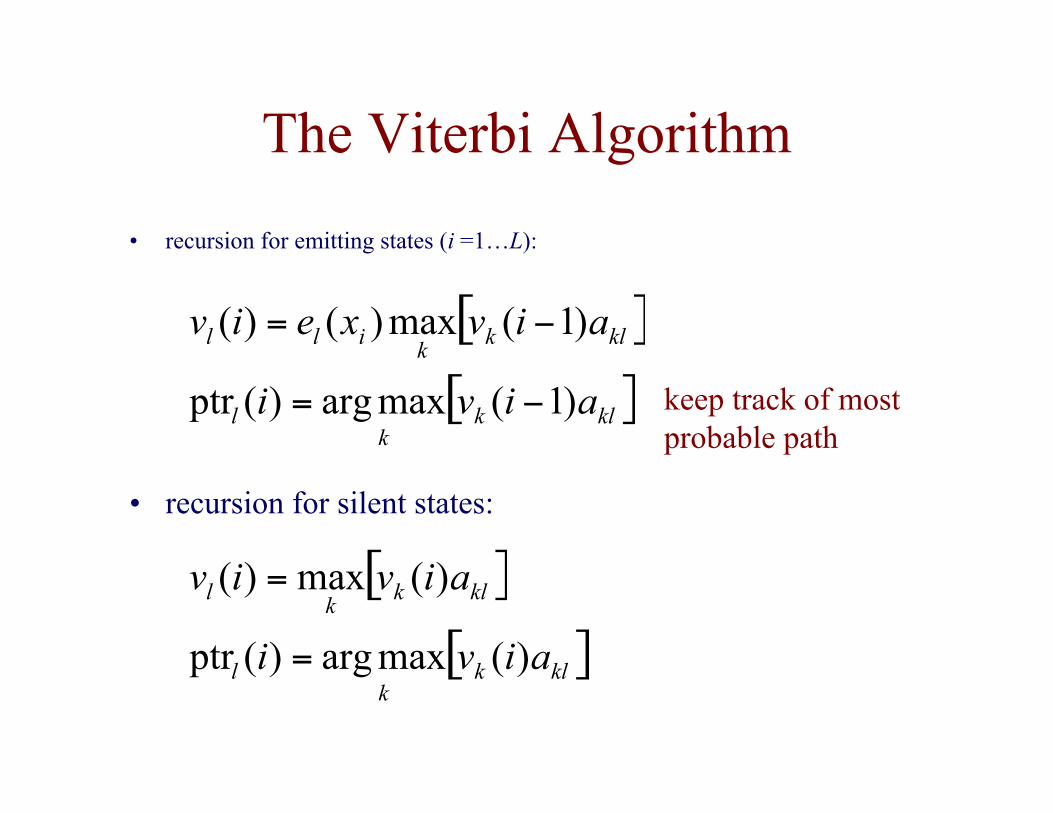
The Viterbi Algorithm
• recursion for emitting states (i =1…L):
[ ]klkk
ill aivxeiv )1(max)()( −=
[ ]klkk
l aiviv )(max)( =
• recursion for silent states:
[ ]klkk
l aivi )(maxarg)(ptr =
[ ]klkk
l aivi )1(maxarg)(ptr −= keep track of most probable path
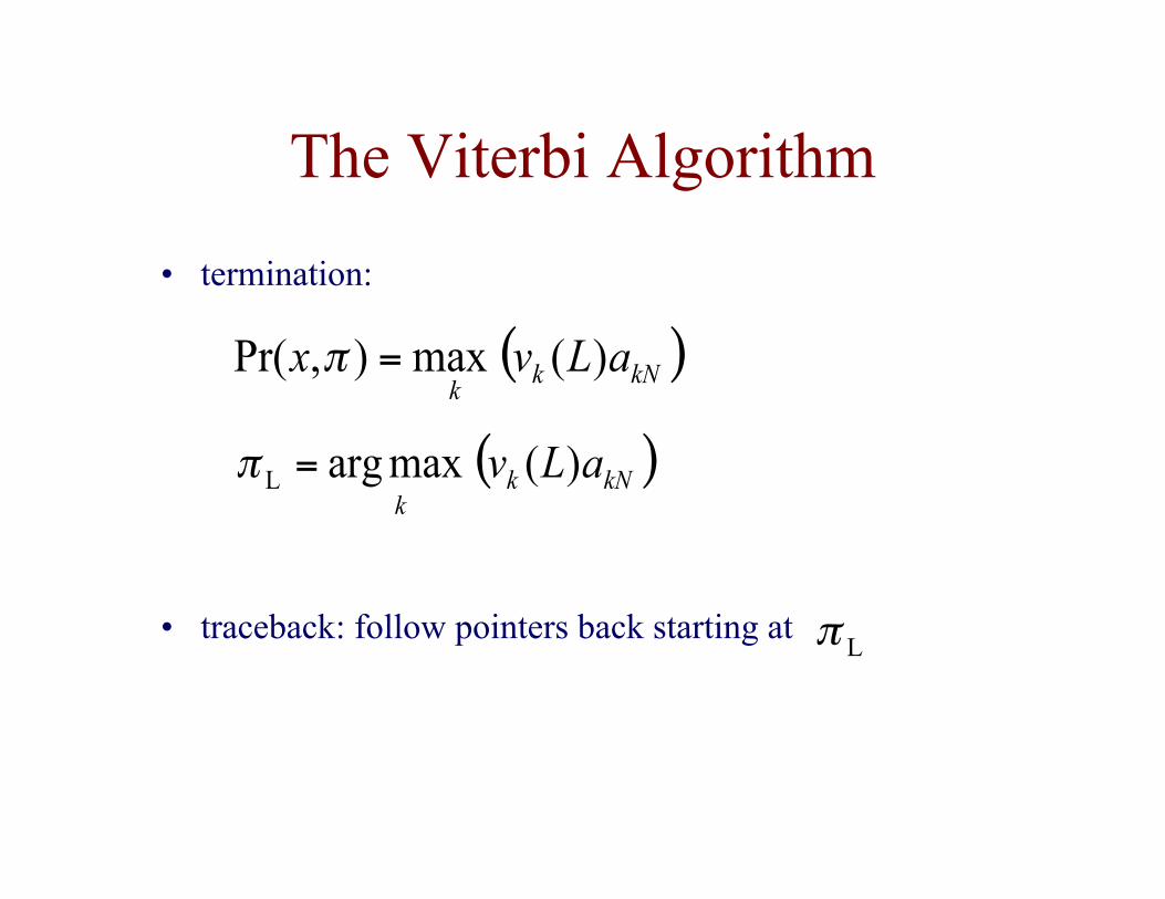
The Viterbi Algorithm
• traceback: follow pointers back starting at
• termination:
Lπ
( )kNkk
aLv )( maxargL =π
( )kNkk
aLvx )( max),Pr( =π
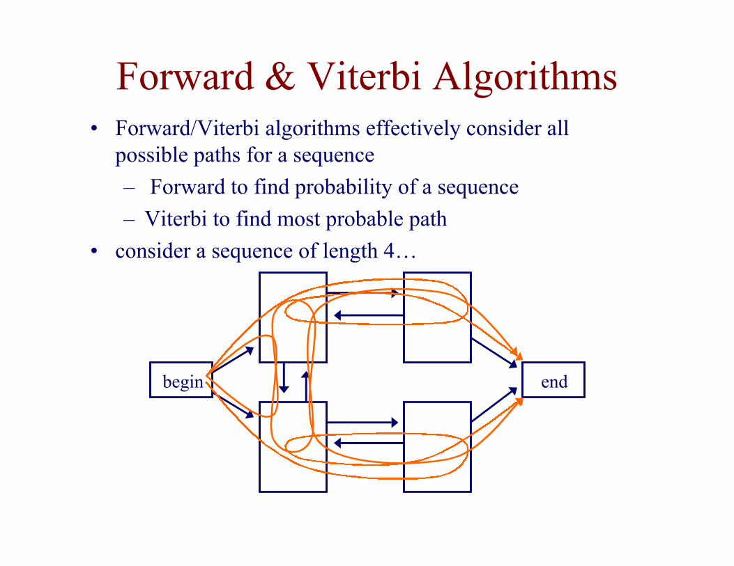
Forward & Viterbi Algorithms
begin end
• Forward/Viterbi algorithms effectively consider allpossible paths for a sequence
– Forward to find probability of a sequence
– Viterbi to find most probable path
• consider a sequence of length 4…
Three Important Questions
• How likely is a given sequence?
• What is the most probable “path” for generating a givensequence?
• How can we learn the HMM parameters given a set ofsequences?
Learning Parameters
• if we know the state path for each training sequence, learning themodel parameters is simple– no hidden state during training– count how often each parameter is used– normalize/smooth to get probabilities– process is just like it was for Markov chain models
• if we don’t know the path for each training sequence, how can wedetermine the counts?– key insight: estimate the counts by considering every path
weighted by its probability
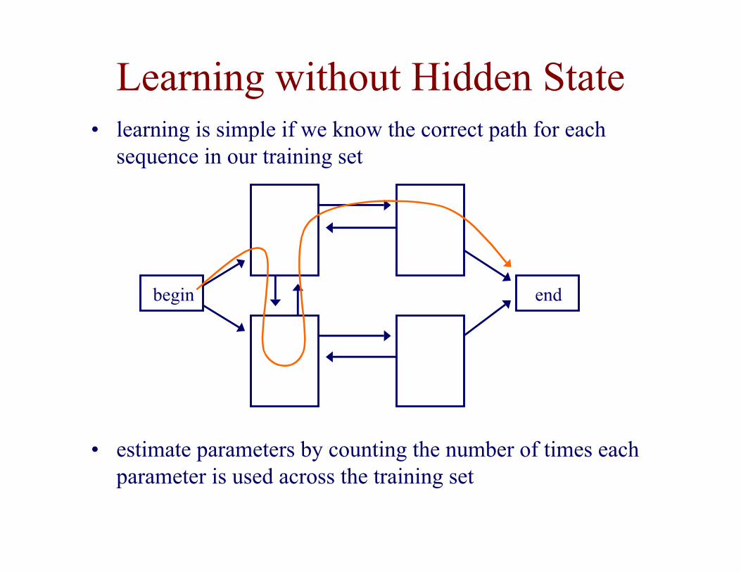
Learning without Hidden State
begin end
• learning is simple if we know the correct path for eachsequence in our training set
• estimate parameters by counting the number of times eachparameter is used across the training set
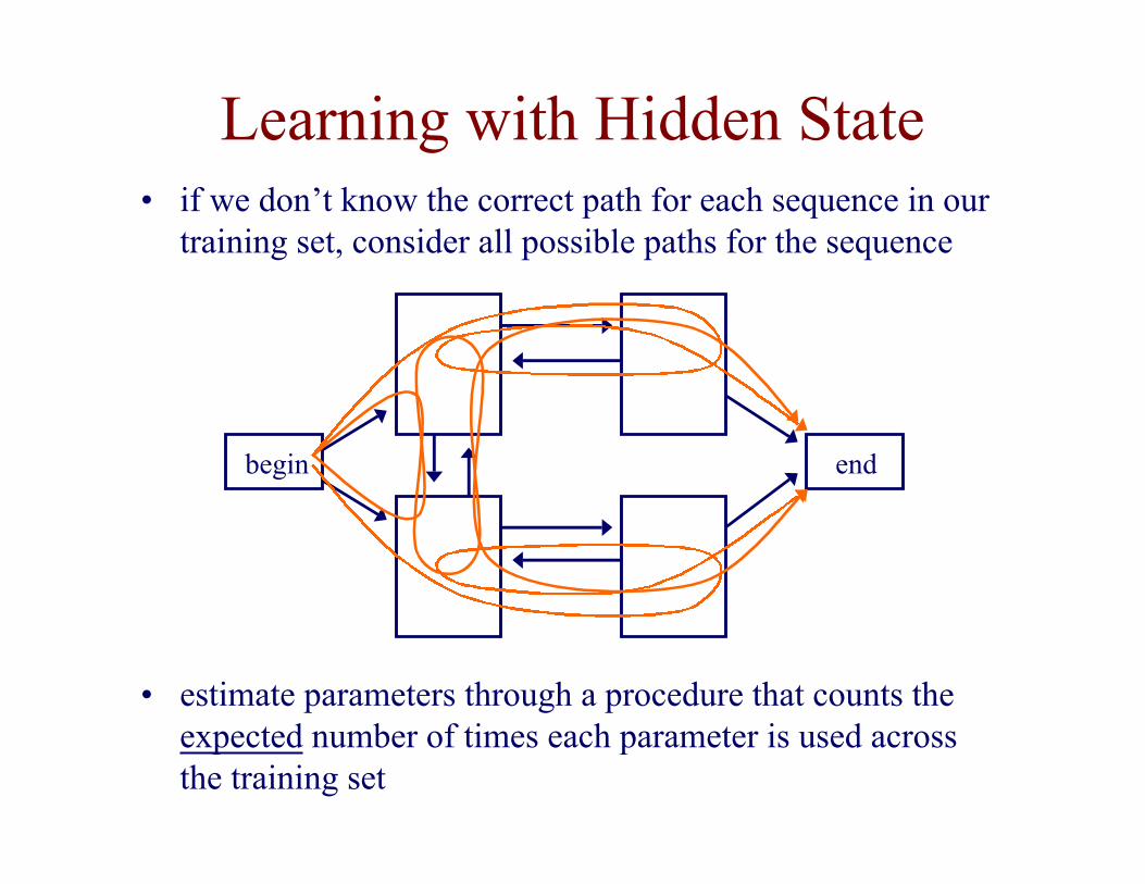
Learning with Hidden State• if we don’t know the correct path for each sequence in our
training set, consider all possible paths for the sequence
• estimate parameters through a procedure that counts theexpected number of times each parameter is used acrossthe training set
begin end
Learning Parameters:The Baum-Welch Algorithm
• a.k.a the Forward-Backward algorithm
• an Expectation Maximization (EM) algorithm
– EM is a family of algorithms for learning probabilisticmodels in problems that involve hidden state
• in this context, the hidden state is the path that bestexplains each training sequence
Learning Parameters:The Baum-Welch Algorithm
• algorithm sketch:
– initialize parameters of model
– iterate until convergence
• calculate the expected number of times eachtransition or emission is used
• adjust the parameters to maximize the likelihood ofthese expected values
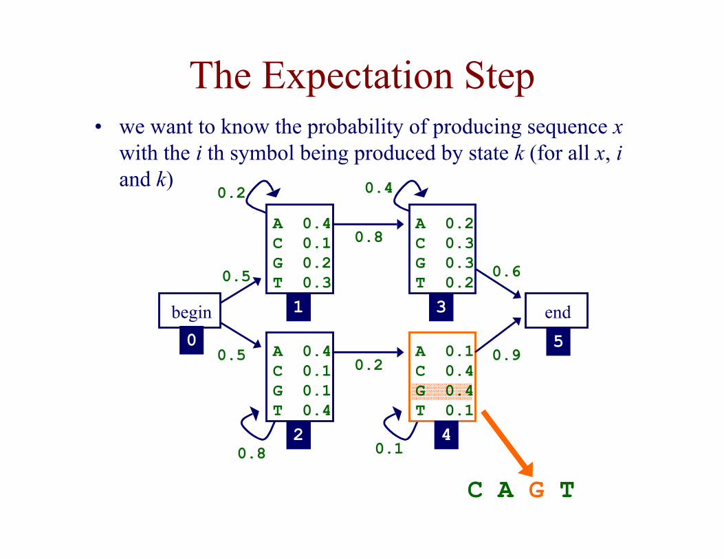
The Expectation Step• we want to know the probability of producing sequence x
with the i th symbol being produced by state k (for all x, iand k)
C A G T
A 0.4C 0.1G 0.2T 0.3
A 0.4C 0.1G 0.1T 0.4
A 0.2C 0.3G 0.3T 0.2
begin end
0.5
0.5
0.2
0.8
0.4
0.6
0.1
0.90.2
0.8
0 5
4
3
2
1
A 0.1C 0.4G 0.4T 0.1
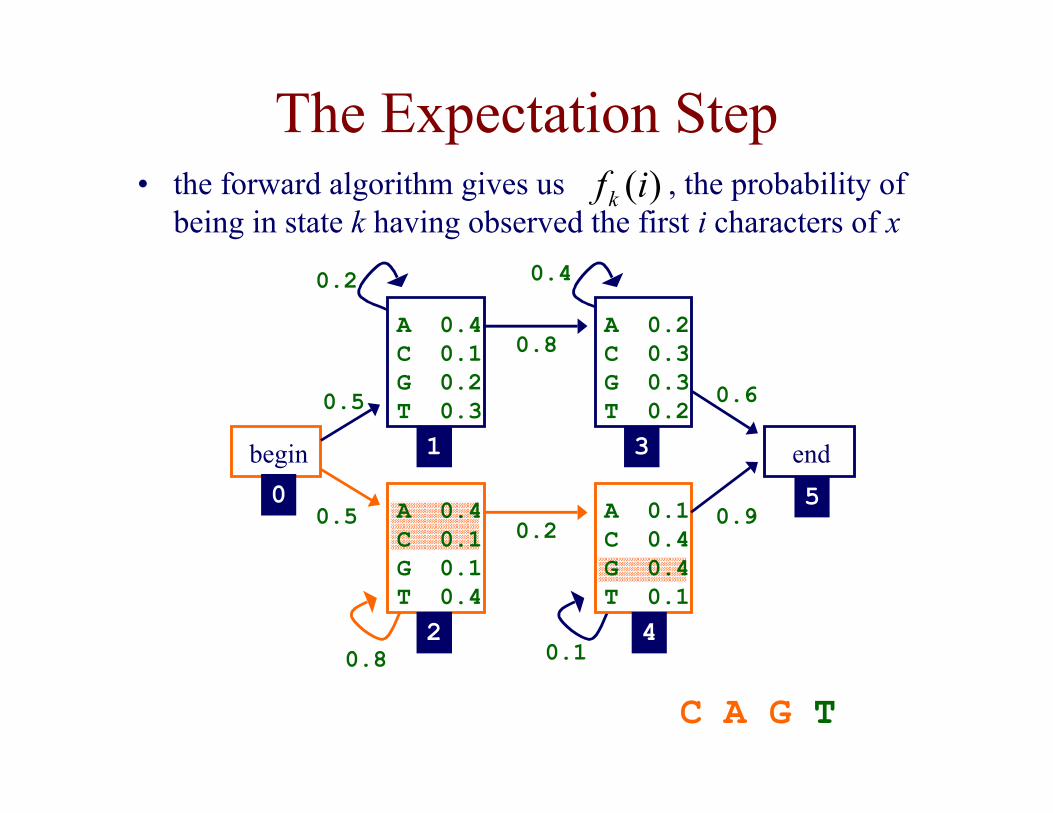
The Expectation Step• the forward algorithm gives us , the probability of
being in state k having observed the first i characters of x)(ifk
A 0.4C 0.1G 0.2T 0.3
A 0.2C 0.3G 0.3T 0.2
begin end
0.5
0.5
0.2
0.8
0.4
0.6
0.1
0.90.2
0.8
0 5
4
3
2
1
A 0.1C 0.4G 0.4T 0.1
C A G T
A 0.4C 0.1G 0.1T 0.4
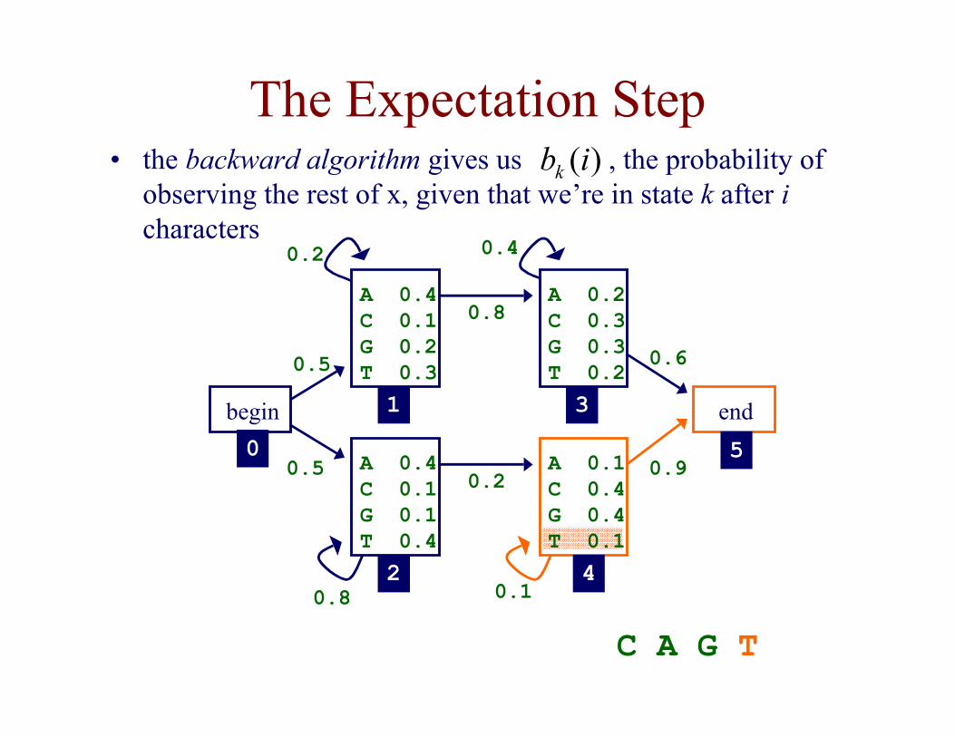
The Expectation Step• the backward algorithm gives us , the probability of
observing the rest of x, given that we’re in state k after icharacters
)(ibk
A 0.4C 0.1G 0.2T 0.3
A 0.2C 0.3G 0.3T 0.2
begin end
0.5
0.5
0.2
0.8
0.4
0.6
0.1
0.90.2
0.8
0 5
4
3
2
1
A 0.1C 0.4G 0.4T 0.1
C A G T
A 0.4C 0.1G 0.1T 0.4
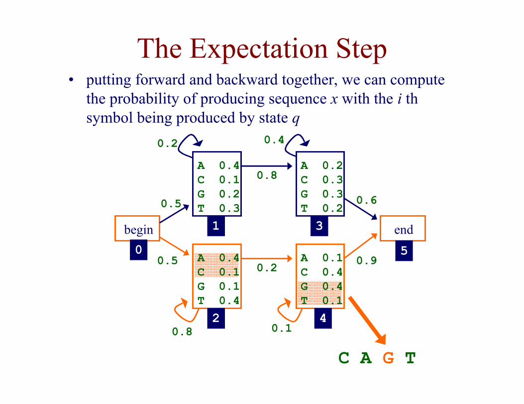
The Expectation Step• putting forward and backward together, we can compute
the probability of producing sequence x with the i thsymbol being produced by state q
A 0.4C 0.1G 0.2T 0.3
A 0.2C 0.3G 0.3T 0.2
begin end
0.5
0.5
0.2
0.8
0.4
0.6
0.1
0.90.2
0.8
0 5
4
3
2
1
C A G T
A 0.4C 0.1G 0.1T 0.4
A 0.1C 0.4G 0.4T 0.1
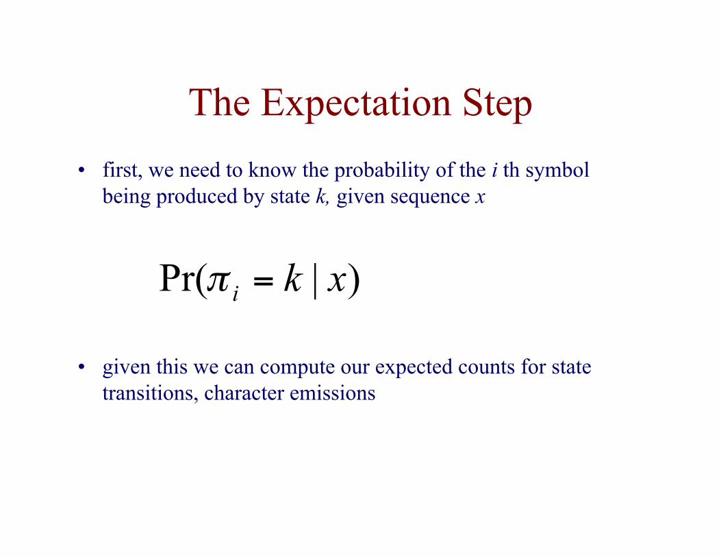
The Expectation Step
• first, we need to know the probability of the i th symbolbeing produced by state k, given sequence x
)|Pr( xki =π
• given this we can compute our expected counts for statetransitions, character emissions
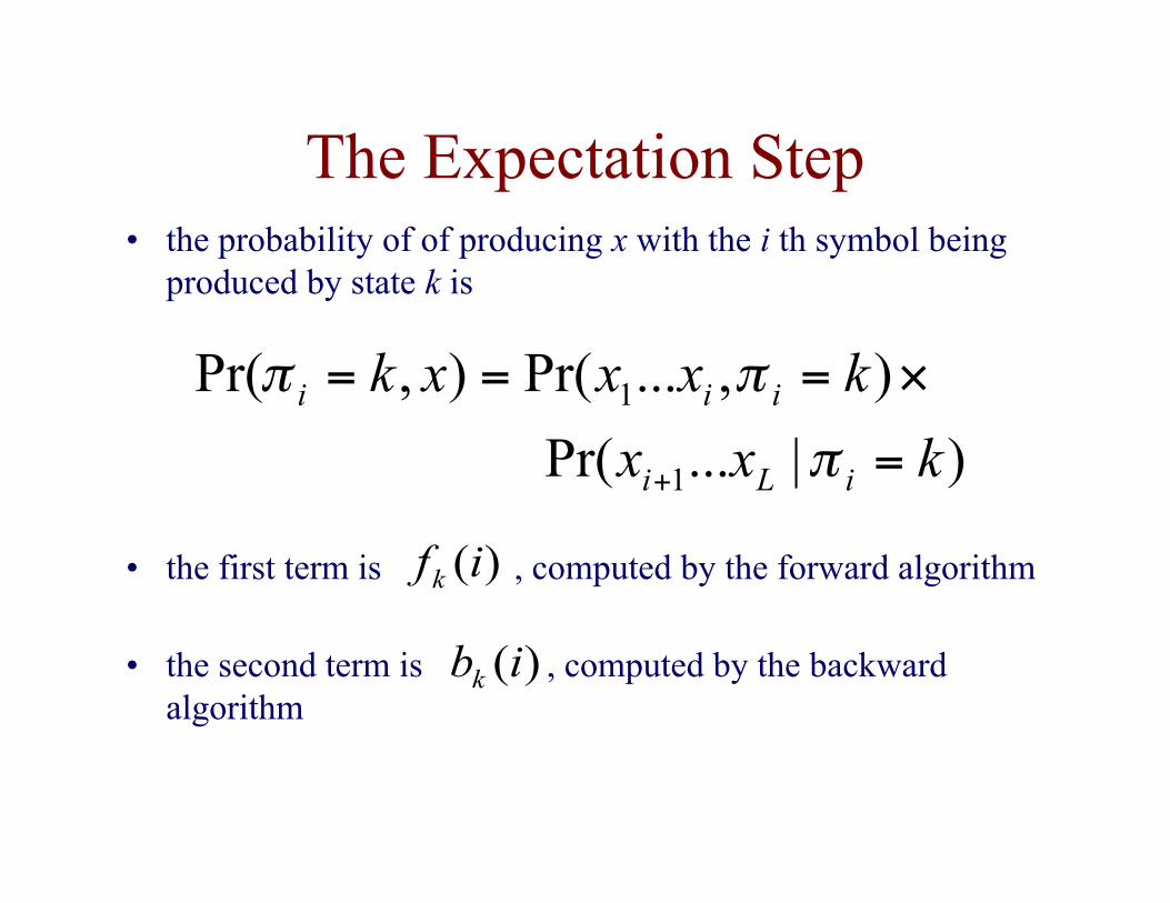
The Expectation Step• the probability of of producing x with the i th symbol being
produced by state k is
)|...Pr(
),...Pr(),Pr(
1
1
kxx
kxxxk
iLi
iii
=
×===
+ π
ππ
• the first term is , computed by the forward algorithm)(ifk
• the second term is , computed by the backwardalgorithm
)(ibk
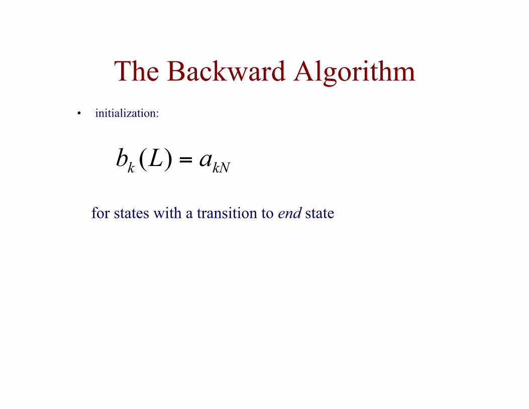
The Backward Algorithm• initialization:
kNk aLb =)(
for states with a transition to end state
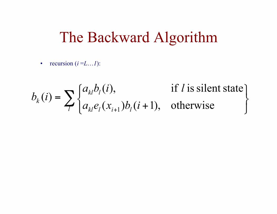
The Backward Algorithm
• recursion (i =L…1):
otherwise ),1()(
statesilent is if ,)()(
1∑
+=
+l lilkl
lklk ibxea
libaib
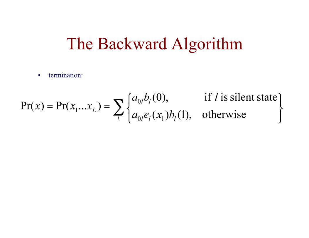
The Backward Algorithm
• termination:
otherwise ),1()(
statesilent is if ,)0()...Pr()Pr(
10
01 ∑
==l lll
llL bxea
lbaxxx
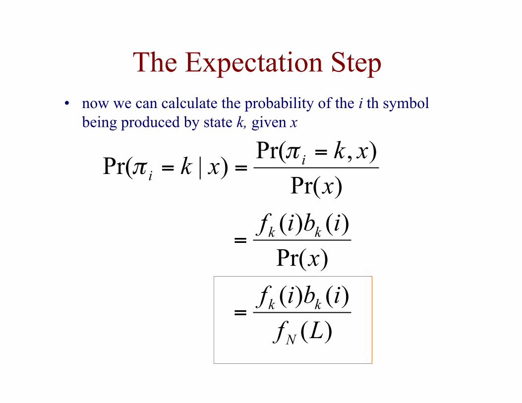
The Expectation Step
)(
)()(
)Pr(
)()(
)Pr(
),Pr()|Pr(
Lf
ibif
x
ibif
x
xkxk
N
kk
kk
ii
=
=
===
ππ
• now we can calculate the probability of the i th symbolbeing produced by state k, given x
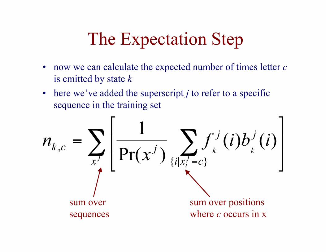
The Expectation Step
∑ ∑
=
=jk
ji
k
x
j
cxi
jjck ibifx
n )()()Pr(
1
}|{,
• now we can calculate the expected number of times letter cis emitted by state k
• here we’ve added the superscript j to refer to a specificsequence in the training set
sum oversequences
sum over positionswhere c occurs in x
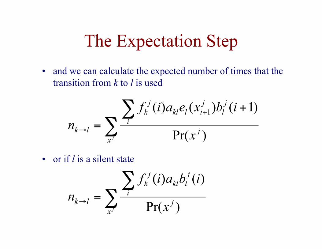
The Expectation Step
∑∑ +
=+
→jx
j
jl
jilkl
i
jk
lk x
ibxeaifn
)Pr(
)1()()( 1
• and we can calculate the expected number of times that thetransition from k to l is used
• or if l is a silent state
∑∑
=→jx
j
jlkl
i
jk
lk x
ibaifn
)Pr(
)()(
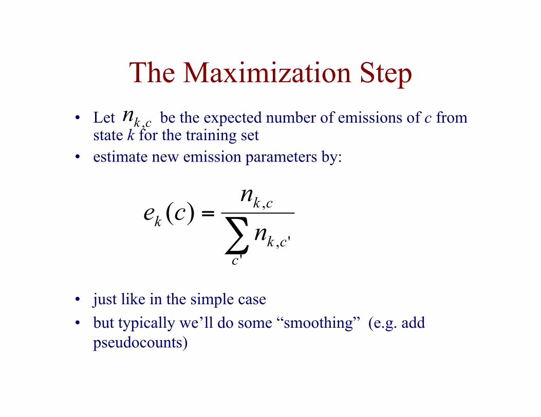
The Maximization Step
∑=
'',
,)(
cck
ckk n
nce
ckn ,• Let be the expected number of emissions of c fromstate k for the training set
• estimate new emission parameters by:
• just like in the simple case
• but typically we’ll do some “smoothing” (e.g. addpseudocounts)
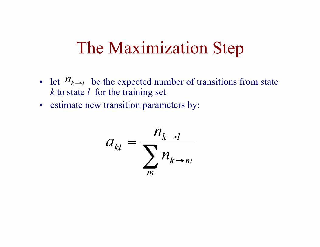
The Maximization Step
∑ →
→=
mmk
lkkl n
na
lkn →• let be the expected number of transitions from statek to state l for the training set
• estimate new transition parameters by:
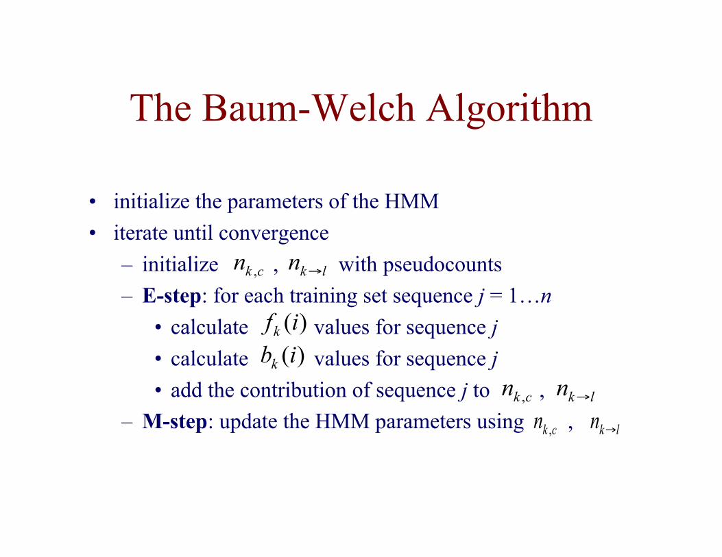
The Baum-Welch Algorithm
• initialize the parameters of the HMM
• iterate until convergence
– initialize , with pseudocounts
– E-step: for each training set sequence j = 1…n
• calculate values for sequence j
• calculate values for sequence j
• add the contribution of sequence j to ,
– M-step: update the HMM parameters using ,
ckn , lkn →
)(ifk)(ibk
ckn , lkn →
ckn , lkn →
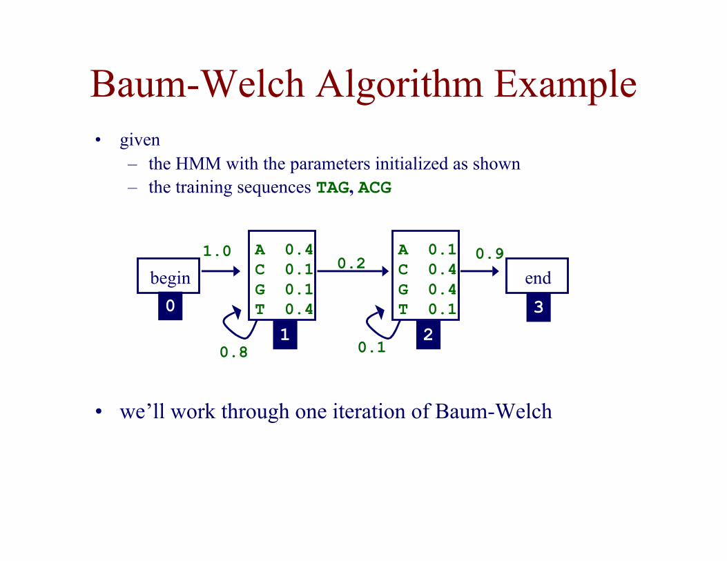
Baum-Welch Algorithm Example• given
– the HMM with the parameters initialized as shown– the training sequences TAG, ACG
A 0.1C 0.4G 0.4T 0.1
A 0.4C 0.1G 0.1T 0.4
begin end
1.0
0.1
0.90.2
0.8
0 321
• we’ll work through one iteration of Baum-Welch
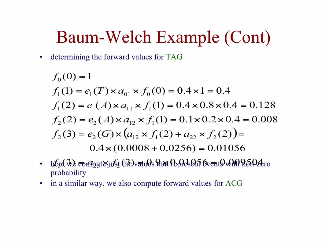
Baum-Welch Example (Cont)• determining the forward values for TAG
• here we compute just the values that represent events with non-zeroprobability
• in a similar way, we also compute forward values for ACG
( )
009504.001056.09.0)3()3(
01056.0)0256.00008.0(4.0
)2()2()()3(
008.04.02.01.0)1()()2(
128.04.08.04.0)1()()2(
4.014.0)0()()1(
1)0(
2233
22211222
11222
11111
00111
0
=×=×=
=+×
=×+××=
=××=××=
=××=××=
=×=××=
=
faf
fafaGef
faAef
faAef
faTef
f
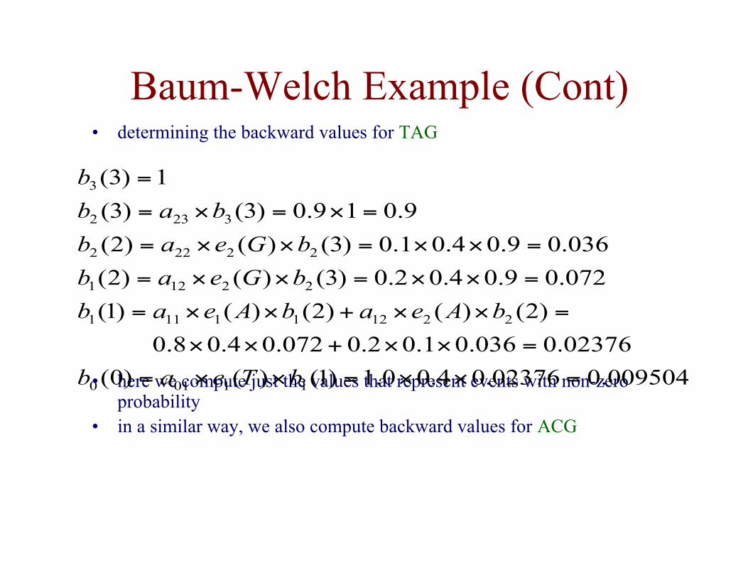
Baum-Welch Example (Cont)• determining the backward values for TAG
• here we compute just the values that represent events with non-zeroprobability
• in a similar way, we also compute backward values for ACG
009504.002376.04.00.1)1()()0(
02376.0036.01.02.0072.04.08.0
)2()()2()()1(
072.09.04.02.0)3()()2(
036.09.04.01.0)3()()2(
9.019.0)3()3(
1)3(
11010
221211111
22121
22222
3232
3
=××=××=
=××+××
=××+××=
=××=××=
=××=××=
=×=×=
=
bTeab
bAeabAeab
bGeab
bGeab
bab
b
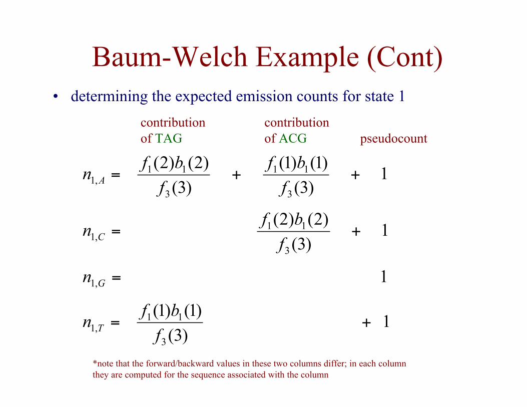
Baum-Welch Example (Cont)• determining the expected emission counts for state 1
1 )3(
)1()1(
)3(
)2()2(
3
11
3
11,1 ++=
f
bf
f
bfn A
1 )3(
)2()2(
3
11,1 +=
f
bfn C
1 )3(
)1()1(
3
11,1 +=
f
bfn T
1 ,1 =Gn
contributionof TAG
contributionof ACG pseudocount
*note that the forward/backward values in these two columns differ; in each column they are computed for the sequence associated with the column
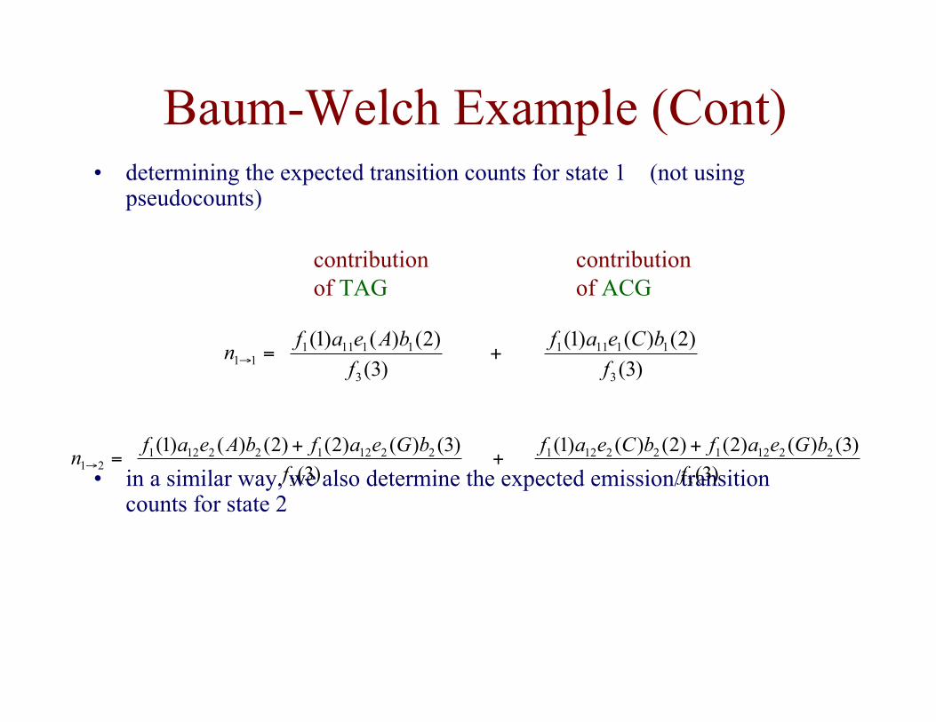
Baum-Welch Example (Cont)• determining the expected transition counts for state 1 (not using
pseudocounts)
• in a similar way, we also determine the expected emission/transitioncounts for state 2
)3(
)2()()1(
)3(
)2()()1(
3
11111
3
1111111 f
bCeaf
f
bAeafn +=→
contributionof TAG
contributionof ACG
)3(
)3()()2()2()()1(
)3(
)3()()2()2()()1(
3
2212122121
3
221212212121 f
bGeafbCeaf
f
bGeafbAeafn
++
+=→
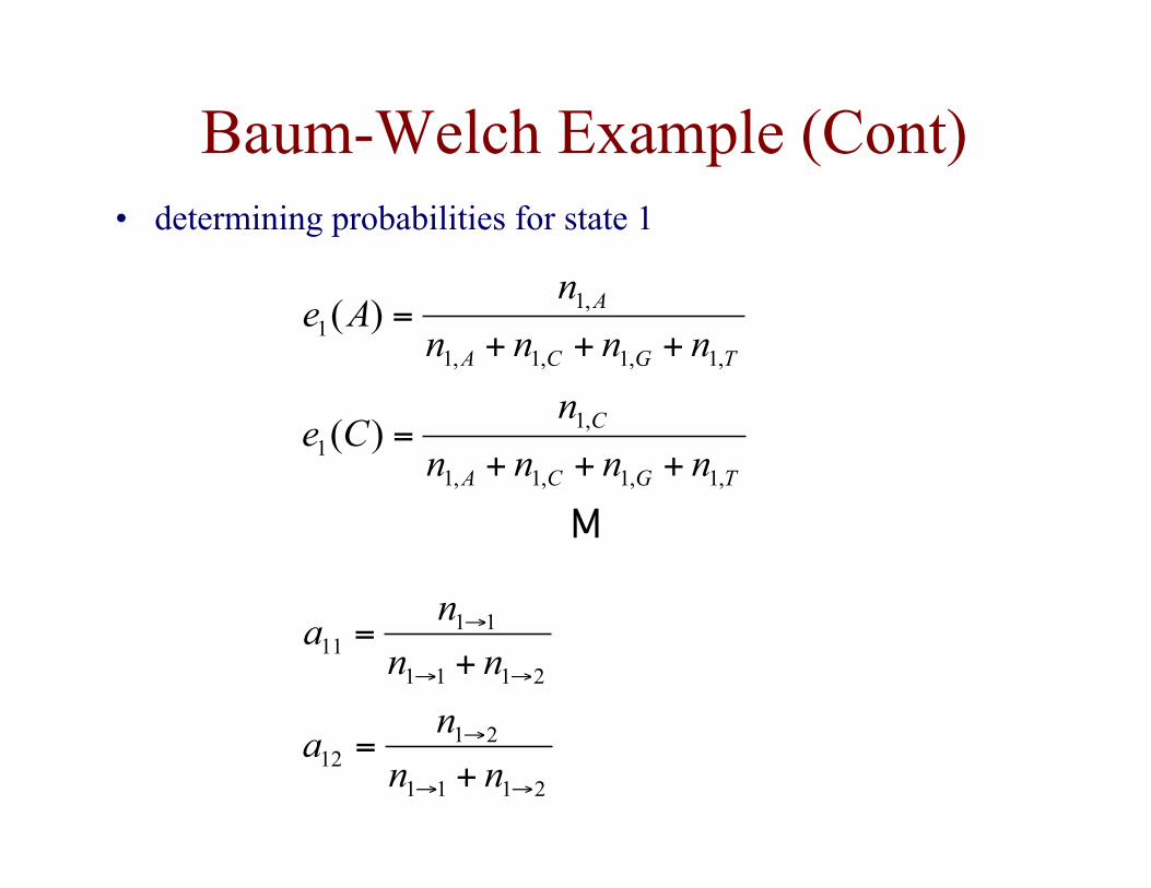
Baum-Welch Example (Cont)• determining probabilities for state 1
M
)(
)(
,1,1,1,1
,11
,1,1,1,1
,11
TGCA
C
TGCA
A
nnnn
nCe
nnnn
nAe
+++=
+++=
2111
2112
2111
1111
→→
→
→→
→
+=
+=
nn
na
nn
na
Markov Models Summary• we considered models that varied in terms of order, in/homogeneity,
hidden state
• three DP-based algorithms for HMMs: Forward, Backward and Viterbi
• we discussed three key tasks: learning, classification and segmentation
• the algorithms used for each task depend on whether there is hiddenstate (correct path known) in the problem or not
Comments on Markov Models• there are many successful applications in computational
biology– gene recognition and associated subtasks– protein family modeling– motif modeling– etc.
• there are many variants of the models/algorithms weconsidered here (some of these are covered inBMI/CS 776)– fixed length motif models– semi-markov models– stochastic context free grammars– Gibbs sampling for learning parameters