Embed Size (px)
Citation preview

Marketmaking Middlemen∗
Pieter Gautier † Bo Hu‡ Makoto Watanabe§
† ‡ § VU University Amsterdam, Tinbergen Institute
May 10, 2015
Very Preliminary
Abstract
This paper develops a model in which market structure is determined endogenously
by the choice of intermediation mode. We consider two representative business modes
of intermediation that are widely used in real-life markets: one is a market-making
mode by which an intermediary offers a platform for buyers and sellers to trade by
their own; the other is a middleman mode by which an intermediary holds inventories
which he stocks from sellers for the purpose of reselling to buyers. In our model,
buyers and sellers have an option of searching in an outside market as well as using the
service offered by a monopolistic intermediary. We derive the conditions under which
the mixture of the two intermediation modes is selected over an exclusive use of either
of the modes.
Keywords: Middlemen, Marketmakers, Platform, Search
JEL Classification Number:D4, F1, G2, L1, L8, R1
∗We thank seminar and conference participants at U Essex, U Bern, U Zurich, and the Symposium on JeanTirole 2014 for useful comments.†VU University Amsterdam, Tinbergen Institute, Address: Department of Economics, VU Amsterdam, De
Boelelaan 1105, NL-1081 HV Amsterdam, The Netherlands, [email protected]‡VU University Amsterdam, Tinbergen Institute, Address: Department of Economics, VU Amsterdam, De
Boelelaan 1105, NL-1081 HV Amsterdam, The Netherlands, [email protected]§VU University Amsterdam, Tinbergen Institute, Address: Department of Economics, VU Amsterdam, De
Boelelaan 1105, NL-1081 HV Amsterdam, The Netherlands, [email protected]
1
1 Introduction
This paper considers a framework in which market structure is determined by the intermediation
service offered to customers. We consider two representative business modes of intermediation
that are widely used in real-life markets. In one mode, an intermediary acts as a middleman (or
a merchant), who is specialized in buying and selling by his own account and typically operates
by holding inventory (e.g. supermarkets, and traditional brick and mortar retailers). In the other
mode, an intermediary acts as a marketmaker, who offers a marketplace or a platform where the
participating buyers and sellers trade with each other (e.g. eBay).
In most real-life markets, however, intermediaries are not one of those extremes but operate
both as a middleman and a marketmaker at the same time. This is what we call a marketmaking
middleman.1 For example, the well-known electronic intermediary Amazon, one of the largest
marketmaking middlemen nowadays, started off as a pure middleman, buying and reselling prod-
ucts in its own name since its founding in 1994. In the early 2000s, Amazon moved toward a
marketmaker, by allowing other suppliers to participate as independent sellers. In 2014, those
independent sellers accounted for 50% of gross merchandise volume of Amazon. Similar operation
patterns are used by both Rakuten and JD.com, which are Amazon’s counterparts in Japan and
China. Other examples of marketmaking middlemen include real-estate agents, dealer/brokers in
financial markets, and department stores.2
We present a model in which the intermediated-market structure is determined endogenously
as a result of the strategic choice of a monopolistic intermediary. In our model, there are two
markets open to agents, one is an intermediated market operated by the intermediary, and the
other is a decentralized market where buyers and sellers search randomly. The intermediated
market combines two business modes: acting as a middleman, the intermediary is prepared to
serve many buyers at a time by holding inventories; acting as a marketmaker, the intermediary
offers a platform. The intermediary can choose how to allocate the attending buyers among these
two business modes.
1In the finance literature, different terminologies are used to classify the type of intermediaries: brokers refer tointermediaries who do not trade for their own account, but act merely as conduits for customer orders, akin to ourmarketmakers; dealers refer to intermediaries who do trade for their own account, akin to our middlemen/merchants.The marketmakers (or specialists) in financial markets correspond broadly to our market-making middlemen, sincethey quote prices to buy or sell the asset as well as take market positions.
2In particular, real-estate agents match buyers and sellers, and also stock properties themselves for sale;dealer/brokers in financial markets engage in trading securities on behalf of clients as well as for their own ac-counts; some department stores also rent shelf spaces to manufacturers. Further examples can be found in Hagiuand Wright (2015).
2
In either way of intermediated trade, we formulate the intermediated market as a directed
search market in order to feature the intermediary’s technology of spreading price and capacity
information efficiently.3 In addition, this approach enables us to highlight the middleman’s ad-
vantage in the high selling capacity that mitigates search frictions and provides customers with
proximity. Thus, the middleman mode outperforms the marketmaker mode in allocation effi-
ciency. The decentralized market represents an individuals’ outside option that determines the
lower bound of their market utility.
With this set up, we consider two situations, single-market search versus multiple-market
search. With the single market search, agents have to choose which market to search in advance,
either the decentralized market or the intermediated market. This implies that the intermediary
needs to subsidize either buyers or sellers with their expected value in the decentralized market,
but once they participate, the intermediated market operates without fear of competitive pressure
outside. In this situation, the intermediary can extract the individual surplus monopolistically for
each realized transaction. This can be done either by setting a monopolistic intermediation fee as
a marketmaker, or by charging a monopolistic price for the inventory as a middleman – in either
way, the per-transaction profits are the same. Given the middleman mode is more efficient in
realizing transactions, the intermediary uses the middleman-mode exclusively when agents search
a single market.
When agents are allowed to search multiple markets, attracting buyers and sellers becomes less
costly compared to the single-market search case — the intermediary does not need to subsidy
either of the sides to induce participation. However, this time, the prices/fees charged in the
intermediated market must be acceptable relative to the available option in the decentralized
market. Thus, with the multiple-market search, the outside option creates competitive pressure
to the overall intermediated market. On the one hand, a higher capacity of the middleman leads
to a larger number of successful transactions in the intermediated market. This happens due to
the demand stimulating effect: a higher capacity induces more buyers to buy from the middleman,
and fewer buyers to search in the platform, which increases the intermediary’s profit. On the other
hand, the demand effect makes sellers less likely to be successful in the platform, so that more
sellers are available when a buyer attempts to search in the decentralized market. Accordingly, the
buyers expect a higher value from the decentralized market, which causes a competitive pressure on
3Using the search function in the Amazon website, for example, one can receive instantly all relevant informationsuch as prices, stocks of individual sellers and Amazon’s inventories.
3

the price that the intermediary can charge. Hence, the intermediary trade-offs a larger quantity
against lower price/fees to operate as a larger-scaled middleman. This trade-off pins down an
optimal structure of intermediation modes.
In real-life economy, the single-market search may correspond to the traditional search tech-
nology for supermarkets or brick and mortar retailers. Over the course of shopping trip under
such a circumstance, consumers usually have to search, buy and even transport the purchased
products during a fixed amount of time. Given the time constraint, they visit a limited number
of shops – typically one supermarket –, and appreciate the proximity provided by its inventory.
In contrast, the multi-market search may be related to the advanced search technologies available
in the digital economy. Such a technology allows the online-customers to search with ease and
convenience, and to compare various options. A similar can happen in the market for durable
goods such as housing or expensive items where customers are usually exposed to the market for
a sufficiently long time period to ponder multiple available options.
The comparison of the above two cases delivers an interesting policy implication of intermedi-
ated markets. In our economy, the optimal business mode from the social planner’s viewpoint is
the middleman mode because it minimizes market frictions and can implement an efficient trade.
In the presence of outside competition, however, using a platform can be profitable for the inter-
mediary and it reduces its inventory from the efficient level. Hence, competition for intermediation
can deteriorate efficiency and welfare.
This paper contributes to two strands of literature. One is the literature of middlemen de-
veloped by Rubinstein and Wolinsky (1987), Duffie, Garleanu, and Pedersen (2006), Lagos and
Rocheteau (2009), Shevichenko (2004), Johri and Leach (2002), Masters (2007), and Wong and
Wright (2014).4 Using a directed search approach, Watanabe (2010, 2013) provide a model of an
intermediated market operated by middlemen with high inventory holdings. The middlemen’s high
capacity enables them to serve many buyers at a time, thus to lower the likelihood of stock-out,
which generates a retail premium of inventories. This mechanism is adopted by the middleman in
our model as well. Hence, if intermediation fees are not available, then our model is a simplified
version of Watanabe where we added an outside market. It is worth mentioning that in Watanabe
4Rubinstein and Wolinsky (1987) show that an intermediated market can be active under frictions, when itis operated by middlemen who have an advantage in the meeting rate over the original suppliers. Given someexogenous meeting process, two main reasons have been considered for the middlemens advantage in the rate ofsuccessful trades: a middleman may be able to guarantee the quality of goods (Biglaiser, 1993, Li, 1998), or tosatisfy buyers demand for a varieties of goods (Shevichenko, 2004). While these are clearly sound reasons forthe success of middlemen, the buyers search is modeled as an undirected random matching process, thereby themiddlemens capacity cannot influence buyers search decisions in these models.
4

(2010, 2013), the middleman’s inventory is modeled as a discrete unit, i.e., a positive integer, so
that the middlemen face a non-degenerate distribution of their selling units as other sellers do.
In contrast, we model the inventory as measured by mass, assuming more flexible inventory tech-
nologies, so that the middleman faces a degenerate distribution of sales. This simplification allows
us to characterize the middleman’s profit maximizing level of inventory – in Watanabe (2010)
the inventory level of middlemen is determined by aggregate demand-supply balancing. Recently,
Holzner and Watanabe (2015) study a labor market equilibrium using a directed search approach
to model a job-brokering service (i.e., a market-making service), offered by Public Employment
Agencies, but the choice of intermediation mode is not the scope of their paper.
The other related strand is the two-sided market literature, e.g. Rochet and Tirole (2003,
2006), Caillaud and Jullien (2003), Rysman (2004), Armstrong (2006), Hagiu (2006) and Weyl
(2010).5 The critical feature of platform is the presence of the cross-group externality, i.e. the
participants’ expected gains from a platform depend positively on the number of participants on
the other side of it. When such a cross-group externality exists, the marketmaker can use “divide-
and-conquer” strategies, namely, subsidizing one group of participants in order to attract another
group and extract the ensuing externality benefit (see, Caillaud and Jullien, 2003). This strategy
is adopted by the intermediary in our model as well. Broadly speaking, if there is no middleman
mode, then our model is a directed search version of Caillaud and Jullien (2003) in combination
with a decentralized market.
Finally, without considering search frictions, Hagiu and Wright (2015) study the profitability
of intermediation modes as is determined by marketing activities. In their model, it is assumed
that the owner of a product has private information on how effective their marketing activity
will be. They show that the optimal design of intermediation mode is determined, among others,
by the cross-product spillovers of marketing activity, and the degree of owners’ informational
advantage. For each product, an intermediary only takes the preferred extreme mode instead of a
hybrid one, and their theory explains which products the intermediary should offer in which mode.
In contrast, with considering search frictions, we show that even for a homogeneous product, a
hybrid intermediation mode can occur in equilibrium. Our theory explains how the intermediated
market is structured depending on the search/competitive environment. Rust and Hall (2003)
5Closely related papers based on a similar spirit can be found in Baye and Morgan (2001), Rust and Hall(2003), Parker and Van Alstyne (2005), Nocke et al. (2007), Galeotti and Moraga-Gonzalez (2009), Loertscher andNiedermayer (2012) and Edelman and Wright (2015). For earlier contributions of this strand of literature, see, e.g.,Stahl (1988), Gehrig (1993), Yavas (1994, 1996), Spulber (1996) and Fingleton (1997).
5
consider two types of intermediaries, one is “middlemen” whose market requires costly search and
a monopolistic “market maker” who offers a frictionless market. They show that agents segment
into different markets depending on heterogeneous production costs and consumption values, thus
these two types of intermediaries can coexist in equilibrium. Their model is very different from
ours in many respects. For instance, selling capability and inventory does not play any role in their
formulation of sequential search, but it is the key ingredient in our model. Further, we show that
a monopolistic intermediary can pursue different types of intermediation modes even faced with
homogeneous agents. We believe a similar property would survive in an extended environment
with entry or oligopolistic intermediaries.
The rest of the paper is organized as follows. Section 2 presents the basic setup. Section 3
studies the choice of intermediation mode for single-market technology and it provides a benchmark
of our economy. Section 4 extends the analysis to allow for multiple-market technology and gives
the key finding of the paper. Section 5 discusses the welfare and other modeling issues. Section 6
concludes. Some proofs are in the Appendix.
2 Setup
We consider a large economy with two types of agents: a mass B of buyers and a mass S of
sellers. Agents of each type are homogeneous. Each buyer has unit demand of a homogeneous
good, and each seller has a production technology of that good. The consumption value for the
buyer is normalized to 1. The marginal production cost is constant and without loss of generality,
we normalize it to zero. Sellers are able to produce as much as they want but their selling/trading
capability is limited so that each seller can sell only one unit of the good.
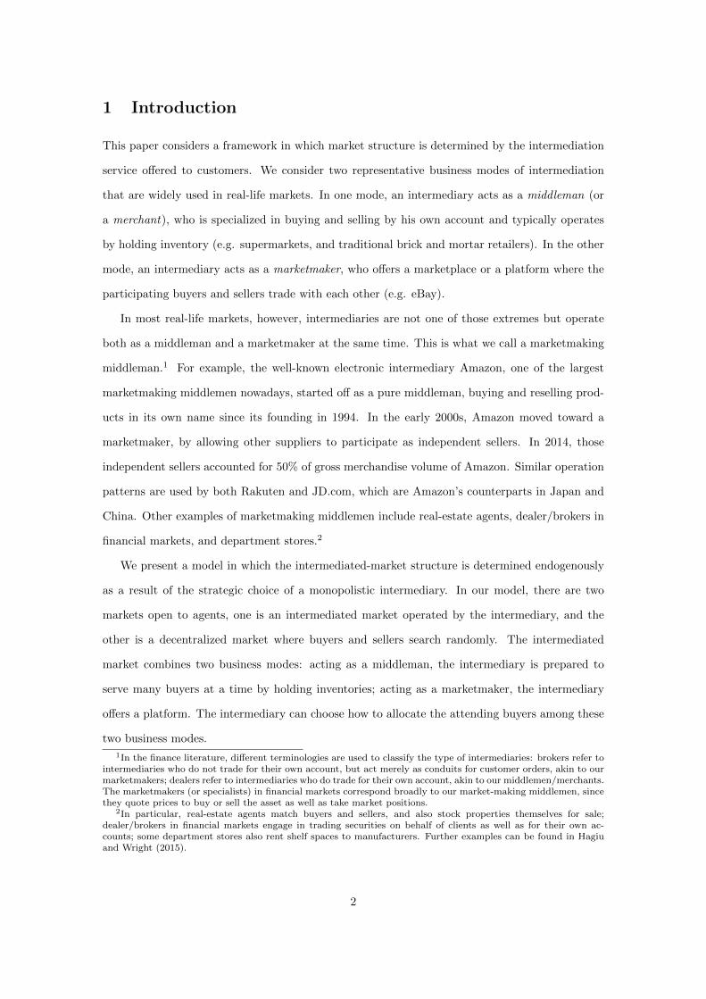
There are two retail markets, a centralized market and a decentralized market (see Figure
1). The decentralized market (hereafter D market) is featured by random matching and bilateral
bargaining. We assume that the flow of contacts between sellers and buyers in the D market is
given by a matching technology M = M(BD, SD) where BD and SD denote the amount of buyers
and sellers that actually participate in the D market. The function M is continuous, nonnegative,
with M(0, SD) = M(BD, 0) = 0 for all BD, SD ≥ 0. Without loss of generality, we further assume
that for BD, SD > 0 a buyer finds a seller with probability λb = M(BD,SD)BD
and a seller finds a
buyer with probability λs = M(BD,SD)SD
, satisfying BDλb = SDλs and λb, λs ∈ (0, 1) is a constant.
This linear matching technology is extended to general non-linear matching functions in Section
6

6. Matched partners follow an efficient bargaining process, which yields a linear sharing of the
total surplus, with β ∈ (0, 1) as the share for the buyer, and 1− β for the seller.
The centralized market (hereafter C market) is operated by a monopolistic intermediary. The
intermediary can perform two different intermediation activities. As a middleman, he purchases
a good from sellers in a wholesale market, and holds it as an inventory to resell to buyers. The
wholesale market is operated by sellers, who have no limit in producing the good. We assume
the wholesale market to be competitive so that the inventory demand of the middelman is always
satisfied at the competitive wholesale-price equal to marginal production cost (normalized to
zero). We will describe later the case with positive production costs. The middleman can stock
inventories in advance so that he is prepared to serve buyers the retail markets.
As a marketmaker, he does not buy and sell but instead provides a platform where buyers and
sellers can interact with each other for trade upon paying fees.
We assume that the C market is subject to directed search frictions. In a directed search
environment, the prices and capacities of all the individual suppliers are publicly observable.
The intermediary has technologies to spread this information. Still, given that individual buyers
cannot coordinate their search activities, the limited selling capacity of individual sellers creates
a possibility that some units remain unsold and some demands are not satisfied. This is the
standard notion of directed search frictions, see e.g., Peters (1991, 2001), Moen (1997), Acemoglu
and Shimer (1999), Burdett, Shi and Wright (2001), Albrecht, Gautier, and Vroman (2006), and
Guerrieri, Shimer and Wright (2010), and in this sense, the platform in our economy is frictional.
As will be detailed below, however, there is no such a friction in the middleman’s trade since
its inventory management technologies allow for the selling capability to be comparable to the
population of potential buyers in magnitude.
The timing of events is as follows.
1. Two retail markets, a C market and a D market, open. In the C market, the intermediary
announces a set of fees F ≡{f b, fs, gb, gs
}for the platform, where f b, fs ∈ [0, 1] is a trans-
action fee charged to a buyer or a seller, respectively, and gb, gs ∈ [−1, 1] is a registration
fee charged to a buyer or a seller, respectively.
2. Observing the announced fees F , buyers and sellers simultaneously decide whether to par-
ticipate in the C market. We consider two different search technologies of agents: the
single-market search, with which agents can attend only one market, and the multi-market
7
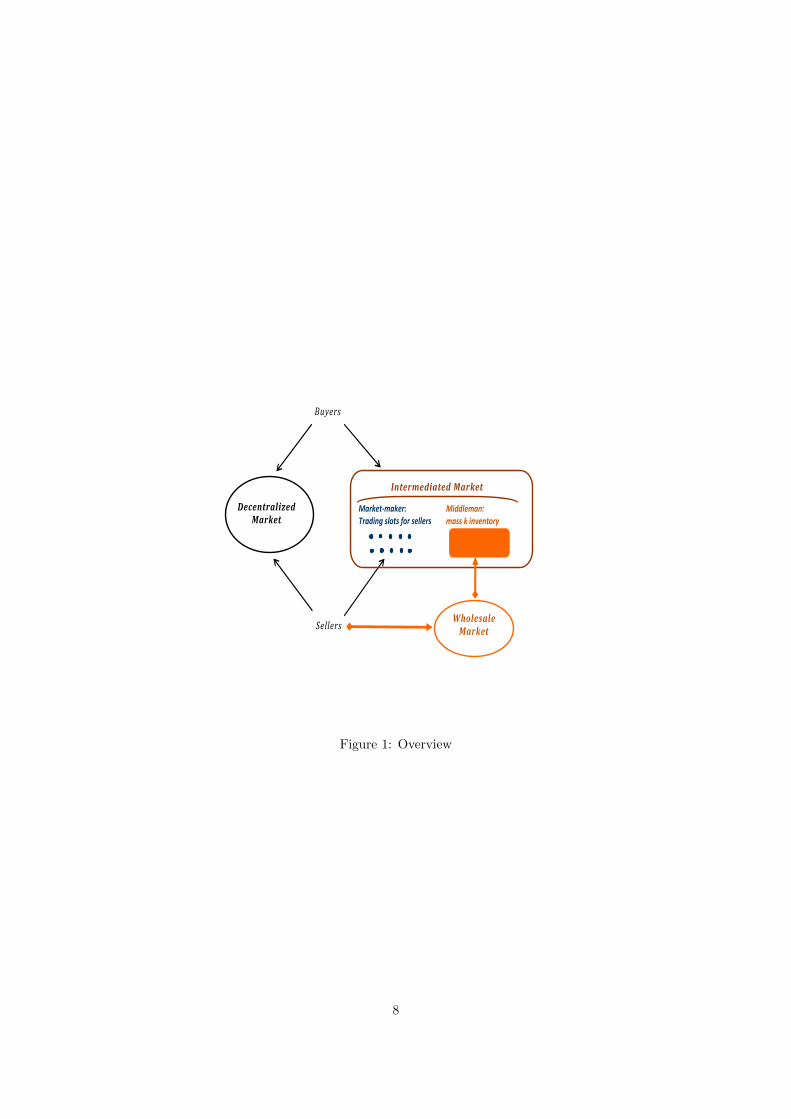
Pure marketmakerPure middleman Marketmaking middleman
DecentralizedMarket
Sellers
Buyers
WholesaleMarket
SupermarketsRetailersiTunes
eBay, TaobaoApple storeGoogle Play
Amazon, bol.com, RakutenReal estate agentsDealers in financial markets
Market-maker:Trading slots for sellers
Middleman:mass k inventory
Intermediated Market
Figure 1: Overview
8

search with which agents can attend both markets.
3. In the C market, the participating buyers, sellers and middleman are engaged in a directed
search game. In the D market, agents search randomly and follow the efficient bargaining
sharing rule for the trade surplus.
We work backward and first characterize a directed search equilibrium in the C market. Sup-
pose that a mass B buyers and a mass S sellers have decided to participate in the C market,
and that the intermediary has stocked K ∈ [0, B] ⊂ R+ inventories. Then, the C market has the
following stages. In the first stage, all the suppliers, i.e., the participating sellers with the unit
selling-capacity and the middleman with the K capacity, simultaneously post a price which they
are willing to sell at. Observing the prices and the capacities, all buyers simultaneously decide
which supplier to visit in the second stage. Each buyer can visit one supplier. Assuming buyers
cannot coordinate their actions over which supplier to visit, we follow Peters (1991, 2001) and
investigate a symmetric equilibrium where all buyers use an identical visiting strategy for any
configuration of the announced prices. Each individual seller has a queue xs of buyers with an
equilibrium price ps and the middleman has a queue xm of buyers with an equilibrium price pm.
These quantities should satisfy two requirements. The first requirement is the accounting identity,
Sxs + xm = B, (1)
which states that the number of buyers visiting individual sellers Sxs and the middleman xm
should sum up to the total population of participating buyers B. The second requirement is the
buyers’ optimal search:
xm =
B if V m(B) ≥ V s(0)
(0, B) if V m(xm) = V s(xs)
0 if V m(0) ≤ V s(BS ),
(2)
where V i(xi) is the equilibrium value of buyers to visit a seller if i = s and the middleman if
i = m (yet to be specified below). Conditions (1) and (2) define the counterpart for xs ∈ [0, BS ].
As for the intermediation mode in the C market, we shall adopt the following terminology.
Definition 1 Suppose B buyers and S sellers participate in the C market. Then, we say that the
intermediary acts as:
9

• a pure middleman if xm = B (⇔ xs = 0);
• a market-making middleman if xm ∈ (0, B) (⇔ xs ∈ (0, BS )).
• a pure market-maker if xm = 0 (⇔ xs = BS );
3 Single-market search
We start analysis for the single-market search technologies where agents can participate in only
one market.
Given the participation of B buyers and S sellers, if agents have single-market search tech-
nologies, then the intermediary will act as a pure middleman by selecting f∗ = f b∗ + fs∗ > 1 and
K∗ = B. This leads to the highest possible profits with pm = 1 in the C market,
Π(pm, f∗,K∗) = B.
Under these price and fees, all the buyers buy from the middleman, xm = B, and the platform
is inactive, xs = 0. This is indeed an equilibrium since V m(B) = 0 > V s(0) under pm = 1 and
f∗ > 1, and for any ps ∈ [0, 1], sellers make zero profit in the C market.
In what follows, we illustrate that creating an active platform is not profitable. Suppose that
intermediation fees are f = f b + fs ≤ 1. Then, the platform generates a non-negative trade
surplus 1− f ≥ 0. An active platform will be frictional and is described as follows.
Given the symmetric strategy of buyers’ search, the number of buyers visiting one individual
seller is a random variable, denoted by N , which has a Poisson distribution, Prob[N = n] = e−xxn
n! ,
if he has an expected queue of buyers x ≥ 0. Hence, the limiting selling capacity (i.e., an ability
to sell only a single unit) implies that a seller with an expected queue xs ≥ 0 of buyers has a
probability 1 − e−xs of successfully selling the good, where e−xs
= Prob[N = 0]. The expected
value of a seller with a price ps and an expected queue xs in the platform, denoted by W = W (xs),
is
W (xs) = (1− e−xs
)(ps − fs), (3)
where the seller succeeds with probability 1−exs in which case he receives ps minus the transaction
fee fs. If not successful, then he receives zero payoff. The expected value of a buyer who visits a
10

seller with a price ps and an expected queue xs in the platform is
V s(xs) =1− e−xs
xs(1− ps − f b), (4)
where the buyer is served with probability 1−e−xs
xs and obtains 1 − ps minus the transaction fee
f b. If not served, then his payoff is zero.
The middleman sector is described as follows. If a middleman’s price pm ∈ [0, 1] attracts
xm ≥ 0 buyers, then since the middleman has a mass of inventory, the expected profit from the
middleman sector is given by min{K,xm}pm. The expected value of buyers to visit the middleman
is
V m(xm) = min{ Kxm
, 1}(1− pm). (5)
There are two cases for active platform. First, suppose that the intermediary shuts down
the middleman sector, by holding no inventory at all K = 0, so that all the buyers search in
the platform, i.e., xm = 0 and xs = BS . Then, the intermediary makes an expected revenue
S(1− e−xs)f in the platform but nothing from the middleman sector. The profits are
Π(pm, f, 0) = S(1− e−BS )f < B = Π(1, f∗,K∗)
for all f ≤ 1, since 1− e−BS < BS . Hence, the exclusive use of the platform is not profitable. Next,
suppose that the intermediary make both sectors active with some pm ∈ [0, 1] and K ∈ (0, B], i.e.,
xm ∈ (0, B) and xs ∈ (0, BS ) that satisfy the add-up requirement (1) and the indifferent condition
(2). Then, the resulting profit satisfies
Π(pm, f,K) = S(1− e−xs
)f + min{K,xm}pm
< Sxsf + xmpm
≤ (Sxs + xm) max{f, pm}
≤ B = Π(1, f∗,K∗),
for all f ≤ 1 and pm ≤ 1, where the last inequality from the add-up condition (1), Sxs +xm = B.
Hence, this is not profitable either. All in all, any active platform is not profitable.
The intuition behind the occurrence of a pure middleman is as follows. Given the frictions in
the intermediated platform, a larger middleman sector creates more transactions. To guarantee
that all participating buyers are in the middleman sector, the intermediary can shut down the
platform by setting high enough fees f > 1, and exploit them by charging pm = 1 to the inventory.
11

In a nutshell, the middleman’s inventory is the efficient way to allocate the good and, if agents
search within a single market, then the intermediary is guaranteed with the full surplus of it.
We now consider how the intermediary can induce agents to participate in the C market. As
each retail-market is faced with two-sided participation, an issue arises for the belief-dependent
multiplicity of equilibria – the participation decision of buyers (sellers) depends on their belief
on the participation of sellers (buyers). For the selection of beliefs, we follow the literature of
two sided-market and assume that agents hold pessimistic beliefs on the participation decision of
agents on the other side of the market (Caillaud and Jullien, 2003). Accordingly, agents believe
that the intermediary would never hold inventory unless the C market attracts some buyers. For
instance, a pessimistic belief of sellers means that sellers believe the number of buyers participating
in the C market is zero whenever
λbβ > −gb,
where λbβ is the expected payoff of buyers in the D market and it is believed that the C market is
empty so that all buyers receive in the C market is −gb (it is a participation subsidy when gb < 0).
To induce participation under those beliefs, the best the intermediary can do is to use a divide-
and-conquer strategy, denoted by h. To divide buyers and conquer sellers, referred to as h = DbCs,
it is required that
Db : −gb ≥ λbβ, (6)
Cs : W − gs ≥ 0. (7)
The divide-condition Db tells us that the intermediary should subsidy the participating buyers so
that they are guaranteed at least what they would get in the D market, even if the C market is
empty. This makes sure that buyers will join the C market. The conquer-condition Cs guarantees
the participation of sellers, by giving them a nonnegative payoff – the participation fee gs ≥ 0
should be no greater than the expected value of sellers in the C market, W ≥ 0. Observing
that the intermediary offers buyers with a sufficiently generous subsidy, sellers understand that
all buyers are in the C market, the D market is empty, and so the expected payoff from the D
market is zero. Here, the expected value of sellers in the C market W is defined under the sellers’
rational expectation that the intermediary will select the inventory level optimally given the full
participation of buyers.
Similarly, a strategy to divide sellers and conquer buyers, referred to as h = DsCb, requires
12
that
Ds : −gs ≥ λs(1− β), (8)
Cb : V − gb ≥ 0. (9)
where V = max{V m(xm), V s(xs)} ≥ 0 is the expected value of buyers in the C market.
Given the participation decision of agents described above, the intermediary’s problem of
determining the intermediation fees F = {f b, fs, gb, gs} for h = {DbCs, DsCb} is described as
Π = maxF,h{Bgb + Sgs + Π(pm, f,K)},
subject to (6) and (7) if h = DbCs, or (8) and (9) if h = DsCb. Here, Bgb and Sgs are participation
fees from buyers and sellers, respectively, and Π(·) is the expected profit in the C market described
above. Under either of the divide-and-conquer strategies, the choice of participation fees gi,
i = b, s, does not influence anyone’s behaviors in the C market. The choice of transaction fees
affects the expected value of agents and hence the participation fees and intermediary’s profits.
However, it does not alter the intuition provided above and a pure middleman remains optimal.
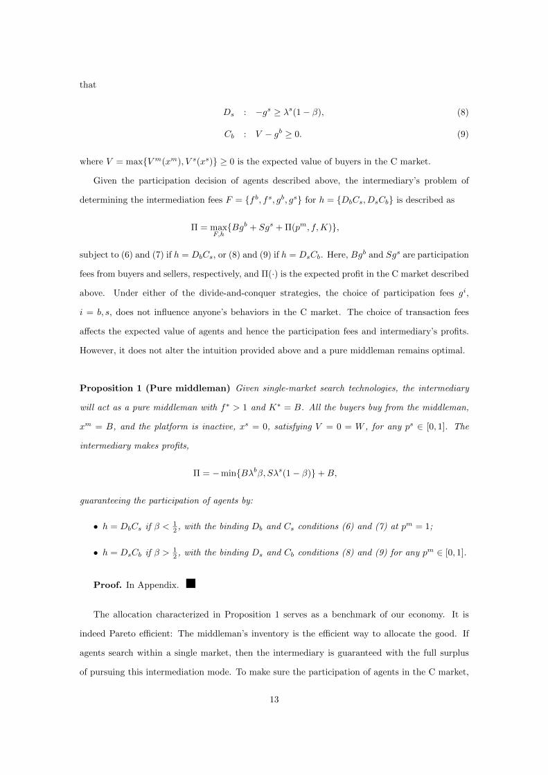
Proposition 1 (Pure middleman) Given single-market search technologies, the intermediary
will act as a pure middleman with f∗ > 1 and K∗ = B. All the buyers buy from the middleman,
xm = B, and the platform is inactive, xs = 0, satisfying V = 0 = W , for any ps ∈ [0, 1]. The
intermediary makes profits,
Π = −min{Bλbβ, Sλs(1− β)}+B,
guaranteeing the participation of agents by:
• h = DbCs if β < 12 , with the binding Db and Cs conditions (6) and (7) at pm = 1;
• h = DsCb if β > 12 , with the binding Ds and Cb conditions (8) and (9) for any pm ∈ [0, 1].
Proof. In Appendix.
The allocation characterized in Proposition 1 serves as a benchmark of our economy. It is
indeed Pareto efficient: The middleman’s inventory is the efficient way to allocate the good. If
agents search within a single market, then the intermediary is guaranteed with the full surplus
of pursuing this intermediation mode. To make sure the participation of agents in the C market,
13
the intermediary can use a divide and conquer strategy to overcome pessimistic beliefs of agents
by subsidizing either side of the market. Which side should be subsidized depends on the outside
option in the D market. If β < 12 then buyers are less costly to convince, and the buyers’ trade
surplus can be exploited fully in the middleman sector by charging pm = 1. If β > 12 then sellers
are less costly to subsidize, and when to exploit the participating buyers does not matter – the
intermediary makes the maximum revenue B for any pm ∈ [0, 1].
4 Multi-market search
In this section, we extend our analysis to multiple-market search technologies where agents can
search both the C market and the D market.
Since agents can search both of the markets, a timing issue arises on which market should
open first. Below, we present the analysis of the setup that the C market opens prior to the D
market. Apart from the fact that this appears to be the most natural setup in our economy, we
are motivated by the first mover advantage of the intermediary: its expected profit is higher if the
C market opens before, rather than after, the D market. Hence, our setup will arise endogenously
if the intermediary is allowed to select the timing of the market sequence to enjoy the first mover
advantage. 6
Directed search equilibrium in the C market: We work backward and first describe a
directed search equilibrium in the C market assuming that there are B buyers and S sellers. As
before any directed search equilibrium in the C market has to satisfy the add-up restriction (1)
and the symmetric search strategy of buyers (2). Given the multiple-market search of agents,
agents expect a non-negative value for the D market when deciding whether or not to accept an
offer in the C market. Hence, whenever the platform is active xs > 0, the set of transaction fees
f i, i = b, s, must satisfy the constraints:
1− ps − f b ≥ λbe−xs
β (10)
ps − fs ≥ λsξ(xm,K)(1− β). (11)
6As a real-life correspondence of such a situation, online retailers have in principle unlimited opening hours aday, whereas such a flexible business practice is physically infeasible offline. In addition, many online retailers areenthusiastic in making their websites fast and easy, providing a wide range of information on merchandize andoffering personalized service such as special offer emails tailored to a customer’s interest, etc. These efforts wouldenhance customer experiences and create loyalty, which may increase their chance to become a first-mover. In arecent study without intermediation, Armstrong and Zhou (2014) show that a seller often makes it harder or moreexpensive to buy its product later than at the first opportunity.
14
The constraint of buyers (10) states that the offered price/fee in the C market is acceptable only
if the offered payoff 1 − ps − f b is no less than the expected value in the D market: the outside
payoff is not zero this time, but is β if he is matched in the D market with a seller who has failed
to trade in the C market. This happens with probability λbe−xs
. Hence, the larger the platform
size xs, the higher the chance that a seller is successful in the C market, and the lower the chance
that a buyer can trade successfully in the D market and the lower his expected outside value.
Similarly, the constraint of sellers (11) states that the payoff in the C market ps − fs should be
no less than the expected value in the D market where ξ(xm,K) represents the probability that
a buyer has failed to trade in the C market and is given by
ξ(xm,K) ≡ 1−(xm
Bηm(xm) +
Sxs
Bηs(xs)
)= 1− 1
B
(min{K,xm}+ S(1− e−(B−xm
S ))),
where ηm(xm) ≡ min{ Kxm , 1} is the probability of the buyer to be served in the middleman sector
and ηs(xs) ≡ 1−e−xs
xs in the platform. In this expression, the terms in the parethesis represent the
expected chance of a buyer to trade in the C market. A buyer has been in the middleman sector
with probability xm
B and served with probability ηm(xm), or in the platform with probability Sxs
B
and served with probability ηs(xs).
We now determine the equilibrium price ps in an active platform, xs > 0. Suppose a seller
deviates to a price p 6= ps that attracts an expected queue x of buyers. Note that given the limited
selling-capacity, this deviation has measure zero and does not affect the expected utility in the C
market, V = max{V s(xs), V m(xm)}. Given the symmetry of buyers’ search strategy and xs > 0,
since buyers must be indifferent between visiting any sellers (including the deviating seller), the
equilibrium market-utility should satisfy
V = ηs(x)(1− p− f b) + (1− ηs(x))λbe−xs
β, (12)
where ηs(x) ≡ 1−e−xx is the probability that the buyer is served by this seller. If not served, which
occurs with probability 1− ηs(x), his expected payoff in the D market is λbe−xs
β. Given V , (12)
determines the relationship between x and p, which we denote by x = x(p | V ).
Given the directed search of buyers described above, the seller’s problem of choosing an optimal
price, denoted by ps(V ), is described as
ps(V ) = argmaxp
{(1− e−x(p|V ))(p− fs) + e−x(p|V )λsξ(xm,K)(1− β)
},
15
taking the market utility V as given. Substituting out p using (12), the objective function denoted
by W (x) can be written as
W (x) = 1− f − λbe−xs
β − e−x(v(xm,K)− f)− x(V − λbe−xs
β),
where x = x(p | V ) satisfies (12) and
v(xm,K) ≡ 1− λbe−xs
β − λsξ(xm,K)(1− β)
is the total trading surplus net of the outside option in the D market. The first order condition is:
∂W (x)
∂x= e−x(v − f)− (V − λbe−x
s
β) = 0.
The second order condition is satisfied under the constraints (10) and (11). Arranging the first
order condition using (12) and evaluating it at xs = x(ps | V ), we obtain the equilibrium price
ps = ps(V ) which can be written as
ps − fs = (1− βC)(v − f) + λsξ(xm,K)(1− β), (13)
where βC ≡ xse−xs
1−e−xs . Given the equilibrium price ps described above in an active platform xs > 0,
the equilibrium value of a buyer visiting an independent seller should satisfy V = V s(xs), where
V s(xs) = ηs(xs)(1− ps − f b) + (1− ηs(xs))λbe−xs
β. (14)
The equilibrium value of active sellers in the platform is given by
W (xs) = xsηs(xs)(ps − fs) + (1− xsηs(xs))λsξ(xm,K)(1− β). (15)
Note again that for the platform to be active the price and fees must satisfy the constraints (10)
and (11). Combining these constraints, we obtain:
f ≤ v(xm,K), (16)
which states that whenever the platform is active xs > 0 the total transaction fee f should not be
greater than the total trade surplus net of the expected outside values, v(xm,K).
Similarly, whenever the middleman sector is non-empty xm > 0, the middleman’s price pm
must be acceptable to buyers:
1− pm ≥ λbe−xs
β. (17)
16
The determination of the equilibrium price pm depends on the intermediation mode selected (see
below). The equilibrium value of a buyer who selects the middleman sector with a price pm and
an expected queue xm > 0 is given by
V m(xm) = ηm(xm)(1− pm) + (1− ηm(xm))λbe−xs
β. (18)
Using Definition 1, we can describe a directed search equilibrium depending on the intermedia-
tion mode, given that B buyers and S sellers are in the C market for given values of intermediation
fees F and inventory stocks K ∈ [0, B]. A directed search equilibrium in the C market with multi-
market search is characterized by
• xm = B and xs = 0, with the equilibrium values in (14) and (18) satisfying V = V m(B) ≥
V s(0), and the equilibrium price pm satisfying (17), when the intermediary is a pure mid-
dleman;
• xm ∈ (0, B) and xs ∈ (0, BS ), with the equilibrium values in (14) and (18) satisfying V =
V m(xm) = V s(xs), and the transaction fees f i, i = b, s, and the equilibrium price pm
satisfying (10), (11) and (17), when the intermediary is a market-making middleman;
• xm = 0 and xs = BS , with the equilibrium values in (14) and (18) satisfying V = V s(B/S) ≥
V m(0), and the transaction fees f i, i = b, s satisfying (10) and (11), when the intermediary
is a pure market-maker.
Finally, we determine the equilibrium price pm. It has to maximize the intermediary’s profit
in the C market:
Π(pm, f,K) = S(1− e−xs
)f + min{K,xm}pm, (19)
subject to the constraint (17). If the intermediary is a pure middleman, then xm = B and xs = 0
and so (17) should be binding, pm = 1−λbβ. If the intermediary is a market-making middleman,
then xm ∈ (0, B) and xs ∈ (0, BS ), satisfying V m(xm) = V s(xs). Applying ps in (13) to (14), this
indifference condition generates an expression of price pm = pm(xm):
pm(xm) = 1− λbe−xs
β − xme−xs
min{K,xm}(v(xm,K)− f) , (20)
where v(xm,K) ≡ 1 − λbe−xsβ − λsξ(xm,K)(1 − β) is the total surplus net of outside values as
defined above. Observe that (16) and (20) imply (17) is redundant, and using (1) and (20), we
17
can transform the problem into the choice of xm ≥ 0 to maximize the expected profits in (19)
subject to (16).
Lemma 1 Suppose that buyers’ indifference condition V m(xm) = V s(xs) holds for the C market.
Then, for any f ≥ 0 satisfying (16) and for any B,S > 0 and β, λs, λb ∈ (0, 1), for K > K, some
K < B, the profit maximizing queues of buyers satisfy xm ≤ K and xs > 0.
Proof. In Appendix.
The lemma shows that having more buyers than the inventory is not profitable since it requires
a lower price to attract those extra buyers, xm − K > 0, at least for not too small K’s, but it
does not increase the amount of transactions. Hence, for K > K the middleman implements
ηm(xm) = min{ Kxm , 1} = 1. The first order condition of xm ∈ [0,K] is
−e−xs
f + pm(xm) + xm∂pm(xm)
∂xm− µk + µv
∂v(xm,K)
∂xm= 0, (21)
where
∂pm(xm)
∂xm= −e
−xs
S
[v(xm,K)− f + λb(1− e−x
s
)]< 0.
The profit maximizing buyers’ queue xm trades-off a larger quantity in the middleman sector
against an expected loss associated with shrinking the platform size xs, which consists of a lower
transaction fee and a lower inventory price pm. The latter occurs because a smaller xs implies a
lower chance for sellers to trade successfully in the C market, which increases the populations of
sellers in the D market who still hold the good. Since this increases the option value of buyers
for the D market, the inventory price the middleman can charge will be lower. Of course, on
top of this tradeoff, whenever relevant, we have to take into account its effect on the binding
constraint with the Lagrange multiplier µv ≥ 0 for v(xm,K) ≥ f and µk for xm ∈ [0,K] (with
xm = K if µk > 0 and xm = 0 if µk < 0). Finally, whenever buyers are indifferent between the
middleman sector and the platform, the intermediary’s profit maximization generates an active
platform xs > 0. This result is extended to show the following theorem.
Theorem 1 (Un-profitability of pure middleman) With multiple-market search, suppose that
B buyers and S sellers are in the C market. For any B,S > 0 and β, λs, λb ∈ (0, 1), define a
subset:
Kf ≡{
(K,B] | v(xm,K) ≥ f and maxxm∈[0,B]
Π(pm, f,K) > Π(1− λbβ, f∗,K∗)},
18

where pm = pm(xm) ≥ 0 is given by (20), and f∗ > 1 and K∗ = B (as in Proposition 1) lead to a
pure middleman with pm = 1− λbβ satisfying (17) and profits Π(1− λbβ, f∗,K∗) = B(1− λbβ).
Then, Kf is non-empty.
Proof. In Appendix.
With multiple-market search, a pure middleman has to keep the inventory price low enough
pm = 1−λbβ to be acceptable, relative to the outside option value, as in (17). On the other hand,
an active platform creates a chance that sellers can sell in the C market, which makes it possible
that a buyer is matched with someone not available in the D market. Since this lowers the outside
value of buyers, the intermediary can set a higher inventory price with an active platform and
make a higher profit. While this argument is conditioned on K ∈ Kf , the intermediary will choose
such a level whenever (K, f) are endogenous.
Intermediation mode and fees: Concerning the divide and conquer strategy, with multiple-
market search, any negative registration fee ensures that agents are in the C market, since they
need not to give up the D market to do so. So, attracting one side of the market becomes less
costly.
The DsCb condition with multiple-market search is
Ds : −gs ≥ 0,
Cb : V − gb ≥ λbe−xs
β.
The divide seller condition Ds tells that now a non-positive fee is sufficient to convince one side
to participate. The conquer buyer condition Cb allows for exploiting the full net surplus of buyers
in the C market. Similarly, the DbCs condition becomes
Db : −gb ≥ 0,
Cs : W − gs ≥ λsξ(xm,K)(1− β).
The intermediary’s problem of determining the intermediation fees F = {f b, fs, gb, gs} for
h = {DbCs, DsCb} and the optimal choice of K ∈ [0, B] are described as:
Π = maxF,h,K
{Bgb + Sgs + maxxm∈[0,B]
Π(pm, f,K)},
19
where Π(pm, f,K) is given in (19); For a pure middleman mode that implements xs = 0, it is
subject to the price given by pm = 1− λbβ satisfying (17); For the other modes that implements
xs > 0, it is subject to (16); For a market-making middleman, it is subject to pm satisfying (20).
The binding divide-and-conquer condition yields
gb = 0, gs = (1− e−xs
− xse−xs
)(v(xm,K)− f),
if h = DbCs, or
gs = 0, gb = e−xs
(v(xm,K)− f).
if h = DsCb.
There are several observations on an optimal solution with multi-market search, denoted by
f∗∗, gs∗∗, gb∗∗,K∗∗. First, the pure middleman mode has no advantage in terms of the participation
fees for either h, and so Theorem 1 implies that it will never be selected with an endogenous
capacity K∗∗ ∈ Kf . Second, since the equilibrium queue always satisfies ηm(xm) = 1 (see Lemma
1), hence the intermediary’s profit is maximized for all K∗∗ ∈ Kf . Finally, the intermediary
trades-off a higher transaction fee against the resulting lower equilibrium value of buyers and
sellers, which reduces their registration fees. However, the overall effect is positive since the divide
and conquer strategies allows for exploiting only one side, either from buyers or from sellers, but
not from the both. Hence, the constraint should be f∗∗ = v(xm,K).
Proposition 2 (Market-making middleman/Pure market-maker) With multiple-market search,
the profit maximizing solution is gi∗∗ = 0, i = b, s and f∗∗ = v(xm,K∗∗), and K∗∗ ∈ Kf∗∗ 6= ∅,
with xm ∈ [0, B) satisfying (21) and xs ∈ (0, BS ]. If parameter values are such that
1− λbe−BS β − e−BS v(0,K∗∗)(1− β) + λb(1− e−BS )(1− e−BS − β) < 0, (22)
then a pure market-maker mode that implements xs = bS , x
m = 0 is selected. Otherwise, a
market-making middleman emerges.
Proof. In Appendix
Setting S = 1−B, we visualize inequality (22) in the space of (β,B, λb), as shown in Figure 2.
The shadowed region is the parameter set that yields a pure market-maker xs = BS . This occurs
when the mass of buyers B is small and the buyer’s outside option is high (λb and β are large).
20

Indeed, the same logic applied to the comparative statics. If the buyers’ outside market value
e−xs
λbβ increases with the buyer’s bargaining power β, then so does the profitability of using the
marketmaker mode. As a result, the the platform size xs should increase.
0.0
0.5
1.0
β
0.0
0.5
1.0
B
0.0
0.5
1.0
λb
Figure 2: Illustration of the parameter space (shadowed region) where pure marketmaker mode isoptimal
Corollary 1 (Comparative statics) In a marker-making middleman mode, an increase in buyer’s
bargaining power β in the decentralized market leads to a smaller middleman sector xm and a larger
market-making sector xs.
Proof. In Appendix
Comparison of Proposition 1 and 2 yields the following welfare implication of search technology
to intermediation mode.
Corollary 2 (Efficiency/Welfare) Efficiency/welfare is higher with single-market search than
with multiple-market search of agents.
21

In the above analysis with zero cost and zero wholesale price, the profit maximizing capacity
has a range of values K∗∗ ∈ Kf∗∗ . One simple way to pin down a unique value, without changing
substantially the analysis, is to introduce a non-zero marginal production cost, denoted c ≥ 0.
With a marginal production cost c, the suppliers’ payoff upon successful trade is pi − c (rather
than pi), i = m, s, and the the competitive wholesale price of inventory is c (rather than zero) and
so the intermediary’s inventory cost becomes Kc. This determines a unique value K∗∗ = xm < B
that satisfies the first order condition similar to (21) with µk replaced by c. With this extension
our previous intuition can be stated in terms of the capacity choice. On the one hand, a higher
capacity of the middleman leads to a larger number of successful transactions in the intermediated
market. This happens due to the demand stimulating effect: a higher capacity induces more
buyers to buy from the middleman, and fewer buyers to search in the platform, which increases
the intermediary’s profit. On the other hand, the demand effect makes sellers less likely to be
successful in the platform, so that more sellers are available when a buyer attempts to search in
the decentralized market. Accordingly, the buyers expect a higher value from the decentralized
market, which causes a competitive pressure on the price that the intermediary can charge. Hence,
the intermediary trade-offs a larger quantity against lower price/fees to operate as a larger-scaled
middleman. This trade-off pins down an optimal structure of intermediation modes, in terms of
capacity K∗∗ < B.
5 Discussion
General matching function in D market: The matching function in the D market can be
geenralized. Instead of a linear matching function, we consider the flow of contacts between sellers
and buyers in the D market is given by a matching technology represented by
M = M(BD, SD),
where BD and SD denote the amount of buyers and sellers thatparticipate in the D market.
As is standard, we assume that the function M is continuous and nonnegative, and satisfies
M(0, SD) = M(BD, 0) = 0 for all BD, SD > 0.
Define the matching probabilities λb(BD, SD) = M(BD,SD)BD
and λs(BD, SD) = M(BD,SD)SD
for
buyers and sellers, respectively. With single-market search, we will have the same result with
these matching probabilities, λb = λb(B,S), λs = λs(B,S).
22

With multiple-market search, under a fairly reasonable condition that λb(BD, SD) is decreasing
in BD and increasing in SD, we can show that our main result is valid. The matching in the D
market depends on how many buyers and sellers are not matched in the C market. In particular,
min{K,xm}+ S(1− e−xs) buyers and S(1− e−xs) sellers are matched in the C market, and thus
BD = B −min{K,xm} − S(1− e−xs
),
SD = S − S(1− e−xs
).
Following the same derivation as before, we have the intermediary’s profits
Π(K) =
S(1− e−xs)(1− λb(BD, SD)β − λs(BD, SD)(1− β))
+K(1− λb(BD, SD)β)
(1− c),
where the first term in the bracket is the platform profit, and the second term is the middleman
profit. The first order derivative yields
∂Π (K)
∂K=
−e−xs
(1− λb
(BD, SD
)β − λs
(BD, SD
)(1− β)
)+S
(1− e−xs
)(1− ∂λb(BD,SD)
∂K β − ∂λs(BD,SD)∂K (1− β)
)+(
1− λb(BD, SD
)β)−K ∂λb(BD,SD)
∂K β
(1− c) .
Evaluating this derivative at K = B, we get
∂Π (K)
∂K|K=B = −B
∂λb(BD, SD
)∂K
β (1− c) .
To make a pure middleman mode non-optimal (∂Π(K)∂K |K=B < 0), we need ∂λb(BD,SD)
∂K > 0, which
can be decomposed into two parts,
∂λb(BD, SD
)∂K
=∂λb
(BD, SD
)∂BD
∂BD
∂K+∂λb
(BD, SD
)∂SD
∂SD
∂K.
Since ∂BD
∂K < 0 and ∂SD
∂K > 0, we need∂λb(BD,SD)
∂BD≤ 0,
∂λb(BD,SD)∂SD
≥ 0,∂λb(BD,SD)
∂BD×∂λ
b(BD,SD)∂SD
6= 0. With this setup of general matching function, our main conclusion derived under the linear
matching technologies can still go though.
6 Conclusion
This paper developed a model in which market structure is determined endogenously by the choice
of intermediation mode. We considered two representative business modes of intermediation that
are widely used in real-life markets, a market-making mode and a middleman mode. We showed
23

that the mixture of the two modes can emerge. With single-market search, the intermediary
can set the intermediation fees and the inventory price without fear of outside competition, so
that it will act as a pure middleman in order to create as many transactions as possible. With
multiple-market search, the price/fees have to be made acceptable relative to the outside option
of agents. We find that the intermediary’s creation of an active marketplace, or platform, is the
best response to such a competitive pressure, even though the total amount of transactions is not
as high as in the pure middleman mode.
For future research, it is interesting to study oligopolistic intermediaries. In particular, we
could examine whether the oligopolistic competition, rather than outside option, can shape the
emergence of market-making middlemen. Further, some robust patterns of entry behaviors, which
are empirically relevant, could be explored among incumbent and entering intermediaries. Some
more relevant implications might be obtained with endogenous market power in the wholesales
market, which is currently treated as competitive. We believe that the model can be extended to
analyze the market-making behaviors of intermediaries in financial markets.
24

Appendix
Proof of Proposition 1
The proof follows a similar procedure to the one described above. What needs to be added is to show
that even though a lower level of f ≤ 1 increases the expected value of agents in the C market and the
participation fees, it does not affect the optional solution, f∗ > 1 and K∗ = B, that leads to the emergence
of a pure middleman.
Consider first h = DbCs. Then, by (6) and (7), gb = −λbβ and gs = W . For f∗ > 1, no buyers go
to the platform xs = 0 and all are in the middleman sector xm = B, yielding gs = W = 0. By selecting
K∗ = B and pm = 1, the intermediary makes profits,
Π = −Bλbβ + Π(pm, f∗,K∗) = (−λbβ + 1)B.
Suppose f = fb + fs ≤ 1 and K = 0. Then, xs = BS
and xm = 0, and gs = W (B/S) ≥ 0 as given in (3),
if there is a non-negative surplus in the platform for buyers, fb + ps ≤ 1, and for sellers, fs ≤ ps. The
resulting profit satisfies
Bgb + Sgs + Π(pm, f, 0) = −Bλbβ + S(1− e−BS )(ps − fs) + S(1− e−
BS )f
= −Bλbβ + S(1− e−BS )(fb + ps)
< −Bλbβ +B = Π
for all fb + ps ≤ 1. Hence, this is not profitable. Suppose f = fb + fs ≤ 1 and K ∈ (0, B], and both
sectors have a non-negative surplus to buyers, i.e., pm ≤ 1 and fb + ps ≤ 1. This leads to xm ∈ (0, B)
and xs ∈ (0, BS
) that satisfy the add-up requirement (1) and the indifferent condition (2). Then, gs =
W (xs) ≥ 0 as given in (3), and the resulting profit is
Bgb + Sgs + Π(pm, f,K)
= −Bλbβ + S(1− e−xs
)(ps − fs) + S(1− e−xs
)f + min{K,xm}pm
< −Bλbβ + Sxs(fb + ps) + xmpm
≤ −Bλbβ + (Sxs + xm) max{fb + ps, pm}≤ −Bλbβ +B = Π
for all fb + ps ≤ 1 and pm ≤ 1. Hence, this is not profitable either. All in all, any deviation is not
profitable for h = DbCs.
Consider next h = DsCb. Then, by (8) and (9), gs = −λs(1− β) and gb = V . When f∗ > 1, no one
go to the platform xs = 0 and all are in the middleman sector xm = B as long as pm ≤ 1. This yields
gb = V = V m(B) ≥ 0 as given in (5) and Π(pm, f, B) = Bpm with K∗ = B. The profits are
Π = −Sλs(1− β) +B(1− pm) + Π(pm, f∗,K∗) = −Sλs(1− β) +B.
Suppose f = fb + fs ≤ 1 and K = 0. Then, xs = BS
and xm = 0, and gb = V = V s(B/S) ≥ 0 as given
in (4), if there is a non-negative surplus in the platform for buyers, fb + ps ≤ 1, and for sellers, fs ≤ ps.
This leads to
Sgs +Bgb + Π(pm, f, 0) = −Sλs(1− β) + S(1− e−BS )(1− ps − fb) + S(1− e−
BS )f
= −Sλs(1− β) + S(1− e−BS )(1− ps + fs)
< −Sλs(1− β) +B = Π
for all fs ≤ ps. Hence, this is not profitable. Suppose f = fb + fs ≤ 1 and K ∈ (0, B], and both
sectors have a non-negative surplus to buyers, i.e., pm ≤ 1 and fb + ps ≤ 1. This leads to xm ∈ (0, B)
and xs ∈ (0, BS
) that satisfy the add-up constraint (1), Sxs + xm = B, and the indifferent condition (2),
V s(xs) = V m(xm). Then, gb = V = V s(xs), and the resulting profit is
Sgs +Bgb + Π(pm, f,K)
= −Sλs(1− β) +B1− e−x
s
xs(1− ps − fb) + S(1− e−x
s
)f + min{K,xm}pm.
25

There are two cases. Suppose K ≥ xm. Then, the indifferent condition implies that
pm = 1− 1− e−xs
xs(1− ps − fb).
Applying this expression to the profits, we get
Sgs +Bgb + Π(pm, f,K)
= −Sλs(1− β) +B1− e−x
s
xs(1− ps − fb) + S(1− e−x
s
)f + xm(
1− 1− e−xs
xs(1− ps − fb)
)
= −Sλs(1− β) + (B − xm)1− e−x
s
xs(1− ps − fb) + S(1− e−x
s
)f + xm
= −Sλs(1− β) + S(1− e−xs
)(1− ps + fs) + xm
< −Sλs(1− β) +B
for all fs ≤ ps. Suppose K < xm. Then, the indifferent condition implies that
pm = 1− xm
K
1− e−xs
xs(1− ps − fb).
Applying this expression to the profits, we get
Sgs +Bgb + Π(pm, f,K)
= −Sλs(1− β) +B1− e−x
s
xs(1− ps − fb) + S(1− e−x
s
)f +K
(1− xm
K
1− e−xs
xs(1− ps − fb)
)
= −Sλs(1− β) + (B − xm)1− e−x
s
xs(1− ps − fb) + S(1− e−x
s
)f +K
= −Sλs(1− β) + S(1− e−xs
)(1− ps + fs) +K
< −Sλs(1− β) +B
for all fs ≤ ps. Hence, any deviation is not profitable for h = DsCb.
Finally, since the intermediary makes the maximum revenue B for either h, which side should be
subsidized is determined by the required costs: noting Bλb = Sλs under the pessimistic belief, we have
Bλbβ R Sλs(1− β)⇐⇒ β R 12. This completes the proof of Proposition 1. �
Proof of Lemma 1
Substituting pm = pm (xm) in (20) into the profit function in (19), we have:
maxxm∈[0,B]
Πm = S(1− e−xs
)f + min {K,xm} (1− λbe−xs
β)− xme−xs
(v(xm,K)− f)
s.t. f ≤ v(xm,K),
where v(xm,K) ≡ 1 − λbe−xs
β − λsξ(xm,K)(1 − β), ξ(xm,K) = 1 − min{K,xm}B
− SB
(1 − e−xs
) and
xs = B−xmS
.
Below, we first show that any xm > K cannot be a solution. Suppose xm ≥ K. Then, the Lagrangian
is:
L = S(1− e−xs
)f +K(1− λbe−xs
β)− xme−xs
(v(xm,K)− f) + µk(xm −K) + µv(v(xm,K)− f),
where µv ≥ 0 is a Lagrange multiplier for v(xm, f) ≥ f and µk ≥ 0 for xm ≥ K. The maximum in
xm ∈ [K,B] is characterized by the Kuhn Tucker condition,
∂L∂xm
= −e−xs
S
[Kλbβ + Sv(xm,K) + xm(v(xm,K)− f)− λbe−x
s
xm]
+ µk − µvλbe−x
s
S= 0. (23)
Define
Φ(xm) ≡ Kλbβ + Sv(xm,K)− λbe−xs
xm.
26

Observe that
∂Φ(xm)
∂xm= −λbe−x
s
(2 +xm
S) < 0,
and
Φ(B) = Kλbβ + S
[1− λs(1− K
B)(1− β)− λbβ
]− λbB = Kλb + S(1− λbβ)−Bλb(2− β) > 0
⇐⇒
K >1
λb
[−S(1− λbβ) +Bλb(2− β)
]= B
[λbβ − 1
λs+ 2− β
]≡ K < B,
where we use λsS = λbB. Hence, for K > K, it holds that Φ(xm) > 0 for all xm ∈ [K,B]. Since
v(xm,K) ≥ f , this implies that for K > K, the Kuhn Tucker condition (23) holds if and only if µk > 0.
Hence, any xm > K cannot be a solution for K > K. If K < B then a solution xm ≤ K implies we must
have xs = B−xmS
> 0.
What remains to show is xs > 0 if K = B. The Kuhn Tucker condition for xm ∈ [0,K] is
∂L∂xm
= 1− e−xs[λbβ + v(xm,K) +
xm
S
(v(xm,K)− f − λb(1− e−x
s
))]− µk + µv
λs(1− e−xs
− β)
S= 0, (24)
where the lagrange multiplier µk is for xm ∈ [0,K] with xm = K if µk > 0 and xm = 0 if µk < 0.
Evaluating this equation for µk > 0, which implies xm = K = B and xs = 0, we have
∂L∂xm
|xm=K=B= −BS
(1− λbβ − f
)− µk − µv
λsβ
S< 0,
since v(B,B) = 1 − λbβ ≥ f . Hence, xm = K = B cannot be a solution, implying that we must have
xs > 0 if K = B. This completes the proof of Lemma 1. �
Proof for Theorem 1
The proof of Lemma 1 shows that an inactive platform xs = 0 cannot be a solution of the intermediary’s
problem for all f ≤ v(xm,K), including a special case f = v(xm,K) where pm(B) = 1 − λbβ. Now
remember that f∗ > 1 and K∗ = B (as in Proposition 1) lead to a pure middleman with pm = 1 − λbβsatisfying (17). Hence, forpm = pm(xm) ≥ 0 given by (20), we must have
Π(1− λbβ, f∗,K∗) = B(1− λbβ) = Π(pm(B), v(B,B), B)
< maxxm∈[0,B]
Π(pm(xm), v(xm, B), B)
≤ maxK∈(K,B]
maxxm∈[0,B]
Π(pm(xm), v(xm,K),K).
Hence, a subset
Kf ≡{
(K,B] | v(xm,K) ≥ f and maxxm∈[0,B]
Π(pm, f,K) > Π(1− λbβ, f∗,K∗)}
is non-empty. This completes the proof of Theorem 1. �
Proof for Proposition 2
Consider h = DbCs where it holds that gb = 0 and gs = (1 − e−xs
− xse−xs
)(v(xm,K) − f). Applying
these fees we obtain
Π = S(1− e−xs
− xse−xs
)v(xm,K) + Sxse−xs
f + xmpm.
Using the envelope condition in relation to the Kuhn Tucker condition (24), one can show that Π is strictly
increasing in f , implying that the solution must be with the binding constraint f∗∗ = v(xm,K). Applying
µk < 0 to the first order condition (21), implying xm = 0, we reach the inequality (22) in the Proposition.
A similar procedure applies to examine the case h = DsCb. The choice of K ∈ Kf is immediate, since given
xm ≤ K, it does not influence the equilibrium allocation xm, xs. This completes the proof of Proposition
2. �
27

Proof for Corollary 1
When xm = 0 and xs = BS
, a change in β has no influence on the equilibrium allocation. Remember
that xm > 0 is determined by the condition (24). In this case, define Ψ(xm, β) = ∂L∂xm
= 0. For
f∗∗ = v(xm,K∗∗) and K∗∗ ∈ Kf∗∗ , it holds that
∂Ψ(xm, β)
∂xm= −e
−xs
Sv(xm,K∗∗)− 3λb
Se−x
s
(1− e−xs
)− xm
S2λbe−x
s
β < 0
and
∂Ψ(xm, β)
∂β= −e−x
s
λsξ(xm,K∗∗)− λb(1− e−xs
)− S(1− e−xs
) + xm
Sλbe−x
s
− λb(1− e−xs
)2 < 0.
Hence, ∂xm
∂β= −
∂Ψ(xm,β)∂β
∂Ψ(xm,β)∂xm
< 0. This completes the proof of Corollary 1. �
28
References
[1] Acemoglu, D. and R. Shimer, (1999), Holdup and Efficiency with Search Frictions, Interna-
tional Economic Review, 47, 651-699.
[2] Albrecht, J., P. Gautier, and S. Vroman (2006), Equilibrium Directed Search with Multiple
Applications, Review of Economic Studies, 73 (4), 869-891.
[3] Armstrong, M. (2006), Competition in Two-Sided Markets, RAND Journal of Economics, 37
(3), 668-691.
[4] Armstrong, M., and J. Zhou (2014), Search Deterrence, mimeo.
[5] Baye, M., and J., Morgan (2001), Information Gatekeepers on the Internet and the Compet-
itiveness of Homogeneous Product Markets, American Economic Review, 91 (3), 454-74.
[6] Biglaiser, G. (1993), Middlemen as Experts, RAND Journal of Economics, 24 (2), 212-223.
[7] Burdett, K., S. Shi, and R. Wright (2001), Pricing and Matching with Frictions, Journal of
Political Economy, 109 (5), 1060-1085.
[8] Caillaud, B., B. Jullien (2001), Software and the Internet Competing Cybermediaries, Euro-
pean Economic Review, 45, 797-808.
[9] —————————— (2003), Chicken and Egg: Competition among Intermediation Service
Providers, RAND Journal of Economics, 34 (2), 309-328.
[10] Chen, K. -P and Y. -C. Huang (2012), A Search-Matching Model of the Buyer-Seller Plat-
forms, CESifo Economic Studies, 58 (4), 626-49.
[11] Duffie, D., N. Garleanu, and L. H. Pedersen (2005), Over-the-Counter Markets, Econometrica,
73 (6), 1815-1847.
[12] Edelman, B. and J. Wright (2015), Price Restrictions in Multi-sided Platforms: Practices
and Responses, Harvard Business School NOM Unit Working Paper No. 15-030.
[13] Fingleton, J., (1997), Competition among middlemen when buyers and sellers can trade
directly, Journal of Industrial Economics 45 (4), 405-427.
[14] Galeotti, A. and J.L. Moraga-Gonzalez (2009), Platform Intermediation in a Market for
Differentiated Products, European Economic Review, 53 (4), 417-428.
[15] Gehrig, T. (1993), Intermediation in Search Markets, Journal of Economics and Management
Strategy 2 (1), 97-120.
[16] Guerrieri, V., R. Shimer and R. Wright, (2010), Adverse Selection in Competitive Search
Equilibrium, Econometrica, 78, 1823-1862.
[17] Hagiu, A. (2006), Pricing and Commitment by Two-Sided Platforms, RAND Journal of
Economics, 37 (3), 720-737.
29

[18] Hagiu, A. and J. Wright (2013), Do You Really Want to Be an eBay?, Harvard Business
Review, 91 (3), 102–108.
[19] ——————————— (2014), Marketplace or Reseller?, Management Science, 61 (1), 184
- 203.
[20] Hendershott, T. and A.J. Menkveld (2014), Price Pressures, Journal of Financial Economics,
114 (3), 405-423.
[21] Holzner, C. and M. Watanabe (2015), Labor Market Equilibrium with Public Employment
Agency, Tinbergen Institute working paper.
[22] Johri, A. and J. Leach (2002), Middlemen and the Allocation of Heterogeneous Goods, In-
ternational Economic Review 43 (2), 347-361.
[23] Lagos, R., and G. Rocheteau (2007), Search in Assets Markets: Market Structure, Liquidity,
and Welfare, American Economic Review, 97 (2), 198-202.
[24] ————————————— (2009), Liquidity in Asset Markets With Search Frictions,
Econometrica, 77 (2), 403-426.
[25] Li, Y. (1998), Middlemen and Private Information, Journal of Monetary Economics, 42 (1),
131-159.
[26] Loertscher, S. and A. Niedermayer (2012), Fee-Setting Intermediaries: On Real Estate Agents,
Stockbrokers, and Auction Houses, mimeo.
[27] Masters, A. (2007), Middlemen in Search Equilibrium, International Economic Review, 48
(1), 343-362.
[28] Moen, E. R. (1997), Competitive Search Equilibrium, Journal of Political Economy, 105,
385-411.
[29] Nocke, V., Peitz, M. and K. Stahl, (2007), Platform Ownership. Journal of the European
Economic Association, 5 (6) 1130–1160.
[30] Nocke, V., Peitz, M. and K. Stahl, (2007), Platform Ownership. Journal of the European
Economic Association, 5 (6) 1130–1160.
[31] Parker, G. and M. W. Van Alstyne, (2005), Two-Sided Network Effects: A Theory of Infor-
mation Product Design. Management Science, 51, 1494–1504.
[32] Peters, M., (1991), Ex Ante Pricing in Matching Games: Non Steady States, Econometrica,
59, 1425-1454.
[33] Peters, M., (2001), Limits of Exact Equilibria for Capacity Constrained Sellers with Costly
Search, Journal of Economic Theory, 95, 139-168.
[34] Rochet, J.-C. and J. Tirole (2003), Platform Competition in Two-Sided Markets. Journal of
the European Economic Association, 1(4), 990-1029.
30

[35] ———————————— (2006), Two-Sided Markets: A Progress Report, Rand Journal
of Economics, 37 (3), 645-667.
[36] Rubinstein, A., and A. Wolinsky. (1987), Middlemen, Quarterly Journal of Economics, 102
(3), 581-594.
[37] Rust, J., and R., Hall. (2003), Middlemen versus Market Makers: A Theory of Competitive
Exchange, Journal of Political Economy, 111 (2), 353-403.
[38] Rysman, M. (2009), The Economics of Two-Sided Markets, Journal of Economic Perspectives,
23 (3), 125-143.
[39] Shevichenko, A. (2004), Middlemen, International Economic Review 45 (1), 1-24.
[40] Spulber, D.F. (1996), Market Making by Price Setting Firms, Review of Economic Studies
63 (4), 559-580.
[41] —————— (1999), Market Microstructure, Cambridge.
[42] Stahl, Dale O. (1988), Bertrand Competition for Inputs and Walrasian Outcomes, American
Economic Review, 78 (1), 189-201.
[43] Watanabe, M. (2010), A Model of Merchants, Journal of Economic Theory, 145 (5), 1865-
1889.
[44] ——————— (2013), Middlemen: A Directed Search Equilibrium Approach, VU Univer-
sity Amsterdam and Tinbergen Institute working paper.
[45] Weyl, G. (2010), A Price Theory of Multi-Sided Platforms, American Economic Review, 100
(4), 1642-72.
[46] Wong, Y. and R. Wright (2014), Buyers, Sellers and Middlemen: Variations on Search-
Theoretic Themes, International Economic Review 55 (2), 375-397.
[47] Yavas, A. (1994), Middlemen in Bilateral Search Markets, Journal of Labor Economics, 12(3),
406-429.
[48] ————— (1996), Search and Trading in Intermediated Markets, Journal of Economics &
Management Strategy, 5(2), 195-216.
31


![DISK105:[19ZAM1.19ZAM79301]BA79301A.;4pbt-permian.com/tax_depletion/PBT2018TaxBooklet.pdf · . Notwithstanding the foregoing, the middlemen holding Trust Units on behalf of Unit holders,](https://img.pdfslide.us/doc/110x75/5e6020c900ec48722e7d3fa4/disk10519zam119zam79301ba79301a4pbt-notwithstanding-the-foregoing-the.jpg)