MARKETING MINOR CROPS:

THE DETERMINANTS OF CONTRACTING DECISIONS

by

Jason William Jimmerson

A thesis submitted in partial fulfillment of the requirements for the degree

of

Master of Science

in

Applied Economics

MONTANA STATE UNIVERSITY Bozeman, Montana

March 2006

© COPYRIGHT

by

Jason William Jimmerson

2006

All Rights Reserved

ii

APPROVAL

of a thesis submitted by

Jason William Jimmerson

This thesis has been read by each member of the thesis committee and has been found to be satisfactory regarding content, English usage, format, citations, bibliographic style, and consistency, and is ready for submission to the College of Graduate Studies.

Vincent H. Smith

Approved for the Department of Agricultural Economics and Economics

Richard L. Stroup

Approved for the College of Graduate Studies

Joseph J. Fedock

iii

STATEMENT OF PERMISSION TO USE

In presenting this thesis in partial fulfillment of the requirements for a master�s

degree at Montana State University, I agree that the Library shall make it available to

borrowers under rules of the Library.

If I have indicated my intention to copyright this thesis by including a copyright

notice page, copying is allowed for scholarly purposes, consistent with �fair use� as

prescribed in the U.S. Copyright Law. Requests for permission for extended quotation

from or reproduction of this thesis in whole or in parts may be granted only by the

copyright holder.

Jason William Jimmerson March 2006

iv

ACKNOWLEDGEMENTS

I would like to thank my advisor, Dr. Vince Smith, and committee members, Dr.

Dave Buschena and Dr. John Marsh, for their support, encouragement, wisdom, advice,

and patience in working with me throughout the course of the entire project. In addition,

Dr. Jim Johnson was instrumental in the survey project which provided the data used in

this thesis, and he also provided countless hours of advising and encouragement

throughout all stages of the project. I enjoyed seeing this project through from start to

finish, the challenges encountered, and the ownership of the project as a whole which all

of the professors gave to me.

I would also like to thank Richard Owen, Alex Offerdahl, the Montana Grain

Growers Association Executive Board, and the rest of the staff of the Montana Grain

Growers Association for helping develop and administer the survey instruments used in

this thesis. Also, I would like to personally thank all of the Montana Grain Growers

Association members who participated in all stages of the survey project in order to help

me better understand the production and marketing of minor crops in Montana. I would

also like to thank Peggy Stringer and Curt Lund of the Montana Agricultural Statistics

Service for their help in developing the survey instruments.

Finally, I would like to thank my family and friends who have given me constant

encouragement, support, and love throughout the entire process of obtaining my degree.

Without my foundation through you all, I would never have been able to accomplish this

task.

v

TABLE OF CONTENTS

LIST OF TABLES ........................................................................................................vii

LIST OF FIGURES........................................................................................................ix

ABSTRACT....................................................................................................................x

1. INTRODUCTION.......................................................................................................1

2. CONTRACTS IN AMERICAN AGRICULTURE.......................................................4 Economics of Contract Use..........................................................................................5 Types of Contracts.......................................................................................................6 Summary .....................................................................................................................9

3. LITERATURE REVIEW ..........................................................................................11 Contract Theory.........................................................................................................12 Empirical Literature...................................................................................................15 Summary ...................................................................................................................23

4. THEORETICAL MODELS.......................................................................................23 The Expected Utility of Profits Model .......................................................................24 Empirical Application of Theoretical Model ..............................................................28

Personal Characteristics .........................................................................................29 Farm-Specific Characteristics ................................................................................31 Crop-Specific Characteristics.................................................................................32

Empirical Contract Adoption and Proportion of Production Contracted Decisions .....34 Proportion of Production Contracted Decisions..........................................................34 Summary ...................................................................................................................35

5. DATA & SURVEY METHODOLOGY ....................................................................37 Survey Methodology .................................................................................................37 Data Description........................................................................................................42 Summary ...................................................................................................................50

6. EMPIRICAL MODELS AND RESULTS..................................................................51 Empirical Estimation Setup .......................................................................................51 Empirical Variable Definitions and Expectations .......................................................56

Variables for Personal Characteristics ....................................................................57 Variables for Farm-Specific Characteristics ...........................................................58 Variables for Crop-Specific Characteristics............................................................61

Empirical Estimation Models and Estimation Methods ..............................................63

vi

TABLE OF CONTENTS (CONTINUED)

Personal Characteristic Empirical Results ..............................................................71 Farm-Specific Characteristic Empirical Results .....................................................73 Crop-Specific Characteristic Empirical Results......................................................77

Summary ...................................................................................................................80

7. CONCLUSION .........................................................................................................83

REFERENCES CITED .................................................................................................88

APPENDICES...............................................................................................................92

APPENDIX A: EMPIRICAL LITERATURE REVIEW TABLE..............................93 APPENDIX B: SAMPLE LETTERS AND SURVEY FORMS ................................95 APPENDIX C: SURVEY VARIABLE TABLES ...................................................106 APPENDIX D: VARIANCE/COVARIANCE CORRELATION MATRICES........118

vii

LIST OF TABLES

Table Page 1: Number of Observations per Producer .................................................................42 2: Producer-Specific Survey Variable Definitions ....................................................43 3: Producer-Specific Survey Variable Summary Statistics........................................44 4: Crop-Specific Survey Variable Definitions ..........................................................46 5: Crop-Specific Survey Variable Summary Statistics..............................................47 6: Probit Adoption Models (1-3) ..............................................................................67 7: Truncated Regression Proportion Contracted Models (1-3) ..................................68 8: Cragg's Double-Hurdle and Miscellaneous Likelihood Ratio Tests ......................70 9: Empirical Literature Review Table ......................................................................94 10: Producer-Specific Survey Crops Grown Variable Definitions ............................107 11: Producer-Specific Survey General Information Variable Definitions..................108 12: Producer-Specific Survey Crops Grown Variable Summary Statistics................109 13: Producer-Specific Survey General Information Variable Summary Statistics .....110 14: Crop-Specific Survey Contracted Variable Definitions ......................................111 15: Crop-Specific Survey Non-Contracted Variable Definitions...............................114 16: Crop-Specific Survey Contracted Variable Summary Statistics ..........................114 17: Crop-Specific Survey Non-Contracted Variable Summary Statistics ..................116 18: Adoption Model (1) Variance/Covariance Correlation Matrix ............................119 19: Adoption Model (2) Variance/Covariance Correlation Matrix ............................121 20: Adoption Model (3) Variance/Covariance Correlation Matrix ............................122

viii

LIST OF TABLES (CONTINUED) Table Page 21: Proportion Contracted Model (1) Variance/Covariance Correlation Matrix ........123 22: Proportion Contracted Model (2) Variance/Covariance Correlation Matrix ........125 23: Proportion Contracted Model (3) Variance/Covariance Correlation Matrix ........126

ix

LIST OF FIGURES

Figure Page

1: Montana Counties in Survey Sample......................................................................38

x

ABSTRACT

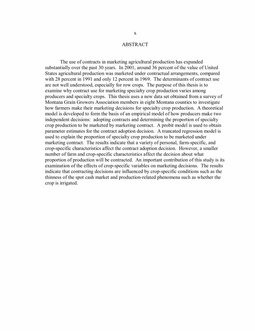
The use of contracts in marketing agricultural production has expanded substantially over the past 30 years. In 2001, around 36 percent of the value of United States agricultural production was marketed under contractual arrangements, compared with 28 percent in 1991 and only 12 percent in 1969. The determinants of contract use are not well understood, especially for row crops. The purpose of this thesis is to examine why contract use for marketing specialty crop production varies among producers and specialty crops. This thesis uses a new data set obtained from a survey of Montana Grain Growers Association members in eight Montana counties to investigate how farmers make their marketing decisions for specialty crop production. A theoretical model is developed to form the basis of an empirical model of how producers make two independent decisions: adopting contracts and determining the proportion of specialty crop production to be marketed by marketing contract. A probit model is used to obtain parameter estimates for the contract adoption decision. A truncated regression model is used to explain the proportion of specialty crop production to be marketed under marketing contract. The results indicate that a variety of personal, farm-specific, and crop-specific characteristics affect the contract adoption decision. However, a smaller number of farm and crop-specific characteristics affect the decision about what proportion of production will be contracted. An important contribution of this study is its examination of the effects of crop-specific variables on marketing decisions. The results indicate that contracting decisions are influenced by crop-specific conditions such as the thinness of the spot cash market and production-related phenomena such as whether the crop is irrigated.

1

CHAPTER 1

INTRODUCTION

The purpose of this study is to understand why the use of contracts varies across

individual producers and individual crops by examining the marketing of specialty crops

by Montana producers. The determinants of marketing channel use and the use of

contracts in general are not well understood. This study examines how producers make

marketing decisions and how a variety of characteristics affect the use of contracts for the

marketing of agricultural production. An improved understanding of producer behavior

and the characteristics that influence the use of contracts enhances the ability of policy

makers to provide information and programs that would improve economic welfare and

economic efficiency. It also facilitates the ability of producers to make effective

marketing decisions.

The objective of this research is to advance our understanding of producer

behavior in general and why certain crops are marketed more frequently with contracts

over other methods such as the spot cash market. Previous studies in this research area

have focused on the effects of personal and farm-specific characteristics on marketing

decisions. The effects of personal characteristics such as producer age, experience,

education, and use of various pricing information sources have been examined in

previous studies. Farm-specific characteristics have been accounted for by variables

measuring crop specialization, gross farm income, debt-to-asset ratios, use of futures,

options, and insurance, and use of various inputs. This study incorporates similar

2 variables to capture the effects of personal and farm-specific characteristics, but also

investigates the effect of a third category of crop-specific characteristics through the use

of variables such as crop-specific dummy variables, distance to the market for delivery of

production, and the investment of resources into the production process of a particular

crop.

The effects of the three categories of characteristics on marketing decisions are

examined in the context of a model for the adoption of marketing contracts and the

decision of what proportion of production to contract. The two decisions are modeled in

a utility of profit maximization framework for individual producers and the effects of

specific variables that proxy for the three general categories of characteristics are

modeled independently for each of the two decisions.

This thesis proceeds as follows. Chapter 2 presents background information on

the use of contracts within the agricultural industry. Chapter 3 reviews the theoretical

and empirical literature on contract theory and the determinants of contract use, including

Katchova and Miranda�s (2004) study on the determinants of contract use by corn,

soybean, and wheat producers from which this study draws heavily. Chapter 4 develops

and presents a theoretical model of how producers decide whether to adopt marketing

contracts and what proportion of their production to market with contracts. This model

allows the three general categories of characteristics to influence each marketing decision

independently and therefore several hypotheses were developed from this theoretical

framework and data were collected to test them. Chapter 5 describes the data and the

survey methodology utilized to collect the data. This study examines a new dataset

3 obtained by surveying members of the Montana Grain Growers Association residing in

Montana counties with the highest levels of specialty crop production. Questions for the

survey were drafted to provide variables that proxy for the three general categories of

characteristics important in this study. Two survey forms were collected from each

individual producer. The first survey provided information on the general farming

operation and the second survey provided information for the production of specific

specialty crops. Chapter 6 presents the empirical models used to estimate the effects of

personal, farm-specific, and crop-specific characteristics on both the adoption of

marketing contracts and the contracted proportion of production decision. The inclusion

of crop-specific variables extends previous research and provides new results for crop-

specific characteristics as well as additional insights about the effect of personal and

farm-specific characteristics. In addition, Chapter 6 also presents the results from the

empirical models. Chapter 7 summarizes the major findings of this thesis, the

implications of the results, limitations of the thesis, and possibilities for future research.

4

CHAPTER 2

CONTRACTS IN AMERICAN AGRICULTURE

In economics, the simple activity of exchanging goods and services, whether on

organized exchanges or outside a market setting, is the basic first step in any production

or allocation of resources (Bolton and Dewatripont 2005). The production and sale of

commodities, either crops or livestock, can be broken down into a series of simple

exchanges of goods or services. Although a variety of arrangements between the parties

involved in the exchange may be established, contracting of agricultural production has

become more common and the subject of an increasing area of research.

Spot market or cash sales for crops can be defined as arrangements in the

agricultural industry where farmers sell products directly to the marketing agent or firm

either immediately after harvest or at some other time during the crop year. The key

dimension is that both parts of the exchange occur at the same moment in time, without

any prior agreements about the nature and structure of the transaction. A contract,

generally speaking, is a written or oral agreement between parties that involves an

enforceable promise to do, or to refrain from doing something (Agriculture 1996). In the

context of agricultural production, contracting a series of exchanges can be defined as a

means to coordinate successive stages in a commodity system (Schrader 1986), or as a

mechanism that specifies a stable price or pricing formula in order to provide security to

the producer and buyer involved in the transaction.

5

Economics of Contract Use

Contractual arrangements may be preferred to other marketing mechanisms such

as the spot cash market for many reasons. Contracts may offer any or all of the following

potential benefits to the producer involved in the transaction: reduced income risk,

reduced price risk, improved access to capital and credit, improved efficiency, provision

of inputs, and providing a guarantee that a market exists for the commodity being

produced. The contractor, or buyer, may also enter into contracts for various reasons.

These include controlling the supply of inputs in agricultural production, increasing the

reliability of commodity quality, sharing price risk with producers, increasing the

predictability of costs, improving response to consumer demands and preferences,

expanding or diversifying operations, and ensuring a steady supply of the commodity

from producers.

There are also potential drawbacks or costs of entering into contracts for both

producers and buyers. The costs associated with contracts for agricultural producers

range from the costs of information gathering, searching for a buyer, negotiating with

potential buyers, physically arranging the contractual elements with the buyers, risk of

buyer default, restrictions on input use imposed by the buyer, quality discounts associated

with the contract, and the risk of failure to deliver the crop to the buyer due to unforeseen

circumstances. There are also costs associated with contracts for buyers as well. The

costs of contracting for buyers include the financial commitment to purchase specific

quantities of the crop, a risk of quantity shortfalls if the producer is unable to deliver, and

6 the risks associated with locking in a price that may continue to fluctuate after the

contract is established. Thus, there are both costs and benefits for both parties entering

into contracts and the relative magnitudes of each must be examined by both the producer

and buyer before entering into the contractual arrangement.

Types of Contracts

Two broad categories of contracts, marketing contracts and production contracts,

are most commonly found in American agriculture. Utilizing previous work by

Harwood, Katchova and Miranda (2004) define a marketing contract as an agreement

between a producer and a buyer that sets a price or price formula for a commodity to be

delivered at a later time. Often, in a marketing contract, the farmer or producer of the

commodity retains ownership of the commodity during production, maintains substantial

control over management decisions, and requires limited direction from the contractor or

purchaser of the commodity. Production contracts, however, often specify in detail the

production inputs supplied by the contractor, the quality and quantity of the particular

commodity being produced, and the form of payment or compensation from the

contractor to the producer (Agriculture 1996).

In 2001, around thirty-six percent of the value of United States agricultural

production was produced and/or marketed under contractual arrangements, compared

with twenty-eight percent in 1991 and only twelve percent in 1969 (Agriculture 2004).

The expansion of the use of contractual arrangements has been profound, but also varied

among agricultural commodities. McLeay and Zwart (1998) found that over ninety

7 percent of production in the egg, broiler, processed vegetable, and turkey industries is

marketed using contracts or other forms of vertically integrated channels. In addition,

over the past decade, hog and tobacco production has rapidly moved away from spot

market-oriented transactions to contract production. In 1991-1993 contracts covered only

one-third of livestock production. Now, contracts cover nearly one-half of total livestock

production. In contrast, contracts currently only cover twenty-five percent of crop

production. The type of contract used also varies by industry. Marketing contracts are

used in both crop and livestock marketing. However, production contracts are common

in the livestock sector, but rarely used in the crop sector.

The theoretical and empirical literature examines contract theory, the use of

contracts in different industries, and issues regarding contract adoption, optimal

contracts, and behavior of contracting parties. Empirical applications of theoretical

developments in contracting have been limited in their scope and often relate to specific

issues and problems such as tenancy arrangements used in contract hog production,

sharecropping, or the egg, broiler, and turkey industries (McLeay and Zwart 1998). Early

research on contracts and a large portion of the subsequent contracting literature deals

with issues such as principal-agent theory and the arrangement of incentives, loss of

autonomy, post-contractual opportunism, and other behavioral considerations that

concern legal issues between contracting parties. An important strand of the contracting

literature extends insights on contracting use to sharecropping and tenancy arrangements

in agriculture (Cheung 1969; Stiglitz 1974). These issues are not the focus of this study.

8

Research on the shift in American agriculture from reliance on the spot market to

the now widespread use of contracts was initiated in the early to mid 1980�s. The

expansion of contracting was seen both as a structural change in various markets in the

agricultural industry along with a change in the structure of the internal organization of

the firm (Schrader 1986). Risk mitigation is also a central element of the current increase

in contracting for both producers and buyers of agricultural production. Variability in

prices, weather, and market conditions cause producers, assumed to be risk-averse, to

utilize contracts as a way to reduce risks and to shift risk to the buyer, who is typically

assumed to be risk-neutral. Studies of contracts not related to sharecropping, tenancy, or

strictly risk-related issues widely recognize that contractual production and even vertical

integration is more common with livestock, broilers, turkeys, fruits, vegetables, and dairy

in the United States but less common in grain production (Lajili et al. 1997). Beginning

in the mid to late 1990�s, however, researchers began to examine the causes of shifts

toward contracting in the production of commodities ranging from livestock to grains.

These studies focused on separating marketing practices into categories such as the spot

cash market, forward contracts, and futures/options. Several studies discussed factors

affecting the choice of one marketing practice over another with the overriding

assumption that a �forward contract� is essentially a marketing contract.

As discussed earlier, there are both benefits and costs to contracting for producers

and buyers, and therefore the reasons for contracting specific crops by individual

producers can vary substantially. However, previous studies have focused on specific

reasons for contracting including marketing contracts that reduce price risk (which can be

9 done with other mechanisms such as the futures market in some industries), coordinating

a market for a task such as processing, as a means to try and utilize market power (such

as in the poultry industry), for efficiency gains, and for producers� improved access to

capital.

The dataset utilized in this study involves contracts that serve the purpose of

providing structure for marketing decisions made for the production of specialty crops. A

majority of the contracts utilized in the specialty crop sector are marketing contracts.

Only recently have researchers begun to examine the factors affecting the use of contracts

or the spot cash market for various commodities and individual producers. The main

questions to be investigated are: (a) why certain commodities are dominated by contract-

oriented transactions while others rely upon spot markets, and (b) why, within an

industry, some producers choose to market their production with a contract while others

prefer the spot market. Approximately sixty percent of the value of agricultural

production within the United States is still sold on spot markets, and thus it is important

to try and understand why certain industries and individuals are beginning the transition

away from the spot market to contracted production.

Summary

There are costs and benefits involved in entering into contracts, and the increasing

use of contracts within the agricultural industry has been an area of focus within

economic research over the past two decades. There are two main categories of

contracts, production and marketing, and the use of marketing contracts within grain

10 production has been increasing over the past fifteen years. This study will attempt to

enhance our understanding of why producers of specialty crops utilize marketing

contracts to market their production with an emphasis on trying to understand the specific

characteristics that significantly influence the use of contracts. The next chapter will

review the theoretical and empirical literature on contract theory and the determinants of

contract use.

11

CHAPTER 3

LITERATURE REVIEW

In 1969, Cheung argued that, �every transaction involves a contract.� Since then,

the analysis of contracts has come to occupy a central place in economic theory. Two

primary approaches, principal-agent theory and transactions cost theory, have informed

the analysis of various issues surrounding the concepts of contracting which include

efficient and optimal contract design, characteristics influencing contract use, and other

issues such as post-contractual opportunistic behavior and default.

The economic analysis of contracts in agriculture was initiated in the early

1980�s. Agricultural contracts have been examined in both the theoretical and empirical

literature to determine how issues from general contracting theory, such as efficient and

optimal contract design along with the other issues previously mentioned, affect the use

and design of contracts within the agricultural industry.

This chapter presents a review of contract theory that is relevant to the literature

of agricultural contracts. Both the theoretical and empirical work on the economics of

agricultural contracts will be reviewed to determine the issues most pertinent to the focus

of this study, the use of marketing contracts in the production of specialty crops within

the agricultural industry.

12

Contract Theory

Jensen and Meckling (1976) develop the principal-agent problem in the context of

one or more principals engaging an agent to perform some service on their behalf, and

this transaction involves delegating some decision making authority to the agent. Under

the assumption that both the principal and agent are utility maximizers, they further

develop the principal-agent problem to show how the agent may not always act in the

best interest of the principal and that the principal may undertake actions in an attempt to

provide the agent with behavior-modifying incentives. Holmstrom (1979) showed how

imperfect information can create moral hazard or dysfunctional behavior in the principal-

agent problem which can be alleviated by the investment of resources into monitoring or

other activities. These additional investments, or the creation of additional information

systems to mitigate the moral hazard actions of the agent, can help to improve contracts

between the principal and the agent. Stiglitz (1974) approached agricultural

sharecropping from a principal-agent standpoint, under the assumption that the principal

(landlord) is risk-neutral while the agent (producer) is risk-averse, and the relationship is

modeled to capture the importance of risk sharing in sharecropping contracts. Stiglitz

concluded that the main advantage of a share contract is to reduce the moral hazard

problem in the presence of a risk-averse tenant.

Risk-sharing and the effects of risk preferences among the contracting parties are

standard considerations in principal-agent analyses. Cheung (1969) began his analysis

with risk -verse producers (agents) avoiding risk if the cost of doing so is less than the

13 gain from the risk averted. In the context of agricultural production and marketing,

Hudson and Lusk (2004) extend this insight to claim that, as risk-averse agents,

producers should be willing to give up some income to shift the risk to the buyer of

agricultural production, creating a risk premium. Risk has been analyzed as an important

factor in the production choices made by small farmers for quite some time (Sandmo

1971). The importance of risk is traced to the fact that agricultural producers typically

face considerable production and price risk in their operations and in the various

economic and business environments under which they operate (Hueth and Ligon 1999).

The assumptions of risk preferences for principals and agents along with the role of risk-

sharing and moral hazard reduction in contracts serve as two of the main tools by which

contracts are investigated in principal-agent analyses.

Transactions cost theory often relaxes the assumption of a risk-averse agent and

instead focuses on the costs inherent in every transaction and the incentives these costs

create for both the principal and the agent, regardless of attitudes toward risk. Arrow

(1969) provides a broad definition of transaction costs as, �(the) costs of running the

economic system.� Coase (1937) provided the foundational work of transactions cost

theory through his investigation of why a firm emerges to take on the coordinating tasks

typically left to the price mechanism in the market. He recognized that there are costs to

use the price mechanism. These include costs of discovering what prices are, along with

negotiating and concluding separate contracts for each transaction. Cheung (1969)

extended Coase�s insight by stating that one reason for the existence of different

contractual arrangements stems from differences in transactions costs that are associated

14 with them. Cheung also claimed that transaction costs differ, �because the physical

attributes of input and output differ, because institutional arrangements differ, and

because different sets of stipulations require varying efforts in enforcement and

negotiation.� Williamson (1979; 1981; 1991) extended the work of both Coase and

Cheung by focusing on how the presence of transactions costs significantly affects the

organization of economic activity, and differing transaction costs provide incentives to

utilize various institutions for transactions from the open market to internal organization

of vertical coordination in a firm.

Klein, Crawford, and Alchian (1978) investigated one particular transaction cost

of using the market system: post-contractual opportunism that arises through the pursuit

of quasi-rents which are created after a specialized investment into the production of the

particular asset to be exchanged. They conclude that as the amount of asset-specific

investment increases, quasi-rents increase and, accordingly, the threat of reneging on the

contract by the buyer increases. Alternative arrangements through contracting or vertical

integration can be undertaken to reduce the possibility of post-contractual opportunistic

behavior. Transactions costs can be defined by the investments undertaken in post-

contractual behavior or the prevention of opportunistic behavior. Therefore, transactions

cost theory focuses on monitoring costs, enforcement costs, and the costs of the post-

contractual opportunistic behavior as defined by Klein, Crawford, and Alchian. Leffler

and Rucker (1991) extend Klein, Crawford, and Alchian�s insight by demonstrating that

individuals and firms are shown to develop institutions and contractual arrangements to

minimize dissipation from transaction costs. They state that the specific nature of the

15 transaction costs can be related to the physical properties of the goods being exchanged

and the characteristics of the particular buyers and sellers.

Principal-agent theory and transactions cost theory are often at odds with one

another in the assumptions that they place on the behavior and incentives of individuals

involved in a transaction and the nature of the relationship among those individuals.

Hudson and Lusk (2004) distinguish principal-agent theory from transactions cost theory

by stating that standard principal-agent models assume contracts are costless to write and

complete, while transactions cost theory assumes that contracts are both costly to write

and costly to fulfill. However, recent works by Ackerberg and Botticini (2002) along

with Hudson and Lusk (2004), have approached contracting issues by investigating the

effects of both risk and transactions costs in a contractual relationship and have presented

evidence that both are important in explaining various aspects of contracting.

Empirical Literature

Contract theory has been applied to various aspects of the agricultural industry

and has served as the rationale for empirical investigations of various issues concerning

forms of agricultural organization and agricultural contracting relationships1. The

1 Numerous applications of contract theory to agricultural applications will not be addressed within the context of this thesis. Input and management control, moral hazard, and efficient contracts within broiler and overall livestock production contracts in the agricultural industry are investigated by Goodhue (1999), Ward et al. (2000), Morrison-Paul et al. (2004), Vukina and Dubois (2004), and Vukina and Levy (2004). Cheung (1969), Stiglitz (1974) and others perform their analyses of contracting with respect to a specific sharecropping application. Issues such as moral hazard, risk sharing, imperfect capital markets and the overall function of contracts are investigated by Allen and Lueck (1999), Ackerberg and Botticini (2000) and others. Applications of optimal risk and various contractual provisions regarding quality, identity preservation, multitasking, and policing mechanisms are examined in an optimal contract framework with a specific application to fresh produce include work by Hueth and Ligon (1999), Ligon (2002; 2003), Wolf et

16 insights of both principal-agent and transactions cost theories are relevant in the analysis

of whether or not marketing contracts are utilized for the production of agricultural

commodities. The overriding questions are what characteristics influence individual

producers to use marketing contracts and what characteristics of crops make them more

likely to be subject to marketing contracts. These issues have been investigated in the

empirical literature through both principal-agent and transactions cost approaches.

The rationale for marketing contract adoption by agricultural producers is

supported in various ways from contract theory. Principal-agent theory identified the

importance of risk-reduction in contracting relationships and transactions cost theory

highlighted the importance of transactions cost minimization in contracting. Extensions

of both approaches can help to explain the use of marketing contracts for agricultural

commodities. Schrader (1986) examined the use of agricultural marketing contracts to

coordinate successive stages of agricultural production, as opposed to open production

and pure market exchange. He identified four reasons for coordinating agricultural

production by non-market means: to increase efficiency, to gain market advantage, to

reduce uncertainty, and to obtain or reduce the cost of financing.

Fletcher and Terza (1986) provided an empirical application of contract theory by

utilizing principal-agent theory to investigate how risk-averse farmers deal with

increasing risk from cost inflation and higher variability in commodity prices. Fletcher

and Terza, along with McLeay and Zwart (1998), tried to identify the farmers�

characteristics that make them most likely to diversify in response to increasing risk, al. (2001), and Hueth and Melkonyan (2004). Other applications of contract theory exist and are not considered within the contexts of this thesis.

17 along with the characteristics of industries that support the use of particular marketing

channels. Edelman, Schmiesing, and Olsen (1990) identify income and price variability

stemming from the trend toward less government involvement in agricultural programs to

motivate an investigation into the specific characteristics of producers that could be

targeted with information and management assistance to deal with the deregulated

agricultural environment.

Shapiro and Brorsen (1988), Asplund, Forster, and Stout (1989), Goodwin and

Schroeder (1994), and Musser, Patrick and Eckman (1996) all utilized portfolio theory to

show that, with increasing price and income risk, farmers should be utilizing futures

markets or forward contracts. However, fewer producers utilize such risk-reducing

mechanisms than portfolio theory predicts (Shapiro and Brorsen 1988). All of the

portfolio theory-based empirical applications investigate producer characteristics that

influence the use of forward contracts or hedging with the futures market. In these

applications, the authors attempt to identify characteristics that might be responsible for

why hedging and forward contracts are used less than the efficient rate predicted from

portfolio theory. Sartwelle et al. (2000) along with Katchova and Miranda (2004)

extended portfolio models to incorporate an analysis of how personal and farm

characteristics affect pre and post-harvest marketing practices with separate decisions for

contract adoption, quantity contracted, frequency of contracting, and contract type.

Even though the empirical literature utilizes various theoretical assumptions to

investigate the characteristics that influence the use of contracts, all of the studies utilized

survey data from a variety of sources. All of the most relevant empirical studies utilized

18 survey data with maximum likelihood econometric estimation for limited dependent

variables, and differences only come in the use of econometric method utilized. See

Appendix A for a table of the various methods utilized and key findings in the empirical

literature.

The empirical estimation techniques identified in Appendix A are utilized to

obtain estimates on the effects of various characteristics influencing the use of contracts

for the marketing of agricultural production. The decision-making process of producers

is modeled in various ways in the empirical literature. Edelman, Schmiesing, and Olsen

(1990), McLeay and Zwart (1998), and Sartwelle et al. (2000) each develop general

models of producer decisions that investigate specific factors and characteristics

influencing the choice of marketing practices. Shapiro and Brorsen, along with Asplund,

Forster, and Stout, model the decision-making process in a technology adoption

framework where specific producer characteristics influence whether or not a producer is

likely to adopt a new technology, such as a marketing contract. Fletcher and Terza,

Goodwin and Schroeder, and Katchova and Miranda model the decision-making process

as a utility maximization problem for producers. Fletcher and Terza assume that

producers maximize utility in general and develop assumptions about the effects of

specific characteristics from that foundation, while both Goodwin and Schroeder and

Katchova and Miranda assume that producers maximize the expected utility of profits.

All of the above studies investigate the effects of characteristics on the use of marketing

contracts and other marketing mechanisms in the agricultural production process, but the

19 various modeling techniques and assumptions lead to slightly different estimation

mechanics and predicted effects.

In addition to various models and assumptions utilized throughout the empirical

literature, the specific characteristics and factors influencing producers� use of marketing

contracts vary widely. Specific characteristics of individual producers influence how

individuals deal with risk, along with how individuals deal with transactions costs that

exist for use of particular marketing mechanisms. The characteristics that influenced

marketing decisions and the use of forward contracts in the empirical literature fall into

three categories: personal characteristics (descriptive characteristics, preferences,

opinions, actions, etc.) of the producer, farm-specific characteristics, and crop/industry

characteristics.

The characteristics most thoroughly investigated in the empirical literature are the

personal characteristics of individual producers. Age and experience are two of the most

frequently utilized personal characteristics. However, Asplund, Forster, and Stout and

others have found age and experience are highly correlated and therefore empirical

investigations typically utilize either age or experience and not both. Although some

studies found that age and experience are not significant, Shapiro and Brorsen reported

that more experienced producers are less likely to hedge and use other price risk-reducing

strategies such as forward contracting, a finding consistent with results reported by

Asplund, Forster, and Stout, Sartwelle et al., and Goodwin and Schroeder2. Katchova

2 Fletcher and Terza and Musser, Patrick, and Eckman used age as a proxy for experience and they expected that producers with more experience (older) have shorter planning horizons and thus younger farmers would be more likely to recover the costs associated with the adoption of forward pricing

20 and Miranda, however, reported that older farmers are more likely to adopt forward

contracting.

The effect of education on the use of contracting and other marketing strategies

has also been examined. Fletcher and Terza, Goodwin and Schroeder, Musser, Patrick,

and Eckman, and Katchova and Miranda all found that increased education increased the

use of forward contracts and other forward pricing mechanisms3. Similarly, Fletcher and

Terza, Asplund, Forster, and Stout, Goodwin and Schroeder, and Katchova and Miranda

provide evidence that producers using farm associations and attending educational

seminars are more likely to adopt marketing contracts. In contrast, Shapiro and Brorsen

found that highly educated producers were less likely to participate in forward pricing

marketing mechanisms4.

The use of crop insurance and producer risk preferences are two additional

personal characteristics examined in the empirical literature. Goodwin and Schroeder

and Sartwelle et al. reported that producers who use crop insurance also were more likely

to use forward contracts, but Katchova and Miranda found just the opposite5. Risk-

related variables are also widely used, but few empirical studies find them to be

significant in the decision of whether or not to use forward contracts. Goodwin and

mechanisms. Likewise, from a technology adoption standpoint, Asplund, Forster, and Stout expected that adopters of innovation are likely to be younger. 3 Technology adoption theory, according to Fletcher and Terza and Goodwin and Schroeder, provides the rationale that highly educated producers are expected to have advantages in using new technology and are thus more likely to adopt technology. Likewise, Musser, Patrick, and Eckman utilize human capital theory to argue that a higher level of human capital attained through education facilitates the successful use of forward pricing strategies. 4 Shapiro and Brorsen reported that more educated producers are more likely to be less risk-averse, and thus less likely to adopt forward contracts to reduce price and income risk. 5 Goodwin and Schroeder and Sartwelle et al. suggest that insurance and forward contracting are complements, but Katchova and Miranda consider them to be substitutes.

21 Schroeder found that producers with a preference for risk were more likely to use forward

pricing mechanisms, while Musser, Patrick, and Eckman found that producers more

concerned about the potential for losses were most likely to use forward contracts. Thus,

the empirical evidence concerning the effects of risk is mixed. The empirical results

obtained with measures of risk must be viewed with caution, however, as mechanisms for

measuring risk and incorporating its effects into a decision-making model were not

consistent across empirical studies.

Farm-specific characteristics are also utilized widely in the empirical literature.

Income-related variables and variables concerning farm/operation acreage are some of

the most commonly used variables to proxy for farm-specific characteristics6. Asplund,

Forster, and Stout, Edelman, Schmiesing, and Olsen, and Katchova and Miranda all

present evidence that farms with higher incomes (gross sales, gross receipts, gross farm

income) are more likely to use forward contracts. Musser, Patrick, and Eckman,

however, propose that lower farm income leads to increased use of forward contracts, but

only for short-term corn marketing. Their empirical results concerning farm size

characteristics supported the hypothesis that larger farmers were more likely to use

forward contracts, thus also providing support for the economies of size argument in

terms of farm acreage7.

6 Both farm income and acreage are utilized to proxy for �economies of size� that may exist in the farming operation with reference to forward contract use. Asplund, Forster, and Stout, drawing upon transactions cost theory to explain economies of size in relation to income, argue that a minimum level of gross sales may be required to justify the time, effort, and expense incurred from forward contracting. Sartwelle et al. also argue that larger farms (in acreage) have lower per-unit costs than smaller farms in terms of learning how to use marketing tools and collecting marketing information. 7 Fletcher and Terza, Shapiro and Brorsen, Goodwin and Schroeder, McLeay and Zwart, and Sartwelle et al. all report that forward contract use increases as farm acreage increases.

22

Some empirical studies also included measures of how reliant on a particular crop

farm operators are through measures of specialization or dependence. Edelman,

Schmiesing, and Olsen, Sartwelle et al., and Katchova and Miranda all include measures

of specialization, defined as the percentage of overall income coming from the particular

crop of interest. All of the studies report that as the percentage of income from a

particular crop increases so does the use of forward contracts. McLeay and Zwart also

include a measure of dependence based on the percentage of the total effective crop area

that the relevant crop utilized. They report that as the farm�s dependence on a crop

increases, so does the likelihood of contracting8.

Some empirical studies included measures of financial leverage, typically in the

form of debt-to-asset ratios9. Shapiro and Brorsen, Asplund, Forster, and Stout, Edelman,

Schmiesing, and Olsen, Goodwin and Schroeder, and Katchova and Miranda all report

that higher leveraged producers are more likely to adopt forward marketing contracts.

Other variables are also utilized in some studies. Goodwin and Schroeder and

McLeay and Zwart report that farm operations with larger investments in inputs and

physical capital (as measured by input intensities) are more likely to utilize forward

pricing mechanisms10. Variables accounting for the presence of storage facilities on the

farm provided mixed results. Fletcher and Terza find that the presence of storage

8 McLeay and Zwart offer the rationale that as the level of dependence on a product increases, so does the exposure to falling prices and therefore contracting is more likely to avoid sales risk. This theory of risk-reduction can also be related to the income specialization variables utilized by Edelman, Schmiesing, and Olsen, Sartwelle et al. and Katchova and Miranda. 9 The argument concerning financial leverage is based on theory described by Asplund, Forster, and Stout. They argue that highly leveraged producers utilize forward contracts to reduce downside price risk. Also, farm lenders require highly leveraged producers to use forward pricing mechanisms. 10 Goodwin and Schroeder state that firms with a larger investment in inputs face greater exposure to risk and therefore are more likely to utilize forward contracts to deal with the increased risk.

23 increases the use of forward contracts, but Sartwelle et al. finding that farmers without

storage are more likely to forward contract11.

After personal and farm-specific characteristics, crop/industry characteristics have

been utilized much less in the empirical literature. McLeay and Zwart investigate

specific crop characteristics that influenced the adoption of contracts. They find that

traditional crops and crops whose markets are not influenced by international market

conditions are less likely to be contracted12. Sartwelle et al. find that being near a major

grain demand center significantly increases the use of futures and options but has no

effect on forward contracting13.

Summary

Contract theory has been shaped around the two theoretical strands of principal-

agent theory and transactions cost theory. From these two theoretical approaches, issues

of risk-reduction and transactions cost mitigation emerged into the literature surrounding

various contracting relationships and issues. Contract theory has had a variety of

applications in agriculture, one of which is the effect of risk and transactions cost on the

11 Although Fletcher and Terza offer no rationale for their results, Sartwelle et al. provides a transactions cost justification. Farmers with storage can retain ownership of their crop after harvest to try and benefit from post-harvest price increases, and farmers without storage must be more aggressive pre-harvest marketers. 12 McLeay and Zwart describe how crops only sold domestically may have a free market with a built-in stabilizing or risk-adjustment aspect. Also, with respect to traditional crops, producers may have accumulated production knowledge and therefore production and marketing requires less human capital and leads to more market sales. The prevalence and availability of government payments may also reduce the need for marketing contracts among traditional crops. 13 Sartwelle et al. hypothesize that being near a grain demand center would increase the use of forward contracts, presumably due to lower transactions cost in finding and dealing with buyers, but the opposite effect could also exist because producers who are farther away face increased risk of not finding a buyer and therefore would be more likely to use a forward contract.

24 choice of utilizing a contract for the marketing of agricultural production. Various

characteristics of producers and commodities are examined throughout the empirical

literature. Drawing upon the econometric methodology utilized throughout various

empirical applications, this study will investigate the effects of characteristics such as

farm size, specialization, leverage, but also additional producer and commodity-specific

characteristics. These efforts will attempt to identify those characteristics that

significantly affect the use of various marketing mechanisms for the production of

specialty crops such as malting barley, mustard seed, safflower, flax, lentils, canola and

dry edible peas. In the next chapter, theories are presented to develop hypotheses about

the specific effects of the various characteristics of which data has been obtained for the

purposes of this study.

23

CHAPTER 4

THEORETICAL MODELS Specialty crop producers make many decisions concerning production and

marketing of these crops. Producers of more common small grains such as wheat or

barley can utilize a variety of marketing mechanisms ranging from marketing contracts

and the spot cash market to futures and options. Specialty crops, however, do not have

futures or options markets and thus specialty crop producers generally choose between

the spot cash market or marketing contracts in selling their production, although some

specialty crops may be utilized on the farm and ranching operation for livestock feed.

The purpose of this chapter is to investigate the economic decisions involved in specialty

crop production and to identify the factors or characteristics that influence the producer�s

marketing decisions. The theoretical framework used to examine these issues is one in

which producers are assumed to maximize their expected utility of profits from the

production and marketing of specialty crop production.

Goodwin and Schroeder (1994) develop a one-step expected utility maximization

model to investigate the decision of how producers market agricultural production. They

assume that the adoption of marketing contracts has previously been made and the

subsequent decision of interest is what proportion of agricultural production to market

with marketing contracts. Katchova and Miranda (2004) extend Goodwin and

Schroeder�s model to a two-step environment in which decisions about marketing

agricultural production are conditional upon the decision to adopt marketing contracts.

24

This study will extend Katchova and Miranda�s two-step theoretical framework for a

specialty crop producer maximizing the expected utility of profits by modeling the

decision to adopt marketing contracts and the decision about what proportion of specialty

crop production to market with marketing contracts.

The Expected Utility of Profits Model

A specialty crop producer�s marketing decision is examined under the assumption

that the decision to plant the specialty crop has been made and that a producer�s

subsequent decision is how to market the resulting output. The outcome of the

producer�s marketing decision is uncertain. However, producers are assumed to market

specialty crops in order to maximize their expected utility of profits. In addition,

marketing contracts are assumed to be available; that is, buyers of specialty crops are

willing to offer marketing contracts to producers.

A marketing contract provides a producer with a specific, and often a guaranteed,

price for the specialty crop production based on a variety of factors14. In adopting

marketing contracts, however, producers must also incur costs associated with their

adoption. The fixed and variable costs associated with marketing contracts could range

from costs of information gathering, searching for a buyer, negotiating with potential

buyers, and arranging the contractual elements with the buyer. The spot cash market also

14 There are a variety of different types of price guarantees. Examples of price guarantees include a set price based upon the spot cash market price at the time of signing, a pre-determined price negotiated by buyer and seller alike, and a price that is determined solely by the buyer at the time of the signing.

25

transmits a price to the specialty crop producer. This study assumes that, ex ante, the

spot cash market price is distributed as a random variable.

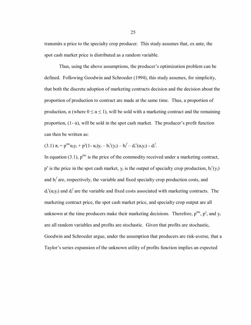
Thus, using the above assumptions, the producer�s optimization problem can be

defined. Following Goodwin and Schroeder (1994), this study assumes, for simplicity,

that both the discrete adoption of marketing contracts decision and the decision about the

proportion of production to contract are made at the same time. Thus, a proportion of

production, α (where 0 ≤ α ≤ 1), will be sold with a marketing contract and the remaining

proportion, (1- α), will be sold in the spot cash market. The producer�s profit function

can then be written as:

(3.1) πi = pmcαiyi + ps(1- αi)yi � biv(yi) � bi

f � div(αiyi) - di

f.

In equation (3.1), pmc is the price of the commodity received under a marketing contract,

ps is the price in the spot cash market, yi is the output of specialty crop production, biv(yi)

and bif are, respectively, the variable and fixed specialty crop production costs, and

div(αiyi) and di

f are the variable and fixed costs associated with marketing contracts. The

marketing contract price, the spot cash market price, and specialty crop output are all

unknown at the time producers make their marketing decisions. Therefore, pmc, ps, and yi

are all random variables and profits are stochastic. Given that profits are stochastic,

Goodwin and Schroeder argue, under the assumption that producers are risk-averse, that a

Taylor�s series expansion of the unknown utility of profits function implies an expected

26

utility of profits maximization where the producer�s profit function can be decomposed

into a set of observable factors related to its mean and variance15.

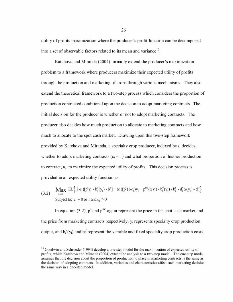
Katchova and Miranda (2004) formally extend the producer�s maximization

problem to a framework where producers maximize their expected utility of profits

through the production and marketing of crops through various mechanisms. They also

extend the theoretical framework to a two-step process which considers the proportion of

production contracted conditional upon the decision to adopt marketing contracts. The

initial decision for the producer is whether or not to adopt marketing contracts. The

producer also decides how much production to allocate to marketing contracts and how

much to allocate to the spot cash market. Drawing upon this two-step framework

provided by Katchova and Miranda, a specialty crop producer, indexed by i, decides

whether to adopt marketing contracts (ci = 1) and what proportion of his/her production

to contract, αi, to maximize the expected utility of profits. This decision process is

provided in an expected utility function as:

(3.2) { }

i i

s v f s mc v f v fi i i i i i i i i i i i i i i i i

c ,

i i

EU (1-c )[p y - b (y ) - b ] + (c )[p (1- )y + p ( y ) - b (y ) - b - d ( y ) - d ]

Subject to: c = 0 or 1 and > 0

Maxα

α α α

α

In equation (3.2), ps and pmc again represent the price in the spot cash market and

the price from marketing contracts respectively, yi represents specialty crop production

output, and biv(yi) and bi

f represent the variable and fixed specialty crop production costs.

15 Goodwin and Schroeder (1994) develop a one-step model for the maximization of expected utility of profits, which Katchova and Miranda (2004) extend the analysis to a two-step model. The one-step model assumes that the decision about the proportion of production to place in marketing contracts is the same as the decision of adopting contracts. In addition, variables and characteristics affect each marketing decision the same way in a one-step model.

27

In addition, ci = 0 indicates the decision not to adopt marketing contracts and is

associated with the first term in the discrete maximization operation, and ci = 1 indicates

the adoption of marketing contracts and is associated with the second term. The costs

associated with marketing contracts, div(αiyi) and di

f, are only incurred if the specialty

crop producer decides to adopt contracts and are therefore only included in the second

term of the optimization problem. Specialty crop producers therefore compare the

benefits of changes in the price distribution associated with marketing contracts with the

costs of entering into the marketing contracts. The producers then compare the expected

utility of profits from adopting marketing contracts for a utility-maximizing proportion of

their specialty crop production to the expected utility of profits utilizing only the spot

cash market and its distribution of prices. Producers will adopt a marketing contract if

the expected utility of profits from using a marketing contract and marketing an optimal

proportion of their production with contracts exceeds the expected utility of profits from

using only the spot cash market.

A Taylor�s series expansion of equation (3.2)�s expected utility of profits

function, similar to that of Goodwin and Schroeder (1994), can be applied to this model

to yield expressions relating producer�s choices of adoption (ci) to zi, a set of observable

personal, farm-specific, and crop-specific characteristics. In addition, the model allows

the producer�s choice of the proportion of his/her production to contract (αi) to be related

to a set of the same or different characteristics, xi.

Maximizing the expected utility of profits therefore yields an expression relating a

producer�s decision of whether or not to adopt a marketing contract, represented by ci, to

28

a matrix of observable personal, farm, and crop characteristics (zi). Formally, ci = h(γ′zi,

εci), where γ is a parameter vector and εci is the error term that represents unmeasured

factors relating to adoption. Also, this model allows for either the same or a different set

of observable personal and farm characteristics, xi, to be related to the producer�s

decision of what proportion of their specialty crop to contract (αi). Thus, αi = gα(βα′xi, εαi)

where βα is a parameter vector and the error term, εαi, represents unmeasured factors

relating to the decision of what proportion to contract. This framework allows some

characteristics to affect both the adoption and the proportion of production contracted

decisions in the same or different ways and it also allows some characteristics to only

enter one decision or the other.

Empirical Application of Theoretical Model

Within this theoretical framework, this study will utilize three general categories

of characteristics: personal characteristics, farm-specific characteristics, and crop-

specific characteristics. Goodwin and Schroeder, Katchova and Miranda, and others all

utilize two general categories of characteristics, personal and farm-specific, to model

producers� marketing decisions. Personal characteristics used in prior studies range from

producer age, experience, education, and use of various pricing information sources.

Farm-specific characteristics include measures of crop specialization, gross farm income,

debt-to asset ratios, use of futures, options, and insurance, and use of various inputs. This

study incorporates specific and varied farm and personal characteristics as well as a third

general category of characteristics related to crop-specific characteristics. Crop-specific

29

characteristics are included to attempt to explain differences in the use of marketing

contracts and spot markets among specific specialty crops or categories of specialty

crops. Hypotheses are developed about the effect particular producer, farm-specific, and

crop-specific characteristics have on the decision to adopt contracts along with the

decision of what proportion of production to contract.

The effects of all three categories of characteristics (personal, farm-specific, and

crop-specific) on the adoption and use of marketing contracts by individual producers are

examined under the assumption that producers are risk-averse. Although the assumption

that producers are risk-averse is common in previous research (Shapiro and Brorsen

1988; Goodwin and Schroeder 1994; Musser et al. 1996; McLeay and Zwart 1998;

Sartwelle et al. 2000; Katchova and Miranda 2004), accounting for possible changes in

risk preferences is difficult because risk preferences are unknown and unobservable.

Therefore, addressing risk-aversion and the effects of characteristics on a producer�s

unknown preference for risk is problematic. In addition, the production of specialty

crops can be viewed as diversifying a farm operation from the production of traditional

crops, but whether or not the production of specialty crops necessarily represents income

diversification is unclear (Johnson and Tefertiller 1964).

Personal Characteristics Producer-specific personal characteristics such as producer age and experience,

human capital accumulation through education, and the adoption of technologies such as

computers in general and for use in various tasks such as bookkeeping may explain why

30

some producers utilize marketing contracts and others do not. As a producer�s level of

experience with a specific market increase, the producer�s familiarity with and ability to

effectively utilize a spot cash market for a specific crop may also increase, and therefore

the use of marketing contracts is potentially inversely related to experience. However,

younger farmers may have less equity and less to lose from taking risks along with a

longer planning horizon over which to recover costs and losses from risks, and therefore

more experienced producers could be considered more risk-averse than younger

producers and experience would be positively related to the use of marketing contracts.

Thus, the expectation for the effect of experience on marketing contract adoption and the

proportion of production contracted is unclear.

Producers with more human capital have lower costs of understanding and

interpreting the terms of the marketing contracts and are therefore more likely to adopt

marketing contracts and utilize contracts for a larger proportion of their production.

Thus, producers with higher levels of education, such as undergraduate or graduate

college degrees, are hypothesized to be more likely to adopt marketing contracts.

However, producers with higher levels of education may also be less risk-averse and less

likely to utilize contracts or contract a lower proportion of specialty crop production

leaving the effects of education ambiguous.

A producer who adopts other technologies, such as a computer, and utilizes the

new technologies within his/her farming operation through tasks such as bookkeeping

with a computer may be more likely to adopt other technologies in the farming operation.

If marketing contracts can be considered a form of new technology which the producer

31

can adopt, then producers who adopt other forms of technology such as utilizing

computers for bookkeeping will be more likely to adopt marketing contracts as well.

Farm-Specific Characteristics

Farm-specific characteristics may also influence whether or not producers adopt

marketing contracts as well as the proportion of production which is marketed with

marketing contracts. Farm-specific characteristics include farm size, gross farm

revenues, whether or not livestock sales are a part of farm revenues, whether or not

additional income for the farm comes from off-farm sources, and general regional

geographic characteristics.

Producers operating a large farm, in terms of either acres or gross farm income,

may have economies of size in the ability to spread the costs incurred from contracting

over a large number of acres or a large amount of gross farm income. Therefore, farm

size and gross farm income may both be positively related to the adoption of marketing

contracts and would lead to an increased proportion of production marketed with

marketing contracts. However, as gross farm income increases, producers may become

less-risk-averse and thus both marketing decisions may be negatively related to gross

farm income. Thus, the effect of gross farm income on the use of contracts is uncertain.

Livestock sales and off-farm income can be viewed as a proxy for enterprise

diversification. Diversified farms have alternative sources to manage risk through off-

farm income or the sale of commodities other than the crop of interest. Therefore,

producers of a diversified operation may be less risk-averse than non-diversified

32

producers with respect to marketing specialty crop production, and thus more willing to

utilize the spot cash market and to contract a lower proportion of production. Also,

producers of more diversified operations have less time to spend on the marketing of

specialty crops and may be unable to invest the time and energy into searching for and

learning the methodology behind utilizing marketing contracts and would therefore be

more likely to use the spot cash market.

Geographic characteristics may also affect contracting decisions. If there are

regional characteristics that are unobserved which influence an individual producer�s use

of marketing contracts, regional dummy variables could help capture the unobserved

influences. Regional variables also capture unknown, random characteristics that affect a

producer�s expectation of the yield for a particular crop. Yield expectations are assumed

to influence the proportion of production a producer is willing to contract. Regional

variables may capture random characteristics that affect yield expectations.

Crop-Specific Characteristics

Examples of crop specific characteristics include whether or not the specialty crop

is an oilseed or a crop used for livestock feed purposes, whether the crop is irrigated, and

the distance from the buyer to the delivery point for the specialty crop production. Crops

that have multiple uses in terms of the markets available to deliver the production may be

less likely to adopt marketing contracts. For instance, a crop that can be used as feed for

livestock may be marketed to a buyer for processing of the crop, used on the farm or

ranch operation for livestock feed in the operation, or sold to a different buyer in the

33

market for livestock feed. This multi-faceted or multi-use crop would be expected to be

associated with a lower proportion of production contracted due to the number of uses

and markets available for its marketing. Crop-specific variables may also capture the

effects of unknown, random characteristics that influence crop yields. As with regional

variables, crop-specific variables that affect a producer�s expectation of crop yield are

directly related to the producer�s decision of what proportion of production to contract.

The variability in yield of specialty crop production and buyer preferences for

specific qualities of a specialty crop may be identifiable in whether or not the specialty

crop is irrigated. There is typically less variability in production from irrigated crops,

and therefore the risk of defaulting on a marketing contract decreases, leading to a higher

proportion of production contracted. Buyers of specialty crops may want to secure a

higher proportion of irrigated specialty crop production to ensure a predictable supply of

the specialty crop. In addition, irrigated specialty crop production may also be more

consistent in quality which is a desirable attribute to buyers as well. Irrigated crops are,

therefore, likely to be contracted more frequently and in higher proportions than non-

irrigated crops.

The distance from the producer�s farm to the delivery point or buyer of the

specialty crop production may have conflicting effects. From a transaction cost

perspective, the costs of delivery will be higher as the distance from the buyer increases

and therefore producers would be expected to cover the additional costs with price risk-

reducing mechanisms such as marketing contracts. However, the relevant distance

measure is the distance between the market for specialty crop production sold under

34

marketing contract and the market for production sold in the spot cash market. As the

relative distance decreases for production marketed with marketing contracts compared to

the spot cash market, transportation costs are relatively lower and therefore marketing

contracts will be utilized more frequently and for a higher proportion of production.

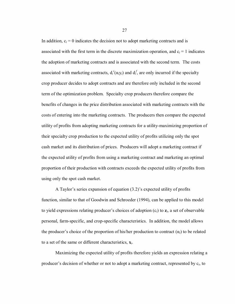
Empirical Contract Adoption and

Proportion of Production Contracted Decisions

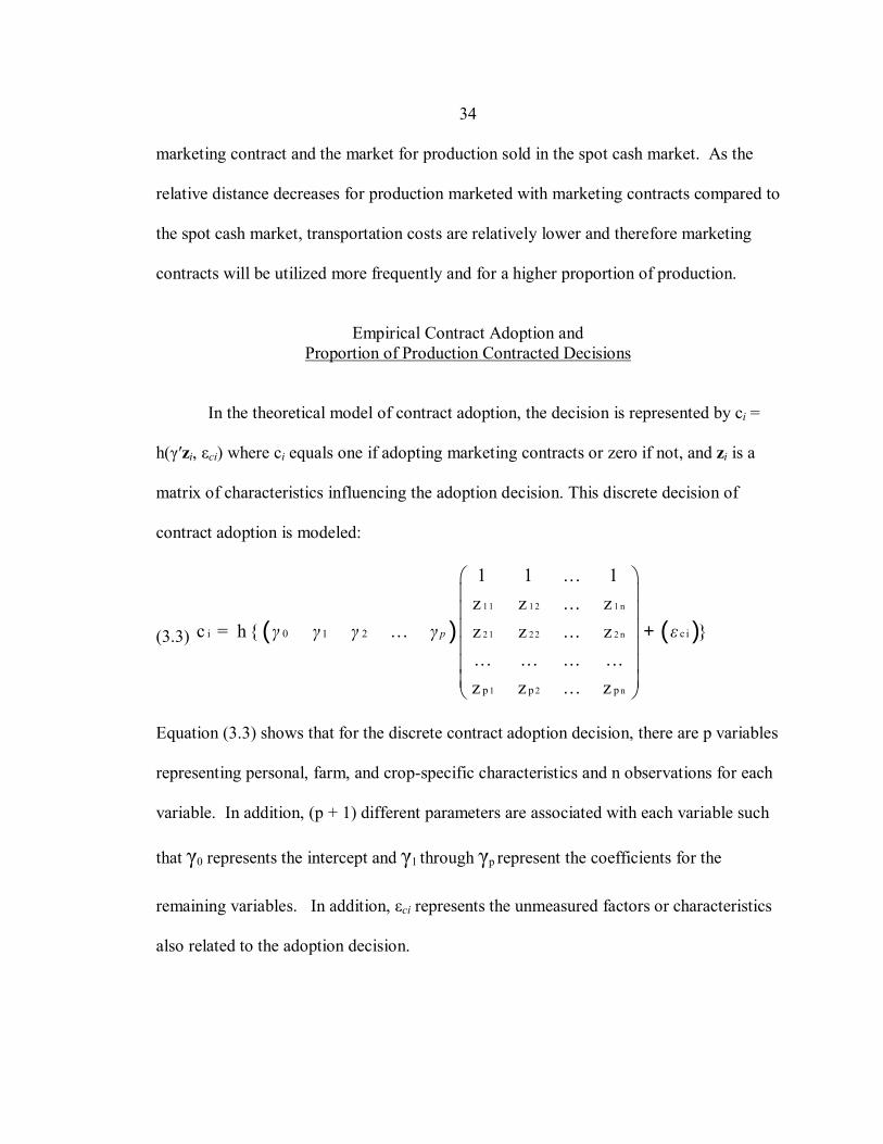
In the theoretical model of contract adoption, the decision is represented by ci =

h(γ′zi, εci) where ci equals one if adopting marketing contracts or zero if not, and zi is a

matrix of characteristics influencing the adoption decision. This discrete decision of

contract adoption is modeled:

(3.3) ( ) ( )1 1 1 2 1 n

2 1 2 2 2 n

1 2 n

i 0 1 2 c i

p p p

1 1 .. . 1z z ... z

c = h { .. . }z z ... z.. . .. . ... . ..z z .. . z

pγ γ γ γ ε

+

Equation (3.3) shows that for the discrete contract adoption decision, there are p variables

representing personal, farm, and crop-specific characteristics and n observations for each

variable. In addition, (p + 1) different parameters are associated with each variable such

that γ0 represents the intercept and γ1 through γp represent the coefficients for the

remaining variables. In addition, εci represents the unmeasured factors or characteristics

also related to the adoption decision.

35

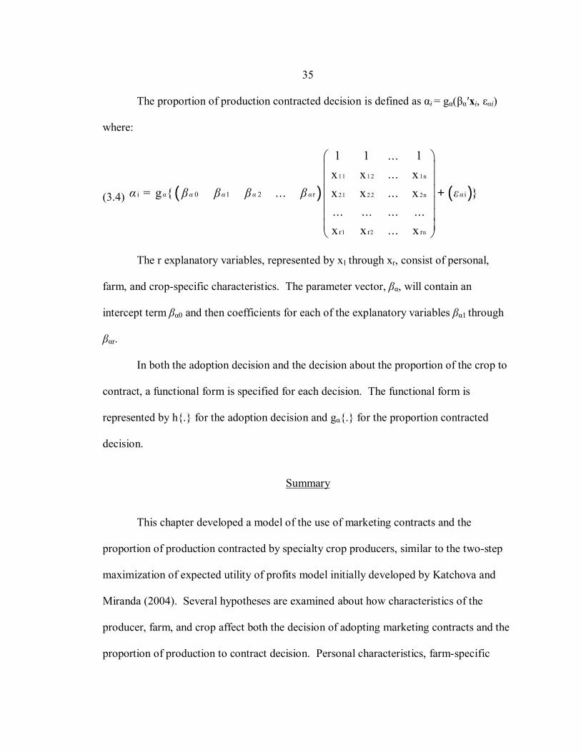
The proportion of production contracted decision is defined as αi = gα(βα′xi, εαi)

where:

(3.4) ( ) ( )11 1 2 1n

21 2 2 2n

1 2 n

i 0 1 2 r i

r r r

1 1 ... 1x x ... x

= g { ... }x x ... x... ... ... ...x x ... x

α α α α α αα β β β β ε

+

The r explanatory variables, represented by x1 through xr, consist of personal,

farm, and crop-specific characteristics. The parameter vector, βα, will contain an

intercept term βα0 and then coefficients for each of the explanatory variables βα1 through

βαr.

In both the adoption decision and the decision about the proportion of the crop to

contract, a functional form is specified for each decision. The functional form is

represented by h{.} for the adoption decision and gα{.} for the proportion contracted

decision.

Summary

This chapter developed a model of the use of marketing contracts and the

proportion of production contracted by specialty crop producers, similar to the two-step

maximization of expected utility of profits model initially developed by Katchova and

Miranda (2004). Several hypotheses are examined about how characteristics of the

producer, farm, and crop affect both the decision of adopting marketing contracts and the

proportion of production to contract decision. Personal characteristics, farm-specific

36

characteristics, and crop-specific characteristics are the three general categories of

characteristics considered. Utilizing these three general categories of characteristics,

several hypotheses have been presented about differences in adoption of contracts and the

proportion of production contracted decisions. The variables in the three general

categories of characteristics include years farming, producer education, total farm

acreage, gross farm revenues, and the number of uses or markets available for the specific

crop.

37

CHAPTER 5

DATA & SURVEY METHODOLOGY Data for this study were collected from a non-random survey of specialty crop

producers located in the eight counties where specialty crop production is concentrated in

Montana. The data were collected using a two-stage survey process. In the first stage,

implemented in the spring and summer of 2003, a general survey was administered to

444 members of the Montana Grain Growers Association. The objective of this survey

was to identify producers that produce specialty crops in their farming operation in the

eight counties. The second stage, implemented in January of 2004, consisted of more

detailed marketing surveys sent to respondents of the first survey who produced specialty

crops and indicated that they would be willing to participate in a follow up survey about

their marketing practices. This chapter describes the methods by which the data were

obtained and the variables for which information was collected in order to investigate the

key questions and hypotheses of this study.

Survey Methodology

The survey�s focus was to identify production and marketing strategies for

specialty crop production16. Specialty crops were defined to be minor oilseeds, pulse

crops, malting barley, alfalfa seed, and other crops with small acreage. The specialty

16 The survey was designed by the author in cooperation with Dr. Vincent H. Smith and Dr. James B. Johnson, all of Montana State University�s Department of Agricultural Economics & Economics, and was administered by the Montana Grain Growers Association.

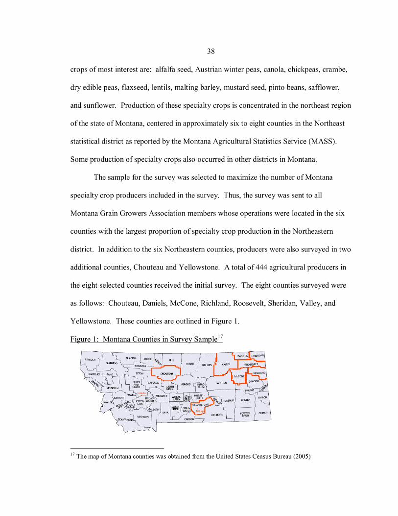
38

crops of most interest are: alfalfa seed, Austrian winter peas, canola, chickpeas, crambe,

dry edible peas, flaxseed, lentils, malting barley, mustard seed, pinto beans, safflower,

and sunflower. Production of these specialty crops is concentrated in the northeast region

of the state of Montana, centered in approximately six to eight counties in the Northeast

statistical district as reported by the Montana Agricultural Statistics Service (MASS).

Some production of specialty crops also occurred in other districts in Montana.

The sample for the survey was selected to maximize the number of Montana

specialty crop producers included in the survey. Thus, the survey was sent to all

Montana Grain Growers Association members whose operations were located in the six

counties with the largest proportion of specialty crop production in the Northeastern

district. In addition to the six Northeastern counties, producers were also surveyed in two

additional counties, Chouteau and Yellowstone. A total of 444 agricultural producers in

the eight selected counties received the initial survey. The eight counties surveyed were

as follows: Chouteau, Daniels, McCone, Richland, Roosevelt, Sheridan, Valley, and

Yellowstone. These counties are outlined in Figure 1.

Figure 1: Montana Counties in Survey Sample17

17 The map of Montana counties was obtained from the United States Census Bureau (2005)

39

Thus, the first stage of the survey process consisted of a non-random, purposive

sample whose respondents were chosen to increase the probability that individuals

receiving and responding to the surveys were specialty crop producers. The non-random

approach was adopted because, in the 2003 crop year, the acreage planted to specialty

crops in Montana accounted for only two and a half percent of total Montana cropland

acres. For any feasible sample size, a random sample was unlikely to result in a

sufficient number of observations for specialty crop production and marketing.

In addition to the producers surveyed from the Montana Grain Growers

Association sample, 26 additional American Indian producers in two of the eight counties

of interest, Roosevelt and Valley, were surveyed by authorized members of the Fort Peck

Community College. These respondents are members of the Fort Peck Indian

Reservation and provided a second opportunity to target agricultural producers in two of

the counties of interest in which specialty crops were produced.

The two-stage sampling approach was used for three reasons: to optimize the

accuracy of the information received, to obtain the highest response rate possible, and to

minimize respondent burden. The two-stage approach began with an initial one-page

survey accompanied by a letter from the Montana Grain Growers Association explaining

the purpose of the study18. The survey was mailed to all 444 members of the Montana

Grain Growers Association located in the eight target Montana counties with a self-

addressed stamped envelope for their return. The initial survey asked producers to

respond to three sets of questions. First, they were asked to fill in a table listing how 18 See Appendix B for a copy of both the authorized Montana Grain Growers Association letter and the Pre-Survey

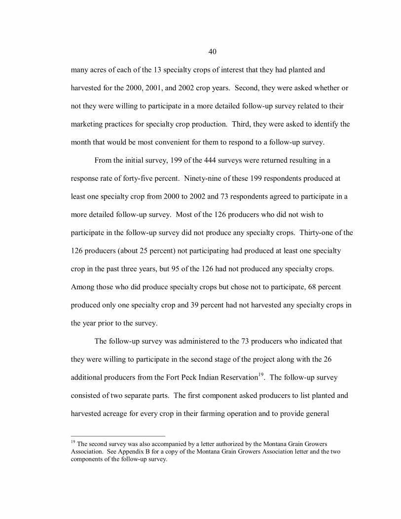
40

many acres of each of the 13 specialty crops of interest that they had planted and

harvested for the 2000, 2001, and 2002 crop years. Second, they were asked whether or

not they were willing to participate in a more detailed follow-up survey related to their

marketing practices for specialty crop production. Third, they were asked to identify the

month that would be most convenient for them to respond to a follow-up survey.

From the initial survey, 199 of the 444 surveys were returned resulting in a

response rate of forty-five percent. Ninety-nine of these 199 respondents produced at

least one specialty crop from 2000 to 2002 and 73 respondents agreed to participate in a

more detailed follow-up survey. Most of the 126 producers who did not wish to

participate in the follow-up survey did not produce any specialty crops. Thirty-one of the

126 producers (about 25 percent) not participating had produced at least one specialty

crop in the past three years, but 95 of the 126 had not produced any specialty crops.

Among those who did produce specialty crops but chose not to participate, 68 percent

produced only one specialty crop and 39 percent had not harvested any specialty crops in

the year prior to the survey.

The follow-up survey was administered to the 73 producers who indicated that

they were willing to participate in the second stage of the project along with the 26

additional producers from the Fort Peck Indian Reservation19. The follow-up survey

consisted of two separate parts. The first component asked producers to list planted and

harvested acreage for every crop in their farming operation and to provide general

19 The second survey was also accompanied by a letter authorized by the Montana Grain Growers Association. See Appendix B for a copy of the Montana Grain Growers Association letter and the two components of the follow-up survey.

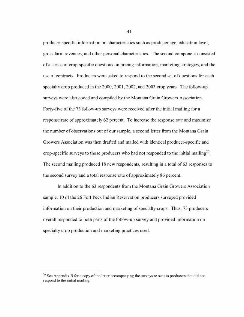
41

producer-specific information on characteristics such as producer age, education level,

gross farm revenues, and other personal characteristics. The second component consisted

of a series of crop-specific questions on pricing information, marketing strategies, and the

use of contracts. Producers were asked to respond to the second set of questions for each

specialty crop produced in the 2000, 2001, 2002, and 2003 crop years. The follow-up

surveys were also coded and compiled by the Montana Grain Growers Association.

Forty-five of the 73 follow-up surveys were received after the initial mailing for a

response rate of approximately 62 percent. To increase the response rate and maximize

the number of observations out of our sample, a second letter from the Montana Grain

Growers Association was then drafted and mailed with identical producer-specific and

crop-specific surveys to those producers who had not responded to the initial mailing20.

The second mailing produced 18 new respondents, resulting in a total of 63 responses to

the second survey and a total response rate of approximately 86 percent.

In addition to the 63 respondents from the Montana Grain Growers Association

sample, 10 of the 26 Fort Peck Indian Reservation producers surveyed provided

information on their production and marketing of specialty crops. Thus, 73 producers

overall responded to both parts of the follow-up survey and provided information on

specialty crop production and marketing practices used.

20 See Appendix B for a copy of the letter accompanying the surveys re-sent to producers that did not respond to the initial mailing.

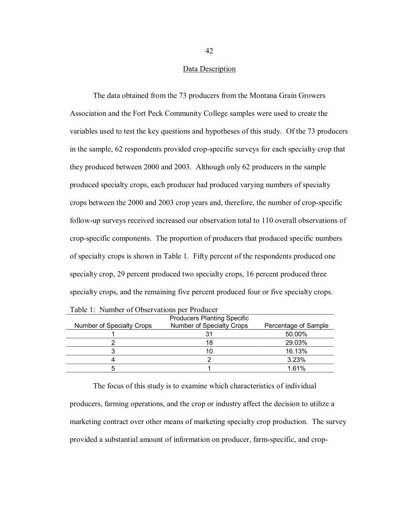
42

Data Description

The data obtained from the 73 producers from the Montana Grain Growers

Association and the Fort Peck Community College samples were used to create the

variables used to test the key questions and hypotheses of this study. Of the 73 producers

in the sample, 62 respondents provided crop-specific surveys for each specialty crop that

they produced between 2000 and 2003. Although only 62 producers in the sample

produced specialty crops, each producer had produced varying numbers of specialty

crops between the 2000 and 2003 crop years and, therefore, the number of crop-specific

follow-up surveys received increased our observation total to 110 overall observations of

crop-specific components. The proportion of producers that produced specific numbers

of specialty crops is shown in Table 1. Fifty percent of the respondents produced one

specialty crop, 29 percent produced two specialty crops, 16 percent produced three

specialty crops, and the remaining five percent produced four or five specialty crops.

Table 1: Number of Observations per Producer

Number of Specialty Crops Producers Planting Specific Number of Specialty Crops Percentage of Sample

1 31 50.00% 2 18 29.03% 3 10 16.13% 4 2 3.23% 5 1 1.61%

The focus of this study is to examine which characteristics of individual

producers, farming operations, and the crop or industry affect the decision to utilize a

marketing contract over other means of marketing specialty crop production. The survey

provided a substantial amount of information on producer, farm-specific, and crop-

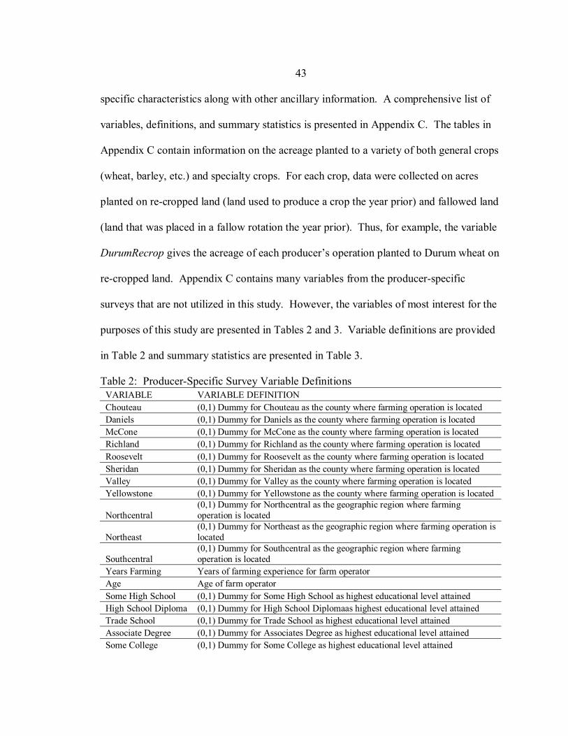
43

specific characteristics along with other ancillary information. A comprehensive list of

variables, definitions, and summary statistics is presented in Appendix C. The tables in

Appendix C contain information on the acreage planted to a variety of both general crops

(wheat, barley, etc.) and specialty crops. For each crop, data were collected on acres

planted on re-cropped land (land used to produce a crop the year prior) and fallowed land

(land that was placed in a fallow rotation the year prior). Thus, for example, the variable

DurumRecrop gives the acreage of each producer�s operation planted to Durum wheat on

re-cropped land. Appendix C contains many variables from the producer-specific

surveys that are not utilized in this study. However, the variables of most interest for the

purposes of this study are presented in Tables 2 and 3. Variable definitions are provided

in Table 2 and summary statistics are presented in Table 3.

Table 2: Producer-Specific Survey Variable Definitions VARIABLE VARIABLE DEFINITION Chouteau (0,1) Dummy for Chouteau as the county where farming operation is located Daniels (0,1) Dummy for Daniels as the county where farming operation is located McCone (0,1) Dummy for McCone as the county where farming operation is located Richland (0,1) Dummy for Richland as the county where farming operation is located Roosevelt (0,1) Dummy for Roosevelt as the county where farming operation is located Sheridan (0,1) Dummy for Sheridan as the county where farming operation is located Valley (0,1) Dummy for Valley as the county where farming operation is located Yellowstone (0,1) Dummy for Yellowstone as the county where farming operation is located

Northcentral (0,1) Dummy for Northcentral as the geographic region where farming operation is located

Northeast (0,1) Dummy for Northeast as the geographic region where farming operation is located

Southcentral (0,1) Dummy for Southcentral as the geographic region where farming operation is located

Years Farming Years of farming experience for farm operator Age Age of farm operator Some High School (0,1) Dummy for Some High School as highest educational level attained High School Diploma (0,1) Dummy for High School Diplomaas highest educational level attained Trade School (0,1) Dummy for Trade School as highest educational level attained Associate Degree (0,1) Dummy for Associates Degree as highest educational level attained Some College (0,1) Dummy for Some College as highest educational level attained

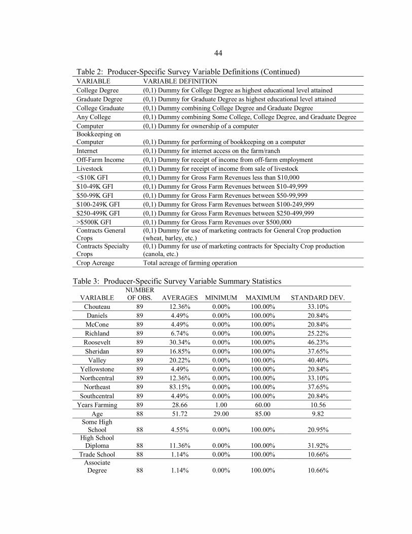
44

Table 2: Producer-Specific Survey Variable Definitions (Continued) VARIABLE VARIABLE DEFINITION College Degree (0,1) Dummy for College Degree as highest educational level attained Graduate Degree (0,1) Dummy for Graduate Degree as highest educational level attained College Graduate (0,1) Dummy combining College Degree and Graduate Degree Any College (0,1) Dummy combining Some College, College Degree, and Graduate Degree Computer (0,1) Dummy for ownership of a computer Bookkeeping on Computer (0,1) Dummy for performing of bookkeeping on a computer Internet (0,1) Dummy for internet access on the farm/ranch Off-Farm Income (0,1) Dummy for receipt of income from off-farm employment Livestock (0,1) Dummy for receipt of income from sale of livestock <$10K GFI (0,1) Dummy for Gross Farm Revenues less than $10,000 $10-49K GFI (0,1) Dummy for Gross Farm Revenues between $10-49,999 $50-99K GFI (0,1) Dummy for Gross Farm Revenues between $50-99,999 $100-249K GFI (0,1) Dummy for Gross Farm Revenues between $100-249,999 $250-499K GFI (0,1) Dummy for Gross Farm Revenues between $250-499,999 >$500K GFI (0,1) Dummy for Gross Farm Revenues over $500,000 Contracts General Crops

(0,1) Dummy for use of marketing contracts for General Crop production (wheat, barley, etc.)

Contracts Specialty Crops

(0,1) Dummy for use of marketing contracts for Specialty Crop production (canola, etc.)

Crop Acreage Total acreage of farming operation Table 3: Producer-Specific Survey Variable Summary Statistics

VARIABLE NUMBER OF OBS. AVERAGES MINIMUM MAXIMUM STANDARD DEV.

Chouteau 89 12.36% 0.00% 100.00% 33.10% Daniels 89 4.49% 0.00% 100.00% 20.84% McCone 89 4.49% 0.00% 100.00% 20.84% Richland 89 6.74% 0.00% 100.00% 25.22% Roosevelt 89 30.34% 0.00% 100.00% 46.23% Sheridan 89 16.85% 0.00% 100.00% 37.65% Valley 89 20.22% 0.00% 100.00% 40.40%

Yellowstone 89 4.49% 0.00% 100.00% 20.84% Northcentral 89 12.36% 0.00% 100.00% 33.10%

Northeast 89 83.15% 0.00% 100.00% 37.65% Southcentral 89 4.49% 0.00% 100.00% 20.84%

Years Farming 89 28.66 1.00 60.00 10.56 Age 88 51.72 29.00 85.00 9.82

Some High School 88 4.55% 0.00% 100.00% 20.95%

High School Diploma 88 11.36% 0.00% 100.00% 31.92%

Trade School 88 1.14% 0.00% 100.00% 10.66% Associate Degree 88 1.14% 0.00% 100.00% 10.66%

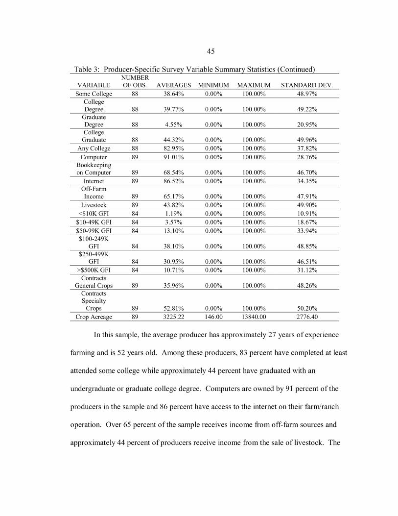
45

Table 3: Producer-Specific Survey Variable Summary Statistics (Continued)

VARIABLE NUMBER OF OBS. AVERAGES MINIMUM MAXIMUM STANDARD DEV.

Some College 88 38.64% 0.00% 100.00% 48.97% College Degree 88 39.77% 0.00% 100.00% 49.22%

Graduate Degree 88 4.55% 0.00% 100.00% 20.95% College

Graduate 88 44.32% 0.00% 100.00% 49.96% Any College 88 82.95% 0.00% 100.00% 37.82% Computer 89 91.01% 0.00% 100.00% 28.76%

Bookkeeping on Computer 89 68.54% 0.00% 100.00% 46.70%

Internet 89 86.52% 0.00% 100.00% 34.35% Off-Farm Income 89 65.17% 0.00% 100.00% 47.91%

Livestock 89 43.82% 0.00% 100.00% 49.90% <$10K GFI 84 1.19% 0.00% 100.00% 10.91%

$10-49K GFI 84 3.57% 0.00% 100.00% 18.67% $50-99K GFI 84 13.10% 0.00% 100.00% 33.94% $100-249K

GFI 84 38.10% 0.00% 100.00% 48.85% $250-499K

GFI 84 30.95% 0.00% 100.00% 46.51% >$500K GFI 84 10.71% 0.00% 100.00% 31.12%

Contracts General Crops 89 35.96% 0.00% 100.00% 48.26%

Contracts Specialty

Crops 89 52.81% 0.00% 100.00% 50.20% Crop Acreage 89 3225.22 146.00 13840.00 2776.40

In this sample, the average producer has approximately 27 years of experience

farming and is 52 years old. Among these producers, 83 percent have completed at least

attended some college while approximately 44 percent have graduated with an

undergraduate or graduate college degree. Computers are owned by 91 percent of the

producers in the sample and 86 percent have access to the internet on their farm/ranch

operation. Over 65 percent of the sample receives income from off-farm sources and

approximately 44 percent of producers receive income from the sale of livestock. The

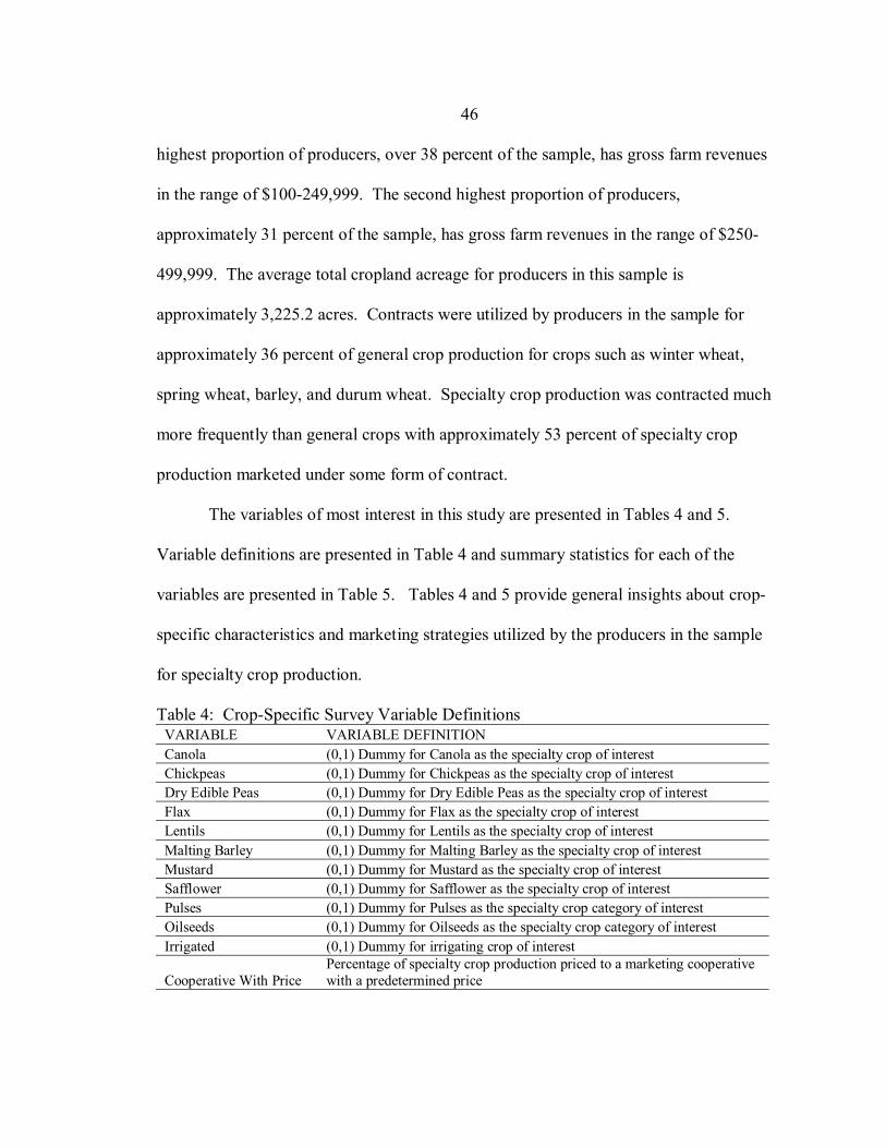
46

highest proportion of producers, over 38 percent of the sample, has gross farm revenues

in the range of $100-249,999. The second highest proportion of producers,

approximately 31 percent of the sample, has gross farm revenues in the range of $250-

499,999. The average total cropland acreage for producers in this sample is

approximately 3,225.2 acres. Contracts were utilized by producers in the sample for

approximately 36 percent of general crop production for crops such as winter wheat,

spring wheat, barley, and durum wheat. Specialty crop production was contracted much

more frequently than general crops with approximately 53 percent of specialty crop

production marketed under some form of contract.

The variables of most interest in this study are presented in Tables 4 and 5.

Variable definitions are presented in Table 4 and summary statistics for each of the

variables are presented in Table 5. Tables 4 and 5 provide general insights about crop-

specific characteristics and marketing strategies utilized by the producers in the sample

for specialty crop production.

Table 4: Crop-Specific Survey Variable Definitions VARIABLE VARIABLE DEFINITION Canola (0,1) Dummy for Canola as the specialty crop of interest Chickpeas (0,1) Dummy for Chickpeas as the specialty crop of interest Dry Edible Peas (0,1) Dummy for Dry Edible Peas as the specialty crop of interest Flax (0,1) Dummy for Flax as the specialty crop of interest Lentils (0,1) Dummy for Lentils as the specialty crop of interest Malting Barley (0,1) Dummy for Malting Barley as the specialty crop of interest Mustard (0,1) Dummy for Mustard as the specialty crop of interest Safflower (0,1) Dummy for Safflower as the specialty crop of interest Pulses (0,1) Dummy for Pulses as the specialty crop category of interest Oilseeds (0,1) Dummy for Oilseeds as the specialty crop category of interest Irrigated (0,1) Dummy for irrigating crop of interest

Cooperative With Price Percentage of specialty crop production priced to a marketing cooperative with a predetermined price

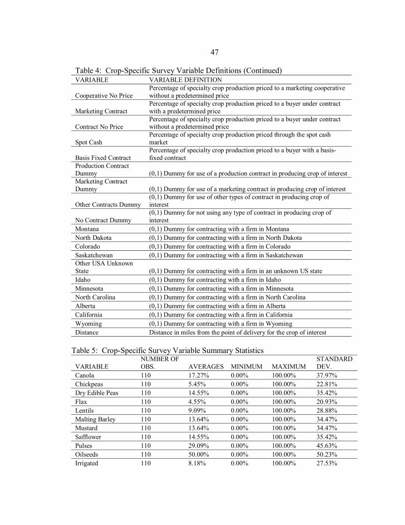
47

Table 4: Crop-Specific Survey Variable Definitions (Continued) VARIABLE VARIABLE DEFINITION

Cooperative No Price Percentage of specialty crop production priced to a marketing cooperative without a predetermined price

Marketing Contract Percentage of specialty crop production priced to a buyer under contract with a predetermined price

Contract No Price Percentage of specialty crop production priced to a buyer under contract without a predetermined price

Spot Cash Percentage of specialty crop production priced through the spot cash market

Basis Fixed Contract Percentage of specialty crop production priced to a buyer with a basis-fixed contract

Production Contract Dummy (0,1) Dummy for use of a production contract in producing crop of interest Marketing Contract Dummy (0,1) Dummy for use of a marketing contract in producing crop of interest

Other Contracts Dummy (0,1) Dummy for use of other types of contract in producing crop of interest

No Contract Dummy (0,1) Dummy for not using any type of contract in producing crop of interest

Montana (0,1) Dummy for contracting with a firm in Montana North Dakota (0,1) Dummy for contracting with a firm in North Dakota Colorado (0,1) Dummy for contracting with a firm in Colorado Saskatchewan (0,1) Dummy for contracting with a firm in Saskatchewan Other USA Unknown State (0,1) Dummy for contracting with a firm in an unknown US state Idaho (0,1) Dummy for contracting with a firm in Idaho Minnesota (0,1) Dummy for contracting with a firm in Minnesota North Carolina (0,1) Dummy for contracting with a firm in North Carolina Alberta (0,1) Dummy for contracting with a firm in Alberta California (0,1) Dummy for contracting with a firm in California Wyoming (0,1) Dummy for contracting with a firm in Wyoming Distance Distance in miles from the point of delivery for the crop of interest

Table 5: Crop-Specific Survey Variable Summary Statistics

VARIABLE NUMBER OF OBS. AVERAGES MINIMUM MAXIMUM

STANDARD DEV.

Canola 110 17.27% 0.00% 100.00% 37.97% Chickpeas 110 5.45% 0.00% 100.00% 22.81% Dry Edible Peas 110 14.55% 0.00% 100.00% 35.42% Flax 110 4.55% 0.00% 100.00% 20.93% Lentils 110 9.09% 0.00% 100.00% 28.88% Malting Barley 110 13.64% 0.00% 100.00% 34.47% Mustard 110 13.64% 0.00% 100.00% 34.47% Safflower 110 14.55% 0.00% 100.00% 35.42% Pulses 110 29.09% 0.00% 100.00% 45.63% Oilseeds 110 50.00% 0.00% 100.00% 50.23% Irrigated 110 8.18% 0.00% 100.00% 27.53%

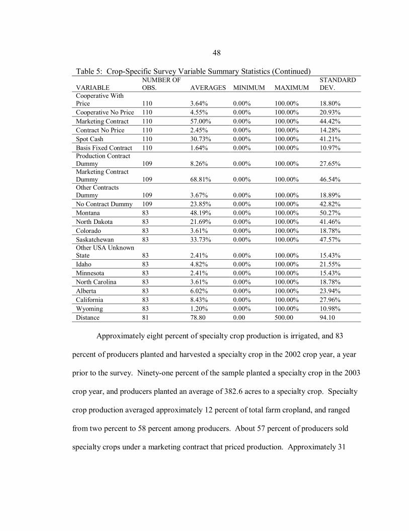
48

Table 5: Crop-Specific Survey Variable Summary Statistics (Continued)

VARIABLE NUMBER OF OBS. AVERAGES MINIMUM MAXIMUM

STANDARD DEV.

Cooperative With Price 110 3.64% 0.00% 100.00% 18.80% Cooperative No Price 110 4.55% 0.00% 100.00% 20.93% Marketing Contract 110 57.00% 0.00% 100.00% 44.42% Contract No Price 110 2.45% 0.00% 100.00% 14.28% Spot Cash 110 30.73% 0.00% 100.00% 41.21% Basis Fixed Contract 110 1.64% 0.00% 100.00% 10.97% Production Contract Dummy 109 8.26% 0.00% 100.00% 27.65% Marketing Contract Dummy 109 68.81% 0.00% 100.00% 46.54% Other Contracts Dummy 109 3.67% 0.00% 100.00% 18.89% No Contract Dummy 109 23.85% 0.00% 100.00% 42.82% Montana 83 48.19% 0.00% 100.00% 50.27% North Dakota 83 21.69% 0.00% 100.00% 41.46% Colorado 83 3.61% 0.00% 100.00% 18.78% Saskatchewan 83 33.73% 0.00% 100.00% 47.57% Other USA Unknown State 83 2.41% 0.00% 100.00% 15.43% Idaho 83 4.82% 0.00% 100.00% 21.55% Minnesota 83 2.41% 0.00% 100.00% 15.43% North Carolina 83 3.61% 0.00% 100.00% 18.78% Alberta 83 6.02% 0.00% 100.00% 23.94% California 83 8.43% 0.00% 100.00% 27.96% Wyoming 83 1.20% 0.00% 100.00% 10.98% Distance 81 78.80 0.00 500.00 94.10

Approximately eight percent of specialty crop production is irrigated, and 83

percent of producers planted and harvested a specialty crop in the 2002 crop year, a year

prior to the survey. Ninety-one percent of the sample planted a specialty crop in the 2003

crop year, and producers planted an average of 382.6 acres to a specialty crop. Specialty

crop production averaged approximately 12 percent of total farm cropland, and ranged

from two percent to 58 percent among producers. About 57 percent of producers sold

specialty crops under a marketing contract that priced production. Approximately 31

49

percent of specialty crops produced were sold in the spot cash market. The average

distance to a delivery point for specialty crops was approximately 79 miles.

Specialty crop acreage accounted for approximately 14 percent of total cropland

acres in the sample. Overall specialty crop acres in the state of Montana for the 2003

crop year accounted for two and a half percent of total cropland acres. Approximately 71

percent of the entire specialty crop acreage produced in the sample was sold under some

form of contract, while 29 percent was not sold under contract.

Contracting also varied across individual crops. Among crops grown by at least

five producers, safflower was the most frequently contracted crop with over 97 percent of

safflower acreage contracted. Approximately 81 percent of malting barley acres were

contracted, 76 percent of dry edible pea acreage was contracted, 73 percent of mustard

seed production was contracted, and approximately 72 percent of lentil acreage was

contracted. The three crops with the lowest percentage of total sample acreage contracted

were chickpeas (57 percent), canola (47 percent), and flaxseed (12 percent).

Individual producers within crops also utilized contracts at various rates as well.

For malting barley and mustard seed, 15 respondents produced both crops and 14 of the

15 utilized contracts in the production of both crops. Safflower was contracted by 12 of

13 respondents, and lentils were contracted by 7 of 8 respondents. Canola was contracted

by 12 of 19 respondents, chickpeas by three of five respondents, dry edible peas by five

of 10 respondents, and flaxseed was contracted by two of five respondents.

50

Summary

The use of contracts varies among all producers and all crops, but it is also

apparent that the use of contracts for marketing specialty crop production varies

substantially across individual crops and among producers of each specific specialty crop.

The data described in this chapter will be used to test the key hypotheses of this study

about the determinants of marketing contract use by specialty crop producers. The data

obtained from both of the follow-up surveys of Montana Grain Growers Association

members provides information to investigate the effects of specific personal, farm-

specific, and crop-specific characteristics on the adoption of marketing contracts and the

proportion of production contracted decision. The next chapter will outline the empirical

models utilized to test the hypotheses with the data outlined in this chapter and present

results of those tests and hypotheses.

51

CHAPTER 6

EMPIRICAL MODELS AND RESULTS

The purpose of this study is to examine empirically the characteristics that affect

the adoption of marketing contracts and the proportion of production contracted by

specialty crop producers. This chapter describes the estimation procedures used to obtain

parameter estimates for models of adoption and the proportion of production contracted

by specialty crop producers. In addition, this chapter presents the results of the empirical

analysis.

Empirical Estimation Setup

In Chapter 3, several hypotheses were developed about how specific

characteristics influence a producer�s specialty crop marketing decisions. Personal, farm-

specific, and crop-specific characteristics comprise the three general categories of

variables that influence a producer�s decision about whether to adopt marketing contracts

and their decision about what proportion of output to sell under these contracts.

A producer�s decision about whether or not to adopt a marketing contract is

represented by ci, where ci = 0 represents a decision not to adopt marketing contracts and

ci = 1 represents a decision to adopt marketing contracts. The adoption decision is

formally related to a matrix of observable personal, farm, and crop characteristics, zi,

through the function,

(5.1) P(ci = 1) = h(γ′zi, εci)

52

In equation (5.1), P(ci = 1) is the probability that marketing contracts will be adopted, γ is

a parameter vector and εci is the error term representing unmeasured factors relating to

adoption of marketing contracts.

Probability models such as equation (5.1) are typically estimated empirically

using either logit or probit models. Both are binary probability models in which the

dependent variable is distributed between 0 and 1. The functional form of h in equation

(5.1) is determined by the assumptions placed upon the distribution of the error term, εci

(Liao 1994; Greene 2000). Two alternative assumptions are made about the distribution

of error terms in binary probability models. The first is that the error term follows a

logistic distribution, which yields a logit model. The second is that the error term follows

a normal distribution, which yields a probit model. Liao (1994) notes that these

assumptions will often yield similar parameter estimates. Greene (2000) also states that it

is difficult to justify the choice of one distribution over the other on theoretical grounds.

The logit distribution is fatter in the tails and therefore may be more appropriate with an

extremely large number of observations. Previous studies of the marketing contract

adoption decision have utilized the normality assumption for the error term distribution.

In addition, the number of observations available for analysis in this study is relatively

small. Thus, probit models are used to estimate equation (5.1).

Conditional upon the decision to adopt marketing contracts, the ith producer must

determine the proportion of specialty crop production to be contracted, αi, where αi > 021.

21 A producer can contract more than their actual post-harvest production, and therefore αi is not constrained from above. See Katchova and Miranda (2004) for a more detailed explanation of the proportion of production to be contracted decision and the bounds of αi.

53

This decision is also a function of a set of personal, farm-specific, and crop-specific

characteristics, xi, which may be the same or a different set of variables than the set that

influence the adoption decision, zi; that is, xi and zi may or may not be the same matrix of

variables. Formally, the decision about what proportion of production to contract can be

represented as follows:

(5.2) αi = gα(βα′xi, εαi)

In equation (5.2), βα is a parameter vector and the error term, εαi, represents unmeasured

factors relating to the decision of what proportion to contract. Equation (5.2) is often

estimated empirically using a Tobit model in which the data is assumed to be censored.

Censored observations imply that there are known values of the explanatory variables,

but the corresponding values of the dependent variable are unobservable. A second

empirical method is to utilize a truncated regression that truncates the sample, implying

that values of the explanatory variables are known only when the dependent variable is

observed. Either a Tobit regression model or a truncated regression could be utilized to

estimate equation (5.2).

Kennedy (2003) notes that one drawback to using a Tobit model is the assumption

that the equation determining whether or not an observation is included in the sample is

the same as the equation that yields the value of the dependent variable. In the context of

the maximization problem for specialty crop producers, a Tobit model would imply that

the same set of characteristics affects both the adoption and the proportion of production

contracted decisions in the same way, yielding a one-step maximization process. Lin and

Schmidt (1984) discuss the restrictive nature of the assumptions of a Tobit model in their

54

example of a Tobit model for the loss due to fire in buildings. They argue that older

buildings are more likely to have fires, but because newer buildings are more valuable,

fires in older buildings would result in smaller financial losses than would fires in newer

buildings. Therefore, the coefficient on �Age� would have a different sign in a probit or

logit model explaining whether or not a building would experience a fire than in a

truncated regression explaining the size of the subsequent financial loss. Accounting for

these differences is impossible in a Tobit model because of the restriction it places on the

coefficients that affect both the probability of a fire and the size of the loss.

In the context of this study, a Tobit model would imply that in equations (5.1) and

(5.2), the characteristics which influence the decision to adopt contracts, zi, would be

identical to those characteristics which influence the decision of what proportion of

production to contract, xi. In addition, the characteristics would also influence each

decision in the same way, implying that the estimated parameter vectors would also be

identical. A characteristic that significantly increases the probability of marketing

contract adoption would also significantly increase the proportion of production which

the producer would contract.

Cragg (1971) relaxed the assumption that the same variables and the same vector

of parameters affect both decisions in a Tobit model. Katchova and Miranda (2004)

applied Cragg�s approach to a producer�s marketing decision by estimating a double-

hurdle model in which, initially, a producer decides whether to adopt marketing

contracts, estimated through an independent probit model. Once the �hurdle� is crossed

and the producer has adopted marketing contracts (that is, ci = 1), then a truncated

55

regression of the proportion of production to be contracted is estimated. The double-

hurdle model serves as an alternative to the Tobit model22.

In order to test the more restrictive Tobit model against the more general two-step

model, Cragg proposed a likelihood ratio statistic to test for which approach is more

appropriate (Greene 2000). The null hypothesis is that the Tobit model is the appropriate

modeling technique and the alternative hypothesis is that Cragg�s model (a separate

probit and truncated regression) is the appropriate model. The test statistic is computed

by fitting a Tobit model using a given set of explanatory variables and then separately

fitting a probit model and a truncated model using the same set of explanatory variables.

Utilizing the logs of the likelihood values for the three models, Cragg�s double-hurdle

likelihood ratio statistic, λ, is as follows:

(5.3) [ ]T P TR = -2 log L - (log L + log L )λ

In equation (5.3), LT is the likelihood value for the Tobit model, LP is the likelihood value

for the probit model, and LTR is the likelihood value for the truncated regression model.

The likelihood ratio test statistic, λ, is distributed as chi-square (χ2) with R degrees of

freedom, where R is the number of independent variables including a constant. Cragg�s

test statistic (equation (5.3)) is estimated for several alternative modeling specifications

of the contracting decisions. As discussed further below, in all cases, the estimated

values of the test statistic, λ, are significantly larger than the critical χ2 values at the

22 Katchova and Miranda (2004) note that the truncation problem considered here is different from a �sample selection� problem which is commonly estimated by Heckman�s two-step procedure. Heckman�s model is not appropriate for problems like these because the quantity contracted for farmers who have not adopted marketing contracts are observed as being equal to zero rather than being literally unobserved. Please see Katchova and Miranda (2004), Greene (2000), and Lin and Schmidt (1984) for a more thorough discussion of this sampling problem.

56

ninety-nine percent confidence level. Thus, this study estimates Cragg�s double-hurdle

models to explain the contracting adoption and contract use decisions.

Heteroscedasticity is often present in cross-section data of the type used in this

study. The sample of survey respondents is drawn from a tight geographic distribution

and multiple observations come from single producers as each producer may produce

more than one specialty crop. Therefore, there are systematic relationships among the

error terms associated with individual observations. Greene (2000) notes that maximum

likelihood estimators are not consistent in the presence of any form of heteroscedasticity,

unmeasured heterogeneity, omitted variables which are orthogonal to the included

variables, nonlinearity of the functional form of the index, or errors in distributional

assumptions. In the case of heteroscedasticity, the concern here, Greene recommends

using White�s robust �sandwich� estimator for the asymptotic covariance matrix in order

to control for heteroscedasticity. Thus, all of the standard errors in every reported model

are computed using the Huber/White sandwich estimator of variances within Stata to

account for the potential presence of heteroscedasticity in the error structure.

Empirical Variable Definitions and Expectations

The empirical models used to examine the adoption decision in equation (5.1) are

probit models and the empirical models used to estimate the proportion of production to

contract decision in equation (5.2) are truncated regression models. The variables

incorporated in the matrix zi for the adoption decision and the matrix xi for the proportion

of production to contract decision are personal, farm-specific, and crop-specific

57

characteristics that affect both marketing decisions independently for individual specialty

crop producers.

Variables for Personal Characteristics

The personal characteristic variables in matrices zi and xi are as follows. The

producer�s age, Age, is measured in years and serves as a proxy for experience.

Experience may have a positive or negative effect on both the marketing contract

adoption decision and the proportion of production to contract decision. As discussed in

Chapter 3, farmers may become more or less risk-averse as experience increases, and

therefore the effects of experience on both the adoption of a marketing contract as a risk-

reducing mechanism and the proportion of production contracted is uncertain. Thus, the

expected effect of Age is uncertain.

A producer�s level of education, as measured through the dummy variables Some

College, College Degree, and Any College, serves as a proxy for human capital. Some

College controls for those producers who attended college but did not graduate, College

Degree controls for those who graduated college with an undergraduate or graduate

degree, and Any College controls for both those producers who attended college, whether

or not they graduated. The effects of human capital on marketing decisions are unclear.

Producers with a higher level of education have lower costs of understanding and

interpreting the terms of marketing contracts (Musser et al. 1996), increasing the

likelihood of adoption as well as the proportion of production contracted. However,

producers with higher levels of education and human capital may be less risk-averse and,

58

therefore, less likely to use marketing contracts as a risk reducing mechanism (Shapiro

and Brorsen 1988).

Willingness to adopt new technology is proxied by the dummy variables Internet

and Bookkeeping on Computer, which measure a producer�s use of the internet in

managing the farm operation and computer-based programs to manage bookkeeping.

Producers who use the internet and bookkeeping programs on the computer are assumed

to be more likely to adopt marketing contracts and to market a larger proportion of their

production with marketing contracts (Goodwin and Schroeder 1994).

Variables for Farm-Specific Characteristics

Geographic-specific information such as the number of specialty crop buyers in a

county or region, climate, and soil type varies by county and region, but data on these

variables were not available. A priori, the effects of each county or regional dummy

variable on a farm�s marketing decisions are difficult to predict, but these effects should

still be taken into account. Geographic effects upon marketing decisions were initially

proxied by eight county dummy variables: Chouteau, Daniels, McCone, Richland,

Roosevelt, Sheridan, Valley, and Yellowstone. These variables were intended to capture

county-specific effects. However, multicollinearity appeared to be a problem within the

set of county dummy variables. Thus, regional dummy variables are utilized. Northeast

consists Daniels, McCone, Richland, Roosevelt, Sheridan, and Valley, Northcentral

59

consists of Chouteau, and Southcentral consists of Yellowstone23. The county and

regional dummy variables also proxy unknown, random conditions and characteristics of

the producer�s geographic location which are assumed to be factored into a producer�s

expectation of crop yield. The contracted proportion of production depends upon these

unknown, random characteristics that directly affect crop yield, and therefore the

geographic variables help account for yield-affecting random characteristics.

The total area of a farming operation, Crop Acreage, serves as proxy for the size

of the entire farming operation. Crop-specific revenues would also control for the size

and scope for the production of a specific crop, but yield and price data were unavailable

for the purposes of this study. Therefore, Crop Acreage serves as the main proxy for

farm size and the size and scope of the production of individual crops. Farm size is

expected to have a positive effect on both contracting decisions as producers operating

large farms may have economies of size with respect to their ability to spread costs

incurred in learning about and entering into contracts over a large number of acres

(Shapiro and Brorsen 1988; Sartwelle et al. 2000). A priori, the contract adoption and

proportion of production contracted decisions are both expected to be positively related to

Crop Acreage.

Total gross farm income (GFI) is an indicator of both farm size and farm wealth.

Data were available only on the range of GFI within which each farm�s income falls.

The ranges of GFI included $0-99,000, $100-249,000, $250-499,000, and $500,000 and

23 The regional dummy variables , Northeast, Northcentral, and Southcentral were constructed following the regional classification from the Montana Agricultural Statistics Service by which each of the individual county variables was classified into one of the three regional dummy variables.

60

greater. Three dummy variables, $100-249K GFI, $250-499K GFI, and >$500K GFI are

utilized to account for the various levels of GFI, assuming that the base dummy variable

is $0-99K GFI. Economies of size from higher levels of GFI would imply a predicted

positive effect on both marketing decisions (Asplund et al. 1989; Edelman et al. 1990;

Katchova and Miranda 2004). However, a potential wealth effect is associated with

higher levels of gross income. Thus, from the wealth effect, producers may become less

risk-averse24 and thus both marketing contract decisions may be negatively related to

increasing gross farm income (Musser et al. 1996). Therefore, a priori the effects on

contracting decisions of each gross farm income variable are uncertain.

Sources of additional non-crop farm income are measured through the dummy

variables Off-Farm Income and Livestock, which take on a value of one if the farm

receives off-farm income or income from the sale of livestock. These variables proxy for

enterprise diversification, as farms with multiple sources of income are considered to be

diversified. For a diversified farm, the income from the sale of general and specialty

crops is not as vital as it is to a farm whose sole source of income is crop-related income

as diversified farms have alternative sources of risk management available. Therefore,

contract adoption and the proportion of production contracted are likely to be inversely

related to both Off-Farm Income and Livestock.

24 Although increasing wealth is hypothesized to decrease the level of absolute risk-aversion, the effect of increasing wealth on relative risk-aversion is uncertain. Therefore, when hypothesizing the effects of wealth on the proportion of production contracted decision, the effect is typically more related to relative risk-aversion. However, in this study, controlling for total crop acreage allows the wealth effect to be analyzed from an absolute risk-aversion perspective for both the adoption and the contracted proportion of production decisions.

61

Variables for Crop-Specific Characteristics Marketing channels differ among crops. For some crops, the spot cash market is

well-established and locally available, but for others the spot cash market is thin and

available only in few locations. For example, some crops that can be utilized for multiple

end-products have several markets in which the production can be delivered. In addition,

crop-specific characteristics also influence a producer�s expectations about crop yield and

crop yield variability, which affects the proportion of production contracted by individual

producers. Therefore, crop-specific variables may serve as instrument variables for

unknown and random characteristics of individual crops and the response of individual

crops to random factors, all of which influence crop yields. Crop-specific effects upon

marketing decisions were initially proxied by eight crop dummy variables Canola,

Chickpeas, Dry Edible Peas, Flax, Lentils, Malting Barley, Mustard, and Safflower.

These variables were intended to capture crop-specific effects. However,

multicollinearity appeared to be a problem within this set of crop dummy variables.

Thus, instead, two dummy variables for categories of crops. Oilseeds consist of Canola,

Flax, Mustard, and Safflower, Pulses consist of Chickpeas, Dry Edible Peas, and Lentils,

and Malting Barley is its own category due to its unique crop-specific qualities and lack

of substitutes. Although some crops in the Pulses category may be used as livestock feed

and are therefore less likely to be contracted, not all pulse crops are appropriate for use as

feed for livestock. There are unknown characteristics accounted for in crop-specific

variables and the categorical dummy variables. Thus, it is not possible to make distinct

predictions about the relation of specific crop categorical variables to either contracting

62

decision. Given that Pulses serve as the base dummy variable category, a priori it is not

clear how both of the contracting decisions are related to the Oilseeds and Malting Barley

variables.

Distance to market for the delivery of a specialty crop, Distance, is measured in

miles and serves as a proxy for the transportation costs incurred in delivering contracted

production to the market. Data on the difference between the distance to the contractor

and the spot cash market were not available. Thus, the proxy variable Distance is not an

ideal explanatory variable and, a priori, its effect on marketing decisions is uncertain.

One indicator of production costs, yield variability, and crop quality of a specific

crop is whether or not the crop is irrigated. Thus, the dummy variable Irrigated is

included in the model. As production costs increase, ceteris paribus, a producer may be

more likely to ensure a guaranteed price for the crop. Irrigated crops are expected to

have higher production costs per acre, and therefore marketing contract adoption is

expected to be positively related to the variable Irrigated. In addition, yields for

irrigated crops are typically less variable than dryland crops. Thus, the likelihood that a

producer will have to default on delivery of production to the contractor is lower. Buyers

of specialty crop production may also want to secure a higher proportion of irrigated crop

production because of the predictable and more consistent production from irrigated

crops. Therefore, a producer may be willing to contract a larger proportion of output, and

the proportion contracted decision is thus expected to be positively related to the variable

Irrigated.

63

Empirical Estimation Models and Estimation Methods

Several alternative empirical models are estimated to investigate how personal,

farm-specific, and crop-specific characteristics independently influence both the decision

to use marketing contracts and the proportion of production to be contracted. Model

parameter estimates for the marketing contract adoption decision and the contracted

proportion of production decision are presented in Tables 6 and 7 respectively. Table 8

presents Cragg�s double-hurdle likelihood ratio test statistics and the results of likelihood

ratio tests for joint significance of subsets of various variables. The contract adoption

models are estimated as probit models in Stata in which the dependent variable is

Marketing Contract, a zero-one dummy variable for the adoption of marketing

contracts25. The contracted proportion of production models are estimated as truncated

regressions in Stata in which the dependent variable is Contracted Proportion, a

continuous variable measuring the proportion of production marketed under contract to

buyers26. To correct for the potential problem of heteroscedasticity, all of the models

were estimated in Stata using the robust standard error procedure.

The initial models, Adoption Model (1) and Proportion Contracted Model (1),

incorporate all of the personal, farm-specific, and crop-specific characteristics described

25 Each adoption model is estimated using the �dprobit� option which, rather than reporting coefficients, reports the change in the probability for an infinitesimal change in each independent continuous variable. Also, �dprobit� by default yields the discrete change in the probability for dummy variables. Therefore, instead of coefficients, �Df/Dx� is reported in table 5.1. 26 The truncated regressions estimated in Stata truncate the sample to include observations whose response for �Proportion of Production Contracted� is greater than zero. Of the 109 observations in the sample, 35 observations were truncated at zero because their proportion of production contracted was equal to zero.

64

above, including county-specific and crop-specific dummy variables. They are defined

as follows:

Adoption Model (1): P(ci = 1) = φ(γ0 + γ1Agei + γ2Some Collegei + γ3College Degreei + γ4Interneti +

γ5Bookkeeping on Computeri + γ6Chouteaui + γ7Danielsi + γ8McConei + γ9Richlandi + γ10Roosevelti + γ11Valleyi + γ12Crop Acreagei + γ13$100-249K GFIi + γ14$250-499K GFIi + γ15>$500K GFIi + γ16Off-Farm Incomei + γ17Livestocki + γ18Canolai + γ19Chickpeasi + γ20Dry Edible Peasi + γ20Flaxi + γ21Lentilsi + γ22Malting Barleyi + γ23Mustardi + γ24Saffloweri + γ25Distancei + γ26Irrigatedi + εci)

Proportion Contracted Model (1): αi|ci=1 = β0 + β1Agei + β2Some Collegei + β3College Degreei + β4Interneti +

β5Bookkeeping on Computeri + β6Chouteaui + β7Danielsi + β8McConei + β9Richlandi + β10Roosevelti + β11Valleyi + β12Crop Acreagei + β13$100-249K GFIi + β14$250-499K GFIi + β15>$500K GFIi + β16Off-Farm Incomei + β17Livestocki + β18Canolai + β19Chickpeasi + β20Dry Edible Peasi + β20Flaxi + β21Lentilsi + β22Malting Barleyi + β23Mustardi + β24Saffloweri + β25Distancei + β26Irrigatedi + εαi

Parameter estimates for these initial models are presented in Tables 6 and 7. Inspection

of the variance/covariance correlation matrix indicated that, as noted above, individual

crop and county variables were highly correlated27. For each model, a likelihood ratio

test was performed on the joint significance of both individual crop variables and

individual county variables, and the test statistics are presented in Table 8. The

individual crop variables were jointly significant in both of the models, and the individual

county variables were significant in the Adoption Model, but not in the Proportion

Contracted Model. Therefore, categorical variables for crop type replaced individual

27 Appendix D presents results of variance/covariance correlation matrices for each empirical model. In addition, because the sample only consisted of 109 observations, the power of the model decreases with inclusion of additional variables.

65

crop dummy variables in each initial model, and individual county variables were

replaced by regional dummy variables in the adoption model. In addition, Some College

was highly correlated with College Degree and therefore Some College was also omitted.

Substituting categorical variables for individual crop dummy variables in each

initial model and categorical geographic variables for individual county variables in

Adoption Decision (1), and removing Some College to obtain the effects of controlling

for a college degree results in a second set of estimated models, defined as:

Adoption Model (2): P(ci = 1) = φ(γ0 + γ1Agei + γ2College Degreei + γ3Interneti + γ4Bookkeeping on

Computeri + γ5Northcentrali + γ6Southcentrali + γ7Crop Acreagei + γ8$100-249K GFIi + γ9$250-499K GFIi + γ10>$500K GFIi + γ11Off-Farm Incomei + γ12Livestocki + γ13Oilseedi + γ14Malting Barleyi + γ15Distancei + γ16Irrigatedi + εci)

Proportion Contracted Model (2): αi|ci=1 = β0 + β1Agei + β2College Degreei + β3Interneti + β4Bookkeeping on

Computeri + β5Crop Acreagei + β6$100-249K GFIi + β7$250-499K GFIi + β8>$500K GFIi + β9Off-Farm Incomei + β10Livestocki + β11Oilseedi + β12Malting Barleyi + β13Distancei + β14Irrigatedi + εαi

Parameter estimates for Adoption Model (2) and Proportion Contracted Model (2)

are presented in Tables 6 and 7 respectively. Inspection of the variance/covariance

correlation matrix for both models indicates that there was no significant

multicollinearity among the explanatory variables in Adoption Model (2). However,

some degree of collinearity appeared to exist between Crop Acreage, the Gross Farm

Income (GFI) variables, and Livestock and Off-Farm Income in Proportion Contracted

Model (2). Thus, Crop Acreage was omitted from subsequent proportion contracted

66

models. In addition, in both of the above models the effects of human capital

accumulation are accounted for by the variable College Degree. To estimate human

capital accumulation for those with no college education at all against those that attended

or graduate from college, the variable Any College was substituted for College Degree.

Thus, a third set of models is estimated in which the base educational category is changed

to those not having attended any college in both the adoption and contracted proportion

of production decisions, and Crop Acreage was omitted from Proportion Contracted

Model (2). The third set of models is therefore:

Adoption Model (3): P(ci = 1) = φ(γ0 + γ1Agei + γ2Any Collegei + γ3Interneti + γ4Bookkeeping on

Computeri + γ5Northcentrali + γ6Southcentrali + γ7Crop Acreagei + γ8$100-249K GFIi + γ9$250-499K GFIi + γ10>$500K GFIi + γ11Off-Farm Incomei + γ12Livestocki + γ13Oilseedi + γ14Malting Barleyi + γ15Distancei + γ16Irrigatedi + εci)

Proportion Contracted Model (3): αi|ci=1 = β0 + β1Agei + β2Any Collegei + β3Interneti + β4Bookkeeping on Computeri

+ β5$100-249K GFIi + β6$250-499K GFIi + β7>$500K GFIi + β8Off-Farm Incomei + β9Livestocki + β10Oilseedi + β11Malting Barleyi + β12Distancei + β13Irrigatedi + εαi

Parameter estimates from Adoption Model (3) and Proportion Contracted Model (3) are

also reported in Tables 6 and 7. Inspection of the variance/covariance correlation matrix

for these models did not indicate the presence of multicollinearity. Thus, the focus of the

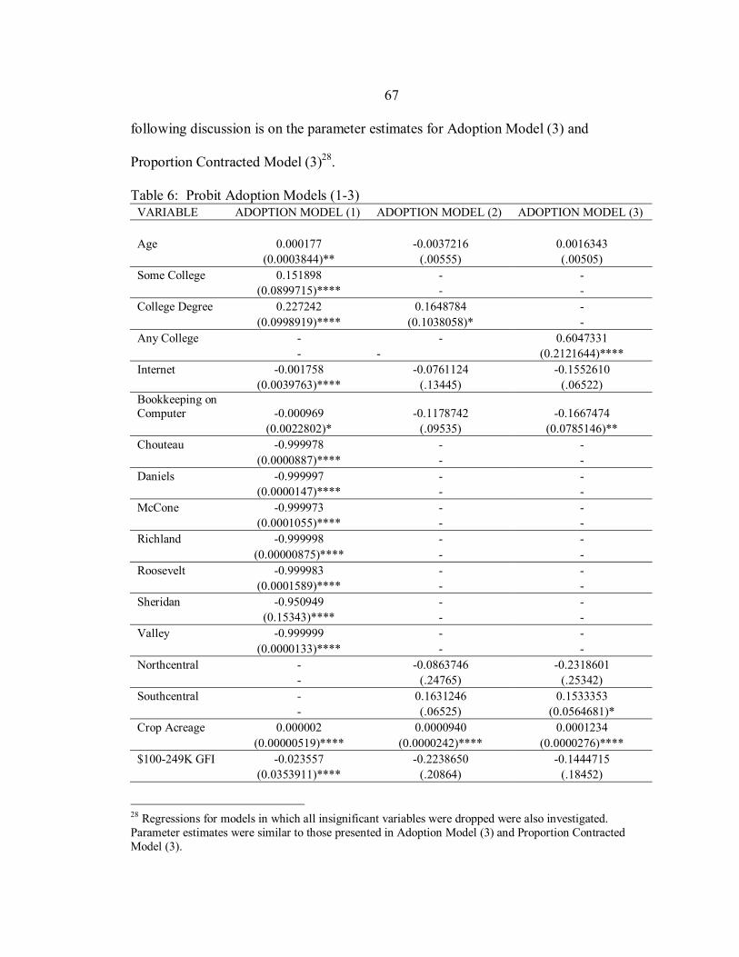
67

following discussion is on the parameter estimates for Adoption Model (3) and

Proportion Contracted Model (3)28.

Table 6: Probit Adoption Models (1-3) VARIABLE ADOPTION MODEL (1) ADOPTION MODEL (2) ADOPTION MODEL (3) Age 0.000177 -0.0037216 0.0016343 (0.0003844)** (.00555) (.00505) Some College 0.151898 - - (0.0899715)**** - - College Degree 0.227242 0.1648784 - (0.0998919)**** (0.1038058)* - Any College - - 0.6047331 - - (0.2121644)**** Internet -0.001758 -0.0761124 -0.1552610 (0.0039763)**** (.13445) (.06522) Bookkeeping on Computer -0.000969 -0.1178742 -0.1667474 (0.0022802)* (.09535) (0.0785146)** Chouteau -0.999978 - - (0.0000887)**** - - Daniels -0.999997 - - (0.0000147)**** - - McCone -0.999973 - - (0.0001055)**** - - Richland -0.999998 - - (0.00000875)**** - - Roosevelt -0.999983 - - (0.0001589)**** - - Sheridan -0.950949 - - (0.15343)**** - - Valley -0.999999 - - (0.0000133)**** - - Northcentral - -0.0863746 -0.2318601 - (.24765) (.25342) Southcentral - 0.1631246 0.1533353 - (.06525) (0.0564681)* Crop Acreage 0.000002 0.0000940 0.0001234 (0.00000519)**** (0.0000242)**** (0.0000276)**** $100-249K GFI -0.023557 -0.2238650 -0.1444715 (0.0353911)**** (.20864) (.18452)

28 Regressions for models in which all insignificant variables were dropped were also investigated. Parameter estimates were similar to those presented in Adoption Model (3) and Proportion Contracted Model (3).

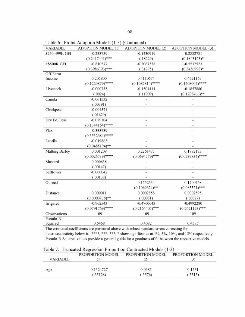
68

Table 6: Probit Adoption Models (1-3) (Continued) VARIABLE ADOPTION MODEL (1) ADOPTION MODEL (2) ADOPTION MODEL (3) $250-499K GFI -0.233759 -0.1430919 -0.2882781 (0.2417441)*** (.18229) (0.1843123)* >$500K GFI -0.810577 -0.2067338 -0.5532523 (0.3986393)*** (.31275) (0.3456998)* Off-Farm Income 0.205800 0.4110674 0.4521169 (0.1220879)**** (0.1082814)**** (0.1208007)**** Livestock -0.000735 -0.1501411 -0.1857880 (.0024) (.11909) (0.1208466)** Canola -0.001532 - - (.00391) - - Chickpeas -0.004571 - - (.01629) - - Dry Ed. Peas -0.079304 - - (0.1344164)**** - - Flax -0.333739 - - (0.3532684)**** - - Lentils -0.019863 - - (0.0485194)** - - Malting Barley 0.001209 0.2261473 0.1982173 (0.0026739)**** (0.0694779)*** (0.0739834)**** Mustard 0.000638 - - (.00147) - - Safflower -0.000042 - - (.00138) - - Oilseed - 0.1552534 0.1700768 - (0.1069624)** (0.085521)*** Distance 0.000011 0.0002858 0.0002595 (0.0000238)** (.00031) (.00027) Irrigated -0.962543 -0.4760643 -0.4992280 (0.0791769)**** (0.2164405)*** (0.2621123)*** Observations 109 109 109 Pseudo-R-Squared 0.6468 0.4082 0.4385 The estimated coefficients are presented above with robust standard errors correcting for heteroscedasticity below it. ****, ***, ***, * show significance at 1%, 5%, 10%, and 15% respectively. Pseudo-R-Squared values provide a general guide for a goodness of fit between the respective models.

Table 7: Truncated Regression Proportion Contracted Models (1-3)

VARIABLE PROPORTION MODEL

(1) PROPORTION MODEL

(2) PROPORTION MODEL

(3) Age 0.1324727 0.0685 0.1531 (.35128) (.3576) (.3515)

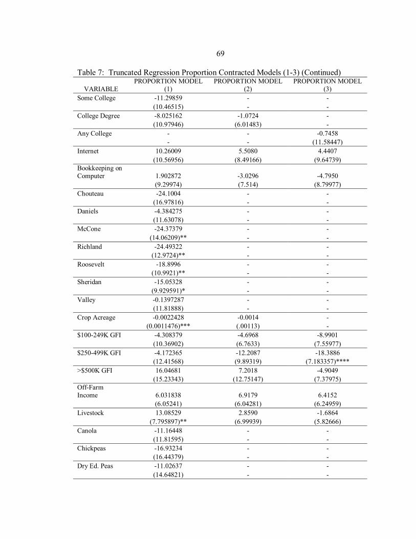
69

Table 7: Truncated Regression Proportion Contracted Models (1-3) (Continued)

VARIABLE PROPORTION MODEL

(1) PROPORTION MODEL

(2) PROPORTION MODEL

(3) Some College -11.29859 - - (10.46515) - - College Degree -8.025162 -1.0724 - (10.97946) (6.01483) - Any College - - -0.7458 - - (11.58447) Internet 10.26009 5.5080 4.4407 (10.56956) (8.49166) (9.64739) Bookkeeping on Computer 1.902872 -3.0296 -4.7950 (9.29974) (7.514) (8.79977) Chouteau -24.1004 - - (16.97816) - - Daniels -4.384275 - - (11.63078) - - McCone -24.37379 - - (14.06209)** - - Richland -24.49322 - - (12.9724)** - - Roosevelt -18.8996 - - (10.9921)** - - Sheridan -15.05328 - - (9.929591)* - - Valley -0.1397287 - - (11.81888) - - Crop Acreage -0.0022428 -0.0014 - (0.0011476)*** (.00113) - $100-249K GFI -4.308379 -4.6968 -8.9901 (10.36902) (6.7633) (7.55977) $250-499K GFI -4.172365 -12.2087 -18.3886 (12.41568) (9.89319) (7.183357)**** >$500K GFI 16.04681 7.2018 -4.9049 (15.23343) (12.75147) (7.37975) Off-Farm Income 6.031838 6.9179 6.4152 (6.05241) (6.04281) (6.24959) Livestock 13.08529 2.8590 -1.6864 (7.795897)** (6.99939) (5.82666) Canola -11.16448 - - (11.81595) - - Chickpeas -16.93234 - - (16.44379) - - Dry Ed. Peas -11.02637 - - (14.64821) - -

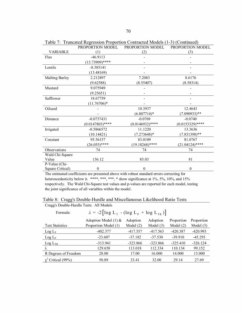
70

Table 7: Truncated Regression Proportion Contracted Models (1-3) (Continued)

VARIABLE PROPORTION MODEL

(1) PROPORTION MODEL

(2) PROPORTION MODEL

(3) Flax -46.9113 - - (13.73909)**** - - Lentils -8.385141 - - (13.48169) - - Malting Barley 2.212897 7.2083 8.6176 (9.62588) (8.55407) (8.58314) Mustard 9.075949 - - (9.25651) - - Safflower 18.67759 - - (11.76706)* - - Oilseed - 10.3937 12.4643 - (6.807714)* (7.090933)** Distance -0.0737431 -0.0769 -0.0740 (0.0147803)**** (0.0146932)**** (0.0153329)**** Irrigated -0.5866572 11.1220 13.3636 (10.14421) (7.273648)* (7.831398)** Constant 95.56157 83.0109 81.0767 (26.055)**** (19.18268)**** (21.04124)**** Observations 74 74 74 Wald Chi-Square Value 136.12 85.03 81 P-Value (Chi-Square Critical) 0 0 0 The estimated coefficients are presented above with robust standard errors correcting for heteroscedasticity below it. ****, ***, ***, * show significance at 1%, 5%, 10%, and 15% respectively. The Wald Chi-Square test values and p-values are reported for each model, testing the joint significance of all variables within the model.

Table 8: Cragg's Double-Hurdle and Miscellaneous Likelihood Ratio Tests

Cragg's Double-Hurdle Tests: All Models Formula:

Adoption Model (1) & Adoption Adoption Proportion Proportion Test Statistics Proportion Model (1) Model (2) Model (3) Model (2) Model (3) Log LT -402.377 -417.557 -417.563 -420.387 -420.993 Log LP -23.607 -37.182 -37.530 -39.910 -45.293 Log LTR -313.941 -323.866 -323.866 -325.410 -326.124 λ 129.658 113.018 112.334 110.134 99.152 R Degrees of Freedom 28.00 17.00 16.000 14.000 13.000 χ2 Critical (99%) 50.89 33.41 32.00 29.14 27.69

[ ]T P TR = -2 log L - (log L + log L )λ

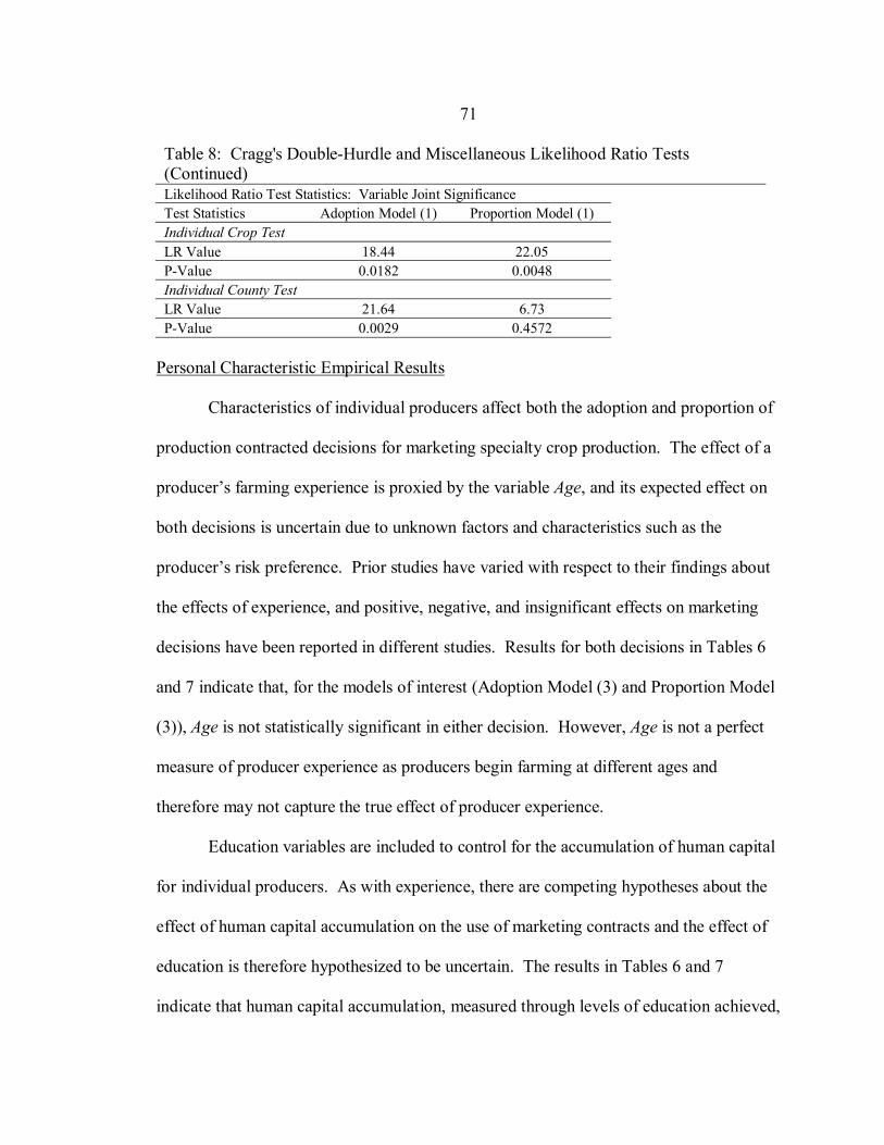
71

Table 8: Cragg's Double-Hurdle and Miscellaneous Likelihood Ratio Tests (Continued) Likelihood Ratio Test Statistics: Variable Joint Significance Test Statistics Adoption Model (1) Proportion Model (1) Individual Crop Test LR Value 18.44 22.05 P-Value 0.0182 0.0048 Individual County Test LR Value 21.64 6.73 P-Value 0.0029 0.4572

Personal Characteristic Empirical Results Characteristics of individual producers affect both the adoption and proportion of

production contracted decisions for marketing specialty crop production. The effect of a

producer�s farming experience is proxied by the variable Age, and its expected effect on

both decisions is uncertain due to unknown factors and characteristics such as the

producer�s risk preference. Prior studies have varied with respect to their findings about

the effects of experience, and positive, negative, and insignificant effects on marketing

decisions have been reported in different studies. Results for both decisions in Tables 6

and 7 indicate that, for the models of interest (Adoption Model (3) and Proportion Model

(3)), Age is not statistically significant in either decision. However, Age is not a perfect

measure of producer experience as producers begin farming at different ages and

therefore may not capture the true effect of producer experience.

Education variables are included to control for the accumulation of human capital

for individual producers. As with experience, there are competing hypotheses about the

effect of human capital accumulation on the use of marketing contracts and the effect of

education is therefore hypothesized to be uncertain. The results in Tables 6 and 7

indicate that human capital accumulation, measured through levels of education achieved,

72

is statistically significant and positively related to the adoption decision but not

statistically significant in the contracted proportion of production decision. The results in

Table 6 indicate that the effects of having a college degree, College Degree, in Adoption

Model (2) is only statistically significant at the 15 percent level, but the variable Any

College, in Adoption Model (3), is statistically significant at the one percent level and the

marginal effect is larger. Holding other explanatory variables at their means, a producer

who attended or graduated from college is just over 60 percent more likely (.6047) to

adopt marketing contracts than producers that have not attended or graduated from

college. These results are similar to findings reported in previous studies which

hypothesized that producers with higher levels of human capital are more successful at

using and understanding marketing contracts (Fletcher and Terza 1986; Goodwin and

Schroeder 1994; Musser et al. 1996; Katchova and Miranda 2004). The results are

inconsistent with the hypothesis that producers with higher levels of education are less

risk-averse and less willing to adopt risk-reducing marketing strategies (Shapiro and

Brorsen 1988). Producers with higher levels of education, having attended college, are

significantly more likely to adopt marketing contracts, but the effect of human capital

accumulation does not significantly affect how much production a producer is likely to

contract.

The willingness of a producer to adopt a new technology is proxied by the dummy

variables Internet and Bookkeeping on Computer. Previous studies have not attempted to

control for technology adoption with these specific variables, but, in general, have

hypothesized that technology adoption is likely to be positively related to the adoption of

73

other new technologies (Goodwin and Schroeder 1994). Therefore, it was expected that

producers willing to adopt the internet and bookkeeping methods to manage their farms

would be willing to adopt marketing contracts and contract a higher proportion of their

production. The results in Tables 6 and 7 do not support this hypothesis as the parameter

estimates for these variables are negative and statistically significant. The marginal

effect of Bookkeeping on Computer is also relatively large as producers adopting

bookkeeping methods on the computer are approximately 17 percent (-.1667) less likely

to adopt marketing contracts than those who do not adopt these methods. The variable

Internet is not significantly related to the adoption decision, and neither variable is

significantly related to the proportion of production to contract decision. Internet

adoption may be capturing technology adoption for personal use rather than farm use and

the use of bookkeeping on the computer may not be a good measure of technology

adoption or may be capturing other unidentified effects of other personal characteristics.

Farm-Specific Characteristic Empirical Results The geographic location of the farming operation may affect marketing decisions

by capturing geographic-specific effects such as proximity to buyers and the number of

buyers in a particular geographic area. Multicollinearity problems precluded the use of

individual county-specific dummy variables. Likelihood ratio tests of the joint

significance of the county variables, reported in Table 8, indicate that while the null

hypothesis that the variables are not jointly significant is rejected for the adoption

decision, it is not rejected for the proportion of production contracted decision.

74

Therefore, geographical categorical variables were included in the subsequent adoption

models with producers in the northeast region, Northeast, serving as the base dummy

variable category29. Results in Table 6 indicate that producers in the northcentral region,

Northcentral, are not significantly more likely to adopt contracts than producers in the

northeast region. Producers in the southcentral region, Southcentral, are approximately

15 percent (.1533) more likely to adopt marketing contracts than producers in the

northeast region, but this result is only statistically significant at the 15 percent level30.

These results may be capturing a measure of the relative thinness of the spot cash market

in various regions in Montana, as regions with fewer locations or buyers of specialty crop

production in the spot cash market are considered thin markets. Thin markets are

hypothesized to have a higher use of marketing contracts, and therefore the results

indicate that the southcentral region may be a relatively thinner market than the northeast

region.

The size of an individual farm, in acres, is accounted for by the variable Crop

Acreage which is included to capture economies of size effects on the use of marketing

contracts. Previous studies have found farm size to be positively related to the use of

marketing contracts (Fletcher and Terza 1986; Shapiro and Brorsen 1988; Goodwin and

29 A likelihood ratio test indicated that the individual county variables contained more information than the regional variables in the contract adoption model. However, as noted above, problems with multicollinearity ultimately precluded the use of the individual county variables. 30 An additional survey of specialty crop buyers in Montana, North Dakota, Alberta, and Sasketchewan conducted in collaboration with Dr. Vincent H. Smith and Dr. James B. Johnson, of Montana State University�s Department of Agricultural Economics & Economics. The survey provided thirteen specific contracts used to purchase specialty crop production. The contracts all contained similar provisions, and some buyers utilized only one contract to purchase more than one specific specialty crop. Therefore, county, regional, and crop-specific variables may not be capturing inherent differences in the structure of the contracts themselves, and are more likely to be picking up actual characteristics of the crop or geographic area.

75

Schroeder 1994; Sartwelle et al. 2000), but one study found farm size not to be

statistically significant (Katchova and Miranda 2004). Results in Tables 6 and 7 are

similar to those reported in previous studies which found economies of size in marketing

contract adoption, but farm size does not have a significant effect on the contracted

proportion of production. Increasing Crop Acreage by 1,000 acres increases the

probability of marketing contract adoption by approximately 12 percent (.1234), holding

other explanatory variables at their means.

Gross farm income (GFI), a second measure of farm size, is accounted for by the

dummy variables $100-249K GFI, $250-499K GFI, and >$500K GFI. As with farm

size, GFI may serve as a proxy for farm size, but income variables may also control for

increasing producer wealth. Producers may become less risk-averse as their wealth

increases, and therefore, a priori, the effects of gross farm income on contracting

decisions are unclear. Previous studies have reported that farms with higher gross farm

incomes are more likely to adopt marketing contracts (Asplund et al. 1989; Edelman et al.

1990; Katchova and Miranda 2004), but some found that the contracted proportion of

production was negatively related to gross farm income (Musser et al. 1996). In Tables 6

and 7, only two of the gross farm income variables, $250-499K GFI and >$500K GFI,

are statistically significant (at the 15 percent level) and negatively related to the adoption

decision. A producer with $250-499K GFI is approximately 29 percent (-.2883) less

likely to adopt marketing contracts than producers with $0-99K GFI, while a producer

with >$500K GFI is approximately 55 percent (-.5532) less likely to adopt marketing

contracts than producers with $0-99K GFI. In addition, $250-499K GFI is the only

76

statistically significant GFI variable negatively related to the proportion of production

contracted decision. A producer with $250-499K GFI contracts approximately 18

percent (-18.3886) less production than a producer with $0-99K GFI. These results are

inconsistent with the hypotheses that gross farm income serves as an indicator of

economies of size in the use of marketing contracts, but the results are similar to those

reported with previous studies that have reported that producers with higher income are

less risk-averse (Musser et al. 1996).

Two additional income variables control for farm diversification by indicating

whether or not a farm receives income from off-farm sources, Off-Farm Income, or from

the sale of livestock, Livestock. Previous studies have reported that farms with additional

sources of income, or those that are not specialized in grain production, are less likely to

adopt or use marketing contracts (Edelman et al. 1990; Musser et al. 1996; McLeay and

Zwart 1998; Sartwelle et al. 2000; Katchova and Miranda 2004). Similar results are

reported here. The variable Livestock is statistically significant and the results indicate

that producers with income from the sale of livestock are approximately 19 percent (-

.1858) less likely to adopt marketing contracts than producers without income from

livestock. However, the adoption of marketing contracts is positively related to Off-Farm

Income, a finding that is inconsistent with results from previous studies. The contracted

proportion of production decision is not significantly related to either Livestock or Off-

Farm Income. Off-Farm Income and Livestock are not perfect proxies for farm

diversification, and therefore the results of each variable may be capturing other

information.

77

Crop-Specific Characteristic Empirical Results One important aspect of this study relative to previous studies is the attempt to

explain the use of contracts in terms of characteristics specific to individual specialty

crops. Characteristics of an individual crop may also significantly affect marketing

decisions through capturing various crop-specific effects such as quality requirements or

other specific needs of the buyers of individual crops. As with county-specific variables,

correlation problems precluded the use of individual crop-specific dummy variables.

Likelihood ratio tests for the joint significance of the crop-specific variables, reported in

Table 8, indicate that the null hypothesis that the variables are not jointly significant is

rejected for both the adoption and proportion contracted decisions. Therefore, crop-

related categorical variables were included in the subsequent adoption models.

The results indicate that relative to the base category Pulses, both Oilseeds and

Malting Barley are statistically significantly and positively related to the adoption

decision. Only Oilseeds are statistically significantly and positively related to the

proportion of production to contract decision. Oilseeds are approximately 17 percent

(.1701) more likely to be contracted than Pulses; Malting Barley is approximately 20

percent (.1982) more likely to be contracted than Pulses. In addition, the contracted

proportion of Oilseeds production is approximately 12 percent (12.4643) higher than the

proportion of Pulses production. These results suggest that crops such as Pulses are less

likely to be contracted than other crops and, if contracted, are contracted in lower

proportions than other crops. In addition to the geographic location variables, crop-

78

specific variables may be capturing the relative thinness of the spot cash market for

individual crops or categories of crops. Crops with fewer buyers or locations for delivery

of production in the spot cash market are considered thin markets, and thin markets are

hypothesized to have a higher use of marketing contracts due to fewer opportunities to

deliver production in the spot cash market. Thus, the results indicate that there may be

more buyers in the spot cash market of pulse crops than oilseed crops and malting barley

and the pulse crop market is not as thin as the market for oilseeds and malting barley31.

The distance to the market for a specific specialty crop is proxied by the variable

Distance. No distinctions can be made between the difference in distances between

production marketed with contracts and production sold in the spot cash market, thus the

effects of distance were uncertain. Previous results indicated that distance is not a

significant predictor of contract use (Sartwelle et al. 2000). However, the results in

Tables 6 and 7 indicate that the adoption decision is not significantly related to Distance,

but the contracted proportion of production is significantly and negatively related to

Distance. As the distance to the market for contracted production increases by one

hundred miles, the overall proportion of production contracted decreases by

approximately seven percent (-.074). Therefore, for producers who contract, being

further away from the market decreases the proportion of production that will be

contracted. This result is consistent with the rationale that transportation costs increase as

31 The North Dakota Dry Pea and Lentil Association listed 53 pulse crop buyers in a region encompassing North Dakota, Minnesota, Saskatchewan, California, and Manitoba. The Agriculture and Agri-Food Department of Canada listed five oilseed crushing facilities in a region encompassing North Dakota, Manitoba, and Montana. Thus, it appears that the market for oilseeds is thinner than the market for pulse crops for producers in Montana.

79

the distance to the market increases, and therefore a lower proportion of production will

be marketed under contract.

The level of production costs, yield variability, and buyer preferences for a

specific quality of a specialty crop are proxied by measuring whether a crop is irrigated

or not through the dummy variable, Irrigated. Irrigated crops are hypothesized to be

positively related to both contracting decisions as production costs are higher for irrigated

crops, the probability of producers defaulting on contracts is lower due to less yield

variability with irrigated crops. In addition, buyers may seek to purchase irrigated

specialty crop production through contracts due to increased yield consistency and

quality. The results in Tables 6 and 7 indicate that the variable Irrigated is statistically

significant in both the adoption decision and the contracted proportion of production

decision. However, the sign on the coefficient for Irrigated in the adoption decision is

negative while the sign on the coefficient for Irrigated in the proportion contracted is

positive. Irrigated crops are approximately 50 percent (-.4992) less likely to be

contracted than dryland crops, but among contracted crops, approximately 13 percent

(13.364) more of production is contracted for irrigated crops than for dryland crops.

Therefore, if a crop is irrigated, the probability of marketing contract adoption decreases,

but for those that adopt marketing contracts, an irrigated crop increases the proportion of

production contracted. This is consistent with the hypothesis that the risk of default on

the contract matters for marketing decisions made by individual producers and the

hypothesis that buyers of specialty crops may seek to purchase more irrigated production.

80

Summary

This chapter has described the empirical analysis of how personal, farm-specific,

and crop-specific characteristics affect the adoption of marketing contracts and the

decision of what proportion of production to contract. Cragg�s double-hurdle likelihood

ratio test provides empirical evidence that estimating each decision independently is

appropriate. Therefore, probit models were estimated to explain the adoption decision

while separate truncated regressions were estimated to explain the decision about what

proportion of production to contract.

Adoption of marketing contracts is significantly affected by a wide variety of

personal, farm-specific, and crop-specific characteristics. Producers with higher levels of

human capital, Any College, are approximately 60 percent more likely to adopt contracts

than producers with lower levels of human capital. Also, producers of Oilseeds and

Malting Barley are approximately 17 and 20 percent more likely to adopt marketing

contracts than producers of Pulses respectively, providing evidence that the spot cash

markets for oilseeds and malting barley is thinner than the spot cash market for pulse

crops. Economies of size are supported in the adoption decision as producers with more

cropland acres, Crop Acreage, are more likely to adopt marketing contracts. Diversified

farms receiving receipts of income from the sale of livestock, Livestock, are

approximately 19 percent less likely to adopt marketing contracts, supporting the

hypothesis that farms more specialized in crop production are more likely to adopt

marketing contracts. Gross farm income variables, $250-499K GFI and >$500K GFI,

81

are only statistically significant at the 15 percent level, and negatively related to the

adoption decision. These findings are inconsistent with the hypothesis that income serves

as a proxy for economies of size but provide support for the decreasing risk aversion

hypothesis.

Producers operating in the southcentral geographic region, Southcentral, are more

likely to adopt marketing contracts than producers in the northeast geographic region

providing evidence that the spot cash market is thinner in the southcentral region, but this

result is only significant at the fifteen percent level. The adoption of bookkeeping on the

computer, Bookkeeping on Computer, and irrigated crops, Irrigated, both significantly

decreased the probability of marketing contract adoption which was inconsistent with the

hypothesized effects of each. In addition, receiving off-farm income, Off-Farm Income,

significantly increased the probability of adoption which was contrary to expectations as

well. Bookkeeping on Computer, Irrigated, and Off-Farm Income may be capturing other

characteristics due to the fact that they are not perfect proxies for technology adoption,

value of production, and income diversification respectively.

The decision of what proportion of specialty crop production to market with

contracts is significantly affected by relatively few farm and crop-specific characteristics

and personal characteristics are all insignificant. Oilseeds are contracted in higher

proportions, approximately 12 percent, than Pulses. One measure of gross farm income,

$250-499K GFI, supports the reduction in risk aversion hypothesis that higher levels of

income reduce a producer�s level of risk aversion and therefore they utilize risk-reducing

mechanisms such as contracting less frequently. A crop that is irrigated, Irrigated, is

82

contracted in significantly higher proportions than contracted non-irrigated crops,

supporting the hypothesis that the probability of contract default by producers is lower

with irrigated production due to decreased yield variability and also supporting the

hypothesis that buyers may seek to purchase irrigated production with contracts. Thus,

irrigated crops will be contracted in higher proportions. As the distance from the

contracting market, Distance, increases, crops are contracted in lower proportions

suggesting that the increased transportation costs per unit of production are important in

how producers market their production.

Overall, a wider variety of personal, farm-specific, and crop-specific variables

affect the marketing contract adoption decision, while only a small number of farm-

specific and crop-specific variables affect the decision of what proportion of production

to contract. This implies that once the decision to contract has been made, producers

decide what proportion to contract based on only a few farm and crop-specific

characteristics.

83

CHAPTER 7

CONCLUSION

The purpose of this study has been to examine why the use of contracts as

marketing mechanisms varies across producers and crops. Contract use is affected by

personal, farm-specific, and crop-specific characteristics. Contract use by specialty crop

producers is examined using data obtained from a non-random sample of 89 farmers

located in eight Montana counties. The survey gathered information on operator, farm-

specific, and crop-specific characteristics. The effects of crop-specific characteristics on

contracting decisions have not been examined in previous studies.

Two separate and independent marketing decisions concerning contract use are

examined. The first is the decision about whether or not to contract at all. If the expected

utility of profits obtained from marketing at least a portion of production with marketing

contracts is greater than the expected utility of profits from utilizing only the spot cash

market, then marketing contracts will be adopted. Producers who adopt marketing

contracts must then decide what proportion of their output to market under contract and

what proportion to market in the spot cash market. The double-hurdle framework allows

each of these decisions to be affected in different ways by the same or a different set of

characteristics. Cragg�s double-hurdle likelihood ratio tests provide support for the two-

stage approach to modeling the adoption and proportion of production contracted

decisions.

84

The results from this study indicate that the marketing contract adoption decision

is affected by the personal characteristics of the farmer, but the contracted proportion of

production decision is not affected in a statistically significant way by those

characteristics. Neither decision is significantly related to the proxy for years of

producer experience, although the proxy variable Age may not perfectly capture the true

effect of producer experience. However, producers with higher levels of human capital

accumulation, as measured by a producer�s highest level of education achieved, were

found to be more likely to adopt marketing contracts. This may be because producers

with higher levels of human capital have lower costs of understanding and interpreting

terms of contracts, which increases contract adoption.

The adoption of marketing contracts and the contracted proportion of production

decisions are both hypothesized to be positively related to a producer�s willingness to

adopt new technologies. Parameter estimates for the variables used to proxy for this

characteristic, adoption of the internet and methods of bookkeeping on the computer, did

not support this hypothesis, but these variables may be capturing other personal or farm-

related characteristics because they are not perfect proxies for willingness to adopt new

technology.

Both the contract adoption and the proportion of production to contract decisions

were found to be significantly related to specific characteristics of a farm�s operations.

Economies of size, in terms of total crop acreage, are supported in the adoption decision

as producers with more cropland acres are more likely to adopt marketing contracts.

However, as gross farm income increases, the probability of marketing contract adoption

85

and the proportion of production contracted both decline. These two results are not

consistent with the economies of size hypothesis, but do provide support for the

hypothesis that producers with higher levels of gross farm income are less risk-averse and

thus less likely to adopt risk-reducing mechanisms such as marketing contracts.

Other variables that control for additional sources of farm income and the

geographic location of the farming operation were examined. The results indicate that

farms with livestock operations are less likely to adopt contracting for their specialty crop

production. The decision to adopt contracts was significantly related to county or region-

specific dummy variables, which indicate the geographic location of the farming

operation. However, the decision about what proportion of specialty crop production to

market under contract was not significantly related to these variables. Geographic

variables were included to capture county or regional-specific information and other

random factors such as soil types, weather, and other characteristics that may be

significantly related to the adoption and use of marketing contracts. Including all county-

specific variables provided results which suggested that multicollinearity may be a

problem between county variables and other explanatory variables such as the income-

related variables. Therefore, regional categorical variables were utilized and the results

indicate that producers operating in the southcentral region of Montana are more likely to

adopt marketing contracts than producers in the northeast region. This result suggests

that the spot cash market in the southcentral region may be relatively thinner than the

northeast region.

86

One important contribution of this study is the inclusion of crop-specific variables

to control for crop-related characteristics that influence the adoption and use of marketing

contracts. The inclusion of dummy variables for each crop suggested that

multicollinearity may be a problem between the crop dummy variables and other

explanatory variables. Thus, each crop was allocated to one of three categories: pulses,

oilseeds, and malting barley. The results of this study indicate that oilseed crops and

malting barley are significantly more likely to be contracted than pulse crops, and

producers are significantly more likely to contract higher proportions of their production

of oilseeds than pulse crops. These results indicate that the spot cash market may be

relatively thinner for oilseeds and malting barley compared with pulse crops, as there

may be more buyers of pulse crops in the spot cash market.

A crop that is irrigated is significantly less likely to be contracted than dryland

crops. However, for crops that are contracted, irrigating the crop significantly increased

the proportion of production that is contracted. This provides support to the hypothesis

that irrigated crops have less variability in production and therefore less probability for

default on the contract by the producer, and also that buyers of specialty crops are more

likely to seek to contract for a higher proportion of irrigated production to contract.

The adoption of marketing contracts is not significantly related to the distance

from the market, but the contracted proportion of production is significantly reduced as

the distance to the market increases. This result supports the hypothesis that

transportation costs increase as the distance to the contract market increases, and

therefore a lower proportion of production is contracted.

87

In summary, a variety of personal, farm-specific, and crop-specific characteristics

affect the adoption of marketing contracts. However, a smaller number of farm and crop-

specific characteristics affect the decision about what proportion of production to

contract. This study has examined the role of crop-specific variables in explaining

differences in contracting by crop and has utilized new measures of crop characteristics

such as an indicator variable for irrigation. A new, primary dataset was collected and

utilized to examine contracting among specialty crops. The variables used in this study

to proxy particular characteristics may not have been perfect representations of the

characteristics themselves, and this study was limited to the 109 survey observations in

the dataset of Montana Grain Growers Association Members. Future research would

benefit by extending this study beyond the limited geographic area accounted for in this

study. In addition, variables that more closely proxy the characteristics hypothesized to

affect each marketing decision may increase significance and robustness of the results.

88

REFERENCES CITED

Ackerberg, D. A. and M. Botticini (2000). "The Choice of Agrarian Contracts in Early Renaissance Tuscany: Risk Sharing, Moral Hazard, or Capital Market Imperfections?" Explorations in Economic History 37: 241-257. Ackerberg, D. A. and M. Botticini (2002). "Endogenous Matching and the Empirical Determinants of Contract Form." Journal of Political Economy 110(3): 564-591. Agriculture, U. S. D. o. (1996). Farmers' Use of Marketing and Production Contracts. E. R. Service, Economic Research Service/USDA. AER-747: 1-20. Agriculture, U. S. D. o. (2004). Contracts, Markets, and Prices: Organizing the Production and Use of Agricultural Commodities. E. R. Service, Economic Research Service/USDA. AER-837: 8-23. Allen, D. W. and D. Lueck (1999). "The Role of Risk in Contract Choice." Journal of Law, Economics, and Organization 15(3): 704-736. Arrow, K. J. (1969). The Organization of Economic Activity: Issues Pertinent to the Choice of Market Versus Nonmarket Allocation. The Analysis and Evaluation of Public Expenditure. s. C. United States Joint Economic Committee, 1st Session, United States Government Printing Office. 1: 59-73. Asplund, N. M., et al. (1989). "Farmers' Use of Forward Contracting and Hedging." The Review of Futures Markets 8: 24-37. Bolton, P. and M. Dewatripont (2005). Contract Theory. Cambridge, MA, The MIT Press. Bureau, U. S. C. (2005). Montana County Selection Map. State & County Quickfacts, http://quickfacts.census.gov/qfd/maps/montana_map.html. Cheung, S. N. S. (1969). "Transaction Costs, Risk Aversion, and the Choice of Contractual Arrangements." Journal of Law and Economics 12(1): 23-42. Coase, R. H. (1937). "The Nature of the Firm." Economica 4: 386-405. Cragg, J. G. (1971). "Some Statistical Models for Limited Dependent Variables with Application to the Demand for Durable Goods." Econometrica 39(5): 829-844.

89

Edelman, M. A., et al. (1990). "Use of Selected Marketing Alternatives by Iowa Farmers." Agribusiness 6(2): 121-132. Fletcher, S. M. and J. V. Terza (1986). "Analyzing Farmers' Selection of Available Marketing Alternatives using the Multivariate Probit Model." Canadian Journal of Agricultural Economics 34: 243-252. Goodhue, R. E. (1999). "Input Control in Agricultural Production Contracts." American Journal of Agricultural Economics 81: 616-620. Goodwin, B. K. and T. C. Schroeder (1994). "Human Capital, Producer Education Programs, and the Adoption of Forward-Pricing Methods." American Journal of Agricultural Economics 76(4): 936-947. Greene, W. H. (2000). Econometric Analysis. Upper Saddle River, NJ, Prentice-Hall, Inc. Holmstrom, B. (1979). "Moral Hazard and Observability." The Bell Journal of Economics 10(1): 74-91. Hudson, D. and J. Lusk (2004). "Risk and Transactions Cost in Contracting: Results from a Choice-Based Experiment." Journal of Agricultural and Food Industrial Organization 2(2): 1-17. Hueth, B. and E. Ligon (1999). "Producer Price Risk and Quality Measurement." American Journal of Agricultural Economics 81: 512-524. Hueth, B. and T. Melkonyan (2004). "Identity Preservation, Multitasking, and Agricultural Contract Design." American Journal of Agricultural Economics 86(3): 842-847. Jensen, M. C. and W. H. Meckling (1976). "Theory of the Firm: Managerial Behavior, Agency Costs and Ownership Structure." Journal of Financial Economics 3: 305-360. Johnson, S. R. and K. R. Tefertiller (1964). Estimating the Influence of Diversification on Farm Income Variability, Dryland Row-crop Farms - High Plains of Texas. Texas Agricultural Experiment Station Publication MP-751, Texas A&M University: 1-14. Katchova, A. L. and M. J. Miranda (2004). "Two-Step Econometric Estimation of Farm Characteristics Affecting Marketing Contract Decisions." American Journal of Agricultural Economics 86(1): 88-102. Kennedy, P. (2003). A Guide to Econometrics. Cambridge, MA, The MIT Press.

90

Klein, B., et al. (1978). "Vertical Integration, Appropriable Rents, and the Competitive Contracting Process." Journal of Law and Economics 21(2): 297-326. Lajili, K., et al. (1997). "Farmers' Preferences for Crop Contracts." Journal of Agricultural and Resource Economics 22(2): 264-280. Leffler, K. B. and R. R. Rucker (1991). "Transactions Costs and the Efficient Organization of Production: A Study of Timber-Harvesting Contracts." Journal of Political Economy 99(5): 1060-1087. Liao, T. F. (1994). Interpreting Probability Models: Logit, Probit, and Other Generalized Linear Models. Thousand Oaks, CA, SAGE Publications, Inc. Ligon, E. (2002). Quality and Grading Risk. A Comprehensive Assessment of the Role of Risk in U.S. Agriculture. R. E. Just and R. D. Pope. Norwell, Massachusetts, Kluwer Academic Publishers: 353-369. Ligon, E. (2003). "Optimal Risk in Agricultural Contracts." Agricultural Systems 75: 265-276. Lin, T.-F. and P. Schmidt (1984). "A Test of the Tobit Specification Against an Alternative Suggested by Cragg." Review of Economics and Statistics 66: 174-177. McLeay, F. and T. Zwart (1998). "Factors Affecting Choice of Cash Sales Versus Forward Marketing Contracts." Agribusiness 14(4): 299-309. Morrison-Paul, C. J., et al. (2004). "Productivity Economies, and Efficiency in U.S. Agriculture: A Look at Contracts." American Journal of Agricultural Economics 86(5): 1308-1314. Musser, W. N., et al. (1996). "Risk and Grain Marketing Behavior of Large-Scale Farmers." Review of Agricultural Economics 18(1): 65-77. Sandmo, A. (1971). "On the Theory of the Competitive Firm Under Price Uncertainty." The American Economic Review 61(1): 65-73. Sartwelle, I., James , et al. (2000). "The Effect of Personal and Farm Characteristics Upon Grain Marketing Practices." Journal of Agricultural and Applied Economics 32(1): 95-111. Schrader, L. F. (1986). "Responses to Forces Shaping Agricultural Marketing: Contracting." American Journal of Agricultural Economics 68(5): 1161-1166.

91

Shapiro, B. I. and B. W. Brorsen (1988). "Factors Affecting Farmers' Hedging Decisions." North Central Journal of Agricultural Economics 10(2): 145-153. Stiglitz, J. E. (1974). "Incentives and Risk Sharing in Sharecropping." The Review of Economic Studies 41(2): 219-255. Vukina, T. and P. Dubois (2004). "Grower Risk Aversion and the Cost of Moral Hazard in Livestock Production Contracts." American Journal of Agricultural Economics 86(3): 835-841. Vukina, T. and A. Levy (2004). "The League Composition Effect in Tournaments with Heterogeneous Players: An Empirical Analysis of Broiler Contracts." Journal of Labor Economics 22(2): 353-377. Ward, C., et al. (2000). "Contracting in the U.S. Pork and Beef Industries: Extent, Motives, and Issues." Canadian Journal of Agricultural Economics 48(4): 629-641. Williamson, O. E. (1979). "Transaction-Cost Economics: The Governance of Contractual Relations." Journal of Law and Economics 22: 233-261. Williamson, O. E. (1981). "The Modern Corporation: Origins, Evolution, Attributes." Journal of Economic Literature 19(4): 1537-1568. Williamson, O. E. (1991). "Comparative Economic Organization: The Analysis of Discrete Structural Alternatives." Administrative Science Quarterly 36(2): 269-296. Wolf, S., et al. (2001). "Policing Mechanisms in Agricultural Contracts." Rural Sociology 66(3): 359-381.

92

APPENDICES

93

APPENDIX A

EMPIRICAL LITERATURE REVIEW TABLE

94

Table 9: Empirical Literature Review Table

Authors Data Utilized Estimation Technique Key Findings

Fletcher and Terza (1986)

Survey (1982 Georgia wheat

producers)

Multivariate Probit

Educated farmers of large operations with storage facilities and who use associations for price information are more likely to use contracts. Age,

diversification, and full versus part-time farming had no statistically significant impact on contract use.

Shapiro and Brorsen (1988)

Survey (1985 Top Farmer Crop Workshop)

Tobit

Differences in the beliefs of the futures markets� ability to provide income stability were the most important in determining the level of

hedging. Highly leveraged farmers forward contracted much more than they hedged. Education levels and class participation didn�t affect

hedging differences among producers.

Asplund, Forster, and Stout (1989)

Survey Panel (1989 Ohio farm

households) Logit

Economies of size exist in the use of marketing tools indicating a minimum level of gross sales which must exist to justify the costs of

contracting (or hedging). Using computers and consulting services as well as participation in farm organizations are actions of searching that

increase contract use. Full-time operators of large farms tend to be risk-averse and seek to use risk-reduction strategies like forward pricing.

Operators of smaller farms with financial leverage tend not to use forward pricing tools.

Edelman, Schmiesing, and Olsen

(1990)

Survey (1988 Iowa Farm

Finance Survey) Logit

Larger, specialized farm operations are more likely to use forward pricing mechanisms and there are complementarities in the use of other various forward pricing alternatives suggesting that education efforts

may increase the use of multiple forward pricing mechanisms.

Goodwin and Schroeder

(1994)

Survey (1992 Kansas farms)

Probit and Tobit

Adoption of forward pricing decreases with increased experience, but increases with farm size, crop intensity, input intensity, leverage, and education. The most important result, in the authors� opinions, is that participation in marketing and risk management educational programs

increases adoption.

Musser, Patrick, and

Eckman (1996)

Survey (1993 Top Farmer Crop Workshop)

Tobit

Age and education had short-run effects on using contracts but no long-run effects. Size of the farm had a significant negative impact

suggesting as the farm size increased, contracting was used less often for the sample of large farmers. Leveraged farmers were more likely to

contract and attitude toward losses was significant in the long-run.

McLeay and Zwart (1998)

Survey (New Zealand crop

farmers) Logit

The percent of farm area devoted to a crop was positively associated with forward contract use and products that require high levels of

physical capital to grow or harvest are more likely to be sold using contracts. No evidence found for contracts prevailing in perishable

crops or those that have high levels of price variability.

Sartwelle et al. (2000)

Survey (Kansas, Iowa, and Texas

producers)

Tobit and Multinomial

Logit

Use of contracts is positively affected by geographic location, average crop acreage, specialization in grain enterprises, and the use of on-farm

storage. There is no impact of grain marketers� attitudes toward managing price risk upon their marketing practice decisions. The use of

crop insurance has a positive relationship with the use of forward contracts.

Katchova and Miranda (2004)

Survey (1999 USDA's NASS ARMS Study)

Probit, Tobit, Poisson, and

Logit

Personal and farm characteristics affect the adoption decision and the quantity, frequency, and contract type decisions in very different ways. Specialized farmers contract more frequently, and education programs and advisory services increase adoption of contracts. Well-educated

farmers on large farms that use written marketing plans, advisory services, and futures are more likely to adopt contracts. Personal and farm characteristics mostly affect the adoption decision over the other

decisions. Personal and farm characteristics that increase probability of adoption do not necessarily increase quantity, frequency, or contract

types.

95

APPENDIX B

SAMPLE LETTERS AND SURVEY FORMS

96

INITIAL SURVEY LETTER (Montana Grain Growers Association Letterhead) Date Dear Producer, Enclosed you will find a one-page survey concerning the production of specialty agricultural crops. The Montana Grain Growers Association and the Department of Agricultural Economics and Economics at Montana State University are collaborating to implement a survey project on the production and marketing of specialty grains and oilseeds in Montana. We would like to ask you to respond to the following questionnaire. The information in this survey simply addresses whether or not you produce specialty crops. We would like to ask you how many acres of your operation have been planted to each of several specialty crops over the past three years and whether or not you were able to harvest those acres. All responses will be held as strictly confidential and information will be presented in summary with similar responses from other producers. Any information you could provide will greatly facilitate our understanding of the role of alternative crops in Montana farm operations. Please take just a few moments to answer the survey questions as completely as possible and return your answers in the enclosed postage-paid envelope. If you have produced any of the crops listed in the following survey, it would be especially helpful to this project if you would be willing to participate in a more detailed follow-up survey concerning the marketing and contracting of these crops. If you are willing to participate in the follow-up marketing survey, please respond to questions 2 and 3 of the survey. Please note that we are utilizing this two-stage approach to minimize any inconvenience you may incur in participating in this project. We at Montana Grain Growers and Montana State University appreciate your time and efforts to make this project a success, and we look forward to receiving your completed survey. This survey is being administered by the Montana Grain Growers Association to ensure that no other entity will have access to your mailing address. With Best Wishes and Many Thanks, Richard Owen Vince Smith Executive Vice-President Professor Montana Grain Growers Association Montana State University

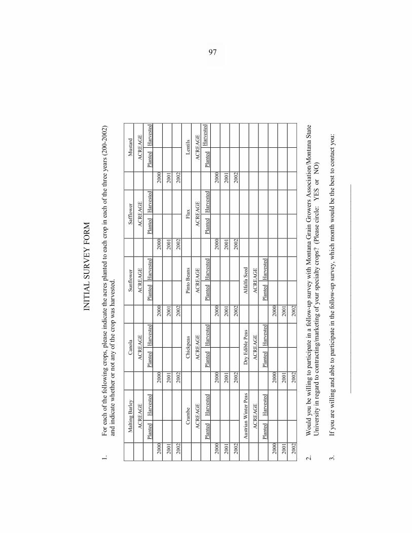
IN

ITIA

L SU

RVEY

FO

RM

1.

Fo

r eac

h of

the

follo

win

g cr

ops,

plea

se in

dica

te th

e ac

res p

lant

ed to

eac

h cr

op in

eac

h of

the

thre

e ye

ars (

200-

2002

) an

d in

dica

te w

heth

er o

r not

any

of t

he c

rop

was

har

vest

ed.

Mal

ting

Bar

ley

C

anol

a

Sunf

low

er

Sa

fflo

wer

Mus

tard

A

CR

EAG

E

AC

REA

GE

A

CR

EAG

E

AC

REA

GE

A

CR

EAG

E

Pl

ante

d H

arve

sted

Plan

ted

Har

vest

ed

Plan

ted

Har

vest

ed

Plan

ted

Har

vest

ed

Plan

ted

Har

vest

ed

2000

2000

2000

2000

2000

2001

2001

2001

2001

2001

2002

2002

2002

2002

2002

C

ram

be

C

hick

peas

Pint

o B

eans

Flax

Lent

ils

A

CR

EAG

E

AC

REA

GE

A

CR

EAG

E

AC

REA

GE

A

CR

EAG

E

Pl

ante

d H

arve

sted

Plan

ted

Har

vest

ed

Plan

ted

Har

vest

ed

Plan

ted

Har

vest

ed

Plan

ted

Har

vest

ed

2000

2000

2000

2000

2000

2001

2001

2001

2001

2001

2002

2002

2002

2002

2002

A

ustri

an W

inte

r Pea

s

Dry

Edi

ble

Peas

Alfa

lfa S

eed

A

CR

EAG

E

AC

REA

GE

A

CR

EAG

E

Pl

ante

d H

arve

sted

Plan

ted

Har

vest

ed

Plan

ted

Har

vest

ed

2000

2000

2000

2001

2001

2001

2002

2002

2002

2.

W

ould

you

be

will

ing

to p

artic

ipat

e in

a fo

llow

-up

surv

ey w

ith M

onta

na G

rain

Gro

wer

s Ass

ocia

tion/

Mon

tana

Sta

te

Uni

vers

ity in

rega

rd to

con

tract

ing/

mar

ketin

g of

you

r spe

cial

ty c

rops

? (P

leas

e ci

rcle

: Y

ES o

r N

O)

3.

If

you

are

will

ing

and

able

to p

artic

ipat

e in

the

follo

w-u

p su

rvey

, whi

ch m

onth

wou

ld b

e th

e be

st to

con

tact

you

:

___

____

____

____

____

____

____

____

____

____

____

____

____

____

____

___

97

98

FOLLOW-UP SURVEY LETTER (Montana Grain Growers Association Letterhead) September 29, 2003 Dear _________________(Producer), Thank you for volunteering to participate in this follow-up survey concerning the marketing and contracting of specialty crops. Enclosed you will find two forms. First, please complete the yellow form. The yellow form pertains to your overall farm/ranch operation. Next, you will see that there are several green forms. Please complete a green form for each OTHER (SPECIALTY) crop that you listed as planted in 2003 on question two (2) of the yellow form. Please complete a green form for OTHER (SPECIALTY) crops grown in any or all of the years from 2000-2003 (please indicate year grown). Please return the completed yellow and green forms in the enclosed pre-paid envelope. The Montana Grain Growers Association and Montana State University would like to emphasize that all responses are strictly confidential. The information you provide will be presented in summary form with responses from other producers and will greatly facilitate the understanding of the importance of marketing contracts to Montana alternative crop producers. We sincerely appreciate your time and effort to make this project a success. We look forward to receiving your completed forms. This survey is being administered by the Montana Grain Growers Association to ensure that no other entity has access to your mailing address. Please place the survey in the mail no later than October 10, 2003. Thanks, Richard Owen Executive Vice-President Montana Grain Growers Association

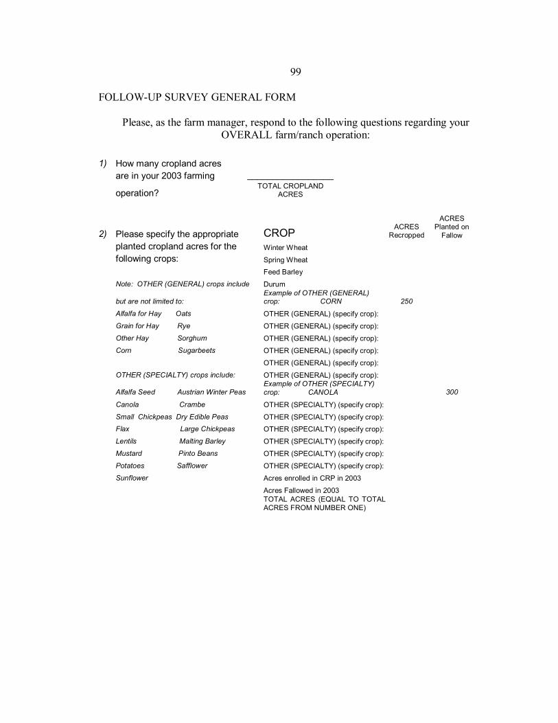
99

FOLLOW-UP SURVEY GENERAL FORM

Please, as the farm manager, respond to the following questions regarding your OVERALL farm/ranch operation:

2) Please specify the appropriate CROP ACRES

Recropped

ACRES Planted on

Fallow planted cropland acres for the Winter Wheat following crops: Spring Wheat Feed Barley Note: OTHER (GENERAL) crops include Durum

but are not limited to: Example of OTHER (GENERAL) crop: CORN 250

Alfalfa for Hay Oats OTHER (GENERAL) (specify crop): Grain for Hay Rye OTHER (GENERAL) (specify crop): Other Hay Sorghum OTHER (GENERAL) (specify crop): Corn Sugarbeets OTHER (GENERAL) (specify crop): OTHER (GENERAL) (specify crop): OTHER (SPECIALTY) crops include: OTHER (GENERAL) (specify crop):

Alfalfa Seed Austrian Winter Peas Example of OTHER (SPECIALTY) crop: CANOLA 300

Canola Crambe OTHER (SPECIALTY) (specify crop): Small Chickpeas Dry Edible Peas OTHER (SPECIALTY) (specify crop): Flax Large Chickpeas OTHER (SPECIALTY) (specify crop): Lentils Malting Barley OTHER (SPECIALTY) (specify crop): Mustard Pinto Beans OTHER (SPECIALTY) (specify crop): Potatoes Safflower OTHER (SPECIALTY) (specify crop): Sunflower Acres enrolled in CRP in 2003 Acres Fallowed in 2003

TOTAL ACRES (EQUAL TO TOTAL ACRES FROM NUMBER ONE)

1) How many cropland acres are in your 2003 farming _________________

operation? TOTAL CROPLAND

ACRES

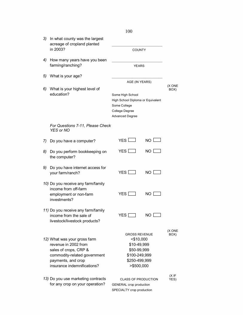
100

3) In what county was the largest acreage of cropland planted ______________________________________ in 2003? COUNTY 4) How many years have you been ______________________________________ farming/ranching? YEARS 5) What is your age? ______________________________________ AGE (IN YEARS)

6) What is your highest level of (X ONE BOX)

education? Some High School High School Diploma or Equivalent Some College College Degree Advanced Degree

For Questions 7-11, Please Check YES or NO

7) Do you have a computer? YES NO 8) Do you perform bookkeeping on YES NO the computer? 9) Do you have internet access for your farm/ranch? YES NO 10) Do you receive any farm/family income from off-farm employment or non-farm YES NO investments?

11) Do you receive any farm/family

income from the sale of YES NO

livestock/livestock products?

GROSS REVENUE (X ONE BOX)

12) What was your gross farm <$10,000 revenue in 2002 from $10-49,999 sales of crops, CRP & $50-99,999 commodity-related government $100-249,999 payments, and crop $250-499,999 insurance indemnifications? >$500,000

13) Do you use marketing contracts CLASS OF PRODUCTION (X IF YES)

for any crop on your operation? GENERAL crop production SPECIALTY crop production

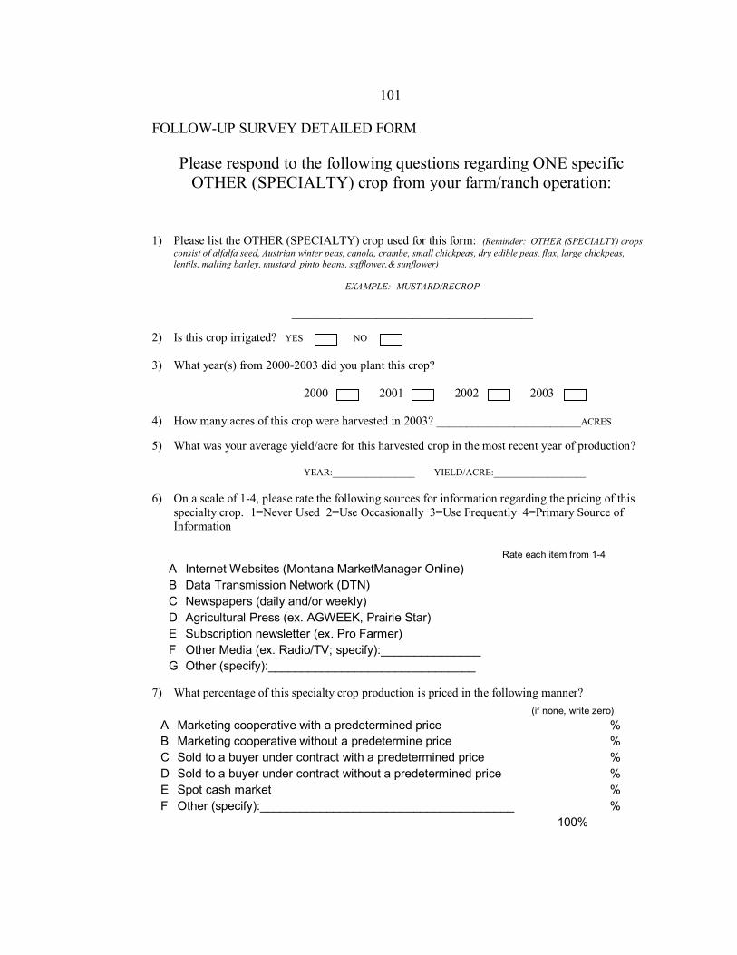
101

FOLLOW-UP SURVEY DETAILED FORM

Please respond to the following questions regarding ONE specific

OTHER (SPECIALTY) crop from your farm/ranch operation: 1) Please list the OTHER (SPECIALTY) crop used for this form: (Reminder: OTHER (SPECIALTY) crops

consist of alfalfa seed, Austrian winter peas, canola, crambe, small chickpeas, dry edible peas, flax, large chickpeas, lentils, malting barley, mustard, pinto beans, safflower,& sunflower)

EXAMPLE: MUSTARD/RECROP

________________________________________

2) Is this crop irrigated? YES NO

3) What year(s) from 2000-2003 did you plant this crop?

2000 2001 2002 2003

4) How many acres of this crop were harvested in 2003? ________________________ACRES

5) What was your average yield/acre for this harvested crop in the most recent year of production?

YEAR:_________________ YIELD/ACRE:___________________

6) On a scale of 1-4, please rate the following sources for information regarding the pricing of this specialty crop. 1=Never Used 2=Use Occasionally 3=Use Frequently 4=Primary Source of Information

7) What percentage of this specialty crop production is priced in the following manner?

(if none, write zero) A Marketing cooperative with a predetermined price %B Marketing cooperative without a predetermine price %C Sold to a buyer under contract with a predetermined price %D Sold to a buyer under contract without a predetermined price %E Spot cash market %F Other (specify):______________________________________ % 100%

Rate each item from 1-4 A Internet Websites (Montana MarketManager Online) B Data Transmission Network (DTN) C Newspapers (daily and/or weekly) D Agricultural Press (ex. AGWEEK, Prairie Star) E Subscription newsletter (ex. Pro Farmer) F Other Media (ex. Radio/TV; specify):_______________ G Other (specify):_______________________________

102

8) What specific types of contracts have you used for the production of this particular specialty crop? 9) What provisions were present in contracts used in marketing this specialty crop?

10) On the following scale of 1-4, where 1=Not Considered 2=Slight Importance 3=Very Important

4=Primary Reason to Use a Contract, please indicate how important each of the following factors were in your decision to contract.

11) For this specialty crop, when in the production marketing cycle do you sign a contract for the

delivery of the crop to a buying firm? Rate each of the following time periods on the following scale of 1-4, where 1=Never sign contract during the period 2=Contract sometimes during the period 3=Contract often during the period 4=Primary time to sign the contract.

(Please X all that

apply) A Production Contract (buyer shares risk, purchases inputs, etc.) B Marketing Contract (simply specifying price/delivery, etc.) C Other types of contracts (specify):________________________ D None (if none, skip to question 15)

(Please X all that

apply) A Act of God for Producer B Act of God for Buyer C Quality Requirements D Specific Quality Discounts E Specific Quality Premiums F Chemical Use Restrictions G First Right of Refusal for Buyer H Last Right of Refusal for Buyer I Sell a specific % of Crop to Buyer J Sell ALL of Crop to Buyer K Storage and Freight Clauses L Price Pre-Determined M Price Determined Upon Delivery N Specific Breach of Contract Penalty O Refusal Limits of Foreign Material, Etc.

Rate each item

from 1-4 A Required for quality of crop B Required for amount of crop to be purchased C Reduces price risk for you, the producer D Reduces risk for the buyer E Ensures a market for your harvested crop F Other (specify):______________________

103

Rate each item from 1-4

A Before the crop is planted B After the crop is planted, but before crop quality can be determined C After crop quality is established, but before harvest D During harvesting of the crop E Post-Harvest

12) What type of firm do you contract with?

(Please X all that

apply) A Processor B Local Elevator C Broker D Other (specify):____________

13) Where is the firm you contract with located?

(Please X all that

apply) A Montana B North Dakota C Other (USA: specify state):_________ D Canada (Specify Province):_________ E Other (Foreign: specify):_________

14) What is the distance from your farm to the nearest point of delivery for this specialty crop?

____________________(MILES) Questions 15-18 are for producers who do NOT contract or contract only a portion of

their crop. 15) On a scale of 1-4, please rate the following influences that impede the use of contracts for this

crop if a contract is NOT used for all or a portion of the production of this crop. 1=Not Considered 2=Slight Factor 3=Major Impediment 4=Primary Reason to NOT Use a Contract Rate each item from 1-4 A No specific contract for this crop B Not a defined market for the crop C Lack of access to the market for the crop D Buyer prefers no contracting E Too much uncertainty in your production of this crop

F You used other marketing methods (specify):__________________

G Other (specify):___________________________

104

16) Where do you market this specialty crop upon harvest?

17) In what geographic area is the buyer of this specialty crop located? 18) What is the distance from your farm to the nearest point of delivery for this specialty crop?

____________________(MILES)

THANK YOU FOR YOUR PARTICIPATION!!! FROM MONTANA GRAIN GROWERS ASSOCIATION AND MONTANA STATE UNIVERSITY

(Please X all that apply) A Directly to the Final Consumer B Directly to the Processor C To a Local Elevator D To a Broker E Other (specify):______________

(Please X all that apply) A Montana B North Dakota C Other (USA: specify state):____________ D Canada (Specify Province):____________ E Other (Foreign: specify):_______________

105

FOLLOW-UP SURVEY LETTER FOR RE-SEND (Montana Grain Growers Association Letterhead) February 23rd, 2004 Dear Montana Producer, The Montana Grain Growers Association and the Department of Agricultural Economics and Economics at Montana State University are collaborating on a survey on the production and marketing of specialty grains and oilseeds in Montana. Earlier this fall, you were sent surveys as a part of our effort to obtain this vital information. Some of you did not complete the initial set of surveys that we sent. If you did not complete the survey forms earlier, we would tremendously appreciate it if you would respond to the enclosed questionnaires. This follow-up survey examines your specialty crop production and marketing in more detail, and once again, all responses will be held as strictly confidential and information will be presented in summary with similar responses from other producers. Please take just a few moments to answer the survey questions as completely as possible and return your answers in the enclosed postage-paid envelope by March 12th. Please complete one general survey pertaining to your overall farm/ranch operation. Also, please complete one detailed survey for EACH of the individual specialty crops that you have produced. The surveys are color coded, so please begin with the gray general survey and then complete the blue detailed surveys. If you did in fact respond earlier, we apologize for any inconvenience, but would appreciate a second response. We appreciate your time and efforts to make this project a success, and we look forward to receiving your completed surveys. Be assured that no other entity will have access to your contact information. Many Thanks, Richard Owen Executive Vice President Montana Grain Growers Association

106

APPENDIX C

SURVEY VARIABLE TABLES

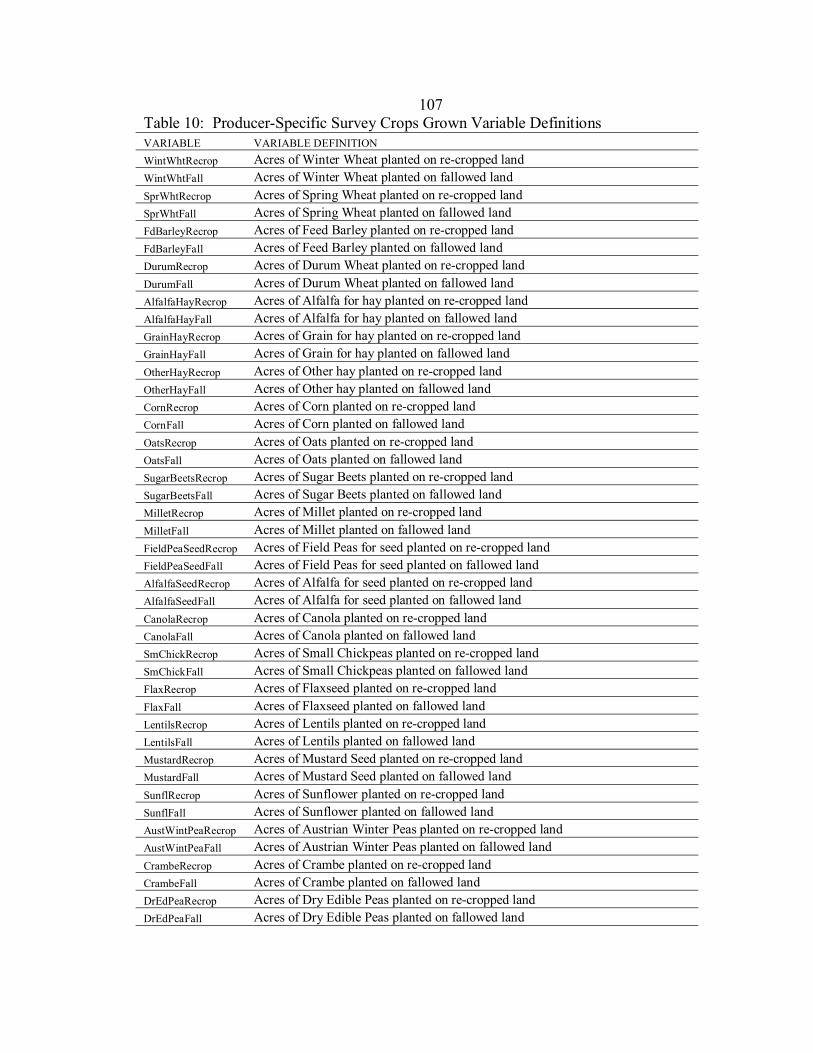
107

Table 10: Producer-Specific Survey Crops Grown Variable Definitions VARIABLE VARIABLE DEFINITION WintWhtRecrop Acres of Winter Wheat planted on re-cropped land WintWhtFall Acres of Winter Wheat planted on fallowed land SprWhtRecrop Acres of Spring Wheat planted on re-cropped land SprWhtFall Acres of Spring Wheat planted on fallowed land FdBarleyRecrop Acres of Feed Barley planted on re-cropped land FdBarleyFall Acres of Feed Barley planted on fallowed land DurumRecrop Acres of Durum Wheat planted on re-cropped land DurumFall Acres of Durum Wheat planted on fallowed land AlfalfaHayRecrop Acres of Alfalfa for hay planted on re-cropped land AlfalfaHayFall Acres of Alfalfa for hay planted on fallowed land GrainHayRecrop Acres of Grain for hay planted on re-cropped land GrainHayFall Acres of Grain for hay planted on fallowed land OtherHayRecrop Acres of Other hay planted on re-cropped land OtherHayFall Acres of Other hay planted on fallowed land CornRecrop Acres of Corn planted on re-cropped land CornFall Acres of Corn planted on fallowed land OatsRecrop Acres of Oats planted on re-cropped land OatsFall Acres of Oats planted on fallowed land SugarBeetsRecrop Acres of Sugar Beets planted on re-cropped land SugarBeetsFall Acres of Sugar Beets planted on fallowed land MilletRecrop Acres of Millet planted on re-cropped land MilletFall Acres of Millet planted on fallowed land FieldPeaSeedRecrop Acres of Field Peas for seed planted on re-cropped land FieldPeaSeedFall Acres of Field Peas for seed planted on fallowed land AlfalfaSeedRecrop Acres of Alfalfa for seed planted on re-cropped land AlfalfaSeedFall Acres of Alfalfa for seed planted on fallowed land CanolaRecrop Acres of Canola planted on re-cropped land CanolaFall Acres of Canola planted on fallowed land SmChickRecrop Acres of Small Chickpeas planted on re-cropped land SmChickFall Acres of Small Chickpeas planted on fallowed land FlaxRecrop Acres of Flaxseed planted on re-cropped land FlaxFall Acres of Flaxseed planted on fallowed land LentilsRecrop Acres of Lentils planted on re-cropped land LentilsFall Acres of Lentils planted on fallowed land MustardRecrop Acres of Mustard Seed planted on re-cropped land MustardFall Acres of Mustard Seed planted on fallowed land SunflRecrop Acres of Sunflower planted on re-cropped land SunflFall Acres of Sunflower planted on fallowed land AustWintPeaRecrop Acres of Austrian Winter Peas planted on re-cropped land AustWintPeaFall Acres of Austrian Winter Peas planted on fallowed land CrambeRecrop Acres of Crambe planted on re-cropped land CrambeFall Acres of Crambe planted on fallowed land DrEdPeaRecrop Acres of Dry Edible Peas planted on re-cropped land DrEdPeaFall Acres of Dry Edible Peas planted on fallowed land

108

Table 10: Producer-Specific Survey Crops Grown Variable Definitions (Continued) VARIABLE VARIABLE DEFINITION LgChickRecrop Acres of Large Chickpeas planted on re-cropped land LgChickFall Acres of Large Chickpeas planted on fallowed land MaltBarlRecrop Acres of Malting Barley planted on re-cropped land MaltBarlFall Acres of Malting Barley planted on fallowed land PintoBeanRecrop Acres of Pinto Beans planted on re-cropped land PintoBeanFall Acres of Pinto Beans planted on fallowed land SafflowerRecrop Acres of Safflower planted on re-cropped land SafflowerFall Acres of Safflower planted on fallowed land GrassSdRecrop Acres of Grass Seed planted on re-cropped land GrassSdFall Acres of Grass Seed planted on fallowed land CRP Acres of farming operation in the Conservation Reserve Program (CRP) Fallowed Acres of farming operation fallowed Crop Acreage Total acreage of farming operation Table 11: Producer-Specific Survey General Information Variable Definitions

VARIABLE VARIABLE DEFINITION Chouteau (0,1) Dummy for Chouteau as the county where farming operation is located Daniels (0,1) Dummy for Daniels as the county where farming operation is located McCone (0,1) Dummy for McCone as the county where farming operation is located Richland (0,1) Dummy for Richland as the county where farming operation is located Roosevelt (0,1) Dummy for Roosevelt as the county where farming operation is located Sheridan (0,1) Dummy for Sheridan as the county where farming operation is located Valley (0,1) Dummy for Valley as the county where farming operation is located Yellowstone (0,1) Dummy for Yellowstone as the county where farming operation is located

Northcentral (0,1) Dummy for Northcentral as the geographic region where farming operation is located

Northeast (0,1) Dummy for Northeast as the geographic region where farming operation is located

Southcentral (0,1) Dummy for Southcentral as the geographic region where farming operation is located

Years Farming Years of farming experience for farm operator Age Age of farm operator Some High School (0,1) Dummy for Some High School as highest educational level attained High School Diploma (0,1) Dummy for High School Diplomaas highest educational level attained Trade School (0,1) Dummy for Trade School as highest educational level attained Associate Degree (0,1) Dummy for Associates Degree as highest educational level attained Some College (0,1) Dummy for Some College as highest educational level attained College Degree (0,1) Dummy for College Degree as highest educational level attained Graduate Degree (0,1) Dummy for Graduate Degree as highest educational level attained College Graduate (0,1) Dummy combining College Degree and Graduate Degree Any College (0,1) Dummy combining Some College, College Degree, and Graduate Degree Computer (0,1) Dummy for ownership of a computer Bookkeeping on Computer (0,1) Dummy for performing of bookkeeping on a computer

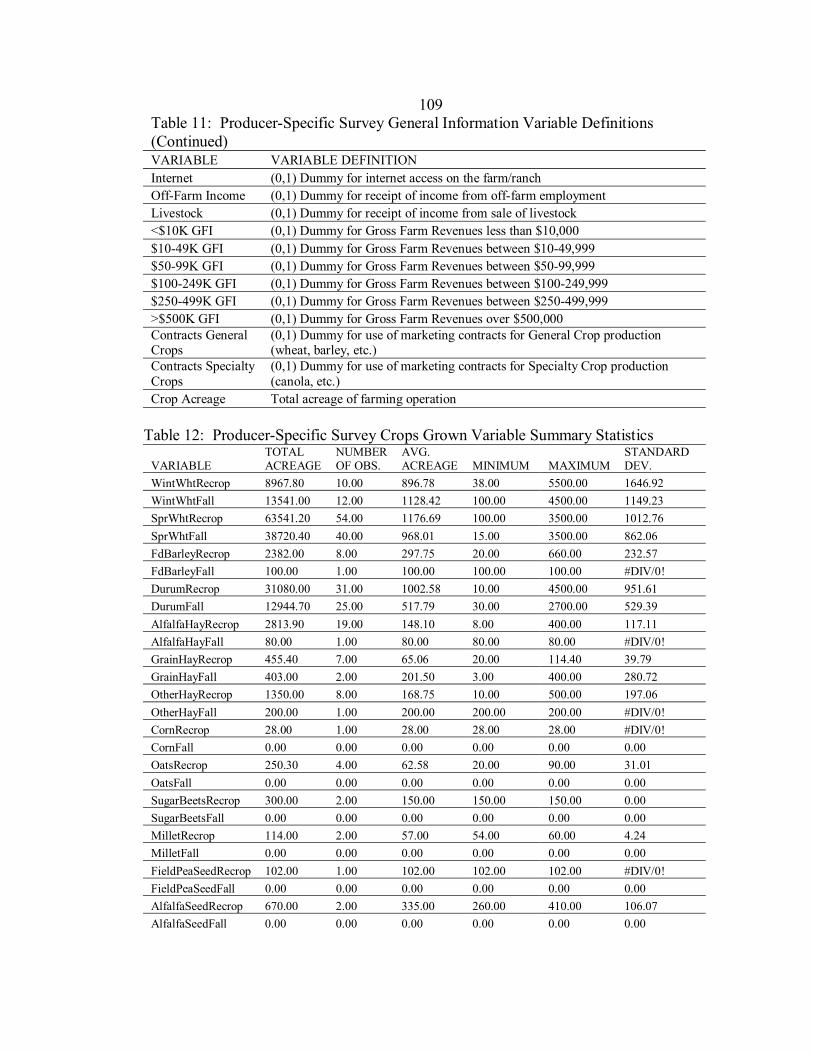
109

Table 11: Producer-Specific Survey General Information Variable Definitions (Continued) VARIABLE VARIABLE DEFINITION Internet (0,1) Dummy for internet access on the farm/ranch Off-Farm Income (0,1) Dummy for receipt of income from off-farm employment Livestock (0,1) Dummy for receipt of income from sale of livestock <$10K GFI (0,1) Dummy for Gross Farm Revenues less than $10,000 $10-49K GFI (0,1) Dummy for Gross Farm Revenues between $10-49,999 $50-99K GFI (0,1) Dummy for Gross Farm Revenues between $50-99,999 $100-249K GFI (0,1) Dummy for Gross Farm Revenues between $100-249,999 $250-499K GFI (0,1) Dummy for Gross Farm Revenues between $250-499,999 >$500K GFI (0,1) Dummy for Gross Farm Revenues over $500,000 Contracts General Crops

(0,1) Dummy for use of marketing contracts for General Crop production (wheat, barley, etc.)

Contracts Specialty Crops

(0,1) Dummy for use of marketing contracts for Specialty Crop production (canola, etc.)

Crop Acreage Total acreage of farming operation Table 12: Producer-Specific Survey Crops Grown Variable Summary Statistics

VARIABLE TOTAL ACREAGE

NUMBER OF OBS.

AVG. ACREAGE MINIMUM MAXIMUM

STANDARD DEV.

WintWhtRecrop 8967.80 10.00 896.78 38.00 5500.00 1646.92 WintWhtFall 13541.00 12.00 1128.42 100.00 4500.00 1149.23 SprWhtRecrop 63541.20 54.00 1176.69 100.00 3500.00 1012.76 SprWhtFall 38720.40 40.00 968.01 15.00 3500.00 862.06 FdBarleyRecrop 2382.00 8.00 297.75 20.00 660.00 232.57 FdBarleyFall 100.00 1.00 100.00 100.00 100.00 #DIV/0! DurumRecrop 31080.00 31.00 1002.58 10.00 4500.00 951.61 DurumFall 12944.70 25.00 517.79 30.00 2700.00 529.39 AlfalfaHayRecrop 2813.90 19.00 148.10 8.00 400.00 117.11 AlfalfaHayFall 80.00 1.00 80.00 80.00 80.00 #DIV/0! GrainHayRecrop 455.40 7.00 65.06 20.00 114.40 39.79 GrainHayFall 403.00 2.00 201.50 3.00 400.00 280.72 OtherHayRecrop 1350.00 8.00 168.75 10.00 500.00 197.06 OtherHayFall 200.00 1.00 200.00 200.00 200.00 #DIV/0! CornRecrop 28.00 1.00 28.00 28.00 28.00 #DIV/0! CornFall 0.00 0.00 0.00 0.00 0.00 0.00 OatsRecrop 250.30 4.00 62.58 20.00 90.00 31.01 OatsFall 0.00 0.00 0.00 0.00 0.00 0.00 SugarBeetsRecrop 300.00 2.00 150.00 150.00 150.00 0.00 SugarBeetsFall 0.00 0.00 0.00 0.00 0.00 0.00 MilletRecrop 114.00 2.00 57.00 54.00 60.00 4.24 MilletFall 0.00 0.00 0.00 0.00 0.00 0.00 FieldPeaSeedRecrop 102.00 1.00 102.00 102.00 102.00 #DIV/0! FieldPeaSeedFall 0.00 0.00 0.00 0.00 0.00 0.00 AlfalfaSeedRecrop 670.00 2.00 335.00 260.00 410.00 106.07 AlfalfaSeedFall 0.00 0.00 0.00 0.00 0.00 0.00

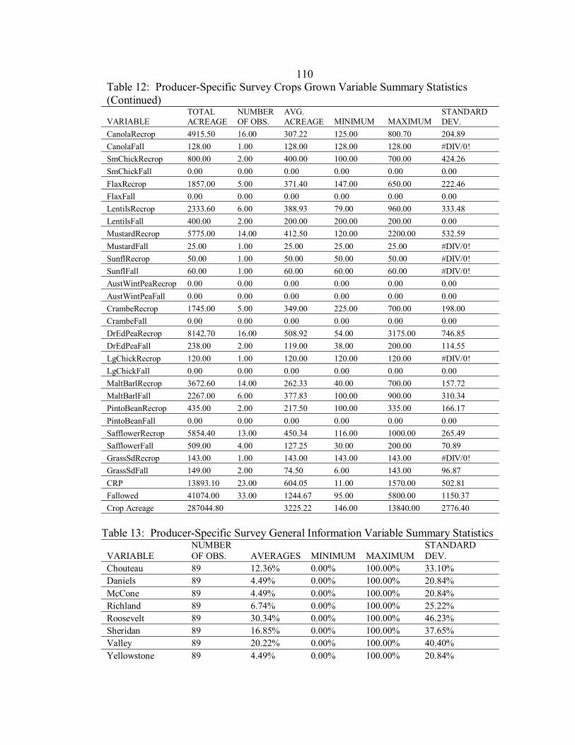
110

Table 12: Producer-Specific Survey Crops Grown Variable Summary Statistics (Continued)

VARIABLE TOTAL ACREAGE

NUMBER OF OBS.

AVG. ACREAGE MINIMUM MAXIMUM

STANDARD DEV.

CanolaRecrop 4915.50 16.00 307.22 125.00 800.70 204.89 CanolaFall 128.00 1.00 128.00 128.00 128.00 #DIV/0! SmChickRecrop 800.00 2.00 400.00 100.00 700.00 424.26 SmChickFall 0.00 0.00 0.00 0.00 0.00 0.00 FlaxRecrop 1857.00 5.00 371.40 147.00 650.00 222.46 FlaxFall 0.00 0.00 0.00 0.00 0.00 0.00 LentilsRecrop 2333.60 6.00 388.93 79.00 960.00 333.48 LentilsFall 400.00 2.00 200.00 200.00 200.00 0.00 MustardRecrop 5775.00 14.00 412.50 120.00 2200.00 532.59 MustardFall 25.00 1.00 25.00 25.00 25.00 #DIV/0! SunflRecrop 50.00 1.00 50.00 50.00 50.00 #DIV/0! SunflFall 60.00 1.00 60.00 60.00 60.00 #DIV/0! AustWintPeaRecrop 0.00 0.00 0.00 0.00 0.00 0.00 AustWintPeaFall 0.00 0.00 0.00 0.00 0.00 0.00 CrambeRecrop 1745.00 5.00 349.00 225.00 700.00 198.00 CrambeFall 0.00 0.00 0.00 0.00 0.00 0.00 DrEdPeaRecrop 8142.70 16.00 508.92 54.00 3175.00 746.85 DrEdPeaFall 238.00 2.00 119.00 38.00 200.00 114.55 LgChickRecrop 120.00 1.00 120.00 120.00 120.00 #DIV/0! LgChickFall 0.00 0.00 0.00 0.00 0.00 0.00 MaltBarlRecrop 3672.60 14.00 262.33 40.00 700.00 157.72 MaltBarlFall 2267.00 6.00 377.83 100.00 900.00 310.34 PintoBeanRecrop 435.00 2.00 217.50 100.00 335.00 166.17 PintoBeanFall 0.00 0.00 0.00 0.00 0.00 0.00 SafflowerRecrop 5854.40 13.00 450.34 116.00 1000.00 265.49 SafflowerFall 509.00 4.00 127.25 30.00 200.00 70.89 GrassSdRecrop 143.00 1.00 143.00 143.00 143.00 #DIV/0! GrassSdFall 149.00 2.00 74.50 6.00 143.00 96.87 CRP 13893.10 23.00 604.05 11.00 1570.00 502.81 Fallowed 41074.00 33.00 1244.67 95.00 5800.00 1150.37 Crop Acreage 287044.80 3225.22 146.00 13840.00 2776.40

Table 13: Producer-Specific Survey General Information Variable Summary Statistics

VARIABLE NUMBER OF OBS. AVERAGES MINIMUM MAXIMUM

STANDARD DEV.

Chouteau 89 12.36% 0.00% 100.00% 33.10% Daniels 89 4.49% 0.00% 100.00% 20.84% McCone 89 4.49% 0.00% 100.00% 20.84% Richland 89 6.74% 0.00% 100.00% 25.22% Roosevelt 89 30.34% 0.00% 100.00% 46.23% Sheridan 89 16.85% 0.00% 100.00% 37.65% Valley 89 20.22% 0.00% 100.00% 40.40% Yellowstone 89 4.49% 0.00% 100.00% 20.84%

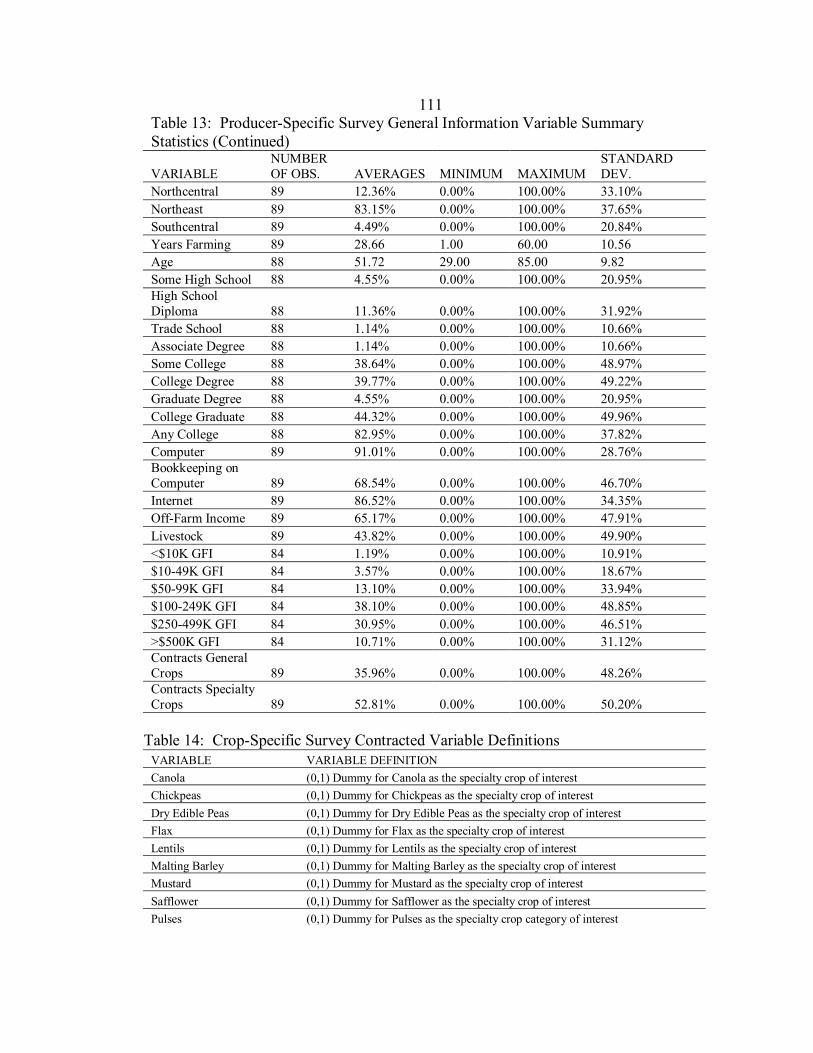
111

Table 13: Producer-Specific Survey General Information Variable Summary Statistics (Continued)

VARIABLE NUMBER OF OBS. AVERAGES MINIMUM MAXIMUM

STANDARD DEV.

Northcentral 89 12.36% 0.00% 100.00% 33.10% Northeast 89 83.15% 0.00% 100.00% 37.65% Southcentral 89 4.49% 0.00% 100.00% 20.84% Years Farming 89 28.66 1.00 60.00 10.56 Age 88 51.72 29.00 85.00 9.82 Some High School 88 4.55% 0.00% 100.00% 20.95% High School Diploma 88 11.36% 0.00% 100.00% 31.92% Trade School 88 1.14% 0.00% 100.00% 10.66% Associate Degree 88 1.14% 0.00% 100.00% 10.66% Some College 88 38.64% 0.00% 100.00% 48.97% College Degree 88 39.77% 0.00% 100.00% 49.22% Graduate Degree 88 4.55% 0.00% 100.00% 20.95% College Graduate 88 44.32% 0.00% 100.00% 49.96% Any College 88 82.95% 0.00% 100.00% 37.82% Computer 89 91.01% 0.00% 100.00% 28.76% Bookkeeping on Computer 89 68.54% 0.00% 100.00% 46.70% Internet 89 86.52% 0.00% 100.00% 34.35% Off-Farm Income 89 65.17% 0.00% 100.00% 47.91% Livestock 89 43.82% 0.00% 100.00% 49.90% <$10K GFI 84 1.19% 0.00% 100.00% 10.91% $10-49K GFI 84 3.57% 0.00% 100.00% 18.67% $50-99K GFI 84 13.10% 0.00% 100.00% 33.94% $100-249K GFI 84 38.10% 0.00% 100.00% 48.85% $250-499K GFI 84 30.95% 0.00% 100.00% 46.51% >$500K GFI 84 10.71% 0.00% 100.00% 31.12% Contracts General Crops 89 35.96% 0.00% 100.00% 48.26% Contracts Specialty Crops 89 52.81% 0.00% 100.00% 50.20%

Table 14: Crop-Specific Survey Contracted Variable Definitions

VARIABLE VARIABLE DEFINITION Canola (0,1) Dummy for Canola as the specialty crop of interest Chickpeas (0,1) Dummy for Chickpeas as the specialty crop of interest Dry Edible Peas (0,1) Dummy for Dry Edible Peas as the specialty crop of interest Flax (0,1) Dummy for Flax as the specialty crop of interest Lentils (0,1) Dummy for Lentils as the specialty crop of interest Malting Barley (0,1) Dummy for Malting Barley as the specialty crop of interest Mustard (0,1) Dummy for Mustard as the specialty crop of interest Safflower (0,1) Dummy for Safflower as the specialty crop of interest Pulses (0,1) Dummy for Pulses as the specialty crop category of interest

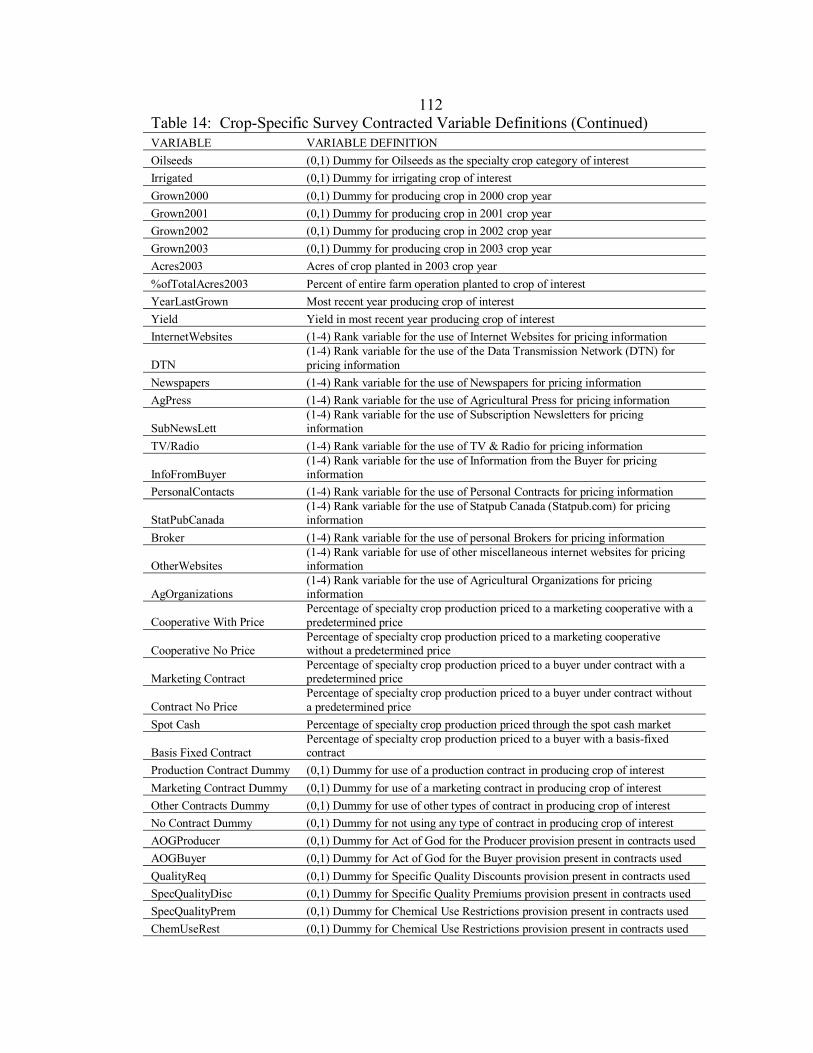
112

Table 14: Crop-Specific Survey Contracted Variable Definitions (Continued) VARIABLE VARIABLE DEFINITION Oilseeds (0,1) Dummy for Oilseeds as the specialty crop category of interest Irrigated (0,1) Dummy for irrigating crop of interest Grown2000 (0,1) Dummy for producing crop in 2000 crop year Grown2001 (0,1) Dummy for producing crop in 2001 crop year Grown2002 (0,1) Dummy for producing crop in 2002 crop year Grown2003 (0,1) Dummy for producing crop in 2003 crop year Acres2003 Acres of crop planted in 2003 crop year %ofTotalAcres2003 Percent of entire farm operation planted to crop of interest YearLastGrown Most recent year producing crop of interest Yield Yield in most recent year producing crop of interest InternetWebsites (1-4) Rank variable for the use of Internet Websites for pricing information

DTN (1-4) Rank variable for the use of the Data Transmission Network (DTN) for pricing information

Newspapers (1-4) Rank variable for the use of Newspapers for pricing information AgPress (1-4) Rank variable for the use of Agricultural Press for pricing information

SubNewsLett (1-4) Rank variable for the use of Subscription Newsletters for pricing information

TV/Radio (1-4) Rank variable for the use of TV & Radio for pricing information

InfoFromBuyer (1-4) Rank variable for the use of Information from the Buyer for pricing information

PersonalContacts (1-4) Rank variable for the use of Personal Contracts for pricing information

StatPubCanada (1-4) Rank variable for the use of Statpub Canada (Statpub.com) for pricing information

Broker (1-4) Rank variable for the use of personal Brokers for pricing information

OtherWebsites (1-4) Rank variable for use of other miscellaneous internet websites for pricing information

AgOrganizations (1-4) Rank variable for the use of Agricultural Organizations for pricing information

Cooperative With Price Percentage of specialty crop production priced to a marketing cooperative with a predetermined price

Cooperative No Price Percentage of specialty crop production priced to a marketing cooperative without a predetermined price

Marketing Contract Percentage of specialty crop production priced to a buyer under contract with a predetermined price

Contract No Price Percentage of specialty crop production priced to a buyer under contract without a predetermined price

Spot Cash Percentage of specialty crop production priced through the spot cash market

Basis Fixed Contract Percentage of specialty crop production priced to a buyer with a basis-fixed contract

Production Contract Dummy (0,1) Dummy for use of a production contract in producing crop of interest Marketing Contract Dummy (0,1) Dummy for use of a marketing contract in producing crop of interest Other Contracts Dummy (0,1) Dummy for use of other types of contract in producing crop of interest No Contract Dummy (0,1) Dummy for not using any type of contract in producing crop of interest AOGProducer (0,1) Dummy for Act of God for the Producer provision present in contracts used AOGBuyer (0,1) Dummy for Act of God for the Buyer provision present in contracts used QualityReq (0,1) Dummy for Specific Quality Discounts provision present in contracts used SpecQualityDisc (0,1) Dummy for Specific Quality Premiums provision present in contracts used SpecQualityPrem (0,1) Dummy for Chemical Use Restrictions provision present in contracts used ChemUseRest (0,1) Dummy for Chemical Use Restrictions provision present in contracts used

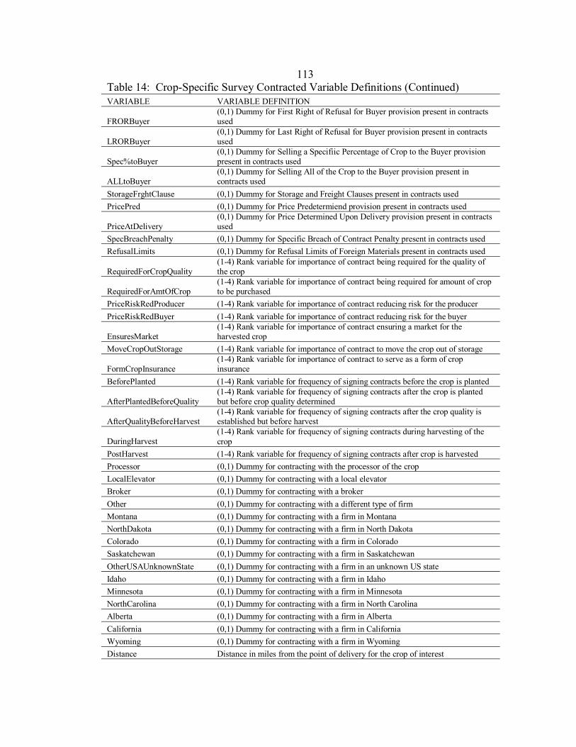
113

Table 14: Crop-Specific Survey Contracted Variable Definitions (Continued) VARIABLE VARIABLE DEFINITION

FRORBuyer (0,1) Dummy for First Right of Refusal for Buyer provision present in contracts used

LRORBuyer (0,1) Dummy for Last Right of Refusal for Buyer provision present in contracts used

Spec%toBuyer (0,1) Dummy for Selling a Specifiic Percentage of Crop to the Buyer provision present in contracts used

ALLtoBuyer (0,1) Dummy for Selling All of the Crop to the Buyer provision present in contracts used

StorageFrghtClause (0,1) Dummy for Storage and Freight Clauses present in contracts used PricePred (0,1) Dummy for Price Predetermiend provision present in contracts used

PriceAtDelivery (0,1) Dummy for Price Determined Upon Delivery provision present in contracts used

SpecBreachPenalty (0,1) Dummy for Specific Breach of Contract Penalty present in contracts used RefusalLimits (0,1) Dummy for Refusal Limits of Foreign Materials present in contracts used

RequiredForCropQuality (1-4) Rank variable for importance of contract being required for the quality of the crop

RequiredForAmtOfCrop (1-4) Rank variable for importance of contract being required for amount of crop to be purchased

PriceRiskRedProducer (1-4) Rank variable for importance of contract reducing risk for the producer PriceRiskRedBuyer (1-4) Rank variable for importance of contract reducing risk for the buyer

EnsuresMarket (1-4) Rank variable for importance of contract ensuring a market for the harvested crop

MoveCropOutStorage (1-4) Rank variable for importance of contract to move the crop out of storage

FormCropInsurance (1-4) Rank variable for importance of contract to serve as a form of crop insurance

BeforePlanted (1-4) Rank variable for frequency of signing contracts before the crop is planted

AfterPlantedBeforeQuality (1-4) Rank variable for frequency of signing contracts after the crop is planted but before crop quality determined

AfterQualityBeforeHarvest (1-4) Rank variable for frequency of signing contracts after the crop quality is established but before harvest

DuringHarvest (1-4) Rank variable for frequency of signing contracts during harvesting of the crop

PostHarvest (1-4) Rank variable for frequency of signing contracts after crop is harvested Processor (0,1) Dummy for contracting with the processor of the crop LocalElevator (0,1) Dummy for contracting with a local elevator Broker (0,1) Dummy for contracting with a broker Other (0,1) Dummy for contracting with a different type of firm Montana (0,1) Dummy for contracting with a firm in Montana NorthDakota (0,1) Dummy for contracting with a firm in North Dakota Colorado (0,1) Dummy for contracting with a firm in Colorado Saskatchewan (0,1) Dummy for contracting with a firm in Saskatchewan OtherUSAUnknownState (0,1) Dummy for contracting with a firm in an unknown US state Idaho (0,1) Dummy for contracting with a firm in Idaho Minnesota (0,1) Dummy for contracting with a firm in Minnesota NorthCarolina (0,1) Dummy for contracting with a firm in North Carolina Alberta (0,1) Dummy for contracting with a firm in Alberta California (0,1) Dummy for contracting with a firm in California Wyoming (0,1) Dummy for contracting with a firm in Wyoming Distance Distance in miles from the point of delivery for the crop of interest

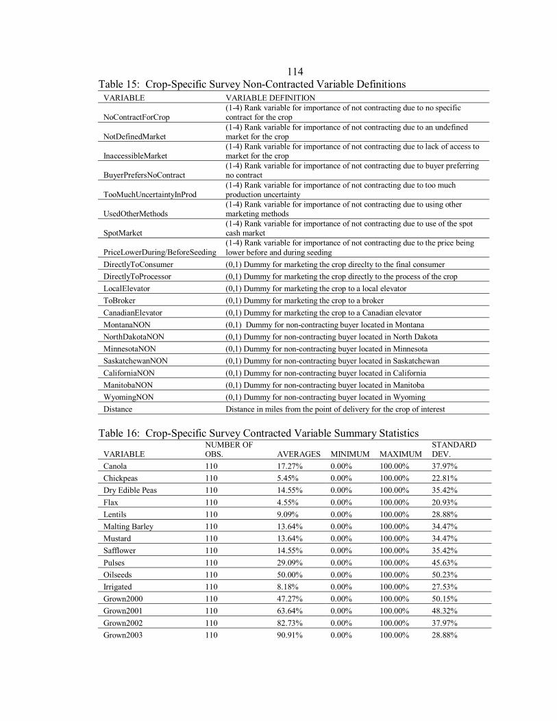
114

Table 15: Crop-Specific Survey Non-Contracted Variable Definitions VARIABLE VARIABLE DEFINITION

NoContractForCrop (1-4) Rank variable for importance of not contracting due to no specific contract for the crop

NotDefinedMarket (1-4) Rank variable for importance of not contracting due to an undefined market for the crop

InaccessibleMarket (1-4) Rank variable for importance of not contracting due to lack of access to market for the crop

BuyerPrefersNoContract (1-4) Rank variable for importance of not contracting due to buyer preferring no contract

TooMuchUncertaintyInProd (1-4) Rank variable for importance of not contracting due to too much production uncertainty

UsedOtherMethods (1-4) Rank variable for importance of not contracting due to using other marketing methods

SpotMarket (1-4) Rank variable for importance of not contracting due to use of the spot cash market

PriceLowerDuring/BeforeSeeding (1-4) Rank variable for importance of not contracting due to the price being lower before and during seeding

DirectlyToConsumer (0,1) Dummy for marketing the crop direclty to the final consumer DirectlyToProcessor (0,1) Dummy for marketing the crop directly to the process of the crop LocalElevator (0,1) Dummy for marketing the crop to a local elevator ToBroker (0,1) Dummy for marketing the crop to a broker CanadianElevator (0,1) Dummy for marketing the crop to a Canadian elevator MontanaNON (0,1) Dummy for non-contracting buyer located in Montana NorthDakotaNON (0,1) Dummy for non-contracting buyer located in North Dakota MinnesotaNON (0,1) Dummy for non-contracting buyer located in Minnesota SaskatchewanNON (0,1) Dummy for non-contracting buyer located in Saskatchewan CaliforniaNON (0,1) Dummy for non-contracting buyer located in California ManitobaNON (0,1) Dummy for non-contracting buyer located in Manitoba WyomingNON (0,1) Dummy for non-contracting buyer located in Wyoming Distance Distance in miles from the point of delivery for the crop of interest

Table 16: Crop-Specific Survey Contracted Variable Summary Statistics

VARIABLE NUMBER OF OBS. AVERAGES MINIMUM MAXIMUM

STANDARD DEV.

Canola 110 17.27% 0.00% 100.00% 37.97% Chickpeas 110 5.45% 0.00% 100.00% 22.81% Dry Edible Peas 110 14.55% 0.00% 100.00% 35.42% Flax 110 4.55% 0.00% 100.00% 20.93% Lentils 110 9.09% 0.00% 100.00% 28.88% Malting Barley 110 13.64% 0.00% 100.00% 34.47% Mustard 110 13.64% 0.00% 100.00% 34.47% Safflower 110 14.55% 0.00% 100.00% 35.42% Pulses 110 29.09% 0.00% 100.00% 45.63% Oilseeds 110 50.00% 0.00% 100.00% 50.23% Irrigated 110 8.18% 0.00% 100.00% 27.53% Grown2000 110 47.27% 0.00% 100.00% 50.15% Grown2001 110 63.64% 0.00% 100.00% 48.32% Grown2002 110 82.73% 0.00% 100.00% 37.97% Grown2003 110 90.91% 0.00% 100.00% 28.88%

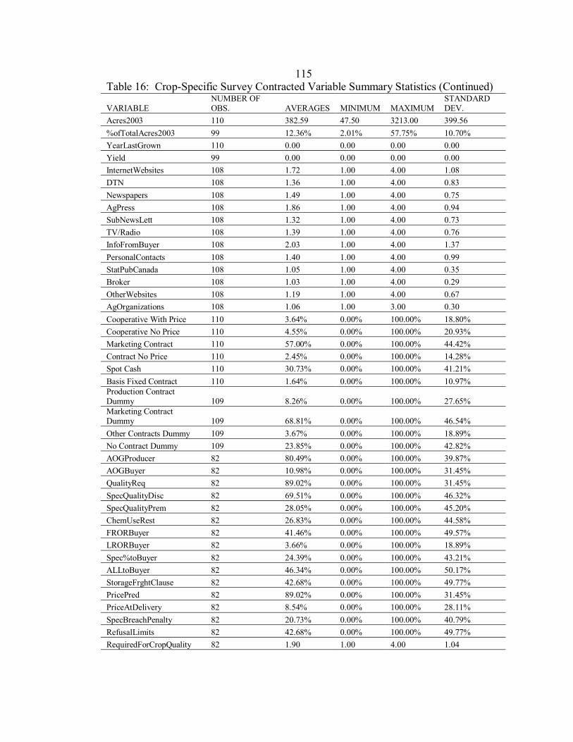
115

Table 16: Crop-Specific Survey Contracted Variable Summary Statistics (Continued)

VARIABLE NUMBER OF OBS. AVERAGES MINIMUM MAXIMUM

STANDARD DEV.

Acres2003 110 382.59 47.50 3213.00 399.56 %ofTotalAcres2003 99 12.36% 2.01% 57.75% 10.70% YearLastGrown 110 0.00 0.00 0.00 0.00 Yield 99 0.00 0.00 0.00 0.00 InternetWebsites 108 1.72 1.00 4.00 1.08 DTN 108 1.36 1.00 4.00 0.83 Newspapers 108 1.49 1.00 4.00 0.75 AgPress 108 1.86 1.00 4.00 0.94 SubNewsLett 108 1.32 1.00 4.00 0.73 TV/Radio 108 1.39 1.00 4.00 0.76 InfoFromBuyer 108 2.03 1.00 4.00 1.37 PersonalContacts 108 1.40 1.00 4.00 0.99 StatPubCanada 108 1.05 1.00 4.00 0.35 Broker 108 1.03 1.00 4.00 0.29 OtherWebsites 108 1.19 1.00 4.00 0.67 AgOrganizations 108 1.06 1.00 3.00 0.30 Cooperative With Price 110 3.64% 0.00% 100.00% 18.80% Cooperative No Price 110 4.55% 0.00% 100.00% 20.93% Marketing Contract 110 57.00% 0.00% 100.00% 44.42% Contract No Price 110 2.45% 0.00% 100.00% 14.28% Spot Cash 110 30.73% 0.00% 100.00% 41.21% Basis Fixed Contract 110 1.64% 0.00% 100.00% 10.97% Production Contract Dummy 109 8.26% 0.00% 100.00% 27.65% Marketing Contract Dummy 109 68.81% 0.00% 100.00% 46.54% Other Contracts Dummy 109 3.67% 0.00% 100.00% 18.89% No Contract Dummy 109 23.85% 0.00% 100.00% 42.82% AOGProducer 82 80.49% 0.00% 100.00% 39.87% AOGBuyer 82 10.98% 0.00% 100.00% 31.45% QualityReq 82 89.02% 0.00% 100.00% 31.45% SpecQualityDisc 82 69.51% 0.00% 100.00% 46.32% SpecQualityPrem 82 28.05% 0.00% 100.00% 45.20% ChemUseRest 82 26.83% 0.00% 100.00% 44.58% FRORBuyer 82 41.46% 0.00% 100.00% 49.57% LRORBuyer 82 3.66% 0.00% 100.00% 18.89% Spec%toBuyer 82 24.39% 0.00% 100.00% 43.21% ALLtoBuyer 82 46.34% 0.00% 100.00% 50.17% StorageFrghtClause 82 42.68% 0.00% 100.00% 49.77% PricePred 82 89.02% 0.00% 100.00% 31.45% PriceAtDelivery 82 8.54% 0.00% 100.00% 28.11% SpecBreachPenalty 82 20.73% 0.00% 100.00% 40.79% RefusalLimits 82 42.68% 0.00% 100.00% 49.77% RequiredForCropQuality 82 1.90 1.00 4.00 1.04

116

Table 16: Crop-Specific Survey Contracted Variable Summary Statistics (Continued)

VARIABLE NUMBER OF OBS. AVERAGES MINIMUM MAXIMUM

STANDARD DEV.

RequiredForAmtOfCrop 82 2.52 1.00 4.00 1.22 PriceRiskRedProducer 82 3.33 1.00 4.00 0.93 PriceRiskRedBuyer 82 1.46 1.00 4.00 0.83 EnsuresMarket 82 3.30 1.00 4.00 0.90 MoveCropOutStorage 82 1.04 1.00 4.00 0.33 FormCropInsurance 82 1.04 1.00 4.00 0.33 BeforePlanted 80 3.39 1.00 4.00 1.08 AfterPlantedBeforeQuality 80 1.45 1.00 4.00 0.71 AfterQualityBeforeHarvest 80 1.40 1.00 4.00 0.69 DuringHarvest 80 1.38 1.00 4.00 0.66 PostHarvest 80 1.96 1.00 4.00 1.20 Processor 83 83.13% 0.00% 100.00% 37.67% LocalElevator 83 28.92% 0.00% 100.00% 45.61% Broker 83 34.94% 0.00% 100.00% 47.97% Other 83 0.00% 0.00% 0.00% 0.00% Montana 83 48.19% 0.00% 100.00% 50.27% North Dakota 83 21.69% 0.00% 100.00% 41.46% Colorado 83 3.61% 0.00% 100.00% 18.78% Saskatchewan 83 33.73% 0.00% 100.00% 47.57% Other USA Unknown State 83 2.41% 0.00% 100.00% 15.43% Idaho 83 4.82% 0.00% 100.00% 21.55% Minnesota 83 2.41% 0.00% 100.00% 15.43% North Carolina 83 3.61% 0.00% 100.00% 18.78% Alberta 83 6.02% 0.00% 100.00% 23.94% California 83 8.43% 0.00% 100.00% 27.96% Wyoming 83 1.20% 0.00% 100.00% 10.98% Distance 81 78.80 0.00 500.00 94.10

Table 17: Crop-Specific Survey Non-Contracted Variable Summary Statistics

VARIABLE NUMBER OF OBS. AVERAGES MINIMUM MAXIMUM

STANDARD DEV.

NoContractForCrop 42 1.98 1.00 4.00 1.26 NotDefinedMarket 42 1.36 1.00 4.00 0.82 InaccessibleMarket 42 1.38 1.00 4.00 0.73 BuyerPrefersNoContract 42 1.33 1.00 4.00 0.75 TooMuchUncertaintyInProd 42 2.43 1.00 4.00 1.33 UsedOtherMethods 42 1.29 1.00 4.00 0.81 SpotMarket 42 1.00 1.00 1.00 0.00 PriceLowerDuring/BeforeSeeding 42 1.10 1.00 3.00 0.43 DirectlyToConsumer 45 2.22% 0.00% 100.00% 14.91% DirectlyToProcessor 45 53.33% 0.00% 100.00% 50.45% LocalElevator 45 35.56% 0.00% 100.00% 48.41% ToBroker 45 31.11% 0.00% 100.00% 46.82% CanadianElevator 45 4.44% 0.00% 100.00% 20.84%

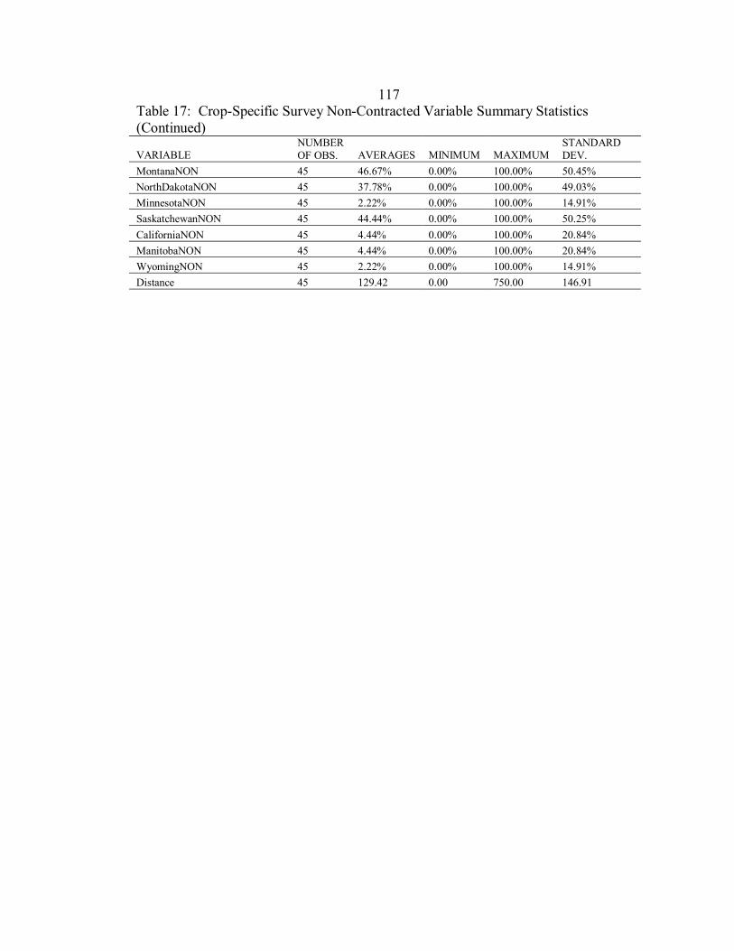
117

Table 17: Crop-Specific Survey Non-Contracted Variable Summary Statistics (Continued)

VARIABLE NUMBER OF OBS. AVERAGES MINIMUM MAXIMUM

STANDARD DEV.

MontanaNON 45 46.67% 0.00% 100.00% 50.45% NorthDakotaNON 45 37.78% 0.00% 100.00% 49.03% MinnesotaNON 45 2.22% 0.00% 100.00% 14.91% SaskatchewanNON 45 44.44% 0.00% 100.00% 50.25% CaliforniaNON 45 4.44% 0.00% 100.00% 20.84% ManitobaNON 45 4.44% 0.00% 100.00% 20.84% WyomingNON 45 2.22% 0.00% 100.00% 14.91% Distance 45 129.42 0.00 750.00 146.91

118

APPENDIX D

VARIANCE/COVARIANCE CORRELATION MATRICES

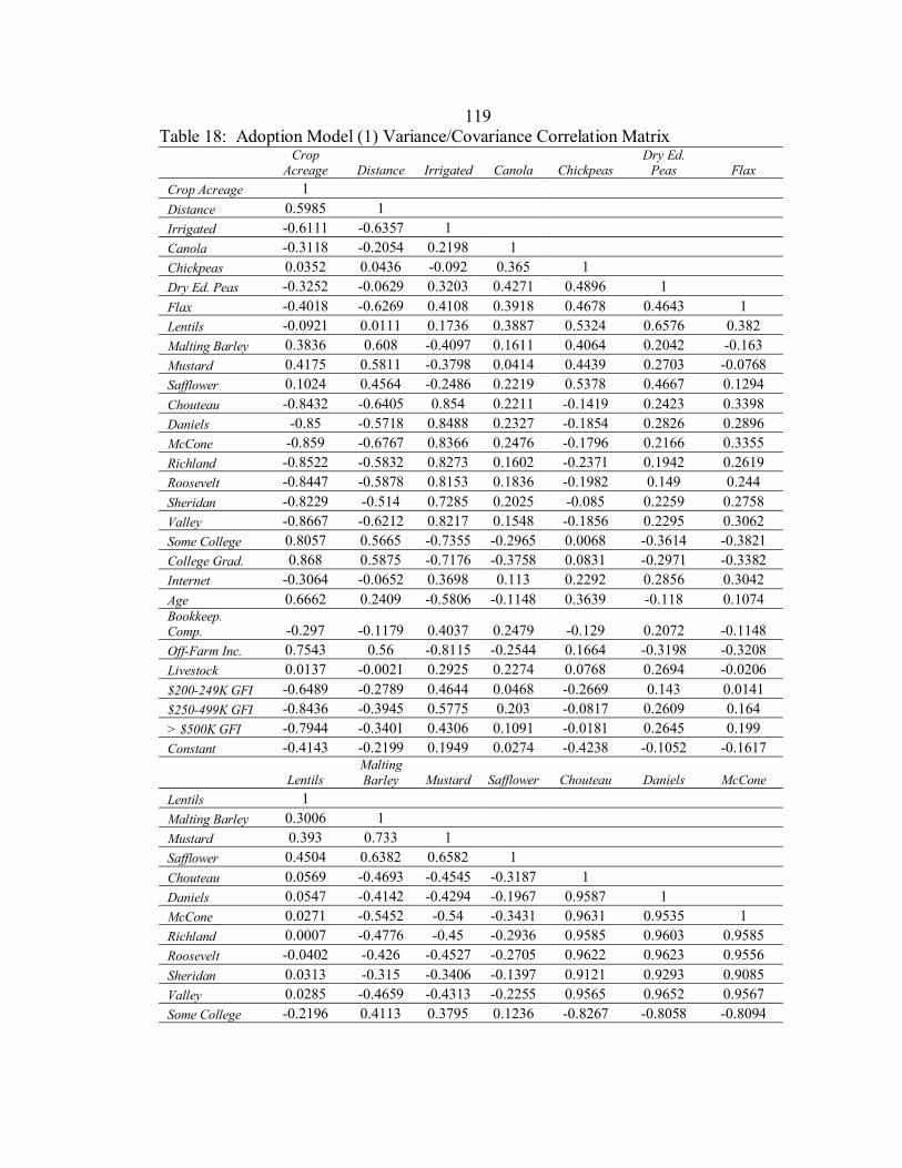
119

Table 18: Adoption Model (1) Variance/Covariance Correlation Matrix

Crop

Acreage Distance Irrigated Canola Chickpeas Dry Ed.

Peas Flax Crop Acreage 1 Distance 0.5985 1 Irrigated -0.6111 -0.6357 1 Canola -0.3118 -0.2054 0.2198 1 Chickpeas 0.0352 0.0436 -0.092 0.365 1 Dry Ed. Peas -0.3252 -0.0629 0.3203 0.4271 0.4896 1 Flax -0.4018 -0.6269 0.4108 0.3918 0.4678 0.4643 1 Lentils -0.0921 0.0111 0.1736 0.3887 0.5324 0.6576 0.382 Malting Barley 0.3836 0.608 -0.4097 0.1611 0.4064 0.2042 -0.163 Mustard 0.4175 0.5811 -0.3798 0.0414 0.4439 0.2703 -0.0768 Safflower 0.1024 0.4564 -0.2486 0.2219 0.5378 0.4667 0.1294 Chouteau -0.8432 -0.6405 0.854 0.2211 -0.1419 0.2423 0.3398 Daniels -0.85 -0.5718 0.8488 0.2327 -0.1854 0.2826 0.2896 McCone -0.859 -0.6767 0.8366 0.2476 -0.1796 0.2166 0.3355 Richland -0.8522 -0.5832 0.8273 0.1602 -0.2371 0.1942 0.2619 Roosevelt -0.8447 -0.5878 0.8153 0.1836 -0.1982 0.149 0.244 Sheridan -0.8229 -0.514 0.7285 0.2025 -0.085 0.2259 0.2758 Valley -0.8667 -0.6212 0.8217 0.1548 -0.1856 0.2295 0.3062 Some College 0.8057 0.5665 -0.7355 -0.2965 0.0068 -0.3614 -0.3821 College Grad. 0.868 0.5875 -0.7176 -0.3758 0.0831 -0.2971 -0.3382 Internet -0.3064 -0.0652 0.3698 0.113 0.2292 0.2856 0.3042 Age 0.6662 0.2409 -0.5806 -0.1148 0.3639 -0.118 0.1074 Bookkeep. Comp. -0.297 -0.1179 0.4037 0.2479 -0.129 0.2072 -0.1148 Off-Farm Inc. 0.7543 0.56 -0.8115 -0.2544 0.1664 -0.3198 -0.3208 Livestock 0.0137 -0.0021 0.2925 0.2274 0.0768 0.2694 -0.0206 $200-249K GFI -0.6489 -0.2789 0.4644 0.0468 -0.2669 0.143 0.0141 $250-499K GFI -0.8436 -0.3945 0.5775 0.203 -0.0817 0.2609 0.164 > $500K GFI -0.7944 -0.3401 0.4306 0.1091 -0.0181 0.2645 0.199 Constant -0.4143 -0.2199 0.1949 0.0274 -0.4238 -0.1052 -0.1617

Lentils Malting Barley Mustard Safflower Chouteau Daniels McCone

Lentils 1 Malting Barley 0.3006 1 Mustard 0.393 0.733 1 Safflower 0.4504 0.6382 0.6582 1 Chouteau 0.0569 -0.4693 -0.4545 -0.3187 1 Daniels 0.0547 -0.4142 -0.4294 -0.1967 0.9587 1 McCone 0.0271 -0.5452 -0.54 -0.3431 0.9631 0.9535 1 Richland 0.0007 -0.4776 -0.45 -0.2936 0.9585 0.9603 0.9585 Roosevelt -0.0402 -0.426 -0.4527 -0.2705 0.9622 0.9623 0.9556 Sheridan 0.0313 -0.315 -0.3406 -0.1397 0.9121 0.9293 0.9085 Valley 0.0285 -0.4659 -0.4313 -0.2255 0.9565 0.9652 0.9567 Some College -0.2196 0.4113 0.3795 0.1236 -0.8267 -0.8058 -0.8094

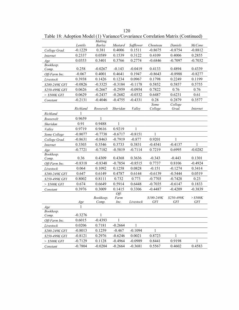
120

Table 18: Adoption Model (1) Variance/Covariance Correlation Matrix (Continued)

Lentils Malting Barley Mustard Safflower Chouteau Daniels McCone

College Grad. -0.1229 0.381 0.4006 0.1511 -0.8675 -0.8754 -0.8812 Internet 0.2337 0.0589 0.1539 0.3122 0.4109 0.4006 0.2855 Age 0.0353 0.3401 0.3766 0.2774 -0.6846 -0.7097 -0.7032 Bookkeep. Comp. 0.258 -0.0267 -0.143 -0.0419 0.4133 0.4894 0.4339 Off-Farm Inc. -0.067 0.4001 0.4641 0.1947 -0.8643 -0.8988 -0.8277 Livestock 0.3938 0.1426 0.1234 0.0967 0.1798 0.2249 0.1199 $200-249K GFI -0.0826 -0.3325 -0.3184 -0.1178 0.5852 0.5857 0.5755 $250-499K GFI 0.0626 -0.2667 -0.2959 -0.0954 0.7822 0.76 0.76 > $500K GFI 0.0629 -0.2437 -0.2682 -0.0332 0.6487 0.6231 0.61 Constant -0.2131 -0.4046 -0.4755 -0.4331 0.28 0.2879 0.3577

Richland Roosevelt Sheridan Valley Some

College College Grad. Internet

Richland 1 Roosevelt 0.9659 1 Sheridan 0.91 0.9488 1 Valley 0.9719 0.9616 0.9219 1 Some College -0.8077 -0.7738 -0.6717 -0.8151 1 College Grad. -0.8631 -0.8463 -0.7919 -0.877 0.9201 1 Internet 0.3303 0.3546 0.3733 0.3831 -0.4541 -0.4137 1 Age -0.7721 -0.7182 -0.5819 -0.7114 0.7219 0.6995 -0.0282 Bookkeep. Comp. 0.36 0.4309 0.4368 0.3636 -0.343 -0.443 0.1301 Off-Farm Inc. -0.8318 -0.8348 -0.7854 -0.8515 0.7737 0.8106 -0.4924 Livestock 0.064 0.1092 0.1258 0.0828 -0.151 -0.1274 0.3414 $200-249K GFI 0.647 0.6149 0.4787 0.6144 -0.6139 -0.5444 0.0519 $250-499K GFI 0.8002 0.8111 0.732 0.773 -0.7703 -0.7428 0.23 > $500K GFI 0.674 0.6649 0.5914 0.6448 -0.7035 -0.6147 0.1833 Constant 0.3976 0.3009 0.1415 0.3306 -0.4487 -0.4209 -0.3839

Age Bookkeep.

Comp.

Off-Farm Inc. Livestock

$100-249K GFI

$250-499K GFI

>$500K GFI

Age 1 Bookkeep. Comp. -0.3276 1 Off-Farm Inc. 0.6015 -0.4393 1 Livestock 0.0206 0.7181 -0.2664 1 $200-249K GFI -0.8013 0.1259 -0.467 -0.1094 1 $250-499K GFI -0.8121 0.2976 -0.6246 0.0021 0.8723 1 > $500K GFI -0.7129 0.1128 -0.4964 -0.0989 0.8441 0.9198 1 Constant -0.7804 -0.0204 -0.2664 -0.3681 0.5567 0.4602 0.4583

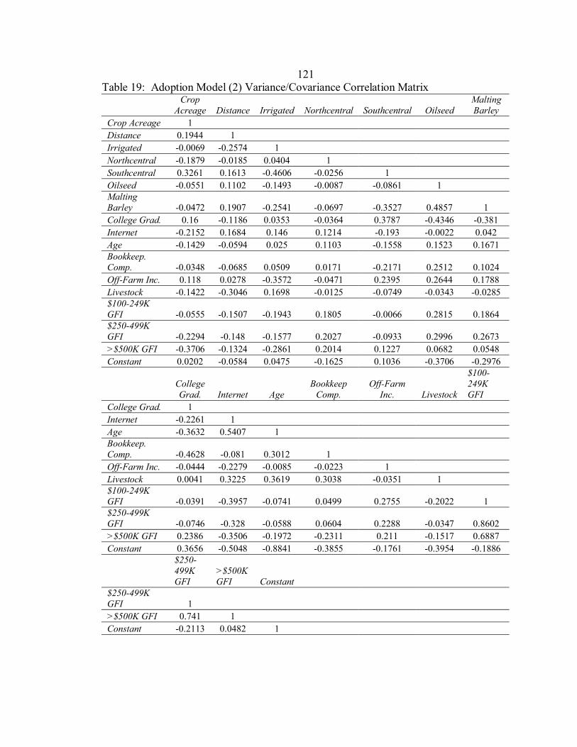
121

Table 19: Adoption Model (2) Variance/Covariance Correlation Matrix

Crop

Acreage Distance Irrigated Northcentral Southcentral Oilseed Malting Barley

Crop Acreage 1 Distance 0.1944 1 Irrigated -0.0069 -0.2574 1 Northcentral -0.1879 -0.0185 0.0404 1 Southcentral 0.3261 0.1613 -0.4606 -0.0256 1 Oilseed -0.0551 0.1102 -0.1493 -0.0087 -0.0861 1 Malting Barley -0.0472 0.1907 -0.2541 -0.0697 -0.3527 0.4857 1 College Grad. 0.16 -0.1186 0.0353 -0.0364 0.3787 -0.4346 -0.381 Internet -0.2152 0.1684 0.146 0.1214 -0.193 -0.0022 0.042 Age -0.1429 -0.0594 0.025 0.1103 -0.1558 0.1523 0.1671 Bookkeep. Comp. -0.0348 -0.0685 0.0509 0.0171 -0.2171 0.2512 0.1024 Off-Farm Inc. 0.118 0.0278 -0.3572 -0.0471 0.2395 0.2644 0.1788 Livestock -0.1422 -0.3046 0.1698 -0.0125 -0.0749 -0.0343 -0.0285 $100-249K GFI -0.0555 -0.1507 -0.1943 0.1805 -0.0066 0.2815 0.1864 $250-499K GFI -0.2294 -0.148 -0.1577 0.2027 -0.0933 0.2996 0.2673 >$500K GFI -0.3706 -0.1324 -0.2861 0.2014 0.1227 0.0682 0.0548 Constant 0.0202 -0.0584 0.0475 -0.1625 0.1036 -0.3706 -0.2976

College Grad. Internet Age

Bookkeep Comp.

Off-Farm Inc. Livestock

$100-249K GFI

College Grad. 1 Internet -0.2261 1 Age -0.3632 0.5407 1 Bookkeep. Comp. -0.4628 -0.081 0.3012 1 Off-Farm Inc. -0.0444 -0.2279 -0.0085 -0.0223 1 Livestock 0.0041 0.3225 0.3619 0.3038 -0.0351 1 $100-249K GFI -0.0391 -0.3957 -0.0741 0.0499 0.2755 -0.2022 1 $250-499K GFI -0.0746 -0.328 -0.0588 0.0604 0.2288 -0.0347 0.8602 >$500K GFI 0.2386 -0.3506 -0.1972 -0.2311 0.211 -0.1517 0.6887 Constant 0.3656 -0.5048 -0.8841 -0.3855 -0.1761 -0.3954 -0.1886

$250-499K GFI

>$500K GFI Constant

$250-499K GFI 1 >$500K GFI 0.741 1 Constant -0.2113 0.0482 1

122

Table 20: Adoption Model (3) Variance/Covariance Correlation Matrix

Crop

Acreage Distance Irrigated Northcentral Southcentral Oilseed Malting Barley

Crop Acreage 1 Distance 0.1944 1 Irrigated -0.0069 -0.2574 1 Northcentral -0.1879 -0.0185 0.0404 1 Southcentral 0.3261 0.1613 -0.4606 -0.0256 1 Oilseed -0.0551 0.1102 -0.1493 -0.0087 -0.0861 1 Malting Barley -0.0472 0.1907 -0.2541 -0.0697 -0.3527 0.4857 1 Any College 0.16 -0.1186 0.0353 -0.0364 0.3787 -0.4346 -0.381 Internet -0.2152 0.1684 0.146 0.1214 -0.193 -0.0022 0.042 Age -0.1429 -0.0594 0.025 0.1103 -0.1558 0.1523 0.1671 Bookkeep. Comp. -0.0348 -0.0685 0.0509 0.0171 -0.2171 0.2512 0.1024 Off-Farm Inc. 0.118 0.0278 -0.3572 -0.0471 0.2395 0.2644 0.1788 Livestock -0.1422 -0.3046 0.1698 -0.0125 -0.0749 -0.0343 -0.0285 $100-249K GFI -0.0555 -0.1507 -0.1943 0.1805 -0.0066 0.2815 0.1864 $250-499K GFI -0.2294 -0.148 -0.1577 0.2027 -0.0933 0.2996 0.2673 >$500K GFI -0.3706 -0.1324 -0.2861 0.2014 0.1227 0.0682 0.0548 Constant 0.0202 -0.0584 0.0475 -0.1625 0.1036 -0.3706 -0.2976

Any

College Internet Age Bookkeep

Comp. Off-Farm

Inc. Livestock

$100-249K GFI

Any College 1 Internet -0.2261 1 Age -0.3632 0.5407 1 Bookkeep. Comp. -0.4628 -0.081 0.3012 1 Off-Farm Inc. -0.0444 -0.2279 -0.0085 -0.0223 1 Livestock 0.0041 0.3225 0.3619 0.3038 -0.0351 1 $100-249K GFI -0.0391 -0.3957 -0.0741 0.0499 0.2755 -0.2022 1 $250-499K GFI -0.0746 -0.328 -0.0588 0.0604 0.2288 -0.0347 0.8602 >$500K GFI 0.2386 -0.3506 -0.1972 -0.2311 0.211 -0.1517 0.6887 Constant 0.3656 -0.5048 -0.8841 -0.3855 -0.1761 -0.3954 -0.1886

$250-499K GFI

>$500K GFI Constant

$250-499K GFI 1 >$500K GFI 0.741 1 Constant -0.2113 0.0482 1

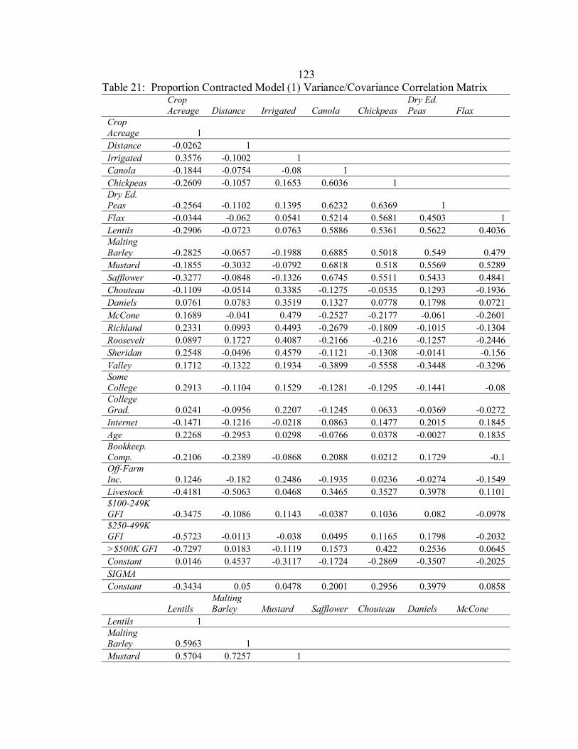
123

Table 21: Proportion Contracted Model (1) Variance/Covariance Correlation Matrix

Crop Acreage Distance Irrigated Canola Chickpeas

Dry Ed. Peas Flax

Crop Acreage 1 Distance -0.0262 1 Irrigated 0.3576 -0.1002 1 Canola -0.1844 -0.0754 -0.08 1 Chickpeas -0.2609 -0.1057 0.1653 0.6036 1 Dry Ed. Peas -0.2564 -0.1102 0.1395 0.6232 0.6369 1 Flax -0.0344 -0.062 0.0541 0.5214 0.5681 0.4503 1 Lentils -0.2906 -0.0723 0.0763 0.5886 0.5361 0.5622 0.4036 Malting Barley -0.2825 -0.0657 -0.1988 0.6885 0.5018 0.549 0.479 Mustard -0.1855 -0.3032 -0.0792 0.6818 0.518 0.5569 0.5289 Safflower -0.3277 -0.0848 -0.1326 0.6745 0.5511 0.5433 0.4841 Chouteau -0.1109 -0.0514 0.3385 -0.1275 -0.0535 0.1293 -0.1936 Daniels 0.0761 0.0783 0.3519 0.1327 0.0778 0.1798 0.0721 McCone 0.1689 -0.041 0.479 -0.2527 -0.2177 -0.061 -0.2601 Richland 0.2331 0.0993 0.4493 -0.2679 -0.1809 -0.1015 -0.1304 Roosevelt 0.0897 0.1727 0.4087 -0.2166 -0.216 -0.1257 -0.2446 Sheridan 0.2548 -0.0496 0.4579 -0.1121 -0.1308 -0.0141 -0.156 Valley 0.1712 -0.1322 0.1934 -0.3899 -0.5558 -0.3448 -0.3296 Some College 0.2913 -0.1104 0.1529 -0.1281 -0.1295 -0.1441 -0.08 College Grad. 0.0241 -0.0956 0.2207 -0.1245 0.0633 -0.0369 -0.0272 Internet -0.1471 -0.1216 -0.0218 0.0863 0.1477 0.2015 0.1845 Age 0.2268 -0.2953 0.0298 -0.0766 0.0378 -0.0027 0.1835 Bookkeep. Comp. -0.2106 -0.2389 -0.0868 0.2088 0.0212 0.1729 -0.1 Off-Farm Inc. 0.1246 -0.182 0.2486 -0.1935 0.0236 -0.0274 -0.1549 Livestock -0.4181 -0.5063 0.0468 0.3465 0.3527 0.3978 0.1101 $100-249K GFI -0.3475 -0.1086 0.1143 -0.0387 0.1036 0.082 -0.0978 $250-499K GFI -0.5723 -0.0113 -0.038 0.0495 0.1165 0.1798 -0.2032 >$500K GFI -0.7297 0.0183 -0.1119 0.1573 0.422 0.2536 0.0645 Constant 0.0146 0.4537 -0.3117 -0.1724 -0.2869 -0.3507 -0.2025 SIGMA Constant -0.3434 0.05 0.0478 0.2001 0.2956 0.3979 0.0858

Lentils Malting Barley Mustard Safflower Chouteau Daniels McCone

Lentils 1 Malting Barley 0.5963 1 Mustard 0.5704 0.7257 1

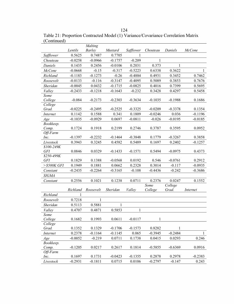
124

Table 21: Proportion Contracted Model (1) Variance/Covariance Correlation Matrix (Continued)

Lentils Malting Barley Mustard Safflower Chouteau Daniels McCone

Safflower 0.5625 0.7487 0.7705 1 Chouteau -0.0258 -0.0966 -0.1757 -0.209 1 Daniels 0.1435 0.2456 -0.0106 0.2031 0.373 1 McCone -0.0668 -0.15 -0.317 -0.5223 0.6338 0.3622 1 Richland -0.1183 -0.1273 -0.26 -0.4884 0.4931 0.3452 0.7462 Roosevelt -0.0133 -0.116 -0.3147 -0.4095 0.5089 0.3853 0.7676 Sheridan -0.0045 0.0432 -0.1715 -0.0825 0.4016 0.7399 0.5695 Valley -0.2433 -0.1218 -0.1643 -0.232 0.3428 0.4297 0.5458 Some College -0.084 -0.2173 -0.2303 -0.3634 -0.1035 -0.1988 0.1686 College Grad. -0.0225 -0.2495 -0.2525 -0.3325 -0.0209 -0.3378 0.1354 Internet 0.1142 0.1588 0.341 0.1809 -0.0246 0.036 -0.1196 Age -0.1035 -0.0929 0.0697 -0.0811 -0.026 -0.0195 -0.0185 Bookkeep. Comp. 0.1724 0.1918 0.2199 0.2746 0.3787 0.3595 0.0952 Off-Farm Inc. -0.1397 -0.2232 -0.1464 -0.3848 0.1779 -0.3267 0.3858 Livestock 0.3943 0.3245 0.4582 0.5489 0.1697 0.2402 -0.1257 $100-249K GFI 0.0846 0.0329 -0.1433 -0.1571 0.5494 -0.0975 0.4373 $250-499K GFI 0.1829 0.1388 -0.0568 0.0192 0.546 -0.0761 0.2912 >$500K GFI 0.1949 0.1881 0.0662 0.2328 0.3014 -0.117 -0.0935 Constant -0.2435 -0.2264 -0.3165 -0.108 -0.4436 -0.242 -0.3686 SIGMA Constant 0.2556 0.1021 0.1238 0.0711 0.2376 0.0247 0.1552

Richland Roosevelt Sheridan Valley Some College

College Grad. Internet

Richland 1 Roosevelt 0.7218 1 Sheridan 0.5113 0.5881 1 Valley 0.4707 0.4871 0.5853 1 Some College 0.1682 0.1993 0.0611 -0.0117 1 College Grad. 0.1352 0.1329 -0.1706 -0.1573 0.8282 1 Internet 0.2378 -0.1164 -0.1145 0.065 -0.3945 -0.2484 1 Age -0.0052 -0.219 0.0711 0.1738 0.0415 0.0293 0.246 Bookkeep. Comp. -0.1205 0.0217 0.2617 0.1814 -0.5855 -0.6369 0.0916 Off-Farm Inc. 0.1697 0.1731 -0.0423 -0.1355 0.2878 0.2978 -0.2383 Livestock -0.2931 -0.1811 0.0715 0.0106 -0.2797 -0.147 0.243

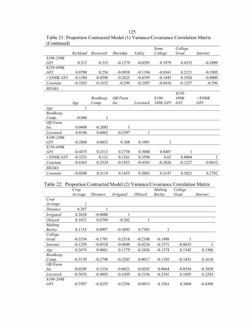
125

Table 21: Proportion Contracted Model (1) Variance/Covariance Correlation Matrix (Continued)

Richland Roosevelt Sheridan Valley Some College

College Grad. Internet

$100-249K GFI 0.213 0.315 -0.1279 -0.0293 0.1979 0.4352 -0.2889 $250-499K GFI 0.0708 0.256 -0.0938 -0.1194 -0.0361 0.2121 -0.1905 >$500K GFI -0.1584 -0.0396 -0.2623 -0.4395 -0.1443 0.1926 -0.0809 Constant -0.3263 -0.1632 -0.299 -0.2507 -0.0416 -0.1257 -0.396 SIGMA

Age Bookkeep. Comp.

Off-Farm Inc. Livestock

$100-249K GFI

$250-499K GFI

>$500K GFI

Age 1 Bookkeep. Comp. -0.046 1 Off-Farm Inc. 0.0408 -0.2083 1 Livestock 0.0196 0.6062 -0.2397 1 $100-249K GFI -0.2868 0.0032 0.368 0.1091 1 $250-499K GFI -0.4475 0.2313 0.2758 0.3008 0.8407 1 >$500K GFI -0.3251 0.121 0.1261 0.3598 0.65 0.8004 1 Constant -0.6363 -0.2524 -0.1853 -0.4363 -0.2026 -0.1227 -0.0632 SIGMA Constant -0.0208 0.2119 0.1455 0.2002 0.2147 0.3021 0.2782

Table 22: Proportion Contracted Model (2) Variance/Covariance Correlation Matrix

Crop Acreage Distance Irrigated Oilseed

Malting Barley

College Grad. Internet

Crop Acreage 1 Distance 0.287 1 Irrigated 0.2628 -0.0088 1 Oilseed 0.1072 0.0799 -0.202 1 Malting Barley 0.1135 0.0997 -0.3693 0.7383 1 College Grad. -0.3354 -0.1791 0.2518 -0.2108 -0.1498 1 Internet -0.1259 -0.0524 -0.0849 -0.0234 -0.1571 -0.0635 1Age 0.2674 0.0061 0.1179 -0.2426 -0.1374 0.1542 0.1306 Bookkeep. Comp. -0.3139 -0.2798 -0.2245 0.0017 -0.1192 -0.1431 0.1618 Off-Farm Inc. -0.0249 -0.3334 -0.0621 -0.0292 0.0664 -0.0554 -0.3839 Livestock -0.5676 -0.4892 -0.1039 -0.2156 -0.2341 0.1695 0.2243 $100-249K GFI -0.5507 -0.4255 -0.2356 -0.0913 0.1563 0.3868 -0.4309

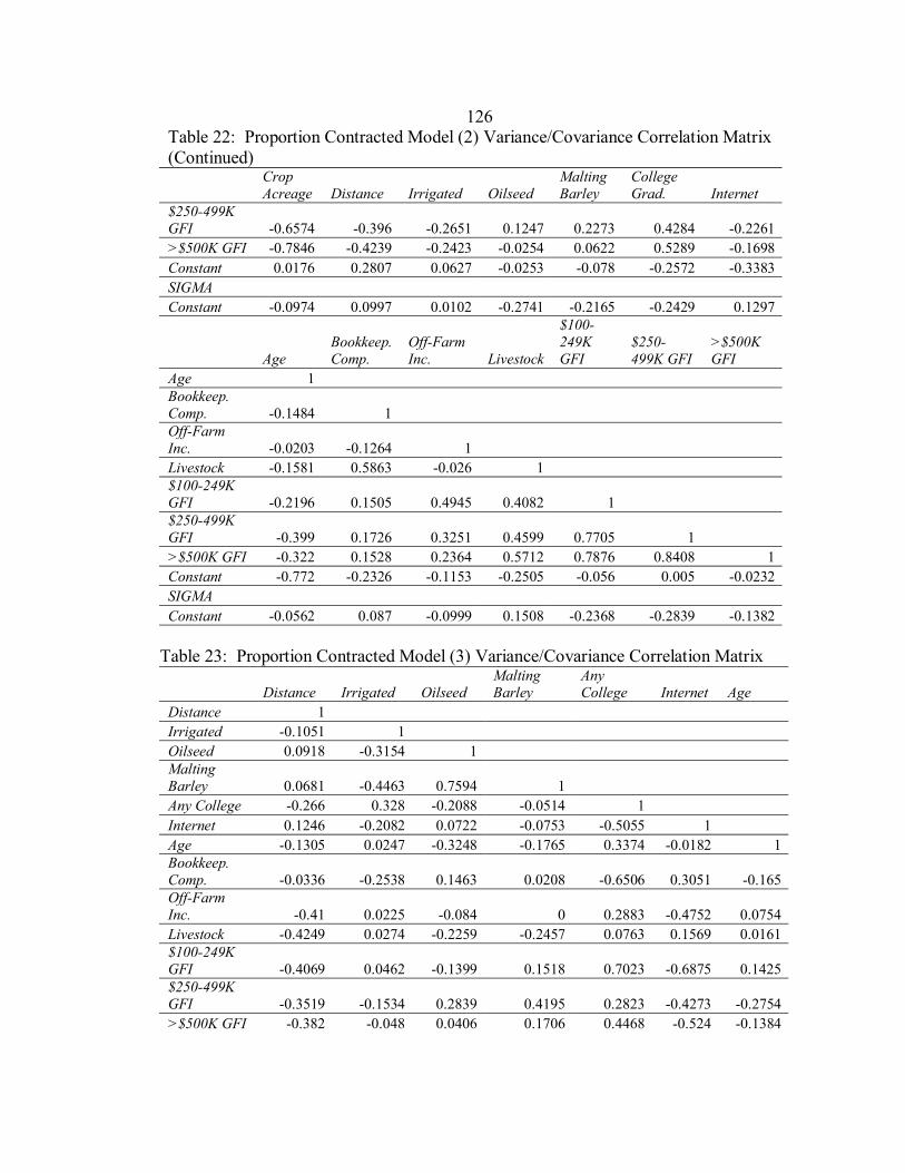
126

Table 22: Proportion Contracted Model (2) Variance/Covariance Correlation Matrix (Continued)

Crop Acreage Distance Irrigated Oilseed

Malting Barley

College Grad. Internet

$250-499K GFI -0.6574 -0.396 -0.2651 0.1247 0.2273 0.4284 -0.2261 >$500K GFI -0.7846 -0.4239 -0.2423 -0.0254 0.0622 0.5289 -0.1698 Constant 0.0176 0.2807 0.0627 -0.0253 -0.078 -0.2572 -0.3383 SIGMA Constant -0.0974 0.0997 0.0102 -0.2741 -0.2165 -0.2429 0.1297

Age Bookkeep. Comp.

Off-Farm Inc. Livestock

$100-249K GFI

$250-499K GFI

>$500K GFI

Age 1 Bookkeep. Comp. -0.1484 1 Off-Farm Inc. -0.0203 -0.1264 1 Livestock -0.1581 0.5863 -0.026 1 $100-249K GFI -0.2196 0.1505 0.4945 0.4082 1 $250-499K GFI -0.399 0.1726 0.3251 0.4599 0.7705 1 >$500K GFI -0.322 0.1528 0.2364 0.5712 0.7876 0.8408 1Constant -0.772 -0.2326 -0.1153 -0.2505 -0.056 0.005 -0.0232 SIGMA Constant -0.0562 0.087 -0.0999 0.1508 -0.2368 -0.2839 -0.1382

Table 23: Proportion Contracted Model (3) Variance/Covariance Correlation Matrix

Distance Irrigated Oilseed Malting Barley

Any College Internet Age

Distance 1 Irrigated -0.1051 1 Oilseed 0.0918 -0.3154 1 Malting Barley 0.0681 -0.4463 0.7594 1 Any College -0.266 0.328 -0.2088 -0.0514 1 Internet 0.1246 -0.2082 0.0722 -0.0753 -0.5055 1 Age -0.1305 0.0247 -0.3248 -0.1765 0.3374 -0.0182 1Bookkeep. Comp. -0.0336 -0.2538 0.1463 0.0208 -0.6506 0.3051 -0.165 Off-Farm Inc. -0.41 0.0225 -0.084 0 0.2883 -0.4752 0.0754 Livestock -0.4249 0.0274 -0.2259 -0.2457 0.0763 0.1569 0.0161 $100-249K GFI -0.4069 0.0462 -0.1399 0.1518 0.7023 -0.6875 0.1425 $250-499K GFI -0.3519 -0.1534 0.2839 0.4195 0.2823 -0.4273 -0.2754 >$500K GFI -0.382 -0.048 0.0406 0.1706 0.4468 -0.524 -0.1384

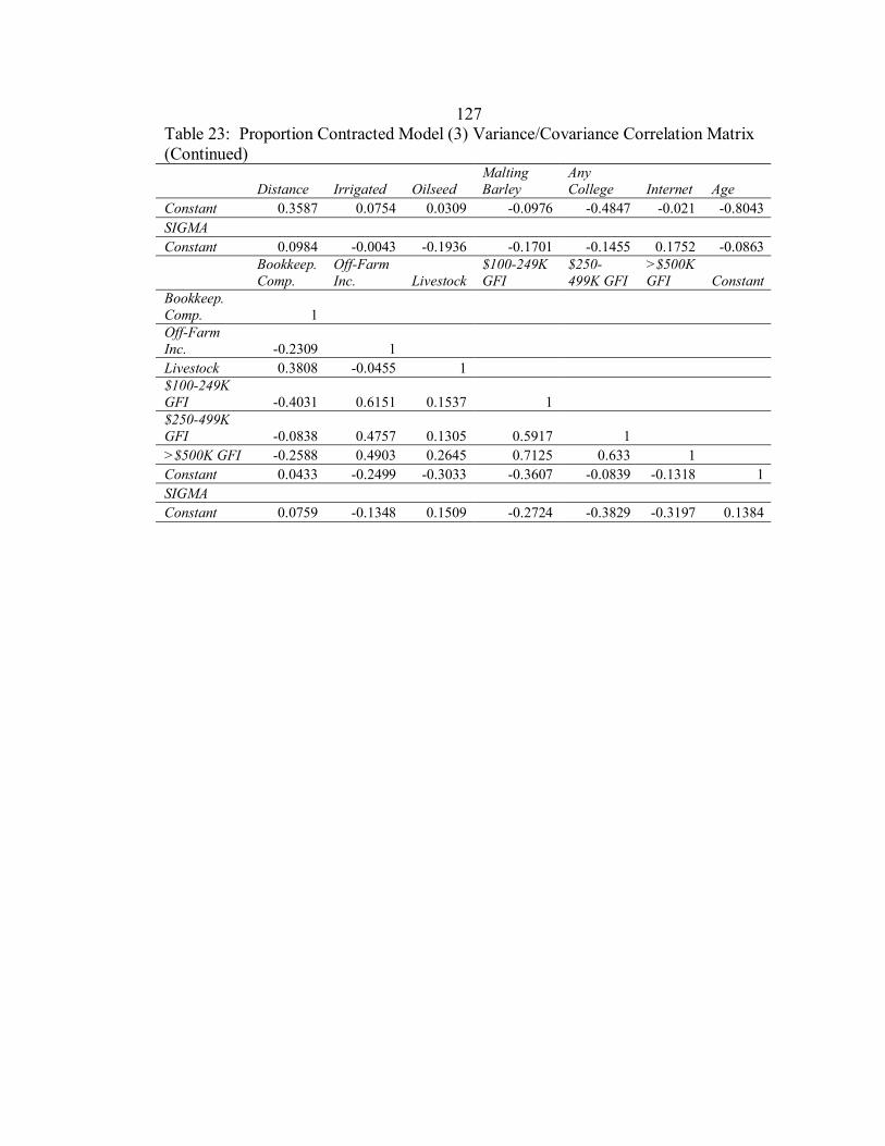
127

Table 23: Proportion Contracted Model (3) Variance/Covariance Correlation Matrix (Continued)

Distance Irrigated Oilseed Malting Barley

Any College Internet Age

Constant 0.3587 0.0754 0.0309 -0.0976 -0.4847 -0.021 -0.8043 SIGMA Constant 0.0984 -0.0043 -0.1936 -0.1701 -0.1455 0.1752 -0.0863

Bookkeep. Comp.

Off-Farm Inc. Livestock

$100-249K GFI

$250-499K GFI

>$500K GFI Constant

Bookkeep. Comp. 1 Off-Farm Inc. -0.2309 1 Livestock 0.3808 -0.0455 1 $100-249K GFI -0.4031 0.6151 0.1537 1 $250-499K GFI -0.0838 0.4757 0.1305 0.5917 1 >$500K GFI -0.2588 0.4903 0.2645 0.7125 0.633 1 Constant 0.0433 -0.2499 -0.3033 -0.3607 -0.0839 -0.1318 1SIGMA Constant 0.0759 -0.1348 0.1509 -0.2724 -0.3829 -0.3197 0.1384