Embed Size (px)
Citation preview

Market Size, Innovation, and the EconomicEffects of an Epidemic∗
Domenico FerraroArizona State University
Pietro F. PerettoDuke University
October 12, 2020
Abstract
We develop a framework for the analysis of the economic effects of an epidemic thatincorporates firm-specific innovation and endogenous entry. Transition dynamics ischaracterized by two differential equations describing the evolution of the mass ofsusceptible in the population and the ratio of the population to the mass of firms.An epidemic propagates through the economy via changes in market size that re-duce incentives to enter the market and to undertake innovative activity. We evaluatestate-dependent interventions involving policy rules based on tracking susceptible orinfected. Simple policy rules are announced at the time of the outbreak and anchorsprivate sector’s expectations about the time path of the intervention, including theend date. Welfare gains/losses relative to the do-nothing scenario are computed ac-counting for transition dynamics.
JEL Classification: E23; E24; E62; O30; O40.Keywords: Epidemic; Growth; Productivity; Market structure; Entry; Innovation.
∗Ferraro: Department of Economics, W.P. Carey School of Business, Arizona State University, POBox 879801, Tempe, AZ 85287-9801, United States (e-mail: [email protected]); Peretto: De-partment of Economics, Duke University, Box 90097, Durham, NC 27708-0097, United States (e-mail:[email protected]). First draft: September 17, 2020.

1 Introduction
The spread of infectious diseases (“epidemics”) has ravaged humanity throughout its
history, often leaving indelible scars. The Spanish Flu of 1918-20 and the most recent
COVID-19 are only two examples of a long list of severe epidemics involving substantial
disruptions in economy activity. Evaluating the economic consequences of an epidemic,
including the trade-offs involved in intervention policies, requires a structural model of
the economy that allows for counterfactual analysis under alternative policy scenarios.
A recent and fast growing literature tackles these questions in the context of general
equilibrium models in which an epidemic, and the policy response to it, affects economy
activity through changes in market hours worked, consumption, and physical capital
investment (Eichenbaum, Rebelo and Trabandt, 2020a,b,c). In these economic models,
augmented with epidemiological models of an infectious disease, the immediate effect of
an epidemic is a reduction in the amount of labor services supplied to the market, akin to
a negative “labor supply shock,” which can be amplified by a lockdown policy. How and
the extent to which this initial epidemic shock propagates through the economy depends
on the specific features of the economic environment and mechanisms at play (see Section
2 for a literature review).
The objective of this paper is to build a tractable, dynamic general equilibrium model
to address important, yet overlooked, questions relating the spread of an epidemic to
market structure, innovation, and productivity growth. To achieve this goal, we integrate
a standard Susceptible-Infected-Recovered-Deceased (SIRD) model of infectious diseases
into a growth model featuring variety expansion and firm-specific cost-reducing inno-
vation (Peretto and Connolly, 2007). Endogenous market structure propagates the epi-
demic shock, leading to a very persistent response of the growth rate, featuring a sharp
initial drop followed by a prolonged hump-shaped reversion to the initial steady state.
(The long-run growth rate remains unchanged, as we work with a growth model without
strong scale effect.)
Methodologically, we propose a new concept of “infection function,” which links the
fraction of infected in the population to the fraction of susceptible. Using this concept,
the dynamical system describing the equilibrium dynamics of the economy, in and out of
the steady state, reduces to two differential equations. Solving for the equilibrium of our
growth model is easy despite the highly nonlinear structure of the dynamical system.
1

In our model, a market size effect is key to the propagation of an epidemic. Indeed,
an epidemic manifests itself as a shock to market size. Hump-shaped dynamics in the
fraction of infected in the population due to the spread of the disease translates into U-
shaped dynamics in the amount of labor services available for production. This leads to
a drop in per capita consumption expenditure which initiates transition dynamics fueled
by changes in firms’ incentives to enter the market and incumbents’ innovative activity.
More specifically, the model features highly non-linear transition dynamics: depending
on the magnitude of the fall in expenditure, the economy may experience a prolonged
period of net firm exit with a shutdown of innovation altogether. In this extreme sce-
nario, growth in total factor productivity (TFP) does not only slow down, but it turns to
negative, implying a temporary fall in the level of TFP. In fact, if one allows for the possi-
bility of death as in the standard SIRD case, and so a permanent reduction in population,
the loss of product variety is permanent because the new steady-state associated with a
smaller population size exhibits fewer firms and so less product variety.
We use the model to study policy interventions that operate through a reduction in
the transmission rate of the epidemic, as well as a direct reduction in the labor input,
mimicking the effect of a mandated lockdown. Such interventions are state-dependent
and involve policy rules based on tracking the fraction of susceptible or infected in the
population, akin to the Taylor’s rule for monetary policy. Policy rules are announced at
the time of the outbreak and anchors private sector’s expectations about the time path
and the end date of the intervention. We restrict our attention to simple rules to retain
analytical tractability, and compute welfare gains/losses relative to a do-nothing scenario,
accounting for transition dynamics.
Numerical simulations illustrate a sharp policy trade-off. Slowing down contagion
amounts to engineering a deeper recession relative to the do-nothing scenario. Interven-
tions generally induce a persistent slowdown in aggregate productivity growth. Depend-
ing on the severity and duration of the intervention, transition dynamics may feature
prolonged periods of net exit with negative TFP growth.
The paper is structured as follows. Section 2 discusses the related literature. In Section
3, we present the basic growth model, into which we embed the SIRD epidemiological
model. In Sections 4 and 5, we analyze the equilibrium dynamics of the model pre- and
post-infection. Section 6 discusses the effects of policy intervention. Section 7 presents
numerical results. Section 8 concludes. Appendices A, B, and C contain details on model’s
2
derivations, parametrization, and additional results.
2 Related Literature
This papers adds to the theoretical literature studying the economic effects of infectious
disease. Goenka, Liu and Nguyen (2014) is an early (pre-COVID-19) contribution that in-
tegrates epidemiological dynamics into a neoclassical growth model with investment in
health which affects the recovery rate from the disease. They establish that a disease-free
steady state can coexists with a disease-endemic steady state in which health expenditure
is either positive or zero depending on parameter values. Goenka and Liu (2020) extend
this framework by allowing for investment in human capital. A disease-free balanced
growth path with sustained economic growth coexists with multiple disease-endemic
balanced growth paths in which the economy either grows at a slower rate or remains
stuck in a poverty trap without human capital accumulation. Greenwood et al. (2019)
quantitatively evaluate the economic impact of the HIV/AIDS epidemic in Malawi using
a general equilibrium search model of sexual behavior.
The literature studying different aspects of the COVID-19 epidemics is growing at a
surprisingly fast rate.1 Early contributions by Eichenbaum, Rebelo and Trabandt (2020a),
Eichenbaum, Rebelo and Trabandt (2020b), and Eichenbaum, Rebelo and Trabandt (2020c)
study the economic consequences of COVID-19, testing and quarantining policies in the
context of a neoclassical growth model (with/without monopolistic competition) and of a
New Keynesian model with sticky prices. The main idea in these papers is that individual
consumption and work decisions affect the transmission rate of the epidemic, creating an
infection externality. The competitive equilibrium is thus not Pareto optimal. Testing and
quarantining can improve upon the laissez-faire outcome.
Relative to these papers, we ask a different question and study a new mechanism in
which market structure and transition dynamics take center stage. Notably, transition
dynamics of economic variables is considerably slower than epidemiological dynamics.
Through changes in the fraction of infected in the population, an epidemic leads to a fall in
1A partial list includes: Acemoglu et al. (2020), Alvarez, Argente and Lippi (2020), Atkeson (2020),Barro, Ursua and Weng (2020), Bethune and Korinek (2020), Bognanni et al. (2020), Brotherhood et al.(2020), Farboodi, Jarosch and Shimer (2020), Glover et al. (2020), Jones, Philippon and Venkateswaran(2020), Krueger, Uhlig and Xie (2020). See https://www.nber.org/wp_covid19.html and https://voxeu.org/pages/covid-19-page for an extensive list of NBER/CEPR working papers on COVID-related research.
3

expenditure which shrinks the size of the market served by producers. This market-size
effect reduces incentives to entry and incumbents’ cost-reducing activity, leading to the
prolonged hump-shaped response of the growth rate described above. The source of this
shape is the internal propagation mechanism at play in the economic block of the model,
which yields that epidemiological and economic variables move at rather different speed.
Further, we propose state-dependent intervention rules based on tracking susceptible or
infected in the population, that naturally lend themselves for welfare analysis. Such rules
are an essential part of the definition of equilibrium.
3 Environment
To streamline exposition, we keep the description of the environment for the benchmark
model without infection to a minimum. We refer the reader to Appendix A for further
details.
Preferences and budget set The economy is populated by a representative household
with L(t) infinitely-lived members, each endowed with one unit of time per period. Labor
supply is inelastic, so that household’s labor supply equal L(t) at all times. Preferences
are described by
U(t) =∫ ∞
te−ρ(s−t)L (s) log [C(s)] ds, ρ > 0, (1)
where C =[∫ N
0 (Xi/L)ε−1
ε di] ε
ε−1is a CES aggregator of differentiated consumer goods
Xi, with elasticity of substitution ε > 1, and N is the mass of consumer goods available
for purchase. The budget constraint is A = rA + wL − Y, where A is assets yielding a
rate of return r, w is the wage, Y =∫ N
0 piXidi = pCC is consumption expenditures, and
pC =(∫ N
0 p1−εi di
) 11−ε is a Dixit-Stiglitz price index.
The household’s maximization problem yields a standard Euler equation,
r = rA ≡ ρ +YY− L
L, (2)
which gives the household’s reservation rate of return on savings, rA, and a downward-
4
sloping demand for differentiated goods,
Xi = Yp−ε
i∫ N0 p1−ε
j dj. (3)
Production and innovation Firm i produces Xi units of the differentiated good using
LXi units of labor and the technology Xi = Zθi(
LXi − φ), with 0 < θ < 1, and φ > 0, where
Zi is the firm-specific stock of knowledge. Firm-specific knowledge evolves according to
Zi = αKLσZi
L1−σZ , with α > 0, and 0 < σ ≤ 1, where LZi is R&D labor, K = (1/N)
∫ N0 Zjdj,
and LZ = (1/N)∫ N
0 LZj dj. An incumbent firm i chooses the paths of the unit price pi and
R&D labor LZi to maximize the value of the firm,
Vi (t) =∫ ∞
te−∫ s
t [r(v)+δ]vΠi(s)ds, (4)
where Πi ≡ (pi − wZ−θi )Xi − wφ− wLZi is profits and δ > 0 is a “death shock.”
An entrant pays a sunk cost βY/N = wLNi and creates value Vi. Hence, free-entry
implies Vi = βY/N. One can think of the entry process in terms of an underlying entry
technology (as typically done in literature):
N =
(wβY
N)
LN − δN. (5)
4 Pre-infection Equilibrium Dynamics
We now turn to the general equilibrium of the benchmark model without infection. As
the equilibrium of the economy is symmetric, henceforth, we drop the subscript i such
that, for example, X = Xi indicates both firm-level and average production of consumer
goods. Labor is the numéraire, i.e., we set w ≡ 1. The value of the household’s portfolio
equals the value of securities issued by firms, A = NV. (Note that when free entry holds,
NV = βY, otherwise NV < βY.) Assets market equilibrium requires rates of return
equalization, i.e., r = rA = rZ = rN, where rZ and rN are the rates of return to cost
5

reduction and to entry,
r = rZ ≡ α
[Yσθ(ε− 1)
εN− w
LZ
N
]+
ww− δ, (6)
r = rN ≡1β
[1ε− N
Y
(φ + w
LZ
N
)]+
YY− N
N− δ. (7)
Let y ≡ Y/L denote per capita expenditure, and x ≡ L/N the ratio of population to
the mass of firms. When free entry holds, expenditures per capita y and rate of return r
are constant and equal to
y = y∗ ≡ 11− βρ
, and r = ρ. (8)
When free entry does not hold, instead,
y =ε
ε− 1
(1− φ
x
), and r = ρ +
yy
. (9)
Pre-infection transition dynamics Transition dynamics of the pre-infection economy is
characterized by one differential equation for the population-to-firms ratio, x:
x =
δx if φ ≤ x ≤ xN1−βρ
β φ−(
1βε − ρ− δ
)x if xN < x ≤ xZ
1−βρβ
(φ− ρ+δ
α
)−[
1−σθ(ε−1)βε − ρ− δ
]x if x > xZ
, (10)
where the thresholds xN and xZ are defined as
xN ≡(1− βρ) εφ
1− ρβε, and xZ ≡
(1− βρ) (ρ + δ)
σαθ ε−1ε
. (11)
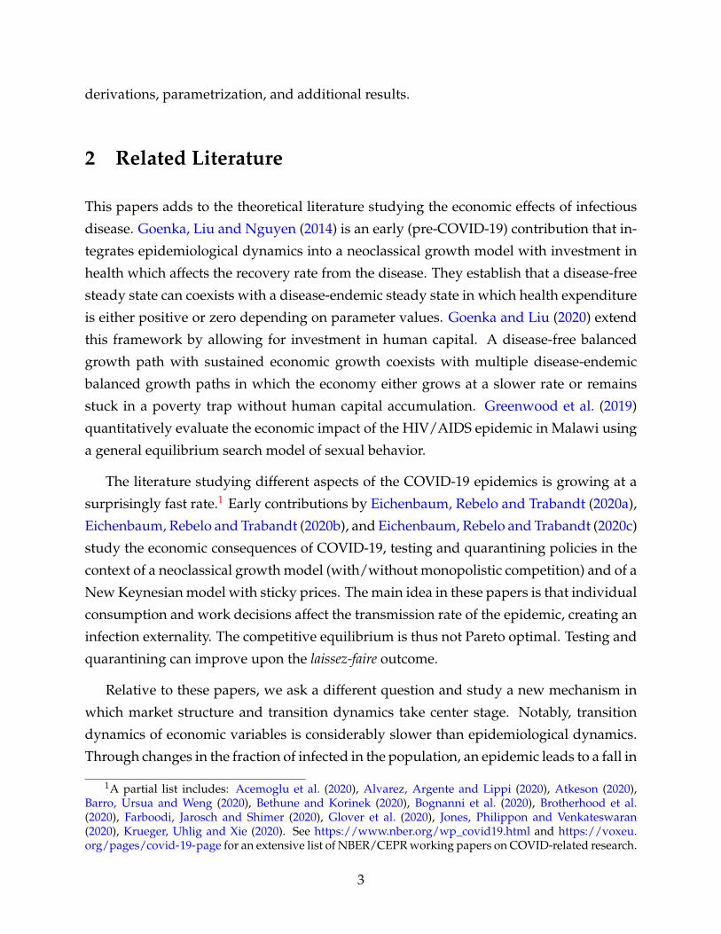
As illustrated by Figure 1, the transition dynamics features three regions: (i) net firms’
exit with zero R&D labor (φ ≤ x ≤ xN); (ii) gross firms’ entry with zero R&D labor
(xN < x ≤ xZ); (iii) gross firms’ entry with positive R&D labor (x > xZ). On the left of
the threshold xN, firm size x ≤ xN is “too small,” implying net firms’ exit. As a result,
the population-to-firms ratio grows at rate δ of firms’ exit, which contributes to increase
profitability. As x crosses xN, in the region xN < x ≤ xZ, firms enter, which slows
down the growth rate of firm size. In this region, there is no accumulation of knowledge.
6

Finally, on the right of the threshold xZ, when average firm size becomes “large enough,”
firm entry and knowledge accumulation coexist.
Using the equation for the rate of return to cost reduction (6), we obtain the growth
rate of the stock of knowledge:
z ≡ ZZ
= αLZ
N=
0 if x ≤ xZ
x · yασθ(
ε−1ε
)− r− δ if x > xZ
. (12)
Finally, using the Euler equation (2), and the rate of return to entry (7), we obtain the
growth rate of the mass of firms,
n ≡ NN
=1β
[1ε− 1
xy
(φ +
LZ
N
)]− ρ +
LL− δ. (13)
Pre-infection balanced growth path Under the following conditions on parameters,
αφ > ρ + δ, (14)
(ρ + δ) β +σθ (ε− 1)
ε<
1ε< (ρ + δ) β +
(αφ
ρ + δ
)σθ (ε− 1)
ε, (15)
the model exhibits a balance growth path (BGP) with endogenous growth, along which
x, z ≡ Z/Z, and the mass of firms, N, take the following steady-state values:
x∗ =(1− βρ) ε
(φ− ρ+δ
α
)1− σθ (ε− 1)− (ρ + δ) βε
, (16)
z∗ =φα− (ρ + δ)
1− σθ (ε− 1)− (ρ + δ) βεθ (ε− 1)− (ρ + δ) , (17)
N∗ =
1− σθ (ε− 1)− (ρ + δ) βε
ε(
φ− ρ+δα
)(1− βρ)
L. (18)
Note that along a BGP, x∗ and z∗ are independent of the population level L. This is an
important feature of the model that comes from the property that the mass of firms N∗ is
proportional to L. Because of this property, the model does not suffer from the so-called
“scale effect,” at work in the first-generation models of endogenous growth à la Romer
(1990). We stress that the proportionality between number of firms and the population
7

level is a BGP phenomenon, which breaks when the economy is in transition dynamics.
ẋ
xx*x xN Z
Figure 1: Pre-infection Equilibrium Dynamics
Notes: The figure depicts the equilibrium dynamics of the population-to-firms ratio as implied bythe piecewise differential equation (10), where the thresholds xN and xZ are as defined in (11),and the steady-state value x∗ is as in (16).
Given the formula for the price index pC =[∫ N
0 p1−εi di
] 11−ε , along a BGP, real per
capita consumption expenditure is
y∗
pC=
y∗
c∗· Zθ N
1ε−1 , (19)
where c∗ = εε−1 · w captures “static” drivers of the price index, i.e., those unrelated to
endogenous technological change. (Recall the normalization w = 1.)
8
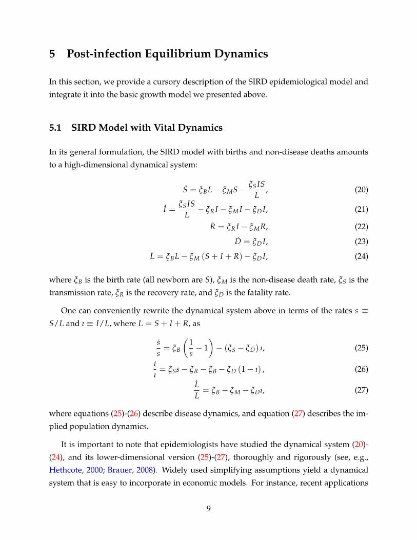
5 Post-infection Equilibrium Dynamics
In this section, we provide a cursory description of the SIRD epidemiological model and
integrate it into the basic growth model we presented above.
5.1 SIRD Model with Vital Dynamics
In its general formulation, the SIRD model with births and non-disease deaths amounts
to a high-dimensional dynamical system:
S = ξBL− ξMS− ξS ISL
, (20)
I =ξS IS
L− ξR I − ξM I − ξD I, (21)
R = ξR I − ξMR, (22)
D = ξD I, (23)
L = ξBL− ξM (S + I + R)− ξD I, (24)
where ξB is the birth rate (all newborn are S), ξM is the non-disease death rate, ξS is the
transmission rate, ξR is the recovery rate, and ξD is the fatality rate.
One can conveniently rewrite the dynamical system above in terms of the rates s ≡S/L and ı ≡ I/L, where L = S + I + R, as
ss= ξB
(1s− 1)− (ξS − ξD) ı, (25)
ıı= ξSs− ξR − ξB − ξD (1− ı) , (26)
LL= ξB − ξM − ξDı, (27)
where equations (25)-(26) describe disease dynamics, and equation (27) describes the im-
plied population dynamics.
It is important to note that epidemiologists have studied the dynamical system (20)-
(24), and its lower-dimensional version (25)-(27), thoroughly and rigorously (see, e.g.,
Hethcote, 2000; Brauer, 2008). Widely used simplifying assumptions yield a dynamical
system that is easy to incorporate in economic models. For instance, recent applications
9

of the epidemiological framework to economics typically set ξB = ξM = 0. This is the
case of no vital dynamics.
s
s
1s∞ s
.
i=0.
trajectory =
infection function i(s)
herd
(a) SIRD model
s
s
1s∞ sherd
.i=0.
trajectory =
infection function i(s)
(b) SIR model
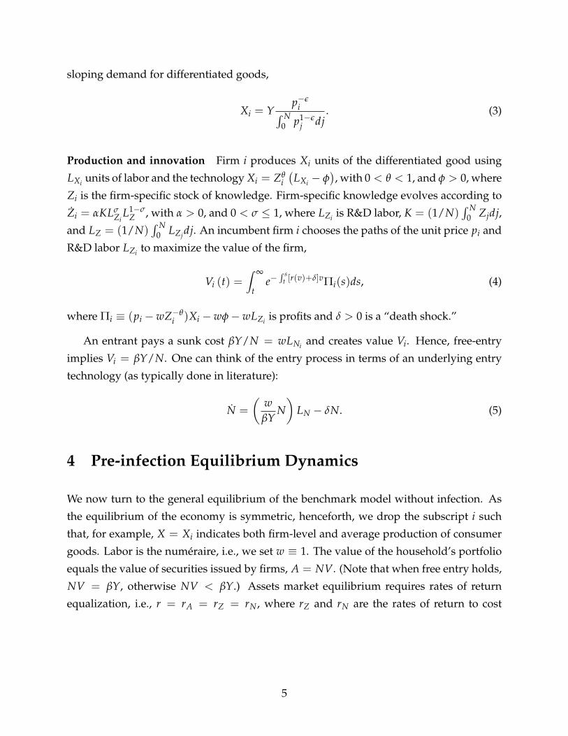
Figure 2: Epidemiological Models of Infectious Diseases
Notes: The figures shows the phase diagram for the SIRD model (top panel) and for the SIR model(bottom panel).
10

Infection function Figures 2a-2b depict the phase diagrams for the SIRD and SIR model,
respectively. In each case, for the initial state (s0, ı0), with ı0 ≈ 0 and s0 ≈ 1, there exists
a hump-shaped trajectory ı (s) that we interpret as “infection function.” Next, we leverage
this concept of infection function to integrate epidemiology into an economic model.
To this goal, we use ı(s) to compress the epidemic model to one equation:
ss= ξB
(1s− 1)− (ξS − ξD) ı (s) . (28)
In macroeconomics jargon, for given (ξB, ξM, ξS, ξD), equation (28) represents the law of
motion of the “epidemic shock.”
Next, to solve for ı(s) in (28), we take the ratio of equations (25) and (26), which gives
the partial differential equation (PDE),
dıds
=ξSs− ξR − ξD − ξB + ξDı
ξB
(1s − 1
)− (ξS − ξD) ı
( ıs
). (29)
The solution to this PDE is indeed well-known in the epidemiological literature (see, e.g.,
Brauer, 2008).
Infection function: SIRD. For ξB = ξM = 0, the PDE (29) reduces to the d’Alembert’s
equation
dıds
=1s
ξR + ξD(1− ı)ξS − ξD
− ξS
ξS − ξD. (30)
Solving the PDE (30) with the boundary conditions ı (0) = ı0 and s (0) = 1− ı0 ≡ s0
yields the infection function
ı (s) =ξR
ξD
1−(
ss0
)− ξDξS−ξD
+ 1− s, (31)
which is a hump-shaped function with s∞ ≡ arg solve {ı (s) = 0} > 0. Figure 3a depicts
the infection function (31) for the SIRD model.2
Infection function: SIR. For ξB = ξM = ξD = 0 (i.e., constant population), the PDE (29)
2In the SIRD case, the epidemic shock that hits the economy is ss = − (ξS − ξD) ı (s).
11

s
i
1s∞0 sherd
(a) SIRD model
s
i
1s∞ 1/R00
(b) SIR model
Figure 3: Infection Function
Notes: The figures depicts the infection function for the SIRD model (top panel) and for the SIRmodel (bottom panel).
reduces to
dıds
=1
R0S− 1, R0 ≡
ξS
ξR. (32)
12

Solving the PDE (32) with boundary conditions ı (0) = ı0 and s (0) = 1− ı0 ≡ s0 yields
the infection function
ı (s) =1
R0log(
ss0
)+ 1− s, (33)
which is a hump-shaped function with s∞ ≡ arg solve {ı (s) = 0} > 0. Figure 3b depicts
the infection function (33) for the SIR model.3
5.2 Embedding the SIRD Model into the Growth Model
We now embed the SIRD model without vital dynamics (i.e., ξB = ξM = 0) into the basic
growth model. First, in the SIRD case with ξD > 0, the epidemic permanently removes
people from the economy leading to negative population growth:
LL= −ξDı (s) . (34)
Second, the disease temporarily removes people from the labor force, akin to a negative
“labor supply shock,”
LX + LZ + LN︸ ︷︷ ︸labor demand
(allocation)
= [1− ı (s)] L.︸ ︷︷ ︸labor supply
(participation)
(35)
Third, through the mortality rate ξD, the epidemic directly affects the discount rate of
utility flows:
L (t) u(t) = e−∫ t
0 ξDı(v)dv log C. (36)
Akin to the Yaari-Blanchard perpetual youth model, one can interpret discounting through
the term e−∫ t
0 ξDı(v)dv as an individual life expectancy effect: the disease can kill me, not
just my siblings.
3In the SIR case, the epidemic shock that hits the economy is ss = −ξSı (s).
13

5.2.1 Expenditures and Interest Rates
Per capita expenditures Overall, per capita consumption expenditure is decreasing in
the fraction of infected in the population, ı. In general equilibrium, an epidemic manifests
itself on the demand side of the economy, too, as a reduction in market size. Through this
channel, it alters firms’ incentives to enter the market and incumbents’ allocation of R&D
labor, initiating transition dynamics.
When free entry does not hold, per capita expenditure is
y (s, x) =ε
ε− 1
(1− φ
x
)[1− ı (s)] , (37)
which is U-shaped in s since the infection function ı(s) is humped-shaped in the fraction
of susceptible in population, s. On the other hand, when free entry holds, per capita
expenditure is
y (s) =1− ı (s)
1− [ρ + ξDı (s)] β. (38)
Assuming 1 > β (ρ + ξD) to guarantee existence for ı ∈ [0, 1], it implies dy/dı < 0. Again,
y is U-shaped in s since ı (s) is hump-shaped in s. Importantly, as ı goes from 0 to ı0 > 0,
an outbreak yields a fall in y at t = 0. As s falls throughout, y initially keeps falling, turns
around at the peak of epidemic and returns to y∗ from below.
Interest rates Log-differentiating the expression for y yields
yy= − 1− (ρ + ξD) β
1− [ρ + ξDı (s)] β· ı(s)
1− ı(s). (39)
Next, using the Euler equation, and the expression for ı gives an expression for the
interest rate:
r (s) = ρ− 1− (ρ + ξD) β
1− [ρ + ξDı (s)] β︸ ︷︷ ︸increasing in ı
· ı (s)1− ı (s)︸ ︷︷ ︸
increasing in ı
· [ξSs− ξR − ξD + ξDı (s)]︸ ︷︷ ︸increasing in ı
. (40)
A few remarks are in order here. (i) The interest rate is below ρ and decreasing in ı
14

when the term in square brackets on the right-hand side [·] ≡ [ξSs− ξR − ξD + ξDı (s)]
is larger than zero; and (ii) it is above ρ and increasing in ı when [·] < 0. The fraction of
infected ı (s) is decreasing in s for [·] > 0 and increasing in s when [·] < 0. As a result, the
interest rate r (s) is first hump- and then U-shaped in the fraction of susceptible, s. Since
initially [·] > 0, the outbreak yields a fall in r at t = 0. As s falls throughout, the interest
rate continues falling, it turns around at the peak of the epidemic, overshoots and finally
returns to ρ from above.
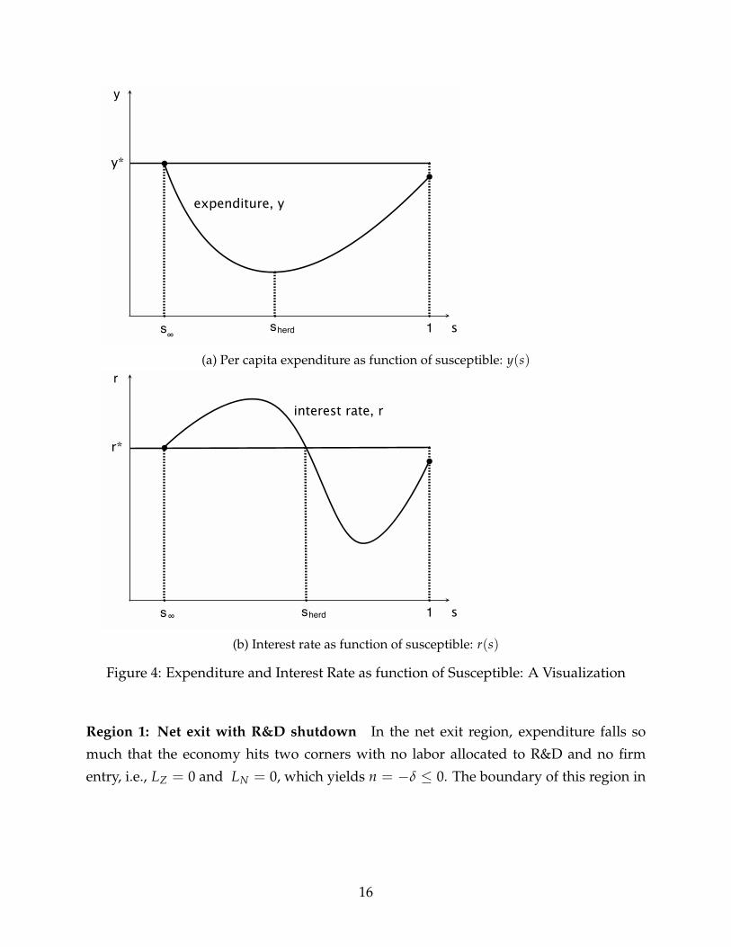
To visualize some of the qualitative features of the transition dynamics, Figures 4 and
5 show per capita expenditures and interest rate dynamics as a function of the fraction of
susceptible and time, respectively.
5.2.2 Market Structure, Productivity, and Welfare
Using the expressions for y(s) and r(s) in equations (38) and (40), respectively, the general-
equilibrium dynamics reduces to a tractable system of two differential equations: (i) the
first equation describes the evolution over time of the economic state variable of the
model, i.e. the ratio of the population to the mass of firms, x ≡ L/N; (ii) the second
equation describes the evolution of the epidemiological state variable, i.e. the fraction of
susceptible in the population, s.
Outbreak At t = 0, per capita expenditure y falls from its steady-state value y∗ to the
lower value associated with ı(s0) or ı0 for short:
y (s0) =1− ı0
1− (ρ + ξDı0) β< y∗. (41)
Such a drop in expenditure initiates transition dynamics, during which the economic state
variable follows
xx= −ξDı− n, (42)
with initial condition x0 = L0/N0 ≥ 0 and n ≡ N/N indicating the growth rate of the
mass of firms. The dynamical system features three regions that differ qualitatively in
terms of market structure and R&D labor allocations.
15
s
expenditure, y
y*
1s∞
y
sherd
(a) Per capita expenditure as function of susceptible: y(s)
s
interest rate, r
r*
1s∞
r
sherd
(b) Interest rate as function of susceptible: r(s)
Figure 4: Expenditure and Interest Rate as function of Susceptible: A Visualization
Region 1: Net exit with R&D shutdown In the net exit region, expenditure falls so
much that the economy hits two corners with no labor allocated to R&D and no firm
entry, i.e., LZ = 0 and LN = 0, which yields n = −δ ≤ 0. The boundary of this region in
16

time
expenditure, y
y*
y
(a) Per capita expenditure over time: y(t)
time
interest rate, r
r*
r
(b) Interest rate over time: r(t)
Figure 5: Expenditure and Interest Rate as function of Time: A Visualization
the x-dimension is determined by the following condition:
1− [ρ + ξDı (s)] β
1− ı (s)εφ ≤ x ≤ 1− [ρ + ξDı (s)] β
1ε − [ρ + ξDı (s)] β
· φ
1− ı (s). (43)
17

In this region, the dynamical system is
ss= − (ξS + ξD) ı (s) , (44)
xx= δ− ξDı (s) . (45)
Region 2: Gross entry with R&D shutdown The boundary of this region in the x-
dimension is determined by the following condition:
1− [ρ + ξDı (s)] β1ε − [ρ + ξDı (s)] β
· φ
1− ı (s)< x ≤ r (s) + δ
σαθ ε−1ε
· 1− [ρ + ξDı (s)] β
1− ı (s). (46)
In this region, the dynamical system is
ss= − (ξS + ξD) ı (s) , (47)
xx=
φ
βy (s)· 1
x− 1
βε+ ρ + δ. (48)
The underlying net entry process follows n = −x/x− ξDı (s).
Region 3: Gross entry with active R&D Finally, the boundary of the region featuring
gross entry with active R&D is determined by the following inequality:
x >r (s) + δ
σαθ ε−1ε
· 1− [ρ + ξDi (s)] β
1− i (s). (49)
In this region, the dynamical system is
ss= − (ξS + ξD) ı (s) , (50)
xx=
1βy (s)
(φ− r (s) + δ
α
)1x− 1− σθ (ε− 1)
βε+ ρ + δ. (51)
The underlying net entry process follows n = −x/x− ξDi (s) and knowledge growth
is positive and equal to z = x · ασθ ε−1ε y (s)− r (s)− δ > 0.
18

s
x
1
x*
s∞ s herd
(1,x*)
ẋ=0
Case a
Case b
Figure 6: Post-infection Dynamics
Notes: The figure depicts the phase diagram for the post-infection economy. On the x-axis, sdenotes the fraction of susceptible in the population; on the y-axis, x denotes the ratio of thepopulation to the mass of firms.
R&D labor allocation and TFP To provide some insight into the transition dynamics
implied by the model, Figure 6 illustrates two potential trajectories in the (s, x) space
for the case of next exit. The population-to-firms ratio, x, grows initially because of net
exit due to falling profitability caused by falling expenditure. Both y and r jump down
and initially follow U-shaped paths. The net effect can be a fall in knowledge growth,
z. Overall, the transition dynamics features an initial deceleration of firm productivity
growth with reversion to the long-run level. Possibly, a phase with zero firm growth.4
Such a temporary deceleration delivers a permanent TFP loss relative to the baseline
no-disease path. Note also that period of net exit means period of falling TFP. This is a
real loss, not just relative to the no-disease baseline (i.e., a “lost opportunity” loss). In
the SIRD case, the transition features overall net exit because the new steady state exhibit
fewer firms, i.e., N < N∗ due to a smaller population. This causes TFP to fall permanently.
In the SIR case instead, such an effect is only temporary.
4Formally, the constant population-to-firms ratio x ≥ 0 locus is (i) x ≤ εφ1−(ρ+δ)βε
· 1−[ρ+ξD ı(s)]β1−ı(s) for
Region 2 and (ii) x ≤ε(
φ− r(s)+δα
)1−σθ(ε−1)−(ρ+δ)βε
· 1−[ρ+ξD ı(s)]β1−ı(s) for Region 3.
19

Welfare Real expenditure per capita is equal to
C =y
pC=
(ε− 1
ε
)y · Zθ N
1ε−1︸ ︷︷ ︸
TFP
, (52)
which implies a utility flow of log C (t) = log(
ε−1ε
)+ log y (t)+ θ log Z (t)+ 1
ε−1 log N (t).
Further, normalizing log(
ε−1ε Zθ
0 N1
ε−10
)= 0, we rewrite the utility flow as
log C (t) = log y (t) + θ∫ t
0z (s) ds +
1ε− 1
∫ t
0n (s) ds. (53)
Importantly, in calculating the welfare integral in (1), effective discounting accounts
for fatality due to the spread of the epidemics:
exp{−ρt−
∫ t
0ξDi (s (v)) dv
}. (54)
6 Policy Intervention
In this section, we study policy interventions that operate through a reduction in the
transmission rate of the epidemic, which entails a reduction in the supply of labor, akin to
a lockdown. Let h ≥ 0 denote the policy variable of interest, that captures in a reduced-
form lockdown intensity. Following the literature, we model the immediate cost and
benefit of intervention as follows:
benefit:ξS
1 + h· ı(s)S, (55)
cost:L
1 + h· [1− ı (s)] . (56)
While a higher lockdown intensity (i.e., higher h) reduces the transmission rate of the
disease as in (55), it introduces a wedge between the endowment of labor services, L, and
the effective supply of labor, L/(1 + h), as in (56).5
5In the current formulation, the percentage change in the flow of new infected with respect to the policyvariable h on the benefit side equals the percentage change in available labor services on the cost side. Thisassumption can be readily relaxed by introducing an additional parameter χ ≥ 0, such that the labor costof policy intervention is L/ (1 + χh). In this alternative formulation, the ratio of elasticities of the labor costto the reduction of new infected becomes ς ≡ χ (1 + h) / (1 + χh), akin to a “sacrifice ratio.” A one percent
20

In terms of utility u(t) = log C (t), interventions of the type described by (55)-(56) have
a (negative) direct effect through the term − log (1 + h), which captures policies’ adverse
impact on total labor supply, and indirect effects that work through general equilibrium
forces:
log C (t) = − log (1 + h)︸ ︷︷ ︸direct effect
+ log y (t) + θ∫ t
0z (v) dv +
1ε− 1
∫ t
0n (v) dv. (57)
6.1 A Constant Wedge Approach
Intervention policy 1 To build intuition on the key trade-offs at play, we consider first
the case where h is constant. The infection functions need to be re-computed to take in
account the fact that the new transmission rate is scaled by the policy factor 1 + h, i.e.,
ξS/ (1 + h):
SIRD:dıds
=1s· ξR + ξD (1− ı)
ξS/ (1 + h)− ξD− ξS/ (1 + h)
ξS/ (1 + h)− ξD, (58)
SIR:dıds
=1 + hR0s
− 1. (59)
Solving (58)-(59) with boundary conditions ı (0) = ı0 and s (0) = 1− ı0 ≡ s0 yields the
new infection functions:
SIRD: ı (s) =ξR
ξD
1−(
ss0
)− ξDξS/(1+h)−ξD
+ 1− s, (60)
SIR: ı (s) =1 + h
R0log(
ss0
)+ 1− s. (61)
Again, there are two cases. (i) When free entry does not hold, per capita expenditure
is equal to
y (s, x) =ε
ε− 1
(1− φ
x
) [1− ı (s)
1 + h
]. (62)
reduction in new infected comes at the cost of a ς percent loss in labor services. Note that when χ = 1,ς = 1, which nests our baseline formulation.
21

(ii) When instead free entry holds, per capita expenditure is equal to
y (s) =1
1− [ρ + ξDı (s)] β
[1− ı (s)
1 + h
]. (63)
Note that, in general, one can think of a family of y (s; h) functions parametrized by
the policy variable h. The policy intervention with a constant wedge has two opposing
effects:
dy (s; h)dh
=∂y (s; h)
∂h︸ ︷︷ ︸−
+
+︷ ︸︸ ︷∂y (s; h)
∂ı (s)︸ ︷︷ ︸−
· ∂ı (s)∂h︸ ︷︷ ︸−
. (64)
The first term on the right-hand side of (64) captures the negative direct effect that the
policy exercises on the total labor supply. The second term captures the positive indirect
effect that the policy has through the reduction in the transmission rate. In the SIR case,
the policy intervention has an unambiguous negative net effect:
dy (s; h)dh
=1
R0log(
ss0
)< 0, since s < s0. (65)
Log-differentiating y (s) and using the Euler equation, yields
r (s) = ρ− 1− (ρ + ξD) β
1− [ρ + ξDı (s)] β· ı (s)
1− ı (s)· [ξSs− ξR − ξD + ξDi (s)]︸ ︷︷ ︸
ξR(R0s−1) for ξD=0
. (66)
An important insight stands out. A policy intervention involving a constant wedge h has
no direct affect on the interest rate; it only operates through the dynamic effects of the
fraction of infected ı (s) on per capita expenditures.
Figure 7 shows the phase diagram of the dynamical system for the SIR case, with
(blue lines) and without (black lines) policy intervention. Under policy intervention, herd
immunity occurs at a smaller fraction of susceptible; this is the immediate result of a
lower value of R0. Qualitatively, under intervention, the population-to-firms ratio rises at
a faster rate after the outbreak, and it converges slowly to the steady state.
22

s
x
1
x*
s∞(!,0) 1/R 0
(1,x*)
ẋ=0 ẋ=0
01/Rs∞
Figure 7: Post-infection SIR Dynamics with Policy Intervention
Notes: The figure depicts the equilibrium dynamics of the population-to-firms ratio for the post-infection SIR economy with (blue lines) and without (black lines) policy intervention.
6.2 A State-dependent Wedge Approach
Here we turn to study state-dependent policy interventions. More specifically, we consider
two classes of policies: (i) the first is based on tracking susceptible, such that the policy
variable h is a function of the fraction of susceptible in the population, i.e., h(s); (ii) the
second policy is based on tracking infected, so that the policy variable is a function of the
fraction of infected in the population, i.e., h(ı). Modelling state-dependent policies has
two key advantages over the simple policy in the previous subsection. First, it allows for
an endogenous termination date of intervention based on a pre-specified target for either s
or ı. Second, it allows us to think in terms of a policy rule which anchors private sectors’
expectations: at the time of the announcement, agents are aware of the intervention policy
rule, so they anticipate what will happen and make self-fulfilling plans.
6.2.1 Tracking Susceptible
Intervention policy 2 We start with the policy based on tracking susceptible, i.e., h (s).
To simplify the analysis, we set ξD = 0 (SIR model). To proceed, we need to recompute
23
the infection function.6 To keep things tractable, let us consider a simple policy rule of the
following form:
h =
{µsη − µsη s < s ≤ 1
0 0 ≤ s ≤ s, 0 ≤ µ < 1, η > 0. (67)
This policy rule has the property that intervention relaxes as s falls and vanishes at the
target s. A few remarks are in order. First, for s = 0, (i) we can rule out µ = 1 because it
implies the total shutdown of the economy at s0 ≈ 1; (ii) we interpret µ as upper bound on
restrictions, e.g., µ = 0.2 implies that initially 1/ (1 + 0.2) = 83% of healthy work; (iii) the
parameter η regulates sensitivity of restrictions. Second, for s > 0, there is endogenous
termination at the policy target s. For example, policy targets might be consistent with the
achievement of natural herd immunity, sherd = 1/R0, or with the natural terminal state,
s = s∞.
Recall that the infection function is a trajectory in the (s, ı) space. Solving the PDE
problem with initial condition (s0, ı0), and verifying continuity (value matching) and
smooth-pasting at s = s, it yields the new infection function, that takes into account
the systematic policy response to the epidemiological dynamics of susceptible:
ı (s) =
1− s + 1
R0log(
ss0
)− µsη
R0log(
ss0
)+ µ
ηR0
(sη − sη
0)
sint∞ ≤ s ≤ s
1− s + 1R0
log(
ss0
)− µsη
R0log(
ss0
)+ µ
ηR0
(sη − sη
0)
s < s ≤ s0
. (68)
This adds two phase-specific intervention terms to the do-nothing solution. Allowing for
s0 ≈ 1, we have the terminal state under intervention(sint
∞ , 0)
where
sint∞ = arg solve
{R0 (1− s) + log s = µsη log s +
µ
η(1− sη)
}. (69)
At s = s the economy reverts smoothly to the do-nothing regime, converging toward the
terminal state (s, ı) =(sint
∞ , 0). Recall that in the do-nothing regime, the terminal state is
s∞ = arg solve {R0 (1− s) + log s = 0}, so that sint∞ Q s∞ for sη log s + 1
η (1− sη) Q 0. To
get sint∞ = s∞, set s such that sη log s + 1
η (1− sη) = 0.
6 Recall that the fraction of infected and susceptible evolve over time according to ı =(
R0s1+h(s) − 1
)ξRı
and s = − ξS1+h(s) ıs. Taking ratio of the two equations yields the PDE dı
ds = 1+h(s)R0s − 1.
24

Per capita expenditure and interest rate When free entry does not hold, per capita ex-
penditure is
y (s, x) =ε
ε− 1
(1− φ
x
) [1− i (s)1 + h (s)
]. (70)
When free entry holds, it is
y (s) =1
1− ρβ
[1− i (s)1 + h (s)
]. (71)
Importantly, in contrast with the constant-wedge policy in the previous subsection,
the state-dependent policy rule h (s) in (67) introduces a direct effect of intervention on
the interest rate. To see this, log-differentiating y (s) and using the Euler equation, yields
r (s) = ρ− 1− (ρ + ξD) β
[1− ρ + ξDı (s)] β
ı (s)1− ı (s)
ξR (R0s− 1)− h′ (s) s
(1 + h (s))2 . (72)
And setting ξD = 0 and using the expression s/s = −ξSı (s),
r (s) = ρ− i (s)1− i (s)
ξR (R0s− 1)
+h′ (s) s
(1 + h (s))2 ξS
[1− s +
1− µsη
R0log(
ss0
)+
µ
ηR0
(sη − sη
0)]
. (73)
6.2.2 Tracking Infected
Intervention policy 3 We now turn to a policy based on tracking infected: h (ı). Again,
to simplify the analysis, we set ξD = 0 (SIR model), and recompute the infection function.
To keep things tractable, we consider h = µı, with µ > 0, and solving the PDE with initial
condition (s0, ı0), we obtain
ı (s) =R0 (1 + µs)− µ
(µ− R0) µ−(
ss0
) µR0 R0 (1 + µs0)− µ
(µ− R0) µ. (74)
As for the previous infection functions, for µ > R0, the function (74) is hump-shaped
with two zeros, one at (1, 0) and the other at(sint
∞ , 0), where for (s0, ı0) ≈ (1, 0), we get
25

s
x
1
x*
s∞(!,0)
(1,x*)
ẋ=0 ẋ=0
herdss-int
do nothing regime intervention regime
Figure 8: Post-infection Dynamics with State-dependent Policy Intervention
Notes: The figure depicts the phase diagram for the post-infection economy with state-dependentpolicy intervention.
the terminal state under intervention as
sint∞ = arg solve
{µ− R0 (1 + µs)µ− R0 (1 + µ)
= sµ
R0
}. (75)
Note that the infection-tracking case h(ı) is much simpler than the susceptible-tracking
case h (s) in that there is no need to construct the new infection function piece by piece.
The epidemic fed to the economy takes the same form s/s = −ξSı (s). Qualitatively, the
intervention policy the tracks infected delivers a similar phase diagram; the difference is
that there is only one regime since by construction intervention lasts as long as ı > 0.7
7 A Numerical Illustration
To further illustrate how an epidemic affects allocations and prices, and the implications
of policy intervention, we calibrate the model and simulate equilibrium paths of three
7Note that the analysis can be extended to intervention stopping at target ı > 0.
26

counterfactual economies: (i) the no-disease benchmark, in which the economy is moving
along a disease-free BGP; (ii) the do-nothing policy scenario, in which the spread of the
disease is left to its own course; and (iii) the state-dependent policy scenario based on
tracking susceptible (policy 2). In our simulations, we focus on the SIR case, and the
intervention policy goes inactive at about week 75. We refer the reader to Appendix B for
details on the parameterization of the model, and to Appendix C for additional results
based on a policy that tracks infected (policy 3).
See Table 1 for baseline parameter values.
Table 1: Parameterization
Parameter Description Value
A. Preferences & technology
ρ Discount rate 0.04/52ε Prod. fcn 3θ Prod. fcn 0.9639β Entry cost 0.926 ×52α Knowledge prod. fcn 0.0961/52σ Knowledge prod. fcn 0.0885φ Fixed operating cost 5.1465δ Firms’ death rate 0.0618/52
B. SIR model
ξS Transmission rate 0.301ξR Recovery rate 0.155S0 Susceptible at outbreak 0.999
C. Intervention policy
s Target for s ≡ S/L 0.4µ Policy rule 0.5η Policy rule 1
Notes: Calibration at weekly frequency: 52 weeks per year.
The parameter values for the SIR model are from https://www.mathworks.com/
matlabcentral/fileexchange/74658-fitviruscovid19. The values for the transmission and
27

recovery rate imply an R0 ≡ ξS/ξR = 0.301/0.155 ≈ 1.94. This value is broadly consis-
tent with the evidence. For example, Riou and Althaus (2020) report a point estimate of
2.2 with a 90 percent confidence interval of 1.4 to 3.8.
7.1 Epidemiological Dynamics
We begin by discussing the numerical results related to the epidemiological evolution
of the disease. Figure 9a shows the infection function resulting from the parametrized
model. A key insight stands out: policy intervention implies an across-the-board down-
ward shift in the infection function, such that there are fewer infected per susceptible in
the population. As evident in Figures 9b-9c, such a shift implies a slowdown in the spread
of the epidemic: the fraction of susceptible falls less steeply under intervention relative
to the do-nothing case, so that the peak in the fraction of infected occurs later in time.
The time path of infected remains hump-shaped under the policy intervention, its peak
is smaller in magnitude, but delayed.
7.2 Macroeconomic Dynamics
In the model, transition dynamics of economic variables lasts considerably longer than
epidemiological dynamics. For our baseline parameterization, while the epidemic runs
its natural course by approximately week 120, the dynamics of the economic state variable
(i.e., population-to-firm ratio, x ≡ L/N) and that of firm-specific knowledge growth is
substantially slower. By week 600, the dynamical system remains far from the steady
state. Due to the internal propagation mechanism at play in the model, epidemiological
and economic variables move at rather different speed.
Figures 10a-10c show simulation results for the population-to-firms ratio, per capita
expenditure, and the interest rate, respectively. After the outbreak, the population-to-
firms ratio features hump-shaped dynamics: under the susceptible-tracking policy (pol-
icy 2), the rise in x is considerably larger relative to the do-nothing scenario. The peak
in the population-to-firms ratio occurs when the epidemic runs out; the post-epidemic
dynamics is due to endogenous market structure (Schumpeterian) dynamics. Under the
susceptible-tracking policy intervention, the economy experiences an abrupt drop in per
capita expenditure, which slowly reverts back to the steady state (see Figure 10b).
28

In Figure 10c, the interest rate dynamics reveals a striking qualitative difference be-
tween the policy intervention and do-nothing scenario. In the do-nothing scenario, the
interest rate falls first, then it rises, overshooting its long-run steady state level. In the
policy intervention scenario instead, the interest rate remains above its long-run level
along all the transition dynamics. The interest rate jumps down at the time the interven-
tion ends because of the associated kink in the time profile of expenditure, due to the
forward-looking behavior with perfect foresight.
Figures 11a-11b show transition dynamics for “firm size,” f ≡ [1− ı(s)] L/N, and net
firm entry, n ≡ N/N, respectively. (Firm size f and the population-to-firms ratio, x, differ
during the course of the epidemic insofar as ı(s) > 0.) After the outbreak, the economy
experiences a period of net exit in which the mass of firms shrinks at the firms’ exit rate
δ, i.e., n = −δ < 0. Under the policy intervention, the fall in net entry is of a larger
magnitude due to the bigger drop in expenditures relative to the do-nothing scenario (see
Figure 10b).
Finally, note that in the model TFP growth is equal to g = θz + nε−1 , where z ≡ Z/Z
denotes firm knowledge growth, and n is again growth in the mass of firms. Figures 12a
shows that under policy intervention the economy hits a second corner, that is that of
zero R&D labor, which implies a halt in firm’s knowledge accumulation.8 As a result, the
economy experiences a period of negative TFP growth (see Figure 12b). Net entry with
a rebound in TFP growth re-starts when the epidemic runs out (about week 140 in our
simulations).
7.3 Welfare Analysis of Policy Intervention
An important feature of the simple policy rules of the kind we propose here, is that they
are amenable to welfare evaluation, accounting for transition dynamics. Figure 13 shows
discounted utility relative to the baseline of the no-disease economy for the do-nothing
and the susceptible-tracking intervention scenario with policy rule (67). As evident from
the figure, for our baseline parametrization, severity, and duration of the intervention, the
welfare in the counterfactual economy under intervention is lower than the do-nothing
scenario across-the-board, over all the transition dynamics. (Note that as we consider
8If one assumed a positive depreciation rate of firm knowledge, transition dynamics would generatenegative firm knowledge growth.
29

the SIR case, the epidemic has no effect on the discount rate of utility flows.) Hence,
policy intervention unambiguously worsens welfare. This is not a general result, rather, it
critically depends on the intervention policy rule in place, whose coefficients contribute
to determine the duration of the intervention.9
The rules that we consider are simple but rather crude and this is likely the reason
why they cause such deep and prolonged responses. Note also that the key difference
between the two rules is that, because it tracks the susceptible rate, the first starts out
at maximum intensity and then decays monotonically. It thus front-loads the economic
damage caused by the loss of employment. The second policy, in contrast, tracks the
infections rate and thus its intensity follows a hump-shaped profile that concentrates the
loss of employment around the peak of the epidemic. Overall, the message that we extract
from these exercises is that crude policies can be very damaging and that minimizing the
damage requires careful examination of the channels through which policies operate.
8 Conclusion
We develop a dynamic general equilibrium model for the analysis of the economic effects
of an epidemic. The model combines the standard epidemiological SIRD model with key
features of second-generation endogenous growth theory, such as endogenous firm entry,
which expands product variety, and cost-reducing innovation. Transition dynamics is
analytically tractable and characterized by two differential equations describing the mass
of susceptible in the population and the ratio of the population to the mass of firms.
Overall, our results point to market size as an important mechanism through which an
epidemic exerts its recessionary effect on economic activity.
In the model, an outbreak propagates through the economy via changes in market
size that alter firms’ incentive to enter the market and incumbents’ cost-reducing effort.
A typical epidemic is associated with a persistent fall in per capita expenditures and an
aggregate productivity growth slowdown. If the initial fall in expenditure is big enough,
a prolonged period of net firm exit with negative TFP growth ensues. Further, if the
epidemics leads to death, as in the SIRD case, the new steady state exhibits fewer firms,
9For the infected-tracking policy, instead, policy intervention is worse than the do-nothing scenario inthe short-run (0-400 weeks period), but it entails welfare improvements in the medium- and long-run (seeFigure C.5, in Appendix C).
30

less product variety, and a permanently lower level of real output per capita. Through the
lens of the model, we evaluate state-dependent intervention policies based on tracking
the fraction of susceptible or infected in the population. Akin to the well-known Taylor’s
rule for monetary policy, our simple rules are an essential part of the definition of the
equilibrium in that they serve to anchor private sector’s expectations about the time path
and end date of the intervention.
There are several promising avenues for future research. First, while studying optimal
intervention policies was beyond the scope of this paper, the systematic welfare analysis
of simple policy rules is of first-order importance. In particular, one of the points that we
made in this paper is that, in the spirit of the Lucas’ critique, the quantitative assessment
of the economic effects of an epidemic cannot be conducted independently of the specific
policy rule in place because such a rule anchors agents’ expectations about the future. We
plan to explore further this idea in future work.
Second, in our basic setup we abstracted from several features that are important in an
epidemic crisis. For example, the need for caregiving services to the infected calls for a re-
allocation of household expenditure and aggregate employment to the health-care sector.
Similarly, the development of a vaccine and its mass production and provision requires
the reallocation of resources from entry and cost-reducing innovation. Such reallocation is
likely very important for the quantification of the economic effects of an epidemic. These
questions can be addressed in the context of a multi-sector version of the model proposed
here.
Third, and finally, in response to the COVID-19 epidemic, several OECD countries im-
plemented fiscal packages aimed at offsetting the recessionary effects of mandated lock-
downs. These fiscal measures will likely lead to a sizable increase in government debt.
Understanding how the private sector’s expectations of a future fiscal stabilization affect
current behavior, and how this in turn determines the effectiveness of lockdown poli-
cies, is in our view a margin to be taken into account in the quantitative evaluation of
intervention policies.
31

0.2 0.4 0.6 0.8 1.0s
0.02
0.04
0.06
0.08
0.10
0.12
0.14
iInfection Function
policy 2
do nothing
(a) Fraction of infected as a function of fraction of susceptible: ı(s)
20 40 60 80 100 120 140weeks
0.2
0.4
0.6
0.8
1.0
sDynamics of Susceptible
policy 2
do nothing
no disease
(b) Fraction of susceptible in population: s(t)
20 40 60 80 100 120 140weeks
0.02
0.04
0.06
0.08
0.10
0.12
0.14
iDynamics of Infected
policy 2
do nothing
no disease
(c) Fraction of infected in population: ı(t)
Figure 9: Epidemiological Dynamics after the Outbreak
Notes: The figure shows the infection function and the dynamics of the fraction of susceptibleand infected in the population after the outbreak for a parametrized version of the model. Thesusceptible-tracking intervention (policy 2) becomes inactive at about week 75. See Appendix Bfor details on the parameterization of the model.
32

200 400 600 800 1000 1200 1400weeks
21.8
22.0
22.2
22.4
22.6
22.8
23.0
xDynamics of Population FirmsRatio
policy 2
do nothing
no disease
(a) State variable: x ≡ L/N
20 40 60 80 100 120 140weeks
0.85
0.90
0.95
1.00
1.05y
Dynamics of Expenditure
policy 2
do nothing
no disease
(b) Per capita expenditure: y ≡ Y/L
20 40 60 80 100 120 140weeks
-0.005
0.005
rDynamics of Interest Rate
policy 2
do nothing
no disease
(c) Interest rate: r
Figure 10: Market Size and Interest Rates
Notes: The figure shows simulations from a parametrized version of the model. The susceptible-tracking intervention (policy 2) becomes inactive at about week 75. See Appendix B for details onthe parameterization of the model.
33

200 400 600 800 1000 1200 1400weeks
19
20
21
22
fDynamics of FirmSize
policy 2
do nothing
no disease
(a) Firm size: f ≡ [1− ı(s)] L/N
200 400 600 800 1000 1200 1400weeks
-0.0012
-0.0010
-0.0008
-0.0006
-0.0004
-0.0002
0.0002
nDynamics of Net Entry
policy 2
do nothing
no disease
(b) Net entry: n ≡ N/N
Figure 11: Firm Size and Net Entry
Notes: The figure shows simulations from a parametrized version of the model. The susceptible-tracking intervention (policy 2) becomes inactive at about week 75. See Appendix B for details onthe parameterization of the model.
34

200 400 600 800 1000 1200 1400weeks
0.0001
0.0002
0.0003
0.0004
0.0005
zDynamics of FirmKnowledgeGrowth
policy 2
do nothing
no disease
(a) Firm knowledge growth: z = Z/Z
200 400 600 800 1000 1200 1400weeks
-0.0006
-0.0004
-0.0002
0.0002
0.0004
0.0006
gDynamics of TFPGrowth
policy 2
do nothing
no disease
(b) TFP: Zθ N1
ε−1
Figure 12: Knowledge and TFP Growth
Notes: The figure shows simulations from a parametrized version of the model. The susceptible-tracking intervention (policy 2) becomes inactive at about week 75. See Appendix B for details onthe parameterization of the model.
35

200 400 600 800 1000 1200 1400weeks
-0.30
-0.25
-0.20
-0.15
-0.10
-0.05
utilityDiscountedUtility Relative to Baseline
policy 2
do nothing
no disease
Figure 13: Welfare relative to Disease-free Economy
Notes: The figure shows simulations from a parametrized version of the model. The susceptible-tracking intervention (policy 2) becomes inactive at about week 75. See Appendix B for details onthe parameterization of the model.
36

References
Acemoglu, Daron, Victor Chernozhukov, Iván Werning, and Michael D. Whinston.
2020. “A Multi-Risk SIR Model with Optimally Targeted Lockdown.” NBER Working
Paper, No. 27102.
Alvarez, Fernando E., David Argente, and Francesco Lippi. 2020. “A Simple Planning
Problem for COVID19 Lockdown.” NBER Working Paper, No. 26981.
Atkeson, Andrew. 2020. “What Will be the Economic Impact of COVID-19 in the US?
Rough Estimates of Disease Scenarios.” NBER Working Paper, No. 26867.
Barro, Robert J., Jose F. Ursua, and Joanna Weng. 2020. “The Coronavirus and the Great
Influenza Epidemic: Lessons from the "Spanish Flu" for the Coronavirus’ Potential Ef-
fects on Mortality and Economic Activity.” NBER Working Paper, 26866.
Bethune, Zachary A., and Anton Korinek. 2020. “Covid-19 Infection Externalities: Trad-
ing Off Lives vs. Livelihoods.” National Bureau of Economic Research.
Bognanni, Mark, Doug Hanley, Daniel Kolliner, and Kurt Mitman. 2020. “Eco-
nomic Activity and COVID-19 Transmission: Evidence from an Estimated Economic-
Epidemiological Model.” Mimeo.
Brauer, Fred. 2008. “Compartmental Models in Epidemiology.” In Mathematical Epidemi-
ology. 19–79. Springer.
Brotherhood, Luiz, Philipp Kircher, Cezar Santos, and Michèle Tertilt. 2020. “An Eco-
nomic Model of the COVID-19 Epidemic: The Importance of Testing and Age-specific
Policies.” Mimeo.
Eichenbaum, Martin S., Sergio Rebelo, and Mathias Trabandt. 2020a. “The Macroeco-
nomics of Epidemics.” NBER Working Paper, No. 26882.
Eichenbaum, Martin S., Sergio Rebelo, and Mathias Trabandt. 2020b. “The Macroeco-
nomics of Testing and Quarantining.” NBER Working Paper, No. 27104.
Eichenbaum, Martin S., Sergio Rebelo, and Mathias Trabandt. 2020c. “Epidemics in the
Neoclassical and New Keynesian Models.” NBER Working Paper, No. 27430.
Farboodi, Maryam, Gregor Jarosch, and Robert Shimer. 2020. “Internal and External
Effects of Social Distancing in a Pandemic.” NBER Working Paper, No. 27059.
37

Glover, Andrew, Jonathan Heathcote, Dirk Krueger, and José-Víctor Ríos-Rull. 2020.
“Health versus Wealth: On the Distributional Effects of Controlling a Pandemic.” NBER
Working Paper, No. 27046.
Goenka, Aditya, and Lin Liu. 2020. “Infectious Diseases, Human Capital and Economic
Growth.” Economic Theory, 70: 1–47.
Goenka, Aditya, Lin Liu, and Manh-Hung Nguyen. 2014. “Infectious Diseases and Eco-
nomic Growth.” Journal of Mathematical Economics, 50: 34–53.
Greenwood, Jeremy, Philipp Kircher, Cezar Santos, and Michele Tertilt. 2019. “An Equi-
librium Model of the African HIV/AIDS epidemic.” Econometrica, 87(4): 1081–1113.
Hethcote, Herbert W. 2000. “The Mathematics of Infectious Diseases.” SIAM Review,
42(4): 599–653.
Jones, Callum J., Thomas Philippon, and Venky Venkateswaran. 2020. “Optimal Mit-
igation Policies in a Pandemic: Social Distancing and Working from Home.” NBER
Working Paper, No. 26984.
Krueger, Dirk, Harald Uhlig, and Taojun Xie. 2020. “Macroeconomic Dynamics and Re-
allocation in an Epidemic.” National Bureau of Economic Research.
Peretto, Pietro F., and Michelle Connolly. 2007. “The Manhattan Metaphor.” Journal of
Economic Growth, 12(4): 329–350.
Riou, Julien, and Christian L. Althaus. 2020. “Pattern of Early Human-to-human Trans-
mission of Wuhan 2019-nCoV.” bioRxiv.
Romer, Paul M. 1990. “Endogenous Technological Change.” Journal of Political Economy,
98(5, Part 2): S71–S102.
38

Appendix
A Model Derivations
In this appendix, we provide details on mathematical derivations.
A.1 The Basic Growth Model
Henceforth, to simplify notation, we suppress time from endogenous variables whenever
confusion does not arise.
Production and innovation Each consumption good is supplied by one firm. Thus, N
also denotes the mass of firms. Each firm produces with the technology
Xi = Zθi(
LXi − φ)
, 0 < θ < 1, φ > 0, (A.1)
where Xi is output, LXi is labor employment and φ is a fixed operating cost. The firm
maximizes the present discounted value of profit,
Vi =∫ ∞
0e−∫ t
0 r(s)dsΠidt, (A.2)
where Πi ≡ PiXi − LXi − wLZi . The firm’s FOC is
r =∂Πi
∂Zi· 1
qZi
+qZi
qZi
. (A.3)
The associated pricing strategy is a constant mark-up rule:
Pi =ε
ε− 1Z−θ
i . (A.4)
The firm’s instantaneous profit can be written as
Πi =Yε·
Zθ(ε−1)i∫ N
0 Zθ(ε−1)j dj
− φ− LZi . (A.5)
39

Differentiating under the assumption that the firm takes the denominator as given, sub-
stituting the resulting expression into the asset-pricing equation derived above, and rear-
ranging terms yields
r =Yε
θ (ε− 1)Zθ(ε−1)−1
i∫ N0 Zθ(ε−1)
j dj· 1
qZi
+qZi
qZi
. (A.6)
This expression characterizes the return to knowledge accumulation for firm i. The cost
of knowledge accumulation is determined by the technology
Zi = αKLσZi
L1−σZ , α > 0, 0 < σ < 1, (A.7)
where Zi is the flow of new knowledge generated by employing LZi units of labor for an
interval of time dt. The FOCs are:
CVHi = PiXi − LXi − wLZi + qZi αKLσZi
L1−σZ , (A.8)
w = qZi ασKLσ−1Zi
L1−σZ ⇒ 1 = qZασK, (A.9)
r + δ =∂Πi
∂Zi· 1
qZi
+qZi
qZi
⇒ αLZ
N=
YεN
σαθ (ε− 1)− r− δ. (A.10)
Then we have under symmetry,
r + δ =YN
ασθε− 1
ε− α
LZ
N. (A.11)
The return to horizontal innovation (entry) is
r =[
YεN− φ− LZ
]εN
Yβ (ε− 1)− N
N+
YY
. (A.12)
Check that we have well-behaved no entry region with z > 0 since calibration yields
40

xZ << xN. From the household’s budget constraint:
NV + NV =
(Y
εN − φ− LZN
V+
VV− δ
)NV + wL−Y, (A.13)
−δNV =
(Y
εN− φ− LZ
N
)N − δNV + wL−Y, (A.14)
0 =
(Y
εN− φ− LZ
N
)N + L−Y, since w = 1. (A.15)
Also,
LZ
N=
YεN
θ (ε− 1)− r + δ
α. (A.16)
Hence,
αφ− xα
(1− y
[1− 1− θ (ε− 1)
ε
])= r + δ. (A.17)
Then we have the dynamical system:
yy= αφ− xα + αxy
[1− 1− θ (ε− 1)
ε
]− ρ− δ, (A.18)
xx= δ. (A.19)
Check that we have well-behaved no entry region with z = 0. From the household’s
budget constraint:
NV + NV =
(Y
εN − φ
V+
VV− δ
)NV + wL−Y, (A.20)
−δNV =
(Y
εN− φ
)N − δNV + wL−Y, (A.21)
0 =
(Y
εN− φ
)N + L−Y, since w = 1. (A.22)
Hence,
y =ε
ε− 1
(1− φ
x
). (A.23)
41

A.2 Three Examples of Epidemiological Trajectories
Epidemiological SIRD equations:
ss= ξB
(1s− 1)− (ξS − ξD) ı, (A.24)
ıı= ξSs− ξR − ξB − ξD (1− ı) . (A.25)
Example 1: SIRD w/ no vital dynamics (i.e., ξB = ξM = 0):
ss= − (ξS − ξD) ı < 0, (A.26)
ı ≥ 0 : ı ≥ 1 +ξR
ξD− ξS
ξDs. (A.27)
Example 2: SIR w/ no vital dynamics (i.e., ξB = ξM = ξD = 0):
ss= −ξSı < 0, (A.28)
ı ≥ 0 : s ≥ ξS
ξR= R0. (A.29)
Example 3: SIR w/ vital dynamics (i.e., ξD = 0):
s ≥ 0 : ı ≤ ξB
ξS
(1s− 1)
, (A.30)
ı ≥ 0 : s ≥ ξR + ξB
ξS. (A.31)
A.3 Three Types of Interventions
A.3.1 Example 1: Constant Wedge Policy
The economy reverts to the same long-run growth rate because the permanent change in
expenditure is offset by a permanent rise in firm size. Of course, permanent intervention
is not sensible since when the epidemic runs its course and the economy is at (s∞, 0), one
would think that intervention should be lifted. However, note that if one allows for the
possibility of newborn, we have a continuous inflow of susceptible and thus the system
42
does not converge to a disease-free state with ı = 0, but to an endemic state with ı = ı > 0.
One might then think that there exists an equilibrium with permanent intervention absent
a vaccine and/or a cure.
A.3.2 Example 2: Susceptible-tracking Policy
Define the policy
h (s) =
{µsη − µsη s < s ≤ 1
0 0 ≤ s ≤ s. (A.32)
This policy rule has the property that intervention relaxes as s falls and vanishes at the
target s. The PDE problem is
dıds
=1 + µsη − µsη
R0s− 1, (A.33)
and has solution
ı (s) = c− s +1− µsη
R0log s +
µ
ηR0sη. (A.34)
Using the initial condition (s0, ı0) yields
ı0 = c− 1 + ı0 +1− µsη
R0log s0 +
µ
ηR0sη
0 . (A.35)
We thus get
ı (s) = 1− s +1
R0log(
ss0
)+
µ
ηR0
(sη − sη
0)− µsη
R0log(
ss0
)︸ ︷︷ ︸
intervention term
. (A.36)
Let us check that the infection function switches continuously from this one to the one
that holds with no intervention, which has solution
ı (s) = c− s +1
R0log s. (A.37)
43

We choose c so that continuity holds at s = s. The two values are:
ı(s+)= 1− s +
1− µsη
R0log(
ss0
)+
µ
ηR0
(sη − sη
0)
, (A.38)
ı(s−)= c− s +
1R0
log s. (A.39)
Continuity holds when
c− s +1
R0log s = 1− s +
1− µsη
R0log(
ss0
)+
µ
ηR0
(sη − sη
0)
, (A.40)
c = 1 +1− µsη
R0log(
ss0
)+
µ
ηR0
(sη − sη
0)− 1
R0log s. (A.41)
Thus, for s ≤ s we have
ı (s) = 1− s +1
R0log(
ss0
)+
1R0
log( s
s
)− µsη
R0log(
ss0
)+
µ
ηR0
(sη − sη
0)
, (A.42)
= 1− s +1
R0log(
ss0
)+
µ
ηR0
(sη − sη
0)− µsη
R0log(
ss0
). (A.43)
Let us check continuity. At s = s the two pieces connect as follows:
−µsη
R0log(
ss0
)+
µ
ηR0
(sη − sη
0)= −µsη
R0log(
ss0
)+
µ
ηR0
(sη − sη
0)
, (A.44)
0 = 0. (A.45)
Continuity holds. Next, let us check derivatives at s = s:
−1 +1
R0· 1
s= −1 +
1R0· 1
s+
µsη−1
R0− µsη−1
R0, (A.46)
0 = 0. (A.47)
Smooth pasting also holds. Hence, to sum:
ı (s) =
1− s + 1
R0log(
ss0
)− µsη
R0log(
ss0
)+ µ
ηR0
(sη − sη
0)
sint∞ ≤ s ≤ s,
1− s + 1R0
log(
ss0
)− µsη
R0log(
ss0
)+ µ
ηR0
(sη − sη
0)
s < s ≤ s0
. (A.48)
44
A.3.3 Example 3: Infected-tracking Policy
Define the policy
h (ı) = µı. (A.49)
This policy rule has the property that intervention intensifies as ı rises and relaxes as ı
falls, vanishing exactly when ı = 0. The PDE problem is
dıds
=1 + µı
R0s− 1, (A.50)
and has solution
ı (s) =µ− R0 (1 + µs)
(R0 − µ) µ+ s
µR0 c. (A.51)
Using initial condition (s0, ı0) yields
c =[
ı0 −µ− R0 (1 + µs0)
(R0 − µ) µ
]s− µ
R00 . (A.52)
Therefore, we have
ı (s) =R0 (1 + µs)− µ
(µ− R0) µ−(
ss0
) µR0 R0 (1 + µs0)− µ
(µ− R0) µ. (A.53)
For µ > R0 this is hump-shaped with two zeros, one at (1, 0) and the other at(sint
∞ , 0),
where for (s0, ı0) ≈ (1, 0),
sint∞ = arg solve
{µ− R0 (1 + µs)µ− R0 (1 + µ)
= sµ
R0
}. (A.54)
B Parametrization
In this appendix, we discuss the parametrization of the model. Our strategy consists of
two steps. First, in Subsection B.1, we set data targets and back out parameter values at
the annual frequency. Second, in Subsection B.2, we calculate the weekly counterparts
of the annual parameter values, so that the weekly model remains consistent with the
45
annual data targets.
B.1 Annual Calibration
Standard targets At the annual frequency,
• Interest rate: r = ρ = 0.04.
• Per capita GDP growth rate: g = 0.02.
• Consumption expenditure to GDP ratio: Y/G = 0.675.
• Labor share of GDP: wL/G = 0.65.
• Population to firms ratio: using data from the Business Dynamics Statistics (BDS),
we calculate an average population-to-firms ratio of x ≡ L/N = 21.6.
• Firms’ death rate: using data from the BDS, we calculate an average exit rate of
δ = 0.0618.
Elasticity of substitution b/w intermediate goods (ε) To calibrate ε we use data on
the Net Operating Surplus (NOS) to GDP ratio from the BEA. In U.S. data, the average
NOS/GDP ratio is 23%. In the model, NOS = Y/εN. Using the relationship Y/G =
εNOS/G, we obtain ε = (Y/G) /NOS/G = 0.675/0.23 = 2.9348 ' 3.
Sunk entry cost (β) Using the household budget, it gives
y =1
1− βρ⇒ β =
(1− wL
GGY
)1ρ=
(1− 0.65
0.675
)1
0.04= 0.926. (B.1)
This procedure is immediate and only uses the labor share, wL/G, and the consumption
ratio, Y/G.
46

Fixed operating cost (φ) We note that the parameter φ is identified independently of
the R&D technology since
φ = x
[1ε − (r + δ) β
1− rβ− LZ
L
]. (B.2)
Needed: data on LZ/L. From the InfoBrief, October 2016, NSF 17-302: “Companies active
in research and development (those that paid for or performed R&D) employed 1.5 million R&D
workers in the United States in 2013 (table 1), according to the Business R&D and Innovation
Survey (BRDIS).[2] R&D employees are defined in BRDIS as all employees who work on R&D
or who provide direct support to R&D, such as researchers, R&D managers, technicians, clerical
staff, and others assigned to R&D groups. Although these R&D workers account for just over
1% of total business employment in the United States, they play a vital role in creating the new
ideas and technologies that keep companies competitive, create new markets, and spur economic
growth.[3] This InfoBrief presents data from BRDIS on the characteristics of these R&D workers,
highlighting similarities and differences between different types of R&D-active companies.” (See
https://www.nsf.gov/statistics/2017/nsf17302/).
So, using LZ/L = 0.01, for δ = 0.0618, it gives
φ = 21.6
[13 − (0.1018) 0.9261− 0.04× 0.926
− 0.01
]= 5.1465. (B.3)
The “innovation” triplet (α, θ, σ) Let us write the TFP growth rate along a BGP as
g = αθ × LN× LZ
L⇒ αθ =
gLN ×
LZL
=0.02
LN ×
LZL
=0.02
21.6× 0.01= 0.0926. (B.4)
Thus, the data moments (g = 2%, LZ/L = 1%, L/N = 21.6) pin down the value of αθ. To
proceed, consider the Current Value Hamiltonian (CVH) for the firm’s problem:
CVHi = PiXi − LXi − wLZi + qZi · αKLσZi
L1−σZ . (B.5)
47

The FOCs are:
w = qZi ασKLσ−1Zi
L1−σZ ⇒ 1 = qZασK, (B.6)
r + δ =∂Πi
∂Zi· 1
qZi
+qZi
qZi
⇒ LZ
N=
YN
σθε− 1
ε− r + δ
α. (B.7)
After some manipulations, we get
r + δ + z = σαθ
(ε− 1
ε
)xy⇒
(r + δ +
gθ
) 1y
ε
ε− 1= σαθ. (B.8)
The associated entry process is unchanged, i.e.,
NN
=1β
[1ε− N
Y
(φ +
LZ
N
)]− ρ− δ (B.9)
=1
βε− 1
βy
(φ +
zα
) 1x− ρ− δ. (B.10)
The expression for the steady-state population-to-firms ratio is
x =φ− ρ+δ
α
1− σθ (ε− 1)− (ρ + δ) βε× ε
y. (B.11)
Note that the parameter σ only enters the return to in-house innovation and it scales the
activation threshold xZ leaving the rest the same. We now have two moment conditions
and three parameters with the needed degree of freedom to obtain the “right” threshold
ordering, i.e. xN < xZ. Specifically, we have:
r + δ +gθ= σαθ
(ε− 1
ε
)xy. (B.12)
Given the value of αθ, this equation identifies θ and σ as follows. First, let us isolate θ
such that
θ =0.02
σαθy ε−1ε x− r− δ
=0.02
σ 0.09261−0.04×0.926
2321.6− 0.1018
. (B.13)
Then, we use the ratio of thresholds,
xZ
xN=
1σ
ρ + δ
αθ (ε− 1)1− ρβε
φ=
1σ
0.10180.0926× 2
1− 0.04× 0.926× 35.0177
, (B.14)
48

where the thresholds are:
xZ = (1− ρβ)ε (ρ + δ)
σαθ (ε− 1)=
1σ(1− 0.04× 0.926)
0.10180.0926
32=
1σ
1.5879, (B.15)
xN =1− βρ1ε − ρβ
φ =1− 0.04× 0.92613 − 0.04× 0.926
5.0177 = 16.308. (B.16)
We thus are free to set σ to obtain the desired threshold ratio. For example, let us say
we aim to obtain the following targets:
xZxN
= 54 : σ = 1.5879
5/4×16.308 = 0.0779,xZxN
= 1110 : σ = 1.5879
11/10×16.308 = 0.0885,xZxN
= 101100 : σ = 1.5879
101/100×16.308 = 0.0964.
And in terms of the threshold for cost-reducing innovation:
xZ =54
16.308 = 20.385, (B.17)
xZ =1110
16.308 = 17.939, (B.18)
xZ =101100
16.308 = 16.471. (B.19)
The first is very close to steady state, while the last is very close to xN. Then we get:
θ =0.02
0.0779× 0.09261−0.04×0.926
2321.6− 0.1018
= 3.2946, (B.20)
θ =0.02
0.0885× 0.09261−0.04×0.926
2321.6− 0.1018
= 0.9639, (B.21)
θ =0.02
0.0964× 0.09261−0.04×0.926
2321.6− 0.1018
= 0.6312. (B.22)
Notice how quickly the value of θ drops as we make the distance between the thresholds
smaller. Next, we get:
α =0.09263.2946
= 0.0281, (B.23)
α =0.09260.9639
= 0.0961, (B.24)
α =0.09260.6312
= 0.1467. (B.25)
49

Need to check that in all cases 1− σθ (ε− 1) = 1− 0.0779× 3.2946× 2 = 0.4867 > 0.
B.2 Weekly Calibration
For the labor share to hit the same target at the annual and weekly frequency, the model
implies sharp parameter restrictions:
wLY
= 1− βρ⇒ βρ = 1− wLG× G
Y=
0.650.675
= 0.96296. (B.26)
The key is then to keep βρ constant, so that scaling ρ by the factor 52, ρ/52, mandates to
inflate the entry cost by the same factor, β× 52. This is consistent with the argument that
the weekly eigenvalue should be equal to the annual eigenvalue divided by 52:
1− σθ (ε− 1)βε
− (ρ + δ) =
[1− σθ (ε− 1)
βε− ρ + δ
52
]52, (B.27)
1− σθ (ε− 1)βaε
− (ρ + δ) =1− σθ (ε− 1)
βwε
152− (ρ + δ) , (B.28)
1− σθ (ε− 1)βaε
=1− σθ (ε− 1)
βwε52. (B.29)
Insofar as σ and θ keep the same value, we have exactly that βw = βa × 52.
Also, since
φ = x
[1ε − (ρ + δ) β
1− ρβ− LZ
L
], (B.30)
we note that φ retains the same value since both (ρ + δ) β and ρβ remain constant across
calibrations. (For the firms’ exit rate, we simply re-scale the annual death rate by 52
weeks, δ = 0.0618/52.)
Next, note that
0.02/54θ
= αLZ
L× L
N⇒ αθ =
0.02/52LN ×
LZL
, (B.31)
implying that the conversion to the weekly frequency requires dividing the annual value
50

of the product αθ by 52:
r + δ = α
[Yσθ (ε− 1)
εN− LZ
N
]⇒ z = σαθ
(ε− 1
ε
)xy− r− δ, (B.32)
0.02/52θ
= σαθ
52
(ε− 1
ε
)xy− (r + δ) /52. (B.33)
Hence, the parameters θ and σ are invariant from the annual to the weekly frequency
since the conversion factor 52 drops out of these expressions. Then, going to the weekly
calibration, implies that α changes according to
αw =1θ
0.02LN ×
LZL
152
=αa
52. (B.34)
To sum, going from an annual to a weekly calibration, only the rates (r, g, δ) change
and their changes are absorbed one-for-one by α and β.
C Additional Results
In this appendix, we provide additional results from numerical experiments based on an
intervention policy that tracks the fraction of infected in the population (policy 3).
51

0.2 0.4 0.6 0.8 1.0s
0.02
0.04
0.06
0.08
0.10
0.12
0.14
iInfection Function
policy 3
do nothing
(a) Fraction of infected as a function of fraction of susceptible: ı(s)
20 40 60 80 100 120 140weeks
0.2
0.4
0.6
0.8
1.0
sDynamics of Susceptible
policy 3
do nothing
no disease
(b) Fraction of susceptible in population: s(t)
20 40 60 80 100 120 140weeks
0.02
0.04
0.06
0.08
0.10
0.12
0.14
iDynamics of Infected
policy 3
do nothing
no disease
(c) Fraction of infected in population: ı(t)
Figure C.1: Epidemiological Dynamics after the Outbreak
Notes: The figure shows the infection function and the dynamics of the fraction of susceptibleand infected in the population after the outbreak for a parametrized version of the model. Theinfected-tracking intervention (policy 3) becomes inactive at about week 140. See Appendix B fordetails on the parameterization of the model.
52

200 400 600 800 1000 1200 1400weeks
21.8
22.0
22.2
22.4
22.6
22.8
xDynamics of Population FirmsRatio
policy 3
do nothing
no disease
(a) State variable: x ≡ L/N
20 40 60 80 100 120 140weeks
0.75
0.80
0.85
0.90
0.95
1.00
1.05
yDynamics of Expenditure
policy 3
do nothing
no disease
(b) Per capita expenditure: y ≡ Y/L
20 40 60 80 100 120 140weeks
-0.015
-0.010
-0.005
0.005
0.010
rDynamics of Interest Rate
policy 3
do nothing
no disease
(c) Interest rate: r
Figure C.2: Market Size and Interest Rates
Notes: The figure shows simulations from a parametrized version of the model. The infected-tracking intervention (policy 3) becomes inactive at about week 140. See Appendix B for detailson the parameterization of the model.
53

200 400 600 800 1000 1200 1400weeks
19
20
21
22
fDynamics of FirmSize
policy 3
do nothing
no disease
(a) Firm size: [1− ı(s)] L/N
200 400 600 800 1000 1200 1400weeks
-0.0012
-0.0010
-0.0008
-0.0006
-0.0004
-0.0002
0.0002
nDynamics of Net Entry
policy 3
do nothing
no disease
(b) Net entry: n ≡ N/N
Figure C.3: Firm Size and Net Entry
Notes: The figure shows simulations from a parametrized version of the model. The infected-tracking intervention (policy 3) becomes inactive at about week 140. See Appendix B for detailson the parameterization of the model.
54

200 400 600 800 1000 1200 1400weeks
0.0001
0.0002
0.0003
0.0004
0.0005
zDynamics of FirmKnowledgeGrowth
policy 3
do nothing
no disease
(a) Firm knowledge growth: z = Z/Z
200 400 600 800 1000 1200 1400weeks
-0.0006
-0.0004
-0.0002
0.0002
0.0004
0.0006
gDynamics of TFPGrowth
policy 3
do nothing
no disease
(b) TFP: Zθ N1
ε−1
Figure C.4: Knowledge and TFP Growth
Notes: The figure shows simulations from a parametrized version of the model. The infected-tracking intervention (policy 3) becomes inactive at about week 140. See Appendix B for detailson the parameterization of the model.
55
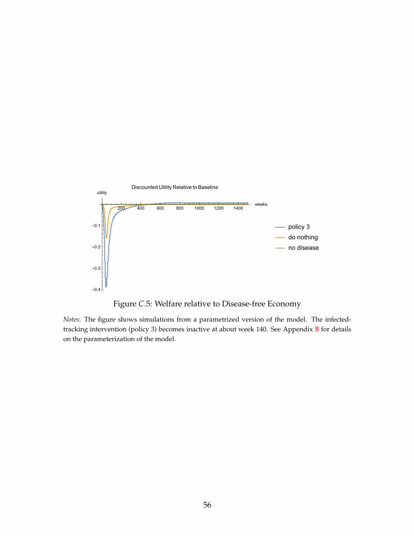
200 400 600 800 1000 1200 1400weeks
-0.4
-0.3
-0.2
-0.1
utilityDiscountedUtility Relative to Baseline
policy 3
do nothing
no disease
Figure C.5: Welfare relative to Disease-free Economy
Notes: The figure shows simulations from a parametrized version of the model. The infected-tracking intervention (policy 3) becomes inactive at about week 140. See Appendix B for detailson the parameterization of the model.
56