MARKET POWER IN THE SPANISH BANKING INDUSTRY A study …

IESE Business School-University of Navarra - 1

MARKET POWER IN THE SPANISH BANKING INDUSTRY

A study of the term deposits market

Jordi Gual

Joan E. Ricart

IESE Business School – University of Navarra Av. Pearson, 21 – 08034 Barcelona, Spain. Phone: (+34) 93 253 42 00 Fax: (+34) 93 253 43 43 Camino del Cerro del Águila, 3 (Ctra. de Castilla, km 5,180) – 28023 Madrid, Spain. Phone: (+34) 91 357 08 09 Fax: (+34) 91 357 29 13 Copyright © 1988 IESE Business School.

Working PaperWP-151 November, 1988 Rev. May 1989

IESE Business School-University of Navarra

MARKET POWER IN THE

SPANISH BANKING INDUSTRY

A Study of the Term Deposits Market

Jordi Gual1

Joan E. Ricart2

Abstract In this paper we study the possibility that the high profitability of the Spanish banking sector is explained by the presence of market power. This market power can arise both in the relation of the sector with its clients (borrowers) and with its suppliers; the people willing to hold bank deposits. The analysis refers to part of this second market where a priori the position of the industry seems to be dominant relative to suppliers. In particular, we study the degree of competition in the market for term deposits, where the atomization of suppliers is stronger.

The analysis in this paper deals directly with the problem of estimating conduct parameters for the industry. We construct a theoretical model of competition in the industry where the presence of market power can be detected due to the liberalization process that has characterized the industry in the last few years.

The paper shows that successive interest rate deregulations produce a rotation in the supply curve. This rotation allows us to distinguish the perceived demand with perfect competition behaviour from that when market power is present. We can therefore test the null hypothesis that the conduct of deposit institutions is analogous to that of perfect competition. At the level of aggregation we have worked, and with the chosen specification, it is not possible to reject the null hypothesis of perfect competition.

NOTE: This project has been funded by the Fundación FIES of the Confederación Española de Cajas de Ahorro (C.E.C.A.). This support is gratefully acknowledged. Comments from Professors R. Caminal, V. Salas, X. Vives and participants at the XV EARIE Annual Conference have been very helpful.

1 Professor of Economics, IESE 2 Professor of Strategic Management, IESE

IESE Business School-University of Navarra

MARKET POWER IN THE SPANISH BANKING INDUSTRY

A Study of the Term Deposits Market

Introduction In this paper we study the possibility that the high profitability of the Spanish banking sector is explained by the presence of market power. This market power can arise both in the relation of the sector with its clients (borrowers), as well as with its suppliers; the people willing to hold bank deposits. The analysis refers to this second market where a priori the position of the industry seems to be dominant relative to suppliers. In particular, we study the degree of competition in the market for term deposits, where the atomization of suppliers is stronger.

By “market power” we understand the ability of a group of agents in a market (in our case the institutions demanding funds), to extract rents from other market participants by way of an implicit or explicit decrease in the degree of competition in the industry. It is well known that this dominant position translates into prices and quantities that diverge from the competitive ones. In the time deposits market this would imply interest rates below competitive rates and an amount of funds which is also below what we would obtain in an efficient market. Usually, this market imperfection implies extraordinary rents or profits that could explain the abnormally high profitability of the industry relative to the rest of the economy.

This classical concept of market power has been traditionally hard to measure in empirical studies of industrial economics. In general, it has been studied indirectly, by means of concentration analysis and other structural variables of the industry. In the Spanish banking sector concentration has increased significantly in the last few years. According to the classical industrial organization paradigm, this increase in concentration could be an indication of increased market power in the industry.

The analysis in this paper directly deals with the problem of estimating conduct parameters for the industry.1 We construct a theoretical model of competition in the industry where the

1 This line of research has been actively promoted in recent years. A volume with some of the more relevant papers has been prepared by Bresnahan and Schmalensee (1987).

2 - IESE Business School-University of Navarra

presence of market power can be detected due to the process of liberalization that has characterized the industry in the last few years.

The second section develops the theoretical model. This model considers a simple deposits-to-loans transformation function. Banks face a deposit supply function and try to maximize profits by choosing as strategic variable the desired quantity of deposits. The supply function will give us the market price given the aggregate level of deposits and other variables. From this model and the corresponding optimization conditions we establish an econometric model for estimation.

Section 3 presents the econometric model. In general these models have an identification problem that might prevent the estimation of the market power parameter. However, in our application to the Spanish banking system, the successive interest rate liberalizations produce a rotation of the supply curve that allows identification. Section 3 describes the identification problems and their solution, the econometric model to be estimated and the database.

Section 4 presents the results. We empirically test the rotation of the supply curve, which validates the opportunity of this methodology. The test on the conduct parameter does not allow us to reject the null hypothesis of perfect competition.

Section 5 presents the conclusions as well as possible extensions of this work. As we have indicated, we cannot reject the null hypothesis of perfect competition in the market for term deposits. This conclusion should probably be checked with better information to ensure its robustness. We would conclude for the moment that the high profitability of the industry must be due to sources other than the implicit or explicit exercise of market power. This industry might show a certain extent of contestability and, as a consequence, firms might behave competitively despite high concentration.

It is important to remark that this paper studies only the behaviour of firms in the specific market for time deposits. This market is characterized by the presence of a large number of substitute products, both private and public, and this could explain the results that we obtain. Moreover, not rejecting the hypothesis of competition in this market does not have implications about the behaviour of financial institutions in the other markets where they operate.

The Theoretical Model We consider financial institutions as firms manufacturing a final good – loans – using deposits as inputs. Bank liabilities are obtained by paying interest r.

In a competitive market, payments for time deposits should equal the value of the marginal product obtained with these deposits. The existence of market power creates a gap between these values so that in equilibrium the value of marginal product exceeds the interest rate on deposits.


The market equilibrium can be described by the deposit supply function and the deposit demand relation by banking firms.2

We specify the following (inverse) supply function

r=f(D,X1); f1>O (1)

where subindices denote partial derivatives, D is the sum of term deposits, r is the interest rate on deposits and X1 is a vector of exogenous variables comprising other determinants of the supply of time deposits. In particular, X1 includes S, a measure of the aggregate banking services supplied in the market.3

The demand relations are obtained from the first order conditions (FOC) of the maximization problems faced by banking institutions. For a monopsony, the problem is the following:

maxD R(L,X3) - rD - C(D,X2)

subject to the following restrictions:

r=f(D,X1)

L=τD

L=V+C

where L are loans (to the public C, or private sector Y), C(D,X2) are total operating costs that depend on the level of D but also on other determinants X2, and R is the total revenue function, with total loans and other exogenous variables X3 as arguments. The constant ti would be 1 minus the reserve coefficient if we were considering all banking deposits. Thus, we would be assuming a very simple transformation from deposits to loans. The use of this model for the term deposits market assumes that there is a stable relationship between time deposits and other liabilities, in particular checking accounts.

We further assume that R and C are differentiable and that R1>0, R11<0 and C1>0. That is, R is strictly increasing and concave,4 and C is strictly increasing in D.

The first-order condition is now:

τR1= f + C1 Df1 (2)

This condition shows that the value of the marginal product must equal the marginal cost of capturing an additional unit of liabilities, whether this additional cost is financial or operational. We assume that the second order condition for a maximum is satisfied.

2 Note that we do not follow here the traditional notation that is used in monetary and financial economics where individuals demand time deposits. From an industrial organization perspective, where the objective is to study the degree of competition in the market for time deposits, it seems more appropriate to use the supply function notation. 3 Since the supply of bank deposits depends on S, one could add this variable to the range of strategic variables available to financial institutions (see Fanjul and Maravall, 1985). However, this approach would require a model with product differentiation. A preliminary version of this paper (see Ballarín et al., 1988, chapter 6) analyzed the case of homogeneous goods but the poor results indicated the presence either of specification errors or of errors of measurement of the S variable. For this reason those results are not reported here. 4 We do not attempt to explicitly model the loan market. However, the assumptions about the revenue function are compatible with some degree of market power in that market.


Of course, monopsony corresponds to an extreme market structure, where the firm enjoys complete control over the choice of price. We consider next the possibility of intermediate market structures that might arise if several firms are in the market for term deposits. We denote these firms with the subindex i, i=1,…, n.

Firms now face a different maximization problem. Note that D=∑iDi, so that the firm faces a residual supply curve depending on the strategies followed by its rivals.

The equilibrium in oligopsony models of this kind depends on the solution concept that is used. From an empirical perspective a possible methodology is to parameterize the different solutions to be able to capture econometrically the degree of competition or collusion in the market. In this work we use the conjectural variation concept to include different solutions to the oligopoly model in a single analytical expression. However, it is worth emphasizing that the use of this concept is purely instrumental, because an equivalent specification would arise with a much less structural approach where expected "reactions" are not explicitly considered, but rather we parameterize the residual demand (or supply in the case of oligopsonists) perceived by firms (see in this regard Bresnahan, 1987).

When we add the conjectural variations concept, the equation system that shows market equilibrium changes substantially. Of course, there is now a multiplicity of competitors and they consider that changes in their strategies may lead to changes in their rivals' strategies. The maximization problem for firm i is then the following:

maxD R(Li) - rDi - C(Di)

subject to the same restrictions.

The first order conditions will be:

τR1 = f + C1 + Dif1 (∂D/∂Di) i=1,...,n. (2b)

where ∂ indicates partial derivative and the terms in parenthesis capture firms' conjectures about their rivals' reactions to changes in their own deposit-seeking activities (∂D/∂Di).5 An alternative notation would be:

(∂D/∂Di)= 1 + ∑j≠i(∂Dj/∂Di)

We assume that these conjectures are parameters and equal for all firms. Note that 2b encompasses some well-known solution concepts for oligopoly games. If (∂Dj/∂Di) = 0, for all j,i; we have a Cournot equilibrium. If, alternatively, (∂Dj/∂Di)=-1/(n-1), we will have a competitive market. Some collusive equilibria can also be described in this context. For example, if marginal costs are constant and equal (∂Dj/∂Di)=1 will correspond to an equilibrium with perfect collusion where firms assume that they can alter market price but not their share of the market. Finally, if marginal costs are not equal, market-share collusion can be obtained with (∂Dj/∂Di)=Dj/Di under certain conditions (Dixit, 1986).

5 The conjectural variations model is like a reduced form of a dynamic model that is not fully specified. Strictly speaking, in our model firms are engaged in a simultaneous game where it makes no sense to talk about "expected" reactions of rival firms.


System 2b may be rewritten as follows for the whole industry:

τR1= f + C1 + θDf1 (2c)

In this system, equation 2 has been transformed introducing the parameter conduct θ that reflects the degree of competition in the market for term deposits through quantity competition.

Equation 2 transforms into equation 2c showing that the marginal financial cost perceived by firms depends on their rivals' expected conduct. Of course, when θ=0 we obtain the condition for perfect competition. When θ=1 we will have Cournot equilibrium (monopsony if there is one firm) and θ >1 will correspond to some sort of collusive equilibria.

Note that equation 2c is equivalent to the system 2b with some additional assumptions since the second system refers to the whole industry.

When data are not available at the firm level, market power analysis must be undertaken estimating the system 1-2c, but then the interpretation of the estimates of θ must be cautious. If market power is present, the shift from 2b to 2c is not possible unless all firms have the same constant marginal costs.6

In general, firms will have different marginal costs at an oligopolistic equilibrium and the interpretation of 2c is then unclear7 (Bresnahan, 1987). Following Cowling and Waterson (1976), under these circumstances the conduct parameters must be interpreted as some sort of weighted average for the industry. Finally, note that if in fact there is no market power, the interpretation of 1-2c is straightforward since in this case the aggregate marginal cost curve is unique.

The Econometric Model

1. Identification Problems in the Econometric Estimation of Market Power

The n equation system (2b), together with (1) determines the quantities (Di) and the equilibrium interest rate in the time deposits market. At the same time, they provide a simultaneous equation system that can be estimated econometrically. If we only have aggregate data it is possible to estimate the system (1) - (2c) even though that implies that there are some problems with the interpretation. However, this is the approach used in this paper given the data limitations.

In principle the supply equation and the demand relation may be identified in the traditional fashion if the exclusion restrictions are satisfied. That is, in an empirical specification the supply function must include a set of exogenous variables, X1, that includes those supply determinants that do not affect demand. Similarly, (2) includes exogenous variables, X3, that change only the value of marginal product and variables X2, that shift the operating marginal cost function.

6 It is also possible when we have a cartel that perfectly allocates production between its members so that marginal costs are equal for all members and therefore equal to industry marginal costs. 7 If firms have different marginal costs the aggregate marginal cost curve depends on the market share of each firm in the resulting equilibrium.


Even though the equation system is identified, that is we can distinguish one equation from each other empirically, this does not imply that a priori we are able to estimate all parameters of interest. In particular, Bresnahan (1982) and Lau (1982) have shown that in an oligopoly model the market power parameter is not identified in general.

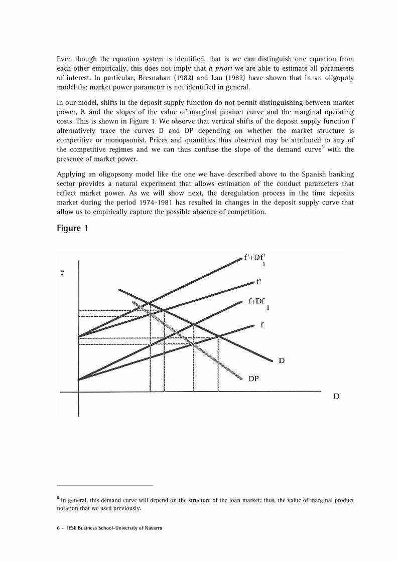
In our model, shifts in the deposit supply function do not permit distinguishing between market power, θ, and the slopes of the value of marginal product curve and the marginal operating costs. This is shown in Figure 1. We observe that vertical shifts of the deposit supply function f alternatively trace the curves D and DP depending on whether the market structure is competitive or monopsonist. Prices and quantities thus observed may be attributed to any of the competitive regimes and we can thus confuse the slope of the demand curve8 with the presence of market power.

Applying an oligopsony model like the one we have described above to the Spanish banking sector provides a natural experiment that allows estimation of the conduct parameters that reflect market power. As we will show next, the deregulation process in the time deposits market during the period 1974-1981 has resulted in changes in the deposit supply curve that allow us to empirically capture the possible absence of competition.

Figure 1

8 In general, this demand curve will depend on the structure of the loan market; thus, the value of marginal product notation that we used previously.


2. Interest Rates Deregulation and Changes in the Term Deposits Supply Function

The aggregate supply curve for time deposits is obtained as a horizontal sum of three different kinds of supply functions. We consider three classes of deposits corresponding to terms of six months, D6; between one and two years, Di; and more than two years D2. The direct supply functions are assumed to be linear and this allows us to simply incorporate substitutability between deposits. These functions are:

D1 = A1 + d1r1 – f1r2 – f1r6

D2 = A2 + d2r2 - f2r1 - f2r6

D6 = A6 + d6r6 - f6r1 - f6r2

where the corresponding interest rates are r1,r2 y r6 and where we assume that Ak>0, and dk>2fk, k=1,2 and 6.

However, it is assumed that in an equilibrium situation the three interest rates are linked by a linear relation because of a liquidity premium that implies higher interest rates for longer terms. This relation can be written as follows:

r2=τ0 + τ 1r1

r1=τ2 + r3r6; τ0, τ1, τ2, τ3,> O.

Thus, the aggregate deposits supply can be written as a function of a single interest rate

D = α0 + α1r1 (4)

where D=D1+D2+D6 and the parameters keep the following relationships:

α0 = A1+A2+A6 + τ0 (d2-f1-f6) -(τ2/τ3)(d6-f2-f1)

α1 = τ1(d2-f1-f6) + (1/τ3)(d6-f2-f1) + (d1-f2-f6)

Under regulatory conditions this supply curve changes. Suppose the restriction is the following: r6 ≤*. When the constraint is binding, the aggregate supply function becomes:

D = α0 + α1’r (5)

where:

α0’ = A1+A2+A6 + τ0(d2-f1-f6) + r*(d6-f2-f1)

α0’ = τ1(d2-f1-f6)+(d1-f2-f6)

so that α0’>α0 and α1’<α1.

This shows that interest rate deregulation results in a change in the supply function modifying both the slope that goes up and the level that falls. As we will see, it is this rotation of the supply curve that allows us to econometrically identify the parameter θ.

Changes in the supply function may be incorporated for the empirical analysis using a dummy variable with value O for periods previous to the deregulation and 1 for periods after. For the Spanish financial sector, since deregulation takes place in two stages, we introduce additional


dummy variables. Thus, for the 1974-1984 period we can specify the following aggregate supply function:

D = α1 + α2Z1 + α3rZ1 + α4Z2 + α5rZ2 + α6X1 (6)

where the value of Z1 is 1 from the fourth quarter of 1977 (deregulation of interest rates between one and two years) and Z2 is 1 from the third quarter of 1981 (deregulation of interest rates between six months and one year). Note that the interest rate does not belong to the equation in the first period. This makes sense because the interest rate chosen for the empirical analysis is the one corresponding to time deposits between one and two years, that were deregulated in September 1977. Similarly, we have included the variable X1 that includes other factors that shift the aggregate supply function.

To show that the problem of identifying θ and μ is solved by specifying equation (5) we have to detail the functional form for the operating costs and revenue functions.

We will assume that operating total costs are quadratic:

C(D,X2) = constant + β1D + (1/2) β2D2 + β3X2D

and the following total revenue function:

R(L,X3) = R(V+C)= constant + Γ0V - (1/2) Γ1v2+ rBC + Γ2X3L

where V= τD - C and the parameters β1, β2, Γ0 and Γ1 are positive; V and C indicate financing to private and public sector; the interest rate for public sector credit is rB and we have introduced X2 and X3, related to the operational marginal costs and marginal revenue curves.

The first order condition is now:

τΓ – τ2 Γ1D + τΓ1C+m + τΓ2X3 = r + (α3Z1+α5Z2) - 1θD + β1 + β2D+ β3X2 (6)

If we define D*. (α3Z1+α5Z2)-1D and reorganize (6), we obtain the following system, where (5) is added again:

D = α1 + α2Z1 + α3rZ1 + α4Z2 + α5rZ2 + α6S + α7X0 (5)

(β2 + τ2Γ1)D = (τΓ0 – β1) - θD* - r + τΓ1C + τΓ2X3 – β3X2 (7)

In this system the market power parameter is identified since D and D* are not perfectly correlated.

The role of Z1 and Z2 in the identification of the parameters of interest is clear. If Z1 = 1 and Z2 = O for all observations, we have D* = D/α3 and the equation system becomes:

D = (α1 + α2) + α3r + α6X1 (5')

r = (τΓ0 – β1) - (β2 + τ2Γ1+ θ/α3)D + τΓ1C + τΓ2X3 – β3X2 (7')

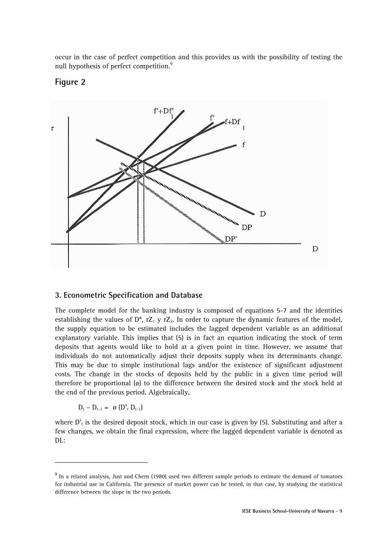
The conduct variable θ cannot be distinguished from the slope of the marginal revenue function or the slope of the operating marginal costs. This is illustrated in Figure 2 where we can see how the rotation of f produces a rotation in DP (perceived demand), which is the demand curve one obtains from the observation of prevailing prices and quantities. This rotation does not


occur in the case of perfect competition and this provides us with the possibility of testing the null hypothesis of perfect competition.9

Figure 2

3. Econometric Specification and Database

The complete model for the banking industry is composed of equations 5-7 and the identities establishing the values of D*, rZ1 y rZ2. In order to capture the dynamic features of the model, the supply equation to be estimated includes the lagged dependent variable as an additional explanatory variable. This implies that (5) is in fact an equation indicating the stock of term deposits that agents would like to hold at a given point in time. However, we assume that individuals do not automatically adjust their deposits supply when its determinants change. This may be due to simple institutional lags and/or the existence of significant adjustment costs. The change in the stocks of deposits held by the public in a given time period will therefore be proportional (ø) to the difference between the desired stock and the stock held at the end of the previous period. Algebraically,

Dt – Dt-1 = ø (Dst Dt-1)

where Dst is the desired deposit stock, which in our case is given by (5). Substituting and after a

few changes, we obtain the final expression, where the lagged dependent variable is denoted as DL:

9 In a related analysis, Just and Chern (1980) used two different sample periods to estimate the demand of tomatoes for industrial use in California. The presence of market power can be tested, in that case, by studying the statistical difference between the slope in the two periods.


D = øα1 + øα2Z1 + øα3rZ1 + øα4Z2 + øα5rZ2 + øα6X1 + (1-ø) DL (6b)

With respect to the demand relation, it is necessary to point out that it is estimated only for the period 1977(III)-1984(IV) because the variable D* is not defined for the period 1974(I)-1977(II). However, the supply equation has been estimated for the whole period because the additional information increases the precision of the estimators used in the calculation of D*. Note that although D* is a nonlinear function of D, Z, and the parameters α3 and α3, the 2SLS (two-stage least squares) estimation is possible because no instrument is necessary for D* in the first equation.

All equations have an error term which we assume to be additive. The assumptions on the error terms are the usual ones. They are independently and identically distributed random variables with no serial correlation.

As for the exogenous variables included in the model, those that one should include a priori are detailed next.

The variable X1 includes determinants of the aggregate supply of deposits like aggregate disposable income, the level of aggregate banking services and the returns on alternative financial assets. The variables (X3) that shift the marginal revenue function include the economic activity level and investment demand for capital goods. Shifts of the operating marginal cost functions (X2) are captured by changes in variable (labor) costs and shifts in the operating marginal cost function corresponding to technological improvements. The appendix shows the specific variables that have been selected for the empirical analysis.

The final specification includes variables P, Gross Domestic Product and S, number of branches per employed person, as components of X1; F, Gross Fixed Capital Formation as an element of X3

10 and t, a trend variable, as an element of X2. The system of equations to be estimated is then:

D = øα1 + øα2Z1 + øα3rZ1 + øα4Z2 + øα5rZ2 + øα6S + øα6S + øα7P (1-ø) DL (8)

(β2 + τ2Γ1)D = (τΓ0 - β1) r + θD*+ τΓ1C + τΓ2F – β3t (9)

The appropriate estimation method at first instance seems to be two-stage least squares (2SLS). This is a simple method that solves the simultaneity problem that leads to inconsistent estimates if we use ordinary least squares (OLS). With 2SLS the system is estimated equation by equation. It is therefore a limited information system that does not use the a priori acknowledge of cross equation restrictions that one may have, but it is the appropriate method for industry-wide data.

Results The results from the estimation of (8) and (9) using OLS and 2SLS are presented in Table 1. Some considerations are necessary before we analyze these results. The supply equation does not include two exogenous variables Ro and Rd that were intended to capture the evolution of alternative investment opportunities. These variables are strongly correlated with the interest

10 The variable P, GDP, is not in the equation because its inclusion perversely affects the signs of the other parameters. Also, the labor cost variable, W, has been omitted because it was not statistically significant.


rate and its inclusion in the equation gives rise to (non-significant) parameters with the wrong sign and biased estimation of the interest-rate coefficient.

The supply equation presents serial correlation. When a retarded dependent variable was included, the presence of autocorrelation of degree 1 was tested with Durbin's H test.11 The final estimation has been done using the 2SLS method even though OLS results are also reported. In particular, given the presence of the lagged endogenous variable in the first equation, the serial autocorrelation has been corrected with the Prais-Winsten method, using the two stage estimator suggested by Hatanaka (1974).

The estimated supply equation seems quite correct. One can check empirically that the successive interest rate liberalizations produce a rotation of the supply curve in the direction of decreasing intercept and substantial increase in the slope. Clearly, we cannot reject the null hypothesis that the interest rate liberalization has produced a rotation in the supply curve. We observe a statistically significant fall in the intersect, both for 1977 and 1981, together with an increase in the slope for both periods. This is a central result since otherwise it would not be possible to identify the interesting parameters in the model.

The estimation of the coefficient corresponding to the retarded dependent variable, DL, is (1-ø) = .9057. This implies that only 9.43% of the desired change in the stock of deposits takes place in the same period. This proportion is very low, but one has to consider that the collinearity between the variables P and DL can reduce the precision of the estimation.

The results for the demand relation shown in Table 1 provide a good regression fit and all the explanatory variables have the right sign.

We can contrast the null hypothesis of perfect competition with a simple test to check whether the parameter corresponding to D* is significantly different from zero. This test does not allow us to reject the null hypothesis of perfect competition, because the value of the statistic is -1.432. This value is clearly not significant even at a 90% confidence level. With a more structural interpretation of the model, we could calculate a point estimate for π as the ratio between the parameters of D* and r. This estimate is 0.00577, so close to zero that a formal test to contrast the null hypothesis, H0: θ=0, does not seem necessary.

Although the model does not attempt to estimate the parameters of the cost function, it is possible to derive a point estimate of β2 from the point estimates of 1/(β2 + τ2Γ1), τΓ1/(β2 + τ2Γ1) and the sample value of τ. This point estimate is .002831, extremely close to zero -constant returns to scale- although the precision of the estimate is so low that no general conclusions can be drawn.12

11 The H Durbin test is expressed as H=ρ(T/(1-TV(1-ø)))½ where T is the number of observations, p the estimated serial correlation of degree one and V(1-ø) the estimated variance of the lagged variable (see Maddala, (1977), p. 372). In our case, , and we can reject the null hypothesis of no serial correlation with a 95.66% probability. 12 In this regard, it is clear that we could estimate (8) and (9) together with the factor demand equations. This would, of course, require further information but one could attain a more efficient estimation (in particular of cost parameters), and an opportunity to test the specification of the model thanks to cross-equation restrictions.


Table 1 OLS and BLS estimation of the model (8-9)

variable supply (OLS) supply (2SLS) demand (OLS) demand (2SLS)

constant 280.441 280.075 -836.312 -167.754 (149.3) (143.9) (494.0) (577.3)

Z1 -532.84 -531.214 -- -- (277.2) (266.5)

rZ1 52.868 52.7283 -- -- (26.70) (25.71)

Z2 -2288.85 -2295.18 -- -- (927.5) (890.9) rZ2 179.553 180.048 -- -- (72.54) (69.98) S -.575436 -.574548 -- -- (.2436) (-.2362) P .376669 .375943 -- -- (.1425) (.1402) DL .9054 .905703 -- - (.05558) (.297145) r -- -- -162.91 -258.289 (67.88) (80.97) D* -- -- -1.91972 -1.49074 (1.083) (1.041) t -- -- 215.529 238.323 (35.42) (34.96) C -- .168168 .104137 (.0572) (.06306) F -- -- 2.12825 1.98041 (1.112) (1.034) Adjusted R2 .99958 .99957 .99757 .99736 ρ .291266 .297145 .38402 .30664 DW 1.4175 1.4186 1.2326 1.3867

The figures in parenthesis are standard errors. p is the estimated serial correlation coefficient and DW is the corresponding Durbin-Watson coefficient. See the appendix for variable definitions.

Conclusions The analysis presented in this paper is tentative in nature with emphasis on a methodology for estimating market power in the Spanish banking sector. The paper has shown the theoretical possibility of doing a rigorous analysis of this point. The successive interest rate deregulations produce a rotation in the supply curve as we have demonstrated both theoretically and empirically. This rotation allows us to distinguish the perceived demand with perfect competition behaviour from that when market power is present. This distinction allows us to test the null hypothesis that the conduct of deposit institutions is analogous to that of perfect competition.

Our results should be considered partial and preliminary. At the level of aggregation we have worked, and with the chosen specification, it is not possible to reject the null hypothesis of perfect competition. We have shown that our methodology is useful, and a more disaggregated


future analysis can confirm or modify this initial conclusion. We have seen that such an analysis is possible and that the market power parameter can be estimated. This work has shown that it is necessary to have access to larger and better information to perform this task.

It is important, nonetheless, to stress two points. First, the market we have considered -the term deposits market- is a market with clear substitute products, both in the form of public debt and private assets. This might justify a higher degree of rivalry in that market. Second, our analysis has no implications about the general behaviour of financial firms. High profitability could arise from asset operations, commissions on services or other liability operations. Finally, one should keep in mind that observed profitability corresponds to accounting measures that need not reflect truly economic profits.

The possible improvements of this paper can be summarized in two alternatives. On the one hand, it is important to work with data at the level of bank groups, to distinguish between savings institutions and commercial banks, as well as between small and large institutions. This level of detail will introduce new restrictions into the model (relating parameters in different equations) and will allow us to statistically test the fit of the model to the data. Furthermore, we could incorporate different behaviour for different institutions (for instance, the 7 large banks and the main savings institutions acting as leaders).

A second line of improvement has to do with the quality of the data being used. The provision of services might be an important competitive factor in the industry. But the variable we have used does not behave adequately; therefore, we have been unable to correctly analyze its impact in the sector. An interesting research area may be the search for an adequate variable to be used to take into account the effort being made by financial institutions to provide services in order to attract more deposits.

Similarly, one can improve the cost variables. The use of a trend as a proxy for technological improvements is not a convincing approximation. Furthermore, it is suspicious that labor costs are not a significant variable in the estimation.


Appendix Definition of Variables (Quarterly data for the 1974-1984 period. Private Banks as defined by the Bank of Spain)

Exogenous Variables

Deposits Supply Function:

Y: GDP at market prices. Quarterly adjustment by R. Sanz using the quarterly industrial production index published by the MINER (billions of current ptas.13) (Bank of Spain).

R0: Internal return on private securities (in percent) (Bank of Spain).

Rd: Average internal returns on Government debt with maturity of two years or longer (in percent) (Bank of Spain).14

S: Number of branches per employed population (branches per million employed individuals) (Bank of Spain and INE).

Marginal Revenue Function:

Y: (see previous comments).

F: Gross Fixed Capital Formation15 (billions of current ptas.) (INE).

C: Public Sector Borrowing Requirements (billions of current ptas.) (Bank of Spain).

Operating Marginal Cost Functions:

W: Monthly Average Earnings by worker in financial institutions (simple quarterly averages in current pesetas) (INE)16.

t: Trend variable with value 1 for observation 1974-I and 44 for observation 1984-IV.

13 Data in nominal terms have been obtained using the GNP deflator (base 1970), adjusted quarterly using the seasonally adjusted non-food Consumer Price Index. Both series are published by the Bank of Spain. The quarterly adjustment is performed following a technique suggested by Fernández (1981). We use an indicator series that is available on a quarterly basis and that has an annual behavior similar to the series that we want to adjust. GLS is used to estimate a model where the variable that is to be adjusted is a function of the indicator variable and where we impose the restriction that the new quarterly adjusted variable has to add to the yearly variable. This procedure avoids jumps in the new series since the adjusted variable is constructed using the estimated regression coefficient and the indicator, and the assignment of residuals derives from the estimation procedure (we appreciate comments by Fernando Alvarez (INE) on the issue of quarterly adjustments). 14 For the 1974-1977 period this series is interpolated using the Ro series. The Government debt interest rate series for the 1974-1/1977-IV period is obtained by a procedure suggested by Mauleón (1987). A regression for the 1978-I/1984-IV period is estimated where the change in the Government debt interest rate is explained by the change in the return on private securities both contemporaneous and lagged one period. The regression coefficients are (.44251) and (-1.65545). The resulting equation is used to interpolate the government debt series for the first period of the sample. 15 Quarterly adjusted series using as an indicator die capital goods investment series (index numbers, base year 1980). This series is produced by INE using the Industrial Production Index and capital goods import and export indices. Seasonally adjusted series (INE). 16 This series corresponds to ordinary and extraordinary payments, including overtime payments, in the financial institutions industry. For 1974-1978, it is a yearly series, and the quarterly adjustment was done using as indicator simple averages of the monthly salary per worker.


Appendix (continued)

Dummy Variables:

Z1 Dummy variable with value O between 1974-I and 1977-III and 1 thereafter.

Z2 Dummy variable with value O between 1974-I and 1981-II and 1 thereafter.

Endogenous Variables:

r: Interest rate. Time deposits between one and two years (in percent) (Bank of Spain).

D: Time Deposits and Deposit Certificates for more than 6 months (Billions of current pesetas) (Bank of Spain).


References Ballarín, E., Gual, J., and J. E. Ricart (1988), “Rentabilidad y Competitividad en el Sector Bancario Español. Un Estudio sobre la Distribución de Servicios Financieros en España," IESE, Universidad de Navarra, mimeo, February.

Bresnahan, T. (1982), “The Oligopoly Solution Concept is identified," Economic Letters, 10, 1, pp. 87-92.

Bresnahan, T. (1987), “Empirical Studies of Industries with Market Power," forthcomming in Handbook of Industrial Organization, ed. R. Schmalensee y R. Willig, North Holland.

Bresnahan, T. and R. Schmalensee (1987), “The Empirical Renaissance in Industrial Economics,” Basil Blackwell, Oxford.

Cowling, K. and M. Waterson (1976), “Price Cost Margins and Market Structure," Economica, 43, 171, pp. 267-274.

Dixit, A. (1986), “Comparative Statics of Oligopoly," International Economic Review, 27, 1.

Fanjul, O. and A. Maravall (1985), “La eficiencia del sistema bancario español,” Alianza Universidad, Madrid.

Fernández, R. B. (1981), “A Methodological Note on the Estimation of Time Series," The Review of Economics and Statistics, 63, 3, August, pp. 471-476.

Hatanaka, M. (1974), “An Efficient Two-Step Estimator for the Dynamic Adjustment Model with Autocorrelated Errors," Journal of Econometrics, pp. 199-220.

Just, R. and W. Chern (1980), “Tomatoes, Technology and Oligopsony," Bell Journal of Economics, 11, 2:584-602.

Lau, L. (1982), “On Identifying the Degree of Competitiveness from Industry Price and Output Data," Economics Letters, 10, 1-2, pp. 93-99.

Maddala, G. S. (1977), “Econometrics,” MacGraw Hill, New York.

Mauleón, I. (1987), “Determinantes y perspectivas de los tipos de interés," Papeles de Economía Española, 32, pp. 79-92.

Documents

MARKET POWER IN THE SPANISH BANKING INDUSTRY A study …