1

Market Power and Transmission Congestion in the Italian Electricity Market

Simona Bigerna, Carlo Andrea Bollino and Paolo Polinori*

ABSTRACT

Analysis of market power in electricity markets is relevant for understanding the competitive development of the

industry’s restructuring and liberalization process, but in the existing literature, there is not an adequate consideration of

line transmission congestion. The aim of this paper is to propose a new approach to measuring market power in the

Italian Power Exchange (IPEX), explicitly considering transmission line congestion. We construct a new measure of the

residual demand curve to disentangle unilateral market power from congestion rent for the main Italian generators

during the period April 2004 to December 2007. In Italy, this period was one of stable transmission network structure.

Following the approach of Wolak (2003, 2009), we measure the unilateral market power with the Lerner index (LI),

computed as the inverse of the residual demand elasticity. In conclusion, the correct modeling of the residual demand

curve including transmission congestions enables us to compute the zonal LI and therefore more accurately measure the

market power when congestion occurs. Our results show that various generators exercise market power only in specific

zones. These findings provide deeper understanding of market outcomes in the presence of congestion, suggesting

appropriate policy directions for market surveillance and competition regulation.

Keywords: Market power, Residual demand, Transmission congestion, Zonal Lerner index

*Department of Economics - University of Perugia, Via Pascoli 20, 06123, Perugia, Italy. Corresponding author: Paolo Polinori, E-mail: paolo.polinori@unipg.it.

2

I. INTRODUCTION

Electricity market reform is nearly two decades old in most industrialized countries. These

reforms followed the pioneering revolutions that occurred at the beginning of the 1990s in the UK

(1990), Norway (1991) and the USA (1992). In particular, there has been a progressive fading of

monopolies and administered prices in Europe since Directive 96/92/EC. Market mechanisms have

been introduced progressively, but there is still doubt that electricity markets have become

competitive. The prior studies have analyzed the exercise of unilateral market power by generators

by utilizing empirical evidence that demonstrates that markets are oligopolistic and primarily

employs bid data (Borenstein et al. 2002, Wolak 2003, 2009, Sweeting 2007, Bollino and Polinori

2008, McRae and Wolak 2009, Bosco et al. 2012). However, the analysis in this literature has been

limited to those cases in which the transmission network is similar to a single bus bar, i.e., when

there is only one hourly market.

The relationship between congestion and market power in electricity spot markets has been

analyzed primarily on a theoretical basis (Cho and Kim 2007). Recently, Lee et al. (2011) have

proposed a new approach to measure market power in presence of transmission constraint, while

Karthikeyan et al. (2013) provided a comprehensive review of market power. The benefits of

transmission expansion are well-described in Wolak (2012), but to date, there is no empirical

analysis of the effect of line congestion on zonal price differentials using bid data1.

The aim of this paper is to measure market power when different zonal prices arise in an

electricity market as a result of congestion. To this end, we propose a novel approach to measuring

market power empirically by explicitly disentangling this from the impact of network congestion on

market structure, equilibrium prices, and operators behavior. In detail, we provide the correct

formula for calculating the zonal Lerner Index (LI), by explicitly considering the transmission

congestion problem. We propose to modify the residual demand computation (as originally

1 However, Shukla and Thampy (2011) investigated market structure and competitiveness in India, taking into account the implications of transmission congestion on competition. More recently, Mirza and Bergland (2012) estimated the non-competitive effects of transmission congestion in Norway. Finally Nappu et al. (2013) analyzed whether market power exercise can cause transmission congestion in interconnected zones.

3

proposed in Wolak 2003, 2009), considering explicitly line congestion and consequently, two

different types of offer bids. The first are offer bids refused by the Transmission System Operator

(TSO)2, even if they are more competitive than the marginal bid. The second are the offer bids

accepted by the TSO, even if they are more expensive than the marginal bid. This approach enables

us to compute a correct measure of zonal market power.

We investigate the initial period (April 2004 - December 2007) of the day-ahead market of the

Italian Power Exchange (IPEX). This period is an interesting one to study, characterized by two

main features: (i) the transmission network structure was relatively stable; (ii) the renewable energy

sources (RES) share was negligible. Indeed the RES boom in Italy started in 2008 to 2009.

Therefore, we study a period of stable generation and transmission network structure, which can be

interesting also for developing electricity markets in other regions of the world. In fact, in countries

such as Argentina, Colombia, Venezuela, Thailand, the Philippines, and Taiwan and most oil

producers, the share of RES in electricity generation is currently approximately 2 or 3% (excluding

hydro). In other words, analysis of the Italian market at an early stage of the liberalization process

can shed light on the critical issues that those countries could face in the future, if they overlook the

congestion issue.

This paper is organized as follows. Section 2 describes the main features of the IPEX and

market segmentation. Section 3 describes the new methodological approach to measure market

power at the zonal level with a transmission congestion and data construction procedure. Section 4

discusses the empirical analysis and results. Section 5 summarizes our primary findings. The

method details and statistical information are provided in the Appendices.

II. THE ITALIAN ELECTRICITY MARKET

The IPEX is one of the last pool markets created in Europe after Directive 96/92/EC for

energy sector liberalization. The IPEX is organized as a day-ahead, adjustment and dispatching 2 In Italy, the TSO was initially GRTN in 2004 and has been TERNA since 2005.

4

resource market, similar to that of other countries (Newbery, 2005), and started operation in April

2004 (Law 79/99, Law 240/04 and other Decrees)3.

We focus on the hourly spot market4, which yields a System Marginal Price (SMP). When

there is congestion, market segmentation arises, and the consequence is that different zonal SMP are

determined. To appreciate the importance of the congestion effect on the market in the period

analyzed, note that there are a total of 32,880 hours and a total of 77,004 market zones and

consequently 77,004 different market equilibrium prices to be considered. The TSO determines

congestion as intended flows in excess of the physical transmission capacity based on supply and

demand bids. Consumers pay a unique SMP on the demand side, which is computed as a weighted

average of the zonal SMP on the supply side.

In the period analyzed, the Italian transmission network characteristics remained unchanged

compared to the pre-liberalization period. Investment in new lines started with a period of delay,

and the network management began dispatching intermittent renewable energy sources in 2008.

Therefore, in this period, market liberalization developed under the constraint of the old network

arrangement, generating line congestion due to the physical line capacity limits coupled with an

approximately stable generation capacity. The main features of the market in this period can be

summarized as follows. (i) In 2004, only suppliers participated in the market, and demand was

inelastically represented by the TSO5. (ii) In January 2005, active demand bids entered the market,

and the TSO was able to overrule bids if the total market demand was “too different” from the

independent day-ahead forecasts used for security management. (iii) In January 2005 the Single 3 In the spot market, agents submit supply and demand bids for the 24 hours of the next day. In the adjustment market,

generators and loads submit offers/bids to correct parts of the schedules that cannot be implemented due to technical

constraints. The third market is used by the TSO for procuring congestion-relieving resources and creating adequate

secondary and tertiary control reserve margins. In this market, resources are valued on a pay-as-bid basis.

4 This is a non-compulsory pool market administrated by a Market Operator, in Italian, Gestore del Mercato Elettrico

(GME).

5 For further details on the first year of IPEX activity, see Bollino and Polinori (2008).

5

Buyer, in Italian Acquirente Unico (AU), was empowered to aggregate non-eligible and poor

customer demand6 and was instructed to utilize contracts for differences extensively and to buy into

the market; as a result, market liquidity rose over 60%. (iv) The Italian Energy Authority enacted

several pro-competitive market surveillance mechanisms aimed at discouraging producer quantity

withholding strategies. The Energy Authority also regulates market data disclosure. (v) The RES

has had dispatching priority since 2008, and it started to inject relevant flows into the network with

the new feed-in tariff mechanism. In this period, the generation capacity in Italy has been quite

concentrated and over two-thirds of this capacity is fueled by oil and natural gas (Table 1). ENEL,

the former State-owned monopolist, had a market share of 48-49% in 2004 and of approximately

30% in 2007. The other main generators (newcomers, which have bought capacity from ENEL

according to the liberalization rules) initially had a share of another 25% of production in 2004,

which gradually rose to 33% in 2007.

[Table 1 here]

The hourly demand pattern is typically bimodal, indicating the increasing similarity between

summer and winter peak demand (above 50,000 MW in 2007), but the primary feature has been that

the household and industrial user prices were higher in Italy than in the rest of Europe. Thus, the

IPEX differs from other European electricity markets in terms of prices, market liquidity, fuel mix,

incentive mechanisms and market segmentation or configuration because of congestion problems

(as discussed in detail below). All things considered, the German market appears to be the most

6 In Italy, the AU intermediates the demand for non-eligible customers according to the Government and Regulatory

Authority directives and operates mainly with contracts for differences. Thus, the AU is the main counterpart for market

operators in contracts for differences. The result is that the strike price and, often, the quantity and load profile of the

AU are strongly influenced, if not imposed, by those public authorities.

6

similar to the IPEX. In particular, the prices paid for low voltage usage (e.g., contracts in the 2.5-5

MW range) are similar in Italy and Germany (Bigerna and Polinori 2014).

The Italian market is divided into seven physical national zones (PNZ) (Table 2, Panel 1):

North Italy (N), Center-North Italy (Cn), Center-South Italy (Cs), South Italy (S), Calabria (Cal),

Sicilia (Si, Sicily in English) and Sardegna (Sa, Sardinia in English)7.

[Table 2 here]

When there is congestion, the IPEX is segmented in a variable number of zones (Nz), (1≤ Nz

≤ 7), and we name this configuration the “Nz-market”. Each configuration includes Nz “markets,”

each of which is generally characterized by a different SMP. Obviously, these markets can be

constituted by a single PNZ or by many interconnected PNZs. In the second case, we label

“elementary zone” each PNZ belonging to that market (Table 2, Panel 2). For example, if Nz is

equal to three, then there are several three-market configurations. In one case, the three markets can

be ML, Si and Sa. In this configuration, Si and Sa are both markets and PNZ, but ML is a market

made up by the interconnected elementary zones of N, Cn, Cs and S. In another case, the three-

market configuration can be N, IeNSi and Si, and so on. IPEX segmentation due to congestion

resulted in 77,004 hourly markets in the period considered (Table 3), which yielded an average of

2.34 markets per hour (as there were 32,880 hours in the period).

[Table 3 here]

The hourly number of markets varies throughout the period. One-market (ITA) occurred for

5,989 hours (18.2% of the hours in the period). Five or more markets occurred for only 110 hours

(0.33% of the total). The most common configurations are two- and three-market, which together

7 Given the shape of the country, the first six PNZs are adjacent along the north-south direction, but the Sa is connected

to Cn with a High Voltage Direct Current (HVDC) line.

7

occurred for 23,540 hours (71.59% of the total), and the two most frequent configurations are Si,

MLSa, which occurred for 7,765 hours (23.65% of the total), and Si, Sa, ML, which occurred for

4,260 hours (12.96% of the total). Not surprisingly, the islands are often separated from the rest of

the network: Sa was a separate market for 11,618 hours (35.3% of the total), and Si was a separate

market for 18,889 hours (57.4% of the total). At other times, one of the two main islands is joined

with nearby zones.

We present the annual equilibrium price statistics over the period for various market

configurations, from one-zone to more than four zones (Table 4). In detail, we notice that the hourly

market equilibrium prices are higher when the number of hourly markets is higher; for instance, in

2007, the average price in the one-market configuration was 51.1 EURO/MWh while it was 88.7

EURO/MWh in the four-market configuration. In addition, in this period price trends differed

according to the number of markets. Namely, the average price increased 14% in the one-market

configuration (from 43.5 to 51.1 EURO/MWh), but the average price increased 49.4% (from 57.3 to

88.7 EURO/MWh) in the four-market configuration in the same period (Table 4)8.

[Table 4 here]

We consider the equilibrium prices that result in the most frequent configurations (which

account for 80.4% of the hours) in the whole period, as reported in Table 5. It is noteworthy that

there is wide variability within each market configuration. Price averages range between 54 and

81.9 EURO/MWh in the one- and two-market configuration, but the price reaches 93.2 EURO/MWh

8 More detailed computations are provided in Appendix C. We have tested for average price differentials among

different market configurations, for i,j = 1, 2..5, the Prob (µi- µj < 0). Price is significantly higher in the 2-market vs. 1-

market configuration (Prob = 0.0000; t = - 8.4269, df = 19,119); in the 3- vs. 2-market (Prob = 0.0000; t = - 7.8153, df =

23,538): in 5- vs. 4-market (Prob = 0.043, t = - 2.3707, df = 3,349). The price differential is not significant in the 4- vs.

3-market configuration.

8

when there is a three-market configuration; the prices are always higher in the Southern zones and

in the islands (especially in Si, which records the highest prices), possibly also because of different

fuel mixes. There is also heterogeneity among the hourly market price differentials. In the two-

market configuration, the differential is in the order of 23.7% between Sa and MLSi (66.9 vs. 54.1

EURO/MWh), but it is smaller (10%) between Si and MLSa (66.85 vs. 62.47 EURO/MWh). In the

three-market configuration, this price differential is greater than 20% between Sa and ML and

between Si and N (66.13 vs. 55.39 and 93.22 vs. 75.88 EURO/MWh, respectively).

[Table 5 here]

In summary, our congestion analysis indicates that there is clearly wide hourly market price

variability. Despite this finding, previous studies on the IPEX have not fully analyzed this

variability. Several studies have taken into account only the one-market configuration (Bosco et al.

2012, Perekhodtsev and Baselice 2010), and others have focused on zonal prices without employing

bid data (Gianfreda and Grossi 2012) or utilized bid data for only a short period (Boffa et al. 2010)9.

This motivates our research to carefully measure the effect of the strategic price setting of Italian

generators by explicitly considering the line congestion effect and employing bid data.

III. RESIDUAL DEMAND AND TRANSMISSION CONSTRAINTS

The measurement of firm-level strategies in the IPEX, i.e., the unilateral market power,

requires understanding how each generator formulates its bid strategy to maximize its expected

profit. Among several methods (Karthikeyan et al. 2013), we compute the market power in the

IPEX starting from the consolidated theoretical framework (Wolak 2003, 2009) by utilizing the LI

as shown in detail in Appendix A.

9 Other studies have analyzed the IPEX from various points of view; see among others Petrella and Sapio (2012).

9

In the context of firm interaction on the supply side, the analysis of unilateral market

power entails the computation of the LI based on the inverse elasticity of the residual uncontracted

demand (RD) curve that faces each market participant. This allows us to analyze the hourly

relationship between price and quantity bid by each firm by considering the supply response of all

other firms (Baker 1988). The LI can be interpreted as a measure of the unilateral market power

exercised by firm i in each state. Support for this interpretation is provided by market rules in Italy,

which do not restrict the ability of suppliers to submit bids. Accordingly, suppliers can submit bids

any time before market closure and revise bids freely for the entire daily span as many times as a

producer deems necessary to adjust its production schedule10.

However, when market segmentation occurs due to congestion constraints between two

zones, the equilibrium market price varies, which gives rise to a congestion rent. The price is higher

in the importing zone because, to satisfy local demand, some additional local plants must be

accepted in the merit order instead of less expensive plants from the neighboring zone. Thus, a

measure of market power computed as a mark-up over the marginal cost at such an equilibrium

price is doomed to include such congestion rent. We address the issue of computing the LI

interpreted as a measure of unilateral market power at the zonal levels by considering market

segmentation.

In fact, market segmentation can change the relevant position of the RDh,i curve that each

supplier faces; we want to explicitly take this fact into account when estimating RDh,i, or else there

is a risk of biased results (Wolak 2009). The extant literature has not addressed this issue explicitly.

We tackle this issue to provide both a modeling framework and an empirical estimation, which

considers the existence of transmission constraints among two or more markets.

We define an appropriate modified formula to compute RD and the related arc-elasticity

according to the various IPEX market structures in each hour in the presence of a congestion

10 Italian market contracts for differences and their implication for bidding behavior (Wolak 2000) are not considered in

this paper because the AU is the main counterpart for market operators in contracts for differences (Bosco et al. 2012).

10

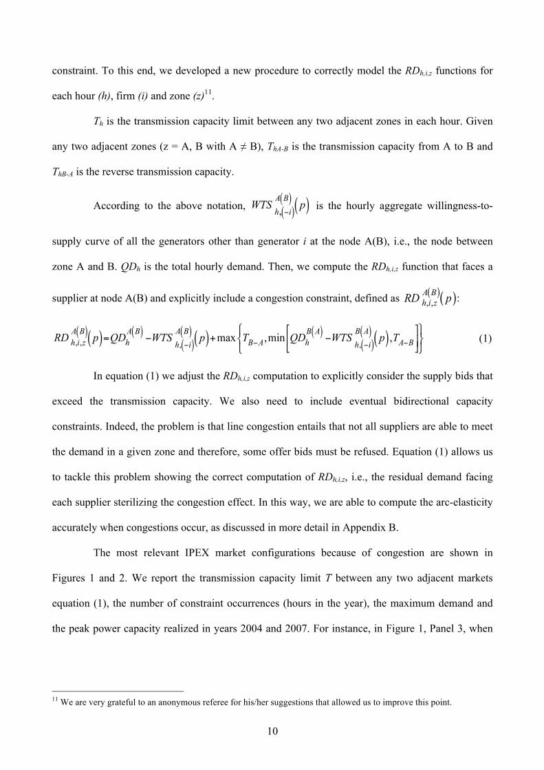
constraint. To this end, we developed a new procedure to correctly model the RDh,i,z functions for

each hour (h), firm (i) and zone (z)11.

Th is the transmission capacity limit between any two adjacent zones in each hour. Given

any two adjacent zones (z = A, B with A ≠ B), ThA-B is the transmission capacity from A to B and

ThB-A is the reverse transmission capacity.

According to the above notation, WTS h, −i( )A B( ) p( ) is the hourly aggregate willingness-to-

supply curve of all the generators other than generator i at the node A(B), i.e., the node between

zone A and B. QDh is the total hourly demand. Then, we compute the RDh,i,z function that faces a

supplier at node A(B) and explicitly include a congestion constraint, defined as ( )( ), ,A Bh i zRD p :

RD h,i,zA B( ) p( )=QDh

A B( ) −WTSh, −i( )A B( ) p( )+max TB−A,min QDh

B A( ) −WTSh, −i( )B A( ) p( ),TA−B

"

#$%

&'()*

+,-

(1)

In equation (1) we adjust the RDh,i,z computation to explicitly consider the supply bids that

exceed the transmission capacity. We also need to include eventual bidirectional capacity

constraints. Indeed, the problem is that line congestion entails that not all suppliers are able to meet

the demand in a given zone and therefore, some offer bids must be refused. Equation (1) allows us

to tackle this problem showing the correct computation of RDh,i,z, i.e., the residual demand facing

each supplier sterilizing the congestion effect. In this way, we are able to compute the arc-elasticity

accurately when congestions occur, as discussed in more detail in Appendix B.

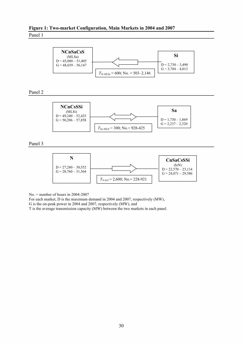
The most relevant IPEX market configurations because of congestion are shown in

Figures 1 and 2. We report the transmission capacity limit T between any two adjacent markets

equation (1), the number of constraint occurrences (hours in the year), the maximum demand and

the peak power capacity realized in years 2004 and 2007. For instance, in Figure 1, Panel 3, when

11 We are very grateful to an anonymous referee for his/her suggestions that allowed us to improve this point.

11

A=N and B=IeN, TA-B=2,600 and TB-A=0, on average because the transmission flows are

unidirectional.

Consider the most frequent congestion occurrence in the IPEX, which results in a two-

market configuration. This event can occur in three distinct ways (N, IeN; Si, MLSa; Sa, MLSi),

which account for 39% of the hours in the period (Figure 1). Although an surge of line congestion

between one of the islands, Si or Sa, and the rest of Italy is not completely surprising, the fact that

the N stands as a separate market from rest of Italy could be an indication of peculiar market

behavior because N accounts for one half of total Italian consumption, on average.

[Figure 1 here]

Note that these three segmentations occur when the flows exceed the transmission

capacity that lies between a minimum (average) value of T=300 MW in Panel 2 and a maximum

(average) value of T=2,600 MW in Panel 3. These constrained events represent at most 10% of total

hours. In this period, the number of hours of congestion between N and IeN and between Si and

MLSa increases, but the opposite occurs in the case of Sa and MLSi, while the ratio of peak

capacity to demand has increased in large zones. This follows from the inadequacy of transmission

line developments in the same period.

Focusing on the case of a three-market configuration, we consider the two most relevant

configurations, which account for 23.1% of the hours in the period (Figure 2): Si, Sa and ML; N, Si

and IeNSi. The first configuration appear to be less frequent as time passes, but the last one shows a

four-fold increase from 270 hours in 2004 to 1,162 hours in 2007. Moreover, demand in both Sa

and Si is generally higher when there is a two-market rather than a three-market configuration, but

the reverse is observed for N.

[Figure 2 here]

12

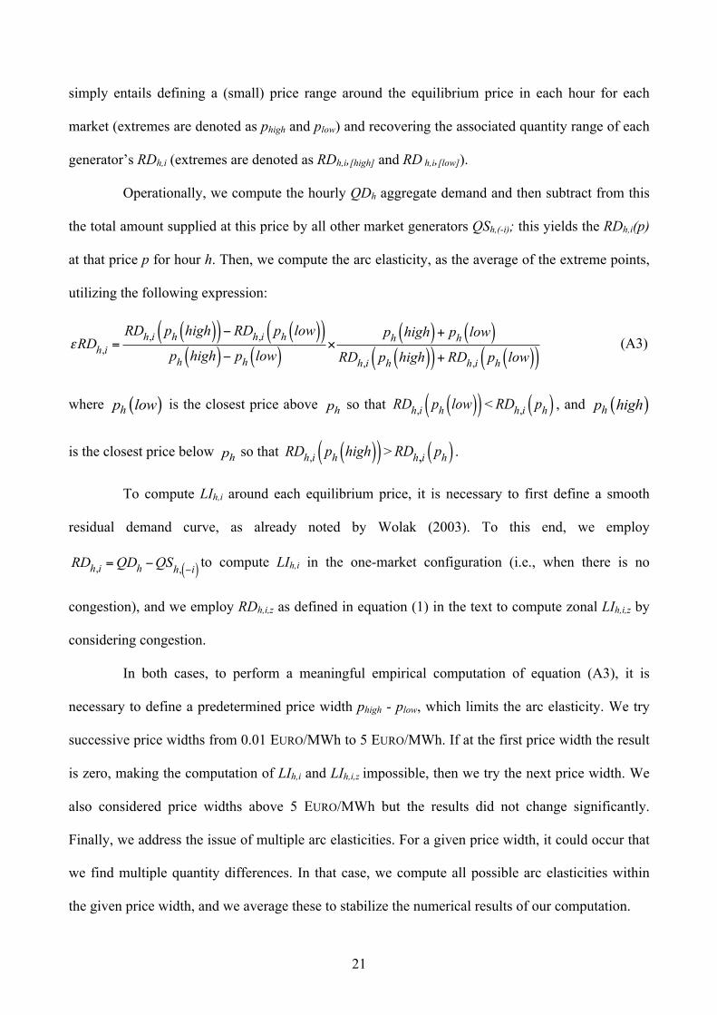
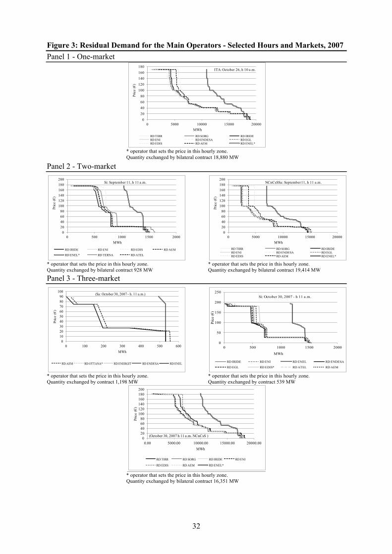
The computation of εRDh,i,z simply entails defining a (small) price range around the

equilibrium price in each hourly market zone (extremes are denoted as phigh and plow) and employing

the associated quantity range of each generator RDh,i,z (extremes are denoted as RDh,i,z[high] and

RDh,i,z[low]) according to equation (A3) of Appendix A.

The RDh,i,z computations for the main market operators for various market configurations

are shown in Figure 3. In detail, we report data for one-market (ITA), two-market (Si, MLSa) and

three-market configurations (Si, Sa, ML). Note that the RDh,i,z of ENEL, the former monopolist,

always lies to the furthest right and tends to be steeper than the others.

[Figure 3 here]

IV. EMPIRICAL ANALYSIS

We present our analysis of market power based on a computation of the unbiased LIh,i,z,

according to equation (A2) by considering the congestion issue by appropriately defining the RDh,i,z

as shown in equation (1).

We have computed LIh,i,z for a group of generators identified as marginal operators

according to the GME definition. ENEL is the most important marginal operator in the IPEX and

sets the price in 80% of the hours in all the market zones, on average (Appendix C). In addition to

ENEL, there are also marginal operators in some market zones. Endesa sets the price in Sa for more

than 50% of the hours; Edison sets the price in Si for more than 20% of the hours and in N for

approximately 9% of the hours. AEM also sets the price in N for approximately 9% of the hours.

Finally, ATEL set the price in Si for approximately 4% of the hours during the last two years.

We present the results for the generator and the main market configurations in Tables 6 and

7. The analysis of the IPEX shows that ENEL has the greatest market power in each market. In

13

particular, when there is no congestion (approximately 18% of the hours), ENEL’s LIh is 33%, on

average (Table 6). Moreover, the ENEL index decreased steadily in this period from 38% in 2004 to

28% in 2007.

[Table 6 here]

We claim that this result depends on (i) the increased number of operators, (ii) the increase

of ENEL’s foreign activities, especially in Eastern Europe, (iii) ENEL’s market share reduction, and

(iv) the increased generating capacity of ENEL’s competitors. Focusing on ENEL’s main

competitors, we note that their LIh is low and stable over the given time period.

When there is congestion, the picture changes somewhat (Table 7). We have summarized

the average unbiased LIh,i,z for the most important markets during line congestion, which are

presented in Figures 1 and 2 above. To simplify the presentation, we report the LIh,i,z values for the

eight most important markets. They are three PNZ (N, Si and Sa in Panel 1) and five interconnected

zones (Panel 2). Note that the reported values for N, Si and Sa are the averages12 of the unbiased

LIh,i,z that results from various segmentations. For instance, the value for N is the average of LIh,i,z

when N is a separate market from IeN (Figure 1, Panel 3) and a separate market from IeNSi and Si

(Figure 2, Panel 2). Because these differences are not significant for N, Si and Sa, we report only

the average values (Table 7, Panel 1).

We underline the prominent result for ENEL. In N, ENEL has a lower LIi,z than in ITA on

average. This is equal to 25%. However, in the same zone, AEM has a LIi,z of approximately 5%,

12 The yearly LIh,i,z computations for Table 7 demonstrate that the parameters are stable over time. In particular, in the

most frequent three-market configuration (ML, Si and Sa), ENEL’s LIh,i,z slightly decreases over time, but Edison in Si

and Endesa in Sa present slightly increasing LIh,i,z values. However, LIh,i,z differences in time are rejected by the mean

test for each generator.

14

and Endesa has a LIi,z of approximately 2.8%. ENEL’s LIi,z is even lower in other zones: 13% in the

zone of Central Italy (IeNSi), 11.7% in Si and 5% in Sa.

[Table 7 here]

There is evidence of market power exercised by other generators in the two-market

configuration. In the N-IeN segmentation (Figure 1, Panel 3), ENEL has a LIi,z of 25% in N and

26.1% in IeN (see the first row of Table 7, Panel 1 and 2, respectively), and AEM has values of

5.1% and 5.7%, respectively. Thus, when there is congestion between N and IeN, a duopoly

competition emerges between ENEL and AEM.

In the Si-MLSa segmentation (Figure 1, Panel 1), ENEL has a LIi,z of 11.7% in Si and 19.7%

in MLSa (see the second row of Table 7, Panel 1 and 2, respectively), and Edison has values of

5.8% and 6.7%, respectively. Thus, when there is congestion between Si and MLSa, a duopoly

competition emerges between ENEL and Edison. Similarly, in the Sa-MLSi segmentation (Figure 1,

Panel 2), ENEL has a LIi,z of only 4.9% in Sa and 22.3% in MLSi (see the third row of Table 7,

Panel 1 and 2, respectively), and Endesa has values of 10.5% and 9.7%, respectively. In this case,

there is a duopoly competition between ENEL and Endesa. This is the only situation in which

ENEL’s index is lower than that of one of its competitor’s in a given zone. This finding may help

the external observer rationalize the acquisition of Endesa by ENEL that took place at the end of

2008. With this acquisition, ENEL has strengthened its role as a global player in important

international markets such as Spain and Latin America but has also strengthened its position in the

Sardegna market. In fact, simultaneously with the acquisition of Endesa, ENEL sold one plant

owned by Endesa in Sardegna to AEM, which is certainly a smaller competitor than Endesa.

However, the most striking evidence of market power is found in the three-market

configuration. Note that ENEL’s LIi,z is 40% in ML (see the fourth row of Table 7, Panel 2), which

is the largest zone in the three-market configuration (Figure 2, Panel 1) where the other two markets

15

are Si and Sa. In Si, ENEL’s most important competitor, Edison, has a LIi,z of 5.8%. In Sa, ENEL’s

other significant competitor, Endesa, has a LIi,z, of 10.5%. These latter values are among the highest

values that Edison and Endesa have achieved in the various IPEX configurations.

Overall, this is a clear indication that the three-market configuration of ML, Si and Sa is the

least competitive configuration in the IPEX. In other words, when there is congestion among ML

and the islands, three generators are able to exercise their market power contemporaneously with

each having a relative maximum strength in a given zone: ENEL in ML, Edison in Si and Endesa in

Sa.

In the other three-market configuration, when N and Si are separated from IeNSi (see the

last row of Table 7, Panel 2), the LIi,z values range from 13.3% for ENEL to 8% for Endesa. Note

that Endesa retains significant market power when Sa is connected with the MLSi, which hints that

Endesa can exert relevant market power aggressiveness in that island irrespective of the market

configuration.

In summary, the results shown in Table 7 highlight that ENEL dominates the market in the

majority of the market segmentations, and Endesa has a higher LIi,z than that of ENEL in only Sa.

Other operators also emerge in specific markets, such as AEM in N and Edison in Si.

V. CONCLUSION

In this paper, we addressed the issue of analyzing market power in the IPEX from 2004 to

2007 utilizing hourly data provided by the GME. We employ market bid data by explicitly

considering congestions in the LI computations for the primary operators. The contribution of our

paper is to demonstrate and empirically measure that there are important differences in the

generators’ exercise of market power in the various zones of the IPEX.

ENEL, the former monopolist, shows a sizable market power when the Italian market is not

segmented and a mark-up of price over marginal cost of approximately 32%, but this decreases over

the period considered. This reveals that when maximum simultaneous competition is possible, i.e.,

16

when transmission is not congested, competition forces have worked in the sense that other

operators have become more aggressive over time. The outcome is that the one-market

configuration has become more competitive and that the oligopolistic mark-up of the former

monopolist decreased by 10 percentage points (from 38% to 28%) in four years. Other operators

exhibit a small market power that slightly increased over time.

Considering market segmentation, new results emerge from our analysis. There are certain

IPEX configurations, e.g., ML, Si and Sa, where all three major generators -ENEL, Edison and

Endesa retain appreciable market power (with zonal LI of 40%, 11% and 6%, respectively). Endesa

and Edison emerge as important players in the two islands, but ENEL is also able to exert a higher

market power in ML. Notice that this IPEX configuration frequency shown a dramatic four-fold

increase in the period analyzed. Overall, these results reveal the inadequacy of the transmission

network development in this period. Our analysis reveals that competition works when the market is

unique but that the hours in which segmentation favors market power have increased due to

structural line congestion. There has been a sort of “live-and-let live” combined behavior of the

generators and transmission network, which has certainly delayed the competitive development of

the Italian electric market at the initial stage of its liberalization.

In conclusion, there are interesting policy implications of our analysis of the initial period 2004-

2007 of liberalization of the Italian market. We deem that the empirical measure of the exercise of

zonal market power is a useful instrument for the regulator, in order to enact more efficient policy

measures. In other words, focusing the attention to specific zones allows the regulator to design an

optimal portfolio intervention. In fact, if market power occurs in cases without market splitting, the

regulator should surely enact pro-competitive measures. Alternatively, when market power is

associated with line congestion in specific zones, the regulator should consider also transmission

network development incentive measures, such as preferential rate-of-return targets for new lines.

These issues are particularly important for many areas in the world, which are now in an early stage

of liberalization, like the Italian situation in the period 2004-2007. Our research paves the way of

17

possible directions for future research. In the Italian market, as well as in many electricity markets,

there has recently been booming development of RES, which deserves careful analysis, as abundant

RES supply may result in lower equilibrium prices, thereby deceiving the analysis of market power

effects. Moreover, it would be interesting to explore the relationships between zonal market power

and fuel price trends to assess whether specific generation mix structurally influences market

power. We leave these issues for future research.

REFERENCES

Baker, Jonathan (1988). “Estimating the Residual Demand Curve Facing a Single Firm.”

International Journal of Industrial Organization, 6(3): 283-300.

Bigerna, Simona, and Paolo Polinori (2014). “Italian Households’ Willingness to Pay for Green

Electricity.” Renewable and Sustainable Energy Review, 34(June): 110-121.

Boffa, Federico, Viswanath Pingali, and Davide Vannoni (2010). “Increasing Market

Interconnection. An Analysis of the Italian Electricity Spot Market.” International Journal

of Industrial Organization, 28(3): 311-322.

Bollino, C. Andrea, and Paolo Polinori (2008). “Measuring Market Power in Wholesale Italian

Electricity Markets.” SSRN Working Papers. Document Available online at:

http://papers.ssrn.com/sol3/papers.cfm?abstract_id=1129202.

Borenstein, Severin, James B. Bushnell, and Frank A. Wolak (2002). “Measuring Market

Inefficiencies in California's Restructured Wholesale Electricity Market.” American

Economic Review, 92(5): 1376-1405.

Bosco, Bruno, Lucia Parisio, and Marco Pelagatti (2012). “Strategic Bidding in Vertically

Integrated Power Markets with an Application to the Italian Electricity Auctions.” Energy

Economics, 34(6): 2046-2057.

18

Cho, In-Koo, and Hyunsook Kim (2007) “Market Power and Network Constraint in a Deregulated

Electricity Market.” The Energy Journal, 28(2): 1-34.

Karthikeyana, S. Prabhakar, I. Jacob Raglendb, and Dwarkadas P. Kothari (2013). “A Review on

Market Power in Deregulated Electricity Market.” International Journal of Electrical Power

& Energy Systems, 48(Jun): 139–147.

Gianfreda, Angelica, and Luigi Grossi (2012). “Forecasting Italian Electricity Zonal Prices with

Exogenous Variables.” Energy Economics, 34(Nov): 2228–2239.

GME (2004-2007) “Annual Report.” Documents Available online at:

http://www.mercatoelettrico.org/en/GME/Biblioteca/RapportiAnnuali.aspx

Lee, Yen-Yu, Jin Hur, Ross Baldick, and Salvador Pineda (2011). “New Indices of Market Power in

Transmission-Constrained Electricity Markets.” IEEE TRANSACTIONS ON POWER

SYSTEMS, 26(2). Document available on line at:

http://ieeexplore.ieee.org/stamp/stamp.jsp?tp=&arnumber=5557794

Lerner, Abba (1934). “The Concept of Monopoly and the Measurement of Market Power.” Review

of Economics and Statistics, 1(3): 157-75.

McRae, Shaun D., and Frank A. Wolak (2009). “How Do Firms Exercise Unilateral Market Power?

Evidence from a Bid-Based Wholesale Electricity Market.” Series/Report no.: EUI RSCAS;

2009/36; Loyola De Palacio Programme on Energy Policy. ISSN: 1028-3625. Document

available on line at: http://hdl.handle.net/1814/12098

Mirza, Faisal M., and Olvar, Bergland (2012). “Pass-through of Wholesale Price to the End User

Retail Price in the Norwegian Electricity Market.” Energy Economics, 34(6): 2003 – 2012.

Nappu, Muhammad B., Ramesh C. Bansal, and Tapan K. Saha (2013). “Market Power Implication

on Congested Power System: A Case Study of Financial Withheld Strategy” International

Journal of Electrical Power & Energy Systems, 47(May), 408 – 415.

Newbery, David (2005). “Electricity Liberalisation in Britain: the Quest for a Satisfactory

Wholesale Market Design.” The Energy Journal, (Special issue): 43-70.

19

Petrella, Andrea, and Alessandro Sapio (2012). “Assessing the Impact of Forward Trading, Retail

Liberalization, and White Certificates on the Italian Wholesale Electricity Prices.” Energy

Policy 40(Jan): 307–317.

Perekhodtsev, Dimitri, and Rossella Baselice (2010). “Empirical Assessment of Strategic Behavior

in the Italian Power Exchange.” Electrical Energy System, 21(6): 1842-1855.

Shukla, Umesh K., and Ashok, Thampy (2011). “Analysis of Competition and Market Power in the

Wholesale Electricity Market in India.” Energy Policy, 39(5): 2699 – 2710.

Sweeting, Andrew (2007). “Market Power in the England and Wales Wholesale Electricity Market

1995-2000.” The Economic Journal, 117(520): 654-685.

Wolak, Frank A. (2000). “An Empirical Analysis of the Impact of Hedge Contracts on Bidding

Behavior in a Competitive Electricity Market.” International Economic Journal, 14(2): 1-

40.

Wolak, Frank A. (2003). “Measuring Unilateral Market Power in Wholesale Electricity Markets:

the California Market, 1988-2000.” American Economic Review, 93(2): 425-430.

Wolak, Frank A. (2009). “Report on Market Performance and Market Monitoring in the Colombian

Electricity Supply Industry.” Document available online at:

http://www.stanford.edu/group/fwolak/cgi/bin/sites/default/files/files/sspd_report_wolak_jul

y_30.pdf

Wolak, Frank A. (2012). Measuring the Competitiveness Benefits of a Transmission Investment

Policy: The Case of the Alberta Electricity Market. Document available online at:

http://web.stanford.edu/group/fwolak/cgibin/sites/default/files/files/alberta_transmission_be

nefits.pdf

20

APPENDIX A: THE THEORETICAL MODEL

The standard theoretical framework to measure unilateral firm-level market power without

congestions is characterized the assumption that a firm chooses the best pricing strategy by

considering the residual demand (RD), i.e., considering the bids submitted by all other competitors

for each firm i. We can write the firm profit (Π) function as follows:

Πh,i = RDh,i ( ph ) ⋅ ( ph −MCh,i )− ( ph − pch,i ) ⋅QCh,i − Fi (A1)

where ph is the hourly spot price, pchi is the price of contract, Fi is the fixed cost, MCh,i is the

marginal cost, RDh,i =QDh −QSh, −i( ) , where QDh is the total demand, QSh,(-i) is the supply of all the

other competitors and QCh,i is the quantity exchanged by contracts. In other words, the first term is

the variable profit obtained in the spot market; the second term is the profit generated from

contracts sales and purchasing activities on the forward market. Given that pch,i is not required for

maximization, we have subtracted QCh,i from RDh,i for each hour and operator (Bosco et al. 2012).

In this way, we have computed the correct arc elasticity using the un-contracted quantity, which is

the quantity net of contract for differences. We have recorded the contracted electricity exchange

supply for each operator, and then, we have appropriately assigned these quantities according to the

market’s segmentation. In this way, we can compute the residual un-contracted demand. Obviously,

profit maximization with respect to p yields (Lerner 1934):

ph −MCh,iph

= −1

εRDh,i= LIh,i (A2)

where εRDh,i is the hourly elasticity of RDh,i for each firm i (Wolak 2003). All these computations

hold for each state of demand; typically, it is assumed to hold for each hour of an hourly market.

The attractiveness of equation (A2) is that it is quite easy to compute the elasticity of RDh,i for each

firm given all the other competitors’ bids in a market such as the Italian electricity market described

above. Equation (A2) allows for the interpretation of the computed value of LIh,i as a measure of

unilateral market power exercised by firm i in each state. Operationally, the computation of εRDh,i

21

simply entails defining a (small) price range around the equilibrium price in each hour for each

market (extremes are denoted as phigh and plow) and recovering the associated quantity range of each

generator’s RDh,i (extremes are denoted as RDh,i,[high] and RD h,i,[low]).

Operationally, we compute the hourly QDh aggregate demand and then subtract from this

the total amount supplied at this price by all other market generators QSh,(-i); this yields the RDh,i(p)

at that price p for hour h. Then, we compute the arc elasticity, as the average of the extreme points,

utilizing the following expression:

εRDh,i =RDh,i ph high( )( )− RDh,i ph low( )( )

ph high( )− ph low( )×

ph high( )+ ph low( )RDh,i ph high( )( )+ RDh,i ph low( )( )

(A3)

where ( )hp low is the closest price above hp so that RDh,i ph low( )( ) < RDh,i ph( ) , and ( )hp high

is the closest price below hp so that RDh,i ph high( )( ) > RDh,i ph( ) .

To compute LIh,i around each equilibrium price, it is necessary to first define a smooth

residual demand curve, as already noted by Wolak (2003). To this end, we employ

RDh,i =QDh −QSh, −i( ) to compute LIh,i in the one-market configuration (i.e., when there is no

congestion), and we employ RDh,i,z as defined in equation (1) in the text to compute zonal LIh,i,z by

considering congestion.

In both cases, to perform a meaningful empirical computation of equation (A3), it is

necessary to define a predetermined price width phigh - plow, which limits the arc elasticity. We try

successive price widths from 0.01 EURO/MWh to 5 EURO/MWh. If at the first price width the result

is zero, making the computation of LIh,i and LIh,i,z impossible, then we try the next price width. We

also considered price widths above 5 EURO/MWh but the results did not change significantly.

Finally, we address the issue of multiple arc elasticities. For a given price width, it could occur that

we find multiple quantity differences. In that case, we compute all possible arc elasticities within

the given price width, and we average these to stabilize the numerical results of our computation.

22

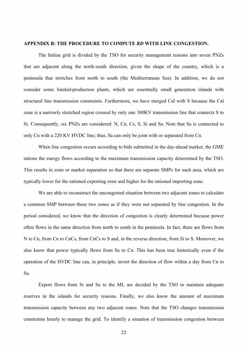
APPENDIX B: THE PROCEDURE TO COMPUTE RD WITH LINE CONGESTION.

The Italian grid is divided by the TSO for security management reasons into seven PNZs

that are adjacent along the north-south direction, given the shape of the country, which is a

peninsula that stretches from north to south (the Mediterranean Sea). In addition, we do not

consider some limited-production plants, which are essentially small generation islands with

structural line transmission constraints. Furthermore, we have merged Cal with S because the Cal

zone is a narrowly stretched region crossed by only one 380KV transmission line that connects S to

Si. Consequently, six PNZs are considered: N, Cn, Cs, S, Si and Sa. Note that Sa is connected to

only Cn with a 220 KV HVDC line; thus, Sa can only be joint with or separated from Cn.

When line congestion occurs according to bids submitted in the day-ahead market, the GME

rations the energy flows according to the maximum transmission capacity determined by the TSO.

This results in zone or market separation so that there are separate SMPs for each area, which are

typically lower for the rationed exporting zone and higher for the rationed importing zone.

We are able to reconstruct the uncongested situation between two adjacent zones to calculate

a common SMP between these two zones as if they were not separated by line congestion. In the

period considered, we know that the direction of congestion is clearly determined because power

often flows in the same direction from north to south in the peninsula. In fact, there are flows from

N to Cn, from Cn to CnCs, from CnCs to S and, in the reverse direction, from Si to S. Moreover, we

also know that power typically flows from Sa to Cn. This has been true historically even if the

operation of the HVDC line can, in principle, invert the direction of flow within a day from Cn to

Sa.

Export flows from Si and Sa to the ML are decided by the TSO to maintain adequate

reserves in the islands for security reasons. Finally, we also know the amount of maximum

transmission capacity between any two adjacent zones. Note that the TSO changes transmission

constraints hourly to manage the grid. To identify a situation of transmission congestion between

23

two adjacent zones, we preliminarily check that there are rejected bids at a price below the SMP in

the lower SMP zone (exporting zone) of the higher SMP zone (importing zone). This is the

indication that these bids could have been accepted by the GME to serve the load in the importing

zone if there were not line transmission congestion. We employ as a benchmark the TSO technical

measure of line congestion, which indicates the maximum capacity for security reasons because it

provides an upper limit to the effective hourly congestion. In other words, we are sure that in this

way, in every hour and in every zone, we could consider all bids rejected because of congestion.

Thus, we do not need to know the exact amount of capacity congestion every hour because it is

sufficient to know only that congestion arises between two adjacent zones, which yields a SMP

differential. We implement the computing algorithm of equation (1) in the text as follows.

First, we check for different values for the SMP each hour. There are three cases. (i)

Congestions do not occur and consequently, there is a one-market configuration, and Italy is a

unique zone. (ii) There is a two-market configuration with five possible aggregation schemes (as

reported in Table 3). (iii) There is a three-market configuration with ten possible aggregation

schemes (reported in Table 3), given the shape of the Italian grid.

These three cases constitute approximately 89% of the total. Therefore, we have not

computed εDR, h,i in cases of a four- or more-market configuration.

Second, we consider any two adjacent zones with different SMPs (adjacent markets), and we

identify all the rejected bids made by units located in the lower SMP zone (exporting zone) with a

bid price lower than the SMP of the other zone (importing zone). These latter bids are evidently

bids that were rationed and therefore, could not be put in the merit order because of transmission

capacity constraints.

Third, we consider all the accepted bids made by units located in the higher SMP zone

(importing zone) with a bid price higher than the SMP of the other zone. These latter bids are

evidently put in the merit order due to transmission constraints because they bid a price higher than

the SMP of the other zone.

24

Fourth, we reinsert bids identified above in the merit order of the new simulated zone that

results from merging the two adjacent zones. In this way, we construct a simulated common SMP

for the two adjacent zones. This simulated SMP must lie between the two adjacent zonal SMPs

because it is constructed by accepting the lower cost bids from the exporting zone and rejecting the

higher cost bids from the importing zone. We merge these adjacent zones to identify which would

be the simulated common SMP, as if there were no transmission constraint. Finally, we compute

RD and the related elasticity around the simulated SMP.

Note that in the last three phases of the algorithm, we have therefore controlled for the

effects of the network constraints on the merit order. In detail, we have generated a new merit order

that reproduces a simulated market outcome without congestion. We have done so including both

accepted bids above the SMP and rejected bids below the SMP.

Some caveats are in order. We have employed the technical TSO transmission capacity

during the entire year. This is not a severe problem, although we neglect the summer-winter

capacity variation due to temperature differences. Moreover, we are able to implement this

procedure by taking into consideration only two zones at a time. This means that this procedure is

certainly correct for the two-market configuration, but it can be considered a good approximation if

there are three or more hourly markets because we take into consideration bids only between two

adjacent zones.

To clarify this with a practical example, if the three markets are N, Si and IeNSi, we can

implement our procedure by considering N and the rest of the market transmission constraints and

Si and the rest of the market transmission constraints sequentially. This means that we would not be

able to identify a bid located in N that can be accepted in the merit order in Si (which is a non-

adjacent zone to N). Given the shape of Italy, the geographical distance among non-adjacent zones

is quite significant. Consequently, this problem is heuristically existent but of negligible

quantitative impact on the empirical results.

25

In addition, we make use of the difference between the actual SMP in any two adjacent

separated zones and the virtual common SMP to disentangle the effect of congestion from the effect

of the exercise of the unilateral market power of the generators. Thus, our measure of congestion

should not be confused with the congestion rent computed by the TSO.

APPENDIX C: STATISTICAL INFORMATION

To compute LIh,i and LIh,i,z we had to address a large data set of raw data made available by

the GME. We have preliminarily filtered the day-ahead market data, which typically consists of

approximately 60,000 records per day; this means that our full data set contains approximately

82,260,000 records for the period of 2004-2007.

We have run a sequence of VBA programs on elementary Access and Excel data sets. We

have used Access to manage the entire dataset as a relational dataset. This allows better control for

mistakes in recoded and missing values treatment. The first VBA program builds a cumulative

demand and price bids for each generator according to merit order in various markets (this step

requires approximately 160 man-hours of work for each year in the period analyzed).

The second VBA program identifies bids for each elementary zone and PNZ for all possible

IPEX configurations. Each elementary zone is identified as the union of all bids with a unique

awarded SMP. In this step, the program also checks for additional “physical markets” in which a

plant located in the virtual zone or in a limited pole sets the price for a PNZ and includes these

additional “physical markets” in the database (this step requires approximately 120 man-hours of

work for each year in the period analyzed).

The third VBA program splits the full dataset into sub-datasets according to the various zone

segmentations. In practice, all the bids of each hourly market are marked as belonging to a unique

SMP. The program also performs checks for the correctness of the data obtained (this step requires

approximately 24 man-hours of work for each year in the period analyzed).

26

The fourth VBA program computes the RDh,i and RDh,i,z (RD) for each generator, the RD arc

elastic for various price ranges and the zonal LI for each generator. Specifically, the program checks

for the non-negativity of RD, the correctness of the segmented merit order, and the correctness of

the merit order of each computed elasticity according to the elementary geographical zones and

generator to with they belong (this step requires approximately 120 man-hours of work for each

zone-segmentation and each year in the period analyzed).

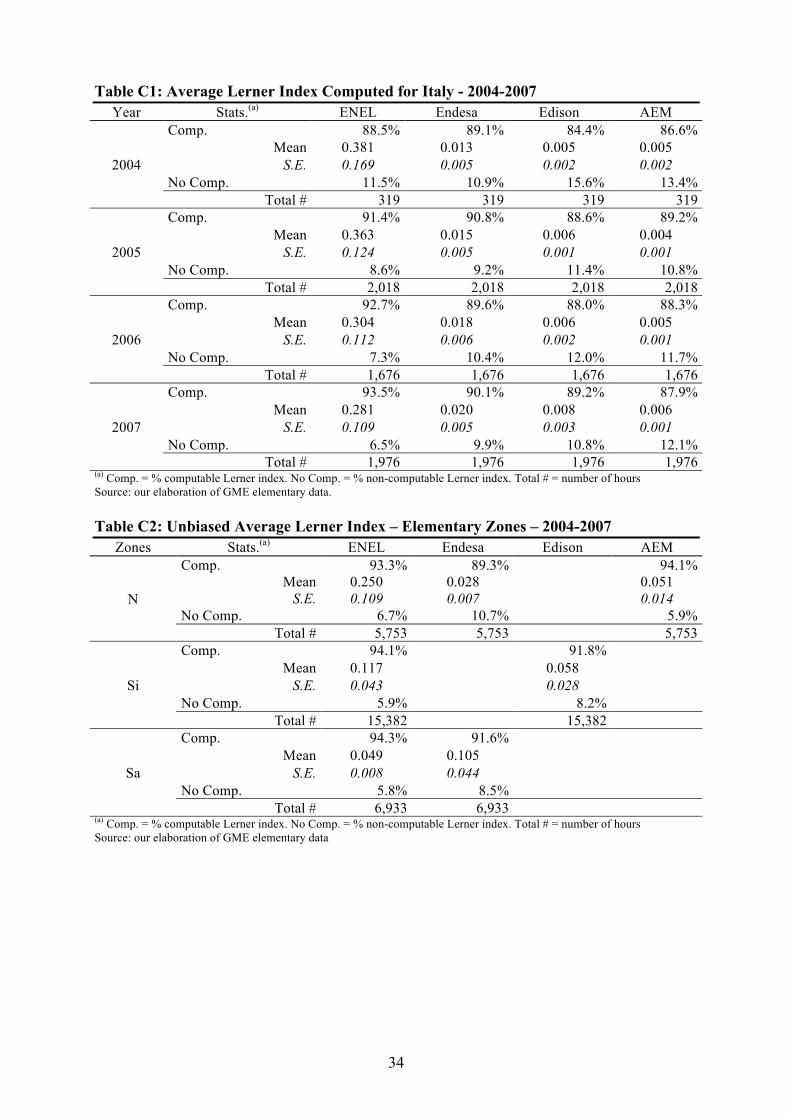
The average LI computations for the main generators are presented in Tables C1 – C3. In

each table, we present the average values, their standard errors and the percentage of non-

computable hours of the total hours (which is below 10-15% in all cases). We note that all the

computed average LI values are statistically significant at a 5% confidence level.

[Table C1 here]

[Table C2 here]

[Table C3 here]

ACKNOWLEDGMENTS

Preliminary versions of this paper were presented at the following conferences: the 25th

Annual North American Conference of the USAEE/IAEE, Denver, Colorado (USA), September 18-

21, 2005; the 29th IAEE International Conference, Potsdam (Germany), June 7-10, 2006; the 9th

IAEE European Energy Conference, Florence (Italy), June 10-12, 2007; the IDEI conference “The

Economics of Energy Markets,” Toulouse (France), June 20-21, 2008. We are indebted to all the

participants of these conferences. The authors are also thankful to Federico Boffa, Paolo Bruno

Bosco, Matteo Pelagatti, Marie Anne Plagnet, Lucia Visconti Parisio and three anonymous

reviewers for their helpful suggestions and remarks. Finally, we would like to thank Nicolino

“Nico” Gioffreda for research assistance. The usual disclaimer applies.

27

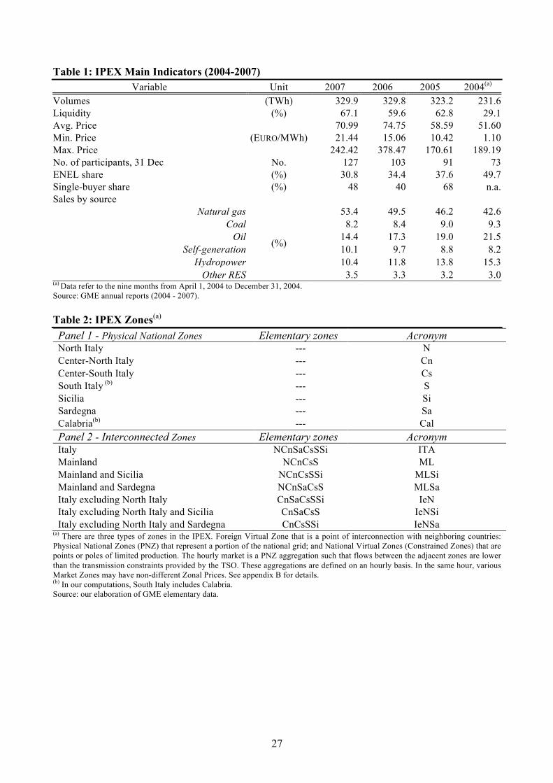
Table 1: IPEX Main Indicators (2004-2007) Variable Unit 2007 2006 2005 2004(a)

Volumes (TWh) 329.9 329.8 323.2 231.6 Liquidity (%) 67.1 59.6 62.8 29.1 Avg. Price

(EURO/MWh) 70.99 74.75 58.59 51.60

Min. Price 21.44 15.06 10.42 1.10 Max. Price 242.42 378.47 170.61 189.19 No. of participants, 31 Dec No. 127 103 91 73 ENEL share (%) 30.8 34.4 37.6 49.7 Single-buyer share (%) 48 40 68 n.a. Sales by source

Natural gas

(%)

53.4 49.5 46.2 42.6 Coal 8.2 8.4 9.0 9.3

Oil 14.4 17.3 19.0 21.5 Self-generation 10.1 9.7 8.8 8.2

Hydropower 10.4 11.8 13.8 15.3 Other RES 3.5 3.3 3.2 3.0

(a) Data refer to the nine months from April 1, 2004 to December 31, 2004. Source: GME annual reports (2004 - 2007). Table 2: IPEX Zones(a) Panel 1 - Physical National Zones Elementary zones Acronym North Italy --- N Center-North Italy --- Cn Center-South Italy --- Cs South Italy (b) --- S Sicilia --- Si Sardegna --- Sa Calabria(b) --- Cal Panel 2 - Interconnected Zones Elementary zones Acronym Italy NCnSaCsSSi ITA Mainland NCnCsS ML Mainland and Sicilia NCnCsSSi MLSi Mainland and Sardegna NCnSaCsS MLSa Italy excluding North Italy CnSaCsSSi IeN Italy excluding North Italy and Sicilia CnSaCsS IeNSi Italy excluding North Italy and Sardegna CnCsSSi IeNSa

(a) There are three types of zones in the IPEX. Foreign Virtual Zone that is a point of interconnection with neighboring countries: Physical National Zones (PNZ) that represent a portion of the national grid; and National Virtual Zones (Constrained Zones) that are points or poles of limited production. The hourly market is a PNZ aggregation such that flows between the adjacent zones are lower than the transmission constraints provided by the TSO. These aggregations are defined on an hourly basis. In the same hour, various Market Zones may have non-different Zonal Prices. See appendix B for details. (b) In our computations, South Italy includes Calabria. Source: our elaboration of GME elementary data.

28

Table 3: IPEX Markets According to Various Zone Configurations (2004-2007) (a, b, c)

Markets

Four-market Markets > 4

Nz ≥ 4 N

CnCsS Sa Si

NCn Sa

CsS Si

N CnSa CsS Si

N Cn Sa

CsSSi

N CnCs

Sa SSi

N CnSaCs

S Si

NCnCs Sa S Si

NCn Sa Cs SSi

Others(d)

No. of hours 2,098 884 146 100 22 20 6 1

110 3,351 % 6.381 2.689 0.444 0.304 0.067 0.061 0.018 0.003

0.335 10.19

Markets (e) Three-market

Nz = 3 NCnCsS Sa Si

N CnSaCsS

Si

N CnCsSSi

Sa

NCn Sa

CsSSi

NCnSa CsS Si

N CnSa CsSSi

NCnSaCs S Si

N CnSaCs

SSi

NCnCs Sa SSi

NCnSa Cs SSi

No. of hours 4,260 3,347 1,496 808 365 86 24 12 8 2 10,408 % 12.956 10.179 4.550 2.457 1.110 0.262 0.073 0.036 0.024 0.006 31.65

Markets (f) Two-market

Nz = 2 NCnSaCsS Si

NCnCsSSi Sa

N CnSaCsSSi

NCnSa CsSSi

NCnSaCs SSi

No. of hours 7,775 2,673 2,406 261 17

13,132 % 23.647 8.130 7.318 0.794 0.052

39.94

Markets One-market Nz = 1 ITA No. of hours 5,989

5,989 % 18.215

18.21

Total No. of hours from April 1st 2004 to December 31st 2007 (Total No. of market zones is 77,004) 32,880 (a) The various markets for each market configuration are on different lines in each Panel (4 lines for the four-market configuration and so on). (b) The most frequently markets are Si (57.5%), Sa (37.9%), N (29.2%), NCnSaCsS (23.7%) and NCnCsS (13.0%). (c) The average number of markets is 2.34. (d) We do not report the entire possible five- and six-market configuration in detail because they occur in a negligible share of the total hours. (e) The first two configurations occur in 23.1% of the hours. (f) The first three configurations occur in 39.1% of the hours. Source: our elaboration of GME elementary data

Table 4: IPEX Equilibrium Prices by Hourly Market

Configuration 2004 2005 2006 2007 Total Var. Price Price Var. Price Var. Price Var.

One-market (Avg.) 43.48 59.46 36.7% 73.91 24.3% 51.13 -30.8% 14.0% Two-market (Avg.) 47.56 57.91 21.8% 71.35 23.2% 70.52 -1.2% 21.8% Three-market (Avg.) 51.72 58.66 13.4% 77.89 32.8% 83.29 6.9% 42.0% Four-market (Avg.) 57.32 59.34 3.5% 84.38 42.2% 88.66 5.1% 49.4% Nz > 4 (Avg.) 56.82 67.29 18.4% 112.41 67.1% 104.46 -7.1% 55.2% Source: our elaboration of GME elementary data. (EURO/MWh) Table 5: IPEX Equilibrium Prices in the Main Markets(a)

Configuration Mean St. Dev. Min Max One-market (No. of hours 5,989)

ITA ITA 59.90 31.25 20.45 199.07 Two-market (No. of hours 13,132)

NCnCsSSa-Si NCnCsSSa (MLSa) 62.47 30.59 20.20 239.57 7,775 Si 68.85 35.79 0.00 290.22

NCnCsSSi-Sa NCnCsSSi (MLSi) 54.08 31.27 0.00 199.11 2,673 Sa 66.90 39.86 21.40 229.10

N-CnSaCsSSi N 74.65 34.36 0.00 198.20 2,406 CnSaCsSSi (IeN) 81.92 35.12 21.70 198.50

Three-market (No. of hours 10,408) NCnCsS-Sa-Si NCnCsS (ML) 55.39 34.39 0.00 400.00

4,260 Sa 66.13 41.66 21.50 250.32

SI 62.20 44.10 0.00 500.00

N-CnSaCsS-Si N 75.88 32.20 21.00 198.50 3,347 CnSaCsS (IeNSi) 83.91 35.37 21.40 199.27

Si 93.22 40.86 21.50 250.00 (a) The number of hours considered is 26,450, which is 80.4% of the total hours. (EURO/MWh) Source: our elaboration of GME elementary data.

30

Figure 1: Two-market Configuration, Main Markets in 2004 and 2007

Panel 1

Panel 2

Panel 3

No. = number of hours in 2004-2007 For each market, D is the maximum demand in 2004 and 2007, respectively (MW), G is the on-peak power in 2004 and 2007, respectively (MW), and T is the average transmission capacity (MW) between the two markets in each panel.

NCnSaCsS (MLSa)

D = 45,080 – 51,405 G = 48,659 – 56,147

Si D = 2,730 – 3,490 G = 3,784 – 4,013

TSi-MLSa = 600; No. = 503–2,146

NCnCsSSi (MLSi)

D = 49,240 – 52,425 G = 50,206 – 57,858

Sa D = 1,730 – 1,869 G = 2,237 – 2,320

TSa-MLSi = 300; No.= 928-425

N

D = 27,280 – 30,552 G = 28,760 – 31,564

CnSaCsSSi (IeN)

D = 22,570 – 23,114 G = 24,071 – 29,586

TN-IeN = 2,600; No.= 228-921

31

Figure 2: Three-market Configuration, Main Markets in 2004 and 2007

Panel 1

Panel 2

No.=number of hours in 2004-2007 For each market, D is the maximum demand in 2004 and 2007, respectively (MW), G is the on-peak power in 2004 and 2007, respectively (MW), and T is the average transmission capacity (MW) between any two adjacent markets.

NCnCsS (ML)

D = 45,270 – 49,749 G = 46,422 – 53,845

Si D = 2,940 – 3,441 G = 3,784 – 4,013

TSi-ML = 600 TSa-ML = 300 No. = 1874 – 866

Sa D = 1,690 – 1,837 G = 2,237 – 2,320

CnSaCsS (IeNSi)

D = 30,122 – 20,746 G = 19,900 – 24,600

Si D = 2,830 – 3,312 G = 3,784 – 4,013

TSi-IeNSI = 600 TN-IeNSi = 2,600 No. = 270 – 1,162

N D = 26,450 – 30,122 G = 28,760 – 31,564

32

Figure 3: Residual Demand for the Main Operators - Selected Hours and Markets, 2007

Panel 1 - One-market

* operator that sets the price in this hourly zone. Quantity exchanged by bilateral contract 18,880 MW

Panel 2 - Two-market

* operator that sets the price in this hourly zone. Quantity exchanged by bilateral contract 928 MW

* operator that sets the price in this hourly zone. Quantity exchanged by bilateral contract 19,414 MW

Panel 3 - Three-market

* operator that sets the price in this hourly zone. Quantity exchanged by contract 1,198 MW

* operator that sets the price in this hourly zone. Quantity exchanged by contract 539 MW

* operator that sets the price in this hourly zone. Quantity exchanged by bilateral contract 16,351 MW

020406080

100120140160180

0 5000 10000 15000 20000

Pric

e (€

)MWh

ITA: October 26, h 10 a.m.

RD TIRR RD SORG RD IRIDERD ENI RD ENDESA RD EGLRD EDIS RD AEM RD ENEL*

020406080

100120140160180200

0 500 1000 1500 2000

Pric

e (€

)

MWh

Si: September 11, h 11 a.m.

RD IRIDE RD ENI RD EDIS RD AEM

RD ENEL* RD TERNA RD ATEL

020406080

100120140160180200

0 5000 10000 15000 20000

Pric

e (€

)

MWh

NCnCsSSa: September 11, h 11 a.m.

RD TIRR RD SORG RD IRIDERD ENI RD ENDESA RD EGLRD EDIS RD AEM RD ENEL*

0102030405060708090

100

0 100 200 300 400 500 600

Pric

e (€

)

MWh

(Sa: October 30, 2007 - h. 11 a.m.)

RD AEM RD OTTANA* RD ENERGIT RD ENDESA RD ENEL

0

50

100

150

200

250

0 500 1000 1500 2000

Price

(€)

MWh

Si: October 30, 2007 - h 11 a.m.

RD IRIDE RD ENI RD ENEL RD ENDESA

RD EGL RD EDIS* RD ATEL RD AEM

020406080

100120140160180200

0.00 5000.00 10000.00 15000.00 20000.00

Pric

e (€

)

MWh

(October 30, 2007 h 11 a.m. NCnCsS )

RD TIRR RD SORG RD IRIDE RD ENI

RD EDIS RD AEM RD ENEL*

Table 6: One-market Configuration (ITA), Average Annual Lerner Index

Generator 2004 2005 2006 2007 2004-2007 (Avg.)

ENEL 0.381 0.363 0.304 0.281 0.3332 Endesa 0.013 0.015 0.018 0.021 0.0164 Edison 0.005 0.006 0.006 0.008 0.0062 AEM 0.005 0.004 0.005 0.006 0.0049 Source: our elaboration of GME elementary data Table 7: Average Unbiased Lerner Index by Markets - 2004-2007

ENEL Endesa Edison AEM Panel 1- Physical National Zones(a)

N 0.250 0.028

0.051 Si 0.117

0.058

Sa 0.049 0.105 Panel 2 – Interconnected Zones

CnSaCsSSi (IeN) 0.261

0.057 NCnSaCsS (MLSa) 0.195

0.067

NCnCsSSi (MLSi) 0.223 0.097 NCnCsS (ML) 0.402 0.021

0.022 CnSaCsS (IeNSi) 0.133 0.081

(a) We report the average Lerner index in each market; for instance, the value for ENEL in N is the average of N belonging to a two- and three-market configuration. Source: our elaboration of GME elementary data.

34

Table C1: Average Lerner Index Computed for Italy - 2004-2007 Year Stats.(a) ENEL Endesa Edison AEM

2004

Comp. 88.5% 89.1% 84.4% 86.6% Mean 0.381 0.013 0.005 0.005

S.E. 0.169 0.005 0.002 0.002 No Comp. 11.5% 10.9% 15.6% 13.4%

Total # 319 319 319 319

2005

Comp. 91.4% 90.8% 88.6% 89.2% Mean 0.363 0.015 0.006 0.004

S.E. 0.124 0.005 0.001 0.001 No Comp. 8.6% 9.2% 11.4% 10.8%

Total # 2,018 2,018 2,018 2,018

2006

Comp. 92.7% 89.6% 88.0% 88.3% Mean 0.304 0.018 0.006 0.005

S.E. 0.112 0.006 0.002 0.001 No Comp. 7.3% 10.4% 12.0% 11.7%

Total # 1,676 1,676 1,676 1,676

2007

Comp. 93.5% 90.1% 89.2% 87.9% Mean 0.281 0.020 0.008 0.006

S.E. 0.109 0.005 0.003 0.001 No Comp. 6.5% 9.9% 10.8% 12.1%

Total # 1,976 1,976 1,976 1,976 (a) Comp. = % computable Lerner index. No Comp. = % non-computable Lerner index. Total # = number of hours Source: our elaboration of GME elementary data. Table C2: Unbiased Average Lerner Index – Elementary Zones – 2004-2007

Zones Stats.(a) ENEL Endesa Edison AEM

N

Comp. 93.3% 89.3%

94.1% Mean 0.250 0.028

0.051

S.E. 0.109 0.007

0.014 No Comp. 6.7% 10.7%

5.9%

Total # 5,753 5,753 5,753

Si

Comp. 94.1%

91.8% Mean 0.117

0.058

S.E. 0.043

0.028 No Comp. 5.9%

8.2%

Total # 15,382 15,382

Sa

Comp. 94.3% 91.6% Mean 0.049 0.105 S.E. 0.008 0.044 No Comp. 5.8% 8.5% Total # 6,933 6,933

(a) Comp. = % computable Lerner index. No Comp. = % non-computable Lerner index. Total # = number of hours Source: our elaboration of GME elementary data

35

Table C3: Average Lerner Index - Interconnected Zones - 2004-2007 Zones Stats.(a) ENEL Endesa Edison AEM

MLSa

Comp. 94.7%

91.8% Mean 0.195

0.067

S.E. 0.074

0.032 No Comp. 5.3%

8.2%

Total # 7,775 7,775

MLSi

Comp. 93.9% 90.2% Mean 0.223 0.097 S.E. 0.098 0.053 No Comp. 6.1% 9.8% Total # 2,673 2,673

IeN

Comp. 93.5%

94.1% Mean 0.261

0.057

S.E. 0.125

0.031 No Comp. 6.5%

5.9%

Total # 1,496 1,496

ML

Comp. 94.6% 92.9%

91.7% Mean 0.402 0.021

0.022

S.E. 0.149 0.009

0.008 No Comp. 5.4% 7.1%

8.3%

Total # 4,260 4,260 4,260

IeNSi

Comp. 93.1% 89.3% Mean 0.133 0.080 S.E. 0.042 0.029 No Comp. 6.9% 10.7% Total # 3,347 3,347

(a) Comp. = % computable Lerner index. No Comp. = % non-computable Lerner index. Total # = number of hours Source: our elaboration of GME elementary data.

36