MARKET POWER AND FISCAL POLICY IN OECD … · MARKET POWER AND FISCAL POLICY IN OECD ... Lisboa, Portugal and UECE (Research Unit on Complexity and Economics), Rua Miguel Lupi 20,

MARKET POWER AND FISCAL POLICY IN OECD

COUNTRIES∗

António Afonsoa,b and Luís F. Costaa

Abstract

We compute average mark-ups as a measure of market power throughout time and study their interaction with fiscal policy and macroeconomic variables in a VAR framework. From impulse-response functions the results, with annual data for a set of 14 OECD countries covering the period 1970-2007, show that the mark-up (i) depicts a pro-cyclical behaviour with productivity shocks and (ii) a mildly counter-cyclical behaviour with fiscal spending shocks. We also use a Panel Vector Auto-Regression analysis, increasing the efficiency in the estimations, which confirms the country-specific results. JEL Classification: D4, E6, E3, H6. Keywords: Fiscal Policy, Mark-up, VAR, Panel VAR.

∗ We are grateful to Mårten Blix, Harris Dellas, Huw Dixon, Gabriel Fagan, Nir Jaimovich, Nuno Palma, and Ad van Riet, to participants at an ISEG/UTL-Technical University of Lisbon Seminar, the EcoMod 2010 Conference (Istanbul), the Macro and Finance Research Group 41st Annual Conference (Bradford), and at the 3rd Meeting of the Portuguese Economic Journal (Funchal) for helpful comments and suggestions on previous versions, and to Silvia Albrizio and Filipe Farinha for research assistance. Financial support by FCT (Fundação para a Ciência e a Tecnologia), Portugal is gratefully acknowledged. This article is part of the Multi-annual Funding Project (POCI/U0436/2006). The opinions expressed herein are those of the authors and do not necessarily reflect those of the ECB or the Eurosystem. a ISEG (School of Economics and Management), Technical University of Lisbon, Rua do Quelhas 6, 1200-781 Lisboa, Portugal and UECE (Research Unit on Complexity and Economics), Rua Miguel Lupi 20, 1249-078 Lisboa, Portugal. Emails: [email protected], [email protected]. Luís Costa would like to thank the Fiscal Policies Division of the ECB for its hospitality. b European Central Bank, Directorate General Economics, Kaiserstraße 29, D-60311 Frankfurt am Main, Germany. Email: [email protected].

2

1. Introduction

The interaction between imperfect competition and fiscal-policy effectiveness has deserved

a fair share of attention in economic theory – see Costa and Dixon (2009) for a survey. Most

theoretical models tend to associate larger mark-ups with higher fiscal policy effectiveness due

to either a (short-run) pure profits multiplier mechanism or to a (long-run) entry effect that

increases factor efficiency – increasing returns to entry or endogenous mark-ups. Nonetheless,

there is no consensus on the topic, as preferences, technologies, heterogeneity of firms, and

types of taxation are crucial for the theoretical outcomes obtained. Thus, taking the theory to

the test of data is an important step in order to derive some useful policy implications, both in

qualitative and quantitative terms. However, the empirical analysis of the connection between

market power and the effects of fiscal shocks is scant.

Imperfect competition has a special role in the transmission mechanism of fiscal policy when

mark-ups vary endogenously along the business cycle. New Keynesian synthesis models

produce undesired endogenous mark-ups due to nominal rigidity, enhancing the effectiveness

of demand-side policy, including fiscal policy – see Linnemann and Schabert (2003) for an

example with productive public expenditure. Additionally, recent interest in macroeconomic

models where desired mark-ups vary over time make the research topic even more attractive,

as they work similarly to productivity shocks in the presence of active fiscal policy – see Barro

and Tenreyro (2006), Bilbiie et al. (2007), dos Santos Ferreira and Dufourt (2006), dos Santos

Ferreira and Lloyd-Braga (2005), Jaimovich (2007), Jaimovich and Floetotto (2008), amongst

others.

One of the reasons why empirical research in this area is not abundant is related to the

limited availability of time series for mark-ups as a measure of market power. There are several

papers that try to measure mark-ups for different industries and sectors over a period,

following the seminal paper of Hall (1988), e.g. Christopoulou and Vermeulen (2008), Martins

et al. (1996), and Roeger (1995). Despite the fact these studies do not provide time series for

mark-ups, there is some evidence on its mildly counter-cyclical behaviour provided in Martins

and Scarpetta (2002). However, the production of time series for mark-ups for the US

economy has been done by Rotemberg and Woodford (1991, 1999) (henceforth RW) using

macroeconomic data and simple assumptions on both the technology used and the long-run

features exhibited by the variables.

We follow the RW approach to generate mark-up time series for OECD countries. We

introduce a methodological innovation since we allow for smooth changes in the technological

3

parameters. Furthermore, we also generate a total-factor-productivity measure compatible with

the above-mentioned mark-up series.

We produced illustrative results with annual data for a group of 14 OECD countries in the

period 1970-2007: Belgium, Canada, Denmark, Finland, France, Germany, Italy, Japan, the

Netherlands, Norway, Sweden, the UK, and the US. The VAR impulse-response functions

show that, in general the mark-up (i) depicts a pro-cyclical behaviour with productivity shocks

and (ii) a mildly counter-cyclical behaviour with fiscal spending shocks

Finally, using also a Panel Vector Auto-Regression analysis, which allows increasing the

efficiency of the estimations, we are able to essentially confirm the country-specific results

regarding the mark-up pro (counter)-cyclicality with productivity (fiscal spending) shocks.

The remainder of this paper is organised as follows. Section two describes the theoretical

underpinnings of our mark-up measures. Section three jointly computes the average mark-up

and total factor productivity (TFP) throughout time. Section four conducts the VAR analysis

and section five estimates a panel VAR. Section six concludes.

2. The mark-up: theoretical framework

In this section we use economic theory to produce time series for average mark-ups, a

variable that cannot be directly observed. The “mark-up” is usually defined as a measure of the

distance between prices and marginal costs. It expresses the power firms have to set a price

above its cost of producing an additional unit of output, i.e. the market power.

In the presence of a positive supply shock, we expect the marginal cost function to shift

downwards, i.e. the marginal cost tends to decrease for a given output. Therefore, assuming

that the indirect effect on prices via demand is small, mark-ups tend to increase implying a pro-

cyclical average mark-up.

When a positive shock originates in the demand side (e.g. a fiscal policy shock), the

marginal cost function is only indirectly affected and the main effect depends on how the

demand function faced by individual producers responds to the shock. Nominal rigidity

(Clarida et al. (1999), Goodfriend and King (1997), Hairault and Portier (1993)), varying

composition of aggregate demand (Galí (1994a, 1994b)), deep habits in consumption (Ravn et

al. (2006)), variety-specific subsistence levels (Ravn et al. (2008)), non-CES utility functions

(Feenstra (2003)), implicit collusion in the supply side (Rotemberg and Woodford (1991,

1992)), Cournot competition (Costa (2004), Portier (1995)), or feedback effects of entry

4

(Linnemann (2001), Jaimovich (2007)) are just examples of models that produce counter-

cyclical mark-ups in the presence of demand shocks.

The combination of both types of shocks with the above-described features is a possible

explanation for the existing evidence on mildly counter-cyclical mark-ups that can be found in

Martins and Scarpetta (2002) or Rotemberg and Woodford (1999), inter alia.

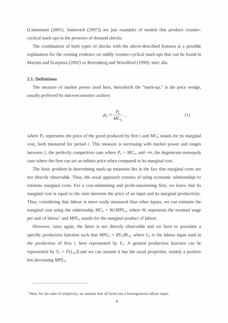
2.1. Definitions

The measure of market power used here, henceforth the “mark-up,” is the price wedge,

usually preferred by macroeconomics authors

itit

it

P

MCµ = , (1)

where Pit represents the price of the good produced by firm i and MCit stands for its marginal

cost, both measured for period t. This measure is increasing with market power and ranges

between 1, the perfectly competitive case where Pit = MCit, and +∞, the degenerate-monopoly

case where the firm can set an infinite price when compared to its marginal cost.

The basic problem in determining mark-up measures lies in the fact that marginal costs are

not directly observable. Thus, the usual approach consists of using economic relationships to

estimate marginal costs. For a cost-minimising and profit-maximising firm, we know that its

marginal cost is equal to the ratio between the price of an input and its marginal productivity.

Thus, considering that labour is more easily measured than other inputs, we can estimate the

marginal cost using the relationship MCit = Wt/MPLit, where Wt represents the nominal wage

per unit of labour1 and MPLit stands for the marginal product of labour.

However, once again, the latter is not directly observable and we have to postulate a

specific production function such that MPLit = ∂Yit/∂Lit, where Lit is the labour input used in

the production of firm i, here represented by Yit. A general production function can be

represented by Yit = F(Lit,⋅) and we can assume it has the usual properties, namely a positive

but decreasing MPLit.

1 Here, for the sake of simplicity, we assume that all firms use a homogeneous labour input.

5

2.2. Average mark-ups

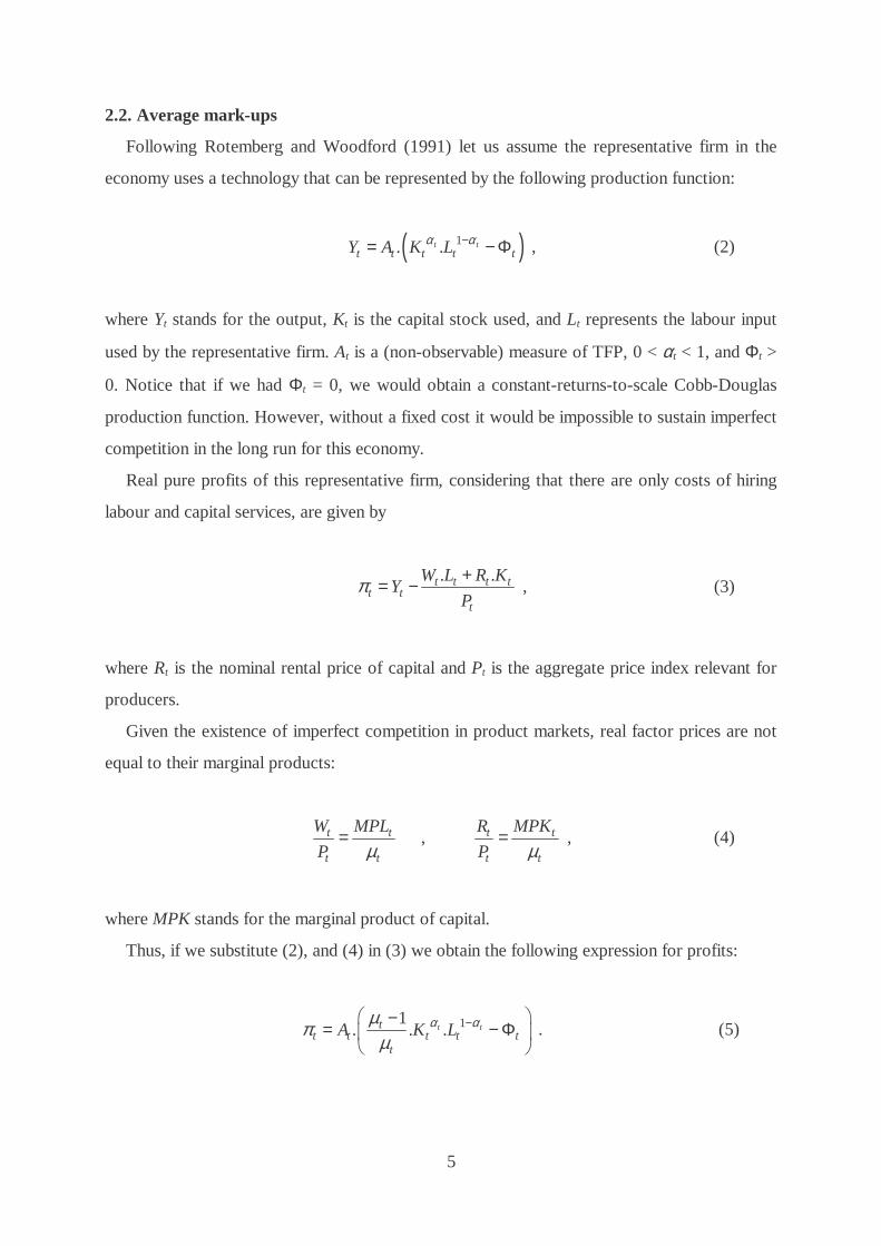
Following Rotemberg and Woodford (1991) let us assume the representative firm in the

economy uses a technology that can be represented by the following production function:

( )1. .t tt t t t tY A K Lα α−= − Φ , (2)

where Yt stands for the output, Kt is the capital stock used, and Lt represents the labour input

used by the representative firm. At is a (non-observable) measure of TFP, 0 < αt < 1, and Φt >

0. Notice that if we had Φt = 0, we would obtain a constant-returns-to-scale Cobb-Douglas

production function. However, without a fixed cost it would be impossible to sustain imperfect

competition in the long run for this economy.

Real pure profits of this representative firm, considering that there are only costs of hiring

labour and capital services, are given by

. .t t t t

t tt

W L R KY

Pπ += − , (3)

where Rt is the nominal rental price of capital and Pt is the aggregate price index relevant for

producers.

Given the existence of imperfect competition in product markets, real factor prices are not

equal to their marginal products:

,t t t t

t t t t

W MPL R MPK

P Pµ µ= = , (4)

where MPK stands for the marginal product of capital.

Thus, if we substitute (2), and (4) in (3) we obtain the following expression for profits:

11. . .t tt

t t t t tt

A K Lα αµπµ

− −= − Φ

. (5)

6

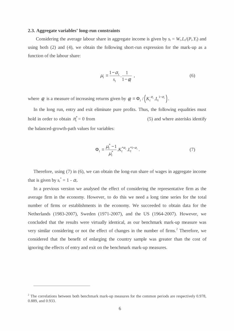
2.3. Aggregate variables’ long-run constraints

Considering the average labour share in aggregate income is given by st = Wt.Lt/(Pt.Yt) and

using both (2) and (4), we obtain the following short-run expression for the mark-up as a

function of the labour share:

1 1

.1

tt

t ts

αµφ

−=−

, (6)

where tφ is a measure of increasing returns given by ( )1/ .t tt t t tK Lα αφ −= Φ .

In the long run, entry and exit eliminate pure profits. Thus, the following equalities must

hold in order to obtain *tπ = 0 from (5) and where asterisks identify

the balanced-growth-path values for variables:

*

1* **

1. .t tt

t t tt

K Lα αµµ

−−Φ = . (7)

Therefore, using (7) in (6), we can obtain the long-run share of wages in aggregate income

that is given by st* = 1 - αt.

In a previous version we analysed the effect of considering the representative firm as the

average firm in the economy. However, to do this we need a long time series for the total

number of firms or establishments in the economy. We succeeded to obtain data for the

Netherlands (1983-2007), Sweden (1971-2007), and the US (1964-2007). However, we

concluded that the results were virtually identical, as our benchmark mark-up measure was

very similar considering or not the effect of changes in the number of firms.2 Therefore, we

considered that the benefit of enlarging the country sample was greater than the cost of

ignoring the effects of entry and exit on the benchmark mark-up measures.

2 The correlations between both benchmark mark-up measures for the common periods are respectively 0.978, 0.889, and 0.933.

7

3. Computing the average mark-up throughout time

3.1. The data

We consider the following OECD countries for which there was data on average mark-ups

for a long recent period (broadly for the period 1970-2007): Belgium, Canada, Denmark,

Finland, France, Germany, Italy, Japan, the Netherlands, Norway, Sweden, the UK, and the

US.

The macroeconomic variables were taken from the European Commission AMECO

database (codes in brackets) and correspond to:

- Yt represents real GDP (1.1.0.0.OVGD) per capita, i.e. per head between 15 and 64 years

old (1.0.0.0.NPAN), measured in 2000 Purchasing Power Standards (PPS).

- Kt stands for real capital stock (1.0.0.0.OKND) per capita, measured in 2000 PPS.

- Lt is total hours worked, i.e. the product of average hours per employee (1.0.0.0.NLHA)

and total employment (1.0.0.0.NETN).

- st represents the adjusted wage share in total income (1.0.0.0.ALCD0).3

For the data on µ*t, i.e. the long-run mark-up ratios for the economy, we used two different

sources of information. We used the information in Martins et al. (1996), Table 3, and

calculated the gross-production-weighted average mark-ups for the period 1980-92 for 14

OECD countries.

3.2. Mark-up time series

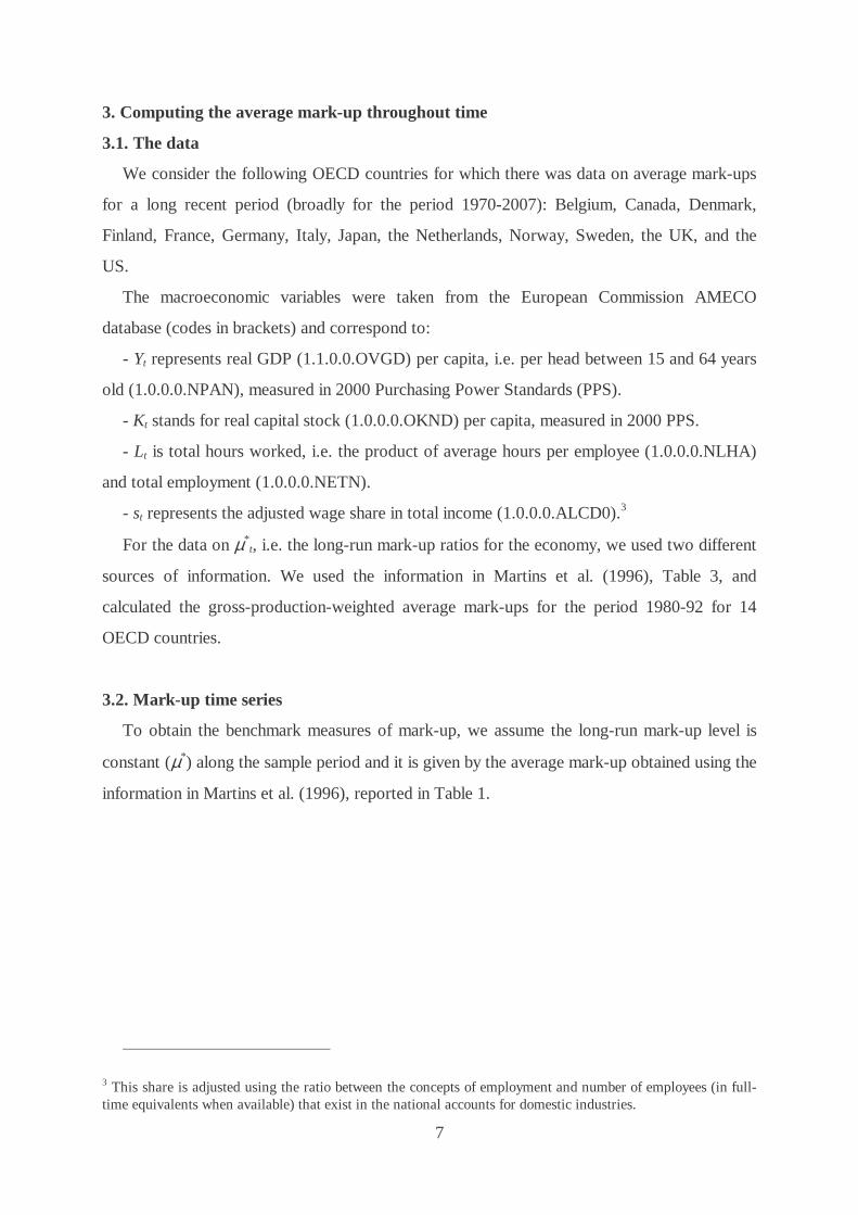
To obtain the benchmark measures of mark-up, we assume the long-run mark-up level is

constant (µ*) along the sample period and it is given by the average mark-up obtained using the

information in Martins et al. (1996), reported in Table 1.

3 This share is adjusted using the ratio between the concepts of employment and number of employees (in full-time equivalents when available) that exist in the national accounts for domestic industries.

8

Table 1 – Production-weighted average mark-ups 1980-1992

Country Average mark-up Australia 1.293 Belgium 1.269 Canada 1.279 Denmark 1.265 Finland 1.252 France 1.263 Germany $ 1.248 Italy 1.376 Japan 1.271 Netherlands 1.262 Norway 1.201 Sweden 1.199 UK 1.232 US 1.203

Source: Martins et al. (1996). NOTE: Sectors considered: Manufacturing; Electricity, Gas, and Water; Construction; Wholesale, Retail Trade, Restaurants, and Hotels (Wholesale and Retail Trade for Australia and Japan); and Transport, Storage, and Communication. Gross-production weights obtained using 1990 data, except for Australia (1989), Belgium, Finland, and Sweden (1995), Italy (1985), and Netherlands (1986). $ - West Germany.

Next, we allow the long-run parameters (αt, Φt) to change smoothly over time. We obtain

the balanced-growth-path series for the pair of parameters using the Hoddrick-Prescott (HP)

filter with λ = 100. The series for αt is simply given by HP(1 - st,100). The series for Φt is

obtained by applying the HP filter to the right-hand side of (7).

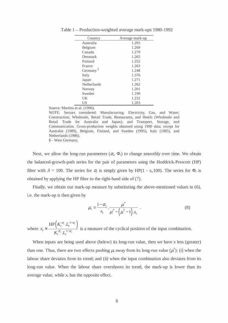
Finally, we obtain our mark-up measure by substituting the above-mentioned values in (6),

i.e. the mark-up is then given by

( )*

* *

1.

1 .t

tt t

s x

α µµµ µ

−=

− − . (8)

where ( )1

1

HP .

.

t t

t t

t tt

t t

K Lx

K L

α α

α α

−

−≡ is a measure of the cyclical position of the input combination.

When inputs are being used above (below) its long-run value, then we have x less (greater)

than one. Thus, there are two effects pushing µt away from its long-run value (µ*): (i) when the

labour share deviates from its trend; and (ii) when the input combination also deviates from its

long-run value. When the labour share overshoots its trend, the mark-up is lower than its

average value, while xt has the opposite effect.

9

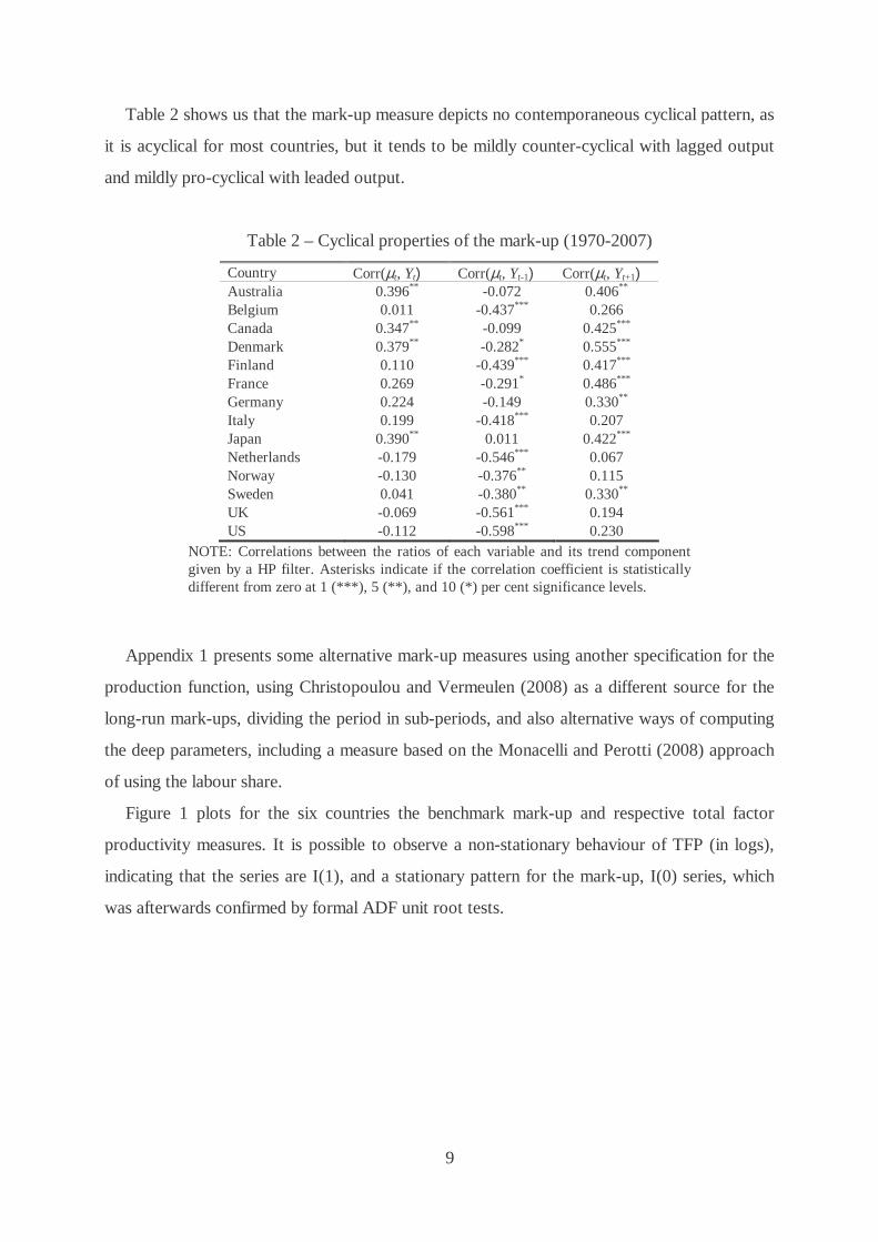
Table 2 shows us that the mark-up measure depicts no contemporaneous cyclical pattern, as

it is acyclical for most countries, but it tends to be mildly counter-cyclical with lagged output

and mildly pro-cyclical with leaded output.

Table 2 – Cyclical properties of the mark-up (1970-2007)

Country Corr(µt, Yt) Corr(µt, Yt-1) Corr(µt, Yt+1) Australia 0.396** -0.072 0.406** Belgium 0.011 -0.437*** 0.266 Canada 0.347** -0.099 0.425*** Denmark 0.379** -0.282* 0.555*** Finland 0.110 -0.439*** 0.417*** France 0.269 -0.291* 0.486*** Germany 0.224 -0.149 0.330** Italy 0.199 -0.418*** 0.207 Japan 0.390** 0.011 0.422*** Netherlands -0.179 -0.546*** 0.067 Norway -0.130 -0.376** 0.115 Sweden 0.041 -0.380** 0.330** UK -0.069 -0.561*** 0.194 US -0.112 -0.598*** 0.230

NOTE: Correlations between the ratios of each variable and its trend component given by a HP filter. Asterisks indicate if the correlation coefficient is statistically different from zero at 1 (***), 5 (**), and 10 (*) per cent significance levels.

Appendix 1 presents some alternative mark-up measures using another specification for the

production function, using Christopoulou and Vermeulen (2008) as a different source for the

long-run mark-ups, dividing the period in sub-periods, and also alternative ways of computing

the deep parameters, including a measure based on the Monacelli and Perotti (2008) approach

of using the labour share.

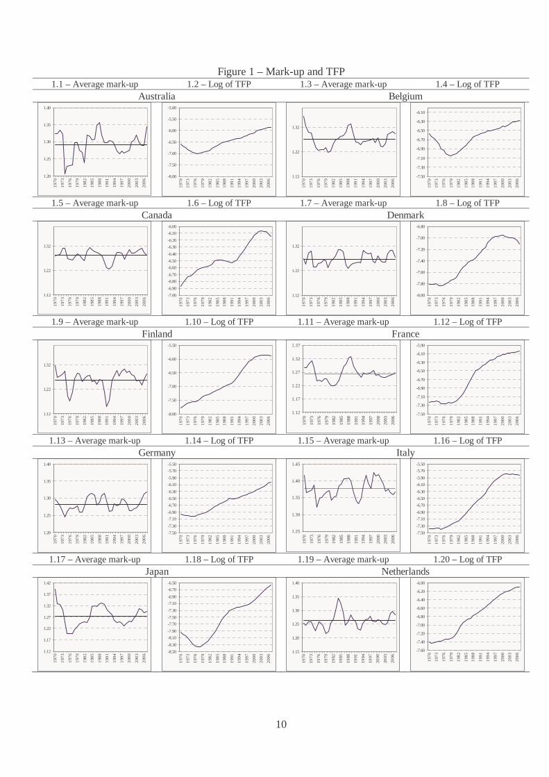
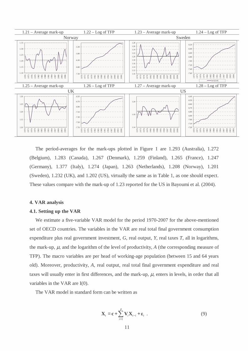
Figure 1 plots for the six countries the benchmark mark-up and respective total factor

productivity measures. It is possible to observe a non-stationary behaviour of TFP (in logs),

indicating that the series are I(1), and a stationary pattern for the mark-up, I(0) series, which

was afterwards confirmed by formal ADF unit root tests.

10

Figure 1 – Mark-up and TFP 1.1 – Average mark-up 1.2 – Log of TFP 1.3 – Average mark-up 1.4 – Log of TFP

Australia Belgium

1.20

1.25

1.30

1.35

1.40

1970

1973

1976

1979

1982

1985

1988

1991

1994

1997

2000

2003

2006

-8.00

-7.50

-7.00

-6.50

-6.00

-5.50

-5.00

1970

1973

1976

1979

1982

1985

1988

1991

1994

1997

2000

2003

2006

1.12

1.22

1.32

1970

1973

1976

1979

1982

1985

1988

1991

1994

1997

2000

2003

2006

-7.50

-7.30

-7.10

-6.90

-6.70

-6.50

-6.30

-6.10

1970

1973

1976

1979

1982

1985

1988

1991

1994

1997

2000

2003

2006

1.5 – Average mark-up 1.6 – Log of TFP 1.7 – Average mark-up 1.8 – Log of TFP

Canada Denmark

1.12

1.22

1.32

197

0

197

3

197

6

197

9

198

2

198

5

198

8

199

1

199

4

199

7

200

0

200

3

200

6

-7.00

-6.90

-6.80

-6.70

-6.60

-6.50

-6.40

-6.30

-6.20

-6.10

-6.00

197

0

197

3

197

6

197

9

198

2

198

5

198

8

199

1

199

4

199

7

200

0

200

3

200

6

1.12

1.22

1.32

197

0

197

3

197

6

197

9

198

2

198

5

198

8

199

1

199

4

199

7

200

0

200

3

200

6

-8.00

-7.80

-7.60

-7.40

-7.20

-7.00

-6.80

197

0

197

3

197

6

197

9

198

2

198

5

198

8

199

1

199

4

199

7

200

0

200

3

200

6


Finland France

1.12

1.22

1.32

197

0

197

3

197

6

197

9

198

2

198

5

198

8

199

1

199

4

199

7

200

0

200

3

200

6

-8.00

-7.50

-7.00

-6.50

-6.00

-5.50

197

0

197

3

197

6

197

9

198

2

198

5

198

8

199

1

199

4

199

7

200

0

200

3

200

6

1.12

1.17

1.22

1.27

1.32

1.37

1970

1973

1976

1979

1982

1985

1988

1991

1994

1997

2000

2003

2006

-7.50

-7.30

-7.10

-6.90

-6.70

-6.50

-6.30

-6.10

-5.90

197

0

197

3

197

6

197

9

198

2

198

5

198

8

199

1

199

4

199

7

200

0

200

3

200

6


Germany Italy

1.20

1.25

1.30

1.35

1.40

197

0

197

3

197

6

197

9

198

2

198

5

198

8

199

1

199

4

199

7

200

0

200

3

200

6

-7.50

-7.30

-7.10

-6.90

-6.70

-6.50

-6.30

-6.10

-5.90

-5.70

-5.50

197

0

197

3

197

6

197

9

198

2

198

5

198

8

199

1

199

4

199

7

200

0

200

3

200

6

1.25

1.30

1.35

1.40

1.45

1970

1973

1976

1979

1982

1985

1988

1991

1994

1997

2000

2003

2006

-7.50

-7.30

-7.10

-6.90

-6.70

-6.50

-6.30

-6.10

-5.90

-5.70

-5.50

197

0

197

3

197

6

197

9

198

2

198

5

198

8

199

1

199

4

199

7

200

0

200

3

200

6


Japan Netherlands

1.12

1.17

1.22

1.27

1.32

1.37

1.42

197

0

197

3

197

6

197

9

198

2

198

5

198

8

199

1

199

4

199

7

200

0

200

3

200

6

-8.50

-8.30

-8.10

-7.90

-7.70

-7.50

-7.30

-7.10

-6.90

-6.70

-6.50

197

0

197

3

197

6

197

9

198

2

198

5

198

8

199

1

199

4

199

7

200

0

200

3

200

6

1.15

1.20

1.25

1.30

1.35

1.40

1970

1973

1976

1979

1982

1985

1988

1991

1994

1997

2000

2003

2006

-7.60

-7.40

-7.20

-7.00

-6.80

-6.60

-6.40

-6.20

-6.00

197

0

197

3

197

6

197

9

198

2

198

5

198

8

199

1

199

4

199

7

200

0

200

3

200

6

11

1.21 – Average mark-up 1.22 – Log of TFP 1.23 – Average mark-up 1.24 – Log of TFP Norway Sweden

1.10

1.15

1.20

1.25

1.30

1.35

1970

1973

1976

1979

1982

1985

1988

1991

1994

1997

2000

2003

2006

-7.30

-6.80

-6.30

-5.80

-5.30

197

0

197

3

197

6

197

9

198

2

198

5

198

8

199

1

199

4

199

7

200

0

200

3

200

6

1.10

1.12

1.14

1.16

1.18

1.20

1.22

1.24

1.26

1.28

1970

1973

1976

1979

1982

1985

1988

1991

1994

1997

2000

2003

2006

-7.60

-7.40

-7.20

-7.00

-6.80

-6.60

-6.40

-6.20

197

0

197

3

197

6

197

9

198

2

198

5

198

8

199

1

199

4

199

7

200

0

200

3

200

6

lnA[A4] 1.25 – Average mark-up 1.26 – Log of TFP 1.27 – Average mark-up 1.28 – Log of TFP

UK US

1.10

1.15

1.20

1.25

1.30

197

0

197

3

197

6

197

9

198

2

198

5

198

8

199

1

199

4

199

7

200

0

200

3

200

6

-7.70

-7.50

-7.30

-7.10

-6.90

-6.70

-6.50

197

0

197

3

197

6

197

9

198

2

198

5

198

8

199

1

199

4

199

7

200

0

200

3

200

6

1.14

1.19

1.24

1970

1973

1976

1979

1982

1985

1988

1991

1994

1997

2000

2003

2006

-7.20

-7.10

-7.00

-6.90

-6.80

-6.70

-6.60

-6.50

-6.40

1970

1973

1976

1979

1982

1985

1988

1991

1994

1997

2000

2003

2006

The period-averages for the mark-ups plotted in Figure 1 are 1.293 (Australia), 1.272

(Belgium), 1.283 (Canada), 1.267 (Denmark), 1.259 (Finland), 1.265 (France), 1.247

(Germany), 1.377 (Italy), 1.274 (Japan), 1.263 (Netherlands), 1.208 (Norway), 1.201

(Sweden), 1.232 (UK), and 1.202 (US), virtually the same as in Table 1, as one should expect.

These values compare with the mark-up of 1.23 reported for the US in Bayoumi et al. (2004).

4. VAR analysis

4.1. Setting up the VAR

We estimate a five-variable VAR model for the period 1970-2007 for the above-mentioned

set of OECD countries. The variables in the VAR are real total final government consumption

expenditure plus real government investment, G, real output, Y, real taxes T, all in logarithms,

the mark-up, µ, and the logarithm of the level of productivity, A (the corresponding measure of

TFP). The macro variables are per head of working-age population (between 15 and 64 years

old). Moreover, productivity, A, real output, real total final government expenditure and real

taxes will usually enter in first differences, and the mark-up, µ, enters in levels, in order that all

variables in the VAR are I(0).

The VAR model in standard form can be written as

1

p

t i t i ti

−=

= + +∑X c V X ε . (9)

12

where Xt denotes the (5 1)× vector of the five endogenous variables given

by [ ] 'ln ln ln lnt t t t t tA G T Y µ≡ ∆ ∆ ∆ ∆X , c is a (5 1)× vector of intercept terms, V is the

matrix of autoregressive coefficients of order (5 5)× , and the vector of random

disturbances'A G T Y

t t t t t tµε ε ε ε ε ≡ ε . The lag length of the endogeneous variables, p,

will be determined by the usual information criteria.

The VAR is ordered from the most exogenous variable to the least exogenous one, with the

log of TFP in the first position. As a result, a shock to productivity may have an instantaneous

effect on all the other variables. However, TFP does not respond contemporaneously to any

structural disturbances to the remaining variables. In the same way, total final government

expenditure also does not react contemporaneously to taxes, to GDP or to the mark-up, due

for instance, to lags in government decision-making. In other words, the mark-up, GDP, taxes,

and final government spending, may affect productivity with a one-period lag. For instance, a

shock in taxes, the third variable, does not have an instantaneous impact on consumption

expenditure of general government or in techonology, but it affects contemporaneously real

output and the mark-up.

In addition to the data used in section three, to compute the average mark-up throughout

time, we now used for the VAR also the following series: total final government consumption

expenditure (1.1.0.0.OCTG), government gross fixed capital formation (1.0.0.0.UIGG), while

government revenues are the sum of direct taxes (1.0.0.0.UTYG), indirect taxes

(1.0.0.0.UTVG), and social security contributions (1.0.0.0.UTSG), divided by the GDP

deflator, which is computed as the ratio between nominal GDP (1.0.0.0.UVGD) and real GDP.

4.2. Estimation and results

Since real output, real total final government consumption expenditure, real output, real

taxes and TFP are I(1) variables, they enter in the VAR in first differences. On the other hand,

the mark-up is a I(0) variable entering therefore in levels in the VAR. The unit root tests

provide similar stationarity results for all countries (see Table 3).

13

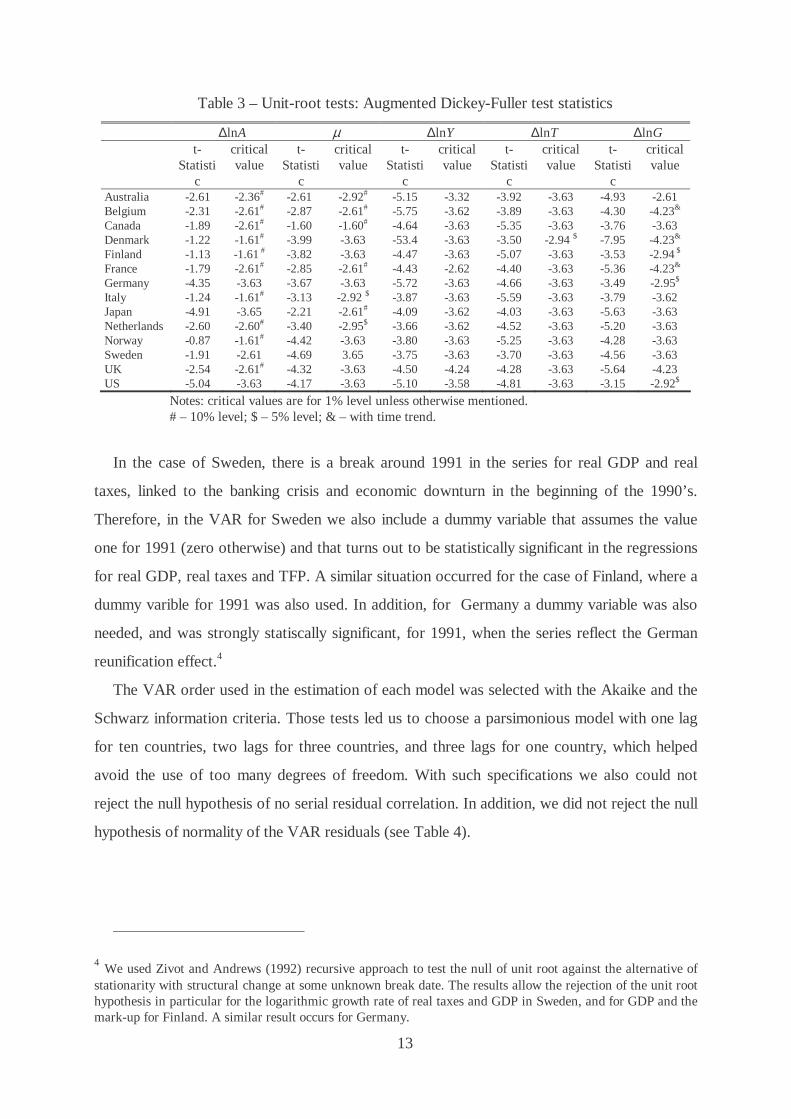
Table 3 – Unit-root tests: Augmented Dickey-Fuller test statistics

∆lnA µ ∆lnY ∆lnT ∆lnG t-

Statistic

critical value

t-Statisti

c

critical value

t-Statisti

c

critical value

t-Statisti

c

critical value

t-Statisti

c

critical value

Australia -2.61 -2.36# -2.61 -2.92# -5.15 -3.32 -3.92 -3.63 -4.93 -2.61 Belgium -2.31 -2.61# -2.87 -2.61# -5.75 -3.62 -3.89 -3.63 -4.30 -4.23& Canada -1.89 -2.61# -1.60 -1.60# -4.64 -3.63 -5.35 -3.63 -3.76 -3.63 Denmark -1.22 -1.61# -3.99 -3.63 -53.4 -3.63 -3.50 -2.94 $ -7.95 -4.23& Finland -1.13 -1.61 # -3.82 -3.63 -4.47 -3.63 -5.07 -3.63 -3.53 -2.94 $ France -1.79 -2.61# -2.85 -2.61# -4.43 -2.62 -4.40 -3.63 -5.36 -4.23& Germany -4.35 -3.63 -3.67 -3.63 -5.72 -3.63 -4.66 -3.63 -3.49 -2.95$ Italy -1.24 -1.61# -3.13 -2.92 $ -3.87 -3.63 -5.59 -3.63 -3.79 -3.62 Japan -4.91 -3.65 -2.21 -2.61# -4.09 -3.62 -4.03 -3.63 -5.63 -3.63 Netherlands -2.60 -2.60# -3.40 -2.95$ -3.66 -3.62 -4.52 -3.63 -5.20 -3.63 Norway -0.87 -1.61# -4.42 -3.63 -3.80 -3.63 -5.25 -3.63 -4.28 -3.63 Sweden -1.91 -2.61 -4.69 3.65 -3.75 -3.63 -3.70 -3.63 -4.56 -3.63 UK -2.54 -2.61# -4.32 -3.63 -4.50 -4.24 -4.28 -3.63 -5.64 -4.23 US -5.04 -3.63 -4.17 -3.63 -5.10 -3.58 -4.81 -3.63 -3.15 -2.92$

Notes: critical values are for 1% level unless otherwise mentioned. # – 10% level; $ – 5% level; & – with time trend.

In the case of Sweden, there is a break around 1991 in the series for real GDP and real

taxes, linked to the banking crisis and economic downturn in the beginning of the 1990’s.

Therefore, in the VAR for Sweden we also include a dummy variable that assumes the value

one for 1991 (zero otherwise) and that turns out to be statistically significant in the regressions

for real GDP, real taxes and TFP. A similar situation occurred for the case of Finland, where a

dummy varible for 1991 was also used. In addition, for Germany a dummy variable was also

needed, and was strongly statiscally significant, for 1991, when the series reflect the German

reunification effect.4

The VAR order used in the estimation of each model was selected with the Akaike and the

Schwarz information criteria. Those tests led us to choose a parsimonious model with one lag

for ten countries, two lags for three countries, and three lags for one country, which helped

avoid the use of too many degrees of freedom. With such specifications we also could not

reject the null hypothesis of no serial residual correlation. In addition, we did not reject the null

hypothesis of normality of the VAR residuals (see Table 4).

4 We used Zivot and Andrews (1992) recursive approach to test the null of unit root against the alternative of stationarity with structural change at some unknown break date. The results allow the rejection of the unit root hypothesis in particular for the logarithmic growth rate of real taxes and GDP in Sweden, and for GDP and the mark-up for Finland. A similar result occurs for Germany.

14

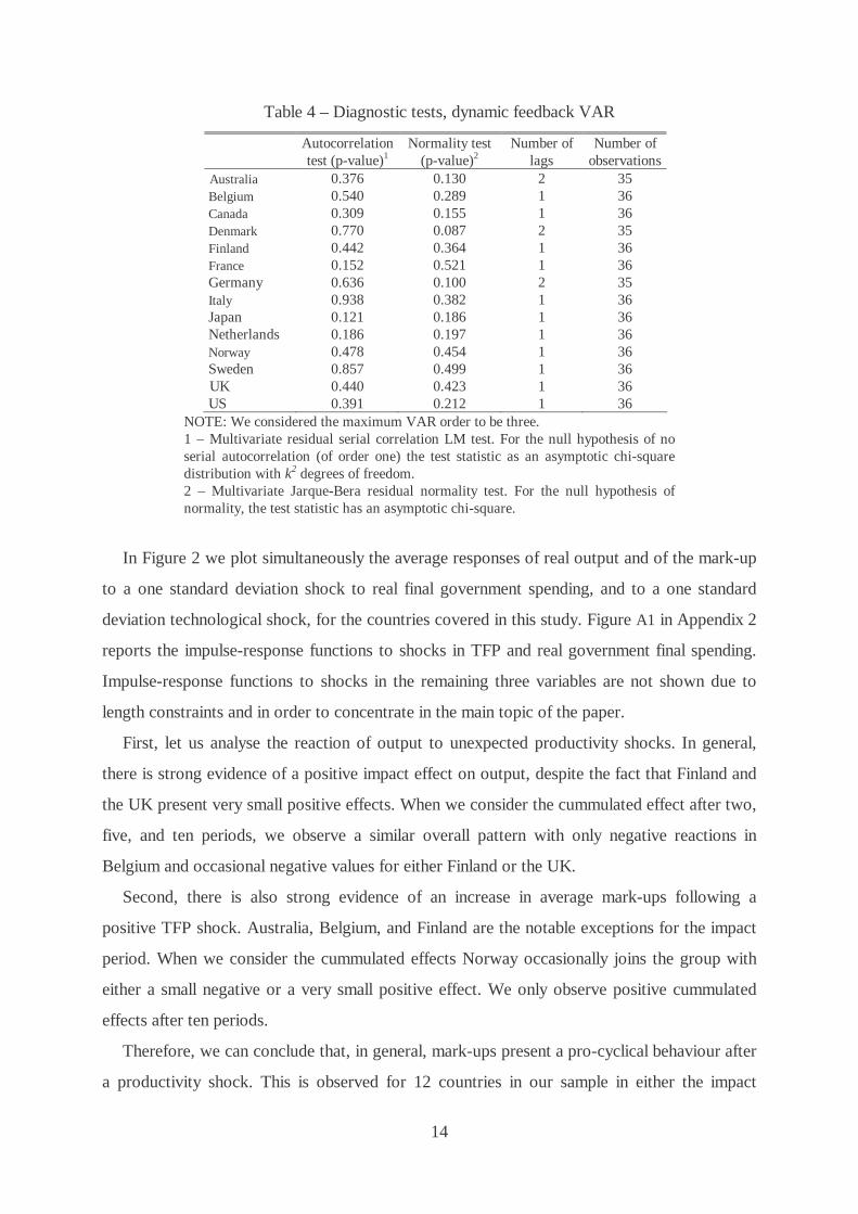
Table 4 – Diagnostic tests, dynamic feedback VAR

Autocorrelation test (p-value)1

Normality test (p-value)2

Number of lags

Number of observations

Australia 0.376 0.130 2 35 Belgium 0.540 0.289 1 36 Canada 0.309 0.155 1 36 Denmark 0.770 0.087 2 35 Finland 0.442 0.364 1 36 France 0.152 0.521 1 36 Germany 0.636 0.100 2 35 Italy 0.938 0.382 1 36 Japan 0.121 0.186 1 36 Netherlands 0.186 0.197 1 36 Norway 0.478 0.454 1 36 Sweden 0.857 0.499 1 36 UK 0.440 0.423 1 36 US 0.391 0.212 1 36

NOTE: We considered the maximum VAR order to be three. 1 – Multivariate residual serial correlation LM test. For the null hypothesis of no serial autocorrelation (of order one) the test statistic as an asymptotic chi-square distribution with k2 degrees of freedom. 2 – Multivariate Jarque-Bera residual normality test. For the null hypothesis of normality, the test statistic has an asymptotic chi-square.

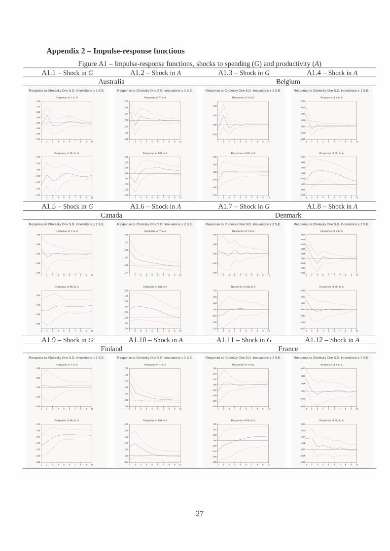
In Figure 2 we plot simultaneously the average responses of real output and of the mark-up

to a one standard deviation shock to real final government spending, and to a one standard

deviation technological shock, for the countries covered in this study. Figure A1 in Appendix 2

reports the impulse-response functions to shocks in TFP and real government final spending.

Impulse-response functions to shocks in the remaining three variables are not shown due to

length constraints and in order to concentrate in the main topic of the paper.

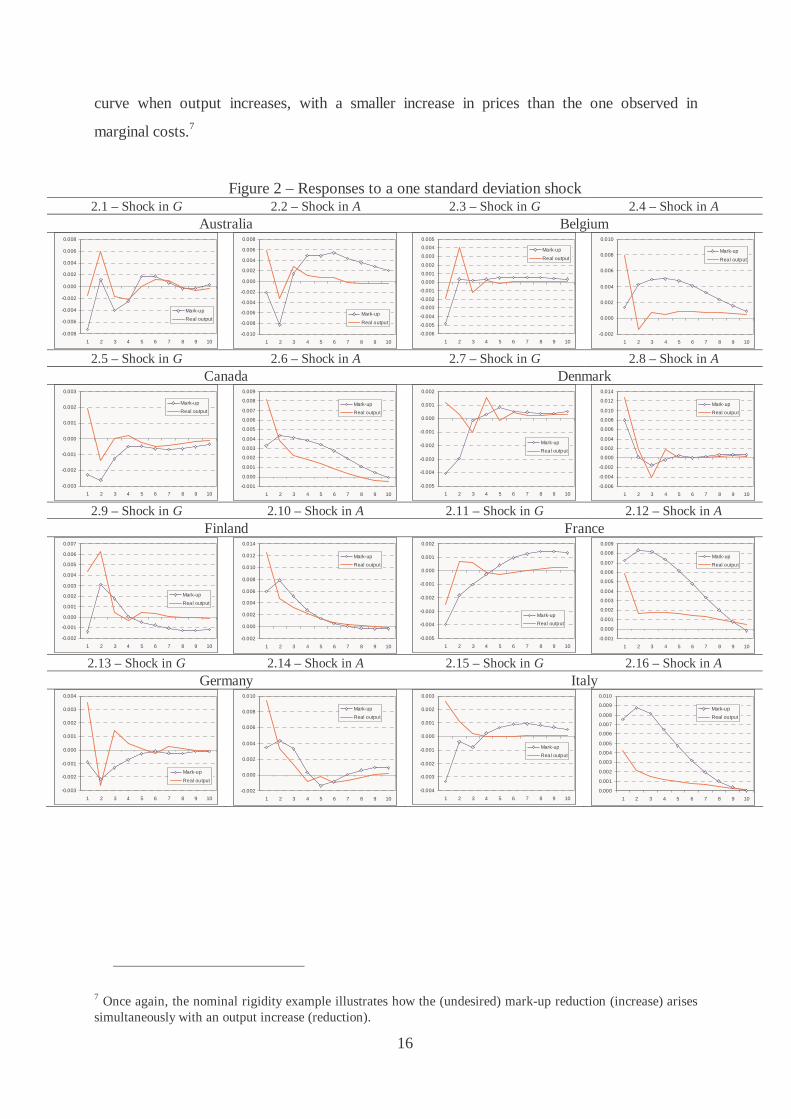
First, let us analyse the reaction of output to unexpected productivity shocks. In general,

there is strong evidence of a positive impact effect on output, despite the fact that Finland and

the UK present very small positive effects. When we consider the cummulated effect after two,

five, and ten periods, we observe a similar overall pattern with only negative reactions in

Belgium and occasional negative values for either Finland or the UK.

Second, there is also strong evidence of an increase in average mark-ups following a

positive TFP shock. Australia, Belgium, and Finland are the notable exceptions for the impact

period. When we consider the cummulated effects Norway occasionally joins the group with

either a small negative or a very small positive effect. We only observe positive cummulated

effects after ten periods.

Therefore, we can conclude that, in general, mark-ups present a pro-cyclical behaviour after

a productivity shock. This is observed for 12 countries in our sample in either the impact

15

period and also considering the cummulated effects after two, five, and ten periods This

outcome is consistent with most endogenous mark-ups hypothesis in the literature, either of

the undesired or of the desired kinds: a productivity shock has a strong direct effect in shifting

the marginal-cost schedule downnwards and a smaller effect moving rightwards along both the

marginal-cost and demand curves when output increases.5

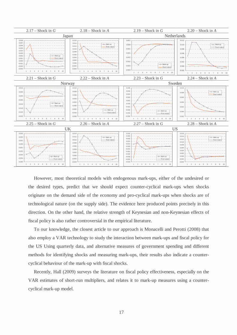
Third, let us observe the effect of an unexpected shock in government final spending on

output. A group of six countries show a considerable short-run (i.e. impact) Keynesian effect:

Belgium, Canada, Finland, Germany, Japan, and Sweden. Italy and the UK present very small

positive reactions of output to a positive fiscal schock of this kind. Australia and Denmark join

the group when we consider the cummulated effects after two, five, and ten periods, but

Germany, Sweden, and the UK leave it. Canada shows a long-run (i.e. considering the first ten

periods cummulated) non-Keynesian effect. France, Netherlands, Norway, and the US also

present evidence consistent with the so-called non-Keynesian effects.6

Fourth, there is strong evidence of a decrease in average mark-ups following a positive

government-spending shock. Sweden and the US are the notable exceptions to this pattern in

the impact period. France, Japan, and the UK occasionaly join the group for larger time

windows, but no more than four countries present simultaneously a positive cummulated effect

on mark-ups.

Thus, we can conclude that, for most countries, mark-ups present a counter-cyclical

behaviour following a government spending shock. This is observed at least for seven countries

in our sample in either the impact period and also considering the cummulated effects after

two, five, and ten periods. Australia, Denmark, France, Netherlands, Norway, and Sweden are

the exceptions in the short run. We can only find evidence of consistent pro-cyclical behaviour

of mark-ups for the Netherlands and Norway. Germany also presents a similar pattern from

period two onwards. Canada, Japan, and the UK also present occasionally less expected

combinations. Again, the results obtained are consistent with existing theoretical endogenous

mark-up models: a government spending shock, or a similar aggregate demand shock, implies

a shift to the right in the demand curve and a rightward movement along the marginal-cost

5 Nominal rigidity provides a good example of a constant or sluggish marginal-revenue curve faced by each producer. 6 Notice that nothing can be said for higher frequencies, especially for quarterly data.

16

curve when output increases, with a smaller increase in prices than the one observed in

marginal costs.7

Figure 2 – Responses to a one standard deviation shock 2.1 – Shock in G 2.2 – Shock in A 2.3 – Shock in G 2.4 – Shock in A

Australia Belgium

-0.008

-0.006

-0.004

-0.002

0.000

0.002

0.004

0.006

0.008

1 2 3 4 5 6 7 8 9 10

Mark-up

Real output

-0.010

-0.008

-0.006

-0.004

-0.002

0.000

0.002

0.004

0.006

0.008

1 2 3 4 5 6 7 8 9 10

Mark-up

Real output

-0.006

-0.005

-0.004

-0.003

-0.002

-0.001

0.000

0.001

0.002

0.003

0.004

0.005

1 2 3 4 5 6 7 8 9 10

Mark-up

Real output

-0.002

0.000

0.002

0.004

0.006

0.008

0.010

1 2 3 4 5 6 7 8 9 10

Mark-up

Real output

2.5 – Shock in G 2.6 – Shock in A 2.7 – Shock in G 2.8 – Shock in A

Canada Denmark

-0.003

-0.002

-0.001

0.000

0.001

0.002

0.003

1 2 3 4 5 6 7 8 9 10

Mark-up

Real output

-0.001

0.000

0.001

0.002

0.003

0.004

0.005

0.006

0.007

0.008

0.009

1 2 3 4 5 6 7 8 9 10

Mark-up

Real output

-0.005

-0.004

-0.003

-0.002

-0.001

0.000

0.001

0.002

1 2 3 4 5 6 7 8 9 10

Mark-up

Real output

-0.006

-0.004

-0.002

0.000

0.002

0.004

0.006

0.008

0.010

0.012

0.014

1 2 3 4 5 6 7 8 9 10

Mark-up

Real output


Finland France

-0.002

-0.001

0.000

0.001

0.002

0.003

0.004

0.005

0.006

0.007

1 2 3 4 5 6 7 8 9 10

Mark-up

Real output

-0.002

0.000

0.002

0.004

0.006

0.008

0.010

0.012

0.014

1 2 3 4 5 6 7 8 9 10

Mark-up

Real output

-0.005

-0.004

-0.003

-0.002

-0.001

0.000

0.001

0.002

1 2 3 4 5 6 7 8 9 10

Mark-up

Real output

-0.001

0.000

0.001

0.002

0.003

0.004

0.005

0.006

0.007

0.008

0.009

1 2 3 4 5 6 7 8 9 10

Mark-up

Real output


Germany Italy

-0.003

-0.002

-0.001

0.000

0.001

0.002

0.003

0.004

1 2 3 4 5 6 7 8 9 10

Mark-up

Real output

-0.002

0.000

0.002

0.004

0.006

0.008

0.010

1 2 3 4 5 6 7 8 9 10

Mark-up

Real output

-0.004

-0.003

-0.002

-0.001

0.000

0.001

0.002

0.003

1 2 3 4 5 6 7 8 9 10

Mark-up

Real output

0.000

0.001

0.002

0.003

0.004

0.005

0.006

0.007

0.008

0.009

0.010

1 2 3 4 5 6 7 8 9 10

Mark-up

Real output

7 Once again, the nominal rigidity example illustrates how the (undesired) mark-up reduction (increase) arises simultaneously with an output increase (reduction).

17

2.17 – Shock in G 2.18 – Shock in A 2.19 – Shock in G 2.20 – Shock in A Japan Netherlands

-0.003

-0.002

-0.001

0.000

0.001

0.002

0.003

0.004

0.005

0.006

0.007

0.008

1 2 3 4 5 6 7 8 9 10

Mark-up

Real output

-0.004

-0.002

0.000

0.002

0.004

0.006

0.008

0.010

0.012

0.014

0.016

1 2 3 4 5 6 7 8 9 10

Mark-up

Real output

-0.003

-0.003

-0.002

-0.002

-0.001

-0.001

0.000

0.001

1 2 3 4 5 6 7 8 9 10

Mark-up

Real output

-0.002

0.000

0.002

0.004

0.006

0.008

0.010

0.012

1 2 3 4 5 6 7 8 9 10

Mark-up

Real output

2.21 – Shock in G 2.22 – Shock in A 2.23 – Shock in G 2.24 – Shock in A Norway Sweden

-0.025

-0.020

-0.015

-0.010

-0.005

0.000

0.005

0.010

1 2 3 4 5 6 7 8 9 10

Mark-up

Real output

-0.006

-0.004

-0.002

0.000

0.002

0.004

0.006

0.008

0.010

1 2 3 4 5 6 7 8 9 10

Mark-up

Real output

-0.004

-0.003

-0.002

-0.001

0.000

0.001

0.002

0.003

0.004

0.005

1 2 3 4 5 6 7 8 9 10

Mark-up

Real output

-0.002

0.000

0.002

0.004

0.006

0.008

0.010

1 2 3 4 5 6 7 8 9 10

Mark-up

Real output


UK US

-0.005

-0.004

-0.003

-0.002

-0.001

0.000

0.001

0.002

0.003

1 2 3 4 5 6 7 8 9 10

Mark-up

Real output

-0.004

-0.002

0.000

0.002

0.004

0.006

0.008

0.010

0.012

0.014

1 2 3 4 5 6 7 8 9 10

Mark-up

Real output

-0.003

-0.003

-0.002

-0.002

-0.001

-0.001

0.000

0.001

0.001

0.002

0.002

0.003

1 2 3 4 5 6 7 8 9 10

Mark-up

Real output

-0.004

-0.002

0.000

0.002

0.004

0.006

0.008

0.010

0.012

0.014

0.016

1 2 3 4 5 6 7 8 9 10

Mark-up

Real output

However, most theoretical models with endogenous mark-ups, either of the undesired or

the desired types, predict that we should expect counter-cyclical mark-ups when shocks

originate on the demand side of the economy and pro-cyclical mark-ups when shocks are of

technological nature (on the supply side). The evidence here produced points precisely in this

direction. On the other hand, the relative strength of Keynesian and non-Keynesian effects of

fiscal policy is also rather controversial in the empirical literature.

To our knowledge, the closest article to our approach is Monacelli and Perotti (2008) that

also employ a VAR technology to study the interaction between mark-ups and fiscal policy for

the US Using quarterly data, and alternative measures of government spending and different

methods for identifying shocks and measuring mark-ups, their results also indicate a counter-

cyclical behaviour of the mark-up with fiscal shocks.

Recently, Hall (2009) surveys the literature on fiscal policy effectiveness, especially on the

VAR estimates of short-run multipliers, and relates it to mark-up measures using a counter-

cyclical mark-up model.

18

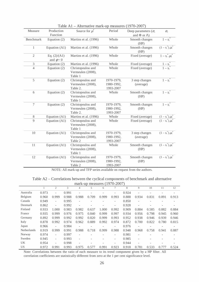
4.3. Robustness

Using alternative mark-up measures and the corresponding TFP measures in the VAR

analysis provided similar results. This should not be a surprise if one takes into account the

high correlations between the alternative and the benchmark measures, once we de-trend them

(see Table A2 in Appendix 1).

Despite the fact that most qualitative results hold for most countries, there are some

quantitative differences and some indications that using one type of mark-up and TFP

measures may be crucial to the outcomes. Further investigation is needed in this front.

In addition, we also estimated the VAR models using first differences of the level of the

variables, instead of logarithmic differences, but the results were broadly similar.

Finally, and in order to allow for the interaction of interest rates, we replicated as an

example the VAR analysis for the US, using either short-term or long-term interest rates. The

results did not change.

4.4. Multipliers and mark-ups in the long run

One of the central issues in the early New Keynesian literature is the relationship between

fiscal-policy effectiveness and market power in the long run – see, inter alia, Costa (2007). We

can use the VAR estimates to obtain long-run elasticities of output to government final

spending:

( )

( )

10

110

1

lnˆ

ln

Git it

ti

Git it

t

X

G

εη

ε=

=

∆=

∆

∑

∑, (10)

where ( )ln Git itX ε∆ represents the effect, given by the impulse-response function, of an

unexpected shock to government final spending on variable X for country i in period t.

The long-run multiplier is obtained dividing iη by the share of government final spending in

GDP. The estimates for the multiplier are presented in Table 5.

19

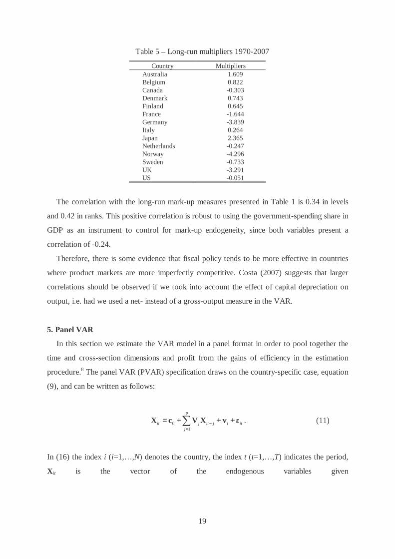
Table 5 – Long-run multipliers 1970-2007

Country Multipliers Australia 1.609 Belgium 0.822 Canada -0.303 Denmark 0.743 Finland 0.645 France -1.644 Germany -3.839 Italy 0.264 Japan 2.365 Netherlands -0.247 Norway -4.296 Sweden -0.733 UK -3.291 US -0.051

The correlation with the long-run mark-up measures presented in Table 1 is 0.34 in levels

and 0.42 in ranks. This positive correlation is robust to using the government-spending share in

GDP as an instrument to control for mark-up endogeneity, since both variables present a

correlation of -0.24.

Therefore, there is some evidence that fiscal policy tends to be more effective in countries

where product markets are more imperfectly competitive. Costa (2007) suggests that larger

correlations should be observed if we took into account the effect of capital depreciation on

output, i.e. had we used a net- instead of a gross-output measure in the VAR.

5. Panel VAR

In this section we estimate the VAR model in a panel format in order to pool together the

time and cross-section dimensions and profit from the gains of efficiency in the estimation

procedure.8 The panel VAR (PVAR) specification draws on the country-specific case, equation

(9), and can be written as follows:

01

p

it j it j i itj

−=

= + + +∑X c V X v ε . (11)

In (16) the index i (i=1,…,N) denotes the country, the index t (t=1,…,T) indicates the period,

Xit is the vector of the endogenous variables given

20

by [ ] 'ln ln ln lnit it it it it itA G T Y µ≡ ∆ ∆ ∆ ∆X , c0 is a vector of intercept terms, V is the

matrix of autoregressive coefficients, vi is the matrix of country-specific fixed effects, and the

vector of random disturbances'A G T Y

it it it it it itµε ε ε ε ε ≡ ε . The lag length of the

endogeneous variables, p, will be set in this case to one, based also on the previously

uncovered country-specific VAR evidence. Since our time dimension is not that small, the use

of time dummies would imply a loss of efficency.

The PVAR allows treating all variables as jointly endogenously, with each variable

depending on its past information and on the realizations of the other variables. In addition the

use of the panel VAR approach increases the degrees of freedom for the estimation. On the

other hand, the PVAR set-up imposes a similar lag structure across all the countries.

Nevertheless, cross-section heterogeneity can be accounted for via the fixed effects, an the bias

due to the existence of lagged endogenous variables can be overcome by using GMM.9

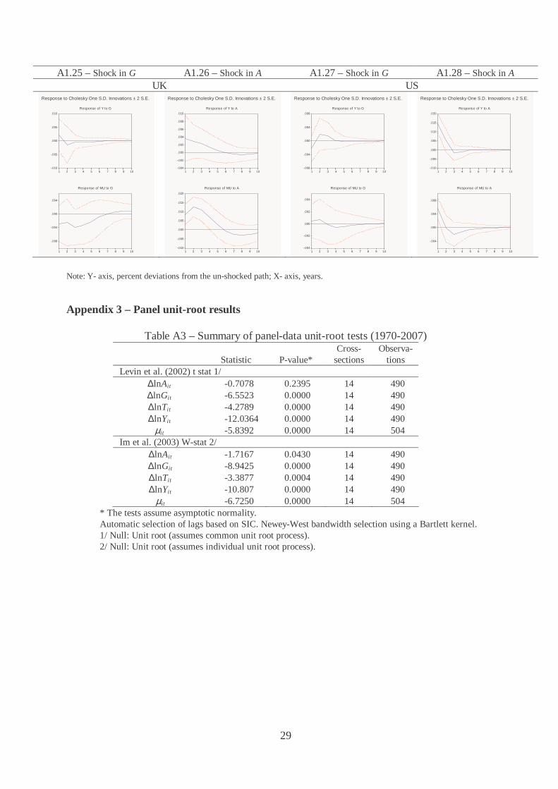
We also checked for the existence of unit roots in the panel using the panel data integration

tests of Im et al. (2003) and Levin et al. (2002), which assume cross-sectional independence

among panel units (except for common time effects). Concerning the first difference of TFP,

government spending, revenues, and GDP, the results given by the panel data unit root tests

(reported in Appendix 3) essentially reveal that the null unit root hypothesis can be rejected.

The same is true for the level of the mark-up, which overall confirms the same integration

order for the variables in the panel as well as in the country-specific analysis.

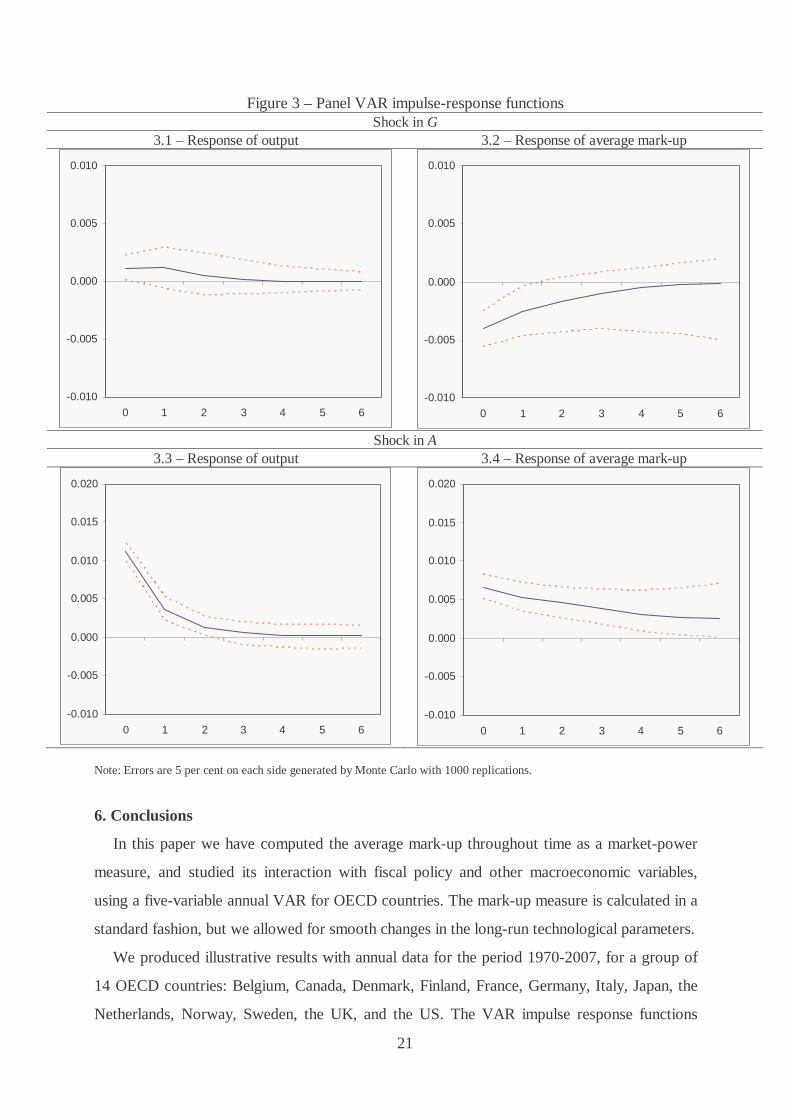
The results of the PVAR impulse response functions are presented in Figure 3. Accordingly,

we can observe a pro-cyclical behaviour of the mark-up with total factor productivity shocks,

and a counter-cyclical behaviour of the mark-up with fiscal spending shocks. Such results

confirm the overall picture that was uncovered with the country-specific VAR evidence.

8 For instance, Beetsma et al. (2008) also use a panel VAR approach in a related context for fiscal and external imbalances. 9 In our computations we use the programs from Love and Zicchino (2006), which include a routine for the removal of the fixed effects via the Helmert transformation and uses GMM to estimate the system OLS.

21

Figure 3 – Panel VAR impulse-response functions Shock in G

3.1 – Response of output 3.2 – Response of average mark-up

-0.010

-0.005

0.000

0.005

0.010

0 1 2 3 4 5 6

-0.010

-0.005

0.000

0.005

0.010

0 1 2 3 4 5 6

Shock in A 3.3 – Response of output 3.4 – Response of average mark-up

-0.010

-0.005

0.000

0.005

0.010

0.015

0.020

0 1 2 3 4 5 6

-0.010

-0.005

0.000

0.005

0.010

0.015

0.020

0 1 2 3 4 5 6

Note: Errors are 5 per cent on each side generated by Monte Carlo with 1000 replications.

6. Conclusions

In this paper we have computed the average mark-up throughout time as a market-power

measure, and studied its interaction with fiscal policy and other macroeconomic variables,

using a five-variable annual VAR for OECD countries. The mark-up measure is calculated in a

standard fashion, but we allowed for smooth changes in the long-run technological parameters.

We produced illustrative results with annual data for the period 1970-2007, for a group of

14 OECD countries: Belgium, Canada, Denmark, Finland, France, Germany, Italy, Japan, the

Netherlands, Norway, Sweden, the UK, and the US. The VAR impulse response functions

22

show that, in general the mark-up (i) depicts a pro-cyclical behaviour with productivity shocks

and (ii) a mildly counter-cyclical behaviour with fiscal spending shocks. Furthermore, we also

obtain non-Keynesian impacts of real final government spending on output in some cases.

Finally, we also used a Panel Vector Auto-Regression analysis, increasing the efficiency in

the estimations, which overall confirmed the country-specific results regarding the behaviour of

the mark-up.

From a policy point of view, positive productivity shocks imply, by its nature, a rightward

shift in labour demand, but an increased mark-up weakens the initial expansive effect on both

employment (and output) and real wages. On the other hand, positive fiscal shocks show,

besides their usual wealth effect via future taxes expanding the labour supply, an additional

effect due to a decrease in the mark-up that shifts the labour demand rightwards, stimulating

further employment (and output) and also real wages. Our results, illustrating the counter-

cyclical behaviour of the mark-up with fiscal spending shocks, imply a stronger effectiveness of

fiscal policy on output and this is especially relevant when the fiscal multiplier is positive.

References

Barro, R. and Tenreyro, S. (2006). Closed and Open Economy Models of Business Cycles

with Marked Up and Sticky Prices. Economic Journal 116(511), 434-456.

Bayoumi, T., Laxton, D. and Pesenti, P. (2004). Benefits and Spillovers of Greater

Competition in Europe: A macroeconomic assessment. NBER Working Papers 10416.

Beetsma, R., Giuliodori, M. and Klaassen, F. (2008). The Effects of Public Spending Shocks

on Trade Balances and Budget Deficits in The European Union. Journal of the European

Economic Association 6(2-3), 414-423.

Bilbiie, J., Ghironi, F. and Melitz, M. (2007). Endogenous Entry, Product Variety, and

Business Cycles. NBER Working Paper 13646.

Christopoulou, R. and Vermeulen, P. (2008). Markups in the Euro Area and the US over the

Period 1981-2004. ECB Working Paper Series 856.

Clarida, R., Galí, J. and Gertler, M. (1999). The Science of Monetary Policy: A New

Keynesian Perspective. Journal of Economic Literature 37, 1661-1707.

Costa, L. (2004). Endogenous Markups and Fiscal Policy. Manchester School 72(S), 55-71.

Costa, L. (2007). GDP Steady-state Multipliers under Imperfect Competition Revisited.

Portuguese Economic Journal 6(3), 181-204.

23

Costa, L. and Dixon, H. (2009). Fiscal Policy under Imperfect Competition: A survey.

ISEG/TULisbon Department of Economics Working Papers 25.

dos Santos Ferreira, R. and Dufourt, F. (2006). Free Entry and Business Cycles under the

Influence of Animal Spirits. Journal of Monetary Economics 53(2), 311-328.

dos Santos Ferreira, R. and Lloyd-Braga, T. (2005). Non-Linear Endogenous Fluctuations

with Free Entry and Variable Markups. Journal of Economic Dynamics and Control 29(5),

847-871.

Feenstra, R. (2003). A Homothetic Utility Function for Monopolistic Competition Models,

without Constant Price Elasticity. Economics Letters 78(1), 79-86.

Galí, J. (1994a). Monopolistic Competition, Business Cycles, and the Composition of

Aggregate Demand. Journal of Economic Theory 63(1), 73-96.

Galí, J. (1994b). Monopolistic Competition, Endogenous Markups, and Growth. European

Economic Review 38(3-4), 748-756.

Goodfriend, M. and King, R. (1997). The New Neo-Classical Synthesis and the Role of

Monetary Policy. NBER Macroeconomics Annual 231-283.

Hairault, J.-O. and Portier, F. (1993). Money, New-Keynesian Macroeconomics and the

Business Cycle. European Economic Review 37(8), 1533-1568.

Hall, R. (1988). The Relationship between Price and Marginal Cost in U.S. Industry. Journal

of Political Economy 96(2), 921-947.

Hall, R. (2009). By How Much Does GDP Rise If the Government Buys More Output? NBER

Working Papers 15496.

Im, K., Pesaran, M. and Shin, Y. (2003). Testing for Unit Roots in Heterogeneous Panels.

Journal of Econometrics 115(1), 53-74.

Jaimovich, N. (2007). Firm Dynamics and Markup Variations: Implications for sunspot

equilibria and endogenous economic fluctuations. Journal of Economic Theory 137(1),

300-325.

Jaimovich, N. and Floetotto, M. (2008). Firm Dynamics, Markup Variations, and the Business

Cycle. Journal of Monetary Economics 55(7), 1238-1252.

Levin, A., Lin, C.-F. and Chu, C.-S. (2002). Unit Root Tests in Panel Data: Asymptotic and

finite sample properties. Journal of Econometrics 108(1), 1-24.

24

Linnemann, L. (2001). The Price Index Effect, Entry, and Endogenous Markups in a

Macroeconomic Model of Monopolistic Competition. Journal of Macroeconomics 23(3),

441-458.

Linnemann, L. and Schabert, A. (2003). Fiscal Policy in the New Neoclassical Synthesis.

Journal of Money, Credit, and Banking 35(6), 911-929.

Love, I. and Zicchino, L. (2006). Financial Development and Dynamic Investment Behavior:

Evidence from panel VAR. Quarterly Review of Economics and Finance 46(2), 190-210.

Martins, J., Scarpetta, S. and Pilat, D. (1996). Mark-up Pricing, Market Structure and the

Business Cycle. OECD Economic Studies 27, 71-105.

Martins, J.O. and Scarpetta, S. (2002). Estimation of the Cyclical Behaviour of Mark-ups: A

technical note. OECD Economic Studies 34(1), 173-188.

Monacelli, T. and Perotti, R. (2008). Fiscal Policy, Wealth Effects, and Markups. NBER

Working Paper 14584.

Portier, F. (1995). Business Formation and Cyclical Markups in the French Business Cycle.

Annales d'Economie et de Statistique 37/38, 411-440.

Ravn, M., Schmitt-Grohé, S. and Uribe, M. (2006). Deep Habits. Review of Economic Studies

73(19), 195-218.

Ravn, M., Schmitt-Grohé, S. and Uribe, M. (2008). Macroeconomics of Subsistence Points.

Macroeconomic Dynamics 12(Suppl. 1), 136-147.

Roeger, W. (1995). Can Imperfect Competition Explain the Difference Between Primal and

Dual Productivity Measures? Estimates for U.S. manufacturing. Journal of Political

Economy 103(2), 316-330.

Rotemberg, J. and Woodford, M. (1991). Markups and the Business Cycle. NBER

Macroeconomics Annual 6 63-128.

Rotemberg, J. and Woodford, M. (1992). Oligopolistic Pricing and the Effects of Aggregate

Demand on Economic Activity. Journal of Political Economy 100(6), 1153-1207.

Rotemberg, J. and Woodford, M. (1995). Dynamic General Equilibrium Models with

Imperfectly Competitive Product Markets. In: Cooley, T., (Ed.) Frontiers of Business

Cycles Research, Princeton University Press, Princeton, pp. pp. 243-330.

Rotemberg, J. and Woodford, M. (1999). The Cyclical Behavior of Prices and Costs. In:

Taylor, J. and Woodford, M., (Eds.) Handbook of Macroeconomics, Elsevier, Amsterdam,

pp. pp. 1051-1135.

25

Zivot, E. and Andrews, D. (1992). Further Evidence on the Great Crash, the Oil-Price Shock,

and the Unit-Root Hypothesis. Journal of Business and Economic Statistics 10(3), 251-

270.

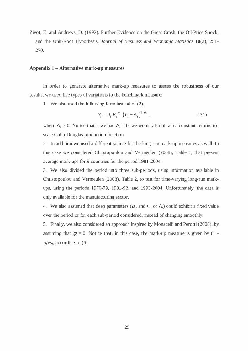
Appendix 1 – Alternative mark-up measures

In order to generate alternative mark-up measures to assess the robustness of our

results, we used five types of variations to the benchmark measure:

1. We also used the following form instead of (2),

( )1. . ttt t t t tY A K L

αα −= − Λ , (A1)

where Λt > 0. Notice that if we had Λt = 0, we would also obtain a constant-returns-to-

scale Cobb-Douglas production function.

2. In addition we used a different source for the long-run mark-up measures as well. In

this case we considered Christopoulou and Vermeulen (2008), Table 1, that present

average mark-ups for 9 countries for the period 1981-2004.

3. We also divided the period into three sub-periods, using information available in

Christopoulou and Vermeulen (2008), Table 2, to test for time-varying long-run mark-

ups, using the periods 1970-79, 1981-92, and 1993-2004. Unfortunately, the data is

only available for the manufacturing sector.

4. We also assumed that deep parameters (αt, and Φt or Λt) could exhibit a fixed value

over the period or for each sub-period considered, instead of changing smoothly.

5. Finally, we also considered an approach inspired by Monacelli and Perotti (2008), by

assuming that φt = 0. Notice that, in this case, the mark-up measure is given by (1 -

αt)/st, according to (6).

26

Table A1 – Alternative mark-up measures (1970-2007) Measure Production

Function Source for µ* Period Deep parameters (α,

and Φ or Λ) αt

Benchmark Equation (2) Martins et al. (1996) Whole Smooth changes (HP)

1 – st*

1 Equation (A1) Martins et al. (1996) Whole Smooth changes (HP)

(1 – st*).µt

*

2 Eq. (2)/(A1) and φ = 0

Martins et al. (1996) Whole Fixed (average) 1 – st*.µt

*

3 Equation (2) Martins et al. (1996) Whole Fixed (average) 1 – st*

4 Equation (2) Christopoulou and Vermeulen (2008), Table 1

Whole Fixed (average) 1 – st*

5 Equation (2) Christopoulou and Vermeulen (2008), Table 2.

1970-1979, 1980-1992, 1993-2007

3 step changes (average)

1 – st*

6 Equation (2) Christopoulou and Vermeulen (2008), Table 1

Whole Smooth changes (HP)

1 – st*

7 Equation (2) Christopoulou and Vermeulen (2008), Table 2.

1970-1979, 1980-1992, 1993-2007

Smooth changes (HP)

1 – st*

8 Equation (A1) Martins et al. (1996) Whole Fixed (average) (1 – st*).µt

* 9 Equation (A1) Christopoulou and

Vermeulen (2008), Table 1

Whole Fixed (average) (1 – st*).µt

*

10 Equation (A1) Christopoulou and Vermeulen (2008), Table 2

1970-1979, 1980-1992, 1993-2007

3 step changes (average)

(1 – st*).µt

*


Whole Smooth changes (HP)

(1 – st*).µt

*


1970-1979, 1980-1992, 1993-2007

Smooth changes (HP)

(1 – st*).µt

*

NOTE: All mark-up and TFP series available on request from the authors.

Table A2 – Correlations between the cyclical components of benchmark and alternative mark-up measures (1970-2007)

1 2 3 4 5 6 7 8 9 10 11 12

Australia 0.973 - 0.991 - - - - 0.924 - - - - Belgium 0.960 0.999 0.988 0.988 0.709 0.999 0.993 0.888 0.934 0.831 0.891 0.913 Canada 0.949 - 0.995 - - - - 0.850 - - - - Denmark 0.862 - 0.992 - - - - 0.928 - - - - Finland 0.933 1.000 0.983 0.982 0.637 1.000 0.992 0.909 0.884 0.585 0.882 0.884 France 0.935 0.999 0.976 0.975 0.840 0.999 0.997 0.934 0.956 0.798 0.945 0.960 Germany 0.892 0.999 0.992 0.992 0.820 0.999 0.993 0.952 0.938 0.946 0.939 0.946 Italy 0.878 0.992 0.974 0.962 0.889 0.992 0.974 0.872 0.700 0.822 0.780 0.815 Japan 0.966 - 0.984 - - - - 0.976 - - - - Netherlands 0.919 0.999 0.991 0.988 0.718 0.999 0.988 0.948 0.968 0.758 0.941 0.887 Norway 0.974 - 0.997 - - - - 0.981 - - - - Sweden 0.945 - 0.993 - - - - 0.985 - - - - UK 0.954 - 0.998 - - - - 0.944 - - - - US 0.972 0.991 0.993 0.975 0.577 0.991 0.923 0.918 0.781 0.533 0.777 0.524

Note: Correlations between the ratio of each measure to its trend component given by a HP filter. All correlation coefficients are statistically different from zero at the 1 per cent significance level.

27

Appendix 2 – Impulse-response functions

Figure A1 – Impulse-response functions, shocks to spending (G) and productivity (A) A1.1 – Shock in G A1.2 – Shock in A A1.3 – Shock in G A1.4 – Shock in A

Australia Belgium

-.012

-.008

-.004

.000

.004

.008

.012

.016

1 2 3 4 5 6 7 8 9 10

Response of Y to G

-.015

-.010

-.005

.000

.005

.010

.015

1 2 3 4 5 6 7 8 9 10

Response of MU to G

Response to Cholesky One S.D. Innovations ± 2 S.E.

-.012

-.008

-.004

.000

.004

.008

.012

1 2 3 4 5 6 7 8 9 10

Response of Y to A

-.020

-.015

-.010

-.005

.000

.005

.010

.015

1 2 3 4 5 6 7 8 9 10

Response of MU to A


-.004

.000

.004

.008

1 2 3 4 5 6 7 8 9 10

Response of Y to G

-.012

-.008

-.004

.000

.004

.008

1 2 3 4 5 6 7 8 9 10

Response of MU to G


-.008

-.004

.000

.004

.008

.012

.016

1 2 3 4 5 6 7 8 9 10

Response of Y to A

-.004

-.002

.000

.002

.004

.006

.008

.010

1 2 3 4 5 6 7 8 9 10

Response of MU to A


A1.5 – Shock in G A1.6 – Shock in A A1.7 – Shock in G A1.8 – Shock in A

Canada Denmark

-.008

-.004

.000

.004

.008

1 2 3 4 5 6 7 8 9 10

Response of Y to G

-.008

-.004

.000

.004

1 2 3 4 5 6 7 8 9 10

Response of MU to G


-.004

.000

.004

.008

.012

.016

1 2 3 4 5 6 7 8 9 10

Response of Y to A

-.004

-.002

.000

.002

.004

.006

.008

.010

1 2 3 4 5 6 7 8 9 10

Response of MU to A


-.008

-.004

.000

.004

.008

1 2 3 4 5 6 7 8 9 10

Response of Y to G

-.012

-.008

-.004

.000

.004

.008

.012

1 2 3 4 5 6 7 8 9 10

Response of MU to G


-.012

-.008

-.004

.000

.004

.008

.012

.016

.020

1 2 3 4 5 6 7 8 9 10

Response of Y to A

-.015

-.010

-.005

.000

.005

.010

.015

1 2 3 4 5 6 7 8 9 10

Response of MU to A



Finland France

-.008

-.004

.000

.004

.008

1 2 3 4 5 6 7 8 9 10

Response of Y to G

-.020

-.015

-.010

-.005

.000

.005

.010

1 2 3 4 5 6 7 8 9 10

Response of MU to G


-.004

.000

.004

.008

.012

.016

.020

1 2 3 4 5 6 7 8 9 10

Response of Y to A

-.004

.000

.004

.008

.012

.016

.020

1 2 3 4 5 6 7 8 9 10

Response of MU to A


-.008

-.006

-.004

-.002

.000

.002

.004

.006

1 2 3 4 5 6 7 8 9 10

Response of Y to G

-.008

-.006

-.004

-.002

.000

.002

.004

.006

1 2 3 4 5 6 7 8 9 10

Response of MU to G


-.008

-.004

.000

.004

.008

.012

1 2 3 4 5 6 7 8 9 10

Response of Y to A

-.008

-.004

.000

.004

.008

.012

.016

1 2 3 4 5 6 7 8 9 10

Response of MU to A


28

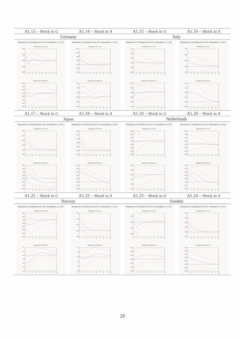
A1.13 – Shock in G A1.14 – Shock in A A1.15 – Shock in G A1.16 – Shock in A Germany Italy

-.008

-.004

.000

.004

.008

1 2 3 4 5 6 7 8 9 10

Response of Y to G

-.008

-.006

-.004

-.002

.000

.002

.004

.006

1 2 3 4 5 6 7 8 9 10

Response of MU to G


-.008

-.004

.000

.004

.008

.012

.016

1 2 3 4 5 6 7 8 9 10

Response of Y to A

-.008

-.004

.000

.004

.008

.012

1 2 3 4 5 6 7 8 9 10

Response of MU to A


-.008

-.004

.000

.004

.008

.012

1 2 3 4 5 6 7 8 9 10

Response of Y to G

-.012

-.008

-.004

.000

.004

.008

1 2 3 4 5 6 7 8 9 10

Response of MU to G


-.004

.000

.004

.008

.012

1 2 3 4 5 6 7 8 9 10

Response of Y to A

-.004

.000

.004

.008

.012

.016

1 2 3 4 5 6 7 8 9 10

Response of MU to A



Japan Netherlands

-.004

.000

.004

.008

.012

.016

1 2 3 4 5 6 7 8 9 10

Response of Y to G

-.006

-.004

-.002

.000

.002

.004

.006

.008

1 2 3 4 5 6 7 8 9 10

Response of MU to G


-.004

.000

.004

.008

.012

.016

.020

1 2 3 4 5 6 7 8 9 10

Response of Y to A

-.008

-.004

.000

.004

.008

.012

.016

.020

1 2 3 4 5 6 7 8 9 10

Response of MU to A


-.008

-.006

-.004

-.002

.000

.002

.004

.006

1 2 3 4 5 6 7 8 9 10

Response of Y to G

-.012

-.008

-.004

.000

.004

.008

1 2 3 4 5 6 7 8 9 10

Response of MU to G


-.006

-.004

-.002

.000

.002

.004

.006

.008

1 2 3 4 5 6 7 8 9 10

Response of Y to A

-.008

-.004

.000

.004

.008

.012

.016

.020

1 2 3 4 5 6 7 8 9 10

Response of MU to A



Norway Sweden

-.010

-.008

-.006

-.004

-.002

.000

.002

.004

1 2 3 4 5 6 7 8 9 10

Response of Y to G

-.04

-.03

-.02

-.01

.00

.01

.02

1 2 3 4 5 6 7 8 9 10

Response of MU to G


-.005

.000

.005

.010

.015

1 2 3 4 5 6 7 8 9 10

Response of Y to A

-.03

-.02

-.01

.00

.01

.02

1 2 3 4 5 6 7 8 9 10

Response of MU to A


-.008

-.004

.000

.004

1 2 3 4 5 6 7 8 9 10

Response of Y to G

-.012

-.008

-.004

.000

.004

.008

.012

1 2 3 4 5 6 7 8 9 10

Response of MU to G


-.004

.000

.004

.008

.012

.016

1 2 3 4 5 6 7 8 9 10

Response of Y to A

-.008

-.004

.000

.004

.008

.012

.016

.020

1 2 3 4 5 6 7 8 9 10

Response of MU to A


29

A1.25 – Shock in G A1.26 – Shock in A A1.27 – Shock in G A1.28 – Shock in A UK US

-.010

-.005

.000

.005

.010

1 2 3 4 5 6 7 8 9 10

Response of Y to G

-.008

-.004

.000

.004

1 2 3 4 5 6 7 8 9 10

Response of MU to G


-.004

-.002

.000

.002

.004

.006

.008

.010

1 2 3 4 5 6 7 8 9 10

Response of Y to A

-.010

-.005

.000

.005

.010

.015

.020

1 2 3 4 5 6 7 8 9 10

Response of MU to A


-.008

-.004

.000

.004

.008

1 2 3 4 5 6 7 8 9 10

Response of Y to G

-.004

-.002

.000

.002

.004

1 2 3 4 5 6 7 8 9 10

Response of MU to G


-.010

-.005

.000

.005

.010

.015

.020

1 2 3 4 5 6 7 8 9 10

Response of Y to A

-.004

.000

.004

.008

1 2 3 4 5 6 7 8 9 10

Response of MU to A


Note: Y- axis, percent deviations from the un-shocked path; X- axis, years.

Appendix 3 – Panel unit-root results

Table A3 – Summary of panel-data unit-root tests (1970-2007)

Statistic P-value* Cross-

sections Observa-

tions Levin et al. (2002) t stat 1/

∆lnAit -0.7078 0.2395 14 490 ∆lnGit -6.5523 0.0000 14 490 ∆lnTit -4.2789 0.0000 14 490 ∆lnYit -12.0364 0.0000 14 490

µit -5.8392 0.0000 14 504 Im et al. (2003) W-stat 2/

∆lnAit -1.7167 0.0430 14 490 ∆lnGit -8.9425 0.0000 14 490 ∆lnTit -3.3877 0.0004 14 490 ∆lnYit -10.807 0.0000 14 490

µit -6.7250 0.0000 14 504 * The tests assume asymptotic normality. Automatic selection of lags based on SIC. Newey-West bandwidth selection using a Bartlett kernel. 1/ Null: Unit root (assumes common unit root process). 2/ Null: Unit root (assumes individual unit root process).

Documents

MARKET POWER AND FISCAL POLICY IN OECD … · MARKET POWER AND FISCAL POLICY IN OECD ... Lisboa, Portugal and UECE (Research Unit on Complexity and Economics), Rua Miguel Lupi 20,