Wageningen University – Department of Social Sciences Chair group – Development Economics

Market Participation of Smallholder Farmers in Savelugu-Nanton, Ghana

An Asset-Based Approach

Bianca van der Kroon

MSc Thesis

March 2009

2

3

Market Participation of Smallholder Farmers in Savelugu-Nanton, Ghana

An Asset-Based Approach

Supervisor: Dr. Nico Heerink

Development Economics Group

Wageningen University

Student: Bianca van der Kroon

840910481060

Bianca_van_der_kroon@hotmail.com

March 2009

4

5

Summary

The agricultural sector in Ghana is mainly based on smallholder farmers of whom many are

subsistence oriented producers. Their main motive is to protect their household’s consumption.

These farmers are subsistence oriented producers who only sell products in case of a marketable

surplus and do not plan production for the market. In the long run subsistence farming is assumed

not to be a viable activity for safeguarding household security and welfare. The process of

commercialisation is seen as essential for the reduction of poverty and the improvement of food

security. The Ghana School Feeding Program aims at raising smallholder farmers income and

reducing poverty among them by the use of a market-based development strategy.

A large share of the peasant farmers find themselves at the first stage of agricultural

development where their integration in markets is limited due to the risks and uncertainties of

imperfect markets and limited formal mechanisms to cope with the risks of crop failure. Markets can

only stimulate wealth creation among those who can afford to participate in them. The household’s

asset endowment creates its opportunity set which determines the household’s production options.

The aim of this research is to analyze the asset portfolio of smallholder farmers in order to

determine the constraints imposed by asset holdings on market participation.

An asset-based approach is used as a theoretical framework which considers household

assets as the “drivers” of sustainable growth and poverty reduction. Assets are considered in it is

broadest sense including productive tangible assets and intangible assets. The asset-based approach

is useful to understand the type and combination of assets that are required by households to take

advantage of economic opportunities and improve their well-being over time.

The research focuses on smallholder farmers living in Savelugu-Nanton who are engaged in

food crop production. The agricultural sector is very important in this district as 97 percent of the

labour force is engaged in farming. The most important cops farmed in this district are maize, guinea

corn, millet, rice, yam, groundnut, cowpea and soybean.

To analyse the impact of the asset portfolio on market participation a Heckman two step

approach is used, based on the assumption that there is a selection bias in the sample. The results of

the three models under consideration, (I) total sales of food crops, (II) staple crop sales and (III) cash

crop sales show that the asset portfolio of the farm households has little impact on their market

participation behavior. The asset portfolios from sellers and non-sellers appeared to be rather similar

causing these results.

The lack of financial means are according to the farmers their biggest constraint preventing

them from expanding or intensifying production. Without money, the costs associated with

expansion (like increased labour costs, fertilizer expenses etc.) cannot be made. The demand for

6

credit though is low as it is seen as a risk that they cannot take. There appears to be a status quo.

Opportunities could be found in the improvement of the functioning and general understanding of

extension services, farming groups and the trading position of the farmers as they are currently not

functioning well.

7

Table of Contents

LIST OF FIGURES AND TABLES ................................................................................................... 9

Acknowledgement ................................................................................................................... 10

1. Introduction ......................................................................................................................... 11

1.1 Background ................................................................................................................................. 11

1.2 Problem definition ...................................................................................................................... 11

1.3 Research objective ...................................................................................................................... 13

1.4 Research questions ..................................................................................................................... 13

1.5 Justification ................................................................................................................................. 14

1.6 Contents ...................................................................................................................................... 14

2. Theoretical background ....................................................................................................... 15

2.1 Commercialisation ...................................................................................................................... 15 2.1.2 The subsistence farmer ....................................................................................................................... 16

2.2 Determinants of market participation ...................................................................................... 19 2.2.1 Determinants of market participation ................................................................................................ 20 2.2.2 Household model approaches ............................................................................................................ 24

2.3 Empirical studies ........................................................................................................................ 26

3. Theoretical framework ........................................................................................................ 28

4. Background of the study area. ............................................................................................ 30

4.1 The Northern region ................................................................................................................... 30 4.1.1 Climate ................................................................................................................................................ 31 4.1.2 Ethnicity .............................................................................................................................................. 31

4.2 Savelugu-Nanton district ........................................................................................................... 31 4.2.1 Agriculture .......................................................................................................................................... 32 4.2.2 Infrastructure ...................................................................................................................................... 32 4.2.3 Market ................................................................................................................................................ 32 4.2.4 The Ghana School Feeding Program ................................................................................................... 33

5. Methodology........................................................................................................................ 34

5.1 Data collection and sampling .................................................................................................... 34

5.2 Analytical framework ................................................................................................................. 36 5.2.1 Theoretical model ............................................................................................................................... 36

5.3 Method of Analysis ..................................................................................................................... 37 5.3.1 Heckman two step approach .............................................................................................................. 37 5.3.2 Model specification ............................................................................................................................. 38

5.4 Variable specification ................................................................................................................. 39 5.4.1 Dependent variables ........................................................................................................................... 39 5.4.2 Independent variables ........................................................................................................................ 39 5.4.3 Control variables ................................................................................................................................. 42

6. Empirical results ................................................................................................................... 46

6.1 Descriptive statistics .................................................................................................................. 46 6.1.1 Food crop production .......................................................................................................................... 46

8

6.1.2 Household characteristics .................................................................................................................. 48 6.1.3 Household asset portfolio ................................................................................................................... 48

6.2 Econometric results .................................................................................................................... 50 6.2.1 Total food crops .................................................................................................................................. 51 6.2.2 Staple crops ........................................................................................................................................ 53 6.2.3 Cash crops ........................................................................................................................................... 53

7. Constraints faced by smallholder farmers .......................................................................... 55

7.1 Introduction ............................................................................................................................... 55

7.2 Perceived constraints by smallholder farmers .......................................................................... 56 7.2.1 Financial constraints ........................................................................................................................... 56 7.2.2 Credit .................................................................................................................................................. 57

7.3 Observed constraints .................................................................................................................. 58 7.3.1 Extension services ............................................................................................................................... 58 7.3.2 Farming groups ................................................................................................................................... 59 7.3.3 Trade ................................................................................................................................................... 59

7.4 Conclusion ................................................................................................................................... 60

8. Conclusion ............................................................................................................................ 61

8.1 Limitations ................................................................................................................................. 62

9. References ............................................................................................................................ 64

Annex I: Map of the Northern region ..................................................................................... 68

Annex II: Map of Savelugu-Nanton ........................................................................................ 69

Annex III: Model estimation ................................................................................................... 70

Annex IV: OLS regression cash crops ....................................................................................... 71

Annex V: Heckman two-step output ....................................................................................... 72

9

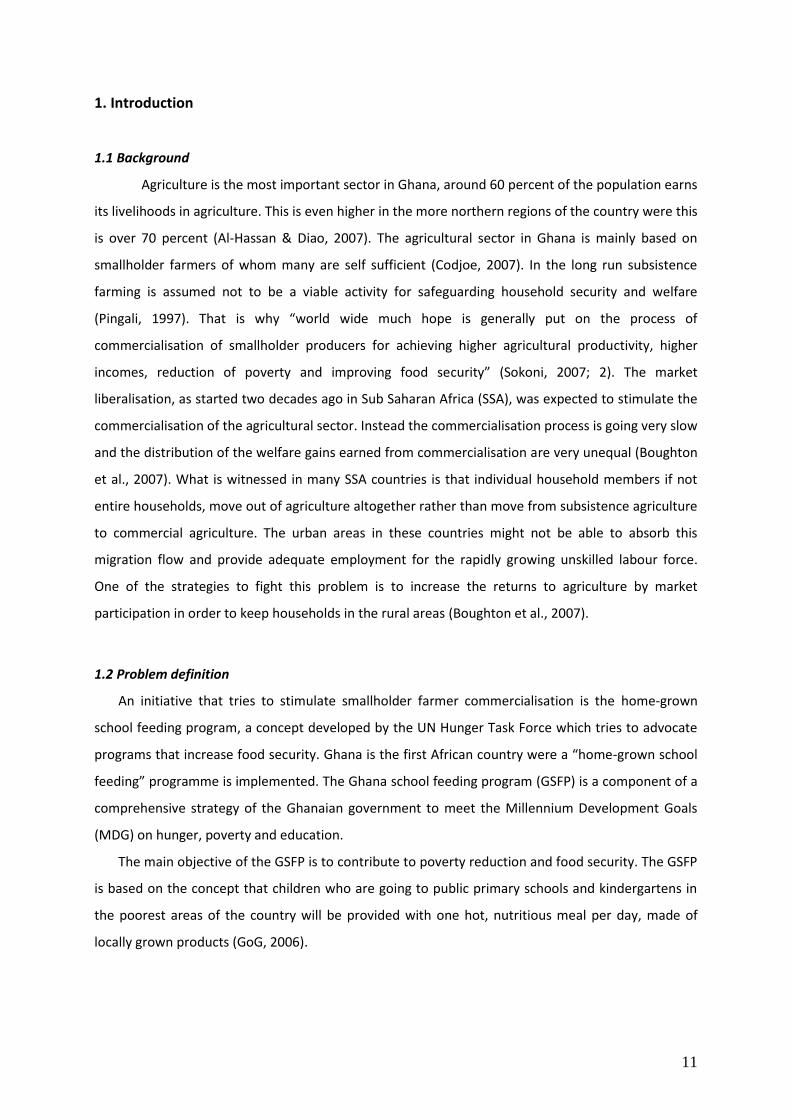
LIST OF FIGURES AND TABLES

LIST OF FIGURES

Page

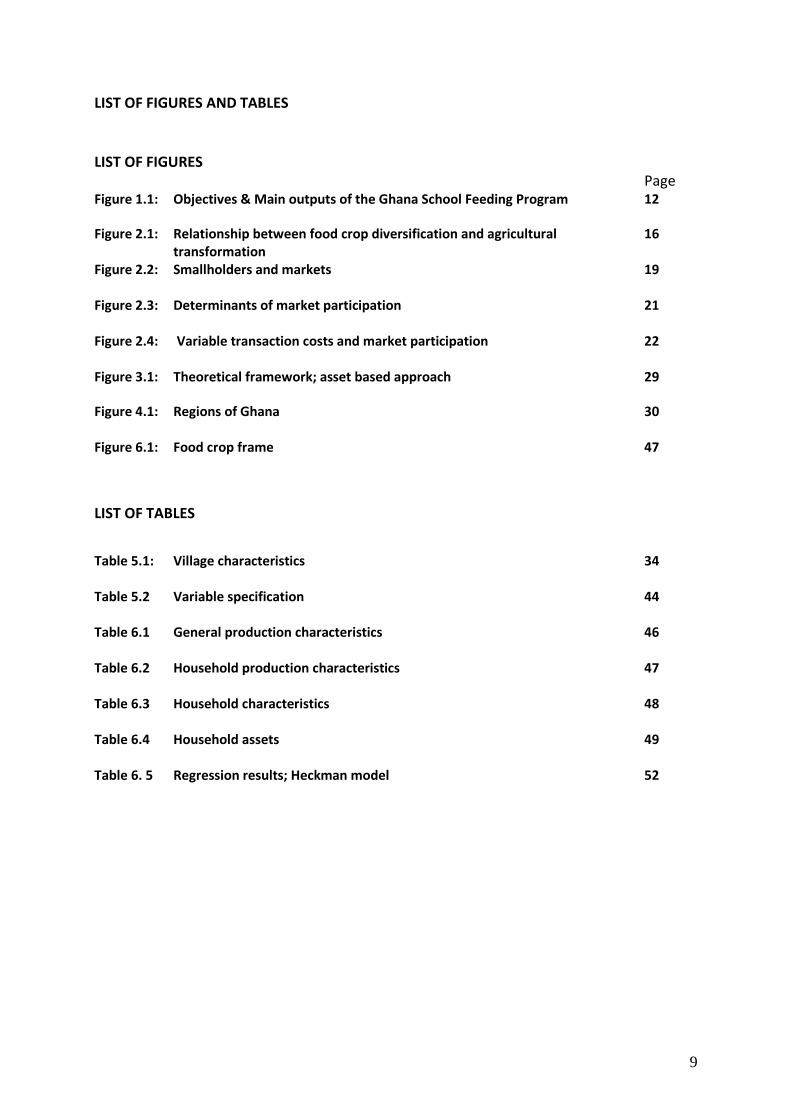
Figure 1.1: Objectives & Main outputs of the Ghana School Feeding Program

12

Figure 2.1: Relationship between food crop diversification and agricultural transformation

16

Figure 2.2: Smallholders and markets

19

Figure 2.3: Determinants of market participation

21

Figure 2.4: Variable transaction costs and market participation

22

Figure 3.1: Theoretical framework; asset based approach

29

Figure 4.1: Regions of Ghana

30

Figure 6.1: Food crop frame

47

LIST OF TABLES

Table 5.1: Village characteristics

34

Table 5.2 Variable specification

44

Table 6.1 General production characteristics

46

Table 6.2 Household production characteristics

47

Table 6.3 Household characteristics

48

Table 6.4 Household assets

49

Table 6. 5 Regression results; Heckman model

52

10

Acknowledgement

In front of you lies my thesis which is part of the fulfilment of the Master International

Development Studies. This thesis would not have been as it is today without the help and support of

many people to whom I want to express my gratitude.

Fist of all, I want to express my gratitude to Mr Eenhoorn for setting up the research project

and giving me the opportunity to be part of it. Moreover, thanks to Gertjan Becx from Resilience for

organising the whole project and supporting my ideas. I thank Xplore for making this research

financially possible. Furthermore, I want to thank Seidhu Al-hassan for his help in the field and the

farmers that participated in this study for their co-operation and hospitality. I would also like to

thank Dr. Nico Heerink for his support and comments on my thesis.

Additionally, I thank Jiska, Esther and Liz for supporting me, listening to my problems and for

making me smile whenever necessary, you’re the best! Jenneke and Chris thanks a lot for the good

time in Ghana and the interesting discussions.

Last but not least I want to thank my parents for their support and encouragement during my

entire study, their patience and faith in me. You were always there when I needed you, thank you for

everything.

11

1. Introduction

1.1 Background

Agriculture is the most important sector in Ghana, around 60 percent of the population earns

its livelihoods in agriculture. This is even higher in the more northern regions of the country were this

is over 70 percent (Al-Hassan & Diao, 2007). The agricultural sector in Ghana is mainly based on

smallholder farmers of whom many are self sufficient (Codjoe, 2007). In the long run subsistence

farming is assumed not to be a viable activity for safeguarding household security and welfare

(Pingali, 1997). That is why “world wide much hope is generally put on the process of

commercialisation of smallholder producers for achieving higher agricultural productivity, higher

incomes, reduction of poverty and improving food security” (Sokoni, 2007; 2). The market

liberalisation, as started two decades ago in Sub Saharan Africa (SSA), was expected to stimulate the

commercialisation of the agricultural sector. Instead the commercialisation process is going very slow

and the distribution of the welfare gains earned from commercialisation are very unequal (Boughton

et al., 2007). What is witnessed in many SSA countries is that individual household members if not

entire households, move out of agriculture altogether rather than move from subsistence agriculture

to commercial agriculture. The urban areas in these countries might not be able to absorb this

migration flow and provide adequate employment for the rapidly growing unskilled labour force.

One of the strategies to fight this problem is to increase the returns to agriculture by market

participation in order to keep households in the rural areas (Boughton et al., 2007).

1.2 Problem definition

An initiative that tries to stimulate smallholder farmer commercialisation is the home-grown

school feeding program, a concept developed by the UN Hunger Task Force which tries to advocate

programs that increase food security. Ghana is the first African country were a “home-grown school

feeding” programme is implemented. The Ghana school feeding program (GSFP) is a component of a

comprehensive strategy of the Ghanaian government to meet the Millennium Development Goals

(MDG) on hunger, poverty and education.

The main objective of the GSFP is to contribute to poverty reduction and food security. The GSFP

is based on the concept that children who are going to public primary schools and kindergartens in

the poorest areas of the country will be provided with one hot, nutritious meal per day, made of

locally grown products (GoG, 2006).

12

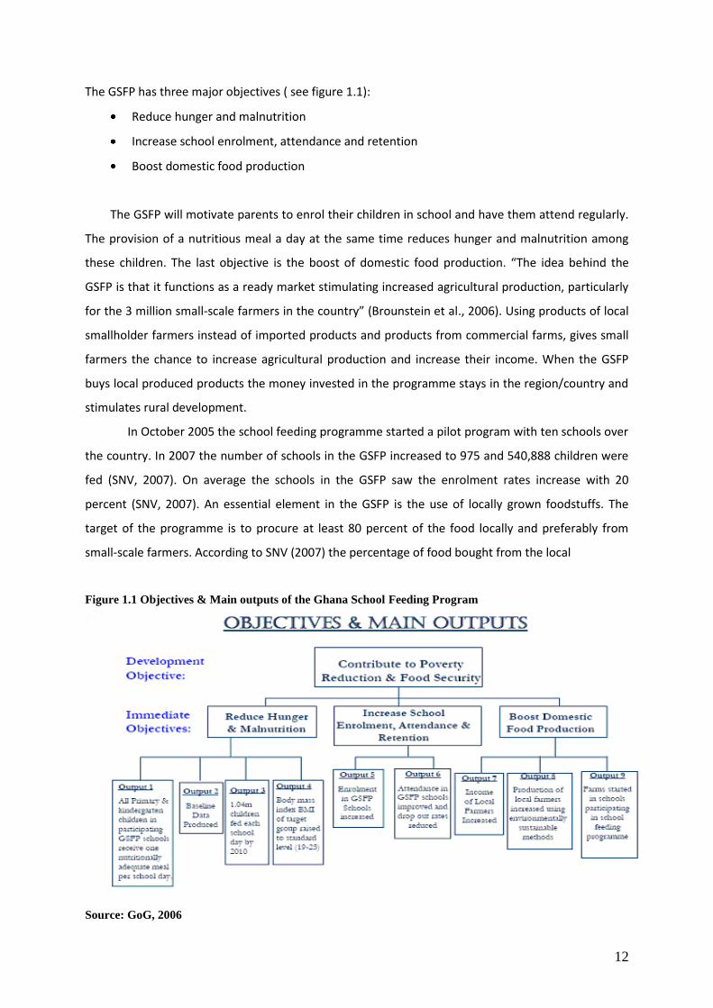
The GSFP has three major objectives ( see figure 1.1):

Reduce hunger and malnutrition

Increase school enrolment, attendance and retention

Boost domestic food production

The GSFP will motivate parents to enrol their children in school and have them attend regularly.

The provision of a nutritious meal a day at the same time reduces hunger and malnutrition among

these children. The last objective is the boost of domestic food production. “The idea behind the

GSFP is that it functions as a ready market stimulating increased agricultural production, particularly

for the 3 million small-scale farmers in the country” (Brounstein et al., 2006). Using products of local

smallholder farmers instead of imported products and products from commercial farms, gives small

farmers the chance to increase agricultural production and increase their income. When the GSFP

buys local produced products the money invested in the programme stays in the region/country and

stimulates rural development.

In October 2005 the school feeding programme started a pilot program with ten schools over

the country. In 2007 the number of schools in the GSFP increased to 975 and 540,888 children were

fed (SNV, 2007). On average the schools in the GSFP saw the enrolment rates increase with 20

percent (SNV, 2007). An essential element in the GSFP is the use of locally grown foodstuffs. The

target of the programme is to procure at least 80 percent of the food locally and preferably from

small-scale farmers. According to SNV (2007) the percentage of food bought from the local

Figure 1.1 Objectives & Main outputs of the Ghana School Feeding Program

Source: GoG, 2006

13

communities or the neighbouring communities is below 20 percent1. Most of the products used for

preparing the school meals are either imported from abroad or produced by large commercial

farmers (Brounstein et al., 2006). This way small-scale farmers hardly benefit from the project. The

project’s target is to raise small-scale farmers income and reduce poverty among them by the use of

a “ready” market, but markets can only stimulate wealth creation among those who can afford to

participate in markets (Boughton et al., 2007). An important factor for the ability of a household to

participate in the market is the asset portfolio which determines the opportunity set (Bruntrup &

Heidhues, 2002).

The problems on the production side of the GSFP made one of the initiators of the GSFP, Mr.

Eenhoorn, decide to research the constraints smallholder farmers face in becoming more market

oriented. Mr Eenhoorn in cooperation with Resilience foundation started the research project:

Transforming poor smallholders into entrepreneurs in sub-Saharan Africa: A pathway for

development. This study is part of this research project.

The team members of the project were divided over the four selected regions: Northern

regions, Upper East, Upper west and Central region. I was placed in the Northern region and

stationed in Tamale. Due to practical reasons, the language barrier of the enumerator assigned to

and transportation limitations, the study focuses one district in the region, Savelugu-Nanton. This

district can be visited on a daily basis from Tamale and the language spoken is known by the

enumerator

1.3 Research objective

The aim of this research is to analyze the asset portfolio of smallholder farmers in order to

determine the constraints imposed by assets holdings on market participation. This will contribute to

the research project of Resilience foundation on Transforming poor smallholders into entrepreneurs

in sub-Saharan Africa: A pathway for development.

1.4 Research questions

Main Question

How does the asset portfolio of smallholder farmers in Ghana influence the participation in food crop

markets?

1 SNV indicates that the 20 percent might not be the correct percentage as the percentages are estimates by

the headmaster and the School Implementation Committee members, but it does give an idea of the situation.

14

Specific questions

Does market access depend on the households’ initial asset endowments?

Which assets are important for crop market entrance?

Which assets influence the degree of participation?

1.5 Justification

The GSFP uses a market-based development strategy. Only those farmers who are able to

produce for the market can profit from the programme. When poorer households are not able to

participate in the market due to their asset endowment, support to build up their private stock of

productive assets and/or the public goods that support production and marketing might be essential.

This explains why it is necessary to correctly identify the asset portfolios that small-scale farmers

need to participate in markets as a first step in the design of programs and policies that stimulate

participation through asset accumulation.

1.6 Contents

This Thesis contains 8 chapters in total. Chapter 2 provides the theoretical background to this

study by discussing the process of commercialisation, the factors determining market participation

and giving an introduction to household models. Further this chapter gives a brief review of the

relevant literature. In chapter 3 the theoretical framework in the form of the asset-based approach is

introduced. The study area in Ghana is described in more detail in chapter 4. The methodology used

for this research is explained in chapter 5 and the results of the data analysis in chapter 6. Chapter 7

looks at the perceived constraints of the small holder farmers and chapter 8 gives the conclusion of

the research and discusses the limitations of the study.

15

2. Theoretical background

This chapter will discuss the commercialisation process of the agricultural sector, which is

supposed to enhance increased market participation. An impression is given of the farmers that are

involved in this process. The chapter continues with a discussion of the factors that influence the

market participation of small-holder farmers and discusses household modelling approaches that can

be used to analyse the market supply behaviour of farm households. The chapter finishes with a brief

overview of empirical studies that examine the impact of asset portfolios on increased market

participation of farm households.

2.1 Commercialisation

Along with economic development starts the structural transformation of the economy. Part

of this process is the transformation of the agricultural sector from diversified subsistence oriented

production towards specialised production for the market.

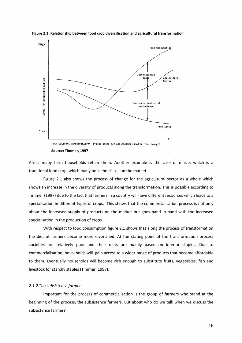
Figure 2.1 shows the relationship between the agricultural transformation and agricultural

diversification showing a stylized representation of the commercialisation process. The process is

divided over three different phases. At the early stage of the agricultural transformation farm

households produce a wide diversity of products mainly for their own consumption. Specialisation of

production is not common. At this point in time farm households have to deal with imperfect

markets for inputs and outputs, risks and uncertainties. Along with economic development the

markets for inputs and output start to develop which creates opportunities for farmers to specialise

in the production of one or a few crops (Timmer, 1997). The subsistence farmers will gradually move

towards being semi-commercial and finally will become commercial producers.

“The commercialization of agricultural systems leads to greater market orientation of farm

production; progressive substitution out of non-traded inputs in favour of purchased inputs, and the

gradual decline of integrated farming systems and their replacement by specialized enterprises for

crop, livestock, poultry and aquaculture products” (Pingali & Rosegrant, 171). The product choice and

input use decisions are more and more based on the principles of profit maximization, shifting

production from staple crops to high value cash crops (Pingali, 1997). Unfortunately this is not a

suitable option for all small-holder farmers. Many small-holder farmers own low-potential and

marginal lands on which the production of traditional crops, often staples, is more suitable (Pingali et

al., 2005). According to Von Braun (1994) the traditional food crops are often marketed as well to a

considerable extent and the cash crops are retained to a substantial extent on the farm for home

consumption. As an example he refers to the situation of groundnut, which is a cash crop but in West

16

Africa many farm households retain them. Another example is the case of maize, which is a

traditional food crop, which many households sell on the market.

Figure 2.1 also shows the process of change for the agricultural sector as a whole which

shows an increase in the diversity of products along the transformation. This is possible according to

Timmer (1997) due to the fact that farmers in a country will have different resources which leads to a

specialisation in different types of crops. This shows that the commercialisation process is not only

about the increased supply of products on the market but goes hand in hand with the increased

specialisation in the production of crops.

With respect to food consumption figure 2,1 shows that along the process of transformation

the diet of farmers become more diversified. At the stating point of the transformation process

societies are relatively poor and their diets are mainly based on inferior staples. Due to

commercialisation, households will gain access to a wider range of products that become affordable

to them. Eventually households will become rich enough to substitute fruits, vegetables, fish and

livestock for starchy staples (Timmer, 1997).

2.1.2 The subsistence farmer

Important for the process of commercialization is the group of farmers who stand at the

beginning of the process, the subsistence farmers. But about who do we talk when we discuss the

subsistence farmer?

Figure 2.1: Relationship between food crop diversification and agricultural transformation

Source: Timmer, 1997

17

A subsistence farmer is a term that is quite vague and it is measured in different ways. The

definition often used in agricultural economics for defining a subsistence farmer focuses on the share

of production devoted to the family’s own consumption. Thus a farmer who “predominantly”

produces for his or her own family’s consumption is labelled a subsistence farmer. If production for

the market dominates, the farmer is considered a commercial farmer. The percentage that a farmer

needs to produce for the market is arbitrary, often the 50 percent line is used (Bruntrup & Heidhues,

2002). In some way farmers are always engaged in some form of trade, by barter, monetized barter

or open markets and are never completely autarkic (Bruntrup & Heidhues, 2002).

Kostov and Lindgren (2004) indicate a distinction between two types of subsistence farmers,

those who are subsistence-oriented and those who are market-oriented. The main motive of a

subsistence-oriented farmer is to protect its own consumption. He will only sell his products in case

of a marketable surplus. The decision to be self-sufficient is made ex-ante of the farming season. The

difference with the market-oriented farmer is based on his ability to plan production for the market.

The quantity marketed is positively correlated to the price and the residual is used for consumption.

Subsistence farming is a method to protect a families livelihood, but it leads to a low

standard of living. Besides that an economy cannot rely on the production of subsistence farmers. It

cannot be expected that these farmers provide a continuous food supply, which is a problem for a

country’s urban population. The irregular pattern of supply leads to high price instability on food

markets which is an undesirable situation. Due to the fact that subsistence farming is a result of risk

averse behaviour, it is difficult to control and direct with policies and programs (Bruntrup &

Heidhues, 2002).

Ellis (1988) argues that when we define farmers by their level of “subsistence” we only look

at a partial aspect of a big group of farmers and leave out many other important aspects which

better defines this group of people. In his work Ellis prefers to talk about peasants. “Peasant are farm

households, with access to their means of livelihood in land, utilizing mainly family labour in farm

production, always located in a larger economic system, but fundamentally characterised by partial

engagement in markets which tend to function with a high degree of imperfection”( Ellis, 1988; 12).

In this definition Ellis focuses on farmers that mainly obtain their livelihood from the land, often by

cultivating crops. Rural dwellers such as landless labourers, plantation workers, pastoralists, or

nomads are excluded from the concept of the peasant farmer.

Important for the distinction between the peasant farmer and the family farmer is the partial

engagement in markets and the incomplete product and factor markets in which they operate. The

peasant farmer unlike the family farmer will have to deal with some or all of the following conditions

18

in his or her daily life (Ellis, 1988):

Fragmented or non-existing capital markets

Variable production inputs are erratically available or unavailable

Poor, erratic, fragmentary and incomplete market information

A freehold market for land does not exist everywhere. And in cases where it exist

open market transactions in land are scarce

Locked factor markets

Ellis’ definition of the peasant farmer allows to focus on a specific group of farmers and is

used to indicate the group of farmers that are studied in this thesis. It makes it possible to look at a

broader segment of farmers than the definition of the subsistence farmer which makes Ellis

definition more suitable to work with.

By focussing on peasant farmers the first and second phase of the agricultural

transformation process will be of main interest. The first phase describes the situation in which the

peasant farmer is still a subsistence-oriented producer as described by Kostov and Lindgren (2004).

A large share of the peasant farmers find themselves in this stage of development where integration

in markets is limited due to the risks and uncertainties of imperfect markets and limited formal

mechanisms to cope with the risks of crop failure (Timmer, 1997). To protect their families’

consumptive needs, production is focussed on feeding their families directly. That is why a wide

variety of crops is produced instead of specialisation in one or a few crops. The ongoing process of

commercialisation will direct the subsistence oriented farmer towards becoming a market oriented

subsistence farmer which is able to plan production for the market. When farmers produce for

markets, specialisation becomes more and more widespread as is shown in figure 2.1. The farmer no

longer has to produce al the crops he wants to consume by himself but can buy them on the market,

which is due to comparative advantages more efficient. The process of specialisation and higher

dependency on factor markets leads farmers eventually to reach the semi-commercial phase in

which they still produce some crops for their own consumption. Essential for this step is the

development of factor markets that reduces the risks of specialisation. Crucial for identifying the

peasant is when in the commercialisation process a farmer is no longer defined as a peasant, but a

family farm enterprise. Ellis (1988) identifies one important element by which such a distinction can

be made namely: “ the degree of specialisation and commitment to market transactions which would

make it infeasible to continue farming in the face of a collapse of market prices of any duration”

(Ellis, 1988; 13). At that point the farmer is no longer able to return to a subsistence-oriented state.

This point of transition is not at a very clear point.

19

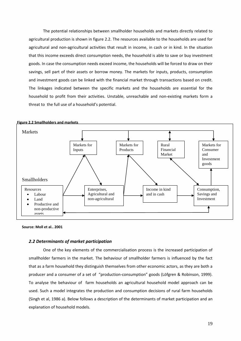
The potential relationships between smallholder households and markets directly related to

agricultural production is shown in figure 2.2. The resources available to the households are used for

agricultural and non-agricultural activities that result in income, in cash or in kind. In the situation

that this income exceeds direct consumption needs, the household is able to save or buy investment

goods. In case the consumption needs exceed income, the households will be forced to draw on their

savings, sell part of their assets or borrow money. The markets for inputs, products, consumption

and investment goods can be linked with the financial market through transactions based on credit.

The linkages indicated between the specific markets and the households are essential for the

household to profit from their activities. Unstable, unreachable and non-existing markets form a

threat to the full use of a household’s potential.

2.2 Determinants of market participation

One of the key elements of the commercialisation process is the increased participation of

smallholder farmers in the market. The behaviour of smallholder farmers is influenced by the fact

that as a farm household they distinguish themselves from other economic actors, as they are both a

producer and a consumer of a set of “production-consumption” goods (Löfgren & Robinson, 1999).

To analyse the behaviour of farm households an agricultural household model approach can be

used. Such a model integrates the production and consumption decisions of rural farm households

(Singh et al, 1986 a). Below follows a description of the determinants of market participation and an

explanation of household models.

Markets

Smallholders

Resources

Labour

Land

Productive and

non-productive

assets

Enterprises,

Agricultural and

non-agricultural

Income in kind

and in cash

Consumption,

Savings and

Investment

Markets for

Inputs

Markets for

Products

Rural

Financial

Market

Markets for

Consumer

and

Investment

goods

Source: Moll et al., 2001

Figure 2.2 Smallholders and markets

20

2.2.1 Determinants of market participation

There is a wide range of factors that influence the decision of farm households to participate

in markets. Figure 2.3 shows the structure of the environment in which a farm household finds itself

and the factors that influence the household’s market participation decision. Bruntrup & Heidhues

(2002) grouped the determining factors of market participation in three categories; country external

factors (outer circle), farm external/country internal factors (intermediate circle) and farm household

internal factors (inner circle).

The factors outside the circle create the boundaries within which a society has to function.

These factors cannot be changed by the society itself and need to be dealt with. The intermediate

circle shows us the institutional and political environment of this society. The inner circle represent

the household resource endowment which determines their opportunity set. This opportunity set

creates the basis for the market participation options a farm household has as it determines its

production options. The market participation decisions made by the farm household depend on the

context in which they are living, which is based on the institutional and political environment. This

environment determines their access to markets and the risk of making market-oriented decisions,

which are crucial factors for the determination of the farm household his resource allocation

(Bruntrup & Heidhues, 2002). The resource allocation in the end determines the direction the

household takes, whether it focuses on producing for the market or that its main goal is to protect its

household consumption level. The two different directions are determined by the situation a farm

household finds itself in.

In the literature on smallholder farmers the determinants of their market participation have

received considerable attention. In this section three different subjects within this field will be

shortly discussed. First of all the impact of transaction costs, followed by risk and risk management

strategies and finally the consequences of a farm household’s asset portfolio.

Transaction costs

Since the early 1990s theorists have tried to model the effects of transaction costs on

agricultural supply and market behaviour for example ; Goetz, 1992 ; Fafchamps, 1992; Key, Sadoulet

and de Janvry, 2000 and de Janvry and Sadoulet, 2006. Transaction costs can be considered as

household external factors, see figure 2.3, due to the fact that these costs are related to the

institutional and political environment in which the household finds itself.

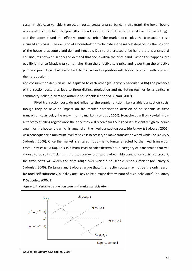
Sadoulet and De Janvry (1995) explain the decision of farm households to participate in the

market by looking at the fixed and variable transaction costs and the price wedge that transaction

costs create between sale and purchase price. Figure 2.4 shows that the existence of transaction

21

22

costs, in this case variable transaction costs, create a price band. In this graph the lower bound

represents the effective sales price (the market price minus the transaction costs incurred in selling)

and the upper bound the effective purchase price (the market price plus the transaction costs

incurred at buying). The decision of a household to participate in the market depends on the position

of the households supply and demand function. Due to the created price band there is a range of

equilibriums between supply and demand that occur within the price band. When this happens, the

equilibrium price (shadow price) is higher than the effective sale price and lower than the effective

purchase price. Households who find themselves in this position will choose to be self-sufficient and

their production.

and consumption decision will be adjusted to each other (de Janvry & Sadoulet, 2006) The presence

of transaction costs thus lead to three distinct production and marketing regimes for a particular

commodity: seller, buyers and autarkic households (Pender & Alemu, 2007).

Fixed transaction costs do not influence the supply function like variable transaction costs,

though they do have an impact on the market participation decision of households as fixed

transaction costs delay the entry into the market (Key et al, 2000). Households will only switch from

autarky to a selling regime once the price they will receive for their good is sufficiently high to induce

a gain for the household which is larger than the fixed transaction costs (de Janvry & Sadoulet, 2006).

As a consequence a minimum level of sales is necessary to make transaction worthwhile (de Janvry &

Sadoulet, 2006). Once the market is entered, supply is no longer affected by the fixed transaction

costs ( Key et al, 2000). This minimum level of sales determines a category of households that will

choose to be self-sufficient. In the situation where fixed and variable transaction costs are present,

the fixed costs will widen the price range over which a household is self-sufficient (de Janvry &

Sadoulet, 2006). De Janvry and Sadoulet argue that: “transaction costs may not be the only reason

for food self sufficiency, but they are likely to be a major determinant of such behaviour” (de Janvry

& Sadoulet, 2006; 4).

Figure: 2.4 Variable transaction costs and market participation

Source: de Janvry & Sadoulet, 2006

23

Risk and anti-risk management

Another explanation for the lack of market participation of smallholder farmers discussed in

the literature is the risk averse behaviour of the farm household. High income risk is part of life for

farm households in developing countries. Risk-based explanations try to analyse the household

behaviour with respect to a wide variety of risks. Farm households are exposed to risks which are

the result of their ecological, infra-structural and institutional environment, represented in figure 2.3

by the outer and intermediate circle (Bruntrup & Heidhues, 2002). The impact of an unfavourable

event, such as drought, pests or market failure, on poor small holder farmers are far reaching, it can

lead to income loss, lack of food provision, lack of basic social security which in turn can cause

hunger and starvation, and so stimulates risk averse behaviour. For many smallholder farmers

“subsistence agriculture is a protection of households against extreme and unpredictable risks”

(Bruntrup & Heidhues, 2002; 14).

De Janvry and Sadoulet (2006) only used the concept of risk with respect to prices. They

discuss the impact of price risks on the production decision of farm households. The volatility of

prices leads to a situation in which farmers are uncertain whether the price they will receive at the

market will cover the costs they make during the farm season. The price risks combined with the

degree of risk aversion of the household influences the effective price that is used for decision

making (Sadoulet & de Janvry, 1995). Sales prices are discounted in a negative way and purchase

prices in a positive manner which widens the price band as discussed under transaction costs. The

widening of the price band increases the range in which households prefer to stay autarkic negatively

influencing the market participation of these households.

Asset portfolio

A relatively less researched strand of literature tries to relate market participation of small

holder farmers in (specific) crop markets to their asset portfolio as a whole instead of one single

aspect of this portfolio. The asset portfolio is considered in a broad sense and goes beyond the

traditional productive tangible assets; natural, human, physical and financial capital. It often includes

intangible assets as well which can be classified as social assets and locational assets, this is

represented by the inner circle of figure 2.3 which describes the opportunity set of a farm household.

The household’s supply of food crops depends on the opportunity set which is based on the

households asset portfolio.

With this type of research scholars try to identify which assets strongly relate to the market

participation of smallholder farmers and if the participation in higher return markets require

different asset portfolios. If asset poor farm households have problems participating in commercial

24

markets then stimulating increased smallholder agricultural commercialization may fail when

you do not focus on building up the right assets (Boughton et al, 2007).

2.2.2 Household model approaches

The analysis of farm household behaviour has taken different directions over time. Timmer

(1997) identifies two extreme point of views with regard to farm household behaviour. First of all

there is the point of view that subsistence farmers do not participate in any market activity or want

to use new production technology due to the fear of losing their income. To understand the

behaviour of such farm households one needs to understand their cultural traditions, technical

constraints and the variability of their environment. The substantivist school in economic

anthropology even rejected the use of formal economic analysis based on optimization behaviour.

According to them peasants do not maximize their utility but are just motivated by the satisfaction of

their needs (de Janvry et al, 1991). They see the behaviour of the farm household as non-economic

behaviour.

Opposite to this point of view stands the idea that is based on the neoclassical assumptions

of perfect and complete markets, absence of transaction costs and full information available to all

participants (Timmer, 1997). Decision making in such an environment is solely based on the

parametric prices for factors and commodities in rural markets. As long as the marginal costs equal

marginal revenues there exists a situation in which both maximum social and individual welfare are

guaranteed.

The farm household distinguishes itself by the fact that it is both a producer and a consumer

of a set of “production-consumption” goods; i.e. goods that are both supplied and demanded by the

household, for example, food products and family time (used as labour or leisure) (Löfgren &

Robinson, 1999). Due to the integration of consumption, production and labour decisions in farm

households it is not possible to analyse these decisions separately by looking at the behaviour of

three classes of agents; producers, consumers and workers (Sadoulet & de Janvry, 1995). To analyse

farm household behaviour a household model would be a better instrument, as the decision on

production, consumption and work are then integrated into one single household problem.

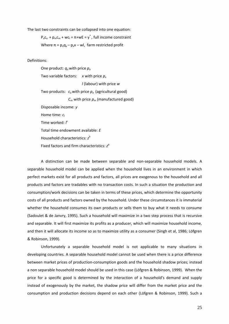
Structural form of the model2:

Max u(ca , cm , cl ; zh), utility function

s.t.: g(qa , x,l;zq ) = 0, production function,

pxx + pm cm = pa (qa – ca ) + w(ls – l), cash constraint,

cl + ls =E, time constraint.

2 Based on Sadoulet & de Janvry, 1995

25

The last two constraints can be collapsed into one equation:

Paca + pmcm + wcl = π+wE = y* , full income constraint

Where π = paqa – pxx – wl, farm restricted profit

Definitions:

One product: qa with price pa

Two variable factors: x with price px

l (labour) with price w

Two products: ca with price pa (agricultural good)

Cm with price pm (manufactured good)

Disposable income: y

Home time: cl

Time worked: ls

Total time endowment available: E

Household characteristics: zh

Fixed factors and firm characteristics: zq

A distinction can be made between separable and non-separable household models. A

separable household model can be applied when the household lives in an environment in which

perfect markets exist for all products and factors, all prices are exogenous to the household and all

products and factors are tradables with no transaction costs. In such a situation the production and

consumption/work decisions can be taken in terms of these prices, which determine the opportunity

costs of all products and factors owned by the household. Under these circumstances it is immaterial

whether the household consumes its own products or sells them to buy what it needs to consume

(Sadoulet & de Janvry, 1995). Such a household will maximize in a two step process that is recursive

and separable. It will first maximize its profits as a producer, which will maximize household income,

and then it will allocate its income so as to maximize utility as a consumer (Singh et al, 1986; Löfgren

& Robinson, 1999).

Unfortunately a separable household model is not applicable to many situations in

developing countries. A separable household model cannot be used when there is a price difference

between market prices of production-consumption goods and the household shadow prices; instead

a non separable household model should be used in this case (Löfgren & Robinson, 1999). When the

price for a specific good is determined by the interaction of a household’s demand and supply

instead of exogenously by the market, the shadow price will differ from the market price and the

consumption and production decisions depend on each other (Löfgren & Robinson, 1999). Such a

26

situation occurs in the case of market imperfection and failures (de Janvry & Sadoulet, 2006). Farm

households in developing countries are systematically exposed to imperfect markets and to analyse

their behaviour a non-separable household model should be used.

The difference between the models thus lies in the linkages between consumption and

production decisions. In a separable model production and consumption decisions are only linked

through the level of farm income achieved in production. This in contrast with the non-separable

model where there are direct interrelations between production and consumption decisions.

2.3 Empirical studies

Literature focussing specific on the impact of asset endowment on farm household

participation in crop markets is not very extensive. Studies done so far do find links between the

assets held by a household and their market participation. The three studies discussed here did

research on data from Mozambique.

In their article Heltberg and Tarp (2002) make a distinction between the decision to participate and

the decision of how much to sell based on household data from the 1996-7 Inquérito Nacional aos

Agregados Familiares sobre as Condições de Vida (IAF), a general purpose living standard survey.

They distinguish in their analysis between food crops, cash crops and the total sales. The assets that

they found having a significant effect for market participation differed between food crops, cash

crops and total sales. They conclude that farmers who are relatively well endowed with agricultural

capital and land are the ones most likely to commercialise. The farm size, log number of trees and

the ownership of traction equipment were all positively associated with the decision to participate in

the market and the degree of participation in relation to total output sales. For food crops the farm

size and the log number of trees were positively related to the decision to participate in the market.

For cash crops, the farm size positively affected the decision to participate. Heltbeg and Tarp (2002)

also discuss the impact of transaction costs on market participation. They make a distinction

between variable transaction costs and fixed transaction costs. Their most important findings are

that for variable transaction costs transport ownership is positively related to the value of sales and

market participation for total output and for cash crop market participation and for fixed transaction

costs the ownership of communication equipment is significantly and positively related to food crop

market participation. Bougthon et al. (2007) in turn look at the relationship between different asset

portfolios and the participation in different types of crop markets. For their analysis they used

household data from the national agricultural sample survey of 2001-2. They look at differences

between a spot market (maize), contract production for a relatively undifferentiated commodity

(cotton) and contract production of a quality differentiated product (tobacco). They found evidence

of asset-related barriers to entry for each of the studied markets. Their main findings are that the

27

households private assets, especially land, livestock, labour and equipment, positively affect crop

market participation. They also found that the provision of public goods such as infrastructure and

market information does not seem to have a significant effect on crop market participation. A

different approach is used in the work of Benfica et al. ( 2006) in which one specific cash crop,

tobacco, is considered for a specific region in Mozambique, the Zambezi Valley. They conducted a

survey consisting of 159 farmers of whom 117 grew tobacco. They found that the participation in

contract farming schemes was statistically significantly linked to a household’s asset endowment and

alternative income opportunities. The asset that came out as important are; the availability of draft

power, the value of hand tools and the value of production and marketing equipment such as

bicycles. These assets were positively associated with market participation. The alternative income

opportunities that were found significant were income from livestock and wages.

28

3. Theoretical framework

Two approaches that focus on assets and capabilities, institutions and livelihoods are the

Sustainable Livelihood Approach and the Asset Building framework. The last is an umbrella title for a

number of conceptual approaches and frameworks. What distinguishes the two approaches from

each other is the emphasis. “Asset Building frameworks are more specifically concerned with assets,

and associated asset accumulation strategies, rather than more generally with livelihoods as is the

case with the Sustainable Livelihoods Approach” (Moser, 2005; 16). As the focus of this research is

more specific on asset endowments the Asset Building framework will be used as a theoretical frame.

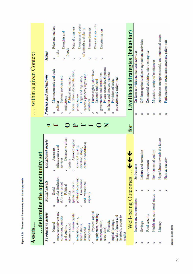
Siegel (2005) introduces a conceptual framework for an asset-based approach in which

household assets are considered the “drivers” of sustainable growth and poverty reduction. Figure

3.1 shows the conceptual framework from Siegel. The asset-based approach is useful to understand

the type and combination of assets that are required by households to take advantage of economic

opportunities and improve their well-being over time (Siegel, 2005).

The framework builds on four blocks that interact with each other: Assets, context,

behaviour and outcomes. The assets of a household determine the opportunity set of options for

livelihood strategies (household revealed behaviour). The chosen strategies in turn lead to outcomes

in terms of household well-being. This whole process is influenced by the context in which the

situation takes place.

The assets in the asset-based approach not only include the traditional productive tangible

assets as natural, human, physical and financial capital but incorporate intangible assets as well

(Siegel & Alwang, 1999). The intangible assets are divided in social assets and locational assets (see

figure 3.1). “The quantity and quality of assets, and their complementary determine households well-

being and growth potential, for a given context” (Siegel, 2005; 9). The context households face exists

of the political and institutional environment, defining ownership and acceptable use of assets and

risk factors. To be able to deal with risk, households use risk management strategies. These are

mechanisms that are used to deal with anticipated or actual losses associated with uncertain events

and outcomes (Siegel & Alwang, 1999). Households can use risk reducing, coping and mitigating

strategies to protect themselves. The strategy chosen is influenced by and will influence the asset

portfolio (Siegel & Alwang, 1999).

On basis of the asset portfolio the household is engaged in income generating activities.

These in turn lead to a certain well-being of the household.

29

30

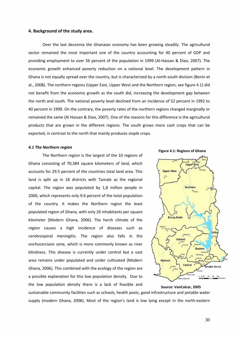
Figure 4.1: Regions of Ghana

4. Background of the study area.

Over the last decennia the Ghanaian economy has been growing steadily. The agricultural

sector remained the most important one of the country accounting for 40 percent of GDP and

providing employment to over 56 percent of the population in 1999 (Al-Hassan & Diao, 2007). The

economic growth enhanced poverty reduction on a national level. The development pattern in

Ghana is not equally spread over the country, but is characterized by a north-south division (Benin et

al., 2008). The northern regions (Upper East, Upper West and the Northern region, see figure 4.1) did

not benefit from the economic growth as the south did, increasing the development gap between

the north and south. The national poverty level declined from an incidence of 52 percent in 1992 to

40 percent in 1999. On the contrary, the poverty rates of the northern regions changed marginally or

remained the same (Al Hassan & Diao, 2007). One of the reasons for this difference is the agricultural

products that are grown in the different regions. The south grows more cash crops that can be

exported, in contrast to the north that mainly produces staple crops.

4.1 The Northern region

The Northern region is the largest of the 10 regions of

Ghana consisting of 70,384 square kilometers of land, which

accounts for 29.5 percent of the countries total land area. This

land is split up in 18 districts with Tamale as the regional

capital. The region was populated by 1,8 million people in

2000, which represents only 9.6 percent of the total population

of the country. It makes the Northern region the least

populated region of Ghana, with only 26 inhabitants per square

kilometer (Modern Ghana, 2006). The harsh climate of the

region causes a high incidence of diseases such as

cerebrospinal meningitis. The region also falls in the

onchocerciasis zone, which is more commonly known as river

blindness. This disease is currently under control but a vast

area remains under populated and under cultivated (Modern

Ghana, 2006). This combined with the ecology of the region are

a possible explanation for this low population density. Due to

the low population density there is a lack of feasible and

sustainable community facilities such as schools, health posts, good infrastructure and potable water

supply (modern Ghana, 2006). Most of the region’s land is low lying except in the north-eastern

Source: VanCalcar, 2005

31

corner where we find the Gambaga escarpment and along the western corridor. The region is

drained by the Black and white Volta (Modern Ghana, 2006).

4.1.1 Climate

The Northern region lies in the agro-ecological Guinea savannah zone, which is characterized

by low and erratic rainfall. The amount of rain on an annual basis varies between 750mm and 1050

mm per year (modern Ghana, 2006). The main vegetation is classified as vast areas of grassland,

interspersed with the guinea savannah woodland, characterised by drought-resistant trees such as

the acacia, baobab, shea nut, dawadawa, mango and neem (Modern Ghana, 2006). The area has a

long dry season that ranges from November to April. In this period the region also has to deal with

exceptionally strong and dry winds, the harmattan. There is only one rainy season which starts in late

April or early May. “About 90 % of the rainfall is received between June and September and only

within these humid months do soil moisture surplus occur” (ISSER, 200X; 5). This is the time that

enables the farmers to grow their crops. In the dry season farmers are only able to cultivate land

under irrigation. As irrigation is not widespread in the area, most farmers are idle during the dry

season. Rain fed farming is the common practice in the area.

4.1.2 Ethnicity

The region is populated by a diverse range of ethnic groups. The four main groups, all

represented by their own paramount chief, are the Mole Dagbon (52.2 %), the Gurma (21.8 %), The

Akan and the Guan (8.7 %). The largest subgroup are the Dagomba belonging to the Mole Dagbon

ethnic group. They constitute around one third of the population in the region.

The main religion in the region is Islam, which around 56.2 percent follow. The rest of the

population can be broadly divided between Animists (21.3 %) and Christians (19.3%)(Modern Ghana,

2006).

4.2 Savelugu-Nanton district

Savelugu-Nanton is one of the 18 districts of the Northern region (see Annex I for the map of

the Northern region). It lies above Tamale municipality and is well connected to this district by the

Tamale- Bolgatanga road. Savelugu-Nanton is one of the smaller districts of the Northern region

with a land area of 1,790 square kilometers. The district has a higher population density with 61

persons per square kilometer than the region itself but it is still lower than the national average of

78.9. The southern part of the district is more densely populated than the north. Of the 149

communities that are found in the district, 143 are defined as rural. Around 80 percent of the

32

population resides in these rural settlements. The district is governed from Savelugu, the most

important urban centre of the district (Ghana districts, 2008).

4.2.1 Agriculture

The agricultural sector is very important in this district as 97 percent of the labor force is

engaged in farming (Unicef, 1999; Ghana districts, 2008). The majority of these people is engaged in

the production of staple crops at the subsistence level. For 63.2 percent of the people this is their

only source of income (Unicef, 1999). The district is located in the interior savanna woodland, where

it receives an annual rainfall averaging 600mm. The area is most suitable for livestock and staple crop

production. The most important crops that are grown in the area are maize, guinea corn, millet, rice,

yam, groundnut, cowpea and soybean. Maize is the most important crop for the people of Savelugu-

Nanton, it is the main ingredient for T.Z. the dish that is served almost daily. Additional to the annual

crops, tree crops play an important role as well, especially shea trees for shea butter and the Dawa

Dawa for condiments. These products often serve as a source of additional income especially for

women. Dry season farming is rare in Savelugu-Nanton with only a few irrigation projects, but new

projects are planned to be developed (Ghana districts, 2008).

4.2.2 Infrastructure

Most of the communities are interconnected by feeder roads, but over 50 percent of these

dirt roads are impassable by motor vehicles seasonally. There is one well functioning asphalt road

which is the Tamale-Bolgatanga road. Transport possibilities to 80 percent of the rural communities

that are not lying near this road is poor, especially in the rainy season, making the transport of food

crops difficult. Bicycles are therefore a very important way of transport.

Access to electricity is not common in Savelugu-Nanton. Around 11 percent of the

communities was connected to the system in 2006.

Access to potable water sources is limited in this district. Less than 50 percent of the

population has access to safe water: treated water, boreholes and hand dug wells. Access to

boreholes is restricted to 34 percent of the population; one third of the boreholes are found in the

area council of Nanton. The majority of the people have to rely on unsafe sources such as dugouts,

dams , ponds, river streams and unprotected wells (Ghana districts, 2008).

4.2.3 Market

The district has four main markets which have a six day schedule. The markets are spread

over the district and are found in Savelugu, Nanton, Tampion and Diare. Besides these large markets

there are markets in smaller communities as well. The markets from neighboring districts in

33

Kumbungu, Tolon, Karaga and Tamale are frequently visited as well. Market days are special in this

region, not only do people go there to buy and sell their products, it is a social meeting place as well

and many, especially the youngsters, attend the market every 6 days.

4.2.4 The Ghana School Feeding Program

In Savelugu-Nanton two schools are beneficiaries of the GSFP. Those are located in Nyologu

and Kpalan/Koduzeigu. In both schools the program was implemented in 2006. Due to financial

issues the schools receive products from the GSFP to prepare two meals per week. For the other

three days the schools receive maize flower from the World Food Program. Each school has an

outside kitchen where four cooks prepare the meals. In Nyology all four are women from the

community. In Kpalan/Koduzeigu there is one male cook and three women, who assist him, from the

community. The main products that the schools receive are rice, beans, gari and maize. This is

supplemented with onion, tomato, red pepper, magi, oil and small fish. Once a month the

headmasters of the schools receive extra money to buy meat. This money is sufficient for one meal.

According to the headmasters this money should come weekly (Personal interviews, 2008).

The District Assembley of Savelugu-Nanton has appointed two female traders to take care of

the food supply to the schools. The school in Nyologu is supplied by Mrs. Ramatu. She buys the

products for the school from the market in Savelugu. According to her this is the only option due to

the limited availability of products in the communities during the lean season. According to her a

group is being set-up in the community to produce oil in the community for the school. No

arrangements with farmers have been made for food crop supply.

34

5. Methodology

This chapter will focus on the methodology used for the analysis. The first section will discus

the collection process of the data and the sampling method chosen for the data collection. In the

second section the analytical framework on which the analysis is based will be discussed. This is

followed by the third section that discusses the method of analysis and this chapter will finish with an

overview of the variables used in the analysis.

5.1 Data collection and sampling

For this research a household survey was designed which contained both structured and

semi structured questions. This was done to have qualitative information next to the outcomes from

the statistical analysis based on the structured questions. The survey looked into the food crop

production of small holder farmers and their market participation in food crop markets. To link their

market participation to their asset portfolio, questions were asked concerning their asset

endowment. The semi structured questions focused on the perceived problems of small-holder

farmers to increase their production and participate in food crop markets.

This study focuses on farm households in Savelugu-Nanton which are engaged in food crop

production, which is the main income generating activity in this region. The focus lies on food crops

as they are of importance for the GSFP. In total 90 farm households were interviewed in the 11

strategically selected villages. Two of the villages selected have schools that are part of the GSFP, the

other 9 were selected based on their location in the district. The villages are selected in such a way

that the whole district is geographically covered. Table 5.1 shows the characteristics of the villages

that were used in this research. A map of Savelugu-Nanton district showing the exact location of

each of the villages and so the coverage of the district, can be found in Annex II.

Table 5.1: village characteristics

Village Nr of inhabitants

Sample size

Distance to Tamale (km)

Distance to savelugu market (km)

Distance to nearest market (km)

Access to borehole

Part of the GSFP

Zinindo 3225 15 49 38 14 No No Dipali 686 9 55 34 18 Yes No Sahakpaligu 619 12 15 16 15 No No Zeitigu/Nyamandu 515 10 27 22 10 Yes No Libga 446 10 24 3 3 Yes No Kpalan 372 9 34 13 13 No Yes Nyologu 1137 10 44 36 11 Yes Yes Kpalung 839 5 32 11 11 No No Saakpuli 164 3 80 59 27 yes No Dikping 261 2 70 49 21 Yes No Zosali n.a 5 58 37 9 Yes No

35

The data for the survey were collected from half April to half June 2008. This period

corresponds with the end of the dry season and the beginning of the rainy season. This is the period

in which most of the farmers start with their farm activities causing some difficulties with finding the

head of the farm household, as they were frequently on their farms. It was necessary to speak with

the head of the household as we wanted to discuss financial matters of which he or she is often in

control. At the start of the season there is also a group of farmers who for various reasons decided

to postpone farming activities until later. Some of them preferred to wait for more and heavier rains

and others could not start yet due to financial matters. To get a sample which contained both groups

of farmers the interviews, when possible, took place during the afternoon when most farmers

returned to rest and look for shelter from the sun. The further we moved into the farming season,

the more complicated it became to find farmers who were in the village and were willing to

cooperate. Performing this research in this period might have caused a bias in the sample towards

more risk averse and poorer farmers as they were the ones that were over represented in the village.

This situation as well influenced the number of farmers interviewed per village. The set up was to get

equal samples sizes per village. This appeared not to be manageable considering the timeframe and

the wish to cover the whole district. That is why the decision has been made to accept different

sample sizes per village.

The farm households were selected ad random. The selection of farm households was done

by asking every fourth household in small villages or every tenth household in larger communities on

the path from the center to participate in research. The constraint of this method is that it is possible

that part of the village is left out of the research.

All the interviews were conducted with an enumerator who translated Dagbani to English.

There have been some difficulties with getting answers on the questions concerning livestock

numbers and most specifically the number of cows owned by the household. The questions

concerning credit caused some problems and were answered only in the form of direct cash flows

and not with respect to the provision of inputs or services.

The data collected cover the farm year 2007. This year is characterized by extreme drought at

the start of the farming season which caused problems with the germination of the seeds. Farmers

who had the financial capacity re-sow some of their fields. Later in the season the rains were very

heavy which caused floods. Farmers with low lying fields lost a large share of their production. This

influences the production levels and possibly the market participation behavior of the farm

households.

36

5.2 Analytical framework

In order to analyse a farmer’s market participation a simple model of household choice is

adapted from Boughton et al (2006) and Barrett (2008). This household model focuses on the impact

of asset endowment on market participation.

5.2.1 Theoretical model

The household choice model is based on the assumption that the household maximizes its

utility, defined over consumption of a vector of agricultural commodities, yc for c=1,…..,C and a

Hicksian composition of other tradables, x. The household earns income from production, and

possibly sale, of any or all the crops, C and from off-farm earnings, W. Each crop is produced using a

crop-specific production technology, ƒc(Ac,G), which maps the flow of services provided by privately

held quasi-fixed assets (represented in vector A) and public goods and services (represented by the

vector G).

The choice of the farmer to participate in the crop market as a seller is indicated by the

dependent variable Mcs. This variable can take the value 1 if the household enters the market to sell

a crop and 0 if not. Similarly the household chooses whether or not to buy a crop, represented by

the dependent variable Mcb, taking the value 1 for every crop a household decides to buy. This results

in the net sales of crop NSc ≡ ƒc(Ac,G) – yc.

The choice to participate in the market will be influenced by the net returns to market

participation. Each household faces a parametric market price for each crop, p, and household

specific transaction costs, τc (Z,A,G,W, NSc), where the vector Z stands for household characteristics.

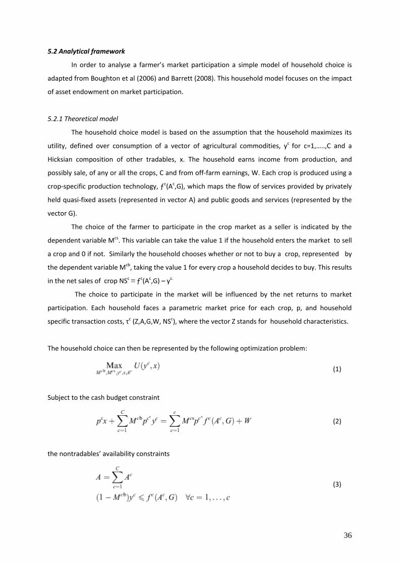
The household choice can then be represented by the following optimization problem:

(1)

Subject to the cash budget constraint

(2)

the nontradables’ availability constraints

(3)

37

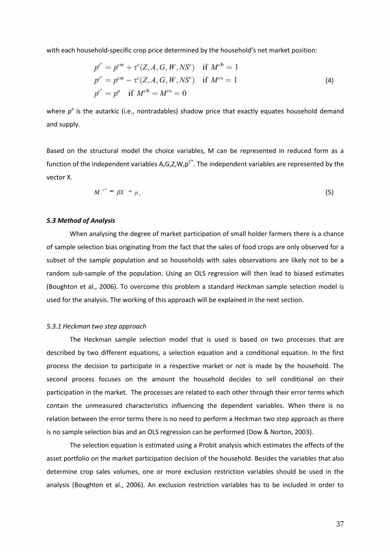
with each household-specific crop price determined by the household’s net market position:

(4)

where pa is the autarkic (i.e., nontradables) shadow price that exactly equates household demand

and supply.

Based on the structural model the choice variables, M can be represented in reduced form as a

function of the independent variables A,G,Z,W,pC*. The independent variables are represented by the

vector X.

i

cμβXM

*

(5)

5.3 Method of Analysis

When analysing the degree of market participation of small holder farmers there is a chance

of sample selection bias originating from the fact that the sales of food crops are only observed for a

subset of the sample population and so households with sales observations are likely not to be a

random sub-sample of the population. Using an OLS regression will then lead to biased estimates

(Boughton et al., 2006). To overcome this problem a standard Heckman sample selection model is

used for the analysis. The working of this approach will be explained in the next section.

5.3.1 Heckman two step approach

The Heckman sample selection model that is used is based on two processes that are

described by two different equations, a selection equation and a conditional equation. In the first

process the decision to participate in a respective market or not is made by the household. The

second process focuses on the amount the household decides to sell conditional on their

participation in the market. The processes are related to each other through their error terms which

contain the unmeasured characteristics influencing the dependent variables. When there is no

relation between the error terms there is no need to perform a Heckman two step approach as there

is no sample selection bias and an OLS regression can be performed (Dow & Norton, 2003).

The selection equation is estimated using a Probit analysis which estimates the effects of the

asset portfolio on the market participation decision of the household. Besides the variables that also

determine crop sales volumes, one or more exclusion restriction variables should be used in the

analysis (Boughton et al., 2006). An exclusion restriction variables has to be included in order to

38

correctly identify the model and prevent multicollinearity and instable parameters in the OLS (Smits,

2003).

The residuals of the selection equation are used to construct a selection bias control factor

called Heckman’s Lambda which equals the Inverse Mill’s Ratio. This factor reflects the effects of all

unmeasured characteristics on the market participation decision (Smits, 2003).

In the second step an OLS regression is performed to analyse the effects of the asset

portfolio on the quantity supplied on the market. Heckman’s Lambda is added as an additional

variable to the equation. By adding a control factor in the form of Heckman’s Lambda, the effect of

the quantity of sales-related unmeasured characteristics, which are also related to the market

participation decision, frees the other predictors in the equation from this effect and the regression

analysis gives unbiased coefficients (Smits, 2003).

5.3.2 Model specification

The Heckman sample selection model has the form (Vella, 1998):

, if P P, M

if P P , MM

μβ X P

μ β XM

ii i

iiii

i

'

ii

i

'

ii

0 0 observednot

0 1

*

**

222

*

111

*

where Mi* is a latent variable with observed counterpart Mi measuring the quantity of sales, Pi* is a

latent variable with associated indicator function Pi reflecting whether the primary dependent

variable is observed i.e. whether a household is participating in the market or not. This resembles the

choice between autarchy and selling regime. A buying regime is not taken into account in this study

due to the problem that households buy small amounts of food crops and could not recall exact

quantities. The relation between Pi and Pi*and Mi and Mi* respectively are shown in (7) and (8),

which is the observation rule. (5) is the equation of primary interest referred to as the conditional

equation and (6) is the selection equation, which is of the binary choice type; X1i and X2i are vectors

of exogenous variables; β1 and β2 are vectors of unknown parameters. The error terms μ1 and μ2 are

zero mean error terms with E *μ1│ μ2+ ≠ 0 . N denotes the entire sample size and n denotes the sub-

sample for which Mi = 1. In this analysis the vector X2 contains at least one variable which does not

appear in X1. These variables are referred to as the exclusion restriction variables (Vella, 1998). In this

research the selection of the exclusion restriction variables are based on previous work from Benfica

(2006) and Boughton (2006). They select variables that measure the household’s dependence on

food crop income. In this research the exclusion restriction variables are the household’s

(5)

(6)

(7)

(8)

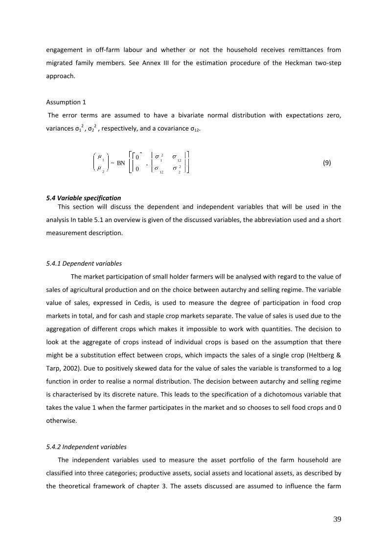
39

engagement in off-farm labour and whether or not the household receives remittances from

migrated family members. See Annex III for the estimation procedure of the Heckman two-step

approach.

Assumption 1

The error terms are assumed to have a bivariate normal distribution with expectations zero,

variances ς12 , ς2

2 , respectively, and a covariance ς12.

2

212

12

2

1

2

1 ,

0

0 BN ~ (9)

5.4 Variable specification This section will discuss the dependent and independent variables that will be used in the

analysis In table 5.1 an overview is given of the discussed variables, the abbreviation used and a short

measurement description.

5.4.1 Dependent variables

The market participation of small holder farmers will be analysed with regard to the value of

sales of agricultural production and on the choice between autarchy and selling regime. The variable

value of sales, expressed in Cedis, is used to measure the degree of participation in food crop

markets in total, and for cash and staple crop markets separate. The value of sales is used due to the

aggregation of different crops which makes it impossible to work with quantities. The decision to

look at the aggregate of crops instead of individual crops is based on the assumption that there

might be a substitution effect between crops, which impacts the sales of a single crop (Heltberg &

Tarp, 2002). Due to positively skewed data for the value of sales the variable is transformed to a log

function in order to realise a normal distribution. The decision between autarchy and selling regime

is characterised by its discrete nature. This leads to the specification of a dichotomous variable that

takes the value 1 when the farmer participates in the market and so chooses to sell food crops and 0

otherwise.

5.4.2 Independent variables

The independent variables used to measure the asset portfolio of the farm household are

classified into three categories; productive assets, social assets and locational assets, as described by

the theoretical framework of chapter 3. The assets discussed are assumed to influence the farm

40

household’s market participation. These variables are complemented with a set of variables

measuring household characteristics and household dependency on food crop income.

Natural capital

Farm size: The number of acres that a family owns. This includes the number of acres of bush and

compound farm and the number of acres that are currently not used for farming. This variable is

assumed to positively influence the participation in food crop markets as it is expected that

ownership of more land will give the opportunity to farm more acres resulting in a larger output that

can be sold.

Human capital

Literacy: This variable measures the household head’s ability to read and write. A literate person is

assumed to have captured a larger amount of knowledge and posses a bigger capacity to gather

information and is therefore expected to run a farm that is better capable of gearing the activities to

the market situation. That is why it is assumed that literacy has a positive impact on the household’s

participation in food crop markets.

Dependency ratio: This variable considers the ratio of non-working to working household members.

This ratio is assumed to negatively influence the participation in food crop markets as the relative

number of household members that can effectively contribute to the household’s income reduces

with an increasing dependency ratio and the number of members that they have to feed increases.

Due to positively skewed data for the dependency ratio this variable is transformed to a log function

in order to realise a normal distribution.

Physical capital

Transport: Ownership of transport equipment in the form of a bicycle or motorbike is assumed to

have a positive effect on market participation. Ownership of such an asset eases transportation of

produce from the field to the house and from the house to the market. This influences the

transaction costs incurred. The farmer has the option to transport the products himself and does not

have to ay for services from others. A reduction in transaction cost influences the price band as

discussed by de Janvry and Sadoulet (1995) which reduces the autarkic state of the household (see

chapter 2). At the same time ownership of these assets can be seen as a sign of wealth; wealthier

farmers are assumed to have more means to invest in their farm which is expected to result in higher

yields which can be marketed, and they can afford to take more risks resulting in farm behaviour

more oriented towards market production.

41

Communication equipment: Communication equipment in the form of a radio is expected to

positively affect household market participation. A radio is seen as a form of wealth. Wealthier

farmers are assumed to have more means to invest in their farm which is expected to result in higher

yields which they can market and they can afford to take more risks resulting in farm behaviour more

oriented towards market production.

Silo: Farmers who were able to invest in a silo portray a level of wealth. Silos enable farmers to store

their products in a saver way than those who only use a room in the house for storage. This

decreases the post harvest loss. Silos are therefore expected to have a positive impact on the

participation in food crop markets.

Financial capital

Livestock: The ownership of livestock is measured by a dummy variable which measures whether the

household owns cattle and/or small ruminants. This variable is assumed to have a positive effect on

market participation. Livestock can be seen as the household’s savings account. In case of crop

failure the household can rely on their livestock. This enables them to take more risks and produce

for the market.

Credit: When the household accessed a loan for agricultural purposes it has extra means to invest in

their farm. This is assumed to positively affect food crop market participation.

Social assets

Farmers group: This variable is a dummy variable that indicates the participation of household

members in farmers groups. Farmers groups are there to assist farmers in different ways in the

process of production and marketing of the food crops. That is why it is assumed that the

participation in farmers group will positively affect the participation in food crop markets.

Locational assets

Distance to the district capital: This variable is assumed to negatively influence the participation in

food crop market due to the higher implicit and explicit costs involved in terms of transport cost for

the products, and time and energy when the distance becomes larger. Due to positively skewed data

for the dependency ratio this variable is transformed to a log function in order to realise a normal

distribution.

Extension services: The access to extension services is assumed to positively influence the

participation of farm households in food crop markets. Extension officers give farmers information

on improvements of their farm methods which should contribute to increases in output and the

marketing of the crops.

42

Household characteristics

Age: There are two effects linked to the age of the household head that can influence market

participation. On the one hand, the age of the household functions as an indicator for the life cycle of

the household. The further a household moves up in their lifecycle, the more wealth, in the form of

assets, they have been able to accumulate, allowing them to take more risks. On the other hand,

older household heads are assumed to be more conservative restraining them to move away from

their subsistence-oriented faming method. These two effects work in opposite direction. The

direction of the impact of age on market participation will depend on the strength of both effects.

Family size: The size of the family is expected to have a negative impact on crop market participation

as larger families will need more of the production for their own consumption leaving a smaller

amount available for sales. Due to positively skewed data for the dependency ratio this variable is

transformed to a log function in order to realise a normal distribution.

Household’s level of dependence on crop income

Off- farm: A dummy variable that indicates whether any of the household members is engaged in off-

farm labour, which reduces their dependence on crop income. At the same time the availability of

household labour is reduced, because one of the household members hires its labour out. On the

other hand this household will have extra income that it can invest in his farm. The impact of this

dummy variable on market participation will depend on the strength of both effects.

Remittances: When the household receives remittances on a regular basis, the need to sell products

on the market diminishes. At the same time there is an opposite effect. Due to the extra cash income

these households have more money to invest in their farms, which positively stimulates market

participation. The direction of this dummy variable depends on the strength of both effects.

5.4.3 Control variables

The model will also include dummies that control for the location in the district. The district is

divided in 4 sub-locations. The first dummy covers the eastern side of the district including the

villages of Zinindo, Nyologu and Kpalung. In the second dummy the villages that are found in the

central area of the district are taken into account. These villages are; Sahakpaligu, Zeitigu/Nyamandu

and Libga. The third dummy takes the villages into account that lie in the northern area of the

district. Saakpulli, Dikping and Zosali are included in this dummy. The fourth dummy focuses on the

villages that are found on the eastern side of the district, namely Dipali and Kpalan.

The control variables for location are included to take into account the differences within the

district. The central area is characterised for its high population density while the northern area has a

low population density. The eastern and western areas lie in the middle of these two with respect to

43

this. Due to population pressure it is assumed that soil fertility is influenced and so has an effect on

production. Another important aspect is the different impact of the weather conditions of 2007 on

the 4 locations. The western area was most severally hit by the floods. Villages in this area lie near to

the White Volta which flooded over.

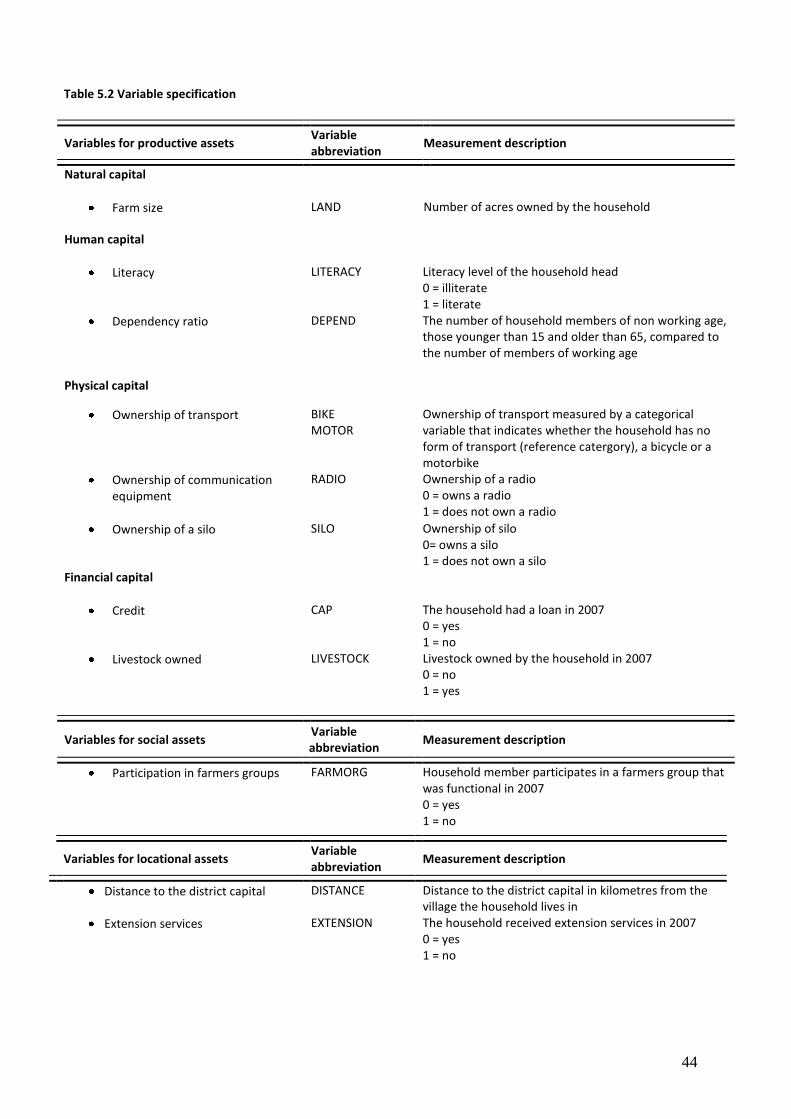
44

Variables for productive assets Variable abbreviation

Measurement description

Natural capital

Farm size LAND Number of acres owned by the household

Human capital

Literacy LITERACY Literacy level of the household head 0 = illiterate 1 = literate

Dependency ratio DEPEND The number of household members of non working age, those younger than 15 and older than 65, compared to the number of members of working age

Physical capital

Ownership of transport BIKE MOTOR

Ownership of transport measured by a categorical variable that indicates whether the household has no form of transport (reference catergory), a bicycle or a motorbike

Ownership of communication equipment

RADIO Ownership of a radio 0 = owns a radio 1 = does not own a radio

Ownership of a silo SILO Ownership of silo 0= owns a silo 1 = does not own a silo

Financial capital

Credit CAP The household had a loan in 2007 0 = yes 1 = no

Livestock owned

LIVESTOCK Livestock owned by the household in 2007 0 = no 1 = yes

Variables for social assets Variable abbreviation

Measurement description

Participation in farmers groups FARMORG Household member participates in a farmers group that was functional in 2007 0 = yes 1 = no

Variables for locational assets Variable abbreviation

Measurement description

Distance to the district capital DISTANCE Distance to the district capital in kilometres from the village the household lives in

Extension services EXTENSION The household received extension services in 2007 0 = yes 1 = no

Table 5.2 Variable specification

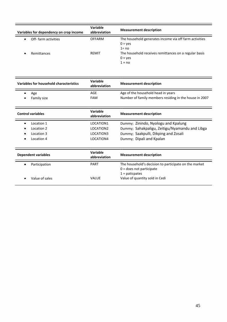
45

Variables for dependency on crop income

Variable abbreviation

Measurement description

Off- farm activities OFFARM The household generates income via off farm activities 0 = yes 1= no

Remittances REMIT The household receives remittances on a regular basis 0 = yes 1 = no

Variables for household characteristics Variable abbreviation

Measurement description

Age AGE Age of the household head in years

Family size FAM Number of family members residing in the house in 2007

Control variables Variable abbreviation

Measurement description

Location 1 LOCATION1 Dummy; Zinindo, Nyologu and Kpalung

Location 2 LOCATION2 Dummy; Sahakpaligu, Zeitigu/Nyamandu and Libga Location 3 LOCATION3 Dummy; Saakpulli, Dikping and Zosali Location 4 LOCATION4 Dummy; Dipali and Kpalan

Dependent variables Variable abbreviation

Measurement description

Participation PART The household’s decision to participate on the market 0 = does not participate 1 = paticpates

Value of sales VALUE Value of quantity sold in Cedi

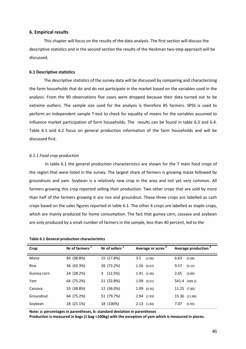
46

6. Empirical results

This chapter will focus on the results of the data analysis. The first section will discuss the

descriptive statistics and in the second section the results of the Heckman two-step approach will be

discussed.

6.1 Descriptive statistics

The descriptive statistics of the survey data will be discussed by comparing and characterizing

the farm households that do and do not participate in the market based on the variables used in the

analysis. From the 90 observations five cases were dropped because their data turned out to be

extreme outliers. The sample size used for the analysis is therefore 85 farmers. SPSS is used to

perform an independent sample T-test to check for equality of means for the variables assumed to

influence market participation of farm households. The results can be found in table 6.3 and 6.4.

Table 6.1 and 6.2 focus on general production information of the farm households and will be

discussed first.

6.1.1 Food crop production

In table 6.1 the general production characteristics are shown for the 7 main food crops of

the region that were listed in the survey. The largest share of farmers is growing maize followed by

groundnuts and yam. Soybean is a relatively new crop in the area and not yet very common. All

farmers growing this crop reported selling their production. Two other crops that are sold by more

than half of the farmers growing it are rice and groundnut. These three crops are labelled as cash

crops based on the sales figures reported in table 6.1. The other 4 crops are labelled as staple crops,

which are mainly produced for home consumption. The fact that guinea corn, cassava and soybean

are only produced by a small number of farmers in the sample, less than 40 percent, led to the

Table 6.1 General production characteristics

Note: a: percentages in parentheses, b: standard deviation in parentheses Production is measured in bags (1 bag =100kg) with the exception of yam which is measured in pieces.

Crop Nr of farmers a

Nr of sellers a

Average nr acres b

Average production b

Maize 84 (98.8%) 15 (17.8%) 3.5 (2.06) 6.63 (5.68)

Rice 36 (42.3%) 26 (72.2%) 1.56 (0.67) 9.57 (9.15)

Guinea corn 24 (28.2%) 3 (12.5%) 1.41 (1.06) 2.65 (3.89)

Yam 64 (75.2%) 21 (32.8%) 1.09 (0.61) 541.4 (449.2)

Cassava 33 (38.8%) 12 (36.0%) 1.09 (0.36) 11.25 (7.80)

Groundnut 64 (75.2%) 51 (79.7%) 2.94 (1.93) 15.36 (11.86)

Soybean 18 (21.1%) 18 (100%) 2.13 (1.84) 7.07 (5.93)

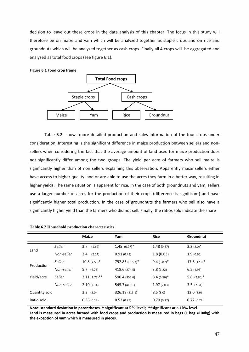
47

decision to leave out these crops in the data analysis of this chapter. The focus in this study will

therefore be on maize and yam which will be analyzed together as staple crops and on rice and

groundnuts which will be analyzed together as cash crops. Finally all 4 crops will be aggregated and

analysed as total food crops (see figure 6.1).

Figure 6.1 Food crop frame

Table 6.2 shows more detailed production and sales information of the four crops under

consideration. Interesting is the significant difference in maize production between sellers and non-

sellers when considering the fact that the average amount of land used for maize production does

not significantly differ among the two groups. The yield per acre of farmers who sell maize is

significantly higher than of non sellers explaining this observation. Apparently maize sellers either

have access to higher quality land or are able to use the acres they farm in a better way, resulting in

higher yields. The same situation is apparent for rice. In the case of both groundnuts and yam, sellers

use a larger number of acres for the production of their crops (difference is significant) and have

significantly higher total production. In the case of groundnuts the farmers who sell also have a

significantly higher yield than the farmers who did not sell. Finally, the ratios sold indicate the share

Table 6.2 Household production characteristics

Maize Yam Rice Groundnut

Land Seller 3.7 (1.62) 1.45 (0.77)* 1.48 (0.67) 3.2 (2.0)*

Non-seller 3.4 (2.14) 0.91 (0.43) 1.8 (0.63) 1.9 (0.96)

Production Seller 10.8 (7.55)*

5.7 (4.78)

792.85 (615.3)*

418.6 (274.5)

9.4 (3.87)*

3.8 (1.22)

17.6 (12.0)*

6.5 (4.93) Non-seller

Yield/acre Seller 3.11 (1.77)**

2.10 (2.14)

590.4 (355.6)

545.7 (418.1)

8.4 (5.56)*

1.97 (2.03)

5.8 (2.80)*

3.5 (2.31) Non-seller

Quantity sold 3.3 (2.0) 326.19 (213.1) 8.5 (8.0) 12.0 (8.9)

Ratio sold 0.36 (0.18) 0.52 (0.29) 0.70 (0.22) 0.72 (0.24)

Note: standard deviation in parentheses. * significant at 5% level; **significant at a 10% level. Land is measured in acres farmed with food crops and production is measured in bags (1 bag =100kg) with the exception of yam which is measured in pieces.

Total Food crops

Staple crops Cash crops

Rice Groundnuts

Maize Yam

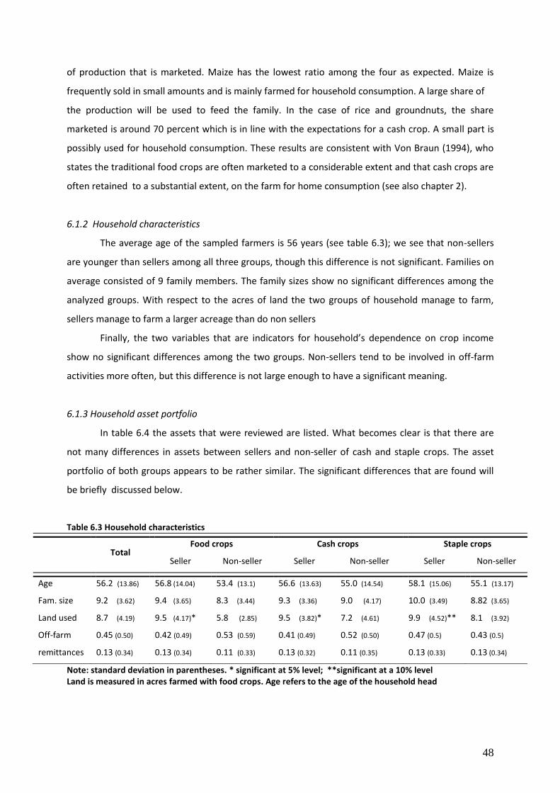
48

of production that is marketed. Maize has the lowest ratio among the four as expected. Maize is

frequently sold in small amounts and is mainly farmed for household consumption. A large share of

the production will be used to feed the family. In the case of rice and groundnuts, the share

marketed is around 70 percent which is in line with the expectations for a cash crop. A small part is

possibly used for household consumption. These results are consistent with Von Braun (1994), who

states the traditional food crops are often marketed to a considerable extent and that cash crops are

often retained to a substantial extent, on the farm for home consumption (see also chapter 2).

6.1.2 Household characteristics

The average age of the sampled farmers is 56 years (see table 6.3); we see that non-sellers

are younger than sellers among all three groups, though this difference is not significant. Families on

average consisted of 9 family members. The family sizes show no significant differences among the

analyzed groups. With respect to the acres of land the two groups of household manage to farm,

sellers manage to farm a larger acreage than do non sellers

Finally, the two variables that are indicators for household’s dependence on crop income

show no significant differences among the two groups. Non-sellers tend to be involved in off-farm

activities more often, but this difference is not large enough to have a significant meaning.

6.1.3 Household asset portfolio

In table 6.4 the assets that were reviewed are listed. What becomes clear is that there are

not many differences in assets between sellers and non-seller of cash and staple crops. The asset

portfolio of both groups appears to be rather similar. The significant differences that are found will

be briefly discussed below.

Table 6.3 Household characteristics

Total

Food crops Cash crops Staple crops

Seller Non-seller Seller Non-seller Seller Non-seller

Age 56.2 (13.86) 56.8 (14.04) 53.4 (13.1) 56.6 (13.63) 55.0 (14.54) 58.1 (15.06) 55.1 (13.17)

Fam. size 9.2 (3.62) 9.4 (3.65) 8.3 (3.44) 9.3 (3.36) 9.0 (4.17) 10.0 (3.49) 8.82 (3.65)

Land used 8.7 (4.19) 9.5 (4.17)* 5.8 (2.85) 9.5 (3.82)* 7.2 (4.61) 9.9 (4.52)** 8.1 (3.92)

Off-farm 0.45 (0.50) 0.42 (0.49) 0.53 (0.59) 0.41 (0.49) 0.52 (0.50) 0.47 (0.5) 0.43 (0.5)

remittances 0.13 (0.34) 0.13 (0.34) 0.11 (0.33) 0.13 (0.32) 0.11 (0.35) 0.13 (0.33) 0.13 (0.34)

Note: standard deviation in parentheses. * significant at 5% level; **significant at a 10% level Land is measured in acres farmed with food crops. Age refers to the age of the household head

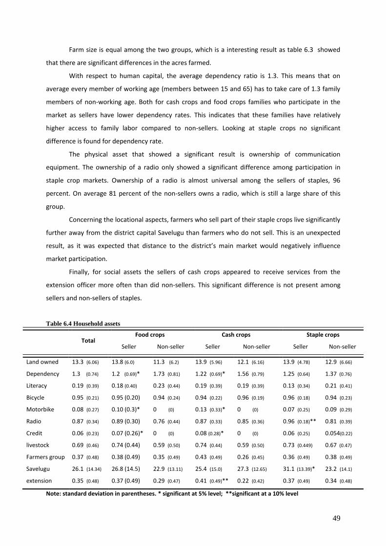
49

Farm size is equal among the two groups, which is a interesting result as table 6.3 showed

that there are significant differences in the acres farmed.

With respect to human capital, the average dependency ratio is 1.3. This means that on

average every member of working age (members between 15 and 65) has to take care of 1.3 family

members of non-working age. Both for cash crops and food crops families who participate in the

market as sellers have lower dependency rates. This indicates that these families have relatively

higher access to family labor compared to non-sellers. Looking at staple crops no significant

difference is found for dependency rate.

The physical asset that showed a significant result is ownership of communication

equipment. The ownership of a radio only showed a significant difference among participation in

staple crop markets. Ownership of a radio is almost universal among the sellers of staples, 96

percent. On average 81 percent of the non-sellers owns a radio, which is still a large share of this

group.

Concerning the locational aspects, farmers who sell part of their staple crops live significantly

further away from the district capital Savelugu than farmers who do not sell. This is an unexpected

result, as it was expected that distance to the district’s main market would negatively influence

market participation.

Finally, for social assets the sellers of cash crops appeared to receive services from the

extension officer more often than did non-sellers. This significant difference is not present among

sellers and non-sellers of staples.

Table 6.4 Household assets

Total

Food crops Cash crops Staple crops

Seller Non-seller Seller Non-seller Seller Non-seller

Land owned 13.3 (6.06) 13.8 (6.0) 11.3 (6.2) 13.9 (5.96) 12.1 (6.16) 13.9 (4.78) 12.9 (6.66)

Dependency 1.3 (0.74) 1.2 (0.69)* 1.73 (0.81) 1.22 (0.69)* 1.56 (0.79) 1.25 (0.64) 1.37 (0.76)

Literacy 0.19 (0.39) 0.18 (0.40) 0.23 (0.44) 0.19 (0.39) 0.19 (0.39) 0.13 (0.34) 0.21 (0.41)

Bicycle 0.95 (0.21) 0.95 (0.20) 0.94 (0.24) 0.94 (0.22) 0.96 (0.19) 0.96 (0.18) 0.94 (0.23)

Motorbike 0.08 (0.27) 0.10 (0.3)* 0 (0) 0.13 (0.33)* 0 (0) 0.07 (0.25) 0.09 (0.29)

Radio 0.87 (0.34) 0.89 (0.30) 0.76 (0.44) 0.87 (0.33) 0.85 (0.36) 0.96 (0.18)** 0.81 (0.39)

Credit 0.06 (0.23) 0.07 (0.26)* 0 (0) 0.08 (0.28)* 0 (0) 0.06 (0.25) 0.054(0.22)

livestock 0.69 (0.46) 0.74 (0.44) 0.59 (0.50) 0.74 (0.44) 0.59 (0.50) 0.73 (0.449) 0.67 (0.47)

Farmers group 0.37 (0.48) 0.38 (0.49) 0.35 (0.49) 0.43 (0.49) 0.26 (0.45) 0.36 (0.49) 0.38 (0.49)

Savelugu 26.1 (14.34) 26.8 (14.5) 22.9 (13.11) 25.4 (15.0) 27.3 (12.65) 31.1 (13.39)* 23.2 (14.1)

extension 0.35 (0.48) 0.37 (0.49) 0.29 (0.47) 0.41 (0.49)** 0.22 (0.42) 0.37 (0.49) 0.34 (0.48)

Note: standard deviation in parentheses. * significant at 5% level; **significant at a 10% level

50

Several of the assets appeared not to be suitable to use in further analysis due to the limited

number of scores on either sellers or non-sellers. This counts for the ownership of a motorbike,

ownership of a bicycle and credit. In the case of bicycle the problem occurred in the situation of

people not having a bicycle which is an exception. For the ownership of a motorbike and the access

to credit a limited number of people scored positive on them. Due to this there is no variance

measured in these variables which causes problems with the estimation of the Probit model that is

performed in the Heckman two-step approach. That is way these variables are dropped from the

analysis

6.2 Econometric results

In table 6.5, the regression results for market participation and value of sales are shown.

There are three regression models, (I) the log of total sales of food crops, (II) the log of staple crop

sales and (III) the log of cash crop sales. For each model the results of the conditional equation, the

log value of sales given market participation are reported in the first column, and the results of the

selection equation, the market participation decision of the household, are shown in the second

column.

The Heckman two-step approach is based on the assumption that the selection equation and

the conditional equation are related to each other through their error terms. When there is no

relation between the error terms there is no need to perform an Heckman two step approach as

there is no sample selection bias and an OLS regression will give unbiased estimators. The correlation

between the error terms is indicated in table 6.5 by the selectivity parameter, ρ. The correlation for

all three models is large, indicating that there is a selection bias. The selectivity parameter is

significant in the regressions for total food crops and for staple crops, which indicates that the two

equations are not independent from each other through the correlation of the error terms. This

parameter is non-significant in the case of the model for cash crops. Due to this, the second stage of

the Heckman two-step approach with respect to cash crops cannot be interpreted. For that reason a

OLS regression without Heckman’s lambda has been performed. The results of this test can be found

in Annex IV.

The Heckman’s lambda is included in the regression to control for the influence of

unobserved characteristics on market participation. The regression coefficient of the control factor is

an indicator for the covariance of the error terms. In all three models the control factor is non-

significant.

In the model there are several potentially endogenous variables included. Endogeneity refers

to the fact that an independent variable included in the model is potentially a choice variable which

is determined by other variables that are as well included in the model: Off farm labour, extension

51

services and farm group membership. Due to this it is not possible to infer causality with respect to

these variables. They are kept in the model, because they represent assets that are of interest in this

research. An extra regression has been performed on each model without the endogenous variables.

The results will be briefly discussed at the end of this chapter in section 6.2.4 and the outputs can be

found in Annex V.

6.2.1 Total food crops

The Probit model results for total sales of food crops indicate that besides the location

dummy 4 only the human capital asset, log dependency rate shows a negative significant effect on

the market participation decision of small holder farmers. This indicates that families with higher

dependency rates are less likely to participate on the market as sellers. They have relatively less

labour in their households than their counterparts with low dependency rates. This suggest that

labour availability in the household is an important factor in the market participation decision. None

of the variables representing social or locational assets had a significant effect on the participation of

smallholder farmers in food crop markets as sellers. The location dummy 4 shows a negative

significant effect which is associated with the weather conditions of 2007. Many farmers reported

large production losses in this region which impacts their market participation.

In the second stage, OLS results show that financial capital in the form of ownership of

livestock, is the only private asset that has a positive significant effect on the degree of participation.

Livestock can be seen as the household’s savings account, in case of crop failure households with

livestock can financially rely on their livestock. This enables them to take more risks which according

to the results leads to higher volumes of sale on the market. Locational nor social assets appeared to

have a significant effect on the sales volumes of smallholder farmers. Among the non-asset

household characteristics, the age of the household head has a negative significant effect on the

volume of sales. This negative relationship between age and degree of participation could be

explained by the conservative attitude of older farm household heads. The participation in markets

by older household heads could be explained by the fact that many households are engaged in some

for of trade, to assure their need for cash or products they do not produce themselves. But their

conservative attitude restrains them to move away from their subsistence oriented farming method

towards market orientation and an increased degree of participation. The location dummy 4 also

shows a significant negative relationship for the degree of participation. The same explanation as

given above counts for this result.

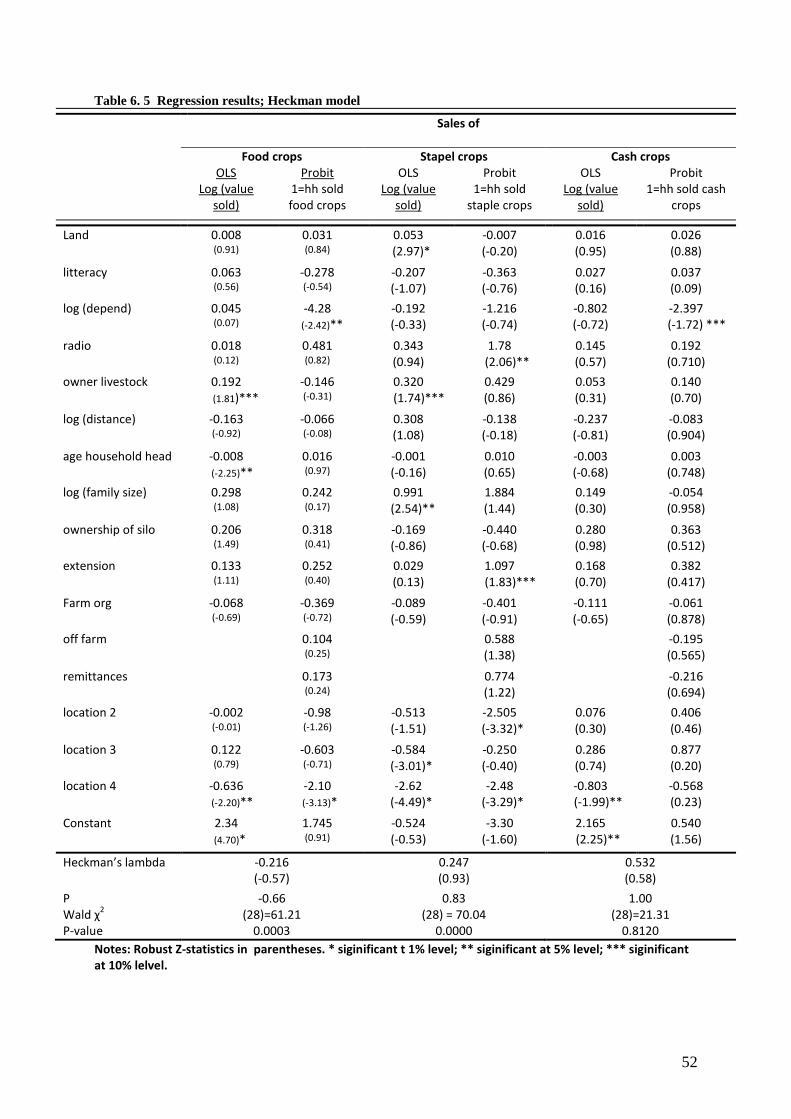
52

Table 6. 5 Regression results; Heckman model

Sales of

Food crops Stapel crops Cash crops OLS

Log (value sold)

Probit 1=hh sold food crops

OLS Log (value

sold)

Probit 1=hh sold

staple crops

OLS Log (value

sold)

Probit 1=hh sold cash

crops

Land 0.008 (0.91)

0.031 (0.84)

0.053 (2.97)*

-0.007 (-0.20)

0.016 (0.95)

0.026 (0.88)

litteracy 0.063 (0.56)

-0.278 (-0.54)

-0.207 (-1.07)

-0.363 (-0.76)

0.027 (0.16)

0.037 (0.09)

log (depend) 0.045 (0.07)

-4.28 (-2.42)**

-0.192 (-0.33)

-1.216 (-0.74)

-0.802 (-0.72)

-2.397 (-1.72) ***

radio 0.018 (0.12)

0.481 (0.82)

0.343 (0.94)

1.78 (2.06)**

0.145 (0.57)

0.192 (0.710)

owner livestock 0.192 (1.81)***

-0.146 (-0.31)

0.320 (1.74)***

0.429 (0.86)

0.053 (0.31)

0.140 (0.70)

log (distance) -0.163 (-0.92)

-0.066 (-0.08)

0.308 (1.08)

-0.138 (-0.18)

-0.237 (-0.81)

-0.083 (0.904)

age household head -0.008 (-2.25)**

0.016 (0.97)

-0.001 (-0.16)

0.010 (0.65)

-0.003 (-0.68)

0.003 (0.748)

log (family size) 0.298 (1.08)

0.242 (0.17)

0.991 (2.54)**

1.884 (1.44)

0.149 (0.30)

-0.054 (0.958)

ownership of silo 0.206 (1.49)

0.318 (0.41)

-0.169 (-0.86)

-0.440 (-0.68)

0.280 (0.98)

0.363 (0.512)

extension 0.133 (1.11)

0.252 (0.40)

0.029 (0.13)

1.097 (1.83)***

0.168 (0.70)

0.382 (0.417)

Farm org -0.068 (-0.69)

-0.369 (-0.72)

-0.089 (-0.59)

-0.401 (-0.91)

-0.111 (-0.65)

-0.061 (0.878)

off farm

0.104 (0.25)

0.588 (1.38)

-0.195 (0.565)

remittances

0.173 (0.24)

0.774 (1.22)

-0.216 (0.694)

location 2 -0.002 (-0.01)

-0.98 (-1.26)

-0.513 (-1.51)

-2.505 (-3.32)*

0.076 (0.30)

0.406 (0.46)

location 3 0.122 (0.79)

-0.603 (-0.71)

-0.584 (-3.01)*

-0.250 (-0.40)

0.286 (0.74)

0.877 (0.20)

location 4 -0.636 (-2.20)**

-2.10 (-3.13)*

-2.62 (-4.49)*

-2.48 (-3.29)*

-0.803 (-1.99)**

-0.568 (0.23)

Constant 2.34 (4.70)*

1.745 (0.91)

-0.524 (-0.53)

-3.30 (-1.60)

2.165 (2.25)**

0.540 (1.56)

Heckman’s lambda -0.216 (-0.57)

0.247 (0.93)

0.532 (0.58)

Ρ -0.66 0.83 1.00 Wald χ

2 (28)=61.21 (28) = 70.04 (28)=21.31

P-value 0.0003 0.0000 0.8120

Notes: Robust Z-statistics in parentheses. * siginificant t 1% level; ** siginificant at 5% level; *** siginificant at 10% lelvel.

53

6.2.2 Staple crops

For the decision to participate in the market of staple crops as a seller the Probit results

indicate that the physical asset in the form of radio ownership has a positive significant effect on

market participation. The ownership of a radio is associated with wealth, which enables farmers to

invest more in their farms. This corresponds with the positive relation found for radio ownership. For

locational assets, the access to extension services showed a positive significant effect. No significant

effect were found for non-asset household characteristics. The location dummies 2 and 4 were

significant. For location 4 the weather conditions played an important role in the participation in

staple crop markets as well. Location 2 also showed a negative relation to market participation. This

could be the result of the higher population pressure which is assumed to influence soil fertility. This

in turn impacts the yield and the market participation opportunities of the household.

The results of the second stage OLS shows that for privately held assets, natural capital in the

form of farm size has a positive significant effect on the volume of staple crop sales. This is in

correspondence with the expectation that farm households with more access to land can produce

more which leads to a higher volume of sales. A positive relationship is also found for financial capital

measured by the ownership of livestock. The same explanation as given under total food crops

counts here for this variable. For social assets no significant effect was found. With respect to the

non-asset household characteristics, family size of the household showed a positive significant effect

on the volume of sales. This sign is unexpected as it indicates that families with more members are

selling larger quantities than small families do. A possible explanation is that the larger families have

a higher availability of labour compared to smaller families, but at the same time all these mouths

have to be filled, making this result difficult to explain. The dummies for location 3 and 4 showed

negative significant effects as well. Location 3 represents the northern area of the district. The

weather problems were not described as more severe here than in the eastern and central area. The

northern area of the district is more remote than the other parts which might be a possible

explanation for the negative relation to degree of participation. For location 4 the weather impact

remains the most likely explanation for the lower degree of participation.

6.2.3 Cash crops

The results of the Probit analysis for cash crop market participation show only a negative

significant effect for the human capital asset, dependency ratio. The other assets did not have a

significant effect on the decision to participate in the market of cash crops. No significant effects

were found for non-asset household characteristic or location dummies.

The second stage OLS for cash crops is non-significant. The variables included do not predict

the outcome well. Therefore, no indications can be made about the variables included in the model.

54

6.2.4 Model 2

In the analysis without the endogenous variables (see Annex V) the results came out rather

similar compared to the original model. With respect to staple crops the ownership of livestock

shows no longer a significant effect on the volume of sales and for cash cops non of the variables

showed a significant effect in the Probit results. For the model of food crops the results remained the

same.

55

7. Constraints faced by smallholder farmers

This chapter will discuss the different constraints that came up in the personal interviews

with farmers on their possibilities to increase the participation in food crop markets e.g. sell larger

volumes of food crops at the market. A distinction is made between the limitations that the farmers

pointed out themselves and the constraints that were observed during the discussions with them.

7.1 Introduction

“How can we sell if we barely produce enough to feed ourselves”, this is a statement often

made by the interviewed farmers when discussing their market participation. The farmers face the

problem that their production is not high enough to “seriously” participate in the market. Currently

they sell small portions of their yield whenever there is an urgent need for money. This should be

placed in perspective, as 75 percent of the interviewed farmers produces groundnuts (15 bags on

average) of which a large proportion is marketed (9 bags on average). The same holds for rice

production. The difference with groundnuts though is that a relatively small number of farmers

grows rice, 42 percent. For staples the story is rather different. Only a few households, 17 percent,

indicated to sell a part of their maize yield. Over half of them did this out of necessity in order to

cover the costs faced at that moment and they had to purchase maize at a later moment from the

market again to be able to feed their families. This situation might be different in other years as this

year’s yields were low due to weather circumstances.

Maize is the most important crop for the Dagombas and 75 percent of the farmers indicated

that this is the crop they want to produce more if they had the means to do so. The reasoning behind

this is “that maize is what they eat”. As a farmer said: “You have to be satisfied before you can get

rich”. After the family is provided with enough maize one can focus on other crops. Of these farmers

80 percent indicated that they wanted to produce more maize for their own consumption, in case

there would be something left they could sell it to a trader. Planned production of maize for the

market is apparently not a possibility or a priority at this moment.

A clear distinction could be made between farmers who prefer to grow crops they can

consume in case the maize harvest is low and farmers who dare to take a market risk and produce

cash crops which need to be sold on the market and buy staples in return. Farmers belonging to the

first group can be seen as the traditional subsistence-oriented farmers while the second group could

potentially move towards the more market-oriented subsistence farmer. The distinction between

these two groups was related to the age of the household heads. The older household heads more

often wanted to focus on traditional staples and appeared more conservative than their younger

counterparts who were willing to look for new opportunities. This last group is rather small though.

Enough ideas on what to do and produce but which constraints keep them from doing so?

56

7.2 Perceived constraints by smallholder farmers

“It’s the money stupid!”, the lack of financial means is the most heard explanation of the

farmers for their lack of expansion or ability to make changes on their farm in order to increase their

participation in food crop markets. If they had the money they could ask the tractor services (or in

some places the oxen) to plough more land for them, they could buy fertilizer (for cereal production:

maize and rice) so the crops would grow better and they could hire labour for weeding (especially

necessary for cereal production). There are several factors named by the farmers that can be linked

to the lack of financial means. These will be briefly discussed below.

7.2.1 Financial constraints

Almost 75 percent of the farmers in the district make use of tractor services to plough most

of their fields. Over the years these farmers have seen tractor prices increase sharply due to

increasing fuel prices and the pressure on the tractor services. Prices for an acre were at the

beginning of the farming season 20 Cedi per acre compared to 16 Cedi per acre last year, with the

prices of this year still rising. As soon as the first rains come there is a high demand for tractor

services, leaving a number of farmers waiting for a long time before they can start preparing their

lands, while timing is essential in rain fed agriculture.

As an alternative an oxen plough could be used. But also the cost of hiring this service has

risen at the same pace as the tractor service, though it remains a little cheaper. The biggest

disadvantage of using oxen is that it is slow and time is precious. The lands need to be prepared on

time, forcing some of them to use tractor services after they started with the oxen. In certain areas

with big soil fertility problems the oxen plough is the preferred method as with oxen you only plough

the top layer. Unfortunately not many people offer services for the oxen plough and farmers

indicated not to be able to afford their own pair of oxen.

The decline in soil fertility is noticed everywhere in the district. Soil fertility is always named

together with the fact that they can’t afford fertilizer. The farmers indicate that they would like to

use fertilizer on their cereals especially on their maize and in lesser extent on their rice. Last year 27

percent of the farmers used fertilizer, although often in lower quantities than recommended. Prices

have gone skyrocketing, for many the price of 20 Cedi per bag last year was already too costly and

with the price of a bag of fertilizer risen to 40 Cedi not many will have the opportunity to buy any

coming season.

All the households interviewed indicated that the labour delivered by the household is not

sufficient for the farming activities and so labour from outside is needed. Most needed is labour for

weeding, though this is not universal for all crops as for yam and cassava most labour is needed

preparing the land which can only be done by hand. Labour shortage at time of sowing is overcome

57

by using children from the community and during harvest and weeding communal labour is often

used. The disadvantage of communal labour is that the men only work one day on a farmer’s land

and often the work is not finished at the end of the day. To finish tasks on time labour needs to be

hired. There appears to be no shortage of labour on the labour market, all farmers indicated that if

they wanted to use external labour they had no problem finding it. In Dipali they explained that

especially people from Upper East come to the Northern region to earn some extra money as their

lands are very bad. Slightly less than 50 percent of the farmers did not have the finances to hire in

labour last year. The fact that labour is already needed to farm the current acreage will make

external labour more important in case of expansion or intensification.

Another financial problem that was mentioned was the high costs associated with yam and

cassava seeds. Due to the bad harvest of last year, several farmers did not get enough seeds to

continue production or had to reduce the number of acres planted. The seeds for these crops are

rather expensive in comparison to the others crops, limiting the acres that will planted with them.

Cost of clearing land is often mentioned as an argument that prevents farmers from

increasing production. Over half of the farmers indicated that clearing land was very important if

they wanted to scale up their production. It appeared not to be a problem to find this land. Either

there was family land still being available or community land that could be accessed. Though land

might seem to be available, the question is what type of land they have access to. I have

encountered farmers that wanted to expand the number of acres with rice, but the area with

swampy lowland was completely used and so constrained them in doing so.

7.2.2 Credit

To overcome the lack of financial means one could consider taking a loan. Unfortunately, the

credit options of the farmers appear to be minimal in this area, especially credit that can be used for

food crop production. There are quite some credit organizations based in Tamale that operate in the

surrounding districts, like Savelugu-Nanton. These organisations often have credit schemes for safer

activities like processing rice or producing Shea-butter. The credit that is available for farming

activities is often only provided for cash crops like rice and soybeans and not for the most important

crops maize and yam. This leads to tension between farmers preferences and the NGO’s interest.

Besides that the credit that is available to farmers often has the condition attached that the

farmers should group themselves first. This leads to the exclusion of certain groups of farmers.

Several farmers reported being too late to join a group as there is a fixed number of participants per

village, others reported that the indigenous often cut of settlers from benefiting from such

opportunities and it is mentioned that the “better off” of the village are often the ones “asked” for

the groups, restricting financial opportunities for others.

58

Few of the farmers spoken with, 6 percent, had a loan (In the form of cash) at the time of the

interview. Not only due to the limited availability but also due to the perceived risks associated with

taking a loan. Many fear the risk of becoming indebted through the risk involved in rain-fed farming

and give examples of neighbours who had difficulties in the past with repaying and ended up losing

some of their assets which made them worse off, making them afraid of taking a loan.

Another often mentioned problem is the timing, as money is specifically needed at the start

of the farming season, credit institutes offer the money at less useful moments. This combined with

the relatively short repayment period make loans less attractive as well.

In the past several credit organisations operated in Savelugu Nanton for a fixed number of

years after which the farmers have to be able to manage themselves. The farmers that participated

in such programmes, of which the Lowland rice company is an important one, mention that they are

not able to maintain production at the same level as with the support. There is no active approach

towards finding new loan possibilities. People expect that eventually someone else will come to

support them as has happened over the last decennia.

7.3 Observed constraints

The farmers themselves came up with the limitations that they linked directly to their

production. Though in the conversations some other aspects came up that in my eyes indirectly can

have an impact on their production and market participation as well but were not named as such.

These personal observations are described below and focus on extension services, farmers groups

and trade.

7.3.1 Extension services

The extension service that the government delivers should educate farmers on improving

their farm methods. This can be helpful for farmers to make an extra step forwards towards

commercialisation. But extension services do not function well. Three of the selected villages have

not seen the officer for at least two years. Of the interviewed farmers only 30 indicated to have been

in contact with the extension officer in the year 2007. The farmers mentioned that the information

provided by the extension officer was mainly focussing on livestock rearing and disease prevention

instead of giving information related to crop production. Another complaint about the extension

services is that the methods that are taught are costly and not applicable for the small farmers. The

bigger farmers are said to be more often selected to join the extension officers visit. A note to this is

that even the low-external input farming techniques (compost, agro-forestry, increased manure use)

that are part of the conventional extension services, are seen by farmers as “techniques for the rich”.

59

What became clear is that the outreach is limited and that there is a gap between what is needed

and what is offered.

7.3.2 Farming groups

Self organisation in groups is common when it concerns communal labour groups. In every

community visited, male and female communal labour groups are present. Other local initiatives

mainly focus on the support of social occasions and not on farming related issues. Groups that do

focus on farming are founded by NGOs. Of the interviewed farmers, 32 where members of such

farmer groups.

“Forming farmer groups is only interesting if a stranger comes and does it for you, because it

means that there is something to get”; this statement was made by a farmer in Kpalan and describes

the general feeling towards groups very well. A regular given explanation for the lack of local

initiatives is that forming groups without external help only leads to endless discussions, fights and

high costs.

The interviewed farmers appeared to be sceptical towards the working of farming-related

groups. Common arguments focussed on their concern that groups cannot work as every farm

household works in a different way. These concerns mainly focus on the idea that they should buy

inputs and sell their yields at the same time. Another often referred problem is that groups set up on

demand of NGOs frequently do not get the help that they were promised. Farmers get suspicious as

they have been disappointed too many times. Groups that do function are, according to the farmers

interviewed in Dipali, often dominated by the enlightened (ones that had been to school), preventing

others to profit from it. The contradiction with regard to farmer groups is that on the hand farmers

are disappointed by situations from the past and do not fancy groups but on the other hand do wait

for organisations to come and arrange things for them.

7.3.3 Trade

Marketing the crops is the last step that need to be taken. Among the interviewed farmers

only 6 percent took their produce to the market themselves. These farmers indicated that they could

not wait any longer for the traders to buy their produce at the farm gate. It is common in this area to

sell produce to traders who visit the villages on market days. All the selected villages had traders

visiting them. Though prices paid by these traders are lower than they are at the markets, there is no

incentive among the farmers to take the effort to go there. Farmers are well aware of the price levels

of their products in the region they live. This information is broadcasted on radio programs. Besides

that, going to the market is seen as a social activity especially for the youngsters. They will bring

60

information about the prices home. If there is nobody from your family going, there is always a

neighbour who is able to inform you.

Going to the market is time consuming, costly and risky. Combined with the fact that most

farmers sell only small quantities makes going to the market yourself not efficient. Price levels

between farm gate and market are not very different. The position of the traders is an interesting

one. It looks like they have quite a lot of power compared to the farmers. Organisation among

farmers to sell together in order to overcome the costs of transport is, as explained under farm

groups not common.

7.4 Conclusion

Maintaining the current levels of production is already difficult for the farmers, not to

mention increasing production. Planned production for the market is currently not their priority. The

focus of the farmers lies on securing the consumptive needs of the farm household by producing

enough maize before concerning additional activities. The state of mind of the farmers is still that of

the subsistence-oriented producer. The lack of financial means are according to the farmers their

biggest constraint preventing them from moving forward. Without money, the costs associated with

expansion (like increased labour costs, fertilizer expenses etc.) cannot be made. Though their need

for money does not equal their demand for credit. Taking a loan is taking a risk which many do not

dare to make, being afraid of loosing the assets that they have. Besides that, credit opportunities for

crop production are limited making it more difficult to get access to financial means.

61

8. Conclusion

The Ghana School Feeding Program aims at raising smallholder farmers income and reducing

poverty among them by the use of a market-based development strategy. Markets can only

stimulate wealth creation among those who can afford to participate in them. The aim of this

research is to analyze the impact of the asset portfolio of smallholder farmers on market

participation in food crop markets.

In Savelugu-Nanton the majority of farmers is engaged in the production of staple crops at

the subsistence level. In the long run subsistence farming is assumed not to be a viable activity for

safeguarding household security and welfare. The process of commercialisation is seen as essential

for the reduction of poverty and improvement of food security. In the process of commercialisation a

distinction is made between subsistence farmers who are subsistence oriented producers, standing

at the beginning of the commercialisation process and market oriented subsistence farmers who are

moving towards the state of semi-commercial farmers. The asset endowment of farm households

plays an important role as it determines the opportunity set of the household. The allocation of the

assets creates the household’s production opportunities and their livelihood strategy.

The empirical analysis of the three models under consideration, (I) total sales of food crops,

(II) staple crop sales and (III) cash crop sales shows that the asset portfolio of the farm household has

little impact on their market participation behavior. The statistical comparison indicated that the

asset endowment among the sellers and non-sellers was very similar and in the econometric analysis

little evidence was found for asset-related barriers for crop market entrance and volume of sales.

The asset barriers that were found are:

Crop market entrance

Total food crops; the dependency ratio

Staple crops; the ownership of a radio

Cash crops; the dependency ratio

Degree of participation

Total food crops; ownership of livestock

Staple crops; the ownership of livestock and farm size

The locational asset, access to extension services only appeared to have an influence on the market

participation decision in staple crop markets and social assets appeared not to form a barrier in any

of the models.

Though the assets among sellers and non-sellers appeared similar the sellers are able to farm

significantly more land. This clearly marks a difference in the potential between the two groups. This

result cannot be explained by the data collected in this research and should be looked at in further

research.

62

The farmers perceive their lack of financial means as their biggest constraint. Currently their

production levels are low. They are subsistence oriented producers that do not have the ability to

plan production for the market. In order for these farmers to benefit from market-based

development strategies they need to expand or intensify their production to move towards the

market oriented stage. Financial constraints limit the farmers from doing so at this moment. Though

their need for money does not equal their demand for credit as they do not dare to take the risk

associated with credit. There appears to be a status quo. Opportunities to push development could

be found in the improvement of the functioning and general understanding of extension services,

farming groups and the trading position of the farmers. At this moment these appear to be

underdeveloped. Another option is to offer additional services within the Ghana School Feeding

Program that will help the farmers make the necessary investments during the farming season and

lift up their production levels.

8.1 Limitations

The interviews took place at the start of the farming season. Causing many of the household

heads to be away from their houses. At the start of the season there is also a group of

farmers who for various reasons decided to postpone farming activities until later. To get a

sample which contained both groups of farmers the interviews, when possible, took place

during the afternoon when most farmers returned to rest and look for shelter from the sun.

Still there is a change that there is a overrepresentation of farmers that started farming later

in the season causing a bias in the sample.

The data were collected over the year 2007. This year the weather conditions were

extremely bad. Absence of rain at the start of the farming season caused seeds not to

germinate and the heavy showers just before harvest destroyed a large share of the crops.

Households that lived near the river Volta were worst off as their villages and farm lands

flooded after the showers. The production levels have been influenced due to these weather

circumstances and have an impact on the choices made by the farm household with regard

to their market participation. That is why the data should be interpreted with caution.

This research primarily focused on the selling of food crops on the market. It does not take

into account selling and re-buying behavior. Households that sell after harvest an re-buy the

same product later in the season influence the results as these farmers might not be net

sellers but are marked in this study as such. This might have caused the results to show

63

limited differences in asset portfolios of sellers and non-sellers Further research should take

this behavior into account.

The analysis is performed on three models which look at the aggregate of crops. By using

aggregates supply the individual differences in the underlying causal mechanisms related to

individual crop decisions are hidden. To get a complete overview of asset barriers to food

market participation single crop estimations should be added.

The access to credit has not been incorporated in the model. From the interviews it became

clear that the lack of financial means are seen as the biggest constraint for farmers to expand

their production. That is why it might be important to include this variable in the model. The

variable access to credit was not correctly measured in this study and the data collected

could therefore not be used. Access to credit was measured with the question whether a

farm household accessed a loan in 2007 or not. The answers in the first place only

concentrated on credit in the form of direct cash flows and not with respect to the provision

of inputs or services. Secondly this does not measure in a correct way the access to credit by

households as there are households who do have access, but do not take a loan. This should

be taken into account in further research.

64

9. References

Al-Hassan, R. M. & X. Diao (2007). Regional disparities in Ghana: Policy options and public investment implications. IFPRI Discussion Paper 693. Washington, D.C. International Food Policy Research Institute (IFPRI).

Barrett, C.B. (2008). Smallholder market participation: Concept and evidence from eastern and southern Africa. Food Policy, 33, 299-317.

Benfica, R.M.S. & D.L. Tschirley & D.H. Boughton (2006). Interlinked transactions in cash cropping

economies: The determinants of farmer participation and performance in the Zambezi river valley of Mozambique. Contributed paper presented at the 26 International Association of Agricultural Economists Conference, Gold Coast, Australia, August 12-18, 2006.

Benin, S., T. Mogues, g. Codjoe, J. Randriamamonly (2008). Reaching middle-income status in Ghana

by 2015: Public expenditures anad agricultural growth. IFPRI Discussion Paper 00811. Washington, D.C. International Food Policy Research Institute (IFPRI).

Boughton, D., D. Mather, C.B. Barrett, R. Benfica, D. Abdula, D. Tschirley, B. Cunguara (2007). Market

participation by rural households in a low-income country: An asset based approach applied to Mozambique. Faith and Economics, 50, 64-101

Breisinger, C. & X. Diao & J. Thurlow & R.M. Al-Hassan (2008). Agriculture for development in Ghana:

New opportunities and Challenges. IFPRI Discussion Paper 00784. Washington, D.C. International Food Policy Research Institute (IFPRI).

Brounstein, D., D. Mayer, J. Shia & P. Hwong (2006). Opportunities for sustainable development of

the Ghana School Feeding Programme through agricultural empowerment. International Business Development Program, University of California, Berkeley: in Collaboration with the United Nations Hunger Task Force.

Brüntrup, M. & F. Heidhues (2002). Subsistence agriculture in development: Its role in process of

structural change. Research in Development Economics and Policy, Discussion Paper No. 1/2002. Institute of Agricultural Economics and Social Sciences in the Tropics and Subtropics, University of Hohenheim.

Codjoe, S.N.A. (2007). Supply and utilisation of food crops in Ghana, 1960-2000. African Journal of

Food, Agriculture, Nutrition and Development, 7 (2), 1-15.

De Janvry, A., M. Fafchamps & E. Sadoulet (1991). Peasant household behaviour with missing markets: Some paradoxes explained. Economic Journal, 101, 1400-1417.

De Janvry, A. & E. Sadoulet (2006). Progress in the modelling of rural households' behavior under

market failures. In: A. de Janvry and R. Kanbur (eds). Poverty, Inequality and Development: Essays in Honor of Erick Thorbecke. Boston, MA: Springer.

W.H. Dow & Norton, E.C. (2003). Choosing between and interpreting the Heckit and two-part models

for corner solutions. Health Services & Outcomes Research Methodology, 4, 5-18. Ellis, F. (1988). Peasant Economics: Farm Households and Agrarian Development. Cambridge

University Press, Cambridge.

65

Fafchamps, M. (1992). Cash crop production, food price volatility and rural market integration in the Third-World. American Journal of Agricultural Economics, 74(1), 90-99.

Goetz, S.J. (1992). A selectivity model of household food marketing behaviour in Sub- Saharan Africa.

American Journal of Agricultural Economics, 74(2), 444-452. Ghana districts (2008). Savelugu Nanton. Available: www.ghanadistricts.com/districts (Accessed: 16-

10-2008). Ghana-net (200X). Map of Northern Ghana. Available: http://ghana-net.com/Documents/776px-Northern_Ghana_districts.bmp. (Accessed: 10-03-2008) GoG (2005). Support to NEPAD-CAADP Implementation, Volume I of III. National medium term

investment program. Government of Ghana, Accra. GoG (2006). Ghana School Feeding Programme, programme document 2007-2010. Government of

Ghana, Accra. Heltberg, R. & F. Tarp (2001). Agricultural supply response and poverty in Mozambique. WIDER

Discussion Paper No.2001-114. Helsinki, World Institute for Development Economic Research (WIDER).

ISSER (200X). Empowering farming communities in Northern Ghana with strategic innovations and

productive resources in dryland farming. Institute of Statistical and Economic Research Accra, Ghana. www.waterandfood.org/fileadmin/CPWF_Documents/Documents/First_call_projects/

PN6.pdf - Key, N., E. Sadoulet & A. de Janvry (2000). Transactions costs and agricultural household supply

response. American Journal of Agricultural Economics, 82(2), 245-259. Kostov, P. & J. Lingard (2004). Subsistence agriculture in transition economies: Its roles and

determinants. Journal of Agricultural Economics, 55(3), 565-579. Löfgren, H. & S. Robinson (1999). To trade or not to trade: Non-separable household models in

partial and general equilibrium. IFPRI Discussion Paper 37. Washington, D.C. International Food Policy Research Institute (IFPRI).

Manu-Aduening, J.A., R.I. Lamboll, G. Ampong Mensah, J.N. Lamptey, E. Moses, A.A. Dankyi & R.W.

Gibson (2006). Development of superior cassava cultivars in Ghana by farmers and scientists: The process adopted, outcomes and contributions and changed roles of different stakeholders. Euphytica, 150, 47-61.

Modern Ghana (2006). Northern region: Executive summary. Available:

www.modernghana.com/GhanaHome/regions/northern (Accessed: 15-10-2008) Moll, H., F. van der Staaij & A. van Tilburg (2001). Smallholders and markets, towards a conducive

environment. The Hague : Ministry of Foreign Affairs Moser, C. (2005). Assets, livelihoods and social policy. Conference paper prepared for the Arusha

Conference of the World Bank, “New Frontiers of Social Policy: Development in a Globalizing World”. Arusha Tanzania.

66

Nweke, F. (2004). New challenges in the cassava transformation in Nigeria and Ghana. IFRI Discussion Paper 118. Washington, D.C. International Food Policy Research Institute (IFPRI).

Pender, J. & D. Alemu (2007). Determinants of smallholder commercialization of food crops: Theory

and evidence from Ethiopia. IFPRI Discussion Paper No. 00745. Washington, D.C. International Food Policy Research Institute (IFPRI).

Pingali, P.H. (1997). From subsistence to commercial production systems: The transformation of

Asian agriculture. American Journal of Agricultural Economics, 79 (2), 628-634. Pingali, P.L & M.W. Rosegrant (1995). Agricultural commercialization and diversification: Processes

and policies. Food Policy, 20(3):171-186. Pingali, P., Y. Khwaja & M. Meijer (2005). Commercializing small farms; reducing transaction costs.

ESA Working Paper No. 05-08. Rome, The Food and Agriculture Organization (FAO). Sadoulet E. & A. de Janvry (1995). Quantitative Development Policy Analysis. The John Hopkins

University Press, Baltimore and London. Siegel, P.B. & J. Alwang (1999). An asset-based approach to social risk management: An asset-based

approach. Social Protection Discussion Paper 9926. Washington, D.C. World Bank. Siegel, P.B. (2005). Using an asset-based approach to identify drivers of sustainable rural growth and

poverty reduction in Central America: A Conceptual framework. World Bank Policy Research Working Paper No. 3475. Washington, D.C. World Bank.

Sing, I., L. Squire & J. Strauss (1986). A survey of agricultural household models: Recent findings and

policy implications. The World Bank Economic Review, 1 (1), 149-179. Smits, J. (2003). Selectiebias en zelfselectie in sociaal-wetenschappelijk onderzoek. Werkdocument,

Universiteit van Amsterdam. (http://home.planet.nl/~smit9354/selbias/selbias.html). SNV, (2007). Food for development: An inventory of the implementation of the Ghana School

Feeding Programme In Northern, Upper East, Volta, Central and Western Region. The Hague, Stichting Nederlandse Vrijwilligers (SNV).

Sokoni, C.H. (2007). Commercialization of smallholder production in Tanzania: Implications to sustainable resource management. Draft paper presented at the workshop on resource management and sustainable development, Dar es Salaam.

Taylor, J.E. & I Adelman (2003). Agricultural household models: Genesis, evolution and extensions.

Review of Economics of the Household, 1(1), 33-58. Timmer, C.P. (1997) Farmers and Markets: The political economy of new paradigms. American

journal of agricultural economics, 79, 621-627. Unicef, (1999). Integrated community based development: Household baseline survey November

1999, Savelugu Nanton, Ghana Vella, F. (1998). Estimating models with sample selection bias: A survey. The Journal of Human

Resources, 33(1), 127-169.

67

Verbeek, M. (2004). A guide to Modern Econometrics. (2nd ed). John Wiley and Sons, Ltd, Chichester,

England.

Von Braun, J. (1994). Introduction and overview. In J. Von Braun and E. Kennedy (Eds), Agricultural

Commercialization, Economic Development, and Nutrition. Johns Hopkins university press, Baltimore.

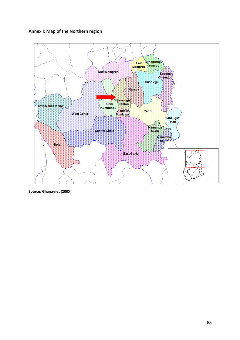
68

Annex I: Map of the Northern region

Source: Ghana-net (200X)

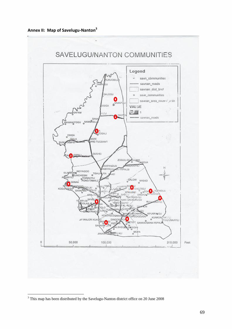
69

Annex II: Map of Savelugu-Nanton3

3 This map has been distributed by the Savelugu-Nanton district office on 20 June 2008

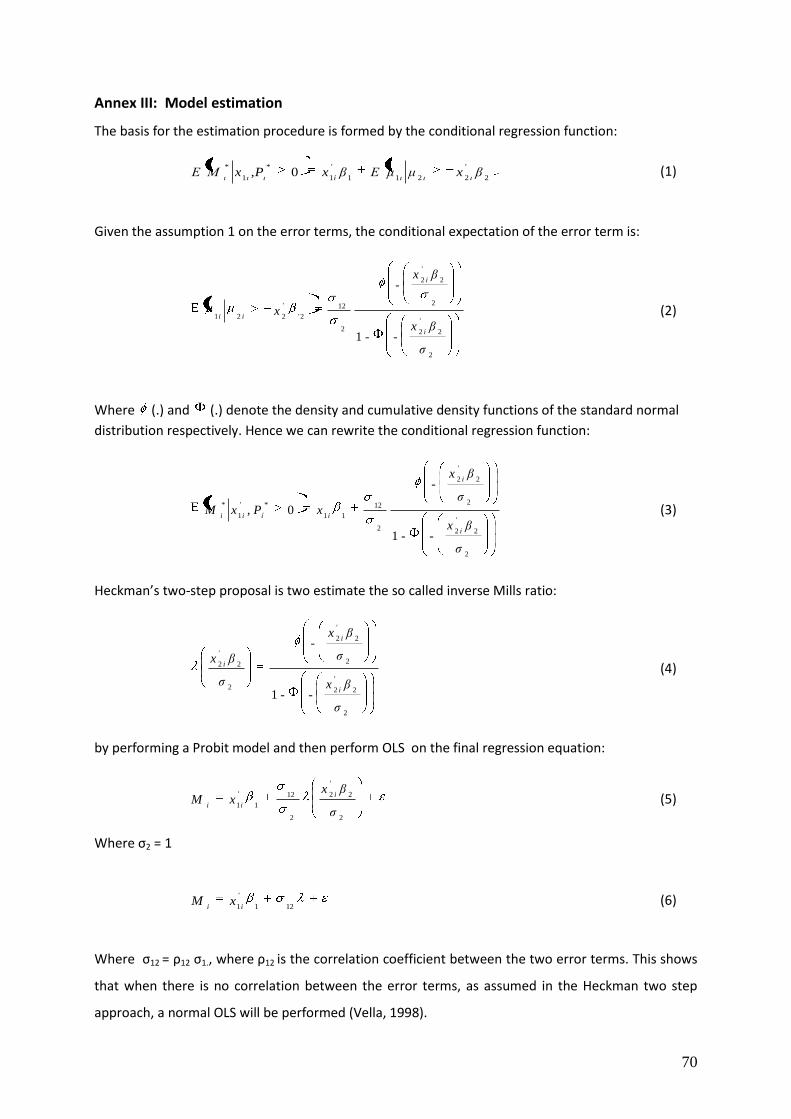
70

Annex III: Model estimation

The basis for the estimation procedure is formed by the conditional regression function:

22211

'

11

*0 βxμμΕβx,PxΜΕ

'

ιιιi

*

ιιι (1)

Given the assumption 1 on the error terms, the conditional expectation of the error term is:

2

2

'

2

2

2

'

2

2

12

2'

'

221

--1

-

σ

βx

βx

x

i

i

ii (2)

Where (.) and (.) denote the density and cumulative density functions of the standard normal

distribution respectively. Hence we can rewrite the conditional regression function:

2

2

'

2

2

2

'

2

2

12

11

*'

1

*

--1

-

0,

σ

βx

σ

βx

xPxM

i

i

iíii (3)

Heckman’s two-step proposal is two estimate the so called inverse Mills ratio:

2

22

2

22

2

22

--1

-

σ

βx

σ

βx

σ

βx

'

i

'

i

'

i (4)

by performing a Probit model and then perform OLS on the final regression equation:

2

2

'

2

2

12

1

'

1σ

βxxM

i

ii (5)

Where ς2 = 1

121

'

1iixM (6)

Where ς12 = ρ12 ς1., where ρ12 is the correlation coefficient between the two error terms. This shows

that when there is no correlation between the error terms, as assumed in the Heckman two step

approach, a normal OLS will be performed (Vella, 1998).

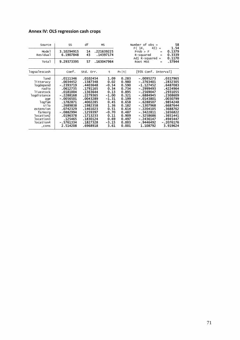
71

Annex IV: OLS regression cash crops

_cons 2.514208 .6968918 3.61 0.001 1.108792 3.919624 location4 -.5761334 .1827328 -3.15 0.003 -.9446492 -.2076176 location3 .125465 .1830124 0.69 0.497 -.2436147 .4945447 location2 .0196378 .1713233 0.11 0.909 -.3258686 .3651441 farmorg -.0882994 .1259397 -0.70 0.487 -.3422811 .1656822 extension .0742329 .1461023 0.51 0.614 -.2204105 .3688762 silo .2689838 .1982358 1.36 0.182 -.1307968 .6687644 logfam .1782871 .4002285 0.45 0.658 -.6288507 .9854248 age -.0056501 .0043289 -1.31 0.199 -.0143801 .0030799 logdistance -.2288168 .2279365 -1.00 0.321 -.6884945 .2308609 livestock .0181004 .1363644 0.13 0.895 -.2569047 .2931055 radio .0612735 .1791165 0.34 0.734 -.2999493 .4224964 logdepend -.2393719 .4403648 -0.54 0.590 -1.127452 .6487083 litteracy .0034452 .1387348 0.02 0.980 -.2763401 .2832305 land .0111346 .0102454 1.09 0.283 -.0095273 .0317965 logsalescash Coef. Std. Err. t P>|t| [95% Conf. Interval]

Total 9.29373395 57 .163047964 Root MSE = .37944 Adj R-squared = 0.1170 Residual 6.1907848 43 .14397174 R-squared = 0.3339 Model 3.10294915 14 .221639225 Prob > F = 0.1379 F( 14, 43) = 1.54 Source SS df MS Number of obs = 58

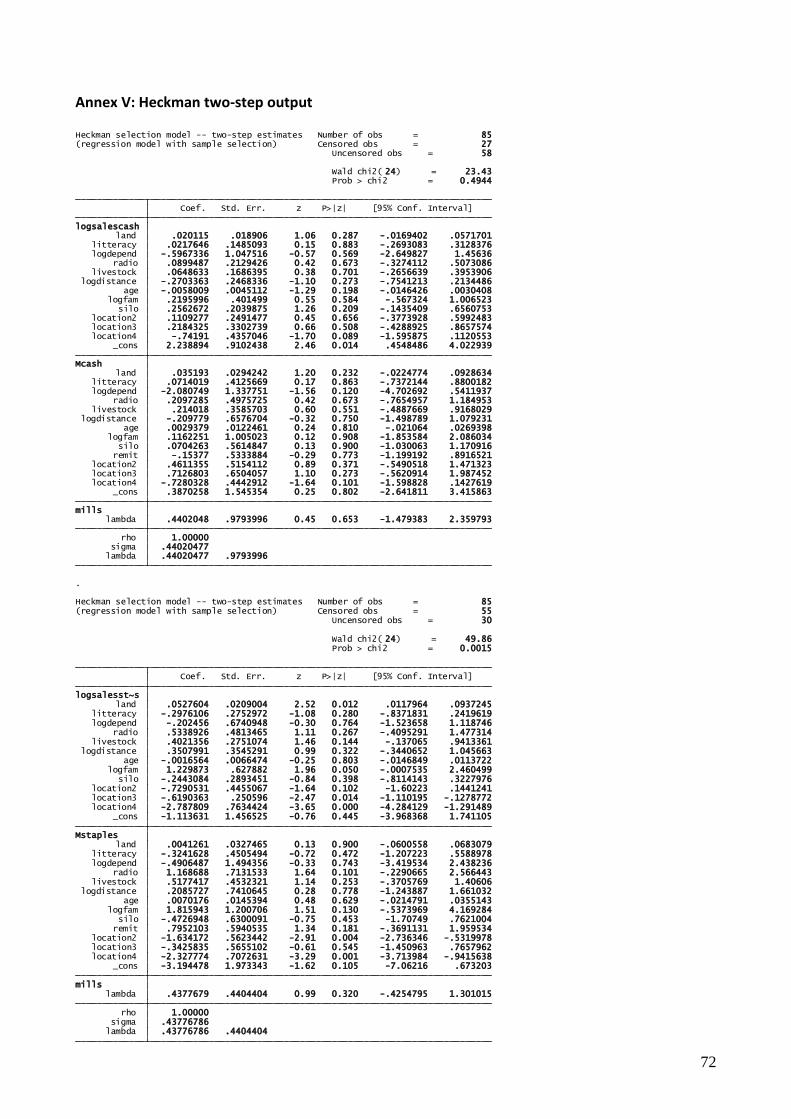
72

Annex V: Heckman two-step output

.

lambda .44020477 .9793996 sigma .44020477 rho 1.00000 lambda .4402048 .9793996 0.45 0.653 -1.479383 2.359793mills _cons .3870258 1.545354 0.25 0.802 -2.641811 3.415863 location4 -.7280328 .4442912 -1.64 0.101 -1.598828 .1427619 location3 .7126803 .6504057 1.10 0.273 -.5620914 1.987452 location2 .4611355 .5154112 0.89 0.371 -.5490518 1.471323 remit -.15377 .5333884 -0.29 0.773 -1.199192 .8916521 silo .0704263 .5614847 0.13 0.900 -1.030063 1.170916 logfam .1162251 1.005023 0.12 0.908 -1.853584 2.086034 age .0029379 .0122461 0.24 0.810 -.021064 .0269398 logdistance -.209779 .6576704 -0.32 0.750 -1.498789 1.079231 livestock .214018 .3585703 0.60 0.551 -.4887669 .9168029 radio .2097285 .4975725 0.42 0.673 -.7654957 1.184953 logdepend -2.080749 1.337751 -1.56 0.120 -4.702692 .5411937 litteracy .0714019 .4125669 0.17 0.863 -.7372144 .8800182 land .035193 .0294242 1.20 0.232 -.0224774 .0928634Mcash _cons 2.238894 .9102438 2.46 0.014 .4548486 4.022939 location4 -.74191 .4357046 -1.70 0.089 -1.595875 .1120553 location3 .2184325 .3302739 0.66 0.508 -.4288925 .8657574 location2 .1109277 .2491477 0.45 0.656 -.3773928 .5992483 silo .2562672 .2039875 1.26 0.209 -.1435409 .6560753 logfam .2195996 .401499 0.55 0.584 -.567324 1.006523 age -.0058009 .0045112 -1.29 0.198 -.0146426 .0030408 logdistance -.2703363 .2468336 -1.10 0.273 -.7541213 .2134486 livestock .0648633 .1686395 0.38 0.701 -.2656639 .3953906 radio .0899487 .2129426 0.42 0.673 -.3274112 .5073086 logdepend -.5967336 1.047516 -0.57 0.569 -2.649827 1.45636 litteracy .0217646 .1485093 0.15 0.883 -.2693083 .3128376 land .020115 .018906 1.06 0.287 -.0169402 .0571701logsalescash Coef. Std. Err. z P>|z| [95% Conf. Interval]

Prob > chi2 = 0.4944 Wald chi2( 24) = 23.43

Uncensored obs = 58(regression model with sample selection) Censored obs = 27Heckman selection model -- two-step estimates Number of obs = 85

lambda .43776786 .4404404 sigma .43776786 rho 1.00000 lambda .4377679 .4404404 0.99 0.320 -.4254795 1.301015mills _cons -3.194478 1.973343 -1.62 0.105 -7.06216 .673203 location4 -2.327774 .7072631 -3.29 0.001 -3.713984 -.9415638 location3 -.3425835 .5655102 -0.61 0.545 -1.450963 .7657962 location2 -1.634172 .5623442 -2.91 0.004 -2.736346 -.5319978 remit .7952103 .5940535 1.34 0.181 -.3691131 1.959534 silo -.4726948 .6300091 -0.75 0.453 -1.70749 .7621004 logfam 1.815943 1.200706 1.51 0.130 -.5373969 4.169284 age .0070176 .0145394 0.48 0.629 -.0214791 .0355143 logdistance .2085727 .7410645 0.28 0.778 -1.243887 1.661032 livestock .5177417 .4532321 1.14 0.253 -.3705769 1.40606 radio 1.168688 .7131533 1.64 0.101 -.2290665 2.566443 logdepend -.4906487 1.494356 -0.33 0.743 -3.419534 2.438236 litteracy -.3241628 .4505494 -0.72 0.472 -1.207223 .5588978 land .0041261 .0327465 0.13 0.900 -.0600558 .0683079Mstaples _cons -1.113631 1.456525 -0.76 0.445 -3.968368 1.741105 location4 -2.787809 .7634424 -3.65 0.000 -4.284129 -1.291489 location3 -.6190363 .250596 -2.47 0.014 -1.110195 -.1278772 location2 -.7290531 .4455067 -1.64 0.102 -1.60223 .1441241 silo -.2443084 .2893451 -0.84 0.398 -.8114143 .3227976 logfam 1.229873 .627882 1.96 0.050 -.0007535 2.460499 age -.0016564 .0066474 -0.25 0.803 -.0146849 .0113722 logdistance .3507991 .3545291 0.99 0.322 -.3440652 1.045663 livestock .4021356 .2751074 1.46 0.144 -.137065 .9413361 radio .5338926 .4813465 1.11 0.267 -.4095291 1.477314 logdepend -.202456 .6740948 -0.30 0.764 -1.523658 1.118746 litteracy -.2976106 .2752972 -1.08 0.280 -.8371831 .2419619 land .0527604 .0209004 2.52 0.012 .0117964 .0937245logsalesst~s Coef. Std. Err. z P>|z| [95% Conf. Interval]

Prob > chi2 = 0.0015 Wald chi2( 24) = 49.86

Uncensored obs = 30(regression model with sample selection) Censored obs = 55Heckman selection model -- two-step estimates Number of obs = 85

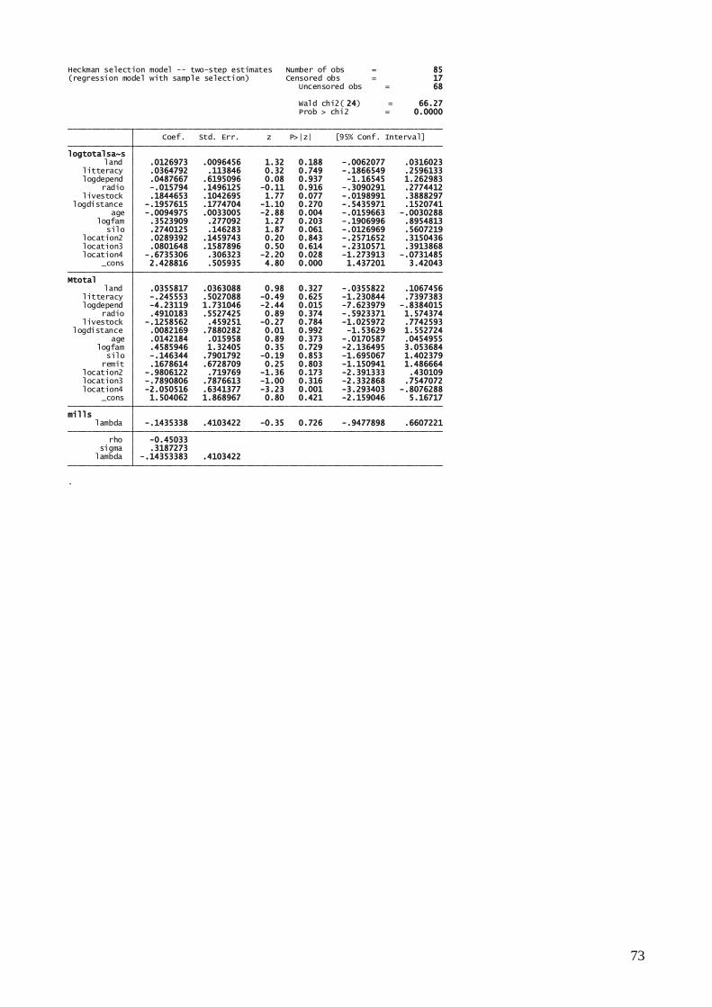
73

.

lambda -.14353383 .4103422 sigma .3187273 rho -0.45033 lambda -.1435338 .4103422 -0.35 0.726 -.9477898 .6607221mills _cons 1.504062 1.868967 0.80 0.421 -2.159046 5.16717 location4 -2.050516 .6341377 -3.23 0.001 -3.293403 -.8076288 location3 -.7890806 .7876613 -1.00 0.316 -2.332868 .7547072 location2 -.9806122 .719769 -1.36 0.173 -2.391333 .430109 remit .1678614 .6728709 0.25 0.803 -1.150941 1.486664 silo -.146344 .7901792 -0.19 0.853 -1.695067 1.402379 logfam .4585946 1.32405 0.35 0.729 -2.136495 3.053684 age .0142184 .015958 0.89 0.373 -.0170587 .0454955 logdistance .0082169 .7880282 0.01 0.992 -1.53629 1.552724 livestock -.1258562 .459251 -0.27 0.784 -1.025972 .7742593 radio .4910183 .5527425 0.89 0.374 -.5923371 1.574374 logdepend -4.23119 1.731046 -2.44 0.015 -7.623979 -.8384015 litteracy -.245553 .5027088 -0.49 0.625 -1.230844 .7397383 land .0355817 .0363088 0.98 0.327 -.0355822 .1067456Mtotal _cons 2.428816 .505935 4.80 0.000 1.437201 3.42043 location4 -.6735306 .306323 -2.20 0.028 -1.273913 -.0731485 location3 .0801648 .1587896 0.50 0.614 -.2310571 .3913868 location2 .0289392 .1459743 0.20 0.843 -.2571652 .3150436 silo .2740125 .146283 1.87 0.061 -.0126969 .5607219 logfam .3523909 .277092 1.27 0.203 -.1906996 .8954813 age -.0094975 .0033005 -2.88 0.004 -.0159663 -.0030288 logdistance -.1957615 .1774704 -1.10 0.270 -.5435971 .1520741 livestock .1844653 .1042695 1.77 0.077 -.0198991 .3888297 radio -.015794 .1496125 -0.11 0.916 -.3090291 .2774412 logdepend .0487667 .6195096 0.08 0.937 -1.16545 1.262983 litteracy .0364792 .113846 0.32 0.749 -.1866549 .2596133 land .0126973 .0096456 1.32 0.188 -.0062077 .0316023logtotalsa~s Coef. Std. Err. z P>|z| [95% Conf. Interval]

Prob > chi2 = 0.0000 Wald chi2( 24) = 66.27

Uncensored obs = 68(regression model with sample selection) Censored obs = 17Heckman selection model -- two-step estimates Number of obs = 85