Stochastic Anal. Appl. Vol. 20, No. 5, 2002, (1027-1082)

Research Report No. 402, 1998, Dept. Theoret. Statist. Aarhus

Market Forces and Dynamic Asset Pricing

G. PESKIR* and J. SHORISH

**

We study a dynamic model of asset pricing which is driven by two characteristic

market features: the law of investor demand (e.g. ’buy low, sell high’) and the law

of the market institution (which codifies the trading rules under which the market

operates). We demonstrate in a simple investor-specialist trading market that these

features are sufficient to guarantee an equilibrium where investors’ trading strategies

and the specialist’s rule of price adjustments are best responses to each other. The

drift term appearing in the resulting equation of the asset price process may be

interpreted using Newtonian mechanics as the acceleration of a ’market force’. If

either of the market participants is risk-neutral, the result leads to risk-neutral asset

pricing (e.g. the Black and Scholes option pricing formula).

1. Introduction ......................................................................................... 1

2. Description of the model .................................................................... 4

3. Brownian motion and Newtonian mechanics ................................... 11

4. Market force and the specialist’s optimisation revisited ................. 16

5. Solution of the investor’s problem ................................................... 20

6. Solution of the specialist’s problem ................................................. 28

7. Concluding remarks and open questions ......................................... 40

Figures .............................................................................................. 42

References ......................................................................................... 47

1. Introduction

The assumption that the price of a tradable asset follows a stochastic process has its foundations

at least as far back as Bachelier (1900), when it was supposed that asset prices follow a Wiener

process. This supposition has grown in complexity and depth over time in both Economics and

Finance, aided by the martingale property of Brownian motion, and especially by the development

of the Ito calculus. The ability to derive properties for functions of stochastic processes has led

to tremendous work on the pricing of derivative securities, perhaps the best known being the

Black and Scholes (1973) option pricing formula. This research initially took the price process as

exogenously given—it was assumed that prices would simply follow one or another (usually quite

tractable) stochastic process. The primary purpose of asset prices, i.e. to clear the asset market,

was often ignored.

* Centre for Mathematical Physics and Stochastics (supported by the Danish National Research Foundation).* Centre for Analytical Finance (supported by the Danish Social Science Research Council).

** The author gratefully acknowledges support from the Centre for Non-Linear Modelling in Economics (supported by the Danish Social ScienceResearch Council, and the Research Foundation of the University of Aarhus).Mathematics Subject Classification 2000. Primary 91B24, 91B28, 91B50, 93E20. Secondary 91A15, 60G51, 60J60, 60J65.JEL Classification Numbers C60, G12, G13.Key words and phrases: Market microstructure, asset pricing, market force, inertial frame of reference, accelerated frame of reference,(geometric) Brownian motion, Newtonian mechanics, Smoluchowski’s approximation, optimal stochastic control, the Hamilton-Jacobi-Bellmanequation, Markov property, Ornstein-Uhlenbeck process, Levy process. goran@imf.au.dk

1

More recently, researchers have investigated under what conditions asset prices may both fulfil

their market-clearing function as equilibrium prices (so that in equilibrium what is supplied suffices

to cover what is demanded), and at the same time be realized as a stochastic process (see e.g. Breeden

1979, Duffie and Zame 1989, Duffie 1996). Such models usually place the stochastic structure upon

an exogenous information process (e.g. arrival of news, dividends, etc.) and then find prices as the

equilibrium of a market with optimizing agents. Prices inherit some, although usually not all, of the

properties of the exogenous stochastic process—they are in a sense derivatives of the underlying

randomness. The key word here is inherit, as it is most often the case that (expected) prices are

taken as given by the market participants. In addition, the market institutions themselves may be

ignored for the sake of exposition: a notable example of this is the assumption that there exists a

’continuum’ of market makers, so that the imperfect competition between them in fact reduces to

the perfectly competitive outcome via Bertrand competition.

By contrast, we attempt in this paper to show that the market institutions may be included by

specifying a pricing rule for those who set the price (e.g. market maker, specialist, etc.). This pricing

rule embodies the allowable behavior that the market participants are allowed to undertake, and may

include incentives on the part of the market’s employees to promote trade, reduce volatility, etc. It

is these employees who are assumed to have, literally, market making power: they set the prices

which the market may follow, in order to clear the market. Note that in this setting we still wish

to involve an underlying stochastic process—however, the mechanism by which this randomness

is transmitted to the market participants is now identified with the pricing rule.

In this paper we introduce a technique for analyzing the relative impacts of the market

participants and the underlying randomness upon the equilibrium asset price. This technique is

intimately related to the structure of stochastic processes in general and is the first to exploit (to

the best of our knowledge) a remarkable property of those Levy processes which are commonly

found in most models of randomness in financial economics. Under these circumstances we are

able to identify a naturally occurring partition of the dynamics which describe the equilibrium of

the model. On the one hand there exists an ’inertial frame’, given by the fundamental price (Lucas

1987), which is in a sense the outcome of the model without the active participation of the agents.

Overlaid upon this is the ’accelerated frame’ which clearly exposes the equilibrium byplay between

a buyer and a seller of the asset. It is this byplay which can be identified with a ’market force’,

and which is purely external to the ’natural’ determinants of the asset price.

The model is a simple specialist-investor trading model. The underlying ’fundamental’ system

contains only a stochastic process for an asset’s dividend (which may be estimated from the observed

values), and a risk-free bond process. The dividend process induces, in the inertial frame, the

fundamental (or no-arbitrage) stock price, which although random does nothing except remain in

this basic state. This captures the notion that without market participants, the underlying randomness

will have no external effects (’forces’) upon it. Although not truly existing in its own right, the

fundamental price has important implications as a benchmark in the specialist’s pricing rule.

We assume that the specialist must obey the rules of the market institution—this limits how

she can affect the asset price process, and also induces a preference ordering over the volume of

trade (so that the specialist prefers more volume to less volume). We suppose that these rules allow

the specialist to adjust the level of relative changes in the asset price, which amounts to setting

the conditional expectation of the future price (see Section 2). The specialist chooses this level

2

adjustment to maximize the expected discounted stream of preference-weighted portfolio returns.

Meanwhile, the investor may trade in the asset, invest in bonds, or both. If he trades in the asset

he trades only with the specialist. The investor chooses his portfolio weights in order to maximize

utility subject to a wealth constraint.

The trading interaction between the specialist and the investor imposes ’market forces’ upon

the stochastic process of the asset price—these market forces are derived in rigorous fashion using

1) the law of demand which the investor obeys (’buy low, sell high’), and 2) the market rules

which dictate allowable specialist behavior, and fix the specialist’s preferences for trading volume.

The market forces are defined in the same way as conservative forces are defined in Newtonian

mechanics. In fact, one may easily define all 3 of Newton’s Laws of Mechanics within this economic

context. We demonstrate that in the dynamic (’accelerated’) system there exists an equilibrium in

which the optimal action of the specialist is akin to the ’acceleration’ of a market force which the

specialist induces. This is an application of Newton’s Second Law, which defines a net force as

proportional to an acceleration of a body. In addition, Newton’s First Law states that in the absence

of market forces the system will obey the fundamental (’inertial’) system dynamics—prices will

follow the fundamental process.

Perhaps most interesting is the analogue of Newton’s Third Law, that there is a balance of forces

in equilibrium. We show that the balancing force to the specialist’s optimal action is a function

of the investor’s risk preferences. The strength of the balanced forces, and hence the behavior

of the time path of the asset price, may be measured in a well-defined way using the investor’s

attitude towards risk. Standard comparative statics techniques may be used to determine the change

in market forces with respect to a change in the investor’s risk preference. This underscores the

advantage of the physical system analogy, as the mapping between investor risk and the resulting

asset price process is quite straightforward, being given by the Second Law’s definition of the

market force and by the Third Law’s balance of forces.

The structure of the paper is as follows. Section 2 presents the model, in which the various

fundamental and dynamic system characteristics are defined. Section 3 presents an historical

perspective on Newtonian mechanics and the interpretation of the solution of the model as a

physical ’market force’. Section 4 introduces a formal definition of the market force and clarifies

the specialist’s problem using the terminology and techniques of Section 3. Sections 5 and 6

present the solutions to the investor’s problem and the specialist’s problem, respectively. They

demonstrate the existence of market forces and their relation to the investor’s risk preferences.

Section 7 concludes and provides an agenda for future research.

3

2. Description of the Model

In this section we introduce the model and its basic assumptions, and explain their mathematical

and economic relevance.

The idea that a market price fluctuates around a ’fundamental’ value is classic, and the extent

to which stock prices would tend to revert to their mean values over long time horisons has been

the subject of long-standing attention in the finance literature. For example, the popular model of

Black and Scholes (1973) suggests that the stock price St follows a geometric Brownian motion:

(2.1) dSt = St

��dt + �dWt

�where the drift rate �2 IR and volatility �> 0 are assumed constant, and W = (Wt)t�0 is a

standard Wiener process1. To overcome disagreements of this assumption with observation, much

attention has been given in (2.1) to generalising both the �-term (leading to stochastic volatility

models) and the dWt-term (leading to Levy process models). Less attention, however, has been

given to the form of the �-term, and this is one of the foci of the present work.

More specifically, and in view of the mean-reversion puzzle stated above, we focus on the

dynamical aspect of this question: What is � to be, where does it originate, and how is it

determined? It should be emphasised that although for simplicity we leave the volatility � constant,

and the noise term equal to dWt , a more realistic picture will be obtained if � is allowed to

be random, and dWt is replaced by dLt where (Lt)t�0 is a Levy process2. We do not want

the technical complexity of these more general assumptions to obscure the clarity of the dynamical

issue we concentrate upon. [It seems more likely, moreover, that these two quantities are to be

determined by statistical observations of the real-world stock price3 (cf. Barndorff-Nielsen 1998).]

If it turns out that the asset price can be modeled by a well-defined stochastic process, then it

seems reasonable to look back at the origins of physical models of this type (e.g. Brownian motion)

and their exact derivations and interpretations. We present a quick overview of this development

in the next section. (We want to stress that the reader must be familiar with these results in order

to understand the basic hypotheses of the model below at a more satisfactory level.)

Our main aim in this study is to describe dynamical aspects of the stock price movement and

initiate a theory which is aimed at uniting its kinematics4 and dynamics, and which is built upon

analogies with the laws of classical mechanics. The central new concept which arises in this attempt

is the concept of the market force. [We would like to point out, however, that the theory presented

below is an idealisation of the real world phenomena. Only after the effects of more general �and Lt are incorporated will the entire picture be more realistic and satisfactory.]

1. The Model Setup. We consider a model of asset pricing which is driven by two characteristic

market features: (i) the law of investor demand (e.g. ’buy low, sell high’) and (ii) the law of the

1 We assume that all stochastic processes and variables appearing throughout are defined on a given and fixed probability space (;F ; P ) .The symbol (Wt)t�0 is used throughout to denote a standard Wiener process, which we also call a standard Brownian motion withoutmaking any difference between these two processes (see Section 3).

2 A stochastic process (Lt)t�0 with right-continuous sample paths (having also left-limits) is called a Levy process if it has stationaryindependent increments, i.e. for every choice of times 0� t0<t1<t2 . . . the increments Lt0 , Lt1�Lt0 , Lt2�Lt1 . . . form a sequenceof independent random variables which moreover are identically distributed whenever t0 = t1 � t0 = t2 � t1 = . . . . These processesare time-homogeneous Markov processes and may have jumps (the only Levy process without jumps is a Brownian motion with drift.) It isknown that these processes can well capture key stylized features of the observed stock price, for more information see Shiryaev (1999).

3 Through its dividends, for instance, as suggested below.4 While kinematics purely describes motion without giving attention to its cause, the primary objective of dynamics is to describe its cause.

4

market institution (which codifies the trading rules under which the market operates). Thus, the

market participants are: (i) an investor (who can be also seen as a representative investor, i.e.

an aggregate of ’small’ investors) and (ii) a specialist (who can be identified with the trading

mechanism of the market institution). There exists a risky asset (or stock) and the investor is

assumed to has at his disposal a risk-free asset (or bond). The bond continuously compounds at

a constant interest rate r > 0 .

The dividend Dt paid by the stock is assumed to evolve1 according to:

(2.2) dDt = �Dt dWt

where � > 0 (volatility) and (Wt)t�0 is standard Brownian motion (a source of randomness)2.

The fundamental stock price is then defined3 to be the expected value4 of all future dividends:

(2.3) Sot = E

�Z 1

te�r(s�t)Ds ds

�� FWt

�where FW

t = �(fWs j 0� s� tg) is the information set available5 at time t .

The strong solution of (2.2) satisfying D0 = d> 0 is given by

(2.4) Dt = d exp

��Wt � �2

2t

�.

This process is a martingale relative to the natural filtration FDt = �(fDs j 0� s� tg) which

coincides with FWt . Observe also that Dt ! 0 as t ! 1 , although E(Dt) = d for all t .

By the martingale property and Fubini’s theorem we find:

(2.5) Sot =

Z 1

te�r(s�t) E(Ds j FW

t ) ds = Dt

Z 1

te�r(s�t) ds

=Dt

r= s exp

��Wt � �2

2t

�where s = d=r and So0 = s .

In deciding how to revise the stock price, the specialist faces constraints specified by the

market institution (see e.g. Ait-Sahalia 1998, Madhavan and Smidt 1993). It will be assumed that

the specialist adjusts the stock price through relative returns according to the following rule:

(2.6)dStSt

= �tdt +dSotSot

where dSt=St is the relative return of the market price, dSot =Sot is the relative return of the

1 All stochastic integrals appearing throughout are understood in Ito’s sense.2 By selecting a different dividend process (which is to be done in accordance with observations of dividend streams of each specific stock) one

will obtain a more realistic picture of real-world stock prices as stated following (2.1) above.3 As in Lucas (1978).4 Given a random variable X and a �-algebra G , by E(X j G) we denote the conditional expectation of X given G . We interpret it as

the best estimate of X on the basis of our knowledge of G .5 Given a stochastic process (ft)t�0 by �(f fs j 0� s� t g) we denote the smallest �-algebra on generated by fs for 0� s� t .

Speaking informally, this �-algebra contains all information about the path of the process until time t , and vice versa, knowing all about thepath of the process until time t , we also know the �-algebra.

5

fundamental price, and �t is the drift chosen by the specialist. Thus, the specialist ’controls’

the market price through the choice of �t . For simplicity, we shall deal with Markov controls

�t = �(t; St) , but other treatments may also be of interest (deterministic or open loop controls

�t = �(t) , feedback or closed loop controls �t being �(fSs j0�s� tg)-measurable, and others).

In view of (2.3) or (2.5) we see that a more complete notation for the stock price St in (2.6)

would be S�t , but we shall often omit � for simplicity.

We note in (2.6) that �t � 0 if and only if (St)t�0 = (Sot )t�0 if and only if there is no control

exercised by the specialist, and if and only if there is no ’external’ force (influence) exerted. In

this case the price is said to be in a ’fundamental equilibrium’. (See next section and in particular

Subsection 3.4 below for a full explanation of these words and concepts.) Observe that the same

equivalence holds in the case when �t is not always 0 , but only becomes 0 from a time t0until a time t1 . Then St will be equal to So

t + c for all t0 � t � t1 where c = St0�Sot0 . The

remaining statements from the equivalence relation above extend to this case in an obvious manner.

These facts will reveal some analogy with Newton’s first law of motion (see the next section).

From (2.5) we see that Sot solves:

(2.7) dSot = �So

t dWt

so that (2.6) in the case of a Markov control �t = �(t; St) can be rewritten as1:

(2.8) dSt = St��(t; St)dt + �dWt

�where � = �(t; s) is a deterministic function belonging to an admissible2 class of actions taken

by the specialist. The specialist’s aim is to determine an optimal �� = ��(t; s) from this class.

If we now consider the log-price:

(2.9) Xt = log�St�

it follows by Ito’s formula that Xt solves:

(2.10) dXt = b�(t; Xt)dt + �dWt

where b�(t; x) = �(t; ex)��2=2 , and this holds for any admissible � = �(t; s) . Thus, by

Smoluchowski’s argument reviewed in the next section, once the optimal ��=��(t; s) is found,

we may think of it as the acceleration of the market force being exerted as a superposition of

external influences by the market players. Thus, formally we can write:

(2.11) ��(t; s) � the acceleration of the market force.

These considerations will be clarified in Sections 4 and 5 below.

2. The Specialist’s Optimisation. How does the specialist determine the optimal adjustment �t ?

We suppose that given a demand function Nt as the number of shares of the stock required by

1 Observe that the model is arbitrage-free and complete, i.e. there exists a unique equivalent martingale measure, see e.g. Shiryaev (1999).2 The word ’admissible’ refers throughout to a condition or a set of conditions which ensure that all objects under considerations are ’well-

defined’ and ’well-behaved’. It also means that these conditions are not restrictive and can be made precise by means of standard mathematicaltechniques, but for the elegance of the exposition such a description is omitted.

6

an investor, by the rule of the market institution the specialist must take the opposite side of the

trade (see e.g. Ait-Sahalia 1998), i.e. she must clear the market and hold �Nt shares of the stock.

We note in passing that this rule is connected with Newton’s third law of motion (see the next

section). In order to formulate the specialist’s criteria for selecting an optimal �t , we identify the

instantaneous excess return provided by the stock (without discounting) with:

(2.12) dRt = Dtdt + dSt .

Without loss of generality we shall neglect the dividend term Dtdt in (2.12) in what follows.

Depending upon the choice of discounting1 (which will be analysed in Subsection 4.2 below),

we shall study two possible formulations of the specialist’s optimisation problem. The formulations

imply markedly different consequences for the asset price process. Setting:

(2.13) eSt = e�rtSt

the first specialist’s formulation is to solve:

(2.14) sup�

E

�Z 1

t(�N�

s ) deSs �� Ft

�where Ft represents the information set available at time t , and N�

s is an optimal investor’s

demand at time s given the stock price (to be specified below).

The second specialist’s formulation is to solve:

(2.15) sup�

E

�Z 1

te�rs(�N�

s ) dSs�� Ft

�with Ft and N�

s as above. Thus, in this case the discounting is applied before the d-sign and

not after as above (see Subsection 4.2 below for a complete argument).

In both formulations the supremum is taken over all �= (�s)s�t from an admissible class

for which (2.6) makes sense; in this paper we shall study Markov controls �t = �(t; St) , but

other controls may also be of interest (indeed, the case of constant � will already give a good

insight into the more general problem). The �-algebra Ft is naturally assumed to be equal to

FtS;Z = �(fSs; Zs j0�s� tg) , where Ss=S�s is the stock price at market, and Zs is investor’s

wealth (to be specified below). It should be observed that the existence of a strong solution of (2.8)

implies that the �-algebra FtS coincides with Ft

W and thus FtS;Z = Ft

W as well.

We shall see later that the crucial role in the treatment of the specialist’s problems (2.14) and

(2.15) is played by the Markovian structure2 of the process (St; Zt) (or just the process St in

the case of constant � ). This will enable us to reformulate problems (2.14) and (2.15) as optimal

stochastic control problems which can then be solved explicitly. We shall continue our treatment

of these problems in Section 6 below.

1 We address this discounting question because it is of a fundamental nature often overlooked in current research, i.e. the distinction betweencontinuous ’modeling’ time and ’calendar’ time during which certain actions may not be available to the market participants.

2 A Markov property states that the best estimate of the future given the entire past coincides with the best estimate of the future given onlythe present. In other words, if we wish to predict a future behaviour of a Markov process, then our knowledge of its entire past is irrelevantand only its present state is what matters. We also say that the process starts ’afresh’ at each instant of time. More analytically, the Markovproperty of the process (Xt)t�0 can be expressed by requiring that Ex(Y � �t j FX

t ) = EXt (Y ) , where X starts at x under Px ,and �t is a shift operator satisfying Xs � �t = Xs+t . In this identity it is important to realise that Y may be any measurable functionof the entire path fXt j t � 0g of the process, e.g. we may take Y = 1

0 f(t;Xt) dt with some f=f(t; x) as used often throughout.

7

3. The Investor’s Optimisation. To formulate the investor’s problem assume that his initial wealth

is z>0 , and that he is free to transfer his holdings continuously in time from one investment to

another without paying transaction costs. There is no restriction on borrowing or lending, and short

sales are allowed. We assume that the investor has at his disposal two investment possibilities: the

stock given by (2.6) above, and the risk-free bond satisfying:

(2.16) dBt = rBt dt

with B0 = 1 . Thus Bt = ert continuously compounds at the constant interest rate r>0 .

The fraction of investor’s wealth held at time t in the stock is conveniently denoted by

(2.17) ut =Yt

Xt + Yt

where Yt is the wealth held in the stock (may be positive or negative), and Zt := Xt + Yt is the

total wealth held both in the stock and the bond. Thus Xt is the wealth held in the bond, and

while Xt may be also positive or negative, we shall see that the transversality condition imposed

later on will ensure that Zt � 0 for all t .

It is easily verified that: (i) ut < 0 corresponds to short sales of the stock; (ii) ut > 1corresponds to borrowing from the bank; and (iii) ut 2 [0; 1] corresponds to a long position in

both the stock and the bond.

Given a consumption rate ct , the investor’s wealth process Z=(Zt)t�0 is assumed to satisfy

to following budget equation:

(2.18) dZt = (1�ut) rZt dt + utZt

��tdt + �dWt

� � ctdt

where (1�ut)rZt dt is the fraction of wealth held in the bond, utZt

��tdt+�dWt

�is the fraction

of wealth held in the stock, and ctdt is the fraction of wealth consumed. By writing (2.18) in

this form we are actually imposing a self-financing property on the strategy of the investor. (This

will be addressed in more detail in Section 4 below.)

If the specialist is applying Markov controls of the form �t = �(t; St) which lead to the

stock price (2.8), then from (2.18) we see that our basic Markov process is (St; Zt) , which is two-

dimensional. This is not the case when �t is constant; in this case Zt is a one-dimensional Markov

process. This remark will be of interest in the following analytic treatment of the investor’s problem.

In the sequel we will avoid dealing with the time of bankruptcy:

(2.19) � = inf f t > 0 j Zt = 0 g

and replace it with a transversality condition (specified later) which will imply that at the ’end of

time’ the wealth must be non-negative (i.e. the investor cannot ’die’ holding a debt).

Given a utility function U = U(c) , the investor’s aim is to solve:

(2.20) supu;c

E

�Z 1

te��sU(cs) ds

�� Ft

�where Ft equals Ft

Z or FtS;Z depending on whether �t is a function of St or not,

8

respectively. In any case, the �-algebra Ft is always contained in FWt . The rate of time

preference � is strictly positive, and will often be assumed equal to r . The supremum in (2.20)

is taken over admissible u=(us)s�t and c=(cs)s�t for which (2.18) makes sense.

The utility function of the investor is assumed to be:

(2.21) U (c) =c �1

(0< < 1)

which has an Arrow-Pratt coefficient of relative risk aversion given by �cU 00 (c)=U

0 (c) = 1� .

We shall also deal with the logarithmic utility function:

(2.22) U0(c) = log(c)

which is obtained as a limit of (2.21) for # 0 . These utility functions will be sufficient to grasp

most of the essentials offered by the model. The problem (2.20) in this case reduces to the problem

posed and solved by Merton (1969; 1971).

To relate the number Nt of shares of the stock held by the investor to the fraction of her wealth

ut appearing in (2.17), recall that the self-financing property (2.18) states (see Section 4 below):

(2.23) Zt = ntBt + NtSt = z +

Z t

0ns dBs +

Z t

0Ns dSs � Ct

where Ct =R t0 csds , or in other words:

(2.24) dZt = ntdBt + NtdSt � dCt

where dCt = ctdt . Using (2.6)+(2.7) and (2.16) we can rewrite (2.24) as:

(2.25) dZt = rntBt dt + NtSt��tdt + �dWt

� � ctdt .

Comparing it with (2.18) above, we see that:

(2.26) nt = (1�ut) ZtBt

& Nt = utZtSt

.

Thus, the model (2.18) based on fractions of wealth ut and (1�ut) is equivalent to the

model (2.23) based on the self-financing property of the portfolio (nt; Nt) . The latter will be

analysed in Section 4 through the passage from a discrete time case to the continuous time case.

The problem (2.20) will be treated analytically in Section 5 below.

4. Concluding Remarks. Thus, if it is known (from the trading rules specified by the market

institution) that the stock price (St) will be driven as in (2.6) for some admissible (�t) ,

then the specialist-investor equilibrium is achieved as follows. The investor takes any admissible

�=(�t) as given and solves her optimisation problem (2.20), thus obtaining an optimal demand

N�(�) = (N�t (�)) which depends on � . Given this demand function the specialist solves her

optimisation problem (2.14) or (2.15) and obtains the optimal drift �� = (��t ) . As the optimal

N�(�) found by the investor applies to any � , it will also apply to the optimal �� , thus leading

to the optimal demand function N�� :=N�(��) . This procedure gives the equilibrium actions

9

(��; N��) which are mutual best responses. In accordance with our considerations taken up in

the next section, and as already stated in (2.11), this solution establishes a ’dynamic equilibrium’

defined by a ’market force’ with ’acceleration’ � ��t . This identification utilizes Newton’s second

law of motion (the principle of ’superposition’ of forces), in which the forces are an ’action force’

of the investor and a ’reaction force’ of the specialist (see the next section for more details).

10

3. Brownian Motion and Newtonian Mechanics

Our aim in this section is to recall a few historical facts which will clarify our conclusions

in the previous and following sections. The term ’Brownian particle’ below refers to a body of a

microscopically visible size suspended in a fluid. Its motion is caused by a molecular bombardment

of the fluid and is called (physical) Brownian motion. The thermal molecular motion of the fluid

is in accordance with the kinetic theory of heat.

1. Brownian Motion. The Einstein-Smoluchowski theory of Brownian motion (1905-1906)

suggests that the position of the particle started at x is described by

(3.1) x + �Wt � N(x; �2t)

where � is a diffusion coefficient (see Einstein 1905, Section 4). Einstein’s argument, although very

successful for many reasons, does not give a dynamical theory of Brownian motion (which would

rely upon Newtonian mechanics). His analysis is solely based upon the hypothesis that the physical

Brownian motion has stationary independent increments, which in turn implies that the transition

probability density p(t; x; y) satisfies the heat equation (also called the forward equation):

(3.2)@p

@t=

�2

2

@2p

@y2

upon assuming implicitly1 that P (jx+�Wtj�") =Rfjx+yj�"g p(t; x; dy) = o(t) as t # 0 .

Langevin (1908) initiated, and Ornstein and Uhlenbeck (1930) developed, a new theory of

Brownian motion which is truly dynamical. This theory is derived from Newton’s second law

F = ma , which in this specific case reads as follows:

(3.3) md2Xt

dt2= �m�Vt + m�

dWt

dt

where Xt is the position of the particle, Vt is its velocity, �m�Vt is a frictional force (due

to the fluid), and m� (dWt=dt) is a fluctuating force (due to the molecular bombardment). It

is known from experiment that frictional forces are proportional to velocities, and Doob (1942)

clarified the specific form of the fluctuating force appearing in (3.3): the velocity Vt for t!1must become Gaussian.

The equation (3.3) is equivalently rewritten as the following system:

(3.4) dXt = Vtdt

(3.5) dVt = ��Vtdt + �dWt .

Upon imposing X0 = x and V0 = v , the (strong) solution of this system is given by

(3.6) Xt = x +1

�

��Wt � Vt + v

�(3.7) Vt = e��tv + �e��t

Z t

0e�rdWr .

1 This is suggested in Nelson (1967). [A more pleasing condition of the sample path continuity can also be used to the same effect.]

11

These processes are Gaussian, and by analysing the covariance structure, the following fact is easily

verified: If � ! 1 and � ! 1 such that b� := �=� remains constant, then:

(3.8) (Xt)t�0��! (x + b�Wt)t�0 .

This relation1 clearly indicates that the ES theory of BM is a limiting case of the OU (i.e. Newtonian)

theory of BM for infinite friction and infinite heat (for more details see Nelson (1967)).

Both theories are in agreement with experiment and to a large extent offer predictions which are

numerically indistinguishable. While the OU theory is in accordance with Newtonian mechanics, the

ES theory is more elegant and computationally more accessible. For example, while ((Xt; Vt))t�0is a (two-dimensional) Markov process, the process (Xt)t�0 itself does not possess the Markov

property. As (Wt)t�0 is both a Markov process and a martingale, the passage from Xt to Wt

may be viewed as a convenient approximation. Recalling the power of Ito’s theory, as well as the

optional sampling argument, one gets a clear picture of why the ES Brownian motion prevailed

in probability theory as a winner. It should be stressed, however, that according to Newtonian

mechanics, the passage from Xt to Wt is only a convenient idealisation.

The matters change dramatically if the Brownian particle is exposed to an external force field:

the ES theory breaks down! (A clear and immediate argument for this statement is obtained by

noting that the property of stationary independent increments gets lost.)

2. Brownian Motion in a Force Field. Suppose that a Brownian particle is under influence of

an external force given by

(3.9) F (t; x) = mA(t; x)

where m is the mass of the particle and A(t; x) is the acceleration at position x at time t .

Then the Langevin equations of the OU theory have the following form:

(3.10) dXt = Vtdt

(3.11) dVt = A(t; Xt) dt � �Vt dt + �dWt

with X0 = x and V0 = v , and where the three terms on the right hand-side represent the external,

frictional, and fluctuating force, respectively. Observe that we can no longer consider the velocity

process by itself—thus the treatment is inherently two-dimensional.

Similarly to the case A � 0 , when an external force is present, there is a one-dimensional

Markov process (discovered by Smoluchowski) which under certain circumstances is a good

approximation of the position process (Xt)t�0 in (3.10). This process is given by

(3.12) dXt =A(t; Xt)

�dt +

�

�dWt .

The following result is established by Nelson (1967): The solutions (Xt)t�0 of (3.10) and (3.12)

for large � and � are close with probability 1 uniformly for t in compact sets of [0;1�.

Thus, in exactly the same way as the ES Brownian motion (3.1) is a convenient approximation

1 This is a convergence in law of stochastic processes. Stronger convergence results can also be established, see Nelson (1967).

12

of the OU Brownian motion (3.4), the solution of (3.12) is a convenient approximation of the OU

Brownian motion (3.10) which is under influence of an external force (3.9). It can be shown that

this approximation is ’good’ if: (i) the time between two observations �t is much larger than

1=� ; and (ii) the external force is ’slowly varying’ (see Nelson (1967) for details).

For these reasons we think of the equation:

(3.13) dXt = �(t; Xt) dt + � dWt

as an idealised description of the position of the particle which is under the influence of two forces:

(3.14) external force � acceleration �(t; x)

(3.15) fluctuating force � Gaussian white noise �(dWt=dt) .

The relevance of this identification1 for our model of asset pricing is given in Subsection 3.4, and

later in Section 4 where the concept of market force is formally introduced. We first recall some

facts from classical physics (see e.g. Weidner and Sells 1965) for convenience and comparison.

3. Newtonian Mechanics. The primary objective of classical mechanics is to describe the causes

of the motions of bodies. Classical mechanics is based upon Newton’s three laws of motion and

has an enormous range of applicability. It successfully describes the motion of objects as small

as molecules (10�9 m) and as large as galaxies (1021 m). Only for the submicroscopic world of

the atom and beyond it, and for speeds approaching the speed of light, must Newton’s laws be

superseded by the more accurate mechanics of the quantum theory and the theory of relativity,

respectively.

Three Newton’s laws of motion are:

(L1) A body subject to no resultant external force moves with a constant velocity:Pi Fi = 0 ) v = const. ;

(L2) If a body is subjected to one or more external forces, the time derivative of the body’s

momentum is equal to the sum of the external forces acting upon it:

d(mv)dt =

Pi Fi ;

(L3) If one body interacts with a second body, the force of the first body upon the second is

equal in magnitude but opposite in direction to the force of the second body upon the first:

F2;1 = �F1;2 .

Newton’s laws are ’true’ because they are consistent with experiment. Let us further recall a few

facts and implications of these laws.

(1) The first law is Galileo’s law of inertia. It defines the concept of an inertial frame as a

reference frame in which an undisturbed body maintains a constant velocity. Such a body is also

said to be in a translational equilibrium. Thus, a body can be in a translational equilibrium only if

the resultant external force acting on it is zero, or in other words, only if there is no net external

1 In the case of a more general Levy process (Lt)t�0 , the Gaussian white noise in (3.15) is to be replaced by a Levy white noise dLt=dt .

13

influence on the body (such external influences may exist but they must balance (cancel) each other

completely). If, however, a body changes its speed or its direction of motion, it has been acted

upon by an ’unbalanced’ external force.

(2) The second law applies only for observers in inertial frames of reference. Provided that

the forces acting upon a body are known, the second law enables us to predict its future position

in complete detail. Kinematics and dynamics are thus united.

The reader unfamiliar with these principles is invited to work out examples of motion for a

harmonic oscillator (spring problems), a pendulum, and falling body problems, as well as many

others which posses the same structure. This list is endless and even continues in full analogy to

other fields (e.g. problems in electric circuitry based upon Kirchhoff’s laws). Common to all these

examples is that the resultant force acting on the body can be expressed as a function of t; x; x0; x00 ,

where x = x(t) is the position of the body at time t . Then Newton’s second law F = mabecomes a second-order differential equation F (t; x; x0; x00) = mx00 , and upon imposing initial

conditions x(0) = x0 and x0(0) = v0 on the position and velocity, respectively, the solution

x = x(t) describes the future motion in full detail.

The second law embodies the principle of superposition for forces. This allows us to replace a

number of forces acting simultaneously on the body by a single resultant force equal to their sum.

(3) Newton’s third law of motion is a consequence of the conservation of momentum law (which

can be verified experimentally) and the definition of force as the time derivative of the momentum.

The conservation of momentum law states that the momentum (p=mv) lost by one body is equal

to the momentum gained by the other, the total momentum of the system remaining constant.

We can now incorporate these general facts from the theories of Brownian motion and

Newtonian mechanics into the model presented in Section 2.

4. Inertial vs. Accelerated Frames of Reference for the Stock Price Movement. The model

developed in the previous section rests upon the existence of a fundamental stock price following a

stochastic process (in our case the log-price is a Brownian motion but it could be any Levy process).

The stochastic motion of the fundamental price may be seen as taking place in an ’inertial frame’ of

reference, influenced only by the arrival of dividends. The external influence comes from the market

players who change the price through the optimal choice of � . More specifically, the specialist and

the investor act optimally to meet their own demands, and as a result the price changes according

to the optimal � . Consequently, one may think of the resulting price movements as taking place

in an ’accelerated frame’ of reference. Note that, although the optimal � is formally chosen by

the specialist, it is a superposition of the activity of both the specialist and the investor. Thus,

the price movement consists of two parts: its ’fundamental’ part (the one in the ’inertial frame’)

and the ’external’ part (the one which is in the ’accelerated frame’ and which is a product of the

market players). Neither � nor dWt (or more generally dLt ) in (2.1) can be influenced more

significantly by either of the market players1. These quantities are specific to each stock and are

largely determined on a global scale which cannot be controlled by an individual—in other words,

they have to be estimated empirically. Thus it follows that market operations are simply a product

1 To some extent one may compare it with a ’bombardment’ of molecules depending on the viscosity and temperature of the media. Thevolatility � is known to be proportional to the temperature (i.e. heat) and reversely proportional to the viscosity. A Levy process is known toconsist of three parts: a constant drift, a constant volatility, and a jump part. These may be explained by the internal properties of the media,i.e. molecules. Their size and number, influencing the intensity and frequency of the kicks as well as their symmetry or asymmetry, impose aLevy motion upon the particle. A change of the volatility is possible only by changing the temperature, i.e. adding or subtracting heat, or bychanging the viscosity, i.e. the media itself. [These changes, however, rests upon the concept of energy.]

14

of external forces of the market players acting upon an underlying system, which would happily

continue undisturbed on its own path if the market participants were absent.

In the context above the concepts of ’fundamental’ and ’dynamic’ equilibria appear as natural

simplifiers of the thought. In the absence of market operations the stock price is in a ’fundamental

equilibrium’. After the market operations are completed in an optimal fashion, the price is set

into a ’dynamic equilibrium’ (of external forces acting upon it). The ’fundamental equilibrium’

corresponds to an ’inertial frame’ of reference, and the ’dynamic equilibrium’ corresponds to an

’accelerated frame’ of reference. It should be kept in mind that these concepts are about stochastic

motions which are driven by fluctuating forces1.

Thus, the ’fundamental’ equilibrium corresponds to the ’perfect world’ of the fundamental

stock price (the expected present value of all future dividends) in which no external force is exerted

(by market players). In ’this world’ the stock price is governed by the ’fluctuating force’ (i.e.

dividends) which may be viewed as a summary of real world uncertainties. In our model this force

is simplified to �dWt , but both stochastic �’s and more general Levy processes (Lt)t�0 can be

taken instead. [Naturally, this choice must be governed by experimental observations of the stock

and its dividends, and is not under direct influence of market players.]

1 The reader should note the great deal of similarities between the dynamics of the stock price movement in the model above and the dynamicsof moving particles according to the theory of classical mechanics reviewed above. It is known that a physical BM is in a ’fundamentalequilibrium’ (which could be equally well replaced by dynamics of any Levy process). Thus, by definition, a stochastic motion is in an ’inertial

frame’ of reference if it has stationary independent increments. However, if a Brownian particle is under the influence of a ’detectable’ externalforce, then this breaks down—the movement of the particle is set into a ’dynamic equilibrium’ (of the resultant external force acting upon it).The free Brownian particle moves because of a molecular bombardment—we call it a fluctuating force—which consists of many infinitesimallysmall impacts (forces) by each molecule on the particle. These impacts are extremely gentle and perfectly symmetric, but nonetheless, sonumerous and chaotic that they cannot balance (cancel) but produce a movement—that’s why the Brownian particle moves after all, although,looking quite formally, there is no external force exerted in a detectable manner (recall that if a rigid body would be under no influence ofexternal forces, according to the first Newton’s law, it wouldn’t move, or it would move with constant velocity). The existence of physicalBM is a consequence of the fine touch between the two worlds of macro and micro. When looking from the scale of the macro world as wedo, we may think of physical BM as being in an inertial frame, although, if looking from the scale closer to the micro world, this attitudemay and does change.

15

4. Market Force and the Specialist’s Optimisation Revisited

1. We will find it convenient in the first part of this section to denote � in (2.8) by b� . Then

by (2.8) and (2.10) we know that the log-price Xt = log(St) satisfies:

(4.1) dXt = b�(t; Xt)dt + b�dWt

where b�(t; x) = �(t; ex)�b�2=2 . Our main aim now is to show how one can detect an external

influence (force) from (4.1) and formally define it as an equivalence class.

To do so first recall the result of Smoluchowski’s approximation (3.12). Assume that the stock

price (the movement of which is now identified with the movement of a physical particle) is under

influence of an external force given by (3.9). Then the Newtonian dynamics of the motion is

described by equations (3.10) and (3.11). Observe that (3.11) can be written as:

(4.2) dVt = � bA(t; Xt) dt � �Vt dt + �b�dWt

where bA(t; Xt)=A(t; x)=� and b�=�=� . If now � !1 , A(t; x)!1 and � !1 such

that bA(t; Xt) and b� remain constant, then the Nelson result quoted above following (3.12) states

that the solution (Xt)t�0 of (3.10) is close to the solution of the equation:

(4.3) dXt = bA(t; Xt)dt + b�dWt

with probability 1 uniformly over t in compact sets of [0;1�. We may conclude that (4.3)

describes a ’frozen’ picture of the extreme situation where the ’friction’, ’external influence’, and

’heat’ increase in such a manner to balance each other in a linear fashion.

A comparison of (4.3) and (4.1) reveals that:

(4.4) A(t; x) � ���t; ex

� � �2

2�

which is equivalently rewritten as:

(4.5) �(t; x) � 1

�A�t; log(x)

�+

�2

2�2.

These equations display in a clearer manner how �(t; s) in (2.8) relates to the influence of an

external force with the acceleration A(t; x) . It should be noted that this identification relies

upon a perturbation of the initial system through its ’genuine’ parameters � and � as well

as A(t; x) itself.

The preceding considerations indicate that a natural definition of the market force in the context

of (2.8) would be to identify it through its acceleration as:

(4.6) F (t; x) � �(t; s)

where s = log(x) . This identification is as close to the ’actual’ truth as desired (from the point

of view of classical mechanics) up to the choice of an affine transformation. This statement can

now be formalised as follows. Introduce an equivalence relation in the class of all admissible

16

� = �(t; s) such that �1 is equivalent to �2 if and only if �1(t; s) = a �2(t; s) + b for

some real constants a and b with a 6= 0 . In this way the class of all admissible functions

� = �(t; s) splits into equivalence classes consisting of those � mutually equivalent, and in an

obvious accordance with Smoluchowski’s approximation via Nelson’s result, we can identify each

such a class with the acceleration of a market force.

Observe that the ’unknown’ b corresponds to a constant velocity (which in the financial

world of our specialist and investor may also be viewed as if coming from an inertial frame of the

fundamental price). By adding a constant to �(t; s) we are actually setting the price movement

in a ’different’ inertial frame, and the ’unknown’ a corresponds to a ’mass’ which cannot be

specified a priori as the stock price is ’massless’.

A nice feature of the mathematical formalism presented above is that, although we identify

the external force with a class of functions � = �(t; s) , each class will typically admit a

natural representative which is easier to work with. By selecting the optimal constants through the

optimisation problems of the specialist and investor, we are actually determining the ’accelerated

frame’ of the stock price as well as the ’mass’ of the price, or in other words, the actual size

of the market force within the equivalence class of admissible functions. (Nelson 1967 offers a

more sophisticated description of kinematics of stochastic motion. Our approach above is primarily

guided by simplicity of the argument.)

2. In the remaining part of this section we shall describe the essentials which lead to the two

formulations (2.14) and (2.15) of the specialist’s optimisation problem.

Assume for now that trading takes place only at discrete times 0;�t; 2�t; . . . and consider a

fixed time interval [t; t + �t�

with t = n�t for some n � 1 . The self-financing property of

the investor’s portfolio in the interval [t; t+�t�

can be expressed by the budget equation:

(4.7) nt��tBt + Nt��tSt = ntBt + NtSt + ct�t

where the left hand side equals the investor’s wealth at the beginning of the interval [t; t+�t�

(this is the amount that the investor gets if she sells her ’old portfolio’ of [t��t; t�

at today’s

price), and the right-hand side consists of the cost of the ’new portfolio’ which has to be bought at

today’s price) plus the amount Ct = ct�t to be consumed during [t; t+�t�

at rate ct .

Denoting �f(t) = f(t)�f(t��t) , we can rewrite (4.7) as follows:

(4.8) Bt�n(t) + St�N(t) + ct�t = 0 .

Adding and subtracting B(t��t)�n(t)+S(t��t)�N(t) , we can further rewrite (4.8) as follows:

(4.9) B(t��t)�n(t) + S(t��t)�N(t) + �n(t)�B(t) + �N(t)�S(t) + ct�t = 0 .

Letting now �t # 0 in (4.9), and interpreting stochastic integrals in Ito’s sense, we get:

(4.10) Btdnt + StdNt + dntdBt + dNtdSt + ctdt = 0 .

On the other hand, letting �t # 0 in (4.7), we see that the investor’s wealth at time t equals:

(4.11) Zt = ntBt + NtSt .

17

Applying Ito’s formula in (4.11), we get:

(4.12) dZt = ntdBt + Btdnt + dntdBt + NtdSt + StdNt + dNtdSt .

Finally, inserting the self-financing condition (4.10) into (4.12), we end up with the wealth equation:

(4.13) dZt = ntdBt + NtdSt � ctdt

which was used in (2.24).

In the preceding derivation no discounting has been applied. The place to apply it is certainly

the budget equation (4.7). Clearly, the right-hand side should be discounted by e�rt , and for the

left-hand side we shall single out two possibilities: (i) discounting by e�rt , and (ii) discounting

by e�r(t��t) . Obviously, the second choice is more favourable to the investor as it implies that

she can protect her portfolio during the time interval [t��t; t�

from devaluation; it is as if ’the

investor bought today’s price yesterday’.

To regard this in an economically plausible fashion, suppose that the investor does not have

available the possibility of investing the portfolio at the bond rate r between [t��t; t�

. This is as

if the investor is protected from opportunity cost devaluation during that time. That is, the ’bank’

which offers the bond rate is only open at discrete points in time, so that the portfolio value cannot

be invested continuously but only during ’opening hours’. This highlights the difference between

’calendar’ time (where opening hours are assumed to exist) and ’modeling’ time in our framework,

and we include both of these specifications because of the different conclusions they generate. The

modeling time framework (the first discounting choice) is the more common framework in Finance.

It does not allow for arbitrage opportunities at any time, and leads to risk-neutral (or fundamental,

or no-trade) pricing when the specialist is risk-neutral (see Section 6.2). The calendar time model,

on the other hand, will allow arbitrage opportunities to exist for very short time intervals, so that

the market exists even when the specialist is risk-neutral (see Section 6.1).

The first choice leads to the first formulation of the specialist’s problem (2.14), and the second

choice of discounting leads to the second formulation (2.15); both are easily derived as follows.

Given any ft denote e�rtft by eft . Then the first choice of discounting applied in (4.7)

leads to the following equation:

(4.7’) nt��teBt + Nt��t

eSt = nteBt + Nt

eSt + ect�t .

Repeating the rest of the derivation above word by word, we end up with the analogue of (4.13):

(4.13’) d eZt = ntd eBt + NtdeSt � ectdt = NtdeSt � ectdtas d eBt = d(1) = 0 . (Observe that this is also easily obtained from (2.23) by Ito’s formula.) On

the other hand, the second choice of discounting applied in (4.7) leads to the following equation:

(4.7”) ent��tBt + eNt��tSt = entBt + eNtSt + ect�t

and in exactly the same way as above, we end up with another analogue of (4.13):

(4.13”) d eZt = entdBt + eNtdSt � ectdt .

18

Clearly, the two equations (4.13’) and (4.13”) are much different.

Observe that in the first case of (4.13’) all the gain NtdeSt comes solely from the stock—this is

intuitively clear since a discounted bond produces no variation. Thus, in this case the existence of

a bond is completely irrelevant and everything can be summed up within the stock. In the second

case of (4.13”), however, a pure stock gain is eNt dSt , and the existence of a bond is relevant as

it can produce a gain of its own (being equal to entdBt ).

Under discounting (i) the investor’s gain in the stock equals Nt deSt . Recalling that the

specialist must take the opposite side of the investor’s trade, we obtain the specialist’s problem

formulated as in (2.14). Similarly, under discounting (ii) the investor’s gain in the stock equalseNt dSt . From this we obtain the specialist’s problem formulated as in (2.15). We shall see later

that these two problems have very different solutions.

19

5. Solution of the Investor’s Problem

Consider the investor’s problem (2.20) under the dynamics of his wealth (2.18). In the treatment

of this problem below it is both suitable and instructive to distinguish cases depending on the

functional form of the drift term �t appearing in (2.18).

1. The case of �t � � . In this case the wealth equation (2.18) reads as follows:

(5.1) dZt =��

(��r)ut+r�Zt � ct

�dt + utZt�dWt

where ut = u(Zt) and ct = c(Zt) for some admissible functions z 7! u(z) and z 7! c(z) � 0for which (5.1) makes sense. The process Z = (Zt)t�0 is a Markov process, and Ft in (2.20)

can be taken FZt . Thus the problem (2.20) reduces to solve:

(5.2) supu;c

Ez

�Z 1te��sU(cs) ds

�:= H(t; z)

where it is natural to impose the following transversality condition:

(5.3) limt!1Ez

�H(t; Zt)

�= 0

with Z0 = z under Pz . By the Markov property the supremum appearing in (2.20) is then equal

to H(t; Z�t ) . Moreover, by applying the Markov property at time t we easily find that:

(5.4) e�tH(t; z) = H(0; z) .

Thus the problem reduces to solve:

(5.5) H(z) := supu;c

Ez

�Z 1

0e��sU(cs) ds

�such that (5.3) holds. This stochastic control problem1 was posed and solved by Merton (1969). We

shall reproduce the argument for completeness and within the context of more general drift terms.

Recall that ut = u(Zt) and ct = c(Zt) , and note that (5.5) can be written as follows:

(5.6) H(z) = supu;c

Ez

�Z 1

0U�c( eZs)

�ds

�where eZ = ( eZt)t�0 denotes Z killed at rate � ; thus, the infinitesimal operator of eZ equals:

(5.7) ILeZ = ILZ��I

where I is the identity operator. From (5.6) and (5.7) we immediately see that the Hamilton-

Jacobi-Bellman equation for the problem (5.6) reads as follows:

(5.8) supu;c

��ILu;c

Z ��I�H + U c

�= 0

where ILu;cZ denotes the infinitesimal operator of Z ’frozen’ at u and c , that is:

1 We refer to Karatzas and Shreve (1998) for a contemporary treatment within a more complicated setting.

20

(5.9) ILu;cZ =

��(��r)u + r

�z � c

� @

@z+

u2z2�2

2

@2

@z2

and where we set U c to denote the function U(c) .

By means of (5.9) we see that (5.8) becomes:

(5.10) supu;c

�(��r) zH 0(z) u+

z2�2

2H 00(z) u2 �H 0(z) c + U(c) + rzH 0(z)� �H(z)

�= 0 .

Denote the function in (5.10) by J(u; c) . Then the first-order conditions are:

(5.11)@J

@u= (��r)zH 0(z) + z2�2H 00(z)u = 0

(5.12)@J

@c= �H 0(z) + U 0(c) = 0 .

Sufficient conditions for the existence of an interior maximum are @2J=@u2=z2�2H 00(z)<0 and

@2J=@c2 = U 00(c) < 0 as @2J=@u@c = 0 . Thus we must search for a solution H satisfying

H 00(z)<0 . The case of utility (2.21) will now be treated separately from its limit (2.22).

1.1. The isoelastic utility. In this case U(c) = (c �1)= with 0< <1 , so that U 0(c) = c �1 .

From (5.11) and (5.12) we thus find:

(5.13) u = � (��r)�2

H 0(z)zH 00(z)

(5.14) c =�H 0(z)

�1=( �1).

Inserting this back into (5.10) we obtain the following equation:

(5.15)(��r)22�2

(H 0(z))2

H 00(z)� rzH 0(z) + �H(z) +

�1� 1

��H 0(z)

� =( �1)+

1

= 0 .

To solve (5.15) consider the following candidate:

(5.16) H(z) = Az + B .

Inserting this into (5.15) then gives:

(5.17) � � (��r)22�2(1� ) � r � (1� )� A)1=( �1) = 0

(5.18) B = � 1

� .

Introduce a constant � by setting:

(5.19) � =1

(1� )�� � (��r)2

2�2(1� ) � r

�.

The condition � > 0 then implies that (5.17) can be solved with A>0 , and we have:

21

(5.20) A =� �1

.

This, together with (5.18), specifies the solution (5.16). Inserting then (5.16) into (5.13) and (5.14),

we find that the optimal u� = u�(z) and c� = c�(z) look like:

(5.21) u� =��r

�2(1� )(5.22) c� = �z .

Observe that u� does not depend on z . Inserting (5.21)+(5.22) into (5.1) we find that the optimal

wealth (Z�t )t�0 satisfies the following equation:

(5.23) dZ�t = b�Z�

t dt + b�Z�t dWt

where b� = (r��)=(1� ) + (2� )(��r)2=2(1� )2�2 and b� = (��r)=(1� )� . The equation

(5.23) can be solved explicitly (defining yet another geometric Brownian motion) and this enables

one to verify the transversality condition (5.3) above.

1.2. The logarithmic utility. In this case U(c) = log(c) , so that U 0(c) = 1=c . In exactly the

same way as above, where (5.11) again leads to (5.13), and (5.12) now reads as follows:

(5.24) c =1

H 0(z)

we obtain the following analogue of the equation (5.15):

(5.25)(��r)22�2

(H 0(z))2

H 00(z)� rzH 0(z) + �H(z) + log

�H 0(z)

�+ 1 = 0 .

(This equation is also obtained quite formally from (5.15) by passing to the limit when # 0 .)

A candidate for the solution of (5.25) can now be recognised as:

(5.26) H(z) = A log(z) + B

where upon inserting it into (5.25) we find that

(5.27) A =1

�

(5.28) B =1

�2

�(��r)22�2

+ r + � log(�) � �

�.

Going back with this solution into (5.13) and (5.24), we obtain the optimal u� and c� as:

(5.29) u� =��r�2

(5.30) c� = �z

where again u� does not depend on z . Inserting this into (5.1) we obtain the optimal wealth

equation as in (5.23) above, where in b� and b� one must take = 0 . This again enables one

22

to verify the transversality condition (5.3) above quite easily.

It should be observed that (contrary to the case of an isoelastic utility) in the logarithmic-utility

case there is no restriction on the size of � , that is, any �>0 is allowed. Note also that (5.26)

with (5.29)+(5.30) can be also obtained by letting # 0 in (5.16) with (5.21)+(5.22), respectively.

The preceding considerations can now be summarised as follows.

Theorem 5.1

Consider the investor’s problem (2.20) under the dynamics of his wealth (5.1) where ut = u(Zt)and ct = c(Zt) for admissible u and c . This problem has the following solution:

(5.31) supu;c

E

�Z 1

te��sU(cs) ds

�� Ft

�= e��tH(Z�t )

satisfying (5.3), where the map z 7! H(z) is given by (5.16)+(5.18)+(5.20) in the case of isoelastic

utility U(c) = (c �1)= (0< <1) whenever � from (5.19) is strictly positive, and is given by

(5.26)+(5.27)+(5.28) in the case of logarithmic utility U(c) = log(c) . In the first case the optimal

u� and c� are given by (5.21) and (5.22) respectively, in the second case they are given by (5.29)

and (5.30). The optimal wealth (Z�t )t�0 is given by (5.23) in both cases (with =0 in the latter).

Proof. It follows from our considerations above that the proof will be established as soon

as we show that the given candidates for H , u and c solve the stochastic control problem

(5.5). This can be verified by applying Ito’s formula to H(Zt) and using the optional sampling

theorem appropriately. As this procedure is lengthy but quite straightforward, we shall leave its

verification to the reader.

2. The case of �t = �(St) . In this case the wealth equation (2.18) reads as follows:

(5.32) dZt =��

(�(St)�r)ut+r�Zt � ct

�dt + utZt�dWt

where ut = u(St; Zt) and ct = c(St; Zt) for some admissible u and c � 0 , and where:

(5.33) dSt = St�(St)dt + St�dWt .

In this case we have to consider (S; Z) := ((St; Zt))t�0 as our basic Markov process, and Ft in

(2.20) can be taken FS;Zt . Thus, the problem (2.20) reduces to solve:

(5.34) supu;c

Es;z

�Z 1

te��sU(cs) ds

�:= H(t; s; z)

under the following transversality condition:

(5.35) limt!1Es;z

�H(t; St; Zt)

�= 0

where (S0; Z0) = (s; z) under Ps;z . By the Markov property the supremum appearing in (2.20)

is then equal to H(t; St; Z�t ) . Moreover, as before we easily find that:

23

(5.36) e�tH(t; s; z) = H(0; s; z) .

Thus the problem reduces to solve:

(5.37) H(s; z) := supu;c

Es;z

�Z 1

0e��sU(cs) ds

�such that (5.35) holds. Proceeding in exactly the same way as earlier, we see that the HJB for

this problem reads as follows:

(5.38) supu;c

��ILu;c

S;Z��I�H + U c

�= 0

where ILu;cS;Z is given by (5.41) below.

Recall that if X = (Xt)t�0 = ((X1t ; X

2t ))t�0 is a two-dimensional diffusion solving:

(5.39) dX it = �i(Xt)dt + �i(Xt)dWt (i= 1; 2)

where (Wt)t�0 is standard Brownian motion which is common to both X1t and X2

t , then the

infinitesimal operator of X equals:

(5.40) ILX = �1(x)@

@x1+ �2(x)

@

@x2+

1

2

��21(x)

@2

@x21+ �22(x)

@2

@x22+ 2�1(x)�2(x)

@2

@x1@x2

�where x = (x1; x2) . Applying this general fact to Xt = (St; Zt) , we find that the infinitesimal

operator of (S; Z) ’frozen’ at u and c equals:

(5.41) ILu;cS;Z = s�(s)

@

@s+��

(�(s)�r)u+r�z�c

� @

@z+

�2

2

�s2

@2

@s2+u2z2

@2

@z2+2 usz

@2

@s@z

�and this expression should be inserted in (5.38) above.

In exactly the same way as above we find that the first-order conditions in (5.38) imply:

(5.42) u = � (�(s)�r)�2

H 0z

zH 00zz� sH 00

sz

zH 00zz

(5.43) c = (U 0)�1�H 0

z

�with a similar conclusion on the second derivatives relative to sufficient conditions.

2.1. The isoelastic utility. A closer look shows that the following candidate is plausible:

(5.44) H(s; z) = A(s) z + B .

Inserting this into (5.38) with (5.42)+(5.43) we find that:

(5.45)�2s2

2A00(s) + s�(s)A0(s)� A(s)

��� (�(s)�r)2

2�2(1� ) � r � (1� )� A(s))1=( �1)

�= 0

(5.46) B = � 1

� .

24

As we are searching for a positive solution of (5.45), this imposes a constraint on the size of �(s)similar to the one we encountered earlier. Provided that this condition is met, the optimal u�and c� look like (5.21) and (5.22), where � in (5.21), and in � of (5.22)+(5.19), must be

replaced by �(s) . The optimal wealth equation looks again like (5.23), where � in b� andb� must be replaced by �(St) .

2.2. The logarithmic utility. A closer look shows that the following candidate is plausible:

(5.47) H(s; z) = A z + B(s) .

Inserting this into (5.38) with (5.42)+(5.43) we find that:

(5.48) A =1

�

(5.49)�2s2

2B00(s) + s�(s)B0(s)� �B(s) +

1

�

�(�(s)�r)2

2�2+ r + � log(�)� �

�= 0 .

Provided that mild regularity conditions are met, the optimal u� and c� look like (5.29) and

(5.30), where � in (5.29) must be replaced by �(s) . The optimal wealth equation looks again

like (5.23), where � in b� and b� must be replaced by �(St) , and must equal 0 .

The preceding considerations can now be summarised as follows.

Theorem 5.2

Consider the investor’s problem (2.20) under the dynamics of his wealth (5.32)+(5.33) where

ut=u(St; Zt) and ct=c(St; Zt) for admissible u and c . This problem has the following solution:

(5.50) supu;c

E

�Z 1

te��sU(cs) ds

�� Ft

�= e��tH(St; Z

�t )

satisfying (5.35), where the map (s; z) 7! H(s; z) , the optimal u� and c� , and the optimal wealth

(Z�t )t�0 are described as above.

Proof. It follows in exactly the same way as the proof of Theorem 5.1.

3. The case of �t = �(t) . In this case we must consider ((t; Zt))t�0 as our basic Markov

process, we have ut=u(t; Zt) and ct=c(t; Zt) for some admissible u and c�0 , and Ft in

(2.20) should be taken FZt . The analysis above in the case �t � � can be repeated word by

word provided that ILZ is replaced by @=@t + ILZ . This leads to the following HJB equation:

(5.51) supu;c

��@=@t + ILu;c

Z ��I�H + U c�= 0

where H = H(t; z) . As the term @H=@t does not matter for the supremum, the computation

is similar as earlier.

3.1. The isoelastic utility. A closer look shows that the following candidate is plausible:

(5.52) H(t; z) = A(t) z + B

25

where t 7! A(t) solves a Bernoulli equation (first-order nonlinear) which can be solved explicitly,

and B is given by (5.18). As we are searching for a positive solution of this equation, this

imposes a constraint on the size of �(t) similar to the one we encountered earlier. Provided that

this condition is met, the optimal u� and c� look like (5.21) and (5.22), where � in (5.21),

and in � of (5.22)+(5.19), must be replaced by �(t) . The optimal wealth equation looks again

like (5.23), where � in b� and b� must be replaced by �(t) .

3.2. The logarithmic utility. A closer look shows that the following candidate is plausible:

(5.53) H(t; z) = A z + B(t)

where t 7! B(t) solves a first-order linear differential equation, and A is given by (5.27).

Provided that mild regularity conditions are met, the optimal u� and c� look like (5.29) and

(5.30), where � in (5.29) must be replaced by �(t) . The optimal wealth equation looks again

like (5.23), where � in b� and b� must be replaced by �(t) , and must be taken 0 .

4. The case of �t = �(t; St) . In this case we must consider ((t; St; Zt))t�0 as our basic

Markov process, we have ut = u(t; St; Zt) and ct = c(t; St; Zt) for some admissible u and

c� 0 , and Ft in (2.20) should be taken FS;Zt . The analysis above in the case �t � �(St)

can be repeated word by word provided that ILS;Z is replaced by @=@t + ILS;Z . This leads to

the following HJB equation:

(5.54) supu;c

��@=@t + ILu;c

S;Z��I�H + U c

�= 0

where H = H(t; s; z) . As the term @H=@t does not matter for the supremum, the computation

is similar as earlier.

4.1. The isoelastic utility. A closer look shows that the following candidate is plausible:

(5.55) H(t; s; z) = A(t; s) z + B

where (t; s) 7! A(t; s) solves a partial differential equation, and B is given by (5.18). As

we are searching for a positive solution of this equation, this imposes a constraint on the size of

�(t; s) similar to the one we encountered earlier. Provided that this condition is met, the optimal

u� and c� look like (5.21) and (5.22), where � in (5.21), and in � of (5.22)+(5.19), must be

replaced by �(t; s) . The optimal wealth equation looks again like (5.23), where � in b� andb� must be replaced by �(t; St) .

4.2. The logarithmic utility. A closer look shows that the following candidate is plausible:

(5.56) H(t; z) = A z + B(t; s)

where (t; s) 7! B(t; s) solves a partial differential equation, and A is given by (5.27). Provided

that mild regularity conditions are met, the optimal u� and c� look like (5.29) and (5.30), where

� in (5.29) must be replaced by �(t; s) . The optimal wealth equation looks again like (5.23),

where � in b� and b� must be replaced by �(t; St) , and must equal 0 .

The preceding considerations can now be summarised in a similar manner as in Theorem 5.2.

We shall omit the details for the sake of brevity.

26

5. On the Economic Implications of the Optimal Investor Portfolio. The preceding analysis has

identified the best response of the investor to the choice of the specialist, i.e. to the selection of

the drift parameter � of the relative return process for the asset price. We note that in each case,

given the choice of the specialist, the optimal decision of the investor is the same: invest a fraction

of wealth u� equal to the variance-weighted excess return of the asset over the risk-free rate of

return r . The implications for accumulating wealth and consumption are intuitively plausible, as

the wealth process Z�t is more likely to increase the larger is � , and is more likely to decrease

the larger is � .

In addition, we also recover the usual dependence of the acceptable risk-return combinations

upon the risk-aversion of the investor. As Figure 1 shows, the risk (the standard deviation of the

wealth portfolio) and return combinations for the wealth portfolio are parabolic in nature, with an

increase in risk associated with a (convex) increase in return. For these combinations we see that

a higher degree of risk aversion (i.e. a lower ) results in lower risk-return combinations. Figure

2 shows more clearly the relationship between 1� and the drift and standard deviation of the

wealth process. Clearly, as the risk-aversion 1� of the investor rises (all else equal), both the

return and the variance of the wealth portfolio will fall. This reflects the investor’s greater desire

to hold the certainty equivalent of wealth, the greater is his risk aversion.

We turn now to the specialist’s formulation, in which the dependence of the drift of the asset

return process � upon the risk-aversion parameter will be derived.

27

6. Solution of the Specialist’s Problem

The model presented in Section 2 limits the specialist’s ’policy tools’ to the drift parameter

of the asset price process. At first blush, it might appear that greater realism would be obtained

if we were to allow the specialist to control both the drift and the volatility of the asset price

process. After all, one of the roles of the specialist is to minimize the exposure to volatility that

the investor faces (a role which we do not address here). However, it is rather difficult to think

of actual mechanisms which the specialist might employ to directly change the volatility parameter

� without changing the conditional expectation of the asset price, i.e. the drift. By contrast, a

real-world specialist who sets the bid and ask prices of the market is by definition changing the

drift of the asset price, and may in the process act in response to volatile circumstances (e.g. news

arrival) originating outside the model. In other words, it may be that the specialist can use the drift

parameter to insure the market against exogenous changes in volatility, rather than by adjusting

the volatility parameter directly. (This would be the situation in our model if, for example, the

specialist were to adjust the drift parameter in order to minimize market exposure to changes in

the fundamental price.) Regardless, we wish to emphasize that the specialist’s market tool is price-

setting; it is not hard to see that this tool assuredly changes the drift of the process (allowing us to

state that the specialist chooses the drift) and may also influence the volatility of the asset price.

In this section we address the two alternative problems formulated for the specialist’s opti-

mization, based upon the choice of discounting. We find that if discounting is such that the bond

is not, in some sense, a redundant asset, then the specialist will set the drift of the asset return

process below the interest rate, and the investor will then always sell short. This type of discount-

ing allows the investor to insure against movements in the bond process. If, however, discounting

is taken such that the asset price process summarizes the investor’s wealth process (so that the

bond need not be addressed), then if the specialist is risk neutral the ’classical’ risk neutral pricing

equilibrium obtains: the drift is set to the interest rate r and no trade occurs. Finally, we extend

the model in this second case to address a form of ’risk-aversion’ for the specialist, wherein the

specialist wishes to induce a higher trading volume. In this case multiple roots for the optimal

drift parameter may be derived.

1. We first1 treat the second specialist’s problem (2.15). Thus the problem is to solve:

(6.1) sup�

E

�Z 1

te�rs(�N�

s ) dSs�� Ft

�where the supremum is taken over all admissible � = (�s)s�t with �t = �(t; St) , and Ft equals

FS;Zt . In accordance with (2.26) and (5.21)+(5.29), together with the remaining considerations in

Section 5, the optimal N�t is given by

(6.2) N�t = u�t

Z�tSt

=(�(t; St)�r)�2(1� )

Z�tSt

where (Z�t )t�0 is the investor’s optimal wealth given by (5.23) with � in b� and b� being

replaced by �(t; St) . In the case of logarithmic utility (2.22) one must take = 0 in (6.2).

Recall that the stock price (St)t�0 appearing in (6.1)+(6.2) solves (2.8). Using the fact that:

1 This is done purely for convenience as the first specialist’s formulation requires additional arguments.

28

(6.3) E

�Z 1

tfs dWs

�� FWt

�= 0

which is due to independent increments of W , and upon inserting dSt from (2.8) into (6.1),

we find that the quantity in (6.1) equals:

(6.4) sup�

E

�Z 1

te�rs

(r��(s; Ss))�2(1� ) �(s; Ss) Z

�s ds

�� Ft

�by means of (6.2) and the fact that Ft � FW

t (we actually have equality here).

Hence we see that if �t depends on both t and St , then in the treatment of (6.4) we

must consider ((t; St; Zt))t�0 as our basic Markov process. For simplicity we shall proceed by

considering only the time-homogeneous case �t = �(St) when ((St; Zt))t�0 becomes our basic

Markov process. Then the problem (6.4) reduces to solve:

(6.5) H(t; s; z) := sup�

Es;z

�Z 1

te�rs

(r��(Ss))�2(1� ) �(Ss)Z

�s ds

�where it is natural to impose the following transversality condition:

(6.6) limt!1Es;z

�H(t; St; Zt)

�= 0

with (S0; Z0) = (s; z) under Ps;z . By the Markov property the supremum in (6.4) is then equal

to H(t; S�t ; Z�t ) . By applying the Markov property at time t we find that:

(6.7) ertH(t; s; z) = H(0; s; z) .

Thus the problem reduces to solve:

(6.8) H(s; z) := sup�

Es;z

�Z 1

0e�rs

(r��(s; Ss))�2(1� ) �(s; Ss)Z

�s ds

�.

We shall now treat this problem depending on the structure of �t .

1.1. The case of �t � �. In this case (Zt)t�0 becomes our basic Markov process, and H(s; z)does not depend on s . We will therefore write H(z) instead of H(s; z) .

Let us first consider the case of logarithmic utility (2.22), and choose � = r for simplicity.

The optimal wealth (Z�t )t�0 satisfies (5.23) where b� = (��r)2=�2 and b� = (��r)=� . Thus

the strong solution of (5.23) is given as:

(6.9) Z�t = ze � te �Wt�( �2=2)t := ze � tMt

where (Mt)t�0 is a martingale started at 1 under Ps;z � Pz . Therefore Ez(Mt) = 1 for

all t , and (6.8) gets the following form:

(6.10) H(z) =z

�2sup�

�(r��) �

Z 1

0e�(r��)s ds

�where b� = (��r)2=�2 . Clearly, the supremum in (6.10) may be equivalently taken over �

29

satisfying 0 < � < r , and it can be easily verified that H(z) < 1 if and only if:

(6.11) r � �2 .

In this case the optimal � and H(z) are given by

(6.12) �� = �p�2�r � (�2�r)

(6.13) H(z) =1

2

�1�r

1� r

�2

�z .

By (6.7) and (6.13) we see that H(t; s; z) from (6.5) is then given as e�rtH(z) .

Note that (6.11) states that the specialist’s optimisation has a finite payoff if and only if ’there

is enough noise in the system’, or in other words, if ’the system is not noisy enough’ the specialist

can make his payoff infinite. Observe, moreover, that �� from (6.12) always belongs to [0; r=2] ,

with �� = 0 if �2 = r and �� ! r=2 if � ! 1 . It implies that the investor’s optimal

fraction u� from (5.29) is always negative, which means that for both parties it is optimal to

execute short-sales only.

Consider now the case of isoelastic utility (0< <1) . Then � from (5.19) must be strictly

positive, and this condition can be reformulated in terms of admissible � as follows:

(6.14) j��r j < �p

2 (��r ) (1� )= .

We shall again for simplicity take � = r in the sequel. Repeating the same arguments as above

in the case = 0 , we arrive to the following analogue of (6.10):

(6.15) H(z) =z

�2(1� ) sup�

�(r��) �

Z 1

0e�(r��)s ds

�where b� = (��r)2=�2 . Then, as above, it can be easily verified that H(z) <1 if and only if:

(6.16) r � ��2

where � = 2(1� )2=(2� ) . In this case the optimal � is given by (see Figures 3-4)

(6.17) �� =q

��2 (��2�r) � (��2�r) .

(It is possible to verify that �� satisfies (6.14) with � = r .) Inserting �� into (6.15) leads to

the explicit payoff H(z) , which in turn leads to the payoff H(t; s; z) from (6.5) as above. These

expressions are little messy to be stated explicitly and thus will be omitted.

The preceding considerations may now be summarised as follows.

Theorem 6.1

Consider the second specialist’s problem (2.15) where the supremum is taken over all constant

� and where � is taken r . Then the specialist’s payoff (6.1) is finite if and only if the condition

(6.16) holds. In this case the optimal �� is given by (6.17), and the specialist’s payoff is computed

as indicated above. The optimal fraction of the investor’s wealth held in the stock is given by

30

(5.21)+(5.29), and the optimal consumption is given by (5.22)+(5.30), where in both cases � must

be taken �� . These statements hold for all 0� < 1 , where the case 0< < 1 corresponds to

the isoelastic utility (2.21), and the case = 0 corresponds to the logarithmic utility (2.22).

Proof. It follows from our considerations above (both in this section and in the previous one).

It should be observed that (6.11)+(6.12) is a special case of (6.16)+(6.17) for = 0 .

1.2. The case of �t = �(St) . For the sake of simplicity we shall only consider the case of

logarithmic utility (2.22), and we will choose � = r . It is convenient to set G(s; z) := �2H(s; z) ,

and thus the problem (6.8) reduces to solve:

(6.18) G(s; z) = sup�

Es;z

�Z 1

0e�rs (r��(s; Ss)) �(s; Ss)Z�s ds

�where the stock price (St)t�0 solves:

(6.19) dSt = St �(St) dt + St � dWt

and the optimal wealth (Z�t )t�0 evolves as:

(6.20) dZt =

��(St)�r

�

�2Zt dt +

��(St)�r

�

�Zt dWt .

Thus, we have to consider (S; Z) := ((St; Zt))t�0 as our basic Markov process, and by (5.40) we

find that the infinitesimal operator of (S; Z) ’frozen’ at � equals:

(6.21) IL�S;Z = s �

@

@s+

���r�

�2z@

@z+

1

2

��2s2

@2

@s2+

���r�

�2z2

@2

@z2+ 2 (��r) s z @2

@s@z

�.

Introduce the map F � by setting:

(6.22) F �(s; z) := (r��(s)) �(s) z .

Then by ’killing’ (S; Z) at rate r , we may write the HJB equation for the problem (6.18) as:

(6.23) sup�

��IL�

S;Z�rI�G + F �

�= 0 .

By means of (2.21) this can be rewritten as:

(6.24) sup�

�s G0

s +

���r�

�2z G0

z +1

2

��2s2 G00

ss +

���r�

�2z2 G00

zz

+2 (��r) s z G00sz

�� rG + (r��) � z

!= 0 .

The first-order condition in (6.24) reads:

31

(6.25) s G0s + 2

���r�2

�z G0

z +

���r�2

�z2G00

zz + sz G00sz + (r�2�) z = 0 .

The second-order condition (a condition sufficient for an interior maximum) is:

(6.26)2

�2z G0

z +z2

�2G00

zz � 2z < 0 .

A closer look into (6.18) shows that the following candidate seems plausible:

(6.27) G(s; z) = A(s) z .

Inserting this into (6.24) gives the following analogue of the HJB equation:

(6.28)�2s2

2A00(s) + (2�(s)�r) sA0(s) +

���(s)�r

�

�2� r

�A(s) + (r��(s))�(s) = 0 .

Inserting (6.27) into (6.25) gives:

(6.29) 2sA0(s) +2

�2(�(s)�r)A(s) � (2�(s)�r) = 0 .

Inserting (6.27) into (6.26) gives:

(6.30) 0 < A(s) < �2

where the first inequality is obvious from (6.27) and (6.18).

From (6.29) we find that

(6.31) �(s) =��2s A0(s) � rA(s) + r�2=2

����2�A(s)� .

Inserting this into (6.28) we obtain the final equation:

(6.32)�2s2

2(�2�A)2A00 + (�4s2��2s2A) (A0)2 + (rsA2�r�2sA)A0

��r�4 +

r2�2

4

�A + 2r�2A2 � rA3 +

r2�4

4= 0 .

Thus, we are searching for a maximal solution s 7! A(s) of this equation satisfying (6.30). It

should be observed that the constant:

(6.33) A0 :=�2

2

�1�

r1� r

�2

�satisfies this equation (recall (6.13) and that G= �2H ). Thus, we are actually searching for a

maximal solution s 7! A(s) of (6.32) satisfying:

(6.34) A0 � A(s) < �2

for all s . It is clear from our arguments above that once such a maximal solution s 7! A(s) is

found, the optimal s 7! �(s) will be given by (6.31).

32

The preceding considerations may now be summarised as follows.

Theorem 6.2

Consider the second specialist’s problem (2.15) where the supremum is taken over all admissible

� = (�(Ss))s�t , the utility is logarithmic ( =0) , and � is taken r . Then the specialist’s payoff

(6.1) is finite if and only if the condition (6.11) holds. In this case the optimal s 7! ��(s) is given

by (6.31), where s 7! A(s) is a maximal solution of (6.32) satisfying (6.34), and the specialist’s

payoff is given by (6.27). The optimal fraction of the investor’s wealth held in the stock is given by

(5.29) with � being replaced by ��(s) , and the optimal consumption of the investor is given by

(5.30). The optimal stock price (S�t )t�0 solves (6.19), and the optimal investor’s wealth evolves as

(6.20), where is both cases �(St) must be replaced by ��(S�t ) .

Proof. It only remains to prove that the specialist’s payoff is finite if and only if r��2 . For

this, note first that if r >�2 then the payoff is infinite as shown above in the case of �t � � .

Thus, let’s assume that r<�2 . Then, upon adopting the notation of (5.23) in (6.20), we see that

(6.35) Zt = z exp

�Z t

0b�s ds� exp

�Z t

0b�s dWs � 1

2

Z t

0b�s ds� := z exp

�Z t

0b�s ds�Mt

where (Mt)t�0 is a martingale. Clearly, in (6.18) we may assume that 0 < �(s) < r , and as in

this case (r��) � � r2=4 and b�s = (�(Ss)�r)2=�2 � r2=�2 , we see that

(6.36) G(s; z) � r2

4sup

0<�<rEs;z

�Z 1

0e�rsZs ds

�=z r2

4sup

0<�<r

Z 1

0e�rs exp

�Z s

0b�u du�ds

� z r2

4sup

0<�<r

Z 1

0e�(r�r2=�2)s ds < 1

by means of Es;z(Mt) = 1 for all t . This shows that the payoff is finite if r<�2 . The case

r=�2 is treated similarly as in the case when �t � � . The proof is complete.

It is an interesting question to see if the equation (6.32) admits non-constant solutions satisfying

(6.34). [A heuristic argument can be given to indicate that the optimal s 7! ��(s) from (6.31) is

decreasing rather than increasing. We shall omit these details.]

2. We turn to the first specialist’s problem (2.14). Thus the problem is to solve:

(6.37) sup�

E

�Z 1

t(�N�s ) deSs �� Ft

�where the supremum is taken over all admissible � = (�s)s�t with �t = �(t; St) , and Ft

equals FS;Zt . The optimal N�t is given by (6.2), and eSt is given by (2.13). By Ito’s formula

we find that (eSt)t�0 solves:

(6.38) deSt = eSt ��(t; St)�r�dt + eSt �dWt .

By inserting (6.38) into (6.37) and using (6.3), we find in exactly the same way as in (6.4) that

the quantity in (6.37) equals:

33

(6.39) sup�

E

�Z 1

te�rs

��u�sZ�s���(s; Ss)�r�ds

�� Ft

�.

In (6.39) we recognise ws := u�sZ�s as the (optimal) investor’s wealth held at time s in the stock,

and thus �ws is the specialist’s wealth at time s , both if the adjustment �s was applied.

For simplicity, we shall again proceed by considering only the time-homogeneous case �t =�(St) when ((St; Zt))t�0 becomes our basic Markov process. Recalling from (6.2) that:

(6.40) u�s =�(Ss)�r�2(1� )

in this case the problem (6.39) reduces to solve:

(6.41) H(t; s; z) := sup�

Es;z

�Z 1

te�rs

��u�sZ�s ���(Ss)�r�ds

�where it is natural to impose the following transversality condition:

(6.42) limt!1Es;z

�H(t; St; Zt)

�= 0

with (S0; Z0) = (s; z) under Ps;z . By the Markov property the supremum in (6.41) is then equal

to H(t; S�t ; Z�t ) . By applying the Markov property at time t we easily find that:

(6.43) ertH(t; s; z) = H(0; s; z) .

Thus the problem reduces to solve:

(6.44) H(s; z) := sup�

Es;z

�Z 1

0e�rs

��u�sZ�s���(Ss)�r�ds

�.

Inserting u�s from (6.40) into (6.44) we immediately obtain the following result (which is clearly

not limited to the time-homogeneous case but holds generally).

Theorem 6.3 (The fundamental equilibrium of risk-neutral asset pricing)

Consider the first specialist’s problem (2.14) where the supremum is taken over all admissible

�=(�(s; Ss))s�t and where � is taken r . Then the optimal �� is given by

(6.45) ��(t; St) � r

and the specialist’s payoff (6.37) is zero. The optimal fraction of the investor’s wealth held in the

stock is also zero, and as a result there is no trade. These statements hold for all 0� <1 , where

the case 0< < 1 corresponds to the isoelastic utility (2.21), and the case = 0 corresponds

to the logarithmic utility (2.22).

Proof. By inserting u�s from (6.40) into (6.44) we end up with �(�(Ss)�r)2 under the

integral signs to be maximised, and this clearly leads to (6.45). Recall that the optimal fraction of

the investor’s wealth held in the stock is given by (5.21)+(5.29), and thus it is zero under (6.45).

34

3. The Specialist and Trading Volume. In the absence of risk-aversion or informational asym-

metries the economy will tend to the risk-neutral pricing equilibrium, i.e. the drift term will equal

the risk-free rate of return. In this case, it will be preferable for the investor to place all of his

holdings into bonds, and no trade will exist for the risky asset. To avoid this ’trivial’ equilibrium,

and bring the analysis more closely in line with observed trade, it is necessary to modify either the

information structure or the incentives of the specialist. Much work has focused upon the former,

the most popular modification being the addition of ’noise’ or ’liquidity’ traders which guarantee

that better informed investors will find someone to trade with. Our model is simple enough that we

have abstracted away from informational asymmetries—it is assumed that agents are fully informed

about the fundamentals of the economy. Naturally, there is nothing inherent in our model which

precludes such an investigation, and the model may be extended to deal with agents possessing

different types of information (e.g. the specialist may be better informed about the dividend process,

or the investor may have better information about the demand for the asset, etc.).

However, we would like to continue our investigation into the purely ’mechanical’ aspects of

trading between the investor and the specialist, somewhat in the spirit of earlier research into purely

’inventory’ based models of market microstructure. In what follows, then, we will focus upon the

assumption that the specialist is not a risk-neutral agent with respect to the return of the portfolio

she holds. We will remain within the general framework of the market institution by not simply

making the specialist another risk-averse trader. Rather, the specialist shall be interpreted as a facet

of the market which is designed to facilitate investor trading, and her incentives will be built around

the premise that she is there to encourage trade.

For this reason we suppose that we can impose diminishing marginal gains to the specialist

upon the volume of the trade which the investor brings to the market. If there is relatively little

trade in the marketplace, then we might assume the specialist to adjust prices to encourage traders

to enter the market. This reflects the notion that some volume in the marketplace is better than none

(and may be further supported, for example, if the specialist or the market institution itself gains a

share of profits or transaction costs from the volume brought into the market). Note also that it has

been empirically observed that higher volume often corresponds with higher volatility, which the

specialist is usually charged with minimizing (or at least dampening to some degree). Hence we

might expect that the specialist would prefer more and more volume with less and less ’enthusiasm’,

much as the risk-averse investor receives diminishing marginal returns to consumption.

While we stop short of calling these preferences of the specialist a ’utility’ function, the structure

which we impose upon the specialist’s preferences over volume is indistinguishable from a full

preference ordering which implies a utility specification—this is performed for both computational

elegance and for intuition. In the sequel, then, we refer to these preferences as the specialist’s

utility function over the volume of trade2.

Formally we define this utility over volume as follows. Recall that �w denotes the specialist’s

wealth. A ’preference-free’ case is then described by the linear mapping w 7! �w . Shifting from

2 Note that if we unrealistically allow the specialist to be ’just another trader’ then a preference ordering is natural. In a similar vein, we mayalso presume a preference ordering upon the specialist by noting that in the real world most investors trade with each other, while the specialisttakes the role of ’middleman’. For example, O’Hara (1995) reports that only around 19% of NYSE trades actually involve the specialist.From this we may take the view that in this model the specialist is actually a ’reduced form’ for both the middleman and other, unmodeledinvestors. These ’shadow’ investors will induce a preference ordering upon the specialist’s returns. Finding such an induced ordering is nota trivial undertaking, however, as it is not clear how to ’aggregate’ the shadow investors’ preferences, or how to retain the specialist’s ownpreferences if, say, she were to hold inventory outside of investor trades.

35

this case to a ’preference-ordered’ case, we modify the linear mapping by setting:

(6.46) V�(w) =

��U�(w) if w > 0U�(�w) if w < 0

where U� is a utility function given by (2.21) or (2.22) for 0��<1 . It is instructive to draw a

graph of the map V� and verify the preference interpretations described above2 (see Figure 5).

4. The problem (6.44) in a ’preference-ordered’ case reads as follows:

(6.47) H(s; z) := sup�

Es;z

�Z 1

0e�rs V�

�u�sZ

�s

���(Ss)�r

�ds

�where 0��< 1 . For simplicity, we shall treat this problem only in the case of �t � � when

our basic Markov process is (Zt)t�0 and H(s; z) does not depend on s . More general cases

can be treated along the same lines as in Subsection 6.1.2.

Let us first consider the case of logarithmic utilities when � = = 0 , and choose � = rfor simplicity. Then (6.47) reads:

(6.48) H(z) = sup�

Ez

�Z 1

0e�rs

��j��rj� log �j��rjZ�s=�2�ds�= sup

�Ez

�Z 1

0e�rs

��j��rj�� log �j��rj=�2�+ log(Z�s )�ds

�.

The optimal wealth (Z�t )t�0 satisfies (5.23) where b� = (��r)2=�2 and b� = (��r)=� . Thus

the strong solution of (5.23) is given by (6.9). Hence we easily find:

(6.49) log(Z�t ) = log(z) +(��r)22�2

t +(��r)�

Wt .

Inserting this into (6.48) we obtain:

(6.50) H(z) = sup�

�� j��rj

rlog

�z j��rj�2

�� j��rj3

2 r2�2

�.

Introduce a function F by setting:

(6.51) F (x) = � x

rlog

�z x

�2

�� x3

2 r2�2

for x > 0 . Then F 0(0+) > 0 and F (+1) = �1 . Thus there exists a (unique) maximum

point x� which is determined by solving F 0(x�) = 0 . Applying this to (6.50) with x = j��rjwe find that the optimal ��1 and ��2 are obtained as unique solutions of the equation:

(6.52) �� = r � �2

zexp

�� 3 (���r)2

2 r�2� 1

�2 The fact that V�(w) > 0 for w 2 0; w0 where w0 > 0 and V�(w0) = 0 indicates that the specialist ’likes’ to sell. Similarly, the

fact that V�(w) < 0 for w 2 w1; 0 where w1 < 0 and V�(w1) = 0 indicates that the specialist ’dislikes’ to buy.

36

where signs are changed respectively. Observe that ��1 < r < ��2 with r���1 = ��2�r . The

optimal H(z) is obtained by inserting either ��1 or ��2 into (6.50), and the optimal H(t; s; z)is then given as e�rtH(z) . We shall omit these explicit expressions.

Consider now the case of isoelastic utilities when 0 < � ; < 1 . Then � from (5.19) must

be strictly positive, and this condition can be reformulated in terms of admissible � as (6.14). We

shall again choose � = r for simplicity. Then (6.47) can be written as:

(6.53) H(z) = sup�

j��rjr�

� j��rj�+1

� (�2(1� ))�Ez

�Z 1

0e�rs(Z�s )

� ds

�!.

By a martingale property we easily find that

(6.54) Ez(Z�t )

� = z� exp

�� (1+�� ) (��r)2

2�2(1� )2

�.

Inserting this into (6.53) gives:

(6.55) H(z) = sup�

j��rjr�

� z� j��rj�+1

� (�2(1� ))�1�

r� � (1+�� ) (��r)22�2(1� )2

� ! .

Introduce a function F by setting:

(6.56) F (x) = Ax � x�+1

B(1�Cx2)for x > 0 , where we set:

(6.57) A =1

r�; B =

r� (�2(1� ))�z�

; C =� (1+�� )2 r�2(1� )2 .

Then F 0(0+) > 0 and F (bx�) = �1 where bx > 0 satisfies 1�C(bx)2 = 0 . Thus there exists

a (unique) maximum point x� 2 0; bx� which is determined by solving F 0(x�) = 0 . Applying

this to (6.55) with x = j��rj we find that the optimal ��1 and ��2 are obtained as unique

solutions of the equation (see Figures 6-10):

(6.58) �� = r ��2(1� )

�1� � (1+�� )

2r�2(1� )2 (���r)2

�2=�z�1 + � + � (1��) (1+�� )

2r�2(1� )2 (���r)2�1=�

where signs are changed respectively. Observe again that ��1 < r < ��2 with r���1 = ��2�r . The

optimal H(z) is obtained by inserting either ��1 or ��2 into (6.55), and the optimal H(t; s; z)is then given as e�rtH(z) . We shall omit these explicit expressions.

It should be observed that the bx > 0 specified above as a solution of 1�C(bx)2 = 0 actually

equals the right-hand side bound in (6.14) whenever � = , and it is smaller than this bound if

and only if � � . In these cases1 the optimal ��1 and ��2 determined by (6.58) satisfy the

1 It can be also verified that this is true in general.

37

’admissibility’ condition (6.14). Moreover, it is easily seen that:

(6.59) bx(�) " 1 if � # 0

(6.60) bx( ) # 0 if " 1 .

The former fact is in agreement with the case of logarithmic utilities treated above, the latter implies:

(6.61) lim "1

��1;2(�; ) = r

for all 0 < � < 1 . This fact is in agreement with the result of Theorem 6.3. Moreover, if we

would continue the flow of utilities V�(w) from the logarithmic curves V0(w) over straight

lines V1(w) to the linear mapping w 7! �w , we would again face an analogue of (6.61). Quite

formally this can be seen by modifying (6.46) through our definition of U� in (2.21), i.e. if we

set U�(c) = (c��1+�)=� , then the following analogue of (6.61) holds:

(6.62) lim�"1

��1;2(�; ) = r

for all 0< <1 . Note that V�(w)! �w as � " 1 under such a modification in (6.46).

The preceding considerations may now be summarised as follows.

Theorem 6.4

Consider a ’preference-ordered’ case (6.47) of the first specialist’s problem (2.14) where the

supremum is taken over all constant � and where � is taken r . Then the specialist’s payoff

if finite, and the optimal �� is given by (6.52) in the case of logarithmic utilities � = = 0 ,

and by (6.58) in the case of isoelastic utilities 0 < � ; < 1 . The specialist’s payoff is computed

as indicated above. The optimal fraction of the investor’s wealth held in the stock is given by

(5.21)+(5.29), and the optimal consumption is given by (5.22)+(5.30), where in both cases � must

be taken �� .

Proof. It follows from our considerations above (both in this section and in the previous one).

5. Comparative Statics. Putting the specialist’s optimization together with the investor’s port-

folio decision completes the model, and we can now briefly explore the dependence of the optimal

drift upon the investor’s and the specialist’s risk preferences, and upon the uncertainty parameter

� of the price process. A more general characterization of these comparative statics results is the

subject of future research.

Figure 6 presents the deviation of the optimal drift from the interest rate for the case where

the specialist is risk-neutral, as a function of the investor’s risk-aversion and � . We see that the

optimal drift converges to the interest rate (Theorem 6.3) as the investor becomes risk-neutral (i.e.

! 1 ), and diverges from the interest rate monotonically as the investor’s risk-aversion increases.

Moreover, for each level of investor risk-aversion there are two such deviations, one for which the

investor always buys ( in which case ���r > 0 , to compensate the investor for risk ) and one

for which the investor always sells ( where ���r < 0 , again due to the investor’s risk-aversion ).

Lastly, for any level of investor risk-aversion, greater uncertainty (variance) in the price process

leads to an increased deviation between the optimal drift and the interest rate. This is again due to

38

the fact that the greater the uncertainty, the more the investor would prefer the certainty equivalent

of the expected portfolio return—hence, the expected return of the portfolio must rise. Figure 7

presents the same information as Figure 6 as a 3-dimensional surface.

When the investor is nearly risk neutral the outcome is essentially the same, although the

deviations between the optimal drift and the interest rate are much smaller. Figure 8 presents

���r for various levels of � , the specialist’s risk-aversion parameter, given that the investor

is essentially risk-neutral ( = 0:99). We again see that as the specialist becomes risk-neutral the

optimal drift converges to the interest rate—however, as the specialist becomes more risk-averse,

the deviations from the interest rate remain quite small. Increases in the uncertainty of the price

process also lead to larger required deviations, as with the investor. Figure 9 is a 3-dimensional

representation of these results.

Figure 10 displays the deviation of the optimal drift from the interest rate given � = 1 , as

a function of both � and . Here we see that more risk-averse combinations (i.e. a low �combined with a low ) possess higher deviations than more risk-neutral combinations. And as

seen in the earlier figures, an increase in the risk-aversion of either the investor or the specialist

also increases the compensation for risk which must obtain in equilibrium.

6. A Word on Bids and Asks. Throughout our analysis we have maintained the assumption

that the specialist can fix a single price, i.e. that there is only one stochastic process for which the

specialist can vary the drift. Real markets, of course, possess both a bid and an ask, and we abstract

away from this realism here for the sake of exposition and simplicity. However, we would like

to stress that the aforementioned utility function over volume finds a more natural characterization

when the specialist sets both a bid and an ask in the market. For in this case it might be that the

specialist prefers to buy rather than sell (or vice versa) under different market conditions. In effect

this allows the specialist to ’split’ her preferences between buying and selling, resulting in precisely

the preference structure we have previously outlined (see the footnote following (6.46) above). If

there is an asymmetry between buying and selling preferences then the two curves will lose their

reflective symmetry about the risk-neutral case (recall the argument about � " 1 in (6.62) above),

and one can then track the differences between the resulting stochastic processes for bids vs. asks.

This analysis also generalizes to situations where buying and selling costs are different, as these

also induce an asymmetry between adjusting a bid or an ask.

39

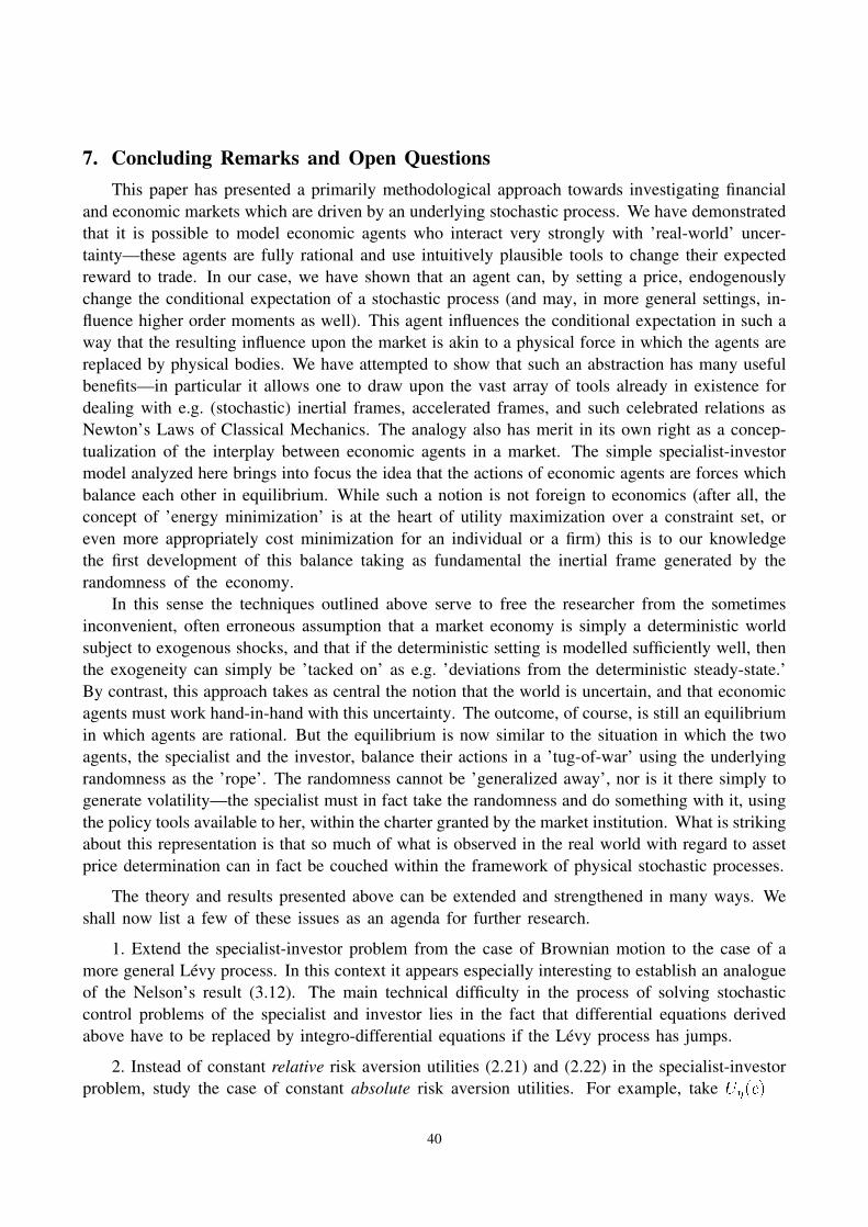
7. Concluding Remarks and Open Questions

This paper has presented a primarily methodological approach towards investigating financial

and economic markets which are driven by an underlying stochastic process. We have demonstrated

that it is possible to model economic agents who interact very strongly with ’real-world’ uncer-

tainty—these agents are fully rational and use intuitively plausible tools to change their expected

reward to trade. In our case, we have shown that an agent can, by setting a price, endogenously

change the conditional expectation of a stochastic process (and may, in more general settings, in-

fluence higher order moments as well). This agent influences the conditional expectation in such a

way that the resulting influence upon the market is akin to a physical force in which the agents are

replaced by physical bodies. We have attempted to show that such an abstraction has many useful

benefits—in particular it allows one to draw upon the vast array of tools already in existence for

dealing with e.g. (stochastic) inertial frames, accelerated frames, and such celebrated relations as

Newton’s Laws of Classical Mechanics. The analogy also has merit in its own right as a concep-

tualization of the interplay between economic agents in a market. The simple specialist-investor

model analyzed here brings into focus the idea that the actions of economic agents are forces which

balance each other in equilibrium. While such a notion is not foreign to economics (after all, the

concept of ’energy minimization’ is at the heart of utility maximization over a constraint set, or

even more appropriately cost minimization for an individual or a firm) this is to our knowledge

the first development of this balance taking as fundamental the inertial frame generated by the

randomness of the economy.

In this sense the techniques outlined above serve to free the researcher from the sometimes

inconvenient, often erroneous assumption that a market economy is simply a deterministic world

subject to exogenous shocks, and that if the deterministic setting is modelled sufficiently well, then

the exogeneity can simply be ’tacked on’ as e.g. ’deviations from the deterministic steady-state.’

By contrast, this approach takes as central the notion that the world is uncertain, and that economic

agents must work hand-in-hand with this uncertainty. The outcome, of course, is still an equilibrium

in which agents are rational. But the equilibrium is now similar to the situation in which the two

agents, the specialist and the investor, balance their actions in a ’tug-of-war’ using the underlying

randomness as the ’rope’. The randomness cannot be ’generalized away’, nor is it there simply to

generate volatility—the specialist must in fact take the randomness and do something with it, using

the policy tools available to her, within the charter granted by the market institution. What is striking

about this representation is that so much of what is observed in the real world with regard to asset

price determination can in fact be couched within the framework of physical stochastic processes.

The theory and results presented above can be extended and strengthened in many ways. We

shall now list a few of these issues as an agenda for further research.

1. Extend the specialist-investor problem from the case of Brownian motion to the case of a

more general Levy process. In this context it appears especially interesting to establish an analogue

of the Nelson’s result (3.12). The main technical difficulty in the process of solving stochastic

control problems of the specialist and investor lies in the fact that differential equations derived

above have to be replaced by integro-differential equations if the Levy process has jumps.

2. Instead of constant relative risk aversion utilities (2.21) and (2.22) in the specialist-investor

problem, study the case of constant absolute risk aversion utilities. For example, take U�(c) =

40

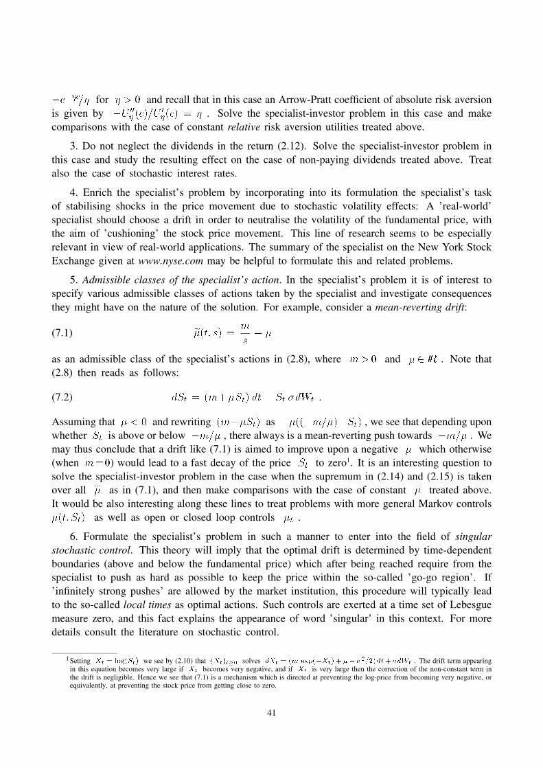
�e��c=� for � > 0 and recall that in this case an Arrow-Pratt coefficient of absolute risk aversion

is given by �U 00� (c)=U

0�(c) = � . Solve the specialist-investor problem in this case and make

comparisons with the case of constant relative risk aversion utilities treated above.

3. Do not neglect the dividends in the return (2.12). Solve the specialist-investor problem in

this case and study the resulting effect on the case of non-paying dividends treated above. Treat

also the case of stochastic interest rates.

4. Enrich the specialist’s problem by incorporating into its formulation the specialist’s task

of stabilising shocks in the price movement due to stochastic volatility effects: A ’real-world’

specialist should choose a drift in order to neutralise the volatility of the fundamental price, with

the aim of ’cushioning’ the stock price movement. This line of research seems to be especially

relevant in view of real-world applications. The summary of the specialist on the New York Stock

Exchange given at www.nyse.com may be helpful to formulate this and related problems.

5. Admissible classes of the specialist’s action. In the specialist’s problem it is of interest to

specify various admissible classes of actions taken by the specialist and investigate consequences

they might have on the nature of the solution. For example, consider a mean-reverting drift:

(7.1) e�(t; s) = m

s+ �

as an admissible class of the specialist’s actions in (2.8), where m> 0 and �2 IR . Note that

(2.8) then reads as follows:

(7.2) dSt = (m+�St) dt + St �dWt .

Assuming that � < 0 and rewriting (m+�St) as ��((�m=�)�St) , we see that depending upon

whether St is above or below �m=� , there always is a mean-reverting push towards �m=� . We

may thus conclude that a drift like (7.1) is aimed to improve upon a negative � which otherwise

(when m=0) would lead to a fast decay of the price St to zero1. It is an interesting question to

solve the specialist-investor problem in the case when the supremum in (2.14) and (2.15) is taken

over all e� as in (7.1), and then make comparisons with the case of constant � treated above.

It would be also interesting along these lines to treat problems with more general Markov controls

�(t; St) as well as open or closed loop controls �t .

6. Formulate the specialist’s problem in such a manner to enter into the field of singular

stochastic control. This theory will imply that the optimal drift is determined by time-dependent

boundaries (above and below the fundamental price) which after being reached require from the

specialist to push as hard as possible to keep the price within the so-called ’go-go region’. If

’infinitely strong pushes’ are allowed by the market institution, this procedure will typically lead

to the so-called local times as optimal actions. Such controls are exerted at a time set of Lebesgue

measure zero, and this fact explains the appearance of word ’singular’ in this context. For more

details consult the literature on stochastic control.

1 Setting Xt = log(St) we see by (2.10) that (Xt)t�0 solves dXt = (m exp(�Xt) + �� �2=2)dt+ �dWt . The drift term appearingin this equation becomes very large if Xt becomes very negative, and if Xt is very large then the correction of the non-constant term inthe drift is negligible. Hence we see that (7.1) is a mechanism which is directed at preventing the log-price from becoming very negative, orequivalently, at preventing the stock price from getting close to zero.

41

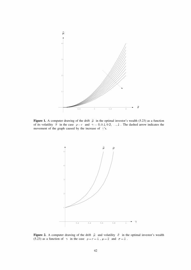
0.5 1 1.5 2

1

2

3

4

b�

b�Figure 1. A computer drawing of the drift b� in the optimal investor’s wealth (5.23) as a function

of its volatility b� in the case �= r and = 0; 0:1; 0:2; . . . ; 1 . The dashed arrow indicates the

movement of the graph caused by the increase of ’s.

0.2 0.4 0.6 0.8 1

1

2

3

4

5

b� b�

Figure 2. A computer drawing of the drift b� and volatility b� in the optimal investor’s wealth

(5.23) as a function of in the case �= r=1 , �=2 and �=1 .

42

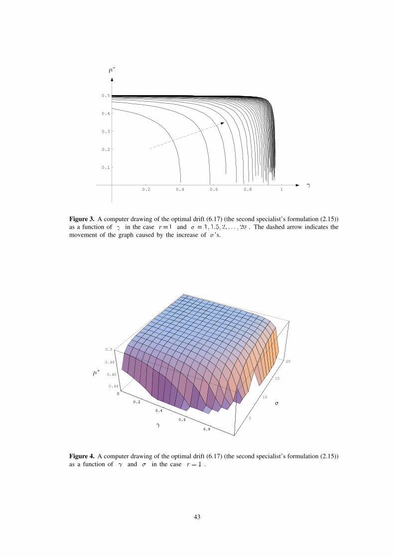
0.2 0.4 0.6 0.8 1

0.1

0.2

0.3

0.4

0.5

��

Figure 3. A computer drawing of the optimal drift (6.17) (the second specialist’s formulation (2.15))

as a function of in the case r=1 and � = 1; 1:5; 2; . . . ; 20 . The dashed arrow indicates the

movement of the graph caused by the increase of �’s.

0

0.2

0.4

0.6

0.8

5

10

15

20

0.44

0.46

0.48

0.5

0

0.2

0.4

0.6

0.8

��

�

Figure 4. A computer drawing of the optimal drift (6.17) (the second specialist’s formulation (2.15))

as a function of and � in the case r = 1 .

43

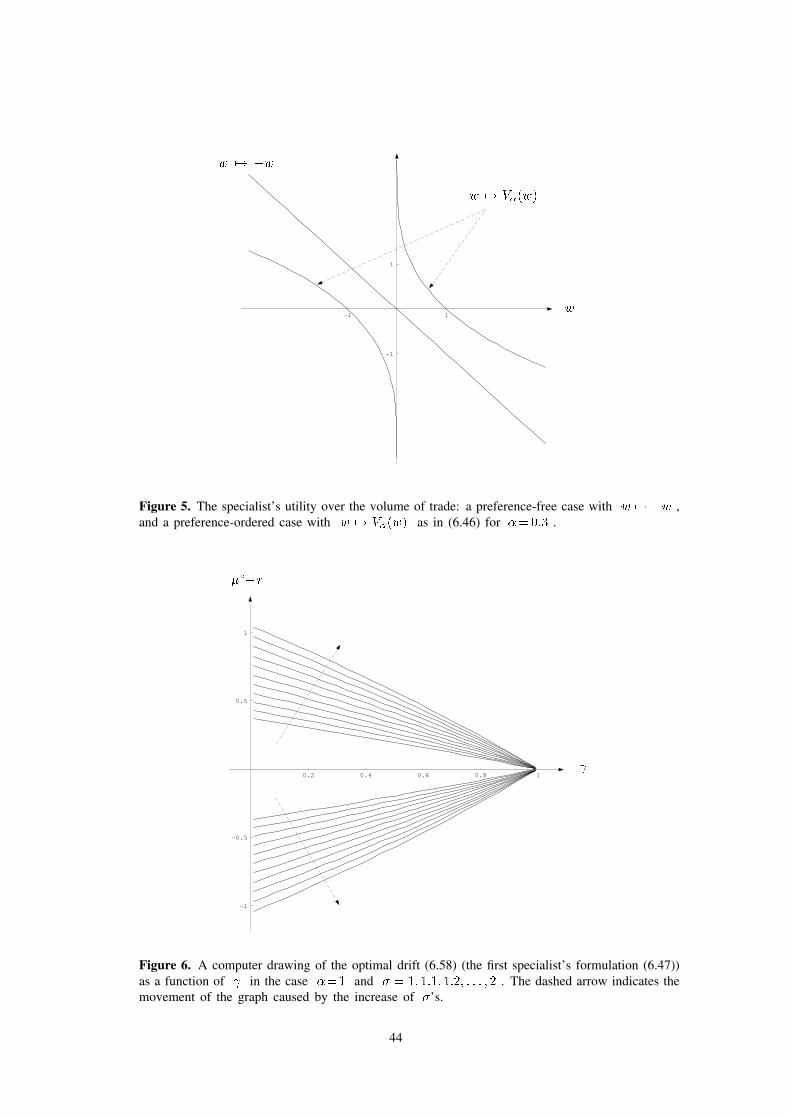
-1 1

-1

1

w 7! �w

w 7! V�(w)

w

Figure 5. The specialist’s utility over the volume of trade: a preference-free case with w 7! �w ,

and a preference-ordered case with w 7! V�(w) as in (6.46) for �=0:3 .

0.2 0.4 0.6 0.8 1

-1

-0.5

0.5

1

���r

Figure 6. A computer drawing of the optimal drift (6.58) (the first specialist’s formulation (6.47))

as a function of in the case �=1 and � = 1; 1:1; 1:2; . . . ; 2 . The dashed arrow indicates the

movement of the graph caused by the increase of �’s.

44

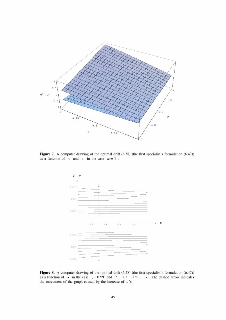
0

0.25

0.5

0.75

1

1

1.25

1.5

1.75

2

-1

-0.5

0

0.5

1

0

0.25

0.5

0.75

��� r

�

Figure 7. A computer drawing of the optimal drift (6.58) (the first specialist’s formulation (6.47))

as a function of and � in the case � = 1 .

0.2 0.4 0.6 0.8 1

-0.0015

-0.001

-0.0005

0.0005

0.001

0.0015

���r

�

Figure 8. A computer drawing of the optimal drift (6.58) (the first specialist’s formulation (6.47))

as a function of � in the case =0:99 and � = 1; 1:1; 1:2; . . . ; 2 . The dashed arrow indicates

the movement of the graph caused by the increase of �’s.

45

0

0.25

0.5

0.75

1

1

1.25

1.5

1.75

2

-0.001

0

0.001

0

0.25

0.5

0.75

��� r

�

�

Figure 9. A computer drawing of the optimal drift (6.58) (the first specialist’s formulation (6.47))

as a function of � and � in the case = 0:99 .

0

0.25

0.5

0.75

1

0

0.25

0.5

0.75

1

-0.2

0

0.2

0

0.25

0.5

0.75

��� r

�

Figure 10. A computer drawing of the optimal drift (6.58) (the first specialist’s formulation (6.47))

as a function of � and in the case � = 1 .

46

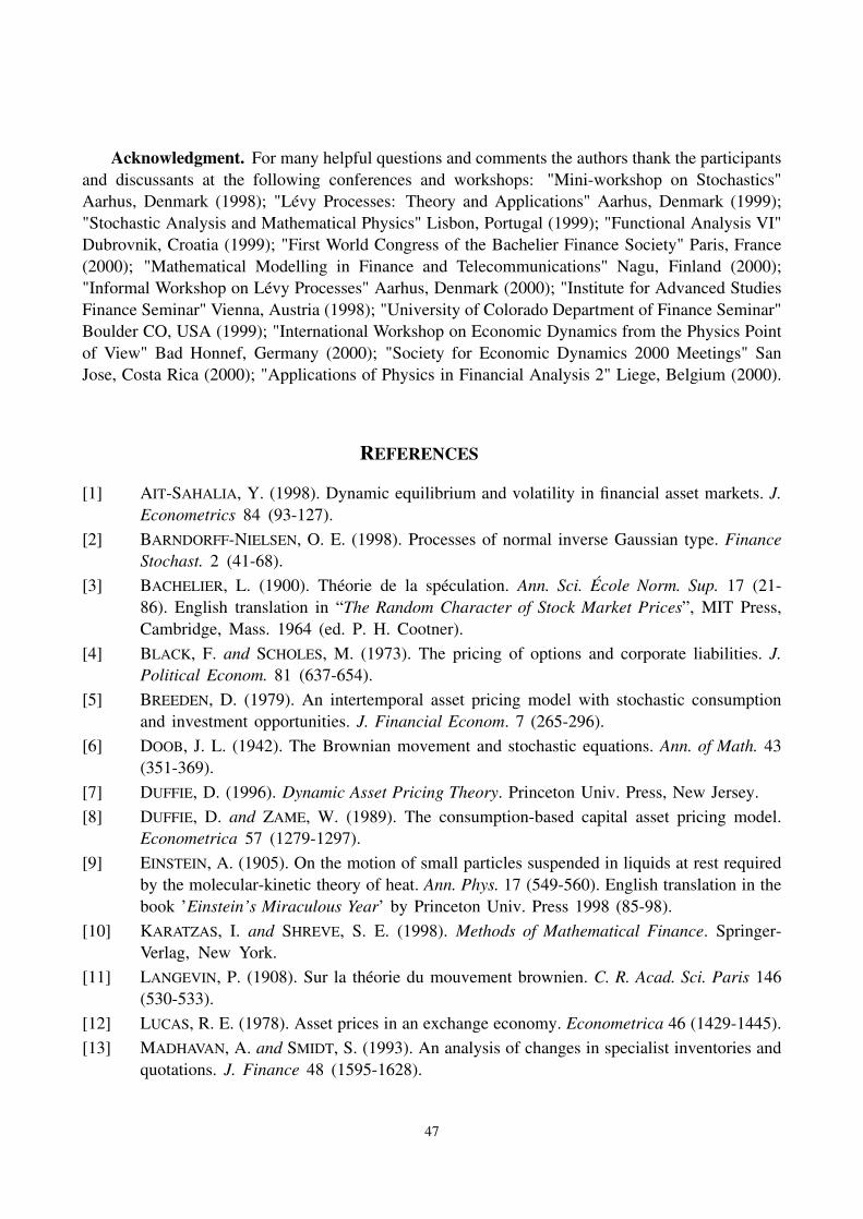
Acknowledgment. For many helpful questions and comments the authors thank the participants

and discussants at the following conferences and workshops: "Mini-workshop on Stochastics"

Aarhus, Denmark (1998); "Levy Processes: Theory and Applications" Aarhus, Denmark (1999);

"Stochastic Analysis and Mathematical Physics" Lisbon, Portugal (1999); "Functional Analysis VI"

Dubrovnik, Croatia (1999); "First World Congress of the Bachelier Finance Society" Paris, France

(2000); "Mathematical Modelling in Finance and Telecommunications" Nagu, Finland (2000);

"Informal Workshop on Levy Processes" Aarhus, Denmark (2000); "Institute for Advanced Studies

Finance Seminar" Vienna, Austria (1998); "University of Colorado Department of Finance Seminar"

Boulder CO, USA (1999); "International Workshop on Economic Dynamics from the Physics Point

of View" Bad Honnef, Germany (2000); "Society for Economic Dynamics 2000 Meetings" San

Jose, Costa Rica (2000); "Applications of Physics in Financial Analysis 2" Liege, Belgium (2000).

REFERENCES

[1] AIT-SAHALIA, Y. (1998). Dynamic equilibrium and volatility in financial asset markets. J.

Econometrics 84 (93-127).

[2] BARNDORFF-NIELSEN, O. E. (1998). Processes of normal inverse Gaussian type. Finance

Stochast. 2 (41-68).

[3] BACHELIER, L. (1900). Theorie de la speculation. Ann. Sci. Ecole Norm. Sup. 17 (21-

86). English translation in “The Random Character of Stock Market Prices”, MIT Press,

Cambridge, Mass. 1964 (ed. P. H. Cootner).

[4] BLACK, F. and SCHOLES, M. (1973). The pricing of options and corporate liabilities. J.

Political Econom. 81 (637-654).

[5] BREEDEN, D. (1979). An intertemporal asset pricing model with stochastic consumption

and investment opportunities. J. Financial Econom. 7 (265-296).

[6] DOOB, J. L. (1942). The Brownian movement and stochastic equations. Ann. of Math. 43

(351-369).

[7] DUFFIE, D. (1996). Dynamic Asset Pricing Theory. Princeton Univ. Press, New Jersey.

[8] DUFFIE, D. and ZAME, W. (1989). The consumption-based capital asset pricing model.

Econometrica 57 (1279-1297).

[9] EINSTEIN, A. (1905). On the motion of small particles suspended in liquids at rest required

by the molecular-kinetic theory of heat. Ann. Phys. 17 (549-560). English translation in the

book ’Einstein’s Miraculous Year’ by Princeton Univ. Press 1998 (85-98).

[10] KARATZAS, I. and SHREVE, S. E. (1998). Methods of Mathematical Finance. Springer-

Verlag, New York.

[11] LANGEVIN, P. (1908). Sur la theorie du mouvement brownien. C. R. Acad. Sci. Paris 146

(530-533).

[12] LUCAS, R. E. (1978). Asset prices in an exchange economy. Econometrica 46 (1429-1445).

[13] MADHAVAN, A. and SMIDT, S. (1993). An analysis of changes in specialist inventories and

quotations. J. Finance 48 (1595-1628).

47

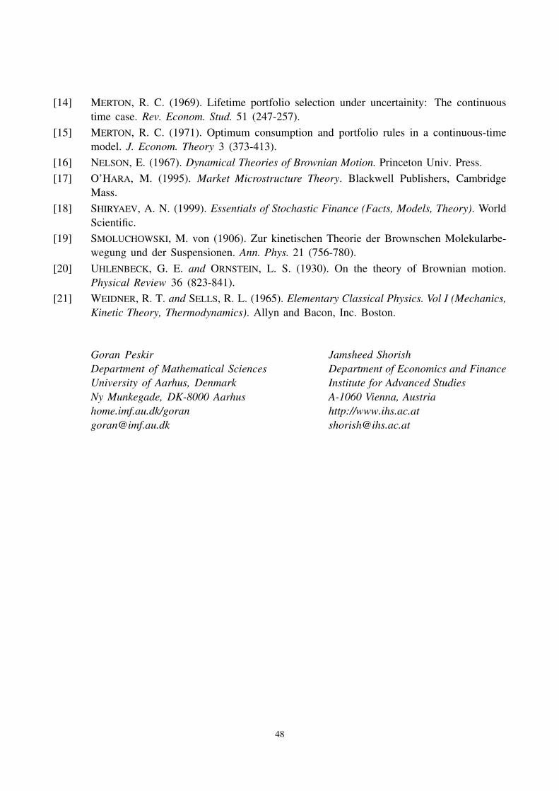
[14] MERTON, R. C. (1969). Lifetime portfolio selection under uncertainity: The continuous

time case. Rev. Econom. Stud. 51 (247-257).

[15] MERTON, R. C. (1971). Optimum consumption and portfolio rules in a continuous-time

model. J. Econom. Theory 3 (373-413).

[16] NELSON, E. (1967). Dynamical Theories of Brownian Motion. Princeton Univ. Press.

[17] O’HARA, M. (1995). Market Microstructure Theory. Blackwell Publishers, Cambridge

Mass.

[18] SHIRYAEV, A. N. (1999). Essentials of Stochastic Finance (Facts, Models, Theory). World

Scientific.

[19] SMOLUCHOWSKI, M. von (1906). Zur kinetischen Theorie der Brownschen Molekularbe-

wegung und der Suspensionen. Ann. Phys. 21 (756-780).

[20] UHLENBECK, G. E. and ORNSTEIN, L. S. (1930). On the theory of Brownian motion.

Physical Review 36 (823-841).

[21] WEIDNER, R. T. and SELLS, R. L. (1965). Elementary Classical Physics. Vol I (Mechanics,

Kinetic Theory, Thermodynamics). Allyn and Bacon, Inc. Boston.

Goran Peskir

Department of Mathematical Sciences

University of Aarhus, Denmark

Ny Munkegade, DK-8000 Aarhus

home.imf.au.dk/goran

goran@imf.au.dk

Jamsheed Shorish

Department of Economics and Finance

Institute for Advanced Studies

A-1060 Vienna, Austria

http://www.ihs.ac.at

shorish@ihs.ac.at

48