1

Market design with centralised wind power management:

handling low-predictability in intraday markets

Arthur HENRIOT1

Abstract:

This paper evaluates the benefits for an agent managing the wind power production within a given

power system to trade in the intraday electricity markets, in a context of massive penetration of

intermittent renewables. Using a simple analytical model we find out that there are situations when it

will be costly for this agent to adjust its positions in intraday markets. A first key factor is of course

the technical flexibility of the power system: if highly flexible units provide energy at very low prices

in real-time there is no point in participating into intraday markets. Besides, we identify the way wind

production forecast errors evolve constitutes another essential, although less obvious, key-factor. Both

the value of the standard error and the correlation between forecasts errors at different gate closures

will determine the strategy of the wind power manager. Policy implications of our results are the

following: low liquidity in intraday markets will be unavoidable for given sets of technical

parameters, it will also be inefficient in some cases to set discrete auctions in intraday markets, and

compelling players to adjust their position in intraday markets will then generate additional costs.

Keywords: Market design, intraday markets, wind forecasts, large-scale renewables, intermittency

1 Research assistant at Florence School of Regulation, Villa La Fonte - Via delle Fontanelle, 10 – 50014 San

Domenico di Fiesole (FI) –Italy. Email: arthur.henriot@eui.eu

The author would like to thank Jean-Michel Glachant, Vincent Rious, Haikel Khalfallah, Marcelo Saguan, the

editor and three anonymous referees for their highly capable help. Valuable comments were also provided

during the YEEES seminar that took place in spring 2012. All errors remain of course the author’s own

responsibility.

2

1. Introduction

The integration of a significant share of variable renewables in the electricity generation mix is a

source of economic and technical challenges. Wind generation variability and low-predictability

constitute a major obstacle to the integration of wind farms into electricity markets2.

We study in this article the case when intermittent RES are not isolated form electricity markets and

considered as a standard generator and we focus on one of the possible solutions to manage the low

predictability of electricity generation by wind farms: the use of Intraday Markets (IM). Wind

forecasts improve significantly when realised closer to generation. Giving generators a chance to

adjust in the IM their commitments realised in the Day-Ahead markets could help renewables to lower

their imbalance costs.

Intraday markets give players an opportunity to trade and to modify their production schedules after

the day-ahead gate-closure. They are already in place in most European countries but their design is

subject to significant variations. They can in particular be continuous (Germany, Denmark, France) or

feature discrete auctions (Spain, Italy). Despite wind already representing a significant share of

generated electricity in several countries, liquidity in IM remains low and the share of electricity

traded in IM is quite incidental3. Complementary rules have sometimes been put into place to increase

liquidity. For instance, from January 1, 2010, TSOs are required in Germany to balance any difference

between volumes of power from renewable sources sold in the Day-Ahead auction and the feed-in

based on the intraday forecast (Besnier, 2009). While such a regulatory measure will lead to a higher

liquidity in the IM, we argue it could also lead to additional costs. The purpose of this article is to

study under what conditions it will be beneficial for wind generators to trade in IM to manage wind

low-predictability.

2 For more details, the reader can for instance refer to the recent study by MIT: Perez-Arriaga, I.J., 2012.

Managing large scale penetration of intermittent renewables. MIT. 3 In 2009, the volume traded within the organised IM in Germany was 4.2% of the volume traded in the

organised Day-Ahead market. For the same year in Spain, the volume traded in the MIBEL IM was under 16%

of the total volume traded within the organised markets. (Source: Barquin et al. 2011)

3

We build a simple analytical model to study how the prediction error for electricity generated by wind

farms for a given generation time can be managed in IM. In order to focus on the effects of low-

predictability for a single hour, we do not consider interdependency between adjacent generation

times. We suppose wind generators are aggregated into a single player who commits to generate a

given quantity in Day-Ahead markets. Due to forecast errors, this player is exposed to imbalance costs

when the actual output is different from its financial position. This player is also given the possibility

to adjust its commitments by interacting with thermal generators4 at a set of gates within the IM. We

also introduce a parameter to take into account the system flexibility in our model. Due to the limited

technical flexibility of thermal generators, it is more expensive to procure energy on short-notice5.

We use this model to study the average profits of a wind power producer using the best predictions

available to adjust its position in selected gates from IM and compare it to the average profits realised

by a producer adopting a more passive attitude. It is less expensive to manage imbalances earlier, but

there is a risk of correcting self-compensating deviations. This process allows us to establish a set of

critical values for the technical properties of the forecast error. Relevant parameters include standard

error, correlation between errors at different times, and additional costs of purchasing electricity

closer to real-time. Our results indicate that the value of these parameters will determine whether it is

a good strategy for the producer to use updated predictions to trade in the intraday market at a given

time. As these parameters evolve with each gate-closure time, setting discrete auctions at a sub-

optimal time will deter participants from trading within this time period.

2. Previous works

Despite the relatively low volume of electricity currently traded in intraday markets, their alleged

potential to assist the integration of intermittent renewables such as wind led to the development of a

range of studies focusing on this topic. For example, Borggrefe and Neuhoff (2011) and Hiroux and

4 In this article, the term “thermal generators” is used to refer to all units considered as having a predictable

output. Thus large hydropower can also be included in this abusive simplification. 5 According to a recent study by the MIT Energy Initiative (2012), nuclear plants (featuring low marginal costs)

require six to eight hours to ramp up to full load, while coal plants can ramp their output at 1.5%-3% per minute.

The most flexible coal units are the smaller and older plants with less efficiency.

4

Saguan (2010) both mentioned the use of IM to manage wind low-predictability. Borggrefe and

Neuhoff (2011) presented intraday markets as a tool to keep the volume of balancing services low in

systems featuring a significant penetration of intermittent renewables but did not consider oscillating

predictions6. Hiroux and Saguan (2010) argued setting the gate closure that closes intraday markets

near real-time would help to reduce wind integration balancing costs.

A first category of studies focusing on the IM consists of empirical analysis of players’ participation

in IM, such as Weber (2010) and Furió et al. (2009). Weber (2010) focused on the volume exchanged

in several European Intraday Markets. He estimated a theoretical potential for position adjustments of

wind generators in intraday markets and deduced that the amount of exchanges reached in these

markets were quite low when compared to this potential. Weber (2010) distinguished two possible

explanations for poor liquidity. A first reason could be poor market design. In this case, it can

moreover become a self-sustaining phenomenon, as the absence of liquidity reduces the trust of

participants into IM. Another possible explanation can be the absence of a real need for IM, i.e. a

question of market structure7. There is a fundamental difference between these two drivers with

consequences regarding policies to adopt. Yet no clear conclusion was reached regarding the exact

source of low liquidity. Furió et al. (2009) realised a statistical analysis of trades made in the Spanish

Intraday markets. This study revealed that about two thirds of the exchanges realised within each of

the six trading sessions were linked to the hourly horizons negotiated for the last time in this session.

Most of the time only one gate out of six was really used by participants. They furthermore added the

low liquidity calculated could be due to an absence of need to make adjustments in the IM.

A second category of studies features models to estimate the value for wind power generators of

trading into intraday markets. Usaola and Angarita (2007) considered three possible strategies in IM:

no bidding, bidding best prediction, and an “optimal” strategic bidding. The frame was the Spanish

IM, prices were inputs based on historical data, and only one intermediate step was considered in the

6 The term “oscillating predictions” refers to the case when the successive updated forecasts for the same

generation time are alternatively increasing and decreasing when getting closer to real-time. 7 Stoft (2002) for instance employed “market structure” by opposition to “market architecture” to refer to

properties of the market closely tied to technology and ownership. We will stick to this definition in this article.

5

IM. Results indicated bidding the best prediction was not the optimal strategy and that it was

sometimes even preferable not to play at all in IM. Similar results were obtained by De Vos et al.

(2011) in the Belgian context. Day-Ahead (DA) and Balancing Mechanism (BM) prices were inputs

taken from the Belgium Power Exchange BELPEX while IM prices were estimated through linear

interpolation between DA and BM prices. Increasing total balancing costs resulting from trading into

IM were explained by oscillating predictions. Maupas (2008) employed a quite sophisticated approach

using a power system simulation and modelling the interaction between intraday and balancing

markets. He established that it was not beneficial to trade into IM with poor liquidity due to

interactions between the different hourly provision horizons. In Maupas’ model, poor liquidity was

an exogenous input taken into consideration by setting intraday market prices closer to the BM prices

than to the DA prices.

While wind and intraday markets have hence been subject to different approaches, we believe there is

room for further investigation. While there seems to be a general intuition in the studies mentioned in

this section that trading in IM could result in higher costs in case of poor liquidity and oscillating

predictions, the calculations made so far did not establish for what kind of forecast precision and for

what market flexibility it was the case. By using a simpler analytical model, we might not be able to

deliver accurate numerical results but we will be able to focus on the role played by two key technical

components: forecast accuracy and system flexibility.

3. Model

3.1. Modelling framework

In our analytical model, wind generators are aggregated into a single player. This player could

represent a utility operating the totality of wind power plants, a national aggregator, or a TSO

responsible for managing wind intermittency as it is the case in Germany. Our results can be applied

to any system featuring one of these structures.

6

Our player generates energy using installed wind capacity and is also able to procure energy from

thermal generators in electricity markets. At the gate-closure time of the day-ahead market, this player

plans to generate a given quantity of wind energy for a final production horizon. However due to

imperfect forecast, the final output will be different from the player position. This “wind player” will

therefore need to manage imbalances.

We compare different strategies in our model ranging from a completely passive strategy to an

extremely active strategy. A completely passive strategy is to “do nothing” and pay the balancing

costs when the final production is realised: this is the case when it is not possible to trade into IM or

when the player is not taking part into these markets. An extremely active strategy is to use the

updated forecast available at each gate of the IM: the wind player will then be interacting with the

thermal generators to adjust its positions8. As a result, the active player will need to buy or sell less

energy in balancing markets (only the remaining error at the last intraday market gate closure) but

might buy and sell more energy in the intraday markets due to oscillating predictions. The completely

passive strategy and the extremely active strategy constitute the two extreme possibilities of a much

more complex set of strategies: in practice, in our model, at each available gate of the IM, the player

can choose whether to adjust its position using the best available forecast. This is illustrated in Figure

1.

We assume that the evolution of the system imbalance is driven by the wind manager generation

imbalances, which is a reasonable assumption in a system featuring a significant share of variable

renewables managed by a single player9. Indeed while load is also uncertain the errors will then be

smaller and their evolution is easier to anticipate (Maupas, 2008).

8 If the updated forecast indicates a higher output than the previous forecast the wind player can sell more

energy. If the updated wind forecast indicates a lower output the wind player must buy energy.

9 The assumption that a single player is managing the whole wind power generation is therefore a key

assumption in our discussion. Our results would however remain qualitatively true with a significantly dominant

player or for any player whose imbalances are strongly positively correlated to the total system imbalances.

7

Figure 1: Illustration of two possible strategies: the player chooses to participate in IM at gates H-24, H-12, H-4 and

H-2 (left side) vs. the player decides not to participate at all in IM (right side).

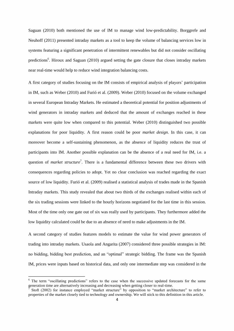
Thermal generators have a limited flexibility. The least flexible plants will not be able to adapt their

production to the demand when getting closer to the production horizon or will only be able to adapt it

in a restricted way respecting ramping constraints. They will therefore withdraw part of their offers

from the supply function, as illustrated in Figure 2. The resulting inverse supply function will

therefore feature a steeper slope, and prices will get more expensive when getting closer to the

production horizon10

. Moreover, the units most likely to provide the required flexibility to manage

wind variability are usually the ones with high marginal costs11

(see IEA (2012)).

At last, energy procured in real-time is not always charged at cost-reflective prices (Vandezande et al.,

2010). Penalties can be imposed by the system operator to provide ex-ante balancing incentives to

participants. Such penalties could be included in our model by higher prices for energy procured and

lower revenues from selling energy in real-time markets. Due to these extra-costs, participants should

then have higher incentives to participate in intraday markets.

10

Exercise of market power could strengthen the impact of this phenomenon, as illustrated by Green and

Vasilakos (2010): when the residual demand for power production by flexible units is high, these units exercise

market power to a greater extent and prices rise.

11 It could be argued some very flexible power units, typically hydropower units, also feature low marginal

costs. However these generators, as they are the most flexible, can choose to sell their production at any time-

horizon. It is likely they will sell their production in earlier markets if prices are higher in these higher markets.

8

Figure 2: Evolution of the economic merit-order due to limited flexibility

3.2. Model implementation

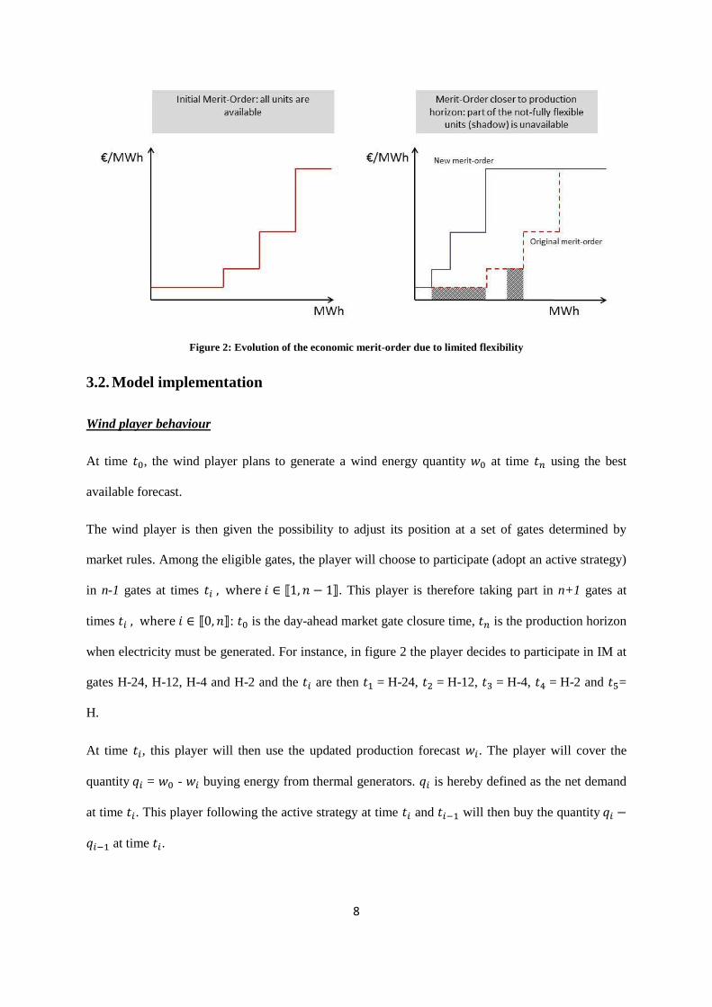
Wind player behaviour

At time , the wind player plans to generate a wind energy quantity at time using the best

available forecast.

The wind player is then given the possibility to adjust its position at a set of gates determined by

market rules. Among the eligible gates, the player will choose to participate (adopt an active strategy)

in n-1 gates at times ⟦ ⟧. This player is therefore taking part in n+1 gates at

times ⟦ ⟧: is the day-ahead market gate closure time, is the production horizon

when electricity must be generated. For instance, in figure 2 the player decides to participate in IM at

gates H-24, H-12, H-4 and H-2 and the are then = H-24, = H-12, = H-4, = H-2 and =

H.

At time , this player will then use the updated production forecast . The player will cover the

quantity = - buying energy from thermal generators. is hereby defined as the net demand

at time . This player following the active strategy at time and will then buy the quantity

at time .

9

At the final time , the wind player will cover the net demand and pay the corresponding

imbalance costs. A player having adopted the active strategy in gate will be charged the costs

corresponding to the remaining energy quantity . By opposition, a player having adopted

the passive strategy will be charged the costs corresponding to the energy quantity .

The quantities ⟦ ⟧ are random variables whose behaviour depends on the wind farms

characteristics and the wind nature itself. In order to make calculations simpler, we define the variable

representing the wind production forecast error at time as a share of the realised wind

production.

The resulting random variable has an expected value ( ) and a variance . We suppose

and are independent:

⟦ ⟧ ( )

This simplification is made under the assumption that the forecast error expressed as a share of the

realised wind production is not correlated to the realised wind production . In other words, there is

no systematic relationship between wind power generation and wind power prediction accuracy12

.

Moreover ( ) indicates there is no systematic underestimation or overestimation at a given

time. This is a very reasonable assumption as a forecasting tool presenting such a bias would be

adjusted.

Prices formation

In our model wind power producers interact with thermal generators to buy the extra energy they need

or to sell surplus energy. Demand-side is not considered as we suppose the balancing needs driven by

the consumption-forecast error will be insignificant in a power system featuring high penetration by

12

An example of empirical study analysing this property of wind power forecasts can be found in section 6 of Lange (2003).

10

intermittent RES13

. The available thermal generators obey at time to the following aggregated

inverse supply function. For a net demand , the corresponding price ( ) is:

( )

The price function is therefore linear and parameters a and b are inputs that depend on the power

system properties. The variable b will be higher when the range of marginal costs of the different

generation units will be higher.

The evolution of costs of dealing with imbalances will play a significant part in the trade-off wind

generators are to face. To take flexibility into account in our model we introduce a “penalty function”

( ). We assume the value of the penalty function ( ) increases with time t: the extra cost of trading

later is higher closer to real time.

We suppose a producer who committed at time to buy the quantity and trading the quantity

at time will pay a price ( ). The resulting price function obeys to the following

equation graphically illustrated in Figure 3 :

( ) ( ( ( )) ( ))

( ) ( ) ( ) ( )

In case the system is not perfectly flexible (i.e. ( ) ) the same quantity of electricity

bought later by wind generators (when generation by thermal units is higher) will be more costly,

while electricity sold later by wind generators (when generation by thermal units is lower) will lead

to lower profits.

13

While outages of thermal units will still be relevant for the network security we considered that due to the low

frequency of occurrence they could be neglected in our financial analysis.

11

Figure 3: Evolution of the inverse supply function in our model

It is important to point out that representing the classical stepwise merit-order curve by a linear merit-

order curve is a quite restrictive assumption. For a given time, in a real electricity market, start-up

costs and additional non-convexities might challenge this hypothesis. However the scope of this

article is to provide insights of phenomena taking place into IM, focusing on a single production hour.

In this context, we considered that neglecting non-convexities constituted a reasonable assumption.

The same argument also applies to the approximation by the supply function at different times .

Picking the best strategy

A wind power producer having chosen to participate in IM at times and will trade the quantity

at time and pay a price ( ). The total cost for a participants being active at

times ⟦ ⟧ will therefore be the sum of these transactions14

:

( ) ∑[ ( ) ( )]

By opposition a producer staying completely out of the intraday market (what we defined as the

passive strategy) will only buy the initial amount of energy at and pay the imbalance costs

corresponding to quantity at time The total cost will then be:

( ) ( ) ( )

14

We consider that transaction costs are not significant and can be neglected in this study.

12

The player considered will be risk-neutral in our analysis. In order to compare the efficiency of these

two strategies, the chosen active strategy and the passive strategy, we will have a look at the expected

value of the difference between these two total costs ( ).

( ) ( ( ) ( ))

We will then compare the case of a player only active at times with the case of the

player in addition active at time with . We will study the sign of

( ) ( ) to determine whether it is worth or not being

active at time in addition to .

4. Analytical results

4.1. General case

To express more precisely the value of ( ) it is necessary to introduce the correlation

coefficient between and defined as: ( )

It is then possible to show the following result (see Appendix for demonstration):

( ) ( ) [∑

∑

]

( ) (

)

( )

This result can deliver a few insights. First of all, the costs of picking the wrong strategy (whether it is

to play or not at a given time in intraday markets) will be proportional to both the slope of the supply

curve and the expected value of the square of wind power production ( ) It is important to point

out that ( ) is higher when the average production is higher but also when the variability of the

13

production is higher15

. In a system where wind production is steadier, for example because the wind is

itself more steady or because wind farms are more dispersed, the errors will also be less important. In

a system where the marginal costs of thermal plants, flexible or not, are roughly the same, it will

matter less which ones are called to generate.

Finally, the relevance of trading into these gates will be the result of a trade-off between the different

members of this equation. The terms are always positive and represent the “flexibility penalty” of

buying energy latter in intraday markets when the generator adopts the active strategy. The term

is always negative and represents the same penalty paid in case the wind generator adopts a passive

strategy. The value of the term depends on the system characteristics and can be either positive or

negative. If correlation between and is poor then losses resulting from oscillating

predictions will be high and it might not be worth trading in intraday markets.

4.2. Results in a simple case with one gate closure in the intraday market

In a recent study of the Spanish electricity market, Furió et al. (2009) estimated that about two thirds

of exchanges realised in the IM take place during the last possible platform. It means players use only

one gate of the IM for a given hour. It is therefore interesting, in addition to being a good educational

example, to study the case when the player is deciding whether to adjust its position (or not) at a

single gate between the day-ahead electricity market and the generation time.

15

Indeed ( ) = ( ( ))

( )

14

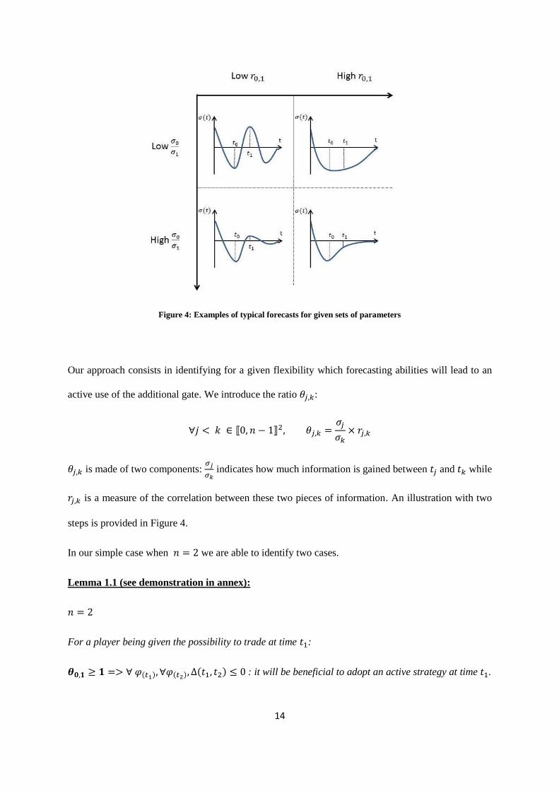
Figure 4: Examples of typical forecasts for given sets of parameters

Our approach consists in identifying for a given flexibility which forecasting abilities will lead to an

active use of the additional gate. We introduce the ratio :

⟦ ⟧

is made of two components:

indicates how much information is gained between and while

is a measure of the correlation between these two pieces of information. An illustration with two

steps is provided in Figure 4.

In our simple case when we are able to identify two cases.

Lemma 1.1 (see demonstration in annex):

For a player being given the possibility to trade at time :

( ) ( ) ( ) : it will be beneficial to adopt an active strategy at time .

15

Lemma 1.2 (see demonstration in annex):

For a player being given the possibility to trade at time :

/ ( ) ( ), ( ) : it will not be beneficial to adopt an

active approach at .

It is possible to go beyond these mathematical results and explore their meanings. In case

is low,

there is little interest in trading at since the forecast is not much more accurate. In case is low,

there is little interest in trading at as there are higher risks of spoiling energy due to oscillating

prediction errors. That’s why is a key parameter.

From lemma 1.1, it is interesting for the producer to anticipate imbalances at if the forecast error

evolution is good enough.

From Lemma 1.2, if the anticipation is not really helpful, i.e. is low, then it can be interesting or

not to anticipate imbalances. If imbalances are never very expensive it is not worth taking the risk of a

wrong anticipation.

4.3. Interest of trading at a given gate closure in the general case

Most intraday markets feature several gates (six in Spain) or allow continuous trading. Therefore we

will have a look in this section at a general case when a participant is adjusting its position in

gates in the IM at times ⟦ ⟧. We study the effects of being active at one more gate

at time and identify a set of criteria that will favour or discriminate against an active approach at

this gate. By extension it is then possible to determine in which case a continuous market will be fully

used by participants when tends to infinity.

Lemma 2.1 (see demonstration in annex):

For a player adopting an active strategy in IM at gate closure times being given

the possibility to trade at time with :

16

{

( ) ( ) : it will be beneficial to

adopt an active strategy at .

Lemma 2.2 (see demonstration in annex):

For a player adopting an active strategy in IM at gate closure times being given the

possibility to trade at time with :

{

( ) ( ) ( ) ( ) it will not

be beneficial to adopt an active approach at .

We can deduce from lemma 2.2 that for a given flexibility of the power system and a specific forecast

error evolution the active strategy might be more costly than the passive one. This result is coherent

with the results obtained by Maupas (2008), De Vos et al. (2011) and Usaola and Angarita (2007).

5. Results interpretation

5.1. Liquidity in intraday markets

Conclusion 1: Low liquidity in intraday markets will be unavoidable for a given set of technical

parameters.

A first insight we can get from our analysis is that poor liquidity in intraday markets may result from a

rational behaviour of the participants. Our results indeed indicate that the poor liquidity of intraday

markets could be explained by the poor information players have to deal with. Lemma 2.2 shows

oscillating predictions can deter the players from trading in the IM provided it is not too expensive to

procure energy in the balancing markets. This is an intuition already exposed by some of the authors

mentioned in the section 2 of this article, but our results enlighten the key role played by the

factor . When the value of this parameter is low, it means the gain of information when getting

closer to real-time is not sufficient to compensate the oscillating nature of wind forecasts. Participants

17

acting rationally will then choose not to adjust their positions between day-ahead markets and real-

time. Intraday markets will not be used by participants because they do not meet the needs of the

participants.

Conclusion 2: In some cases, compelling players to trade into intraday markets will generate

additional costs.

As long as conditions remain unsuitable, it will not be possible to increase both efficiency and

liquidity by changing rules. Compelling wind power generators to trade in the intraday markets will

mechanically lead to a more liquid intraday market, but these obligations can potentially result in

higher total balancing costs. Higher volumes should not be the objective of regulators. The volume of

exchanges in the intraday markets will spontaneously rise (or decrease) following a higher penetration

of renewables or technological changes. A prerequisite is obviously that the intraday markets must be

in place in the power system, even if they are not used by most participants. If the forecasting tools

become good enough, producers will then apply voluntarily what we defined as the active strategy, in

order to minimise their costs, as shown in lemma 2.1.

Similarly, setting penalties in real-time markets to incentivise participants to balance ex-ante their

positions will lead to a higher participation in intraday markets, as in practice the extra cost ( ) of

trading in real-time will increase. However the actual costs of generating electricity will not be

transformed by such financial penalties and these additional adjustments will not result in a higher

efficiency. Increased participation in intraday markets will then be a form of hedge against imbalances

with negative consequences similar to the ones described in Vandezande et al. (2010).

5.2. Trade-offs between continuous trading and discrete auctions

As mentioned in the introduction, there are two main options available to design intraday markets:

continuous markets and discrete auctions (Barquin et al., 2011). In a continuous market, bids are

matched one by one as soon as they match (i.e. when the bid price is higher than the offer price). The

main alternative consists in a set of discrete auctions.

18

Conclusion 3: Setting discrete auctions in intraday markets may lead to inefficiencies due to lost

trading opportunities.

By opposition to continuous markets, discrete auctions restrict trading to a set of pre-established

times. Yet we know from our analysis that the strategy of a player will differ at different times.

Depending on the wind forecast properties, a player might for instance be willing to trade at 10 a.m.

but not at 9 a.m. or 11a.m. In a continuous market, players can use the experience they acquired day

after day, and they will then be able to optimise their behaviour and trade when it is the most

interesting for them. In a discrete market players will not be given such freedom: if conditions are not

suitable (i.e. if the gates are set at times that do not fit this player) players will not trade, as shown by

lemma 2.2.

That’s why we argue restricting trading at imposed gates (as it is the case in an IM featuring discrete

auctions) may lead to inefficiencies, additional costs, and lost trading opportunities. This result shall

temper assumptions that discrete auctions will lead to increased trade in IM16

. Obviously there are

other sources of inefficiencies in continuous markets related to their inner fundamental properties: as

trades are made on a first-come first-served basis in a continuous market, some trades that would not

have taken place in a discrete market might take place, and the resulting prices will be less

transparent. However, the decision to put into place continuous or discrete intraday markets should

take into account the advantages of continuous markets that we described in addition to these

drawbacks.

It could be argued that the gate-closure times could be set in a way to reflect players’ preferences,

which would only be theoretically possible in the case of a single balancing responsible party. Gates

should in this case be set after analysing wind forecast evolutions and should be regularly updated as

forecasting technologies and the generation park evolve. Such a painful administrative process could

16

The case for discrete auctions is often illustrated by the relatively high liquidity in the Spanish intraday

markets. Yet it is important to take into account the fact that in the Spanish electricity market, portfolio bidding

is not allowed. Therefore, as underlined by Pérez Arriaga (2005), a significant share of the volumes exchanged

in the intraday markets is due to internal re-allocation by participants of the dispatch resulting from the daily

market. It is not the case in most other European electricity markets where portfolio bidding is implemented.

Therefore the case of the Spanish IM should be exploited carefully.

19

be avoided by putting into place continuous markets. The losses would then offset the potential

benefits from more efficient allocation in markets featuring discrete auctions.

6. Conclusion

In this paper, we assessed the different strategies that could be employed in intraday markets by

parties responsible for managing wind forecast error. Participants trading in intraday markets face a

trade-off: being exposed to imbalance charges or adjusting positions in the intraday market when

some relevant information is still missing. Therefore we developed a simple analytical model

allowing us to take into account both the system flexibility (as the lower the flexibility, the higher

imbalance charges) and the nature of the wind forecast evolution (as it determines the information

available to participants).

While discussions about optimal gate-closures usually focused on the average forecast error and the

system flexibility when getting closer to real-time we demonstrated that correlation between forecast

errors at different times should be taken into account. We were able to identify the parameter

reflecting both the oscillating nature of wind forecasts and the level of information gained when

getting closer to real-time. We showed this parameter plays a key-role in determining the participants’

strategies.

Our analytical results underlined the fact that oscillating predictions could indeed explain the poor

liquidity in IMs. In this case, a higher volume of exchanges in the intraday market should not be an

objective per se as poor liquidity could simply reflect the fact taking part into these intraday markets

will lead to higher costs: reducing total balancing costs should remain the main objective of regulated

TSOs and regulators when establishing rules.

Our analysis also revealed it was unlikely a set of gates would please all participants. Players

responsible for balancing wind low-predictability will achieve cost-optimisation spontaneously if they

are given the opportunity to trade when they need it. We argue continuous markets provide

participants with a sufficient degree of freedom to express their needs. While the liquidity remains

low in continuous markets in place in Europe it should yet become naturally higher with an increasing

20

share of renewables in the generation mix, as incentives to reduce costs should lead participants to

optimise their participation in intraday markets. Lost opportunities resulting from setting discrete

auctions might offset their benefits.

It must be pointed out that our model has been designed to provide general insights about the

behaviour of wind players in intraday markets. As a consequence, rather strong assumptions have

been employed, and the results obtained might therefore not be universally valid. Relaxing some of

the assumptions described in section 3 should however not impact our results significantly: for

instance start-up costs that we neglected tend to increase when getting closer to real-time and could be

internalised in the supply function. In this paper, it has also been considered that players are risk-

neutral. Risk-averse players might have stronger incentives to participate in IM (thus reducing their

exposure to imbalances in real-time markets) but our results should not be qualitatively impacted

when relaxing this assumption.

Another key-assumption we made is that wind power production is managed in a centralised way.

While this assumption is close to reality in some power systems (such as Germany) it might not

reflect the more complex situation in other power systems. This assumption is essential when

considering that the system total imbalances are driven by the sign of our player imbalances: however

our results will remain qualitatively true for any player whose imbalances are strongly (positively)

correlated with the total system imbalances. This will in particular be the case if the main wind power

producers own similar generation parks: a similar technology employed, in location with similar

properties. A possible extension of our work could be to consider the interactions of several players

managing only partly-correlated wind power sources.

21

Appendixes

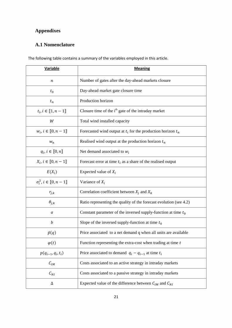
A.1 Nomenclature

The following table contains a summary of the variables employed in this article.

Variable Meaning

Number of gates after the day-ahead markets closure

Day-ahead market gate closure time

Production horizon

⟦ ⟧ Closure time of the ith gate of the intraday market

Total wind installed capacity

, ⟦ ⟧ Forecasted wind output at for the production horizon

Realised wind output at the production horizon

, ⟦ ⟧ Net demand associated to

, ⟦ ⟧ Forecast error at time as a share of the realised output

( ) Expected value of

, ⟦ ⟧ Variance of

Correlation coefficient between and

Ratio representing the quality of the forecast evolution (see 4.2)

a Constant parameter of the inversed supply-function at time

b Slope of the inversed supply-function at time

( ) Price associated to a net demand q when all units are available

( ) Function representing the extra-cost when trading at time

( ) Price associated to demand at time

Costs associated to an active strategy in intraday markets

Costs associated to a passive strategy in intraday markets

Expected value of the difference between and

22

A.2: Expression of ( )

( ) (∑[ ( ) ( )]

( ) ( )) (1)

By definition,

( ) ( ( ( )) ( )) (2)

And

( ) (3)

Thus by developing (1) we obtain:

( ) (∑ [ ( )] ∑ [ ( ) ( )

] )

( ( ) ( ) ( ) )

(4)

We will then estimate each of the four members of this equation

( ( )) ((

) (

)

)

As, by definition, and ( ) ( )

( ( )) ((

) (

)

)

Thus following notations defined in 3.2 we obtain:

( ( )) (( ) ( ) )

And as by assumption (see section 3.2) ⟦ ⟧ ( ) and ( )

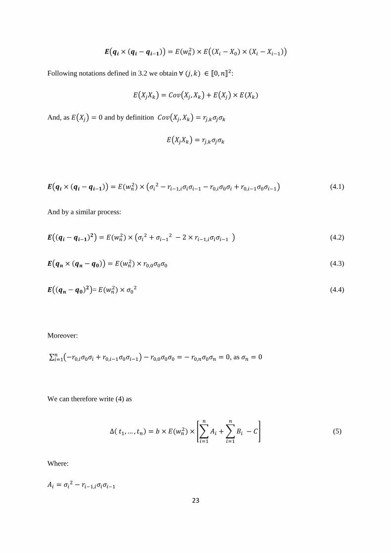
23

( ( )) ( ) (( ) ( ))

Following notations defined in 3.2 we obtain ( ) ⟦ ⟧ :

( ) ( ) ( ) ( )

And, as ( ) and by definition ( )

( )

( ( )) ( ) (

) (4.1)

And by a similar process:

(( ) ) (

) (

) (4.2)

( ( )) ( ) (4.3)

(( ) )= (

) (4.4)

Moreover:

∑ ( ) , as

We can therefore write (4) as

( ) ( ) [∑

∑

] (5)

Where:

24

( ) (

)

( )

A.3: Proof of lemma 1.1:

We apply equation (5) in the special case when

( )

( ))

( ) (

) ( )

( )

(6)

As | |

( )

Hence ( ) ( ) ( ) (

)

(7)

We assume that

: the uncertainty increases with the prediction horizon.

If we assume we obtain the following results:

(7.1)

And as

( )

(

)

(7.2)

We also know that ( ) ( ) as the flexibility penalty ( ) increases with

( ) ( ) (8)

Using (7.1), (7.2) and (8) we can show that the following equation is verified

25

( ) ( ) (

)

(9)

And according to (7) and (9), ( )

A.4: Proof of lemma 1.2:

We assume

By analogy to the proofs of (7.1) and (7.2), we can show:

(10.1)

(

)

(10.2)

And therefore:

/ ( ) ( ) (

)

(11)

As by definition ( )

/ ( ) ( ) ( ) (

)

(12)

Using (7), / ( ) ( ), ( )

A.5: Proof of lemma 2.1:

A player adopting an active strategy in IM at gate closure times is being given the

possibility to trade at time with

26

We make two assumptions.

Assumption 1:

Assumption 2:

By definition it will be beneficial to adopt an active strategy at if and if only:

( ) ( ) (13)

Most of the terms are present on each side and by developing and simplifying (13) is equivalent to

( ) (

)

( ) (

) (14)

Under assumption 1, and therefore

(15.1)

In addition we know that we assumed greater uncertainty further away from the production horizon:

(15.2)

Using (15.1) and (15.2)

(16)

And according to (16) it is possible to rewrite ( ) as:

( ) ( )

(17)

We know have to show that inequality (17) is true to ensure that inequality (13) is true.

Under assumption 2:

27

Under assumption 1:

(18.1)

Besides

As ,

(18.2)

We also know that by definition ( ) ( ) as the flexibility penalty ( ) increases with

Hence using (18.1) and (18.2):

( ) ( )

(19)

And (17) is verified, which is equivalent to ( ) ( ): it is

beneficial to play the active strategy.

A.6: Proof of lemma 2.2:

Similar to 1.2 using equation (17).

28

References

Barquin, J., Rouco, L., Rivero, E., 2011. Current designs and expected evolutions of Day-ahead, Intra-day and balancing market/mechanisms in Europe, in: OPTIMATE (Ed.). Besnier, D., 2009. Impact of the law on Renewable Energy ("EEG") on EPEX Spot German/Austrian Auction, EPEX SPOT INFO. Borggrefe, Neuhoff, K., 2011. Balancing and intra-day market design: options for wind integration, in: Initiative, C.P. (Ed.), European Smart Power Market Project. De Vos, K., De Rijcke, S., Driesen, J., Kyriazis, A., 2011. Value of Market Mechanisms Enabling Improved Wind Power Predictions: A Case Study of the Estinnes Wind Power Plant. status: published. Furió, D., Lucia, J.J., Meneu, V., 2009. The Spanish Electricity Intraday Market: Prices and Liquidity Risk. Current Politics and Economics of Europe 20, 1-22. Hiroux, C., Saguan, M., 2010. Large-scale wind power in European electricity markets: Time for revisiting support schemes and market designs? Energ Policy 38, 3135-3145. IEA, 2012. The Impact of Wind power on European Natural Gas Markets. Lange, M., 2003. Analysis of the uncertainty of wind power predictions. Department of Mathematics, 128. Maupas, F., 2008. Analyse de l’impact économique de l’aléa éolien sur la gestion de l’équilibre d’un système électrique. Paris-XI. Perez-Arriaga, I.J., 2012. Managing large scale penetration of intermittent renewables. MIT. Stoft, S., 2002. Power system economics: designing markets for electricity. IEEE press. Usaola, J., Angarita, J., 2007. Bidding wind energy under uncertainty. IEEE, pp. 754-759. Vandezande, L., Meeus, L., Belmans, R., Saguan, M., Glachant, J.M., 2010. Well-functioning balancing markets: A prerequisite for wind power integration. Energ Policy 38, 3146-3154. Weber, C., 2010. Adequate intraday market design to enable the integration of wind energy into the European power systems. Energ Policy 38, 3155-3163.