Market-based Emissions Regulation and the Evolution

of Market Structure

Meredith Fowlie, Mar Reguant, and Stephen P. Ryan∗

Preliminary and Incomplete – Please Do Not Cite

September 7, 2011

Abstract

We assess the long-run dynamic implications of market-based regulation for miti-

gating carbon dioxide emissions in the US Portland cement industry. We consider sev-

eral policy designs, including mechanisms that partially offset the cost of compliance

through rebating. Our results highlight two general countervailing market distortions

that face regulators of trade-exposed, concentrated industries. First, echoing a point

first made by Buchanan (1969), reductions in product market surplus due to market

power counteract the social benefits of carbon abatement. Second, import-exposed

cement producers face competition from unregulated foreign competitors, leading to

emissions “leakage” which offsets domestic emissions reductions. We find that a com-

bination of these forces leads to social welfare losses for low social costs of carbon.

At higher social costs of carbon, policies with production subsidies are efficient and

welfare dominate more standard policy designs.

∗UC Berkeley and NBER, Stanford GSB, and MIT and NBER.

1

Contents

1 Introduction 4

2 Market-based emissions regulation in a second-best setting 9

2.1 Welfare decomposition . . . . . . . . . . . . . . . . . . . . . . . . . . . . . . 11

3 The Portland cement industry 13

3.1 Carbon dioxide emissions from cement production . . . . . . . . . . . . . . . 14

3.2 Trade Exposure . . . . . . . . . . . . . . . . . . . . . . . . . . . . . . . . . . 16

4 Model 17

4.1 Baseline model . . . . . . . . . . . . . . . . . . . . . . . . . . . . . . . . . . 17

4.1.1 Transitions Between States . . . . . . . . . . . . . . . . . . . . . . . . 20

4.1.2 Equilibrium . . . . . . . . . . . . . . . . . . . . . . . . . . . . . . . . 21

4.2 Market based emissions policy designs . . . . . . . . . . . . . . . . . . . . . 22

4.2.1 Standard design: Emissions tax or emissions trading with auctioned

permits . . . . . . . . . . . . . . . . . . . . . . . . . . . . . . . . . . 23

4.2.2 Grandfathering . . . . . . . . . . . . . . . . . . . . . . . . . . . . . . 24

4.2.3 Output-based allocation updating/rebating . . . . . . . . . . . . . . . 25

4.2.4 Border tax adjustment with auctioned permits . . . . . . . . . . . . . 26

4.3 Modeling Emissions Abatement . . . . . . . . . . . . . . . . . . . . . . . . . 26

5 Estimation and computation 27

5.1 Estimation . . . . . . . . . . . . . . . . . . . . . . . . . . . . . . . . . . . . . 27

5.1.1 Regional market definition . . . . . . . . . . . . . . . . . . . . . . . . 28

5.1.2 Import supply and residual demand elasticities . . . . . . . . . . . . . 29

5.2 Estimation results . . . . . . . . . . . . . . . . . . . . . . . . . . . . . . . . . 30

5.3 Computation . . . . . . . . . . . . . . . . . . . . . . . . . . . . . . . . . . . 31

6 Welfare measures and metrics 34

6.1 Analytical framework . . . . . . . . . . . . . . . . . . . . . . . . . . . . . . . 35

6.2 The Social Cost of Carbon . . . . . . . . . . . . . . . . . . . . . . . . . . . . 36

7 Simulation results 37

7.1 Market outcomes and aggregate welfare measures . . . . . . . . . . . . . . . 38

7.1.1 Cement prices . . . . . . . . . . . . . . . . . . . . . . . . . . . . . . . 38

2

7.1.2 Industry profits . . . . . . . . . . . . . . . . . . . . . . . . . . . . . . 39

7.1.3 Domestic emissions . . . . . . . . . . . . . . . . . . . . . . . . . . . . 40

7.1.4 Emissions leakage . . . . . . . . . . . . . . . . . . . . . . . . . . . . . 41

7.1.5 Decomposing Changes in Welfare . . . . . . . . . . . . . . . . . . . . 42

7.2 Heterogeneous impacts of environmental regulation . . . . . . . . . . . . . . 47

7.3 Robustness checks . . . . . . . . . . . . . . . . . . . . . . . . . . . . . . . . . 49

7.3.1 Demand and import elasticities . . . . . . . . . . . . . . . . . . . . . 49

7.3.2 Output- vs. Emissions-based updating . . . . . . . . . . . . . . . . . 51

7.3.3 Carbon Prices and the Social Costs of Carbon . . . . . . . . . . . . . 51

8 Conclusion 53

A Construction of Emissions Rates 57

B Abatement response 58

C Sensitivity to elasticity 59

3

1 Introduction

With the passage of the 1990 Amendments to the Clean Air Act, Congress gave the United

States Environmental Protection Agency (EPA) a mandate to implement market-based

strategies for reducing harmful ambient emissions. Specifically, Title IV of the Amendments

encourages the EPA to transition from prescriptive, “command and control” emissions regu-

lations to more decentralized, market-based mechanisms, such as emissions taxes and trading

programs.1 Market-based incentives now play a crucial role in incentivizing emissions abate-

ment among large industrial sources.

Traditionally, economic analysis of market-based emissions regulations focused exclu-

sively on perfectly competitive industries free of pre-existing distortions or other market

failures. In this “first-best” context, policy design is relatively straightforward. A Pigou-

vian tax, or an emissions trading program designed to equate marginal abatement costs

with marginal damages, will generally achieve the socially optimal outcome. However, pol-

icy makers rarely, if ever, work in this first-best setting. Emissions intensive industries are

generally characterized by several imperfections that complicate the design of efficient policy.

First, the majority of emissions regulated under existing and planned emissions regu-

lations come from industries that are highly concentrated.2 In an imperfectly competitive

industry, a first-best emissions policy that completely internalizes external damages will

incentivize pollution abatement, but it will also exacerbate the pre-existing distortion asso-

ciated with the exercise of market power. In a seminal paper, Buchanan (1969) asserts that

the implementation of Pigouvian taxes should be limited to “situations of competition” be-

cause taxing an emissions externality further restricts already sub-optimal levels of output.

In contrast, Oates and Strassman (1984) argue that the case for Pigouvian taxes “is not

seriously compromised by likely deviations from competitive behavior” because the welfare

gains from pollution control likely dwarf the potential losses from the various imperfections

in the economy.

In the context of global pollutants, such as greenhouse gases, a second consideration

1The CAAA legislation authorized the use of “economic incentive regulation” for the control of acid rain,the development of cleaner burning gasoline, the reduction of toxic air emissions, and for states to use incontrolling carbon monoxide and urban ozone.

2Emissions from restructured electricity markets represent the majority of emissions currently targetedby existing cap-and-trade programs in the United States and Europe. Numerous studies provide empiricalevidence of the exercise of market power in these industries, such as Borenstein et al. (2002); Joskow andKahn (2002); Wolfram (1999); Puller (2007); Sweeting (2007); Bushnell et al. (2008). Other emissionsintensive industries being targeted by regional emissions trading programs, such as cement and refining, arealso highly concentrated.

4

further complicates the welfare analysis of market-based emissions policy interventions. If

emissions regulations apply to only a subset of the sources that contribute to the environmen-

tal problem, firms may respond to regulation by substituting production to the unregulated

jurisdiction. This ”emissions leakage” may substantially offset, or paradoxically even reverse,

the reductions in emissions achieved in the regulated sector. Concerns about leakage and

adverse competitiveness impacts have led to a series of policy proposals designed to penalize

emissions while also providing incentives to mitigate adverse competitiveness impacts.

In this paper, we use the Markov-perfect Nash equilibrium (Maskin and Tirole, 1988;

Ericson and Pakes, 1995) dynamic oligopoly framework developed in Ryan (2011) as the

foundation for an analysis of market-based regulations limiting industrial emissions. Our

approach allows us to assess the welfare implications of a market-based policy interven-

tion in an industrial context characterized by both imperfect competition and exposure to

competition from unregulated imports.

This paper analyzes the efficiency and distributional properties of several policies designed

to reduce carbon dioxide emissions in the domestic Portland cement industry. For a number

of reasons, this industry has been at the center of the debate about domestic climate change

policy and international competitiveness. First, the industry is environmentally important:

cement is one of the largest manufacturing sources of domestic carbon dioxide emissions

(Kapur et al, 2009). Second, carbon regulation could result in major changes to the industry’s

cost structure; complete internalization of the estimated social cost of carbon would increase

average variable operating costs by more than 50 percent.3 Third, the industry is highly

concentrated in regionally-segregated markets, making the industry potentially susceptible

to the Buchanan critique. Finally, import penetration in the domestic cement market has

exceeded 20 percent in recent years, giving rise to concerns about the potential for emissions

leakage (Van Oss, 2003 ENV; USGS Mineral Commodity Summary 2010). For these reasons,

the cement industry is an interesting and important setting to study the complex interactions

between industrial organization and environmental policy design.

A distinguishing feature of our analysis is our emphasis on industry dynamics. For a

number of reasons, a static, short-run analysis is ill-suited to the domestic cement industry.

First, capital stock turnover is expected to play an essential role in improving the environ-

mental performance of this industry (Worrell et al., 2001; Sterner, 1990). This is partly

due to the limited opportunities to reduce carbon intensity through process changes and

3On average, domestic cement producers emit approximately one ton of carbon for each ton of cementproduced. Marginal costs of cement production are estimated to be in the range of $30-$40/ton (Ryan,2011).

5

disembodied capital change, and partly due to fact that some very old and inefficient kilns

are still in operation in the United States. It is estimated that replacing these with newer

and more efficient technologies could yield emissions reductions in excess of 15 percent (Ma-

hasenan et al., 2005). Second, an exclusive focus on short run outcomes would likely fail to

capture the extent of emissions leakage. Although leakage can manifest immediately as firms

adjust variable input and output decisions such that less (more) stringently regulated pro-

duction assets are used more (less) intensively, it can also occur gradually as firms accelerate

the retirement of older production technologies in more stringently regulated jurisdictions

and invest in new facilities and equipment in less stringently regulated jurisdictions. Static

modeling cannot capture this second leakage channel.

Our analysis begins with the specification of a theoretical model of dynamic oligopoly in

which strategic domestic cement producers compete in spatially-segregated regional markets.

Some of these markets are trade exposed, whereas other landlocked markets are sheltered

from foreign competition. Firms make entry, exit, and investment decisions in order to

maximize their expected stream of profits conditional on the strategies of their rivals. Given

capital investments, producers compete each period in homogeneous quantities. Regional

market structures evolve as firms enter, exit, and adjust production capacities in response

to changing market conditions.

Building on the parameter estimates from Ryan (2011), we then turn to our investi-

gation of the static and dynamic implications of market-based emissions regulation design

decisions. We use the econometrically estimated model to simulate industry response to a

series of counterfactual emissions regulations. The basic intuition underlying our counter-

factual simulations is quite simple. In the benchmark model that we estimate, emissions

are unconstrained. Firms invest at the level where marginal costs equal expected marginal

benefits subject to covering their fixed costs. The expected benefits are a function of the

period payoffs, as firms with larger capacities are able to compete over a larger segment of

the market. The market-based emissions regulations we consider affect firms’ production and

investment choices through changes in operating cost and revenue incentives. Importantly,

we assume that cement producers’ past response to changes in operating costs and revenues

mimics what we would observe in response to policy-induced changes.

In addition to more standard carbon tax and emissions trading programs, we are in-

terested in analyzing policy designs that incorporate both an emissions penalty (i.e. an

obligation to pay a tax or hold a permit to offset emissions) and a production incentive

in the form of a rebate. Under an emissions tax regime, tax revenues can be recycled (or

6

rebated) to producers on the basis of lagged production. In the context of cap-and-trade

programs, dynamic permit allocation updating schemes make future free permit allocations

contingent on a firm’s output or emissions shares in the previous period. In a first-best

setting, these contingent rebates would undermine the efficiency of permit market outcomes

because the implicit subsidy conferred by allocation updating encourages firms to increase

output to economically inefficient levels (Bohringer and Lange, 2005; Sterner and Muller,

2008).4 However, in second-best settings, these rebates can be used to mitigate pre-existing

distortions and regulatory imperfections.

Given the uncertainty surrounding estimates of the social cost of carbon, we simulate

outcomes over a range of carbon dioxide (CO2) damages. We follow the lead of a landmark

interagency process which recommends a range of social cost of carbon (SCC) values for use

in policy analysis (Greenstone et al., 2011).5 In this working paper, we simulate outcomes

for approximately half of the regional markets that comprise the industry. Future versions

of the paper will include all domestic cement markets.

We find that the imposition of a carbon tax or emissions trading program that fully

internalizes the social cost of carbon could have negative welfare impacts for SCC values at

or below the central SCC value of $21/ton. Two primary market forces drive this result. The

first intuition follows Buchanan’s insights with regards to balancing distortions from market

power against those induced by pollution externalities; the US Portland cement industry is

highly concentrated. The second contributing factor stems from the incompleteness of the

emissions regulation which creates the potential for emissions leakage.

As the assumed value of the negative emissions externality increases, the benefits from

the emissions regulation (in the form of avoided damages from emissions) exceeds the costs,

emissions leakage and the constriction of economic surplus notwithstanding. Notably, policy

designs that couple a carbon tax with a production subsidy (in the form of a tax rebate or

contingent permit allocation) welfare dominate more standard designs. The rebate works

to mitigate leakage in trade exposed cement markets and the distortion associated with the

exercise of market power.

This paper makes substantive contributions to three areas of the literature. First, this

paper is germane to the literature that considers the dynamic efficiency properties of market-

4Here, “first-best” refers to a regulatory environment in which the only market distortion or imperfectionis the environmental externality that the emissions regulation is designed to internalize.

5The U.S. Government recently concluded a year-long process to estimate the monetized damages causedper ton of CO2 emissions. For 2010, the central social cost of carbon (SCC) estimate is $21, althoughsanctioned estimates range from approximately $5 to $65.

7

based emissions regulations. By their very nature, long-run policy effects are very difficult to

identify empirically. During the time it takes for policy outcomes to manifest, a host of other

potentially confounding factors and processes change and evolve. The conventional approach

to analyzing these long run relationships has been to use either highly stylized theoretical

models (Conrad and Wang, 2003; Lee, 1999; Requate, 2005; Sengupta, 2010; Shafter, 1999)

or large, deterministic, optimization-based simulation models (Jensen and Rasmussen, 2000;

Fischer and Fox, 2007; Szaboe et al, 2006; US EPA, 1996).6 In a recent review of the

literature, Millimet et al. (2009) suggest that the failure to bring the rich literature on

dynamic industry models to bear on analyses of long-term consequences of environmental

regulation constitutes “the most striking gap in the literature on environmental regulation.”

This paper starts to fill that gap.

Second, we are not aware of any other paper that investigates the impacts of market-based

emissions regulations in the domestic cement industry. This industry has an important role

to play in efforts to reduce industrial CO2 emissions. Ponssard and Thomas (2010) provides

some indirect evidence to suggest that unilateral climate change policy would negatively

impact investment in the domestic cement industry, thus amplifying the short run production

impacts captured by static modeling approaches. In this paper, we investigate this dynamic

industrial response in detail.

Finally, the paper makes an important methodological contribution in its application

of parametric value function methods to a dynamic game. We make use of interpolation

techniques to compute the equilibrium of the counterfactual simulations. This allows us to

treat the capacity of the firms as a continuous state. Even though parametric methods have

been used in single agent problems, its application to dynamic industry models with discrete

entry, exit and investment decisions have not been very successful to date (Doraszelski and

Pakes, 2007).

The paper is organized as follows. Section 2 introduces the conceptual framework for our

applied policy analysi. Section 3 provides some essential background on the US Portland

cement industry. We introduce the model and a detailed description of the alternative policy

designs we consider in Section 4. We present the estimation and computational methodology

in Section 5. The counterfactual simulations are introduced in Section 6. Simulation results

are summarized in Section 7. We conclude with a discussion of the results and directions for

6One limitation of these numerical simulation models is that they must rely on the extant econometricliterature to provide “off-the-shelf” estimates of important structural parameters (such as the fixed costs ofentry or the elasticity of import supply). It is often the case that the econometric literature is not up to thetask; models are often parameterized using outdated values or educated guesses.

8

Figure 1: Emissions-intensive Monopoly: Static case

 

      $ 

 

 

 

 

 

 

 

 

 

 

 

 

                      Q 

 

Gain in surplus from introducing the implicit subsidy (vis a vis grandfathering/auctioning) is: 

A+B+C+D+E 

Subtract from this the increase in abatement costs outside of the industry required to offset the 

additional emissions within this industry : E+D 

So net welfare change (a gain): A+B+C 

 

 

 

 

       Pτ          Pτ‐s        PB       P*       

                                   Qτ  Qτ‐s QB   Q*          

Demand 

                             A                                               B                                    C                                                                          F                               E                     D                                                                                  I                              H                     G  

       MPC   

MSC

  τe 

future research in Section 8.

2 Market-based emissions regulation in a second-best

setting

A simple conceptual framework helps to lay the foundation for the applied welfare analysis

that is the central focus of the paper. Figure 1 illustrates, among other things, the static

welfare consequences of an emissions externality in an industry that is monopolized by a

single producer.

The curve labeled MPC measures the marginal private costs of production (i.e. fuel

costs, labor costs, etc.) net of any environmental compliance costs. Absent any emissions

regulation, this monopolist will produce output QB and receive a price PB. This is the

baseline (B) against which we will compare the alternative policy outcomes.

9

Production generates harmful emissions. We assume a constant emissions rate per unit

of output (e) and a constant marginal social cost of emissions τ . The curve labeled MSC

captures both private marginal costs and the monetized value of the damages from the firm’s

emissions: MSC = MPC + τe. The social welfare maximizing level of output is Q∗. The

corresponding price is P ∗.

We first consider a case in which the monopolist is required to pay a Pigouvian tax of τ

per unit of emissions. This increases the monopolist’s variable operating costs by τe. The

monopolist will choose to produce Qτ . The equilibrium price is Pτ .

Alternatively, consider an emissons trading program in which permits are auctioned off

to the highest bidder or freely distributed in lump-sum to regulated sources based on pre-

determined, firm-specific characteristics (i.e. “grandfathered”). If the monopolist is suffi-

ciently small relative to the larger emissions trading program, changes in monopolist’s net

supply or demand for permits will not affect the equilibrium permit price. Within our

framework, a large scale emissions trading program with an equilibrium permit price of τ is

functionally equivalent to the emissions tax described in the previous paragraph.

In Figure 1, these market-based emissions regulations will reduce welfare because the

costs associated with further restricting already sub-optimal levels of output outweigh the

benefits associated with emissions abatement. This need not always be the case. If the social

cost per unit of emissions is sufficiently large, the benefits from full internalization of the

emissions externality will offset the costs associated with reductions in output.

If the emissions regulation were coupled with a production subsidy equal to the difference

between marginal cost and marginal revenue at the socially optimal level of output, the

efficient outcome could achieved. Traditionally, it has been assumed that environmental

regulators do not have the authority to subsidize the production of the industries they

regulate (Cropper and Oates, 1992). However, policy makers have started to experiment

with rebating tax revenues (in the case of an emissions tax) or allocating emissions permits

(in the case of a cap-and-trade program) on the basis of production. These contingent rebates

affect marginal production incentives, and can thus be used to mitigate—or eliminate—the

distortion introduced by the exercise of market power.

The equilibrium outcome under a market-based emissions regulation that incorporates

an output-based rebate (or subsidy) s is denoted τ − s in Figure 1. The monopolist’s profit

maximizing choice of output under contingent rebating is Qτ−s.In this case, the subsidy does

not achieve the first best outcome, although it does mitigate the negative welfare impact of

the policy.

10

Figure 2: Emissions Intensive, Trade Exposed Monopoly

 

 

                                                      MCfringe +τefringe           

                                                     Import supply  (MCfringe)          Market demand 

 

 

                                                               MCτ 

       A  B                  Residual demand          MCτ‐s 

                                                 Marginal cost 

                               

                    

 

 

         Qb Qτ‐s Qτ                                                                                                                    Qdτ    Qdτ‐s   Qdb      Qτ Qτ‐s              

 

                           

 

 

    $ 

 

 

 

 

   

      Pτ       Pτ‐s          Pb 

QD QM 

$ 

  τe 

τ(e‐s) 

The policy setting we are concerned with is characterized by both imperfect competition

and incomplete emissions regulation. Figure 1 captures only the first consideration. A

simple extension of this graphical analysis serves to demonstrate the potential implications

of incomplete emissions regulation. In Figure 2, the domestic, emissions-intensive monopolist

is exposed to competition from producers in jurisdictions that are exempt from the emissions

regulation. In the right panel, the thick line represents the residual demand curve (i.e. market

demand less import supply) faced by the monopolist. The left panel depicts import supply

which is modeled as a competitive fringe.

In the absence of any regulation, import supply is given by qm0 . The equilibrium output

price is Pb. The introduction of market-based emissions regulation increases the operating

costs of the monopolist vis a vis its import competition. In the case of an emissions tax

or a cap-and-trade program with no rebating, import market share increases to qmτ and the

difference ( qm0 − qmτ ) represents leakage in production. Rebating permits or tax revenues to

the monopolist based on output reduces this leakage by ( qmτ − qmτ−s).

2.1 Welfare decomposition

Expositionally, it will be useful to decompose the net welfare effects of the emissions policy

interventions we analyze into three parts:

11

1. Changes in economic surplus. The first part is comprised of producer and consumer

surplus plus any tax revenues or auction revenues earned through the government sale

of emissions permits. In Figure 1, the introduction of a carbon tax or an emissions

trading program that incorporates auctioning or grandfathering reduces producer and

consumer surplus by area ACIG. Under a carbon tax or auctioning regime, area DFIG

are transferred from producers to the government as auction or tax revenues. Contin-

gent rebating reduces the reduction in consumer and producer surplus by an amount

equal to area ABGH. Thus, the rebate serves to partially mitigate the distortion as-

sociated with the exercise of market power.

2. Changes in damages from emissions. An emissions tax or cap-and-trade program

reduces economic surplus in the product market, but also reduces damages associated

with industrial emissions. Market-based emissions regulations with no rebating reduce

emissions damages by an amount equal to area DFIG in Figure 1. Under a tax regime,

the introduction of the rebate increases damages from emissions by area DEHG.

Under a cap-and-trade program, the introduction of the rebate does not increase emis-

sions in aggregate because emissions are constrained to equal the cap (assuming the

cap binds). However, the introduction of the rebate increases emissions in this monop-

olized industry, thus shifting more of the compliance burden to other industries and

sources subject to the cap. We assume a constant permit price, equivalent to assuming

that the abatement supply curve facing the monopolist is locally flat. The additional

abatement costs which must be incurred outside this industry in order to offset the

emissions increase is area DEHG.

3. Emissions leakage. If the introduction of an emissions regulation increases production—

and thus emissions—among producers in unregulated jurisdictions, this emissions “leak-

age” will offset some of the emissions reductions achieved among regulated sources. In

Figure 2, the shaded parallelogram (area A+B) denotes the monetary cost of this leak-

age under the market-based regulation that does not incorporate rebating. This cost

is reduced to area A under rebating.

Of course, the domestic cement industry is considerably more complex than the stylized

cases depicted in Figures 1 and 2. First, regional cement markets are served by more than

one firm. Much of the intuition underlying the simple static monopoly case should apply in

the case of a static oligopoly (Ebert, 1992). However, the oligopoly response to market-based

12

emissions regulation can be more nuanced in certain situations.7

We are particularly interested in how market-based emissions regulations affect welfare

via industry dynamics which are not represented in the analytical framework introduced

above. Over a longer time frame, firms can alter their choice of production scale, technology,

entry, exit, or investment behavior in response to an environmental policy intervention. An

important objective of the paper is to explicitly capture the implications of these dynamic

industry responses.

The welfare impacts of a market-based emissions policy can look quite different across

otherwise similar static and dynamic modeling frameworks. On the one hand, incorporating

industry dynamics into the simulation model can improve the projected welfare impacts of

a given emissions regulation. Intuitively, the short run economic costs of meeting an emis-

sions constraint can be significantly reduced once firms are able to re-optimize production

processes, adjust investments in capital stock, and so forth.

On the other hand, incorporating industry dynamics may result in estimated welfare

impacts that are strictly smaller than those generated using static models. In the policy

context we consider, there are two primary reasons why this can be the case. First, in

an imperfectly competitive industry, emissions regulation may further restrict already sub-

optimal levels of investment, thus exacerbating the distortion associated with the exercise

of market power. Second, a dynamic model captures an additional channel of emissions

leakage. In a static model, firms may adjust variable input and output decisions such that

less stringently regulated production assets are used more intensively. This leads to emissions

leakage in the short run. In our dynamic modeling framework, the emissions regulation can

also accelerate exit and retirement of regulated production units. This further increases the

market share claimed by unregulated imports, thus increasing the extent of the emissions

leakage to unregulated jurisdictions or entities.

3 The Portland cement industry

Portland cement is an inorganic, non-metallic substance with important hydraulic binding

properties. It is the primary ingredient in concrete, an essential construction material used

widely in building and highway construction. Demand for cement comes primarily from the

ready-mix concrete industry, which accounts of over 70 percent of cement sales. Other major

7For example, if firms are highly asymmetric and the inverse demand function has an extreme curvature,it is possible (in theory) for the optimal tax rate to exceed marginal damage (Levin, 1985).

13

consumers include concrete product manufacturers and government contractors.

Because of its critical role in construction, demand for cement tends to reflect popula-

tion, urbanization, economic trends, and local conditions in the cement industry. Cement

competes in the construction sector with substitutes such as asphalt, clay brick, rammed

earth, fiberglass, steel, stone, and wood (Van Oss, 2003, ENV). Another important class of

substitutes are the so called supplementary cementitious materials (SCMs) such as ferrous

slag, fly ash, silica fume and pozzolana (a reactive volcanic ash). Concrete manufacturers

can use these materials as partial substitutes for clinker.8

The US cement industry is fragmented into regional markets. This fragmentation is

primarily due to transportation economies. The primary ingredient in cement production,

limestone, is ubiquitous and costly to transport. To minimize input transportation costs,

cement plants are generally located close to limestone quarries. Land transport of cement

over long distances is also not economical because the commodity is difficult to store (cement

pulls water out of the air over time) and has a very low value to weight ratio. It is estimated

that 75 percent of domestically produced cement is shipped less than 110 miles (Miller and

Osborne, 2010).9

3.1 Carbon dioxide emissions from cement production

Cement producers are among the largest industrial emitters of airborne pollutants, second

only to power plants in terms of the criteria pollutants currently regulated under existing

cap-and-trade programs (i.e. NOx and SO2). The cement industry is also one of the largest

manufacturing sources of domestic carbon dioxide emissions (Kapur et al, 2009). World-

wide, the cement industry is responsible for approximately 7 percent of anthropogenic CO2

emissions (Van Oss, 2003, ENV).

Cement production process involves two main steps: the manufacture of clinker (i.e.

pyroprocessing) and the grinding of clinker to produce cement. Carbon dioxide emissions

from cement manufacturing are generated almost exclusively in the pyroprocessing stage.

A fuel mix comprised of limestone and supplementary materials is fed into a large kiln

lined with refractory brick. The heating of the kiln is very energy intensive (temperatures

8The substitition of SCM for clinker can actually improve the quality and strength of concrete. Substitu-tion rates range from 5 percent in standard portland cement to as high as 70 percent in slag cement. Theseblending decisions are typically made by concrete producers and are typically based on the availability ofSCM and associated procurement costs (Van Oss, 2005, facts; Kapur et al, 2009).

9Most cement is shipped by truck to ready-mix concrete operations or construction sites in accordancewith negotiated contracts. A much smaller percent is transported by train or barge to terminals and thendistributed.

14

reach temperatures of 1450◦C) and carbon intensive (because the primary kiln fuel is coal).

Carbon dioxide is released as a byproduct of the chemical process that transforms limestone

to clinker. Once cooled, clinker is mixed with gypsum and ground into a fine powder to

produce cement.10 Trace amounts of carbon dioxide are released during the grinding phase.

Carbon dioxide emissions intensities, typically measured in terms of metric tons of emis-

sions per metric ton of clinker, vary considerably across cement producers. Much of the

variation is driven by variation in fuel efficiency. The oldest and least fuel efficient kilns are

“wet-process” kilns. As of 2006, there were 47 of these wet kilns in operation (all built before

1975) (PCA PIS, 2006). “Dry process” kilns are significantly more fuel efficient, primarily

because the feed material used has a lower moisture content and thus requires less energy to

dry and heat. The most modern kilns, dry kilns equipped with pre-heaters and pre-calciners,

are more than twice as fuel efficient as the older wet-process kilns.

Because plants with different emissions intensities will respond differently to the policy

interventions we analyze, it is important to capture this variation as accurately as possible.

Although data limitations prevent us from estimating emissions intensities specific to each

kiln in the data set, we can estimate technology-specific emissions rates. Both the IPCC and

the World Business Council for Sustainable Development’s Cement Sustainability Initiative

(WBC, 2005) have developed protocols for estimating emissions from clinker production.

We use these protocols to generate technology-specific estimates of carbon dioxide emissions

rates. Appendix A explains these emissions rate calculations in more detail.

There have been several recent studies commissioned to assess the potential for carbon

emissions reductions in the cement sector.11 Using different scenarios, baseline emissions

and future demand forecasts, all reach broadly similar conclusions. Although there is no

one “silver bullet” on the horizon, there are four key levers for carbon emissions reductions.

We summarize these here. We postpone the discussion of how these abatement options are

captured by our modeling framework to section 4.

The first set of strategies involve energy efficiency improvements. The carbon intensity of

clinker production can by replacing older equipment with current state of the art technologies.

In the United States, it is estimated that converting wet installed capacity to dry kilns could

reduce annual emissions by approximately 15 percent. Converting from wet to the semi-wet

10The US cement industry is comprised of clinker plants (kiln only operations), grinding-only facilities, andintegrated (kiln and grinding) facilities.Almost all of the raw materials and energy used in the manufactureof cement are consumed during pyroprocessing. We exempt grinding only facilities from our analysis.

11A comprehensive list of studies can be found at http://www.wbcsdcement.org/pdf/technology/

References%20FINAL.pdf

15

process would deliver an additional 3 percent reduction (Mahasenan et al., 2005).

A second set of carbon mitigation strategies involve substitution. One approach is to

simply increase the use of substitute construction materials such as wood or brick, thus

reducing demand for cement. Alternatively, the amount of clinker needed to produce a given

amount of cement can be reduced by the use of supplementary cementitious materials (SCM)

such as coal fly ash, slag, and natural pozzolans.12 It is estimated that the increased use of

blended cement could feasibly reduce carbon emissions by a third over the time frame we

consider (Mahasenan et al., 2005).

Fuel switching offers a third emissions abatement strategy. Less carbon intensive fuels,

such as waste derived fuels or natural gas, could replace coal as the primary kiln fuel. The

potential for CO2 mitigation by fuel switching to lower carbon fuels and fuels qualifying for

emissions offsets in North America has been estimated to be on the order of 5 percent of

current emissions (Humphreys and Mahasenan, 2001).

Finally, carbon dioxide emissions can be separated or captured during or after the pro-

duction process and subsequently sequestered. This abatement option is unlikely to play a

significant role in the near term given that sequestration technologies are in an early stage

of technical development or acceptance and are relatively costly.

3.2 Trade Exposure

Whereas overland transport of cement is very costly, sea-based transport of clinker is rela-

tively inexpensive. In the 1970s, technological advances made it possibly to transport cement

in bulk qantities safely and cheaply in large ocean vessels. Since that time, U.S. imports

have been growing steadily. The United States now absorbs approximately one quarter of

the total global cement trade (Van Oss, 2003 ENV). In the recent past, import penetration

rates have averaged around 20 percent (USGS Mineral Commodity Summary 2010). China

is currently the largest supplier of imported cement (accounting for 22 percent of imports),

followed by Canada, Korea, and Thailand (USGS, 2010 fact sheet).

Exposure to import competition in regional markets has given rise to growing concerns

about unilateral climate policy. For example, an industy trade group has warned that, in

the absence of measures that either relieve the initial cost pressure or impose equivalent

costs of imports, California’s proposed cap on greenhouse gas emissions will “render the

12When part of the cement content of concrete is replaced with supplementary cementitious materials, theextent of the emissions reduction is proportional to the extent to which SCM replaces clinker. Substitutionrates as high as 75 percent are possible.

16

California cement industry economically unviable, will result in a massive shift in market

share towards imports in the short run, and will precipitate sustained disinvestment in the

California cement industry in the long run.”13

4 Model

4.1 Baseline model

The basic building block of the model is a regional cement market.14 Each market is fully

described by the N × 2 state vector, st, where sit describes the productive capacity of the

i-th firm at time t and its associated emissions rate. We set N to be the maximal number

of firms. Firms with zero capacity are considered to be potential entrants. Time is discrete

and unbounded. Firms discount the future at rate β = 0.9.

Each decision period is one year. In each period, the sequence of events unfolds as

follows: first, incumbent firms receive a private draw from the distribution of scrap values,

and decide whether or not to exit the industry. Potential entrants receive a private draw

from the distribution of both investment and entry costs, while incumbents who have decided

not to exit receive private draws on the fixed costs of investment and divestment. All firms

then simultaneously make entry and investment decisions. Third, incumbent firms compete

over quantities in the product market. Finally, firms enter and exit, and investments mature.

We assume that firms who decide to exit produce in this period before leaving the market,

and that adjustments in capacity take one period to realize. We also assume that each firm

operates independently across markets.15

Firms obtain revenues from the product market and incur costs from production, entry,

exit, and investment. Firms compete in quantities in a homogeneous goods product market.

Firms in trade-exposed regional markets face an import supply curve:

lnMm = ρ0 + ρ1 lnPm, (1)

where Mm measures annual import supply in market m and ρ1 is the elasticity of import

supply. Here we assume that the elasticity of import supply is an exogenously determined

13Letter from the Coalition for Sustainable Cement Manufacturing and Environment to LarryGoulder, Chair of the Economic and Allocation Advisory Committee. Dec. 19, 2009.

14This section borrows heavily from Ryan (2011).15This assumption explicitly rules out more general behavior, such as multimarket contact as considered

in Bernheim and Whinston (1990) and Jans and Rosenbaum (1997).

17

parameter.16 In future work, we hope to explore the potential implications of the strategic

use of imports by dominant market players.

After netting out imports, firms face a constant elasticity residual demand curve:

lnQm(α) = α0m + α1 lnPm, (2)

where Qm is the aggregate market quantity, Pm is price, α0m is a market-specific intercept,

and α1 is the elasticity of demand. For clarity, we omit the m subscript in what follows.

There are essentially five variable inputs used in cement production: labor, fuel (primarily

coal), electricity, feedstocks, and maintenance. These factor inputs are not substitutable

(Das, 1994). The majority of variable operating costs are energy related. Because frequent

heating and cooling damages the firebrick lining, kilns typically operate continuously at full

capacity for 24 hours a day. Annual output is adjusted by varying the length of time the kiln

is shut down for annual maintenance. In the model, each firm chooses the level of annual

output that maximizes their static profits given the outputs of the competitors, subject to

capacity constraints that are determined by dynamic capacity investment decisions:

maxqi

P

(qi +

∑j 6=i

qj;α

)qi − Ci(qi; δ)− ϕ(qi, ei, τ), (3)

where P (Q;α) is the inverse of Equation 2. In the presence of fixed operation costs the

product market may have multiple equilibria, as some firms may prefer to not operate given

the outputs of their competitors. However, if all firms produce positive quantities then the

equilibrium vector of production is unique, as the best-response curves are downward-sloping.

We will use this model to evaluate the impacts of alternative approaches to allocating

emissions permits in an emissions trading program. Firm-specific compliance costs will

be determined by kiln-specific emissions rates, ei, production quantity, and the number of

permits the firm receives free of charge. While postponing the discussion of the policy designs

we consider until Section 4.2, we note here that the introduction of a tax or emissions trading

program modifies the profit function in Equation 3 through the term ϕ(qi, ei, τ), where τ

16In fact, firms that own a majority of the domestic production capacity in the United States are also amongthe largest importers. These dominant producers presumably use imports to supplement their domesticproduction as needed, and to compete in markets where they do not own production facilities. Domesticcement producers have noted that increased domestic ownership of import facilities has contributed to a“more orderly flow of imports into the U.S.”

Grancher, Roy A. “U.S. Cement: Record Performance and Reinvestment”, Cement Americas, Jul 1, 1999

18

is the price paid to offset one metric ton of carbon dioxide. The precise nature of the

modification will vary across policy designs.

The cost of output, qi, is given by the following function:

Ci(qi; δ) = δ1qi + δ21(qi > νsi)(qi − νsi)2. (4)

Variable production costs consist of two parts: a constant marginal cost, δ1, and an increasing

function that binds as quantity approaches the capacity constraint. We assume that costs

increase as the square of the percentage of capacity utilization, and parameterize both the

penalty, δ2, and the threshold at which the costs bind, ν. This second term, which gives the

cost function a “hockey stick” shape common in the electricity generation industry, accounts

for the increasing costs associated with operating near maximum capacity, as firms have to

cut into maintenance time in order to expand production beyond utilization level ν. We

denote the profits accruing from the product market by π̄i(s;α, δ).

Firms can change their capacity through costly adjustments, denoted by xi. The cost

function associated with these activities is given by:

Γ(xi; γ) = 1(xi > 0)(γi1 + γ2xi + γ3x2i ) + 1(xi < 0)(γi4 + γ5xi + γ6x

2i ). (5)

Firms face both fixed and variable adjustment costs that vary separately for positive and

negative changes. Fixed costs capture the idea that firms may have to face significant setup

costs, such as obtaining permits or constructing support facilities, that accrue regardless of

the size of the kiln. Fixed positive investment costs are drawn each period from the common

distribution Fγ, which is distributed normally with mean µ+γ and standard deviation σ+

γ , and

are private information to the firm. Divestment sunk costs may be positive as the firm may

encounter costs in order to shut down the kiln and dispose of related materials and compo-

nents. On the other hand, firms may receive revenues from selling off their infrastructure,

either directly to other firms or as scrap metal. These costs are also private information,

and are drawn each period from the common distribution Gγ, which is distributed normally

with mean µ−γ and standard deviation σ−γ .

Firms face fixed costs unrelated to production, given by Φi(a), which vary depending on

their current status and chosen action, ai:

Φi(ai;κi, φi) =

−κi if the firm is a new entrant,

φi if the firm exits the market.(6)

19

Firms that enter the market pay a fixed cost of entry, κi, which is private information

and drawn from the common distribution of entry costs, Fκ. Firms exiting the market

receive a payment of φi, which represents net proceeds from shuttering a plant, such as

selling off the land and paying for an environmental cleanup. This value may be positive

or negative, depending on the magnitude of these opposing payments. The scrap value is

private information, drawn anew each period from the common distribution, Fφ. Denote the

activation status of the firm in the next period as χi, where χi = 1 if the firm will be active

next period, whether as a new entrant or a continuing incumbent, and χi = 0 otherwise. All

of the shocks that firms receive each period are mutually independent.

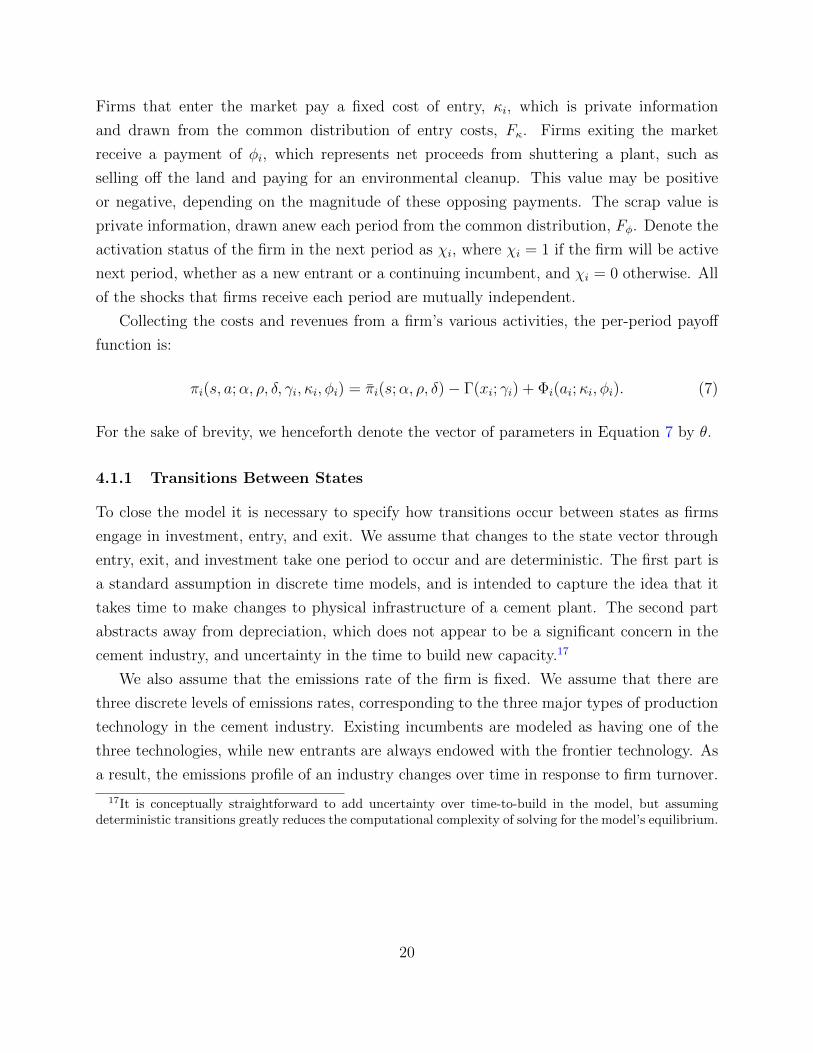
Collecting the costs and revenues from a firm’s various activities, the per-period payoff

function is:

πi(s, a;α, ρ, δ, γi, κi, φi) = π̄i(s;α, ρ, δ)− Γ(xi; γi) + Φi(ai;κi, φi). (7)

For the sake of brevity, we henceforth denote the vector of parameters in Equation 7 by θ.

4.1.1 Transitions Between States

To close the model it is necessary to specify how transitions occur between states as firms

engage in investment, entry, and exit. We assume that changes to the state vector through

entry, exit, and investment take one period to occur and are deterministic. The first part is

a standard assumption in discrete time models, and is intended to capture the idea that it

takes time to make changes to physical infrastructure of a cement plant. The second part

abstracts away from depreciation, which does not appear to be a significant concern in the

cement industry, and uncertainty in the time to build new capacity.17

We also assume that the emissions rate of the firm is fixed. We assume that there are

three discrete levels of emissions rates, corresponding to the three major types of production

technology in the cement industry. Existing incumbents are modeled as having one of the

three technologies, while new entrants are always endowed with the frontier technology. As

a result, the emissions profile of an industry changes over time in response to firm turnover.

17It is conceptually straightforward to add uncertainty over time-to-build in the model, but assumingdeterministic transitions greatly reduces the computational complexity of solving for the model’s equilibrium.

20

4.1.2 Equilibrium

In each time period, firm i makes entry, exit, production, and investment decisions, collec-

tively denoted by ai. Since the full set of dynamic Nash equilibria is unbounded and complex,

we restrict the firms’ strategies to be anonymous, symmetric, and Markovian, meaning firms

only condition on the current state vector and their private shocks when making decisions,

as in Maskin and Tirole (1988) and Ericson and Pakes (1995).

Each firm’s strategy, σi(s, εi), is a mapping from states and shocks to actions:

σi : (s, εi)→ ai, (8)

where εi represents the firm’s private information about the cost of entry, exit, investment,

and divestment. In the context of the present model, σi(s) is a set of policy functions

which describes a firm’s production, investment, entry, and exit behavior as a function of

the present state vector. In a Markovian setting, with an infinite horizon, bounded payoffs,

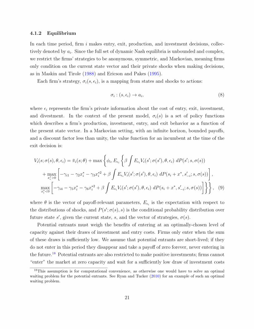
and a discount factor less than unity, the value function for an incumbent at the time of the

exit decision is:

Vi(s;σ(s), θ, εi) = π̄i(s; θ) + max

{φi, Eεi

{β

∫EεiVi(s

′;σ(s′), θ, εi) dP (s′; s, σ(s))

+ maxx∗i>0

[−γi1 − γ2x∗i − γ3x∗2i + β

∫EεiVi(s

′;σ(s′), θ, εi) dP (si + x∗, s′−i; s, σ(s))

],

maxx∗i<0

[−γi4 − γ5x∗i − γ6x∗2i + β

∫EεiVi(s

′;σ(s′), θ, εi) dP (si + x∗, s′−i; s, σ(s))

]}}, (9)

where θ is the vector of payoff-relevant parameters, Eεi is the expectation with respect to

the distributions of shocks, and P (s′;σ(s), s) is the conditional probability distribution over

future state s′, given the current state, s, and the vector of strategies, σ(s).

Potential entrants must weigh the benefits of entering at an optimally-chosen level of

capacity against their draws of investment and entry costs. Firms only enter when the sum

of these draws is sufficiently low. We assume that potential entrants are short-lived; if they

do not enter in this period they disappear and take a payoff of zero forever, never entering in

the future.18 Potential entrants are also restricted to make positive investments; firms cannot

“enter” the market at zero capacity and wait for a sufficiently low draw of investment costs

18This assumption is for computational convenience, as otherwise one would have to solve an optimalwaiting problem for the potential entrants. See Ryan and Tucker (2010) for an example of such an optimalwaiting problem.

21

before building a plant. The value function for potential entrants is:

V ei (s;σ(s), θ, εi) = max {0,

maxx∗i>0

[−γ1i − γ2x∗i − γ3x∗2i + β

∫EεiVi(s

′;σ(s′), θ, εi)dP (si + x∗, s′−i; s, σ(s))

]− κi

}. (10)

Markov perfect Nash equilibrium (MPNE) requires each firm’s strategy profile to be

optimal given the strategy profiles of its competitors:

Vi(s;σ∗i (s), σ−i(s), θ, εi) ≥ Vi(s; σ̃i(s), σ−i(s), θ, εi), (11)

for all s, εi, and all possible alternative strategies, σ̃i(s). As we work with the expected value

functions below, we note that the MPNE requirement also holds after integrating out firms’

private information: EεiVi(s;σ∗i (s), σ−i(s), θ, εi) ≥ EεiVi(s; σ̃i(s), σ−i(s), θ, εi). Doraszelski

and Satterthwaite (2010) discuss the existence of pure strategy equilibria in settings similar

to the one considered here. The introduction of private information over the discrete actions

guarantees that at least one pure strategy equilibrium exists, as the best-response curves are

continuous. However, there are no guarantees that the equilibrium is unique, a concern we

discuss next in the context of my empirical approach.

4.2 Market based emissions policy designs

We use the model to simulate both static and dynamic industry response to the introduc-

tion of both price instruments (emissions taxes) and quantity instruments (cap-and-trade

programs). In the tax regimes we consider, all domestic producers must pay τ per unit of

emissions. In the emissions trading programs we analyze, an emissions cap limits green-

house gas emissions across multiple emissions-intensive sectors. To comply with the trading

program, producers must hold permits to offset their uncontrolled emissions. We impose

no spatial or sectoral restrictions on permit trading; permits can be traded freely among

all program participants. To keep the analysis more tractable, we do not allow banking or

borrowing of permits across time.

The carbon price, τ , is an exogenous parameter. In the case of the tax, this simply means

that the level of the tax does not depend on the production and/or pollution decisions of

the regulated firms. The tax is set by the regulator and does not change over the time

horizon we consider (30 years). In the case of an emissions trading program, we assume that

the aggregate marginal abatement cost curve is flat in the neighborhood of the constraint

22

imposed by the emissions cap. This will be an appropriate assumption if the domestic

cement industry is a relatively small player in the emissions market, such that changes

in industry net supply/demand for permits cannot affect the equilibrium market price.19

The policy designs we analyze can best be classified into one of four categories: standard

auction design/ carbon tax; grandfathering (i.e. lump sum transfer); output-based rebating;

emissions-based rebating. In the subsections that follows, these policy design alternatives

are described in detail.

4.2.1 Standard design: Emissions tax or emissions trading with auctioned per-

mits

In the wake of failed attempts to implement a federal cap-and-trade program for green-

house gases, some are advocating for a reconsideration of a carbon tax.20 In the context of

an economy-wide greenhouse gas emissions trading program,a cap-and-trade program that

incorporates auctioning also has its proponents.21 Given our assumption about the exo-

geneity of the carbon price, these two market-based policy designs are, within our modeling

framework, functionally eqiuvalent.

The first policy regime we analyze is indended to capture the most salient features of

an emissions tax or an emissions cap-and-trade program in which all emissions permits are

allocated via a uniform price auction. In the tax regime, regulated firms must pay a tax τ

for each ton of emissions. In the emissions trading regime, the equilibriun permit price is τ ;

a change in the net supply or demand for permits from the domestic cement industry doesl

not affect this price.

The per-period production profit function becomes:

πit = P

(qit +

∑j 6=i

qjt;α

)qit − Ci(qit; δ)− τeiqit, (12)

19This assumption is likely to be approximately true in the context of a federal GHG trading programthat permits offsets. Keohane (2009) estimates the slope of the marginal abatement cost curve in the UnitedStates (expressed in present-value terms and in 2005 dollars) to be 8.0 x 107 $/GT CO2 for the period2010–2050. Suppose this curve can be used to crudely approximate the permit supply function. If all ofthe industries deemed to be “presumptively eligible” for allowance rebates reduced their emissions by tenpercent for this entire forty year period, the permit price would fall by approximately $0.25/ ton.

20Blinder, Alan. January 31, 2011. ”The Carbon Tax Miracle Cure”. Wall Street Journal.21 For example, in 2007, the Congressional Budget Office Director warned that a failure to auction permits

in a federal greenhouse gas emissions trading system “would represent the largest corporate welfare programthat has even been enacted in the history of the United States” ”Approaches to Reducing Carbon DioxideEmissions: Hearing before the Committee on the Budget U.S. House of Representatives”, November 1, 2007.(testimony of Peter R. Orszag)

23

where ei is the firm’s emissions rate and E represents aggregate industry emissions.

4.2.2 Grandfathering

In this policy scenario, tradable emissions permits are allocated for free to incumbent firms

that pre-date the carbon trading program. Firm-specific permit allocation schedules (i.e.

the number of permits the firm will receive each period) are determined at the beginning of

the program and are based on historic emissions.

Several studies have demonstrated that a pure grandfathering regime would grossly over-

compensate industry for the compliance costs incurred under proposed Federal climate

change legislation. For example, a recent paper finds that grandfathering fewer than 15

percent of the emissions allowances generally suffices to prevent profit losses among indus-

tries that would suffer the largest percentage losses of profit absent compensation (Goulder,

Hafstead, and Dworsky, 2010). Under the grandfathering regime we consider, we assume

that a number of permits equal to 20 percent of annual baseline emissions are grandfathered

each year to incumbent cement producers. The per period profit function becomes:

πit = P

(qit +

∑j 6=i

qjt;α

)qit − Ci(qit; δ)− τ(eiqit − Ai), (13)

with∑i

Ai = A.

The number of permits the firm receives for free from the regulator is Ai; A represents the

total amount of emissions allocated for free to domestic cement producers. We assume that

the share of emissions allowances allocated to firm i (i.e. Ai/A ) is equal to its share of the

installed kiln capacity at the outset of the program.

Note that the first order conditions associated with static profit maximization under

auctioning are identical to those under grandfathering. This highlights the so-called ”inde-

pendence property”, which holds that firms’ short run production and abatement decisions

will be unaffected by the choice between auctioning permits or allocating them freely to firms

in lump sum (Hahn and Stavins, 2010).

When permits are grandfathered in a cap and trade program, policy makers must decide

ex ante how to deal with new entrants and firms who exit. In our simulations, we assume

that a firm forfeits its future entitlements to free permits when it exits the market. We

assume that new entrants are not entitled to free permits.22 In some existing program

22In practice, policies regarding free permit allocations to free entrants and former incumbents vary. In

24

designs (including the EU ETS), some fraction of the permits to be allocated are set aside

for new production capacity entering the market. Future work will explore these alternative

policy designs that offer free permit allocations as incentive for new entrants.

4.2.3 Output-based allocation updating/rebating

The third policy regime we analyze incorporates output-based rebating. This scenario can

be motivated in two ways. First, under an emissions tax, tax revenues can be rebated to

regulated firms based on output. For example, Sweden has refunded revenues from a tax

on nitrogen oxide emissions in proportion to output (Sterner and Isaksson, 2006). Second,

our modeling approach also captures the essential features of an emissions trading program

in which free permit allocations are contingent upon production levels. For example, un-

der proposed state and federal climate change legislation, output-based updating provisions

are used to address concerns about near-term competitiveness impacts, job loss, and emis-

sions leakage. Emissions permits are allocated for free to eligible firms using a continuously

updated, output-based formula.23

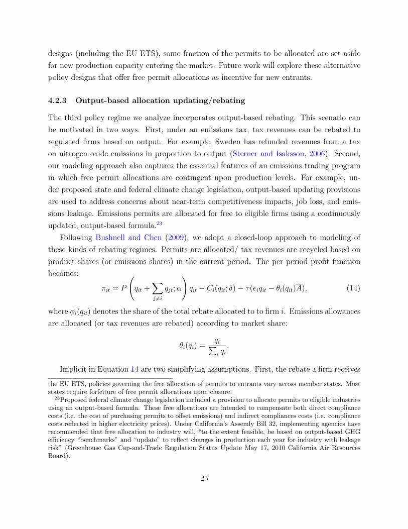
Following Bushnell and Chen (2009), we adopt a closed-loop approach to modeling of

these kinds of rebating regimes. Permits are allocated/ tax revenues are recycled based on

product shares (or emissions shares) in the current period. The per period profit function

becomes:

πit = P

(qit +

∑j 6=i

qjt;α

)qit − Ci(qit; δ)− τ(eiqit − θi(qit)A), (14)

where φi(qit) denotes the share of the total rebate allocated to to firm i. Emissions allowances

are allocated (or tax revenues are rebated) according to market share:

θi(qi) =qi∑i qi.

Implicit in Equation 14 are two simplifying assumptions. First, the rebate a firm receives

the EU ETS, policies governing the free allocation of permits to entrants vary across member states. Moststates require forfeiture of free permit allocations upon closure.

23Proposed federal climate change legislation included a provision to allocate permits to eligible industriesusing an output-based formula. These free allocations are intended to compensate both direct compliancecosts (i.e. the cost of purchasing permits to offset emissions) and indirect compliances costs (i.e. compliancecosts reflected in higher electricity prices). Under California’s Assemly Bill 32, implementing agencies haverecommended that free allocation to industry will, “to the extent feasible, be based on output-based GHGefficiency “benchmarks” and “update” to reflect changes in production each year for industry with leakagerisk” (Greenhouse Gas Cap-and-Trade Regulation Status Update May 17, 2010 California Air ResourcesBoard).

25

in the current period depends on its production level in that same period. Thus, we do not

explicitly account for the fact that firms will discount the value of the subsidy conferred by

rebating if the rebate is paid in a future period. Second, the size of the implicit subsidy

per unit of output is taken to be exogenous to firms’ production decisions. More precisely,

we assume that firms do not take into account how their production decisions affects the

size of the implicit subsidy γi via the effect on aggregate production levels. Together, these

assumptions simplify the dynamic problem considerably, while still allowing us to capture

the dynamic implications of the grandfathering mechanism to a significant extent.

4.2.4 Border tax adjustment with auctioned permits

The fourth and final policy design alternative that we consider incorporates a border tax

adjustment (BTA). The BTA mechanism imposes a carbon tax to imports, who now face the

full cost of the emissions. The idea behind the mechanism is that a carbon tax to international

firms avoids the competitiveness wedge between domestic firms and their foreign competitors.

In the case that we consider, domestic firms do not receive any free allowance and there-

fore the mechanism is equivalent to auctioning in terms of strategic incentives. However,

they face a different residual demand, as the import supply is shifted to the left as follows:

lnMm = ρ0 + ρ1 ln(Pm − τem), (15)

where em is the emissions rates on imported cement.

4.3 Modeling Emissions Abatement

Section 3.1 included a discussion of how carbon dioxide emissions reductions can be achieved

in the domestic cement industry. If emissions from cement manufacturing were to be subject

to a binding cap, it is anticipated that mandated emissions reductions would be achieved

through a combination of factors. Chief among these are the replacement of old production

processes with new state-of-the-art technology and the increased substitution of less carbon

intensive materials for clinker or cement.

We explicitly model what is expected to be the most important efficiency improvement:

the replacement of older kiln technology with current, state-of-the-art technology. Our mod-

eling approach is well suited to modeling the retirement of old process equipment and entry

of new firms. We assume all new entrants adopt new, state-of-the-art equipment. This as-

sumption finds empirical support in the data. Our specific assumptions about the emissions

26

intensities of old and new production equipment are described in Appendix A.

The substitution of SCM for clinker is also expected to play an important role in delivering

emissions reductions in a carbon constrained cement industry. Supplementary cementitious

materials are used widely throughout the U.S. as additives to concrete. Utilization rates

have varied due to economic considerations and the availability of materials. Although we

do not explicitly model the substitution of SCMs for clinker, this substitution is implicitly

captured, to some extent, by our estimated demand elasticity.

Ideally, a model designed to simulate industry response to an emissions regulation would

accurately capture all viable carbon abatement strategies. Unfortunately, our econometric

approach is not well suited to modeling responses that have yet to be observed in the data.

Consequently, fuel switching and carbon sequestration are not represented in our model. Al-

though these options are not expected to play as significant a role as efficiency improvements

or substitution, this omission will bias up our estimates of the economic costs imposed of

the emissions regulations we analyze.24

5 Estimation and computation

The econometric estimation is based on the benchmark model, in which the price of emissions

is set to zero (τ = 0), i.e. there is no compliance cost due to emissions regulation. Once

estimated, this model can be used to simulate the dynamic industry response to market-

based emissions regulations that affect firms’ production and investment choices primarily

through operating costs provided certain assumptions are met. In particular, we will assume

that firms’ response to a given operating cost change is independent of whether the cost

change is caused by emissions regulation or other exogenous factors (such as changes in

energy prices or other inputs).

5.1 Estimation

Although our data sources and identification strategy are similar to Ryan (2011), there are

some important differences in how the model is specified and estimated. In this section,

significant deviations are discussed. The interested reader is referred to Ryan (2011) for

additional details regarding the data and estimation.

24In future work we plan to compute what would be an upper bound on the cost of fuel switching for itto be observed in equilibrium together with sensitivity analysis on how important such adoption would befor mitigating the adverse effects of carbon regulation.

27

Table 1: Descriptive Statistics for Regional Markets (based on 2006 data)

Market Number of Firms Capacity Emissions Rate Import Market Share

Atlanta 6 1285 0.97 0.12Baltimore/Philadelphia 6 1497 0.99 0.12Birmingham 5 1288 0.94 0.35Chicago 5 972 0.98 0.04Cincinnati 3 875 0.93 0.21Dallas 5 1766 1.05 0Denver 4 998 0.95 0Detroit 3 1749 1.02 0.19Florida 5 1297 0.93 0.35Kansas City 4 1661 0.95 0Los Angeles 6 1733 0.93 0.18Minneapolis 1 1862 0.93 0.2New York/Boston 4 1033 1.16 0.45Phoenix 4 1138 0.93 0.13Pittsburgh 3 614 1.08 0Salt Lake City 2 1336 1.01 0San Antonio 6 1318 0.95 0.3San Francisco 4 931 0.93 0.18Seattle 2 607 1.05 0.65St Louis 4 1358 1.05 0

5.1.1 Regional market definition

The USGS collects establishment-level data from all domestic Portland cement producers

and publishes these data in an annual Minerals Yearbook. Cement price and sales data are

aggregated to the regional market level to protect the confidentiality of the respondents. In

recent years, increased consolidation of asset ownership has required higher levels of data

aggregation. Conversations with the experts at USGS indicate that the current regional

market definitions group plants that are unlikely to compete with each other (Van Oss,

personal communication).

Rather than adopt the USGS protocols, we base our regional market definitions on the

industry-accepted limitations of economic transport as well as company-specific SEC 10k

filings which include information regarding markets served by specific plants. To merge the

USGS cement prices with our data set, USGS prices are weighted by kiln capacity in each

region. For example, if kiln capacity in the region we define as region A is equally divided

between USGS defined markets B and C, we define the price in region A to be the average

price reported in USGS markets B and C. We report some descriptive statistics using USGS

data from 2006 for our regional markets in Table 1.

This table helps to highlight inter-regional variation in market size, emissions intensity,

and trade exposure. Notably, the degree of import penetration varies significantly across

28

inland and coastal areas. Whereas several inland markets are supplied exclusively by do-

mestic production, imports now account for over half of domestic cement consumption in

Seattle.Import penetration rates tend to be highest along the coasts versus inland waterways.

In our analysis, we will be interested in understanding how policy responses differ across

regional markets that differ in terms of trade exposure, concentration of ownership, etc.

However, data limitations prevent us from estimating market specific demand and cost pa-

rameters. For example, we will use the same average demand elasticity parameter in all

regional market simulations. These average demand parameter values may overstate the

residual demand faced by firms in some markets. This can trigger immediate investment

in some markets, particularly those that are spatially sparse. To deal with this problem,

we first simulate outcomes in each regional market with no carbon policy in place for one

period so that investments can adjust if needed. Once these investments have been made,

we introduce the carbon policy. This approach is intended to separate the effects of possible

misspecification in the model or demand estimation from the effects of the counterfactual

policy on simulated outcomes. 25

5.1.2 Import supply and residual demand elasticities

We estimate the following demand equation using two stage least squares (2SLS):

lnQmt = γ0 + γ1 lnPmt + γ2m + γ′3 lnXmt + ε1mt. (16)

The dependent variable is the natural log of the total market demand in market m in

year t. The coefficient on market price, γ1, is the elasticity of demand, and Xmt is a set of

demand shifters.

We instrument for the potential endogeneity of cement price using supplyside cost shifters:

coal prices, gas prices, electricity rates, and wage rates. Each market has a demand shifter

in the intercept, γ2m, using Atlanta as the baseline market. Data sources are summarized in

Ryan (2011).

Given our interest in understanding how policy-induced operating cost increases could

affect import penetration rates, it will be important to separate the import supply response

to changes in domestic operating costs from the domestic market demand response. We

estimate the following import supply schedule using 2SLS:

25Runningthe model without this adjustment generates similar qualitative results, although the negativewelfare effects from cap-and-trade are exacerbated in the non-adjusted model.

29

lnMmt = φ0 + φ1 lnPmt + φ2m + φ′3 lnZmt + ε2mt. (17)

This model is estimated using data from those markets exposed to import competition

over the period 1993-2007. For inland markets supplied entirely by domestic production, all

φ coefficients are set to zero. The dependent variable is the log of the quantity of cement

shipped to market m in year t. The average customs price of cement is Pmt. These data are

collected by the U.S. Geological Survey and are published in the annual Minerals Yearbook.

These data are reported by Customs districts (i.e. groupings of ports of entry). These

districts are matched to the regional markets described in the previous section.

We instrument for the import price using new residential construction building starts,

gross state product, value of construction, and population. These state-level data are ag-

gregated for all states included in the regional market area. The matrix Zmt includes other

plausibly exogenous factors that affect import supply. To capture transportation costs, we

subtract the average customs price from the average C.I.F. price of the cement shipments.

This residual price accounts for the transportation cost on a per unit basis, as well as the

insurance cost and other shipment-related charges. The Zmt matrix also includes coal and

oil prices to capture variation in production costs. Region dummy variables capture regional

differences.

To construct the residual demand curve faced by domestic producers in a trade exposed

market, the import supply at a given price is subtracted from the aggregate demand at that

price. The resulting residual demand does not necessarily feature a constant elasticity and

potentially features a kink at the price below which importers do not supply any output

at the market. In practice, in all the counterfactual simulations some positive imports are

observed at coastal markets.26

5.2 Estimation results

Table 2 enumerates the parameter estimates used in our simulations. Overall, these estimates

appear reasonable.

• The marginal cost estimate of $30/ton of clinker falls well within the range that is

typically reported for domestic production: $27-$44 per ton (Van Oss, 2003 ENV).

26This is intuitive as the costs of the domestic industry increase in the counterfactuals considered, whichweakly raises the market price.

30

• The import supply elasticity point estimate is 2.5. When analyzing the impacts of

environmental regulations, the US EPA assumes an import supply elasticity of 2 for

the cement sector based on Broda et al (2008).

• The elasticity of aggregate demand is 2.96. This is higher in absolute value than some

other demand elasticities reported in the literature. For example, Jans and Rosenbaum

(1996) estimate a domestic demand elasticity of -0.81. On the other hand, using much

higher-quality data, Foster, Haltiwanger, and Syverson (2008) estimate several similar

high demand elasticities for homogeneous goods industries, such as −5.93 for ready-

mixed concrete, cement’s downstream industry.

• Investment costs are roughly in line with the accounting costs cited in Salvo (2010),

which reports a cost of $200 per ton of installed capacity. Our numbers are slightly

higher, which in line with the idea that these costs represent economic opportunity

costs as opposed to accounting costs. The implied cost of a cement plant is also in line

with plant costs reported in newspapers and trade journals. For example, on October

15, 2010, it was reported that the most recent expansion of the Texas Industries New

Braunfels cement plant, increasing capacity from 900 thousand tons per year to 2.3

million tons per year, was pegged at a cost of $350M, which implies a cost of $250 per

ton of installed capacity.27

• The magnitudes of the fixed costs are reasonable at face value, and in conjunction with

the estimated variances, are in accord with the observed rates of investment, entry, and

exit in the cement industry.

Some of the parameters from the model described above are not reported. Substantial

divestment is virtually never observed in the data and thus the estimates of divestment costs

to be very large. Fixed costs of production and operation are also not reported, as these

are set to zero. The reason is that we do not observe sufficient periods of operation without

production (mothballing) which are required to separately identify those parameters from

the distribution of exit costs.

5.3 Computation

Once the parameters have been estimated, the model can be computed to compare the market

performance under market-based policy designs. In order to compute the equilibrium of the

27Source: KGNB Radio, New Braunfels, Texas.

31

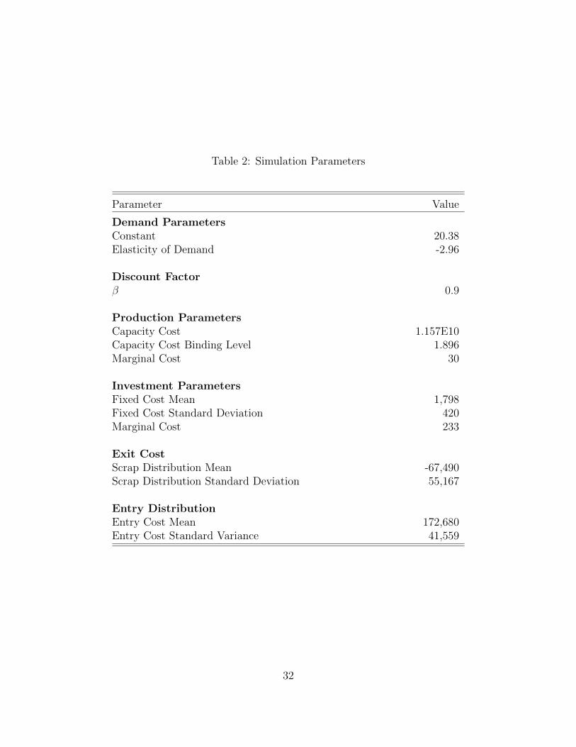
Table 2: Simulation Parameters

Parameter Value

Demand ParametersConstant 20.38Elasticity of Demand -2.96

Discount Factorβ 0.9

Production ParametersCapacity Cost 1.157E10Capacity Cost Binding Level 1.896Marginal Cost 30

Investment ParametersFixed Cost Mean 1,798Fixed Cost Standard Deviation 420Marginal Cost 233

Exit CostScrap Distribution Mean -67,490Scrap Distribution Standard Deviation 55,167

Entry DistributionEntry Cost Mean 172,680Entry Cost Standard Variance 41,559

32

game, we make use of parametric approximation methods. In particular, we interpolate

the value function using cubic splines. The reasons behind using parametric methods are

twofold. First, the game has a continuous state space, given by the vector of capacities of

the firms. By using parametric methods, we can allow firms to deterministically choose their

capacity in a continuous space. Second, parametric approximation methods can be useful to

improve computational speed. Previous work has already suggested the potential benefits of

using parametric approximation methods (Pakes and McGuire, 1994).

Parametric value function methods have been explored in a single agent dynamic pro-

gramming context.28 However, they have not been widely used in dynamic games, particu-

larly in games in which players take discrete actions, such as entry and exit (Doraszelski and

Pakes, 2007). In our application, we find the method to perform well compared to a discrete

value function method. In particular, this parametric method allows us to treat capacity as

a continuous state, which improves the convergence properties of the game.29

The procedure we use is similar in spirit to the discrete value function iteration ap-

proach. In both methods, the value function is evaluated at a finite number of points. At

each iteration and for a given guess of the value function, firms’ strategies are computed op-

timally (policy step). Then, the value function is updated accordingly (value function step).

This process is repeated until the value function and the policy functions do not change

significantly.

The difference between the discrete value function iteration and our iterative approach is

that we approximate the value function with a flexible parametric form. In particular, given

a guess for the value function V k at pre-specified grid points, we interpolate the value func-

tion with a multi-dimensional uniform cubic spline, which can be computed very efficiently

(Habermann and Kindermann, 2007).30 This interpolation defines an approximation of the

value function in a continuous space of dimension equal to the number of active firms. For

a given number of firms active NA in the market, the value function at any capacity vector

s is approximated as,

V̂ ki (s) =

(J+2)A∑j=1

φNA,jBNA,j(s), (18)

28For a general treatment of approximation methods used in the context of dynamic programming, seeJudd (1998). An assessment of these methods in a single agent model can be found in Benitez-Silva et al.(2000).

29This is mainly driven by the fact that firms take deterministic actions with respect to the continuousstate.

30For a detailed treatment of splines methods, see de Boor (2001).

33

where J is the number of grid points, φNA,ij are the coefficients computed by interpolating

the values V k when there are A active firms, and BNA,j(s) is the spline weight given to

coefficient φNA,j when the capacity state equals s. This coefficient is the product of capacity

weights for each of the incumbent firms, so that BNA,j(s) =∏

i∈ABj(si).

In the policy step, optimal strategies are computed over this continuous function. For a

given firm, we compute the conditional single-dimensional value function, given the capacity

values of the other firms, V̂ ki (si|s−i). This formulation allows us to represent the single-

dimensional investment problem of the firm. The following expression defines the expected

value function of the firm conditional on staying in the market and investing to a new capacity

s′i. Firms maximize,

maxs′i

πi(si, s′i|s−i) +

∑s′−i∈S−i

Prk(s′−i;σk(s))V̂ k

i (s′i|s′−i). (19)

We compute the optimal strategy by making use of the differentiability properties of

the cubic splines, which allows us to compute the first-order conditions with respect to

investment. Given that the cubic spline does not restrict the value function to be concave,

we check all local optima in order to determine the optimal strategy of the firm.31 Conditional

on optimal investment strategies, we then compute the new policy function with respect to

the entry, investment and exit probabilities, which gives us an updated optimal policy σk+1.

This allows us to compute a new guess for the value function V k+1 in the value function step.

The process is iterated until the strategies for each of the firms and the value function

in each of the possible states do not change more than an established convergence criterion,

such that ‖ σk+1 − σk ‖< εσ and ‖ V k+1 − V k ‖< εV .

6 Welfare measures and metrics

In this section, we first describe the analytical framework we will use to interpret the results.

We then discuss an important parameter in our analysis: the social cost of carbon.

31Given that the cubic spline is defined by a cubic polynomial at each of the grid intervals, this impliesthat at most there will be 2(J − 1) + 2 candidate local optima, where J is the number of grid points.

34

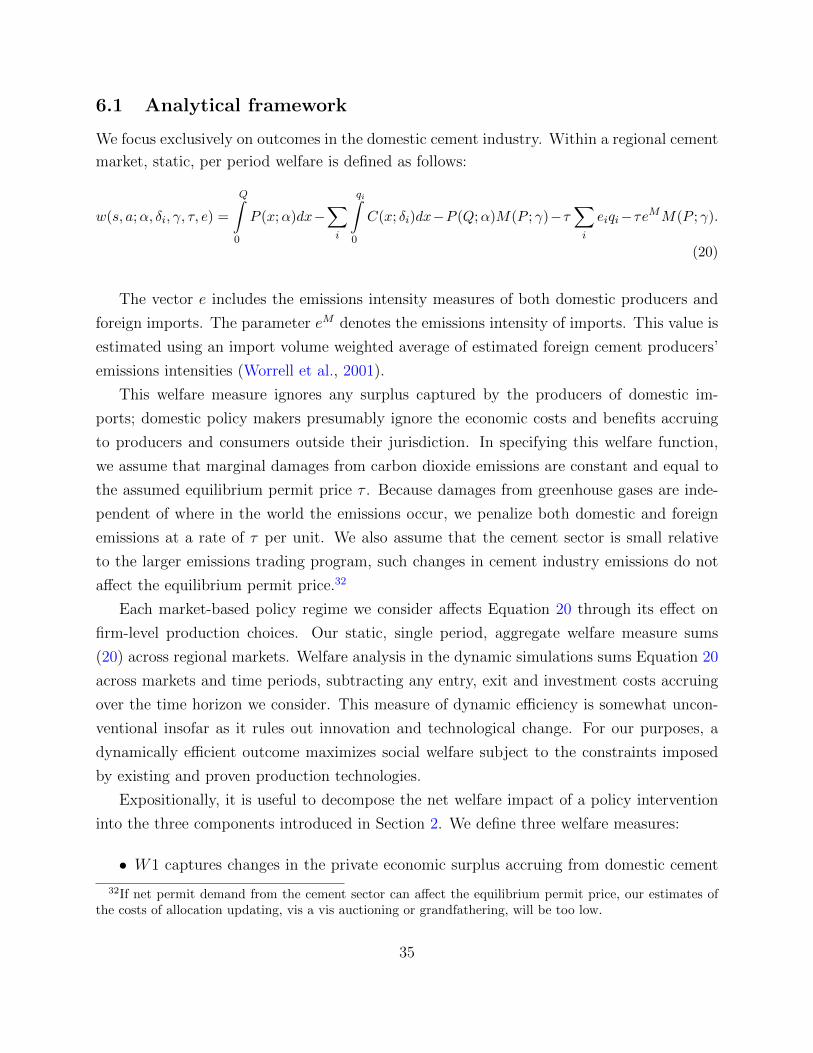
6.1 Analytical framework

We focus exclusively on outcomes in the domestic cement industry. Within a regional cement

market, static, per period welfare is defined as follows:

w(s, a;α, δi, γ, τ, e) =

Q∫0

P (x;α)dx−∑i

qi∫0

C(x; δi)dx−P (Q;α)M(P ; γ)−τ∑i

eiqi−τeMM(P ; γ).

(20)

The vector e includes the emissions intensity measures of both domestic producers and

foreign imports. The parameter eM denotes the emissions intensity of imports. This value is

estimated using an import volume weighted average of estimated foreign cement producers’

emissions intensities (Worrell et al., 2001).

This welfare measure ignores any surplus captured by the producers of domestic im-

ports; domestic policy makers presumably ignore the economic costs and benefits accruing

to producers and consumers outside their jurisdiction. In specifying this welfare function,

we assume that marginal damages from carbon dioxide emissions are constant and equal to

the assumed equilibrium permit price τ . Because damages from greenhouse gases are inde-

pendent of where in the world the emissions occur, we penalize both domestic and foreign

emissions at a rate of τ per unit. We also assume that the cement sector is small relative

to the larger emissions trading program, such changes in cement industry emissions do not

affect the equilibrium permit price.32

Each market-based policy regime we consider affects Equation 20 through its effect on

firm-level production choices. Our static, single period, aggregate welfare measure sums

(20) across regional markets. Welfare analysis in the dynamic simulations sums Equation 20

across markets and time periods, subtracting any entry, exit and investment costs accruing

over the time horizon we consider. This measure of dynamic efficiency is somewhat uncon-

ventional insofar as it rules out innovation and technological change. For our purposes, a

dynamically efficient outcome maximizes social welfare subject to the constraints imposed

by existing and proven production technologies.

Expositionally, it is useful to decompose the net welfare impact of a policy intervention

into the three components introduced in Section 2. We define three welfare measures:

• W1 captures changes in the private economic surplus accruing from domestic cement

32If net permit demand from the cement sector can affect the equilibrium permit price, our estimates ofthe costs of allocation updating, vis a vis auctioning or grandfathering, will be too low.

35

consumption (i.e. the first three terms in Equation 20.

• W2 accounts for both economic surplus changes (W1) plus the benefits of emissions

reductions.

• W3 accounts for emissions leakage across policy designs by penalizing foreign increases

in emissions.

In this preliminary draft, we report results from simulating outcomes in twelve out of

twenty regional markets: Cincinnati, Denver, Detroit, Kansas City, Minneapolis, New York,

Phoenix, Pittsburgh, Salt Lake City, San Francisco, Seattle, and St. Louis. Across re-

gional markets we analyze, there is significant variation in market size, plant technology,

and import presence. For example, the Salt Lake City market is not accessible by water

and demand is met entirely by domestic suppliers, who have heterogeneity in their emissions

rates. In contrast, a market like San Francisco is trade-exposed and incumbent producers

are homogeneous with respect to emissions rates.

In the future, the scope of the analysis will be expanded to include all domestic cement

markets. This will allow us to provide a more comprehensive assessment of the industry-

wide effects of the policies we consider, and to assess the extent to which a “one-size-fits-all”

policy regime can result in differential outcomes across heterogeneous regional markets.

6.2 The Social Cost of Carbon

The τ value we use to penalize each ton of simulated CO2 emissions is intended to capture the

monetized damages associated with an incremental (one ton) increase in carbon emissions.

Given the uncertainty inherent in this kind of policy analysis, it is important to consider a

range of values of τ . The range of values we choose to consider, $5 to $65 per ton of CO2,

is informed by a landmark interagency process which produced estimates of the social cost

of carbon (SCC) for use in policy analysis(Greenstone et al., 2011).

Table 3 summarizes the four SCC schedules that were selected in this process. In light

of disagreements about the appropriate choice of interest rate, three different discount rates

are used (corresponding to the first three schedules). The final schedule (fourth column)

corresponds to a scenario with higher than expected economic costs from climate change. The

SCC increases over time because future emissions are expected to produce larger incremental

damages as physical and economic systems become more stressed.33

33In our analysis, we assume the carbon price does not change over the time horizon we consider.

36

Table 3: Estimated social cost of carbon($ per metric ton of carbon dioxide in $2007)

(1) (2) (3) (4)

Discount rate 5% 3% 2.5% 3%

2010 4.70 21.40 35.10 64.90

2020 6.80 26.30 41.70 80.70

2030 9.70 32.80 50.00 100.00

Source: U.S. Department of Energy (2010), “Final Rule Technical Support Document (TSD):Energy Efficiency Program for Commercial and Industrial Equipment: Small Electric Motors,”Appendix 15A (by the Interagency Working Group on Social Cost of Carbon): “Social Cost ofCarbon for Regulatory Impact Analysis Under Executive Order 12866”.

Another important assumption we make is that the carbon price reflects the true social

cost of carbon. Thus, the carbon tax or permit price and the social cost of carbon are

assumed to be one and the same. This approach has expositional advantages. However, it

is essential to keep this assumption in mind when comparing results across scenarios. An

alternative approach would hold the assumed SCC value constant across scenarios associated

with different permit prices/tax levels, which we discuss below.

7 Simulation results

Before turning to the simulation results, it is important to highlight some underlying as-

sumptions and to issue some caveats with respect to interpretation.

One assumption underpinning our counterfactual simulations is that cement producers

will respond to economic changes induced by a market-based emissions regulation in the same

way that they have responded historically to similar changes induced by other exogenous

market forces. This assumption seems quite plausible given that the policy designs we

consider operate solely through altering production costs and revenues.

Another important assumption is that our structural assumptions, including assumptions

about how firms respond to changes in policy incentives, will hold out of sample. We observe

significant variation in plausibly exogenous supply and demand shifters across regional mar-

37

kets and across time; this variation is essential to identification. However, our inferences at

high carbon prices are quite far from historical experience. To put this in context, consider

that a carbon price of $60/ton would approximately triple the estimated marginal operating

costs of the average cement producer. A higher-level concern is that plausible general equi-

librium effects of high carbon prices could lead to unforeseen structural shifts in the supply

and demand curves characterizing cement outcomes.

In what follows, we have elected to report simulation results for the range of SCC values

that have been deemed policy relevant. However, it is important to keep in mind that the

higher the carbon price we consider, the farther out counterfactual is from the data we

observe, and the more sensitive our simulation results will be to our modeling assumptions.

That said, we believe that our results both help illustrate the general forces shaping the

interaction of market structure and carbon regulation and provide the best possible estimates

of efficiency and distributional welfare effects under a range of policies.

This section begins with a summary of the simulated static and dynamic responses of the

domestic cement industry to the range of counterfactual policy interventions we consider.

We begin by emphasizing the results using the model that accounts for industry dynamics.

We then contrast our welfare measures across the static and dynamic simulation exercises.

We conclude with a discussion of how outcomes vary across regional markets with different

characteristics.

7.1 Market outcomes and aggregate welfare measures

7.1.1 Cement prices

Figure 3 plots quantity-weighted average cement prices as a function of the exogenous permit

price (or emissions tax) τ . The introduction of market-based emissions regulation increases

equilibrium cement prices across the range of τ values we consider. Cement price increases

are most pronounced under the BTA and standard auction/tax regime. Under this policy

design, firms must bear the complete cost of compliance; no compensation in the form of

contingent rebates or lump sum transfers is offered. The prices are highest in the case of

BTA, given that both domestic and international firms face the full cost of the emissions.

Note that equilibrium cement prices vary across grandfathering and auctioning regimes.

Thus, the so-called independence property fails to hold when industry dynamics are incorpo-

rated into the model. Under the grandfathering regime, an incumbent firm receives a lump

sum transfer each period in the form of free permit allocation. An incumbent firm forfeits

38

Figure 3: Counterfactual: Cement Prices

6070

8090

100

110

Cem

ent p

rice

($/to

n)

0 20 40 60CO2 price ($/ton)

Auctioning (Dynamic) Grandfathering (Dynamic)Output (Dynamic) BTA (Dynamic)

this entitlement when it chooses to exit. This lowers the exit threshold for incumbents such

that exit rates are lower under grandfathering as compared to auctioning. As a consequence,

cement markets are less concentrated at higher permit prices, and equilibrium cement prices

are lower compared to the standard auctioning/emissions tax case.

A striking feature of Figure 3 is that, for a given value of τ , cement prices are much lower

under the policy regime that incorporates dynamic rebating. The production subsidy that

is implicitly conferred by rebating partially mitigates the impact of the emissions regulation

on cement prices.

7.1.2 Industry profits

Figure 4 plots the present discounted profits earned by the regulated domestic cement pro-

ducers over the range of carbon values we consider. For any given value of τ , profits are

most significantly impacted by the auctioning regime because firms must pay the tax (or

hold permits) to offset emissions, but receive no rebate or compensation for incurring these

costs. It is notable that the BTA scheme partially compensates firms by mitigating the role

of international competition.

Note that discounted industry profits are increasing with τ over the range of higher carbon

39

Figure 4: Counterfactual: Cement Profits

010

000

2000

030

000

4000

0F

irm p

rofit

s ($

M)

0 20 40 60CO2 price ($/ton)

Auctioning (Dynamic) Grandfathering (Dynamic)Output (Dynamic) BTA (Dynamic)

values in the grandfathering regime. As the carbon price increases, so does the value of the

lump sum transfer (in the form of free permits) allocated to incumbent firms. At very high

permit prices, some firms will have an incentive to sell permits versus using them to offset

their own emissions. This revenue from selling unused permits explains the non-monotonic

and increasing (in τ) discrepancy in profits across rebating and grandfathering regimes.

7.1.3 Domestic emissions

Policy makers are very concerned about how industry emissions will be impacted by al-

ternative forms of market-based emissions regulation. Figure 5 shows how emissions from

domestic cement producers, summed across all markets and time periods, decreases with τ .

For a given carbon price, the net cost of emitting carbon dioxide (as perceived by firms),

is highest under the auctioning regime and lowest under contingent rebating. Consequently,

industry emissions are lowest under the auctioning regime and highest under the rebating

regime. Whereas firms perceive the same costs of emissions under BTA and auctioning,

domestic emissions are higher under BTA due to the smaller competition. However, overall

emission reductions are largest under BTA.

40

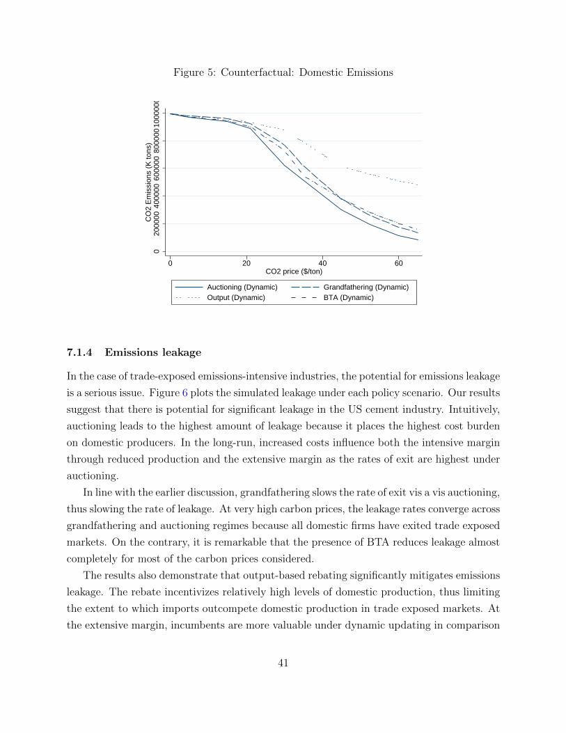
Figure 5: Counterfactual: Domestic Emissions

020

0000

4000

0060

0000

8000

0010

0000

0C

O2

Em

issi

ons

(K to

ns)

0 20 40 60CO2 price ($/ton)

Auctioning (Dynamic) Grandfathering (Dynamic)Output (Dynamic) BTA (Dynamic)

7.1.4 Emissions leakage

In the case of trade-exposed emissions-intensive industries, the potential for emissions leakage

is a serious issue. Figure 6 plots the simulated leakage under each policy scenario. Our results

suggest that there is potential for significant leakage in the US cement industry. Intuitively,

auctioning leads to the highest amount of leakage because it places the highest cost burden

on domestic producers. In the long-run, increased costs influence both the intensive margin

through reduced production and the extensive margin as the rates of exit are highest under

auctioning.

In line with the earlier discussion, grandfathering slows the rate of exit vis a vis auctioning,

thus slowing the rate of leakage. At very high carbon prices, the leakage rates converge across

grandfathering and auctioning regimes because all domestic firms have exited trade exposed

markets. On the contrary, it is remarkable that the presence of BTA reduces leakage almost

completely for most of the carbon prices considered.

The results also demonstrate that output-based rebating significantly mitigates emissions

leakage. The rebate incentivizes relatively high levels of domestic production, thus limiting

the extent to which imports outcompete domestic production in trade exposed markets. At

the extensive margin, incumbents are more valuable under dynamic updating in comparison

41

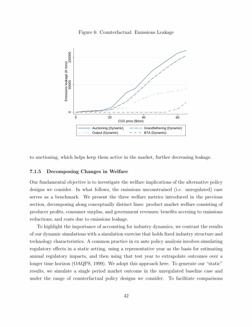
Figure 6: Counterfactual: Emissions Leakage

050

000

1000

00E

mis

sion

s le

akag

e (K

tons

)

0 20 40 60CO2 price ($/ton)

Auctioning (Dynamic) Grandfathering (Dynamic)Output (Dynamic) BTA (Dynamic)

to auctioning, which helps keep them active in the market, further decreasing leakage.

7.1.5 Decomposing Changes in Welfare

Our fundamental objective is to investigate the welfare implications of the alternative policy

designs we consider. In what follows, the emissions unconstrained (i.e. unregulated) case

serves as a benchmark. We present the three welfare metrics introduced in the previous

section, decomposing along conceptually distinct lines: product market welfare consisting of

producer profits, consumer surplus, and government revenues; benefits accruing to emissions

reductions; and costs due to emissions leakage.

To highlight the importance of accounting for industry dynamics, we contrast the results

of our dynamic simulations with a simulation exercise that holds fixed industry structure and

technology characteristics. A common practice in ex ante policy analysis involves simulating

regulatory effects in a static setting, using a representative year as the basis for estimating

annual regulatory impacts, and then using that test year to extrapolate outcomes over a

longer time horizon (OAQPS, 1999). We adopt this approach here. To generate our “static”

results, we simulate a single period market outcome in the unregulated baseline case and

under the range of counterfactual policy designs we consider. To facilitate comparisons

42

Figure 7: Counterfactual: W1

−50

000−

4000

0−30

000−

2000

0−10

000

0E

cono

mic

sur

plus

cha

nge

(mill

ions

of d

olla

rs)

0 20 40 60CO2 price ($/ton)

Auctioning (Dynamic) Grandfathering (Dynamic)Output (Dynamic) BTA (Dynamic)Auctioning (Static) Grandfathering (Static)Output (Static) BTA (Static)

with our dynamic simulations, these results are expressed as net present values using a

social discount rate of three percent. We assume the simulated annual outcomes would be

observed each year of the 30 year time horizon we consider.

W1: Product Market Surplus Changes in the first welfare metric, W1, capture dif-

ferences in producer and consumer surplus while also accounting for revenues raised by the

government through taxation or permit sales. This is a measure of how the local market

changes in response to the regulation, and is a major component of understanding welfare

changes in concentrated industries.

Figure 7 shows how economic surplus is impacted across policy designs and assumed

carbon prices. Given that this W1 measure captures none of the benefits from emissions

abatement, these changes are all negative.

An interesting result to emerge from the static simulations (in red) is the lack of industry

response to carbon prices at or below $20. In the benchmark (unregulated) case, many firms

are capacity constrained, producing at a corner solution, and thus are earning scarcity rents.

When firms are required to internalize a relatively low emissions cost at a per unit cost of

$20 or less, scarcity rents are reduced, but output decisions are essentially unaffected in the

short run.

43

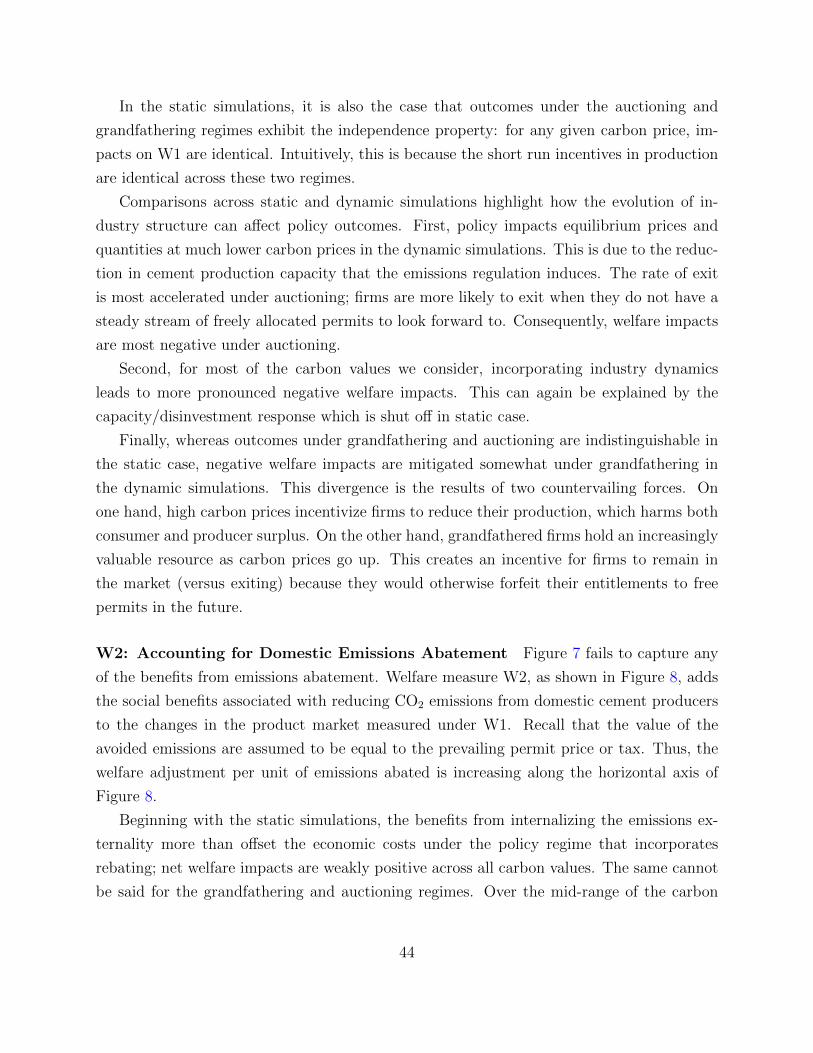
In the static simulations, it is also the case that outcomes under the auctioning and

grandfathering regimes exhibit the independence property: for any given carbon price, im-

pacts on W1 are identical. Intuitively, this is because the short run incentives in production

are identical across these two regimes.

Comparisons across static and dynamic simulations highlight how the evolution of in-

dustry structure can affect policy outcomes. First, policy impacts equilibrium prices and

quantities at much lower carbon prices in the dynamic simulations. This is due to the reduc-

tion in cement production capacity that the emissions regulation induces. The rate of exit

is most accelerated under auctioning; firms are more likely to exit when they do not have a

steady stream of freely allocated permits to look forward to. Consequently, welfare impacts

are most negative under auctioning.

Second, for most of the carbon values we consider, incorporating industry dynamics

leads to more pronounced negative welfare impacts. This can again be explained by the

capacity/disinvestment response which is shut off in static case.

Finally, whereas outcomes under grandfathering and auctioning are indistinguishable in

the static case, negative welfare impacts are mitigated somewhat under grandfathering in

the dynamic simulations. This divergence is the results of two countervailing forces. On

one hand, high carbon prices incentivize firms to reduce their production, which harms both

consumer and producer surplus. On the other hand, grandfathered firms hold an increasingly

valuable resource as carbon prices go up. This creates an incentive for firms to remain in

the market (versus exiting) because they would otherwise forfeit their entitlements to free

permits in the future.

W2: Accounting for Domestic Emissions Abatement Figure 7 fails to capture any

of the benefits from emissions abatement. Welfare measure W2, as shown in Figure 8, adds

the social benefits associated with reducing CO2 emissions from domestic cement producers

to the changes in the product market measured under W1. Recall that the value of the

avoided emissions are assumed to be equal to the prevailing permit price or tax. Thus, the

welfare adjustment per unit of emissions abated is increasing along the horizontal axis of

Figure 8.

Beginning with the static simulations, the benefits from internalizing the emissions ex-

ternality more than offset the economic costs under the policy regime that incorporates

rebating; net welfare impacts are weakly positive across all carbon values. The same cannot

be said for the grandfathering and auctioning regimes. Over the mid-range of the carbon

44

Figure 8: Counterfactual: W2

−50

000

5000

1000

015

000

Wel

fare

cha

nge

(mill

ions

of d

olla

rs)

0 20 40 60CO2 price ($/ton)

Auctioning (Dynamic) Grandfathering (Dynamic)Output (Dynamic) BTA (Dynamic)Auctioning (Static) Grandfathering (Static)Output (Static) BTA (Static)

values we consider, the net welfare impacts are negative. This result is driven by Buchanan’s

observation that there are two competing distortions in concentrated markets with externali-

ties. As the assumed social cost of carbon increases, the value of avoided damages ultimately

overwhelms the value of the lost economic surplus, and the net welfare impacts turn positive.

The dynamic simulations yield somewhat different results. Welfare gains associated with

rebating regimes and grandfathering in the dynamic case are larger than those generated

using the static model. This is partly due to firms’ ability to invest in cleaner produc-

tion equipment (which reduces the emissions intensity per unit of cement produced) and

partly because the quantity produced is lower, resulting in lower damages from domestic

emissions. The factors that made auctioning and grandfathering unattractive under metric

W1—namely, output contraction and the accelerated exit of domestic producers—make them

attractive under metric W2 once we account for the benefit of carbon emissions reductions.

W3: Accounting for Emissions Leakage Carbon dioxide is a global, uniformly mixed

pollutant. A comprehensive welfare analysis of policy impacts should account for any policy-

induced increases in emissions in other jurisdictions. Our final welfare metric, W3, augments

W2 by accounting for damages associated with emissions leakage. Emissions occurring in

45

Figure 9: Counterfactual: W3

−50

000

5000

1000

0W

elfa

re c

hang

e (m

illio

ns o

f dol

lars

)

0 20 40 60CO2 price ($/ton)

Auctioning (Dynamic) Grandfathering (Dynamic)Output (Dynamic) BTA (Dynamic)Auctioning (Static) Grandfathering (Static)Output (Static) BTA (Static)

other jurisdictions are penalized at the same rate as domestic emissions.34

Figure 9 illustrates the welfare impacts of the policy regimes we consider using this more

comprehensive welfare measure. In the static simulations, once leakage is accounted for, wel-

fare impacts of the grandfathering and auctioning regimes are negative across the full range

of carbon values we consider. In contrast, the benefits from domestic emissions reductions

more than offset costs associated with emissions leakage and the excessive withholding of

output and investment in the upper range of carbon values when rebates are incorporated

in the policy design.

In the dynamic simulations, the net welfare impacts remain at or close to zero for all

carbon values below $35. Net welfare impacts of grandfathering and auctioning are negative

for carbon values below $50. The welfare ordering of policy regimes no longer reverses at

higher carbon values. The policy designs that incorporate rebating welfare dominate over

most of the range of carbon values we consider.

The benefits from the BTA mechanism come clear under welfare measure W3. Differences

in leakage between the BTA and the auctioning mechanism increase the wedge between the

two mechanism, making the BTA mechanism more attractive. For the highest carbon price

34Ignoring co-pollutants, damages from emissions are independent of location. This contrasts to otheremissions that have spatially-varying damages. See, for example, Fowlie and Muller (2010).

46

Table 4: Dynamic simulation results: Social cost of carbon values $21 and $35/ton CO22

Outcome SCC Base- Auction Grand- Output- BTAValue line father updating

Market size 21 58,831.79 52,120.92 54,209.55 54,821.92 52,989.76(tons per year) 35 58,831.79 37,546.95 52,116.94 47,351.27 39,538.35

Q. weighted price 21 63.69 65.95 65.23 65.00 66.86($/ton) 35 63.69 75.17 72.02 67.81 77.45

Domestic emissions 21 995,868.41 888,696.27 923,221.73 933,764.95 902,017.44(NPV tons CO2) 35 995,868.41 512,363.08 616,486.29 790,133.57 547,824.04

Emissions rate 21 0.98 0.98 0.98 0.98 0.97(tons CO2/ton clinker) 35 0.98 0.95 0.97 0.96 0.94

Domestic firm profits 21 33,876.20 14,283.90 18,628.88 18,782.92 15,269.83($ M) 35 33,876.20 7,299.99 13,292.19 11,557.25 8,664.51

Change in W1 21 0.00 -3,055.08 -1,902.80 -1,533.27 -2,750.24($ M) 35 0.00 -18,647.44 -14,049.98 -6,628.99 -17,606.91

Change in W2 21 0.00 -804.47 -377.22 -229.10 -779.37($ M) 35 0.00 -1,724.75 -771.60 571.73 -1,925.36

Change in W3 21 0.00 -981.99 -485.85 -311.68 -779.37($ M) 35 0.00 -3,238.77 -1,919.95 -68.22 -1,925.36

that we consider ($65), this is the preferred mechanism.

To help summarize this discussion, Table 4 reports key results from dynamic simulations

which assume carbon values of $21 and $35, respectively. At these carbon values,rebating

regimes welfare dominate auctioning, grandfathering and BTA. Intuitively, the benefits from

rebating (mitigation of the exercise of market power and emissions leakage in trade-exposed

markets) outweigh the costs (dampened incentives for emissions abatement).

7.2 Heterogeneous impacts of environmental regulation

The simulation results allow us to examine the impact of a federal environmental regula-

tion on local markets. When carbon policy is discussed, usually one-size-fits-all designs

are considered. For example, in the case of the cement industry, implicit output-based up-

47

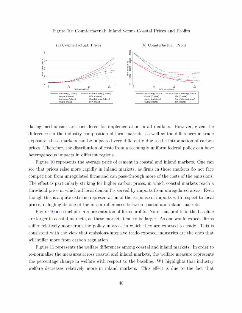
Figure 10: Counterfactual: Inland versus Coastal Prices and Profits

(a) Counterfactual: Prices60

8010

012

014

0C

emen

t pric

e ($

/ton)

0 20 40 60CO2 price ($/ton)

Auctioning (Coastal) Grandfathering (Coastal)Output (Coastal) BTA (Coastal)Auctioning (Inland) Grandfathering (Inland)Output (Inland) BTA (Inland)

(b) Counterfactual: Profit

050

0010

000

1500

020

000

Firm

pro

fits

($ M

)

0 20 40 60CO2 price ($/ton)

Auctioning (Coastal) Grandfathering (Coastal)Output (Coastal) BTA (Coastal)Auctioning (Inland) Grandfathering (Inland)Output (Inland) BTA (Inland)

dating mechanisms are considered for implementation in all markets. However, given the

differences in the industry composition of local markets, as well as the differences in trade

exposure, these markets can be impacted very differently due to the introduction of carbon

prices. Therefore, the distribution of costs from a seemingly uniform federal policy can have

heterogeneous impacts in different regions.

Figure 10 represents the average price of cement in coastal and inland markets. One can

see that prices raise more rapidly in inland markets, as firms in those markets do not face

competition from unregulated firms and can pass-through more of the costs of the emissions.

The effect is particularly striking for higher carbon prices, in which coastal markets reach a

threshold price in which all local demand is served by imports from unregulated areas. Even

though this is a quite extreme representation of the response of imports with respect to local

prices, it highlights one of the major differences between coastal and inland markets.

Figure 10 also includes a representation of firms profits. Note that profits in the baseline

are larger in coastal markets, as these markets tend to be larger. As one would expect, firms

suffer relatively more from the policy in areas in which they are exposed to trade. This is

consistent with the view that emissions-intensive trade-exposed industries are the ones that

will suffer more from carbon regulation.

Figure 11 represents the welfare differences among coastal and inland markets. In order to

re-normalize the measures across coastal and inland markets, the welfare measure represents

the percentage change in welfare with respect to the baseline. W1 highlights that industry

welfare decreases relatively more in inland markets. This effect is due to the fact that

48

demand is inelastic and there are no imports to serve the market. W2 shows that accounting

for emissions reductions in the market has similar effects to both inland and coastal markets,

relatively favoring grandfathering and auctioning with respect to updating mechanisms due

to the full internalization of emissions costs and, thus, lower emissions. For inland markets,

the net benefits of the carbon policy in the industry, accounting for the positive externalities

of emissions reduction, is much more favorable than for coastal markets.

Finally, W3 shows that for sufficiently large abatement costs, coastal market underper-

form in terms of welfare. The intuition is that on those markets, due to the presence of

imports, there is a poor internalization of emissions costs, given that imports attenuate the

degree of pass-through in the market. At high carbon social costs, those emissions are par-

ticularly harmful in terms of welfare. It is also remarkable that for lower prices, both inland

and coastal markets suffer net welfare losses from the regulation and, if anything, coastal

markets tend to suffer less. The intuition is that at lower prices, reductions in emissions are

not valuable and therefore serving the market relatively dominates in terms of welfare. In

coastal markets, the market is better served due to more flexible and cheaper production.

7.3 Robustness checks

7.3.1 Demand and import elasticities

One of the important parameters of the model that affect the computation of welfare mea-

sures is demand elasticity. In order to assess the robustness of our results, we simulate a

subset of markets under different demand elasticities.

The qualitative results are robust to a wide range of demand elasticity estimates, which

are a key determinant of the consumer gross surplus in the model and therefore an important

element in our welfare measures. Appendix C presents a table with W3 welfare differences

for different carbon prices and elasticities. As one would expect, we find that the negative

effects are even more persistent when demand is more inelastic, due to the Buchanan effect,

but still present for more elastic demand curves.

We also consider a wide range of import supply elasticities. Our import supply is exoge-

nous and therefore might underestimate the response of importing firms to increasing cement

prices. By allowing for a more or less responsive supply curve, we capture in a crude way

the possibility of different short-run import responses. Overall, we find that the qualitative

results are unaffected by changing the import supply elasticity.

49

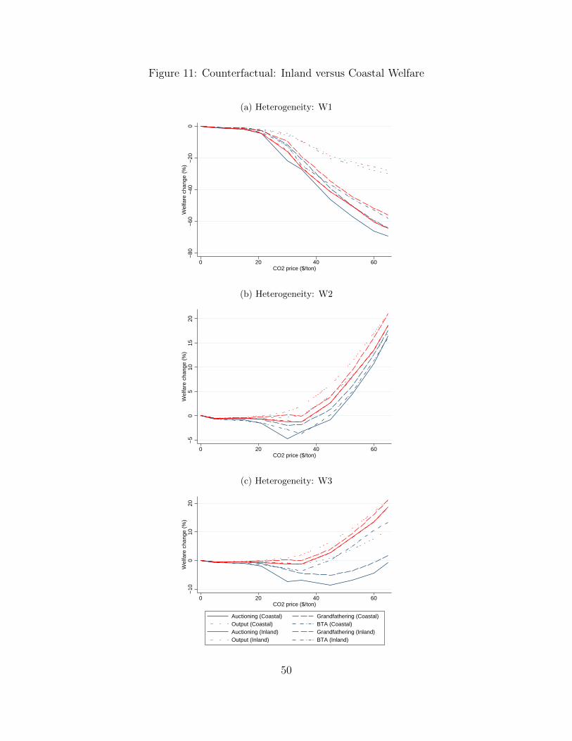
Figure 11: Counterfactual: Inland versus Coastal Welfare

(a) Heterogeneity: W1

−80

−60

−40

−20

0W

elfa

re c

hang

e (%

)

0 20 40 60CO2 price ($/ton)

(b) Heterogeneity: W2

−5

05

1015

20W

elfa

re c

hang

e (%

)

0 20 40 60CO2 price ($/ton)

(c) Heterogeneity: W3

−10

010

20W

elfa

re c

hang

e (%

)

0 20 40 60CO2 price ($/ton)

Auctioning (Coastal) Grandfathering (Coastal)Output (Coastal) BTA (Coastal)Auctioning (Inland) Grandfathering (Inland)Output (Inland) BTA (Inland)

50

7.3.2 Output- vs. Emissions-based updating

As a robustness check, we consider incorporates emissions-based rebating. This works in

precisely the same way as output-based rebating, except that rebates (in the form of recycled

tax revenues or free emissions permits) are allocated based on emissions. The more emissions

intensive a firm, the larger the rebate (per unit of outpu) it recieves. This design has been

proposed in cases where firms owning older, less efficient kilns insist that they should be

entitled to a larger allowance allocation so as to compensate them for their higher compliance

costs.

Outcomes differ only slightly across the output-based and emissions-based updating

regimes. The reason is two-fold: first, new firms enter at a fixed frontier emissions rate,

so as the industry turns over we asymptote towards having identical outcomes under both

policies. Second, among incumbents, the only margin for differences between the two is

differential reorganization of production across units with different emissions intensity. This

margin is relatively small compared to the overall contraction in market quantity; as such,

differences between the two policies are masked by the overall market changes.

7.3.3 Carbon Prices and the Social Costs of Carbon

One important assumption that we make is that the carbon price equals the social cost of

carbon. We examine what would happen if there is a divergence between these two terms.

In particular, we analyze what happens when we move carbon prices while holding the true

SCC at $21/ton.

Figure 12 presents welfare measure W3 under this assumption. The picture is very

different from the previous W3 measure, as now there are no positive welfare effects at high

carbon prices. On the contrary, the picture resembles more the welfare measure W1 at those

high prices, as the benefits from the emissions reductions are relatively minor compared to

the carbon price. It is remarkable that not even at lower carbon prices the policy manages

to induce welfare improving reductions.

The picture is different if we look at SCC = $35, as shown in figure 13. In this case, it

can be welfare improving to induce some abatement in the cement industry, although not

at the full cost of carbon. In the case of auctioning and grandfathering, the policies induce

positive welfare when the cost faced by the firms is below $30, being lowest for the auctioning

scenario. Given the implicit subsidy inherent in the output-based mechanism, the policy is

welfare improving for a wider range of prices in that case.

51

Figure 12: Carbon prices at SCC = $21

−30

000

−20

000

−10

000

0W

elfa

re c

hang

e (m

illio

ns o

f dol

lars

)

0 20 40 60CO2 price ($/ton)

Auctioning (Dynamic) Grandfathering (Dynamic)Output (Dynamic) BTA (Dynamic)

Figure 13: Carbon prices at SCC = $35

−20

000

−15

000

−10

000

−50

000

Wel

fare

cha

nge

(mill

ions

of d

olla

rs)

0 20 40 60CO2 price ($/ton)

Auctioning (Dynamic) Grandfathering (Dynamic)Output (Dynamic) BTA (Dynamic)

52

8 Conclusion

We present a dynamic model to evaluate the welfare impacts of market-based regulation of

carbon dioxide emissions in the US cement industry. We assess the implications of several

alternative policy designs, including those that incorporate both an emissions disincentive

(a tax or an obligation to hold an emissions permit) and a production incentive. Simulation

results reported in this working paper pertain to only a subset of regional markets. The

analysis will ultimately include the entire domestic cement sector.

We find that both the magnitude and the sign of the welfare impacts we estimate depend

significantly on how the policy is implemented and what we assume for the social cost of

carbon. At low to moderate carbon values, our results echo Buchanan (1969). Market-based

emissions regulation that internalizes the full emissions externality leads to small social losses.

These losses are exacerbated by emissions leakage in trade exposed regional markets.

At higher carbon values, our results are more in line with Oates and Strassman (1984) who

argue that the welfare gains from pollution control will be large relative to losses associated

with output contraction and the exercise of market power.

Notably, we find that policy designs that incorporate both an emissions penalty and

a production incentive in the form of a rebate welfare dominate more conventional policy

designs. Intuitively, the production incentive works to mitigate leakage in trade exposed

cement markets and the distortion associated with the exercise of market power.

Of course, these simulation results condition on the structural assumptions that define the

underlying model. The higher the carbon price we consider, the farther out counterfactual

is from the data we observe, and the more sensitive our simulation results will be to our

modeling assumptions.

Policy makers are very interested in understanding how proposed climate change policies

would impact strategic, emissions intensive sectors such as the cement industry. The scale

and scope of these policy interventions are unprecedented, making it difficult to anticipate

how industry will respond and what that response will imply for social welfare. Findings

presented in this paper help illustrate the general forces shaping the interaction of market

structure and proposed carbon regulations and provide important insights into the efficiency

and distributional properties of leading policy design alternatives.

53

References

Benitez-Silva, H., Rust, J., Hitsch, G., Pauletto, G., and Hall, G. (2000). A comparison

of discrete and parametric methods for continuous-state dynamic programming problems.

Computing in Economics and Finance 2000 24, Society for Computational Economics.

Bernheim, B. D. and Whinston, M. D. (1990). Multimarket contact and collusive behavior.

RAND Journal of Economics, 21(1):1–26.

Bohringer, C. and Lange, A. (2005). Economic implications of alternative allocation schemes

for emission allowances. The Scandinavian Journal of Economics, 107(3):563–581.

Borenstein, S., Bushnell, J. B., and Wolak, F. A. (2002). Measuring market inefficien-

cies in california’s restructured wholesale electricity market. American Economic Review,

92(5):1376–1405.

Buchanan, J. M. (1969). External diseconomics, corrective taxes, and market structure. The

American Economic Review, 59(1):174–7.

Bushnell, J. and Chen, Y. (2009). Regulation, allocation, and leakage in cap-and-trade

markets for co2. Technical report, EI@Haas WP-183, Washington, DC.

Bushnell, J., Mansur, E., and Saravia, C. (2008). Vertical arrangements, Market Structure,

and competition: an analysis of restructured US electricity markets. American Economic

Review, 98(1):237–266.

Cropper, M. L. and Oates, W. E. (1992). Environmental economics: A survey. Journal of

Economic Literature, 30(2):675–740.

de Boor, C. (2001). A Practical Guide to Splines. Revised Edition. Springer-Verlag New

York Inc.

Doraszelksi, U. and Satterthwaite, M. (2010). Computable markov-perfect industry dynam-

ics. RAND Journal of Economics, 41(2):215–243.

Doraszelski, U. and Pakes, A. (2007). A framework for applied dynamic analysis in io. In

Armstrong, M. and Porter, R., editors, Handbook of Industrial Organization, volume 3,

chapter 30, pages 1888–1966. Elsevier.

54

Ericson, R. and Pakes, A. (1995). Markov perfect industry dynamics: A framework for

empirical work. Review of Economic Studies, 62(1):53–82.

Foster, L., Haltiwanger, J., and Syverson, C. (2008). Reallocation, firm turnover, and effi-

ciency: Selection on productivity or profitability? American Economic Review, 98(1):394–

425.

Fowlie, M. and Muller, N. (2010). Designing markets for pollution when damages vary across

sources: Evidence from the NOx budget program. Technical report.

Greenstone, M., Kopits, E., and Wolverton, A. (2011). Estimating the social cost of carbon

for use in u.s. federal rulemakings: A summary and interpretation. NBER Working Papers

16913, National Bureau of Economic Research, Inc.

Habermann, C. and Kindermann, F. (2007). Multidimensional spline interpolation: Theory

and applications. Comput. Econ., 30(2):153–169.

Humphreys, K. K. and Mahasenan, N. (2001). Towards a sustainable cement industry:

substudy 8. Technical report.

Jans, I. and Rosenbaum, D. I. (1997). Multimarket contact and pricing: Evidence from the

U.S. cement industry. International Journal of Industrial Organization, 15:391–412.

Joskow, P. L. and Kahn, E. (2002). A quantitative analysis of pricing behavior in california’s

wholesale electricity market during summer 2000. The Energy Journal, 23:1–35.

Judd, K. (1998). Numerical Methods in Economics. MIT Press.

Mahasenan, N., Dahowski, R., and Davidson, C. (2005). Greenhouse Gas Control Tech-

nologies, Volume I, chapter The Role of Carbon Dioxide Capture and Sequestration in

Reducing Emissions from Cement Plants in North America. Elsevier Science.

Maskin, E. and Tirole, J. (1988). A theory of dynamic oligopoly, i: Overview and quantity

competition with large fixed costs. Econometrica, 56:549–69.

Miller, N. H. and Osborne, M. (2010). Competition among Spatially Differentiated Firms:

An Estimator with an Application to Cement. EAG Working Paper 10-2.

Millimet, D. L., Roy, S., and Sengupta, A. (2009). Environmental regulations and economic

activity: Influence on market structure. Annual Review of Resource Economics, 1:99–117.

55

Oates, W. E. and Strassman, D. L. (1984). Effluent fees and market structure. Journal of

Public Economics, 24(1):29–46.

Pakes, A. and McGuire, P. (1994). Computing markov-perfect nash equilibria: numerical

implications of a dynamic differentiated product model. RAND Journal of Economics,

25(4):555–589.

Ponssard, J.-P. and Thomas, C. (2010). Capacity investment under demand uncertainty. an

empirical study of the us cement industry, 1994-2006. Technical report.

Puller, S. (2007). Pricing and firm conduct in California’s deregulated electricity market.

The Review of Economics and Statistics, 89(1):75–87.

Ryan, S. P. (2011). The cost of environmental regulation in a concentrated industry. MIT

Working Paper.

Ryan, S. P. and Tucker, C. E. (2010). Diversification and the dynamics of technology

adoption. Conditionally accepted at Quantitative Marketing and Economics.

Sterner, T. (1990). Energy Efficiency and Capital Embodied Technical Change: The Case

of Mexican Cement Manufacturing. The Energy Journal, 11(2):155–168.

Sterner, T. and Isaksson, L. H. (2006). Refunded emission payments theory, distribution of

costs, and swedish experience of nox abatement. Ecological Economics, 57(1):93–106.

Sterner, T. and Muller, A. (2008). Output and abatement effects of allocation readjustment

in permit trade. Climatic Change, 86(1-2):33–49.

Sweeting, A. (2007). Market power in the england and wales wholesale electricity market

1995–2000. Economic Journal, 117(520):654–85.

Wolfram, C. (1999). Measuring duopoly power in the British electricity spot market. The

American Economic Review, 89(4):805–826.

Worrell, E., Price, L., Martin, N., Hendriks, C., and Meida, L. O. (2001). Carbon Dioxide

Emissions from the Global Cement Industry. Annual Review of Energy and the Environ-

ment, 26(1):303–329.

56

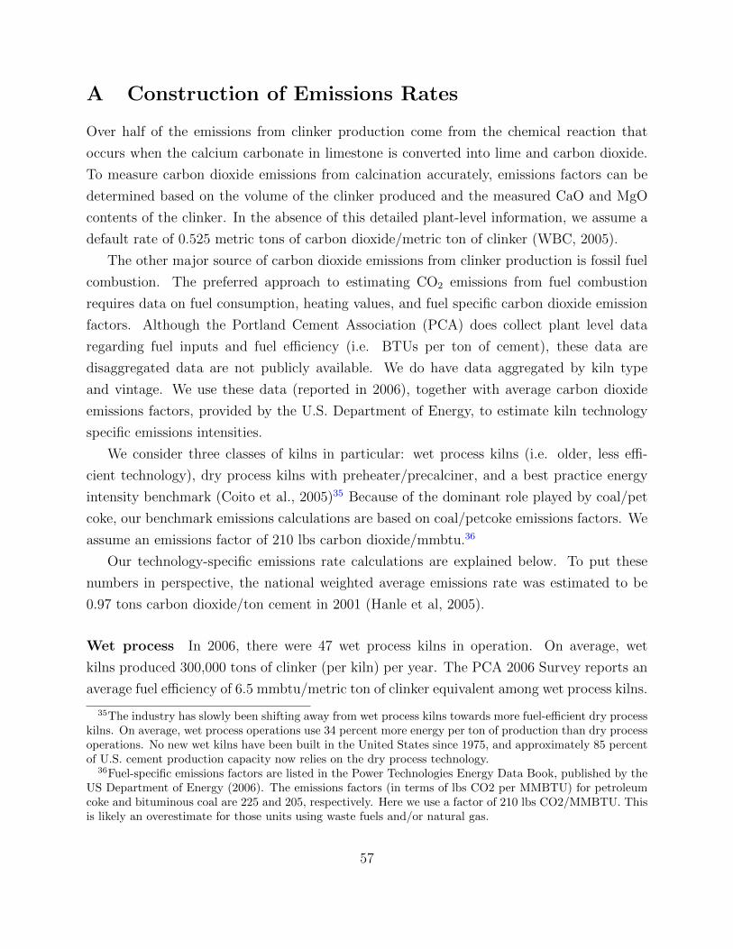
A Construction of Emissions Rates

Over half of the emissions from clinker production come from the chemical reaction that

occurs when the calcium carbonate in limestone is converted into lime and carbon dioxide.

To measure carbon dioxide emissions from calcination accurately, emissions factors can be

determined based on the volume of the clinker produced and the measured CaO and MgO

contents of the clinker. In the absence of this detailed plant-level information, we assume a

default rate of 0.525 metric tons of carbon dioxide/metric ton of clinker (WBC, 2005).

The other major source of carbon dioxide emissions from clinker production is fossil fuel

combustion. The preferred approach to estimating CO2 emissions from fuel combustion

requires data on fuel consumption, heating values, and fuel specific carbon dioxide emission

factors. Although the Portland Cement Association (PCA) does collect plant level data

regarding fuel inputs and fuel efficiency (i.e. BTUs per ton of cement), these data are

disaggregated data are not publicly available. We do have data aggregated by kiln type

and vintage. We use these data (reported in 2006), together with average carbon dioxide

emissions factors, provided by the U.S. Department of Energy, to estimate kiln technology

specific emissions intensities.

We consider three classes of kilns in particular: wet process kilns (i.e. older, less effi-

cient technology), dry process kilns with preheater/precalciner, and a best practice energy

intensity benchmark (Coito et al., 2005)35 Because of the dominant role played by coal/pet

coke, our benchmark emissions calculations are based on coal/petcoke emissions factors. We

assume an emissions factor of 210 lbs carbon dioxide/mmbtu.36

Our technology-specific emissions rate calculations are explained below. To put these

numbers in perspective, the national weighted average emissions rate was estimated to be

0.97 tons carbon dioxide/ton cement in 2001 (Hanle et al, 2005).

Wet process In 2006, there were 47 wet process kilns in operation. On average, wet

kilns produced 300,000 tons of clinker (per kiln) per year. The PCA 2006 Survey reports an

average fuel efficiency of 6.5 mmbtu/metric ton of clinker equivalent among wet process kilns.

35The industry has slowly been shifting away from wet process kilns towards more fuel-efficient dry processkilns. On average, wet process operations use 34 percent more energy per ton of production than dry processoperations. No new wet kilns have been built in the United States since 1975, and approximately 85 percentof U.S. cement production capacity now relies on the dry process technology.

36Fuel-specific emissions factors are listed in the Power Technologies Energy Data Book, published by theUS Department of Energy (2006). The emissions factors (in terms of lbs CO2 per MMBTU) for petroleumcoke and bituminous coal are 225 and 205, respectively. Here we use a factor of 210 lbs CO2/MMBTU. Thisis likely an overestimate for those units using waste fuels and/or natural gas.

57

The relevant conversion is then 0.095 metric tons carbon dioxide/mmbtu * 6.5 mmbtu/metric

ton of clinker equivalent = 0.62 tons carbon dioxide/ton clinker. When added to process

emissions, we obtain our estimate of 1.16 tons carbon dioxide/ton clinker.

Dry process In 2006, there were 54 dry kilns equipped with precalciners with an average

annual output of 1,000,000 tons of clinker per year. The PCA 2006 Survey reports an average

fuel efficiency of 4.1 mmbtu/metric ton of clinker equivalent among dry process kilns with

precalciners. Thus, 0.095 metric tons carbon dioxide/mmbtu * 4.1 mmbtu/metric ton of

clinker equivalent = 0.39 tons carbon dioxide/ton clinker. Adding this to process emissions

results in the estimate for dry-process kilns: 0.93 tons carbon dioxide/ton clinker.

Frontier technology To establish estimates for new entrants, a recent study (Coito et

al, 2005) establishes a best practice standard of 2.89 mmbtu/ metric ton of clinker (not

clinker equivalent). The calculation is then: 0.095 metric tons carbon dioxide/mmbtu * 2.89

mmbtu/metric ton of clinker equivalent= 0.275 tons carbon dioxide/ton clinker. Adding this

to process emissions obtains in 0.81 tons carbon dioxide/ton clinker for new kilns.37

B Abatement response

In the simulation exercise, the state space is modified such that emissions rates vary systemat-

ically across plants of different vintages and technology types. Incumbent firms are classified

as either wet-process, dry-process, or dry-process with precalciner/preheaters. New kilns are

assumed to be state-of-the-art. This modification allows us to crudely capture changes in

embodied emissions intensity as the industry evolves.

There are four main strategies for reducing the carbon intensity of domestic cement

industry. First, it is anticipated that capital stock turnover will be a major driver of emissions

intensity reductions (Worrell, 1999). Replacing old wet-process kilns with state-of-the-art

dry kilns could deliver significant reductions in combustion-related emissions.

Second, the carbon intensity of clinker production can also be reduced via fuel switching.

Currently, coal and petroleum coke are overwhelmingly the dominant fuel used in pyropro-

cessing and electricity is used to grind raw materials into kiln feed. Most domestic kilns are

37This is very similar to the CO2 emissions rate assumed in analyses carried out by California’s AirResources Board in 2008 under a best practice scenario that does not involve fuel switching. If fuel switchingis assumed, best practice emissions rates drop as low as 0.69 MT CO2/ MT cement. See NRDC CementGHG Reduction Final Calculations.

58

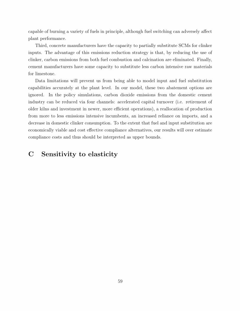
capable of burning a variety of fuels in principle, although fuel switching can adversely affect

plant performance.

Third, concrete manufacturers have the capacity to partially substitute SCMs for clinker

inputs. The advantage of this emissions reduction strategy is that, by reducing the use of

clinker, carbon emissions from both fuel combustion and calcination are eliminated. Finally,

cement manufacturers have some capacity to substitute less carbon intensive raw materials

for limestone.

Data limitations will prevent us from being able to model input and fuel substitution

capabilities accurately at the plant level. In our model, these two abatement options are

ignored. In the policy simulations, carbon dioxide emissions from the domestic cement

industry can be reduced via four channels: accelerated capital turnover (i.e. retirement of

older kilns and investment in newer, more efficient operations), a reallocation of production

from more to less emissions intensive incumbents, an increased reliance on imports, and a

decrease in domestic clinker consumption. To the extent that fuel and input substitution are

economically viable and cost effective compliance alternatives, our results will over estimate

compliance costs and thus should be interpreted as upper bounds.

C Sensitivity to elasticity

59

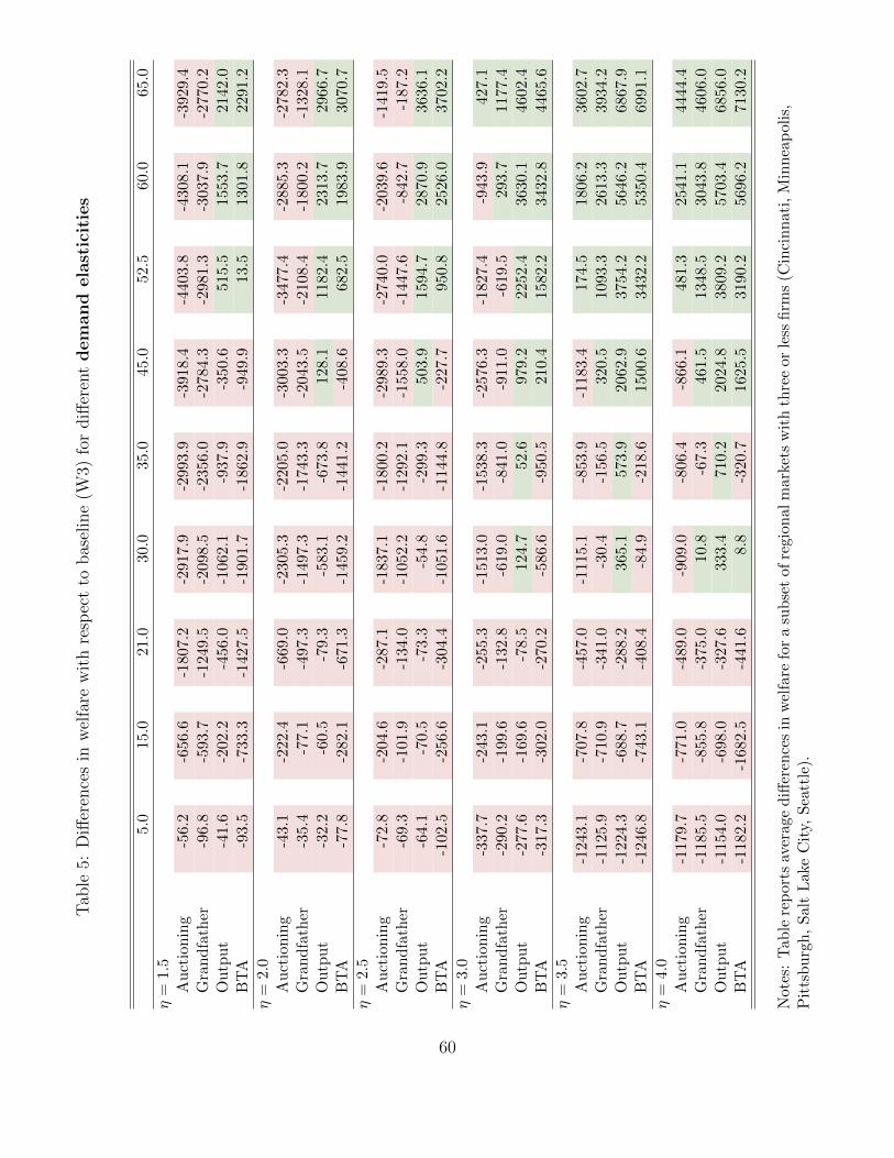
Tab

le5:

Diff

eren

ces

inw

elfa

rew

ith

resp

ect

tobas

elin

e(W

3)fo

rdiff

eren

tdem

and

ela

stic

itie

s

5.0

15.

021

.030

.035

.045

.052

.560

.065

.0

η=

1.5

Au

ctio

nin

g-5

6.2

-656.

6-1

807.

2-2

917.

9-2

993.

9-3

918.

4-4

403.

8-4

308.

1-3

929.

4G

ran

dfa

ther

-96.

8-5

93.

7-1

249.

5-2

098.

5-2

356.

0-2

784.

3-2

981.

3-3

037.

9-2

770.

2O

utp

ut

-41.

6-2

02.

2-4

56.0

-106

2.1

-937

.9-3

50.6

515.

515

53.7

2142

.0B

TA

-93.

5-7

33.

3-1

427.

5-1

901.

7-1

862.

9-9

49.9

13.5

1301

.822

91.2

η=

2.0

Au

ctio

nin

g-4

3.1

-222.

4-6

69.0

-230

5.3

-220

5.0

-300

3.3

-347

7.4

-288

5.3

-278

2.3

Gra

nd

fath

er-3

5.4

-77.

1-4

97.3

-149

7.3

-174

3.3

-204

3.5

-210

8.4

-180

0.2

-132

8.1

Ou

tpu

t-3

2.2

-60.

5-7

9.3

-583

.1-6

73.8

128.

111

82.4

2313

.729

66.7

BT

A-7

7.8

-282.

1-6

71.3

-145

9.2

-144

1.2

-408

.668

2.5

1983

.930

70.7

η=

2.5

Au

ctio

nin

g-7

2.8

-204.

6-2

87.1

-183

7.1

-180

0.2

-298

9.3

-274

0.0

-203

9.6

-141

9.5

Gra

nd

fath

er-6

9.3

-101.

9-1

34.0

-105

2.2

-129

2.1

-155

8.0

-144

7.6

-842

.7-1

87.2

Ou

tpu

t-6

4.1

-70.

5-7

3.3

-54.

8-2

99.3

503.

915

94.7

2870

.936

36.1

BT

A-1

02.5

-256.

6-3

04.4

-105

1.6

-114

4.8

-227

.795

0.8

2526

.037

02.2

η=

3.0

Au

ctio

nin

g-3

37.7

-243.

1-2

55.3

-151

3.0

-153

8.3

-257

6.3

-182

7.4

-943

.942

7.1

Gra

nd

fath

er-2

90.2

-199.

6-1

32.8

-619

.0-8

41.0

-911

.0-6

19.5

293.

711

77.4

Ou

tpu

t-2

77.6

-169.

6-7

8.5

124.

752

.697

9.2

2252

.436

30.1

4602

.4B

TA

-317.3

-302.

0-2

70.2

-586

.6-9

50.5

210.

415

82.2

3432

.844

65.6

η=

3.5

Au

ctio

nin

g-1

243

.1-7

07.

8-4

57.0

-111

5.1

-853

.9-1

183.

417

4.5

1806

.236

02.7

Gra

nd

fath

er-1

125

.9-7

10.

9-3

41.0

-30.

4-1

56.5

320.

510

93.3

2613

.339

34.2

Ou

tpu

t-1

224

.3-6

88.

7-2

88.2

365.

157

3.9

2062

.937

54.2

5646

.268

67.9

BT

A-1

246

.8-7

43.

1-4

08.4

-84.

9-2

18.6

1500

.634

32.2

5350

.469

91.1

η=

4.0

Au

ctio

nin

g-1

179

.7-7

71.

0-4

89.0

-909

.0-8

06.4

-866

.148

1.3

2541

.144

44.4

Gra

nd

fath

er-1

185

.5-8

55.

8-3

75.0

10.8

-67.

346

1.5

1348

.530

43.8

4606

.0O

utp

ut

-1154

.0-6

98.

0-3

27.6

333.

471

0.2

2024

.838

09.2

5703

.468

56.0

BT

A-1

182

.2-1

682.

5-4

41.6

8.8

-320

.716

25.5

3190

.256

96.2

7130

.2

Note

s:T

ab

lere

por

tsav

erag

ed

iffer

ence

sin

wel

fare

for

asu

bse

tof

regi

onal

mar

kets

wit

hth

ree

orle

ssfi

rms

(Cin

cin

nat

i,M

inn

eap

olis

,P

itts

bu

rgh

,S

alt

Lake

Cit

y,S

eatt

le).

60

Tab

le6:

Diff

eren

ces

inw

elfa

rew

ith

resp

ect

tobas

elin

e(W

3)fo

rdiff

eren

tim

port

ela

stic

itie

s

5.0

15.0

21.0

30.0

35.0

45.0

52.5

60.0

65.0

η=

1.5

Au

ctio

nin

g-1

76.

3-1

17.8

-158

.9-1

345.

8-1

215.

9-2

221.

7-3

814.

0-8

84.4

-51.

7G

ran

dfa

ther

-176.

3-1

03.4

-59.

7-7

60.3

-838

.7-1

080.

2-8

50.2

-84.

663

0.7

Ou

tpu

t-1

72.

4-1

00.7

-61.

6-2

2.7

-311

.244

6.4

1260

.322

17.7

2705

.8B

TA

-198.

9-1

58.5

-191

.9-8

18.2

-809

.5-1

9.0

887.

016

82.9

2594

.0

η=

2.0

Au

ctio

nin

g-1

80.

8-1

19.5

-158

.9-1

433.

3-1

283.

2-2

459.

7-2

048.

4-1

573.

1-6

68.3

Gra

nd

fath

er-1

80.

0-1

08.0

-61.

8-4

89.6

-866

.5-1

219.

4-1

208.

9-6

64.1

-87.

9O

utp

ut

-176.

1-1

06.0

-65.

5-1

0.6

-274

.534

2.8

1133

.920

55.9

2530

.1B

TA

-203.

5-1

71.6

-215

.5-7

01.8

-785

.534

.795

1.3

2065

.127

06.9

η=

2.5

Au

ctio

nin

g-2

36.

5-1

27.4

-164

.8-1

463.

4-1

344.

6-2

667.

5-2

398.

6-2

096.

4-1

205.

3G

ran

dfa

ther

-195.

5-1

17.8

-68.

7-6

22.9

-886

.0-1

340.

6-1

515.

4-1

198.

0-7

55.6

Ou

tpu

t-1

88.

3-1

15.8

-72.

0-1

9.0

-212

.225

1.2

996.

018

08.2

2389

.3B

TA

-216.

0-1

86.0

-185

.0-5

37.0

-756

.911

9.2

1010

.922

80.3

2833

.2

η=

3.0

Au

ctio

nin

g-3

37.

8-1

68.2

-195

.3-1

080.

5-1

393.

3-2

824.

7-2

689.

0-2

513.

8-1

651.

6G

ran

dfa

ther

-253.

5-1

60.5

-343

.1-7

10.8

-907

.1-1

427.

6-1

786.

8-1

671.

8-1

332.

4O

utp

ut

-306.

3-1

57.9

-101

.6-3

7.0

-216

.619

1.3

940.

217

42.7

2338

.2B

TA

-315.

5-2

46.4

-194

.0-5

09.3

-723

.618

6.1

1088

.424

00.8

3199

.9

η=

3.5

Au

ctio

nin

g-3

85.

2-2

75.2

-728

.2-1

250.

6-1

315.

2-2

753.

2-2

689.

4-2

579.

5-1

690.

9G

ran

dfa

ther

-343.

2-1

82.2

-78.

6-3

60.8

-764

.4-1

296.

0-1

775.

0-1

820.

0-1

487.

6O

utp

ut

-367.

8-1

91.6

-83.

461

.3-1

26.2

323.

011

41.3

1952

.826

39.9

BT

A-3

83.

7-2

19.5

-146

.7-3

19.6

-516

.045

4.8

1434

.728

07.6

3667

.7

η=

4.0

Au

ctio

nin

g-4

94.

3-2

94.5

-249

.3-1

430.

2-1

379.

3-2

882.

5-2

931.

5-2

904.

0-2

000.

6G

ran

dfa

ther

-494.

3-2

87.7

-155

.0-3

78.5

-809

.8-1

365.

8-1

999.

0-2

245.

8-1

856.

0O

utp

ut

-488.

7-2

86.3

-156

.516

.3-8

3.5

259.

810

57.6

1966

.025

95.2

BT

A-5

20.

0-2

97.3

-195

.8-3

31.2

-506

.450

2.3

1501

.328

97.6

3925

.5

Note

s:T

ab

lere

por

tsav

erag

ed

iffer

ence

sin

wel

fare

for

asu

bse

tof

regi

onal

mar

kets

wit

hth

ree

orle

ssfi

rms

(Cin

cin

nat

i,M

inn

eap

olis

,S

eatt

le).

61