ABSTRACT

CHANCEY, MARK ALAN. Short Range Underwater Optical Communication Links. (Under the direction of Dr. John F. Muth)

The future tactical ocean environment will be increasingly complicated. In addition

to traditional communication links there will be a proliferation of unmanned vehicles in

space, in the air, on the surface, and underwater. To effectively utilize these systems

improvements in underwater communication systems are needed. Since radio waves do not

propagate in sea water, and acoustic communication systems are relatively low bandwidth

the possibility of high speed underwater optical communication systems are considered.

In traditional communication systems, constructing a link budget is often relatively

straight forward. In the case of underwater optical systems the variations in the optical

properties of ocean water lead to interesting problems when considering the feasibility and

reliability of underwater optical links. The main focus of this thesis is to understand how to

construct an underwater link budget which includes the effects of scattering and absorption

of realistic ocean water.

The secondary focus of the thesis was to construct LED based optical communication

systems. This required understanding the behavior of Gallium Nitride LEDs operated under

intense electrical pulsing conditions. An optical FM wireless system was constructed for

transmitting speech. An LED based Ethernet compatible digital communications system that

was capable of operating at 10 Mbps was also constructed and packaged for underwater

operation.

SHORT RANGE UNDERWATER OPTICAL

COMMUNICATION LINKS

By

MARK ALAN CHANCEY

A thesis submitted to the Graduate Faculty of North Carolina State University

in partial fulfillment of the requirements for the Degree of

Master of Science

ELECTRICAL ENGINEERING

Raleigh, NC

2005

APPROVED BY:

___________________________ __________________________ Professor John F. Muth Professor Gianluca Lazzi

Chair of Advisory Committee

________________________________ Professor Leda Lunardi

ii

DEDICATIONS

This is for:

My father J. Lamar Chancey, who always pushed me to my limits.

My mother Barbara F. Swain,

who always supported my decisions.

AND

My wife Erin G. Chancey, who loved and supported

me throughout my research

iii

BIOGRAPHY

Mark Alan Chancey was born on April 10, 1980 in a small town of Greensboro North

Carolina. As a child he grew up with a father who was an electrical engineer and inspired

him to push his limits in everything he did.

In June of 1998, Mark graduated from Western Alamance High School third in his

class and was accepted into NC State University for fall of 1998 classes. He started his

college career as a Chemical Engineer, since he was relatively experienced in chemistry.

After his first year Mark decided to switch disciplines, from chemical engineering to

electrical engineering. In the summer of 2000, Mark began dating a childhood friend Erin

Grey Williams. They dated for the rest of his undergraduate degree, even when he moved to

Wilmington, NC to work for Corning Inc for two CO-OP rotations. Mark drove to

Burlington, NC every other weekend to be with her. At Corning the engineers sparked his

interest in optics. Ever day he would learn something new, something that made him more

eager to learn about optics and optical communications. When the stock market took a nose

dive, Corning Inc told Mark that, despite his excellent work they could not bring him back

for a third rotation due to budget cutbacks to complete his CO-OP requirements. To finish

his requirements, he found a local company in Cary, NC called Buehler Motor Inc. There he

studied Electromagnetic Interference (EMI) through conducted and radiated emissions of

automotive motors and actuators.

With his interest for optics and his work experience with Corning, Mark ran across

the path of Dr. J. Muth, who was the optical communications professor at NC State

University.

In May of 2003 Mark graduated, Magna Cum Laude, from NC State University with

his Bachelor’s of Science in Electrical Engineering. After graduation Mark was approached

with the idea of an underwater optical link for his thesis. So in began his research under the

advisement of Dr. J. Muth of the Electrical and Computer Engineering department of NC

State University.

On June 4, 2004, Erin Grey Williams became Mark’s beautiful wife!

iv

ACKNOWLEDGEMENTS

First of all, I would like to thank Jesus Christ and GOD the father for all the blessings

they have given me. Without them, none of this could have been possible. Christ was the

light during my darkest hour and the shoulder that I could rest my weary head on. Even

though I don’t deserve His love, He gives it to me unconditionally and I thank Him, the great

I AM.

I would also like to thank my father. Even though he was tough on me as I was

growing up, he molded me into a mature and independent adult. I would also like to thank

my mother. She always supported me in everything I did or tried. Her caring words and

kind nature taught me how to have fun with life but in a responsible manner.

I can’t forget about my step-parents either. Both my step-parents treated me as if I

was their own son. Through the good time and bad, they both taught me things about life

that I still hold true to myself today.

Of course I can’t for forget my wife, I would like to thank her with all my heart. We

first started out just friends back when we were teenagers. Then, the summer of my

sophomore year in college we started dating. She stayed with me in a long distance

relationship for almost 4 years before she became my wife. With every word she brings

comfort, serenity, and loving support. Even when I’m up late at night studying for a test,

writing my thesis, and searching for jobs, she’s right there by my side. Without her, I

sincerely doubt that I could have made it through school. She is my friend, my soul mate,

my love, basically Every Reason I Needed to fall in Love.

v

TABLE OF CONTENTS Page

LIST OF TABLES.................................................................................................................. vii LIST OF FIGURES ............................................................................................................... viii LIST OF ABBREVIATIONS................................................................................................... x LIST OF SYMBOLS ............................................................................................................... xi Chapter 1 Introduction........................................................................................................... 1

1.1 References................................................................................................................. 3 Chapter 2 Review of Literature ............................................................................................. 4

2.1 Free Space Optics Concepts...................................................................................... 4 2.2 Appling FSO Concepts to Seawater ......................................................................... 6

Water Types ...................................................................................................................... 6 Attenuation Underwater.................................................................................................... 8

2.3 References............................................................................................................... 22 Chapter 3 Link Budget ........................................................................................................ 24

3.1 Computing Free Space Link Budgets ..................................................................... 27 Optical Link Budget Equation ........................................................................................ 27 Geometric Effects in Link Budget .................................................................................. 28 Environmental Consideration in Link Budgets............................................................... 29 FSO Power Link Budget Equation ................................................................................. 30

3.2 RF Link Budget....................................................................................................... 32 Geometric Effects in Link Budget .................................................................................. 32

3.3 Acoustical Link Budget .......................................................................................... 32 Geometric Effects in Link Budget .................................................................................. 32 Environmental Consideration in Link Budgets............................................................... 33

3.4 Underwater Optical Link Budget............................................................................ 34 Geometric Effects in Link Budget .................................................................................. 34 Building an Underwater Link Model.............................................................................. 34

3.5 Link Budget Results................................................................................................ 41 3.6 References............................................................................................................... 44

Chapter 4 Figure of Merits for Underwater Platform.......................................................... 46 4.1 System Level Figure of Merit ................................................................................. 48 4.2 FOM Transmitter .................................................................................................... 49 4.3 FOM Environment .................................................................................................. 51 4.4 FOM Receiver......................................................................................................... 52 4.5 References............................................................................................................... 52

Chapter 5 Experimental Data and Circuitry ........................................................................ 53 5.1 High Powered LEDS............................................................................................... 53 5.2 High Powered Pulser Circuit using ZTX415 Avalanche Transistors ..................... 57 5.3 FM Optical Wireless System .................................................................................. 63

Transmitter...................................................................................................................... 65 Receiver .......................................................................................................................... 67

5.4 RONJA, 10Mbps Optical Data Link....................................................................... 70

vi

Design ............................................................................................................................. 70 5.5 References............................................................................................................... 80

Conclusion/Summary.............................................................................................................. 81 Appendix A............................................................................................................................. 85

MathCAD Code .................................................................................................................. 85 Appendix B ............................................................................................................................. 95

Circuit Diagrams................................................................................................................. 95 Appendix C ............................................................................................................................. 99

Parts List ............................................................................................................................. 99

vii

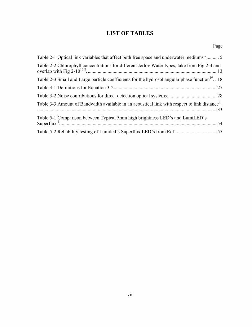
LIST OF TABLES

Page

Table 2-1 Optical link variables that affect both free space and underwater mediums,,, .......... 5

Table 2-2 Chlorophyll concentrations for different Jerlov Water types, take from Fig 2-4 and overlap with Fig 2-1016,8. ........................................................................................................ 13

Table 2-3 Small and Large particle coefficients for the hydrosol angular phase function19. . 18

Table 3-1 Definitions for Equation 3-2................................................................................... 27

Table 3-2 Noise contributions for direct detection optical systems........................................ 28

Table 3-3 Amount of Bandwidth available in an acoustical link with respect to link distance8.................................................................................................................................................. 33

Table 5-1 Comparison between Typical 5mm high brightness LED’s and LumiLED’s Superflux,2............................................................................................................................... 54

Table 5-2 Reliability testing of Lumiled’s Superflux LED’s from Ref ................................. 55

viii

LIST OF FIGURES Page

Figure 2-1 FSO links when no direct link fiber optic network is possible .............................. 4

Figure 2-2 Diagram of the different oceanic zones. ................................................................. 6

Figure 2-3 The spectral transmittance over the upper 10m of water. ....................................... 7

Figure 2-4 World map locating Jerlov water Types I-III......................................................... 7

Figure 2-5 Absorption coefficient as a function of wavelength (nm) for pure seawater. ......... 9

Figure 2-6 Curve fitting of the absorption coefficient as function of chlorophyll.................. 10

Figure 2-7 Chlorophyll depth profile. ..................................................................................... 11

Figure 2-8 Chlorophyll depth profile for different water types. ............................................. 12

Figure 2-9 Satellite remote sensor reading of the chlorophyll-a concentration ..................... 13

Figure 2-10 Absorption coefficient of gelbstoff. .................................................................... 14

Figure 2-11 Scattering coefficient of pure seawater as a function of wavelength (nm). ........ 15

Figure 2-12 The angular distribution of the scattering phase function for pure water. .......... 16

Figure 2-13 Pure seawater absorption coefficient overlapped with scatter coefficient.. ........ 17

Figure 2-14 Overlap plot of the pure seawater phase function............................................... 19

Figure 2-15 Influence of detector angle with respect to the beam axis. ................................. 20

Figure 3-1 Different Communication Systems Expressed as Bitrate Lenth Product.............. 24

Figure 3-2 The limits of the underwater system performance . .............................................. 26

Figure 3-3 Functional bock diagram of the total attenuation in seawater............................... 35

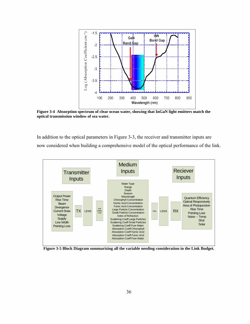
Figure 3-4 Absorption spectrum of clear ocean water............................................................ 36

Figure 3-5 Block Diagram summarizing link budget considerations. .................................... 36

Figure 3-6 The total spectral attenuation coefficient, for several Jerlov water types. ............ 41

Figure 3-7 1 W LED, Type II water with particulate, CDOM, chlorophyll, and scattering... 42

Figure 3-8 10 W laser,Type I water with particulate, CDOM, chlorophyll, and scattering. .. 42

Figure 3-9 1 W laser, Type Ib water with particulate, CDOM, chlorophyll, and scattering. . 43

Figure 4-1 Comparison between Acoustical and Optical Communication underwater. ........ 48

Figure 5-1 Output wavelength from Superflux LED’s: Blue, Green, and Cyan. ................... 54

Figure 5-2 Conventional packaged LED and LumiLED’s package Superflux LED.............. 55

Figure 5-3 Comparison between die of convention LED and a LumiLED . .......................... 56

Figure 5-4 Luxon Star/O package and Luxeon Star/O die image........................................... 56

ix

Figure 5-5 Circuit diagram of 4ns light pulse generator and circuit board ............................ 57

Figure 5-6 I-V characteristics of a ztx415 avalanche transistor. ............................................ 58

Figure 5-7 Oscilloscope reading of a 4ns pulse produced by the above circuit ..................... 59

Figure 5-8 Spectral shift in a Superflux LED using 4ns pulser circuit................................... 60

Figure 5-9 Smooth curve from the Superflux LED with a constant DC source. .................... 60

Figure 5-10 Fabrey-Perot fringes appear a result of the Superflux LED being pulsed. ......... 61

Figure 5-11 First generation FM wireless circuit ................................................................... 63

Figure 5-12 Circuit Diagram of FM 2-way voice LED link................................................... 64

Figure 5-13 Circuit block diagram of FM optical wireless system ........................................ 65

Figure 5-14 Transmitted pulse is 4.25V peak at 111kHz. Graph @ 2V/Div.......................... 67

Figure 5-15 “Locked” 116kHz signal from internal VCO. Graph @ 5V/Div........................ 68

Figure 5-16 “Locked” condition for Phase Locked Loop...................................................... 68

Figure 5-17 Functional block diagram of the Twisted Pair Interface. .................................... 71

Figure 5-18 Functional block diagram of the transmitter board ............................................. 73

Figure 5-19 Functional block diagram of the receiver board ................................................. 74

Figure 5-20 Reciver optical lens system................................................................................. 75

Figure 5-21 Transmitter optical lens system........................................................................... 76

Figure 5-22 Cyan LED through the tank,Green LED transmission through the water tank. . 76

Figure 5-23 Water proof coaxial cable connector and water proofed Lens sealing ............... 77

Figure 5-24 Ronja underwater receiver and transmitter underwater casing. .......................... 78

Figure 5-25 A 10MHz signal after passing through the water tank........................................ 79

x

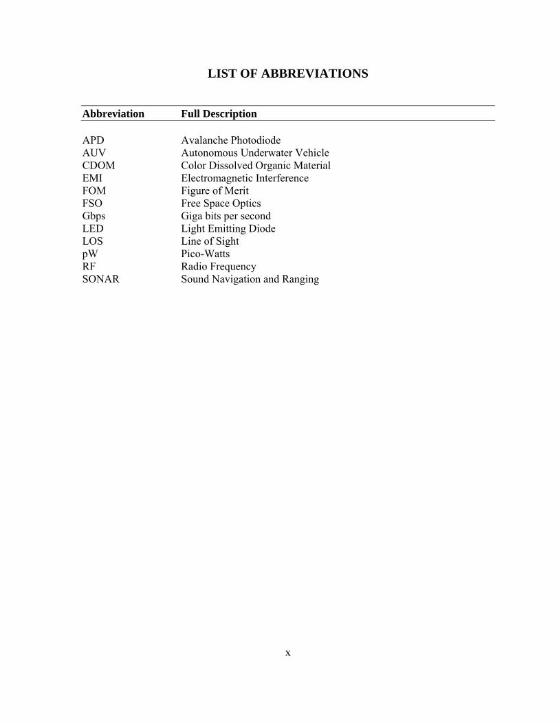
LIST OF ABBREVIATIONS

Abbreviation Full Description APD Avalanche Photodiode AUV Autonomous Underwater Vehicle CDOM Color Dissolved Organic Material EMI Electromagnetic Interference FOM Figure of Merit FSO Free Space Optics Gbps Giga bits per second LED Light Emitting Diode LOS Line of Sight pW Pico-Watts RF Radio Frequency SONAR Sound Navigation and Ranging

xi

LIST OF SYMBOLS Symbol Unit Description

( )λα m-1 Total spectral attenuation coefficient ( )λa m-1 Total spectral absorption coefficient

( )λwa m-1 Absorption coefficient for pure seawater ( )λcla m-1 Absorption coefficient for chlorophyll

( )λoca m-1 Specific absorption coefficient of chlorophyll

( )λfa m-1 Absorption coefficient for fulvic acid

( )λofa m-1 Specific absorption coefficient of fulvic acid

( )λha m-1 Absorption coefficient for humic acid ( )λo

ha m-1 Specific absorption coefficient of humic acid

cC mg/m3 Total concentration of chlorophyll ocC mg/m3 ( )λcla with respect to chlorophyll concentration

fC g/m3 Concentration of fulvic acid

hC g/m3 Concentration of humic acid ( )λb m-1 Total spectral scattering coefficient ( )λob m-1 Scattering coefficient of pure seawater ( )λo

sb m-1 Scattering coefficient of small particles ( )λo

lb m-1 Scattering coefficient of large particles

sC g/m3 Concentration of small particles

lC g/m3 Concentration of large particles ( )φβ w unit less Molecular scattering phase function ( )φλβ ,Hy unit less Total hydrosol phase function ( )φλβ ,H unit less Seawater angular scattering coefficient

( )φρ r unit less Rayleigh phase function ( )φρ s unit less Small particle phase function ( )φρ l unit less Large particle phase function

)(zC mg/m3 Chlorophyll concentration as function of depth

oB mg/m3 Background chlorophyll concentration S mg/m3/m Vertical chlorophyll concentration gradient z m Depth h mg/m2 Total chlorophyll above the background σ unit less Standard deviation of Gaussian distribution

xii

Symbol Unit Description

maxz m Depth of chlorophyll maximum

rP W Optical power received

oP W Initial optical power from transmitter

rD m Diameter of receiving aperture

tD m Diameter of transmitting aperture Div radians Divergence of the optical beam Lm m Distance of optical link

systemFOM Figure of Merit for a system

TxFOM (bps/J)*m*Sr Figure of Merit for transmitter from system

tEnvironmenFOM dB/m Figure of Merit for environmental effects

RxFOM (bps/J)*Sr Figure of Merit for receiver from system

Chapter 1 Introduction

The future tactical ocean environment will be increasingly complicated. In addition

to traditional communication links there will be a proliferation of unmanned vehicles in

space, in the air, on the surface, and underwater. Above the air/water interface wireless radio

frequency communications will continue to provide the majority of communication channels.

Underwater, where radio waves do not propagate, acoustic methods will continue to be used.

However, while there have been substantial advances in acoustic underwater

communications, acoustics will be hard pressed to provide sufficient bandwidth to multiple

platforms at the same time. Acoustic methods will also continue to have difficulty

penetrating the water/air interface. This suggests that high bandwidth, short range

underwater optical communications have high potential to augment acoustic communication

methods.

The variations in the optical properties of ocean water lead to interesting problems when

considering the feasibility and reliability of underwater optical links. Radio waves do not

propagate underwater, however with the proliferation of unmanned autonomous vehicles the

need to communicate large amounts of data is quickly increasing. Making physical

connections underwater to transfer data is often impractical operationally or technically hard

to do. Traditionally most underwater communication systems have been acoustic and

relatively low bandwidth. However, the development of high brightness blue/green LED

sources, and laser diodes suggest that high speed optical links can be viable for short range

applications. Underwater systems also have severe power, and size constraints compared to

land or air based systems.

Underwater vehicles also encounter a wide range of optical environments. In shallow

water the effects of absorption by organic matter and scattering by inorganic particulates can

be severe compared to deep ocean water. Where the system operates in the water column

can also have strong influence. Near the sea floor, ocean currents and silt can play a factor,

while in the middle of the water column the medium may be considered more homogeneous,

but with its optical properties varying as a function of depth. Near the surface, sunlight can

2

provide a strong background signal that needs to be filtered, and the amount of wave action

can have significant effects.

In this thesis the use of free space optical links will be investigated for underwater

applications. With the use of MathCAD, optical link budgets for three different scenarios are

considered:

• A blue/green LED based, bottom moored buoy system operating in relatively shallow

water.

• A blue/green laser based system operating in deep clear ocean water with unlimited

power and size constraints.

• A power and size constrained, diode laser system suitable for small unmanned

underwater vehicle operation.

Inputs into the link budget include: light source type, wavelength, optical power, beam

divergence, ocean water optical parameters based on depth, geographic location and time of

day, and photodetector type. As a point of comparison, the relative merits of these systems

are compared to a conventional acoustic communications links.

A secondary focus of the thesis was to construct light emitting diode based links. The

choice of using LEDs instead of Lasers was largely economic, however in the underwater

environment can be very challenging optically and many of the advantages that lasers have in

terms of beam quality can be rapidly degraded by scattering and turbulence.

A pulsar circuit capable of 4 nanosecond pulses, and 2 Amps per pulse based on the

works of references1,2, and 3 was constructed to study the behavior of LEDs under intense

current injection conditions. The pulser circuit and a simpler pulsed LED circuit were used to

construct a FM optical wireless capable of transmitting voice. The circuit was similar in

concept to the work of Ref 4 and5, but significant modifications were made to the circuit

design.

An Ethernet compatible digital optical communication system was build based on the

open source hardware project “RONJA”, but was modified and packaged for underwater

operation. This system was capable of 10 Mbps operation.

3

1.1 References 1 T. Araki, Y. Fujisawa, M. Hashimoto, “An ultraviolet nanosecond light pulse generator using a light emitting diode for test of photodetectors”, American Institute of Physics, Rev. Sci. Insrum. 68 (3), March 1997 2 R.J. Baker, “High Voltage pulse generation using current mode second breakdown in a bipolar junction transistor”, American Institute of Physics, Rev. Sci. Insrum. 62 (4), April 1991 3 R.V. Vasil’ev, B.K. Lubsandorzhiev, P.G. Pokhil, “A Nanosecond Light Source for Scintillation and Cerenkov-Detector Calibration”, Instrumetns and Experimental Techniques, Vol. 43, No. 4, pg 570-572, 2000 4 G. Pang, T. Kwan, H. Liu, Chi-Ho Chan, “Optical Wireless based on High Brightness Visible LEDs”, IEEE, pg 1693-1698, 1999, 0-7803-5589-X 5 Z. Ghassemlooy, School of Engineering, Northumbria University, Newcastle upon Tyne, UK, A.R. Hayes, Quantum Beam Ltd. UK, “Indoor Optical Wireless Communication Systems- Part I: Review”, pg 11-33 2003

4

Chapter 2 Review of Literature

2.1 Free Space Optics Concepts

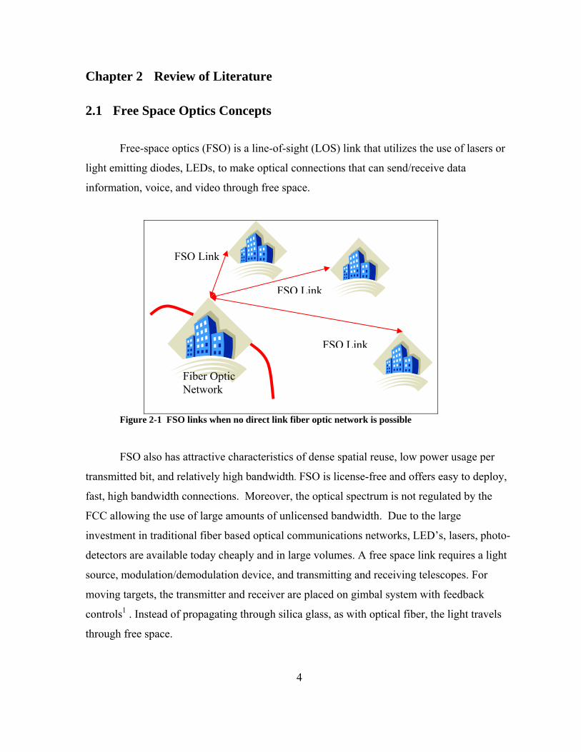
Free-space optics (FSO) is a line-of-sight (LOS) link that utilizes the use of lasers or

light emitting diodes, LEDs, to make optical connections that can send/receive data

information, voice, and video through free space.

Figure 2-1 FSO links when no direct link fiber optic network is possible

FSO also has attractive characteristics of dense spatial reuse, low power usage per

transmitted bit, and relatively high bandwidth. FSO is license-free and offers easy to deploy,

fast, high bandwidth connections. Moreover, the optical spectrum is not regulated by the

FCC allowing the use of large amounts of unlicensed bandwidth. Due to the large

investment in traditional fiber based optical communications networks, LED’s, lasers, photo-

detectors are available today cheaply and in large volumes. A free space link requires a light

source, modulation/demodulation device, and transmitting and receiving telescopes. For

moving targets, the transmitter and receiver are placed on gimbal system with feedback

controls1 . Instead of propagating through silica glass, as with optical fiber, the light travels

through free space.

Fiber Optic Network

FSO Link

FSO Link

FSO Link

5

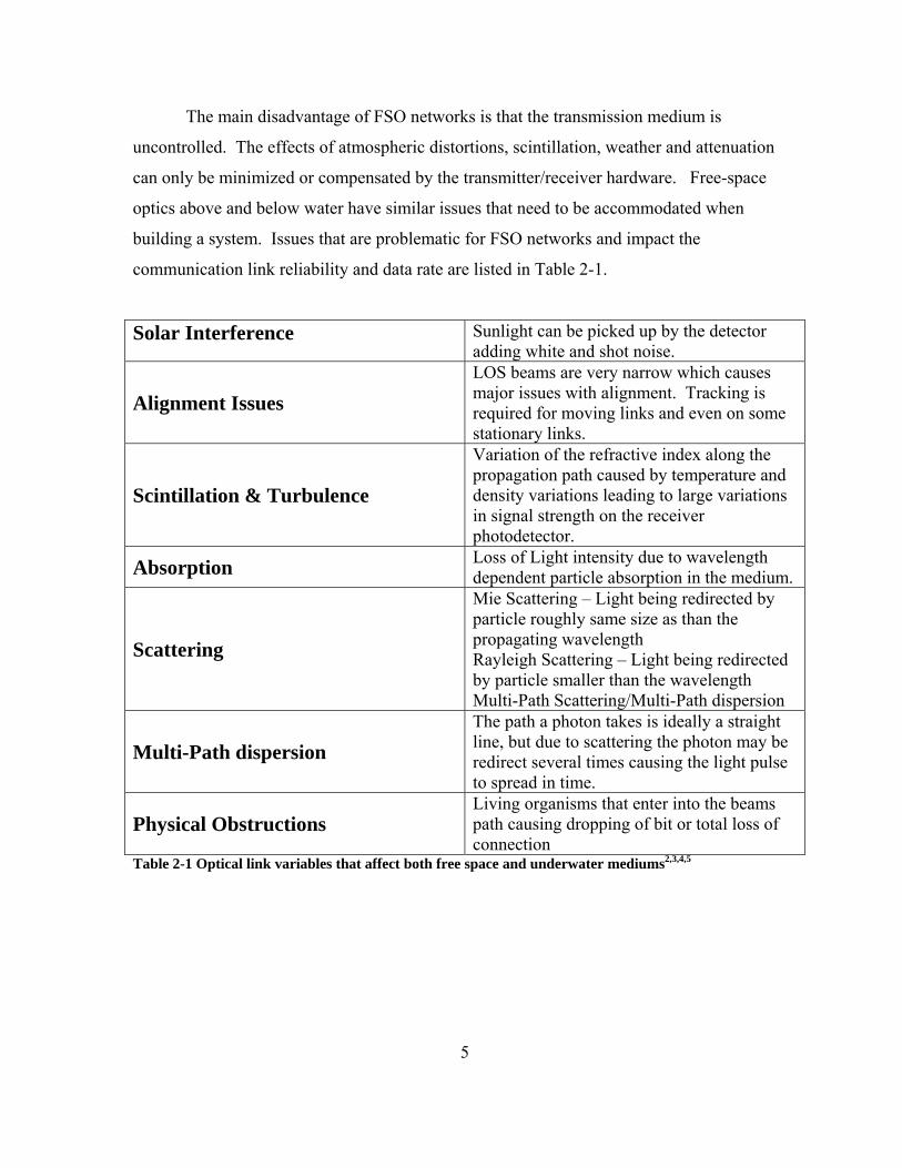
The main disadvantage of FSO networks is that the transmission medium is

uncontrolled. The effects of atmospheric distortions, scintillation, weather and attenuation

can only be minimized or compensated by the transmitter/receiver hardware. Free-space

optics above and below water have similar issues that need to be accommodated when

building a system. Issues that are problematic for FSO networks and impact the

communication link reliability and data rate are listed in Table 2-1.

Solar Interference Sunlight can be picked up by the detector adding white and shot noise.

Alignment Issues LOS beams are very narrow which causes major issues with alignment. Tracking is required for moving links and even on some stationary links.

Scintillation & Turbulence

Variation of the refractive index along the propagation path caused by temperature and density variations leading to large variations in signal strength on the receiver photodetector.

Absorption Loss of Light intensity due to wavelength dependent particle absorption in the medium.

Scattering

Mie Scattering – Light being redirected by particle roughly same size as than the propagating wavelength Rayleigh Scattering – Light being redirected by particle smaller than the wavelength Multi-Path Scattering/Multi-Path dispersion

Multi-Path dispersion The path a photon takes is ideally a straight line, but due to scattering the photon may be redirect several times causing the light pulse to spread in time.

Physical Obstructions Living organisms that enter into the beams path causing dropping of bit or total loss of connection

Table 2-1 Optical link variables that affect both free space and underwater mediums2,3,4,5

6

2.2 Appling FSO Concepts to Seawater

The transmitter and receiver for an underwater link can be very similar to a FSO link

in air, the major difference being the wavelength of operation. However, ocean water has

widely varying optical properties depending on location, time of day, organic and inorganic

content, as well as temporal variations such as turbulence. To construct an optical link it is

important to understand these properties. The loss of optical energy while traversing the link

arises from both absorption and scattering. Scattering also adversely impacts the link by

introducing multipath dispersion.

Water Types

The physical properties of ocean water vary both geographically, from the deep blue

ocean to littoral waters near land, and vertically with depth.

Vertically, the amount of light that is received from the sun is used to classify the

type of water. The topmost layer is called the

euphotic zone and is defined by how deeply

photosynthetic life can be found. Below this zone is

the dysphotic zone, sometimes as deeply as a

kilometer down, but the light is too faint to support

photosynthesis. From the lower boundary of this

zone and extending all the way to the bottom is the

aphotic zone, where no light ever passes and animals

have evolved to take advantage of other sources of

food7. Each zone has its own optical properties,

which adds another degree of difficulty when

constructing a link budget. A system in the euphotic

zone would act different than in the aphotic zone or

if it was going from zone to zone.

Figure 2-2 Diagram of the different oceanic zones, euphotic zone ends where 99% of the surface radiation has been absorbed, phytoplankton live and reproduce in this zone6.

7

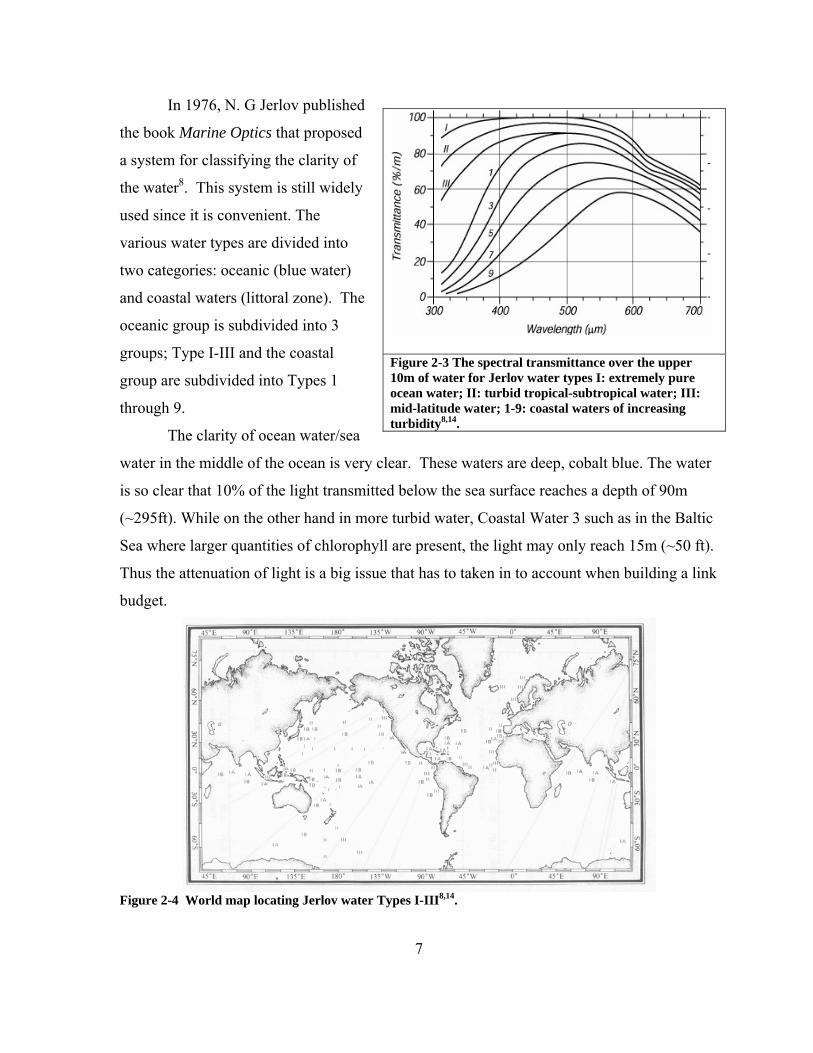
In 1976, N. G Jerlov published

the book Marine Optics that proposed

a system for classifying the clarity of

the water8. This system is still widely

used since it is convenient. The

various water types are divided into

two categories: oceanic (blue water)

and coastal waters (littoral zone). The

oceanic group is subdivided into 3

groups; Type I-III and the coastal

group are subdivided into Types 1

through 9.

The clarity of ocean water/sea

water in the middle of the ocean is very clear. These waters are deep, cobalt blue. The water

is so clear that 10% of the light transmitted below the sea surface reaches a depth of 90m

(~295ft). While on the other hand in more turbid water, Coastal Water 3 such as in the Baltic

Sea where larger quantities of chlorophyll are present, the light may only reach 15m (~50 ft).

Thus the attenuation of light is a big issue that has to taken in to account when building a link

budget.

Figure 2-4 World map locating Jerlov water Types I-III8,14.

Figure 2-3 The spectral transmittance over the upper 10m of water for Jerlov water types I: extremely pure ocean water; II: turbid tropical-subtropical water; III: mid-latitude water; 1-9: coastal waters of increasing turbidity8,14.

8

Fig. 2-4, is a map of the world showing different Jerlov water types are located.

Using this map we can estimate how an underwater platform might perform in different

locations, since the water type can be used to estimate the amount of chlorophyll

concentration hence the amount of absorption and scattering for a geographic location. With

satellite remote sensing technology, this map continues to change, but it employs a good

estimate for this research.

In the next section, the absorption and scattering properties of seawater will be

explained along with how the integration of the Jerlov water type classifications were use in

the calculations.

Attenuation Underwater

Attenuation underwater is the loss of beam intensity due to intrinsic absorption by

water, dissolved impurities, organic matter and scattering from the water, and impurities

including organic and inorganic particulate. The amount of attenuation changes with each

Jerlov water type. Each water type also contains different levels of biomass known as8,9:

• Phytoplankton-unicellular plants with light absorbing chlorophylls,

• Gelbstoffe -dissolved organic compounds know as yellow substance,

Other optical effects of the biomass include:

• Fluorescence -re-emission of light at a lower frequency by absorber

illuminated with optical energy,

• Bioluminescence- emission of light by marine organisms.

Bioluminescence does not actually absorb light, but various species of organisms release

light by there own means. The peak of the bioluminescent signals is centered on the blue-

green region and can potentially increase the noise present in the system.

9

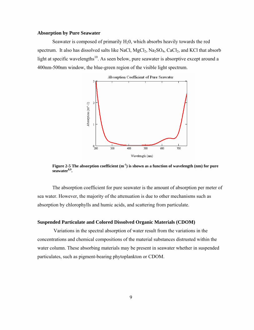
Absorption by Pure Seawater

Seawater is composed of primarily H20, which absorbs heavily towards the red

spectrum. It also has dissolved salts like NaCl, MgCl2, Na2SO4, CaCl2, and KCl that absorb

light at specific wavelengths10. As seen below, pure seawater is absorptive except around a

400nm-500nm window, the blue-green region of the visible light spectrum.

Figure 2-5 The absorption coefficient (m-1) is shown as a function of wavelength (nm) for pure seawater8,9.

The absorption coefficient for pure seawater is the amount of absorption per meter of

sea water. However, the majority of the attenuation is due to other mechanisms such as

absorption by chlorophylls and humic acids, and scattering from particulate.

Suspended Particulate and Colored Dissolved Organic Materials (CDOM)

Variations in the spectral absorption of water result from the variations in the

concentrations and chemical compositions of the material substances distrusted within the

water column. These absorbing materials may be present in seawater whether in suspended

particulates, such as pigment-bearing phytoplankton or CDOM.

10

Phytoplankton – Chlorophyll-a

Phytoplankton, derived from phyto, meaning plant and planktos, meaning wandering,

is one of the most influential factors in light transmission through ocean waters.

Phytoplankton live in the euphotic zone, which is the region from the surface to where only

1% of the sunlight reaches. Depending on the geographical location, time of day and season,

the zone ranges in depth from 50m to about 200m in open ocean; typically it’s around 100m7.

Phytoplankton use chlorophyll-a, which absorbs mostly in the blue and red region and

scatters green light to produce “food” through the process of photosynthesis10. As the

concentration of chlorophyll-a increases, more blue and red light are absorbed, leaving the

water a greenish tint.

Figure 2-6 Cubic spline curve fitting of the absorption coefficient as a function of chlorophyll concentrations in the different Jerlov water types11,9,12.

Another complicated factor with phytoplankton is its distribution within the euphotic

zone. Phytoplankton are not equally distributed vertically through the water column.

However they have been modeled assuming a Gaussian style distribution. The formula for

the depth profile for chlorophyll is13:

11

⎥⎦

⎤⎢⎣

⎡ −−++= 2

2max

2)(

exp2

*)(σπσzzhzSBzC o (Equation 2-1)

Where C(z) is the chlorophyll concentration (mg/m3) at depth z(m), Bo is the background

chlorophyll concentration at the sea surface (mg/m3), S is the vertical gradient of the

chlorophyll concentration (mg/m3/m), h is the total chlorophyll above the background

(mg/m2), σ, standard deviation of Gaussian distribution, controls the thickness of the

chlorophyll maximum layer (m), and zmax is the depth of the chlorophyll maximum (m)13.

This distribution described by Equation 2-1 , seen in Fig 2-7 , changes rapidly due to

temperature fluctuations and nutrients available in the water column. This is primarily due to

the changing of the seasons and the sun’s change in position in the sky. The areas around the

equator and the earth’s poles primarily stay the same due consistent temperatures and the

sun’s positioning. The eurphotic zone depth changes with each water type. The Jerlov Type I

water can be up to 200m and in Jerlov Coastal Region 9 it can be only 6m. This is because

the sun can only penetrate to a certain depth in each water case as shown in Fig 2-7.

Figure 2-7 Chlorophyll depth profile13, Right) Attenuation of surface irradiance with, Jerlov waters14,15.

12

Typically the position of the peak, zmax, moves closer to the top of the water column and the

magnitude of the peak concentration increases closer to land. The distribution of the

chlorophyll in deep ocean is more of a gradual slope.

Figure 2-8 In Type I-IB, there is a linear gradient without prominent peaks, in Type II-III, the chlorophyll maximum is in the subsurface layer, and in Type II-Coastal, the chlorophyll maximum is located at or near the sea surface13.

For the current link budget analysis, satellite remote sensing data, seen in the figure

below, and Figure 2-4 were used to estimate the chlorophyll concentration in the different

water types. The results from this analysis can be seen in Table 2-2.

13

Figure 2-9 Satellite remote sensor reading of the chlorophyll-a concentration over the entire globe [mg/m3]16 .

Jerlov Water Types Concentration of Chlorophyll mg/m^3

I 0.03 IA 0.1 IB .4 II 1.25 III 3

Coastal Water 1 9 Coastal Water 2 12

Table 2-2 Chlorophyll concentrations for different Jerlov Water types, take from Fig 2-4 and overlap with Fig 2-1016,8.

Color Dissolved Organic Material

CDOM, also know as gelbstoff (German for the word “yellow”), is composed of

decaying organic marine matter, which turns into humic and fulvic acids that absorb in the

blue region and fluoresce at 420-450nm17,9,18. Because blue is absorbed leaving green and

red, gelbstoff has a yellowish tint. Gelbstoff is generally present in low concentrations in

oceanic waters and in higher concentrations in the coastal waters8.

14

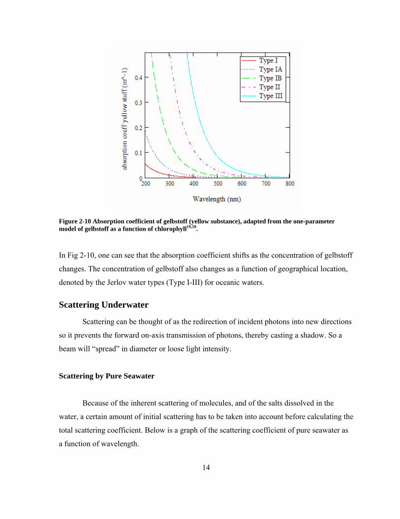
Figure 2-10 Absorption coefficient of gelbstoff (yellow substance), adapted from the one-parameter model of gelbstoff as a function of chlorophyll19,18.

In Fig 2-10, one can see that the absorption coefficient shifts as the concentration of gelbstoff

changes. The concentration of gelbstoff also changes as a function of geographical location,

denoted by the Jerlov water types (Type I-III) for oceanic waters.

Scattering Underwater

Scattering can be thought of as the redirection of incident photons into new directions

so it prevents the forward on-axis transmission of photons, thereby casting a shadow. So a

beam will “spread” in diameter or loose light intensity.

Scattering by Pure Seawater

Because of the inherent scattering of molecules, and of the salts dissolved in the

water, a certain amount of initial scattering has to be taken into account before calculating the

total scattering coefficient. Below is a graph of the scattering coefficient of pure seawater as

a function of wavelength.

15

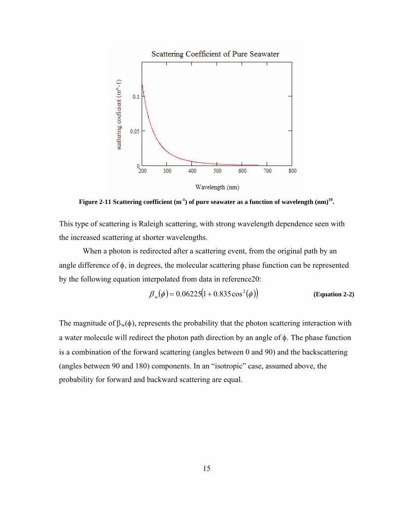
Figure 2-11 Scattering coefficient (m-1) of pure seawater as a function of wavelength (nm)19.

This type of scattering is Raleigh scattering, with strong wavelength dependence seen with

the increased scattering at shorter wavelengths.

When a photon is redirected after a scattering event, from the original path by an

angle difference of φ, in degrees, the molecular scattering phase function can be represented

by the following equation interpolated from data in reference20:

( ) ( )( )φφβ 2cos835.0106225.0 +=w (Equation 2-2)

The magnitude of βw(φ), represents the probability that the photon scattering interaction with

a water molecule will redirect the photon path direction by an angle of φ. The phase function

is a combination of the forward scattering (angles between 0 and 90) and the backscattering

(angles between 90 and 180) components. In an “isotropic” case, assumed above, the

probability for forward and backward scattering are equal.

16

0 50 100 150

0.1

Pure Seawater Scattering Phase Function

Scattering Angle (degrees)

Scat

terin

g ph

ase

func

tion

.15

0.06

B φ 1( )

1800 φ 1

Figure 2-12 The angular distribution of the scattering phase function for pure water20,12.

In an environment where there is scattering by particles, forward scattering will

dominate. This is true for example in clouds where the phase angle will typically be between

20 and 30 degrees, in the ocean the forward scattering angle will be around 7 degrees21,22.

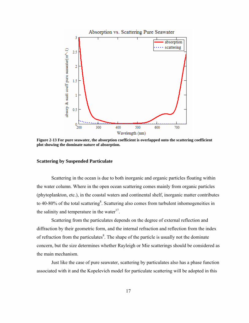
Although scattering plays a significant role in the lower wavelengths, when Fig. 2-11

is overlapped with Fig. 2-5, it is found that absorption dominates (Fig 2-13). For example, in

pure seawater attenuation is initially dominated by absorption. Closer to land where river

runoff introduce particulate and organic matter, scattering dominates the attenuation

coefficients. In turn it causes the minimum for attenuation to migrate from blue (~470nm) to

green (~550nm).

17

Figure 2-13 For pure seawater, the absorption coefficient is overlapped onto the scattering coefficient plot showing the dominate nature of absorption.

Scattering by Suspended Particulate

Scattering in the ocean is due to both inorganic and organic particles floating within

the water column. Where in the open ocean scattering comes mainly from organic particles

(phytoplankton, etc.), in the coastal waters and continental shelf, inorganic matter contributes

to 40-80% of the total scattering8. Scattering also comes from turbulent inhomogeneities in

the salinity and temperature in the water17.

Scattering from the particulates depends on the degree of external reflection and

diffraction by their geometric form, and the internal refraction and reflection from the index

of refraction from the particulates8. The shape of the particle is usually not the dominate

concern, but the size determines whether Rayleigh or Mie scatterings should be considered as

the main mechanism.

Just like the case of pure seawater, scattering by particulates also has a phase function

associated with it and the Kopelevich model for particulate scattering will be adopted in this

18

work. For this model, the total scattering function is a linear combination of the phase

function ρs, describing the scattering by small particles and ρl, describing the scattering by

large particles associates with biogenic fraction of marine hydrosol (phytoplankton)19. This

gives us the total hydrosol angular scattering coefficient:

( ) ( ) ( ) ( ) ( ) llols

osHy CbCb ****, φρλφρλφλβ += (Equation 2-3)

Where the small particle phase and large particle phase function are expressed as ρs(φ) and

ρl(φ), respectively and φ is the scattering angle in degrees19:

⎥⎦

⎤⎢⎣

⎡= ∑

=

5

1

43

exp*61746.5)(n

n

ns s φφρ , ⎥⎦

⎤⎢⎣

⎡= ∑

=

5

1

43

exp*381.188)(n

n

nl l φφρ (Equation 2-4)

The coefficients sn and ln are given in Table below: n 1 2 3 4 5

sn -2.957089*10-2 -2.782943*10-2 1.255406*10-3 -2.155880*10-5 1.356632*10-7

ln -1.604327 8.157686*10-2 -2.150389*10-3 2.419323*10-5 -6.578550*10-8

Table 2-3 Small and Large particle coefficients for the hydrosol angular phase function19.

The seawater angular scattering coefficient is the linear combination of a Rayleigh phase

function of scattering, ρr, and the hydrosol phase functions ρs and ρl. This gives us19:

( ) ( )φφρ 2cos6531.07823.0 +=r (Equation 2-5)

( ) ( ) ( ) ( ) ( ) ( ) ( ) llolss

osroH CbCbb ****, φρλφρλφρλφλβ ++= (Equation 2-6)

19

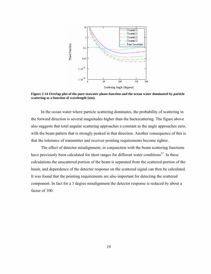
Figure 2-14 Overlap plot of the pure seawater phase function and the ocean water dominated by particle scattering as a function of wavelength (nm).

In the ocean water where particle scattering dominates, the probability of scattering in

the forward direction is several magnitudes higher than the backscattering. The figure above

also suggests that total angular scattering approaches a constant as the angle approaches zero,

with the beam pattern that is strongly peaked in that direction. Another consequence of this is

that the tolerance of transmitter and receiver pointing requirements become tighter.

The effect of detector misalignment, in conjunction with the beam scattering functions

have previously been calculated for short ranges for different water conditions23. In these

calculations the unscattered portion of the beam is separated from the scattered portion of the

beam, and dependence of the detector response on the scattered signal can then be calculated.

It was found that the pointing requirements are also important for detecting the scattered

component. In fact for a 3 degree misalignment the detector response is reduced by about a

factor of 100.

20

Figure 2-15 Influence of detector angle with respect to the beam axis for scattered photons. Data is from calculations from reference 23 . Note that this assumes that the detector is on the beam axis. If the detector is placed off axis the detector response will be further reduced.

Turbulence For the purposes of this study, scintillation from turbulent water, variations of the

refractive index due to variations from flow, salinity, and temperature and effects of stratified

layers of water are ignored since they are considered to be less important than absorption and

scattering. However they can be expected to have significant second order effects, some of

which are briefly outlined below.

The refractive index of seawater and it dependence on environmental parameters has

been measured24. Water is relatively incompressible, however with increasing depth and

pressure the refractive index increases. This change is relatively small with the increase of

about 1.37x10-4 for 100 meters depth. The temperature dependence on the refractive index is

near a maximum of 4 oC at about 1.334 and decreases with temperature to about 1.3319 at 30 oC. The impact of salinity is larger still with one part per thousand increase in salinity (1

gr/kilogram) resulting in 1.92x10-4 increase in refractive index. The highest expected salinity

in sea water is roughly ~40 g/kg, while the least is ~ 5 g/kg for artic water with a lot of ice

melt. Which may seem like small index changes but for long optical path lengths gradients in

21

could the refractive index can result in significant deflections of an optical beam. While these

effects can be expected to increase the difficulty of pointing and tracking between

underwater platforms, since the expected ranges are relatively short and these effects are

expected to be secondary problems compared to scattering and attenuation. These effects also

will be more prominent when the optical path is not horizontal or vertical. These effects limit

the pointing & tracking between underwater links, however due to the relatively short range

they are of secondary order compared to scattering and attenuation, although they could be

more prominent when the optical path is not horizontal or vertical.

A model of the scintillation due to turbulence in the water was not developed, but is

expected to be important. It is not clear from the literature the magnitude of the effects. The

variations in refractive index are higher due to the increased density of the medium; however

the viscosity of the medium is also much higher, damping the size of turbulence cells

expected. Thus the length scales of the turbulence are typically much smaller. The impact of

the turbulence is also influenced by the coherence length of the light source used. For LED

light sources the scintillation of the light source by turbulence will be mitigated. Similarly the

effects of currents and other flow related phenomena that could impact the propagation of

light between platforms. Flow over the transmitter and receiver apertures can also be

expected to have effects due to the changes in density due to the flow. Ideally the position of

the apertures should be placed where the flow is laminar, and turbulence from protrusions is

not significant.

In Chapter 3, all the inherent optical properties will be used to build a theoretical

power link budget for an underwater optical communications link traveling in the horizontal

direction.

22

2.3 References

1 S. G. Lambert, W. L. Casey, Laser Communications in Space, Artech House Publishers, Boston, (1995) 2 G. Keiser, “Optical Fiber Communications” McGraw-Hill Higher Education, 3rd Edition, pg 94-100, (2000) 3 J. C. Palais, Fiber Optic Communications, 4th Edition Prentice Hall, New Jersey, pg 109-115,(1998) 4 S. Bloom, E. Korevaar, J. Schuster, H. Willerbrand, Understanding the performance of free-space optics.” Journal of Optical Networking, Vol. 2, No. 6, (June 2003) 5 J. Ricklin, A. Mujumdar, SC656 Fundamentals of Free-space Laser communications, SPIE Education Sevices Short Course Notes, Optical Science and Technology, the SPIE 49th Annual Meeting ,2-6 (August 2004) Denver CO 6 Picture from http://www.aquatic.uoguelph.ca/oceans/Introduction/Zonation/zonation.htm 7 Tom Garrison, Oceanography: An invitation to Marine Science, Chapter 10, Wadsworth Publishing Company, Belmont, (1996) 8 J. R. Apel, Principles of Ocean Physic, pp509-584, International Geophysics Series, Vol. 38, Academic Press, (1987) 9 H. Arst, Optical Properties and Remote Sensing of Multicomponental Water Bodies, Praxis Publishing, Chichester, UK, pg 8-28, (2003) 10 K.S. Shifrin, Physical Optics of Ocean Water, American Institute of Physics, New York, pg 18-22, 70-77, (1983) 11 C.S. Yentsch, “The Influence of Phytoplankton Pigments on the Color of Sea Water”, Deep-Sea Res., 7, 1, (1960). 12 Excerpted from: Ocean Optics Protocols for Satellite Ocean Color Sensor Validation, Chapter 1 Sections 2 & 3, Rev 4, Volume IV 13 T. Kameda, S. Matsumura, “Chlorophyll Biomass off Sanriku, Northwestern Pacific, Estimated by Ocean Color and Temperature Scanner (OCTS) and a Vertical Distribution Model,”, National Research Institute of Far Seas Fisheries, Orido 5-7-1, Shimizu, Shizuoka 424-8633, Japan, (1998)

23

14 N.G. Jerlov, Optical Oceanography, Elsevier Publishing Company, New York, Vol. 5, pg 50-62, 118-126, (1968) 15 K.S Shifrin, Physical Optics of Ocean Water, American Institute of Physics, New York, (1988) 16 Picture found at http://www.marktechopto.com/engineering/history.cfm 17 Waiebke Breves, Rainer Teuter. “Bio-optical properties of gelbstoff in the Arabian Sea at the onset of the southwest monsoon”, Earth Planet Science, 109, No. 4 Dec 2000. 18 D.A. Hansell, C.A. Carlson, Biogeochemistry of Marine Dissolved Organic Mater, Academic Press, New York, pg 509-534, (2002) 19 V.I. Haltrin, Chlorophyll-based model of seawater optical properties, Appl. Opt.,38,No.33, (Nov 1999) 20 A. Morel, Optical properties of pure water and pure sea water, in Optical Aspects of Oceanography, edited by N. G. Jerlov and E. S. Nielsen, Academic Press, New York, USA, (1974). 21 E.A. Buchner, “Computer Simulation of Light Pulse Propagation for Communication Through Thick Clouds”, Applied Optics, 12, 2391 (1973) and E.A. Buchner and R.M. Lerner, “Experiments on LightPulse Communication and Propagation Through Atmospheric Clouds” Appl. Opt. 12, 2401 (1973) 22 J.W. Mclean, J.D. Freeman, R.E. Walker, “Beam Spread Function with Time Dispersion”, Applied Optics, 37 4701, (1998) 23 R. Sanchez and N. J. McCormick, “Analytic beam spread function for ocean optics applications” Applied Optic, 41, 6276 (2002) 24 X. Quan, E. S. Fry, "Empirical equation for the index of refraction of seawater," Appl. Opt.,34, 3477- 3480 (1995).

24

Chapter 3 Link Budget

Judging the relative merits of optical communication systems can be difficult due to

the wide variety of different methods that can be used to communicate. The usual method of

comparing the relative merits of communication systems is to use Bit-rate Length product.

This FOM has been used to discuss the evolution of communications systems, especially the

fiber optic communication systems.

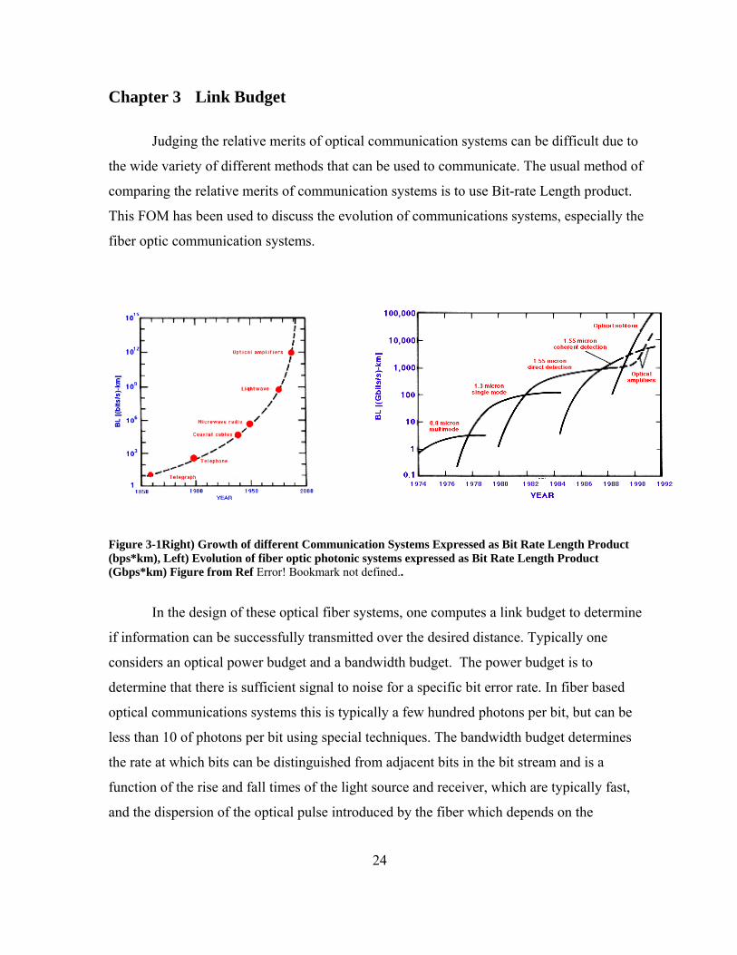
Figure 3-1Right) Growth of different Communication Systems Expressed as Bit Rate Length Product (bps*km), Left) Evolution of fiber optic photonic systems expressed as Bit Rate Length Product (Gbps*km) Figure from Ref Error! Bookmark not defined..

In the design of these optical fiber systems, one computes a link budget to determine

if information can be successfully transmitted over the desired distance. Typically one

considers an optical power budget and a bandwidth budget. The power budget is to

determine that there is sufficient signal to noise for a specific bit error rate. In fiber based

optical communications systems this is typically a few hundred photons per bit, but can be

less than 10 of photons per bit using special techniques. The bandwidth budget determines

the rate at which bits can be distinguished from adjacent bits in the bit stream and is a

function of the rise and fall times of the light source and receiver, which are typically fast,

and the dispersion of the optical pulse introduced by the fiber which depends on the

25

information channel. Typically the dispersion of the information channel is the limiting

factor of the bandwidth budget.

Power Budget

Assuming a specific wavelength of operation, and a goal of a specific Bit Error Rate

(BER) to construct the power budget for a simple point to point link, one should consider:

• The transmitter output power,

• Coupling efficiency of the source and receiver to the fiber,

• Attenuation or loss of optical energy due to scattering, or absorption in

(dB/km)

• Losses due to fiber splices, and

• Receiver sensitivity typically expressed in dB (or sometimes bit-rate/mW).

• System margin, typically about 6 dB to account for system component ageing.

If the transmitter power minus the sum of the losses is greater than the sum of the

receiver sensitivity plus the system margin for a given wavelength and bit error rate, the link

should be successful1.

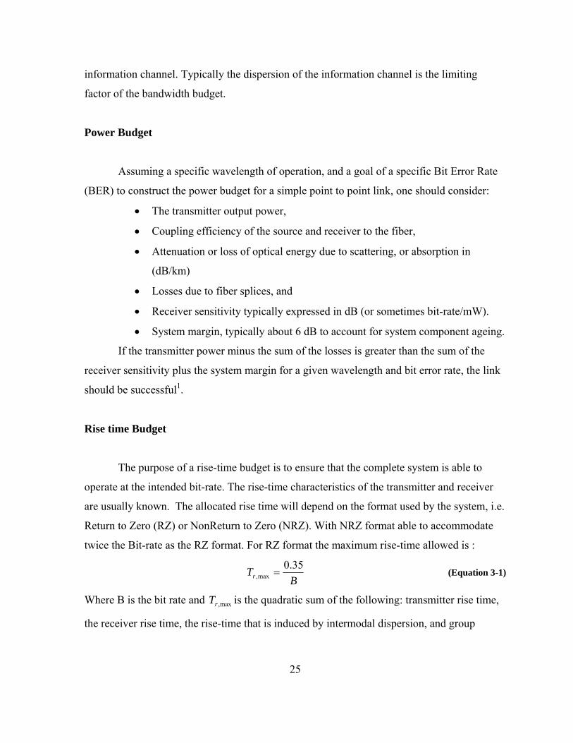
Rise time Budget

The purpose of a rise-time budget is to ensure that the complete system is able to

operate at the intended bit-rate. The rise-time characteristics of the transmitter and receiver

are usually known. The allocated rise time will depend on the format used by the system, i.e.

Return to Zero (RZ) or NonReturn to Zero (NRZ). With NRZ format able to accommodate

twice the Bit-rate as the RZ format. For RZ format the maximum rise-time allowed is :

B

Tr35.0

max, = (Equation 3-1)

Where B is the bit rate and max,rT is the quadratic sum of the following: transmitter rise time,

the receiver rise time, the rise-time that is induced by intermodal dispersion, and group

26

velocity dispersion caused by the fiber. The 0.35 comes from the assumption that a RC-low

frequency band pass model can be used to describe the response of the system to an impulse.

The dispersion, the spread of the optical pulse in time is expressed in ps/nm-km for

chromatic dispersion or ps/km for modal or multipath dispersion. In single mode fibers,

chromatic dispersion dominates while for multimode fiber systems the modal dispersion

dominates1.

Depending on the choice of components, the system will be either attenuation or

dispersion limited as shown in the graph below. Similarly it will be important for underwater

communications to consider when underwater link will be limited by multipath dispersion

from scattering and when it is power limited.

Figure 3-2 The limits of system performance can be shown graphically by plotting maximum ling length vs Bit rate. Above the horizontal portion of the curves, the systems are photon limited. To the right, the systems are dispersion limited. Note that the dispersion limit is particularly severe for multimode step index fibers. In underwater optical communication systems dispersion can also be expected to play a significant role. Figure after data from Ref. 2.

In the underwater scenario the rise time due to scattering will be important at high data

rates. To date there doesn’t appear to be any measured data for communication systems

underwater that have measure the effects on scattering on dispersion.

27

3.1 Computing Free Space Link Budgets

The principal difference between optical fiber based communication systems and the other communications systems is that the characteristics of the optical fiber are so well defined. In free space systems, interactions with the environment dominate both in terms of geometric effects such as the beam expanding due to diffraction or absorption and scattering.

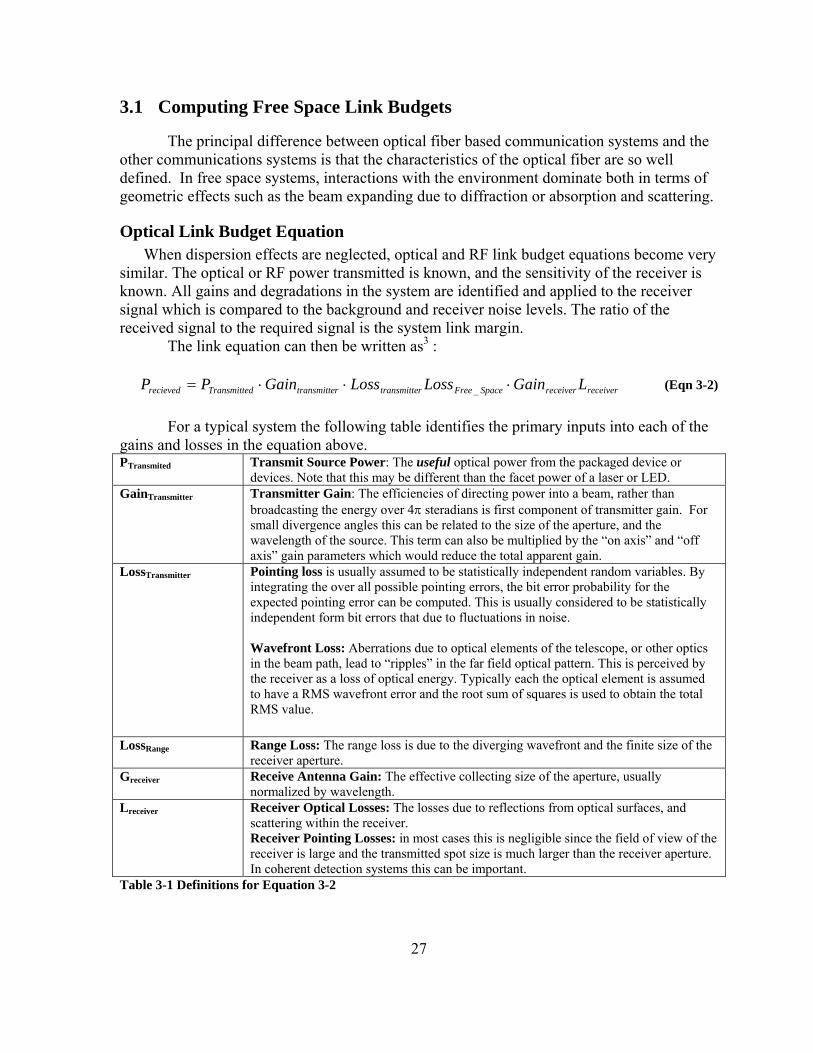
Optical Link Budget Equation When dispersion effects are neglected, optical and RF link budget equations become very

similar. The optical or RF power transmitted is known, and the sensitivity of the receiver is known. All gains and degradations in the system are identified and applied to the receiver signal which is compared to the background and receiver noise levels. The ratio of the received signal to the required signal is the system link margin.

The link equation can then be written as3 :

receiverreceiverSpaceFreertransmittertransmittedTransmitterecieved LGainLossLossGainPP ⋅⋅⋅= _ (Eqn 3-2)

For a typical system the following table identifies the primary inputs into each of the gains and losses in the equation above. PTransmited Transmit Source Power: The useful optical power from the packaged device or

devices. Note that this may be different than the facet power of a laser or LED. GainTransmitter Transmitter Gain: The efficiencies of directing power into a beam, rather than

broadcasting the energy over 4π steradians is first component of transmitter gain. For small divergence angles this can be related to the size of the aperture, and the wavelength of the source. This term can also be multiplied by the “on axis” and “off axis” gain parameters which would reduce the total apparent gain.

LossTransmitter Pointing loss is usually assumed to be statistically independent random variables. By integrating the over all possible pointing errors, the bit error probability for the expected pointing error can be computed. This is usually considered to be statistically independent form bit errors that due to fluctuations in noise. Wavefront Loss: Aberrations due to optical elements of the telescope, or other optics in the beam path, lead to “ripples” in the far field optical pattern. This is perceived by the receiver as a loss of optical energy. Typically each the optical element is assumed to have a RMS wavefront error and the root sum of squares is used to obtain the total RMS value.

LossRange Range Loss: The range loss is due to the diverging wavefront and the finite size of the receiver aperture.

Greceiver Receive Antenna Gain: The effective collecting size of the aperture, usually normalized by wavelength.

Lreceiver Receiver Optical Losses: The losses due to reflections from optical surfaces, and scattering within the receiver. Receiver Pointing Losses: in most cases this is negligible since the field of view of the receiver is large and the transmitted spot size is much larger than the receiver aperture. In coherent detection systems this can be important.

Table 3-1 Definitions for Equation 3-2

28

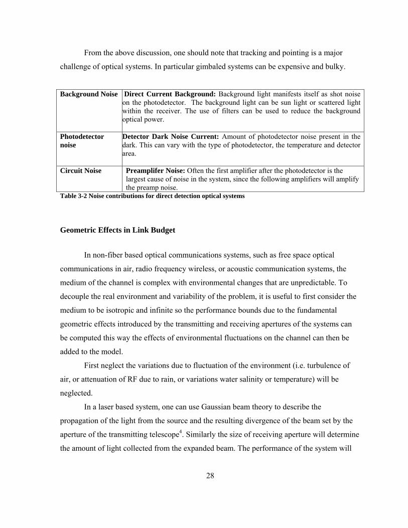
From the above discussion, one should note that tracking and pointing is a major

challenge of optical systems. In particular gimbaled systems can be expensive and bulky.

Background Noise Direct Current Background: Background light manifests itself as shot noise on the photodetector. The background light can be sun light or scattered light within the receiver. The use of filters can be used to reduce the background optical power.

Photodetector noise

Detector Dark Noise Current: Amount of photodetector noise present in the dark. This can vary with the type of photodetector, the temperature and detector area.

Circuit Noise Preamplifer Noise: Often the first amplifier after the photodetector is the largest cause of noise in the system, since the following amplifiers will amplify the preamp noise.

Table 3-2 Noise contributions for direct detection optical systems

Geometric Effects in Link Budget

In non-fiber based optical communications systems, such as free space optical

communications in air, radio frequency wireless, or acoustic communication systems, the

medium of the channel is complex with environmental changes that are unpredictable. To

decouple the real environment and variability of the problem, it is useful to first consider the

medium to be isotropic and infinite so the performance bounds due to the fundamental

geometric effects introduced by the transmitting and receiving apertures of the systems can

be computed this way the effects of environmental fluctuations on the channel can then be

added to the model.

First neglect the variations due to fluctuation of the environment (i.e. turbulence of

air, or attenuation of RF due to rain, or variations water salinity or temperature) will be

neglected.

In a laser based system, one can use Gaussian beam theory to describe the

propagation of the light from the source and the resulting divergence of the beam set by the

aperture of the transmitting telescope4. Similarly the size of receiving aperture will determine

the amount of light collected from the expanded beam. The performance of the system will

29

then be determined by the pointing accuracies and tracking ability of the transmitter and

receiver. Similarly for LED based systems, the performance will be determined by geometric

effects determined by the divergence of the beam (substantially greater than that of the laser)

and size of the receiving apertures. One can equivalently discuss these geometric effects in

terms of antenna theory and optical cross-sections. This can be especially useful when

comparing optical systems with pulsed RF systems such as radars. Typically for optical free

space communications over substantial distances multi-path, or multiple bounces off light the

environment, are not considered since such bounces tend diffuse reflections.

Environmental Consideration in Link Budgets

Significant efforts have been made in trying to understand what is required for a

reliable link for free space optical communications in air and space. As mentioned above, the

geometric effects are fairly straightforward to compute. However, transmission through the

atmosphere poses special problems. In addition to water vapor and CO2 absorption, and

scattering by aerosol particles, the atmosphere has a structure that varies with altitude.

Visibility a useful way to evaluate the suitability of the atmosphere and can range

from a couple of hundred meters in fog or snow to tens of kilometers in the upper atmosphere

on a clear day.

The atmosphere is also turbulent with the amount depending on the local

environmental conditions. The hot earth typically creates significant turbulence near the

surface. Usually the turbulence is modeled as convection cells with a length scale depending

on the conditions. Each cell is then treated as having a locally homogeneous and isotropic

index of refraction. Since the speed of light is so fast, one can then consider the atmosphere

frozen for each particular instant in time and to remain relatively constant over time periods

of a few milliseconds. The time scale changes of the atmosphere are slow enough that

adaptive optics can be used to correct for the effects of turbulence. However in general one

should keep in mind that sending a laser horizontally through the atmosphere near the surface

of the earth can be quite different than sending the beam vertically. The length scale of the

turbulence can typically be bounded by a short and long length scale. Usually a turbulence

30

strength parameter Cn2 is used to get a statistical measure of the refractive index

fluctuations5,6.

In general, received power is of most importance, or the integrated intensity divided

by the area of the detector. The spatial and temporal variations in the atmosphere lead to

variations in the irradiance of the received beam which is perceived as scintillation. One

effect of the scintillation is that one instant the received signal is extremely strong due to

constructive scattering and interference effects, but at another instant may be negligible.

These effects can be summarized as quoted from reference 3 below:

• Beam Steering - Angular deviation of the beam from the line-of-sight path, causing

the beam to miss the receiver.

• Image Dancing – Variations in the beam arrival angle, causing the focus point to

move in the image plane.

• Beam Spreading – small angle scattering, increasing the beam divergence and

causing a decrease of the spatial power density at the receiver.

• Beam Scintillation – small scale destructive interferences within the beam cross-

section, causing variations in the spatial power density at the receiver.

• Spatial Coherence Degradation – losses in phase coherence across the beam phase

fronts, degrading the photo-mixing performance

• Polarization Fluctuations – fluctuations in the polarization state.

The background irradiance due to sunlight can also be a major consideration. It obviously

varies with time of day, and in the underwater systems is strongly dependent on the direction

of the receiver aperture and the water depth.

FSO Power Link Budget Equation

The basic formula for a typical optical link is an exponential decaying function as function

of the path length L, Beer’s Law:

31

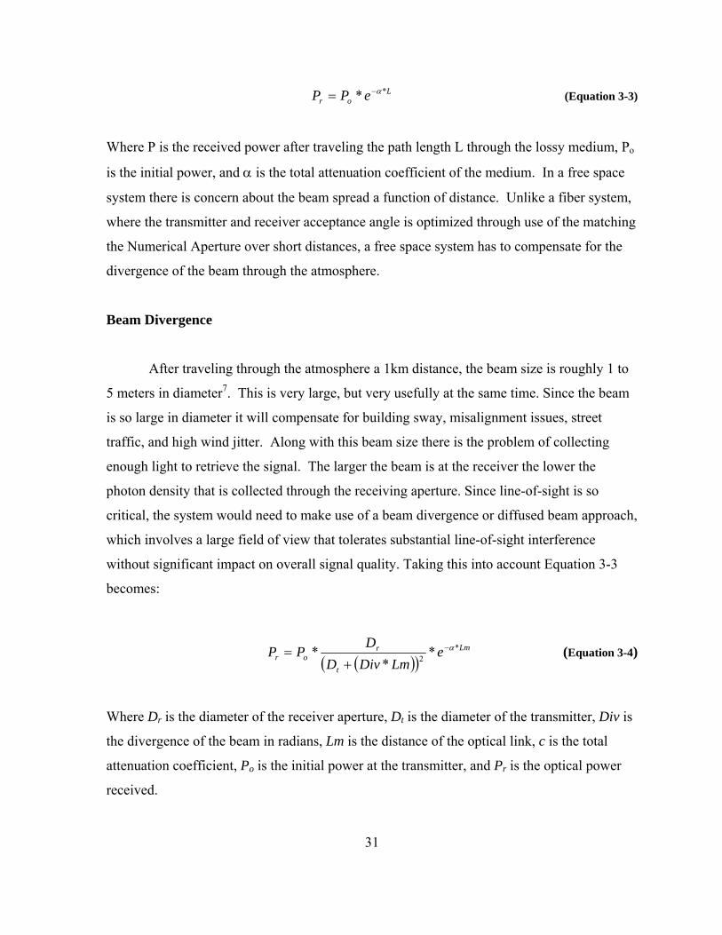
Lor ePP ** α−= (Equation 3-3)

Where P is the received power after traveling the path length L through the lossy medium, Po

is the initial power, and α is the total attenuation coefficient of the medium. In a free space

system there is concern about the beam spread a function of distance. Unlike a fiber system,

where the transmitter and receiver acceptance angle is optimized through use of the matching

the Numerical Aperture over short distances, a free space system has to compensate for the

divergence of the beam through the atmosphere.

Beam Divergence

After traveling through the atmosphere a 1km distance, the beam size is roughly 1 to

5 meters in diameter7. This is very large, but very usefully at the same time. Since the beam

is so large in diameter it will compensate for building sway, misalignment issues, street

traffic, and high wind jitter. Along with this beam size there is the problem of collecting

enough light to retrieve the signal. The larger the beam is at the receiver the lower the

photon density that is collected through the receiving aperture. Since line-of-sight is so

critical, the system would need to make use of a beam divergence or diffused beam approach,

which involves a large field of view that tolerates substantial line-of-sight interference

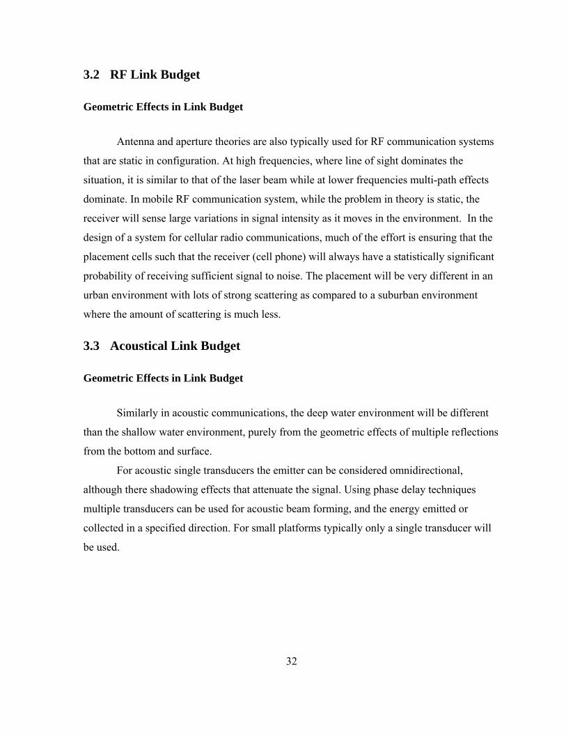
without significant impact on overall signal quality. Taking this into account Equation 3-3

becomes:

( )( )Lm

t

ror e

LmDivDDPP *

2 **

* α−

+= (Equation 3-4)

Where Dr is the diameter of the receiver aperture, Dt is the diameter of the transmitter, Div is

the divergence of the beam in radians, Lm is the distance of the optical link, c is the total

attenuation coefficient, Po is the initial power at the transmitter, and Pr is the optical power

received.

32

3.2 RF Link Budget

Geometric Effects in Link Budget

Antenna and aperture theories are also typically used for RF communication systems

that are static in configuration. At high frequencies, where line of sight dominates the

situation, it is similar to that of the laser beam while at lower frequencies multi-path effects

dominate. In mobile RF communication system, while the problem in theory is static, the

receiver will sense large variations in signal intensity as it moves in the environment. In the

design of a system for cellular radio communications, much of the effort is ensuring that the

placement cells such that the receiver (cell phone) will always have a statistically significant

probability of receiving sufficient signal to noise. The placement will be very different in an

urban environment with lots of strong scattering as compared to a suburban environment

where the amount of scattering is much less.

3.3 Acoustical Link Budget

Geometric Effects in Link Budget

Similarly in acoustic communications, the deep water environment will be different

than the shallow water environment, purely from the geometric effects of multiple reflections

from the bottom and surface.

For acoustic single transducers the emitter can be considered omnidirectional,

although there shadowing effects that attenuate the signal. Using phase delay techniques

multiple transducers can be used for acoustic beam forming, and the energy emitted or

collected in a specified direction. For small platforms typically only a single transducer will

be used.

33

Environmental Consideration in Link Budgets

In an acoustical communication system, transmission loss is caused by energy

spreading and sound absorption. Energy spreading loss depends only on the propagation

distance, but the absorption loss increases with range and frequency. Just like other links,

these problems set the limit on the available bandwidth.

Link condition is largely influenced by the spatial varying condition of the

underwater acoustic channel. Acting like a waveguide, the seabed and the air/water interface.

Various phenomena, including formation of the shadow zones, evolve from this variation.

Transmission loss at a particular location can be predicted by many of the propagation

modeling techniques with various degrees of accuracy. Spatial dependence of transmission

loss imposes severe problems for mobile communication systems with both the transmitter

and receiver moving.

Noise observed in the ocean exhibits strong frequency dependence as well as location

dependence. Generally the inshore environments, such as marine work-sites, are much

noisier than the deep ocean due to the man-made noise. Most of the ambient noise sources

can be described as having a continuous spectrum and Gaussian statistics. As an

approximation, the ambient noise power spectral density is commonly assumed to decay at

20 dB/decade, both in shallow and deep water, over frequencies which are of interest to

communication systems design8.

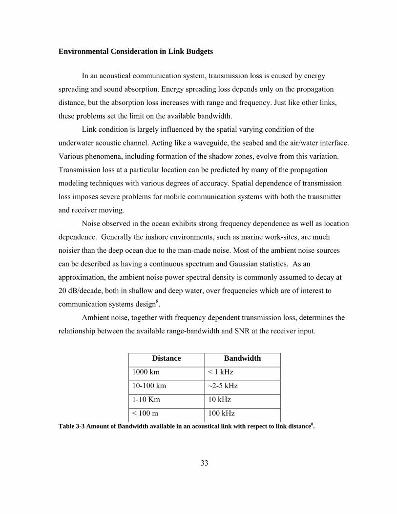
Ambient noise, together with frequency dependent transmission loss, determines the

relationship between the available range-bandwidth and SNR at the receiver input.

Distance Bandwidth

1000 km < 1 kHz

10-100 km ~2-5 kHz

1-10 Km 10 kHz

< 100 m 100 kHz Table 3-3 Amount of Bandwidth available in an acoustical link with respect to link distance8.

34

Within this limited bandwidth, the signal is subject to multi-path propagation through

a channel whose characteristics varies with time and is highly dependent on the location of

the transmitter and receiver. The multi-path structure depends on the link configuration,

which is primarily designated as vertical or horizontal. The vertical channels exhibit little

multi-path, but the horizontal channels are subject to larger amounts multi-path spreads.

Multi-path propagation causes severe degradation of the acoustic communication signals.

Combating the underwater multi-path to achieve a high data throughput is the most

challenging task of an underwater acoustic communication system8.

3.4 Underwater Optical Link Budget

Many factors must be considered when calculating a “true” link budget; Weather,

wavelength of the laser, distance of the link, underwater currents, scattering, misalignment,

attenuation, absorption, and data rates are just a few of the things that must be considered.

Other factors such as the light source (laser, LED), detector (PIN, APD), and other bottle-

neck electronics must also be considered.

Geometric Effects in Link Budget

In the underwater environment especially in turbid water scattering can be expected

to be the dominate effect. In addition to attenuating the signal, the scattering can also be

viewed as strongly influencing the transverse intensity of the beam profile. This can also

result in very stringent pointing requirements since the percentage of forward scattered light

will be strongly peaked at small angles.

Building an Underwater Link Model

The main motivation as the topic for this thesis was to research the possibility of

using semiconductor light sources as a mean to communicate underwater. However, as

described above, scattering and the variable optical qualities of ocean water need to be

considered. These varying properties change with time and location which in turn could

affect the amount of light lost. This could also cause a shift in the appropriate operating

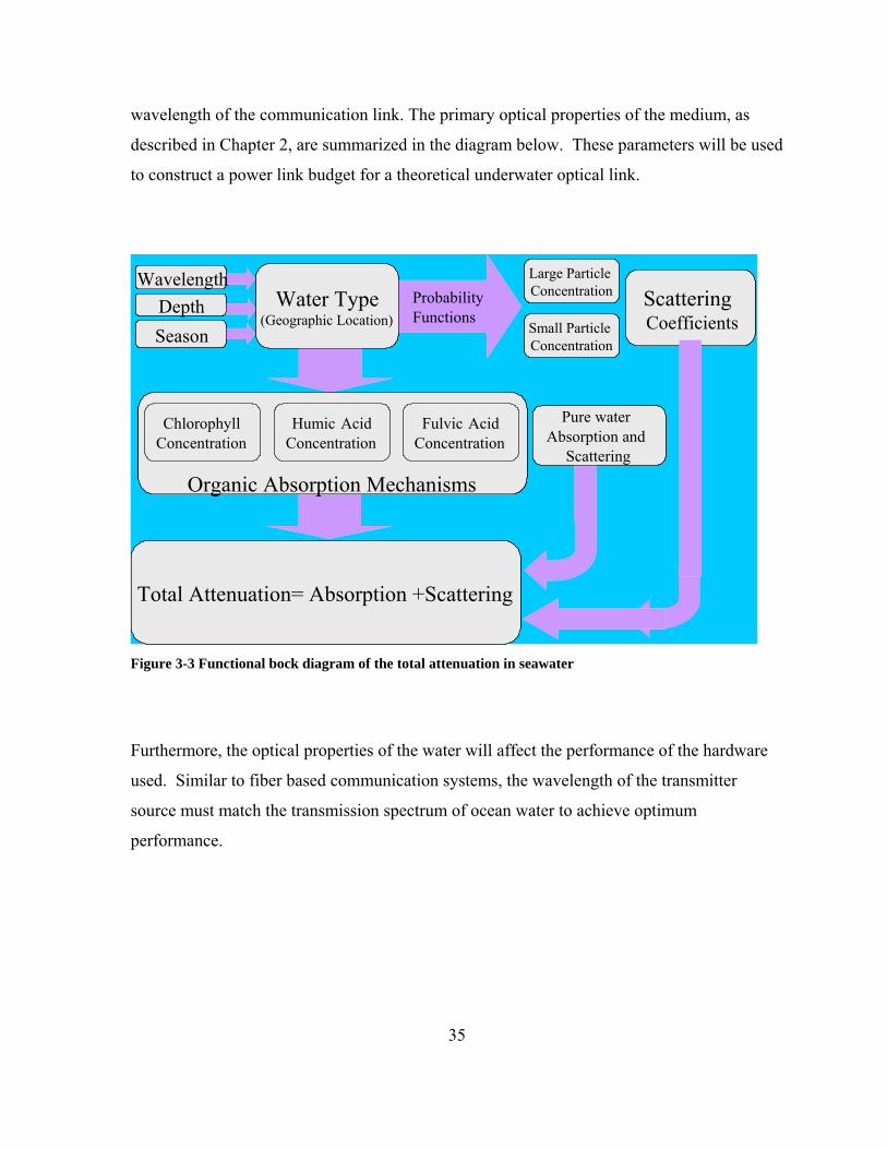
35

wavelength of the communication link. The primary optical properties of the medium, as

described in Chapter 2, are summarized in the diagram below. These parameters will be used

to construct a power link budget for a theoretical underwater optical link.

Figure 3-3 Functional bock diagram of the total attenuation in seawater

Furthermore, the optical properties of the water will affect the performance of the hardware

used. Similar to fiber based communication systems, the wavelength of the transmitter

source must match the transmission spectrum of ocean water to achieve optimum

performance.

Probability Functions

Water Type(Geographic Location)

SeasonDepth

WavelengthScattering Coefficients

Organic Absorption Mechanisms

ChlorophyllConcentration

Humic AcidConcentration

Fulvic AcidConcentration

Total Attenuation= Absorption +Scattering

Pure water Absorption and

Scattering

Probability Functions

Water Type(Geographic Location)

SeasonDepth

WavelengthScattering Coefficients

Large Particle Concentration

Small Particle Concentration

Organic Absorption Mechanisms

ChlorophyllConcentration

Humic AcidConcentration

Fulvic AcidConcentration

Organic Absorption Mechanisms

ChlorophyllConcentration

Humic AcidConcentration

Fulvic AcidConcentration

Total Attenuation= Absorption +Scattering

Pure water Absorption and

Scattering

36

Figure 3-4 Absorption spectrum of clear ocean water, showing that InGaN light emitters match the optical transmission window of sea water.

In addition to the optical parameters in Figure 3-3, the receiver and transmitter inputs are

now considered when building a comprehensive model of the optical performance of the link.

TX LENS

Output PowerRise Time

Beam Divergence

Current DrawVoltage Supply

Line WidthPointing Loss

LENSFilter RXAnti

ReflecCoat

Quantum EfficiencyOptical ResponsivelyArea of Photojunction

Rise TimePointing LossNoise – Temp Shot Solar

Water TypeRangeDepth

SeasonWavelength

Chlorophyll ConcentrationHumic Acid ConcentrationFulvic Acid Concentration

Large Particle ConcentrationSmall Particle Concentration

Index of RefractionScattering Coeff Large ParticlesScattering Coeff Small Particles

Scattering Coeff Pure WaterAbsorption Coeff ChlorophyllAbsorption Coeff Humic AcidAbsorption Coeff Fulvic AcidAbsorption Coeff Pure Water

Medium InputsTransmitter

InputsReciever Inputs

Figure 3-5 Block Diagram summarizing all the variable needing consideration in the Link Budget.

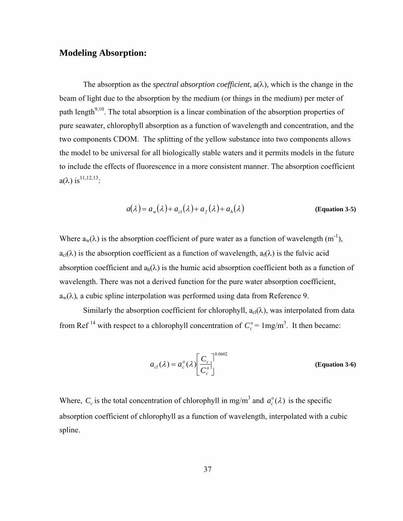
37

Modeling Absorption:

The absorption as the spectral absorption coefficient, a(λ), which is the change in the

beam of light due to the absorption by the medium (or things in the medium) per meter of

path length9,10. The total absorption is a linear combination of the absorption properties of

pure seawater, chlorophyll absorption as a function of wavelength and concentration, and the

two components CDOM. The splitting of the yellow substance into two components allows

the model to be universal for all biologically stable waters and it permits models in the future

to include the effects of fluorescence in a more consistent manner. The absorption coefficient

a(λ) is11,12,13:

( ) ( ) ( ) ( ) ( )λλλλλ hfclw aaaaa +++= (Equation 3-5)

Where aw(λ) is the absorption coefficient of pure water as a function of wavelength (m-1),

acl(λ) is the absorption coefficient as a function of wavelength, af(λ) is the fulvic acid

absorption coefficient and ah(λ) is the humic acid absorption coefficient both as a function of

wavelength. There was not a derived function for the pure water absorption coefficient,

aw(λ), a cubic spline interpolation was performed using data from Reference 9.

Similarly the absorption coefficient for chlorophyll, acl(λ), was interpolated from data

from Ref 14 with respect to a chlorophyll concentration of ocC = 1mg/m3. It then became:

0602.0

)()( ⎥⎦

⎤⎢⎣

⎡= o

c

coccl C

Caa λλ (Equation 3-6)

Where, cC is the total concentration of chlorophyll in mg/m3 and )(λoca is the specific

absorption coefficient of chlorophyll as a function of wavelength, interpolated with a cubic

spline.

38

Next, the absorption coefficient of the yellow substance which is broken into two

separate components: humic, ah(λ), and fulvic, af(λ) acid.

)exp(*)( λλ hhohh kCaa −= (Equation 3-7)

)exp(*)( λλ ffoff kCaa −= (Equation 3-8)

Where hk = 0.01105/nm; o

ha =18.828 m2/mg is the specific absorption coefficient of humic

acid, the first component of CDOM and fk = 0.0189/nm; ofa = 35.959 m2/mg is the specific

absorption coefficient of fulvic acid, the second component of CDOM. Also, Ch and Cf are

the concentration of humic acids and fulvic acids in mg/m3, respectively11,12,15. The two

functions can then be added together to the pure seawater function to get:

)exp(*)exp(*)()()(0602.0

λλλλλ ffofhh

oho

c

cocw kCakCa

CC

aaa −+−+⎥⎦

⎤⎢⎣

⎡+= (Equation 3-9)

Modeling Scattering:

This phenomenon as called the spectral beam scattering coefficient, b(λ), which

describes the loss of flux due to the redirection of photons by means of total scattering. The

total scattering is a linear combination of the scattering coefficient of pure water, bw(λ),

scattering from small particles, )(λosb as a function of wavelength and concentration, and

scattering form large particle, )(λolb , as a function of wavelength and concentration. From

Ref 11,12 b(λ) is:

lols

osw CbCbbb *)(*)()()( λλλλ ++= (Equation 3-10)

39

Where Cs and Cl are the total concentration of small and large particles in g/m3, respectively.

The equation for bw(λ), is derived by interpolating the data published by Ref 16 to get:

322.4400*005826.0)( ⎟

⎠⎞

⎜⎝⎛=

λλ

mbw (Equation 3-11)

The spectral dependencies for scattering coefficients of small and large particulate matter are

given by the formulas below11:

7.12 400*151302.1)( ⎟

⎠⎞

⎜⎝⎛

⎟⎟⎠

⎞⎜⎜⎝

⎛=

λλ

gmbo

s (Equation 3-12)

3.02 4003411.0)( ⎟

⎠⎞

⎜⎝⎛

⎟⎟⎠

⎞⎜⎜⎝

⎛=

λλ

gm

bol (Equation 3-13)

Adding all three functions together gives:

( ) ls Cg

mCg

mm

b *4003411.0*400*151302.1400*005826.0 3.027.12322.4

⎟⎠⎞

⎜⎝⎛

⎟⎟⎠

⎞⎜⎜⎝

⎛+⎟

⎠⎞

⎜⎝⎛

⎟⎟⎠

⎞⎜⎜⎝

⎛+⎟

⎠⎞

⎜⎝⎛=

λλλλ (Equation 3-14)

Modeling Total Attenuation

This phenomenon as called the total spectral attenuation coefficient, α(λ), is defined

as the sum of the spectral absorption coefficient and spectral scattering coefficient12,13.

( ) ( ) ( )λλλα ba += (Equation 3-15)

Instead of finding the different amounts of chlorophyll concentration, fulvic acids

concentration, humic acids concentrations, concentration of large and small particles for each

of the Jerlov water types, the one-parameter model that represents them all as a function of

just the chlorophyll concentration11 was used. This can later be replaced by a more detailed

model inputs if desired.

40

These parameters can be substituted in and have been shown to be accurate, for

chlorophyll concentrations 3120mmgCc ≤≤ in the range of acceptable experimental error.

Above concentrations of 12mg/m3 it is not clear how accurate the model will be.

The parameters used in the model are as follows11:

⎥⎥⎦

⎤

⎢⎢⎣

⎡⎟⎟⎠

⎞⎜⎜⎝

⎛= o

c

ccf C

CCC 12327.0exp**74098.1 (Equation 3-16)

⎥⎥⎦

⎤

⎢⎢⎣

⎡⎟⎟⎠

⎞⎜⎜⎝

⎛= o

c

cch C

CCC 12343.0exp**19334.0 (Equation 3-17)

⎥⎥⎦

⎤

⎢⎢⎣

⎡⎟⎟⎠

⎞⎜⎜⎝

⎛= o

c

ccs C

CCmggC 11631.0exp**)/(01739.0 (Equation 3-18)

⎥⎥⎦

⎤

⎢⎢⎣

⎡⎟⎟⎠

⎞⎜⎜⎝

⎛= o

c

ccl C

CCmggC 03092.0exp**)/(76284.0 (Equation 3-19)

Fig. 3-6 displays the results from the total spectral attenuation using the chlorophyll one-

parameter approximations.

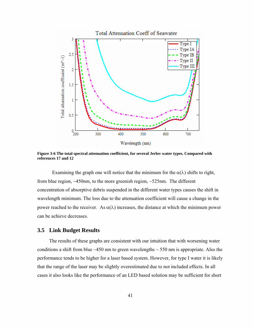
41

Figure 3-6 The total spectral attenuation coefficient, for several Jerlov water types. Compared with references 17 and 12

Examining the graph one will notice that the minimum for the α(λ) shifts to right,

from blue region, ~450nm, to the more greenish region, ~525nm. The different

concentration of absorptive debris suspended in the different water types causes the shift in

wavelength minimum. The loss due to the attenuation coefficient will cause a change in the

power reached to the receiver. As α(λ) increases, the distance at which the minimum power

can be achieve decreases.

3.5 Link Budget Results

The results of these graphs are consistent with our intuition that with worsening water

conditions a shift from blue ~450 nm to green wavelengths ~ 550 nm is appropriate. Also the

performance tends to be higher for a laser based system. However, for type I water it is likely

that the range of the laser may be slightly overestimated due to not included effects. In all

cases it also looks like the performance of an LED based solution may be sufficient for short

42

ranges. Other issues such as the field of view and dynamic range of the receiver will be

important.

The following graphs illustrate this by considering several different water types with

different light sources. It was assumed that a detector capable of detecting signals at the -50

dB level is available; using this one can estimate the expected range for different

wavelengths.

Figure 3-7 1 W LED, in Type II water with particulate, CDOM, chlorophyll, and scattering.

Figure 3-8 10 W Laser, in Type I water with particulate, CDOM, chlorophyll, and scattering.

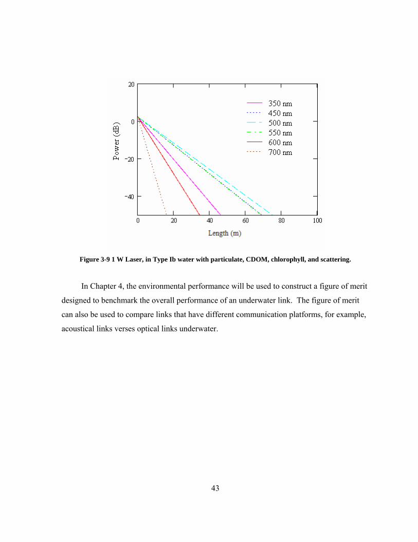
43

Figure 3-9 1 W Laser, in Type Ib water with particulate, CDOM, chlorophyll, and scattering.

In Chapter 4, the environmental performance will be used to construct a figure of merit

designed to benchmark the overall performance of an underwater link. The figure of merit

can also be used to compare links that have different communication platforms, for example,

acoustical links verses optical links underwater.

44

3.6 References

1 J. C. Palais, Fiber Optic Communications, 4th Edition, Prentice Hall, New Jersey, pp 308-316, 1998 2 B. E.A. Saleh, and M.C. Teich, Fundamentals of Photonics, John Wiley & Sons, Inc, New York, 1991 3 S. G. Lambert, W. L. Casey, Laser Communications in Space, Artech House Publishers, Boston, 1995 4 J. Ricklin, A. Mujumdar, SC656 Fundamentals of Free-space Laser communications, SPIE Education Sevices Short Course Notes, Optical Science and Technology, the SPIE 49th Annual Meeting ,2-6 August 2004 Denver CO 5 W.B. Miller, J.C. Ricklin, L.C. Andrews, “Log-Amplitude Variance And Wave Structure-Function - A New Perspective For Gaussian Beams”, J.O.S.A A, 10,661 (1993) 6 F.M. Davidson, S. Bucaille, G.C. Gilbreath, et al. “Measurements of intensity scintillations and probability density functions of retroreflected broadband 980-nm laser light in atmospheric turbulence”, Optical Engineering 43, 2689 (2004) 7 S. Bloom, E. Korevaar, J. Schuster, H. Willerbrand, Understanding the performance of free-space optics.” Journal of Optical Networking, Vol. 2, No. 6, June 2003 8 Milica Stojanovic, Underwater Acoustic Communication, Wiley Encyclopedia of Electrical and Electronics Engineering, Northeastern University Boston, Dept of Electrical and Computer Engineering 9 J. R. Apel, Principles of Ocean Physic, International Geophysics Series, Vol. 38, Academic Press, pg 509-584, 1987 10 H. Arst, Optical Properties and Remote Sensing of Multicomponental Water Bodies, Praxis Publishing, Chichester, UK, pg 8-28, (2003) 11 V.I. Haltrin, Chlorophyll-based model of seawater optical properties, Appl. Opt.,38, No.33, Nov 1999 12 E. Y.S. Young, A.M. Bullock, “Underwater-airborne laser communication system: Characterization of the channel”, Free-Space Laser Communication Technologies XV, G. Stephen Mecherle, Editor, Proceedings of SPIE Vol. 4975 (2003) 13 Excerpted from: Ocean Optics Protocols for Satellite Ocean Color Sensor Validation, Chapter 1 Sections 2 & 3, Rev 4, Volume IV

45

14 C.S. Yentsch, “The Influence of Phytoplankton Pigments on the Color of Sea Water”, Deep-Sea Res., 7, 1, 1960. 15 D.A. Hansell, C.A. Carlson, Biogeochemistry of Marine Dissolved Organic Mater, Academic Press, New York, pg 509-534, (2002) 16 A. Morel, L. Prieur, “Analysis of variations in ocean color,” Limnol, Oceanogr. 22, 709-722, 1977 17 J. Dera, Marine Physics, Elsevier Oceanography Series, Polish Scientific Publishers, New York, pg 220, (1992)

46

Chapter 4 Figure of Merits for Underwater Platform

At first, the figure of merit for comparing communications systems would appear to

be energy per bit and bit-rate length product. One can either consider the attempted

throughput of data or the good throughput of data, or the Bit Error Rate as inputs. It is

simplest to assume the goodput of data through the system, considered as the product of

bitrate and range. The amount of additional encoding to ensure the goodput of data can be

factored in after the initial computation. In many scenarios, for example the transmission of

real-time video, dropping of data bits is not crucial.

However practical underwater communication systems are constrained in size,

weight, and power. There are also additional operational constraints such as minimum speeds

at which the platform can maintain neutral buoyancy and heading especially in the presence

of a current. This can be an important issue when pointing stability between the transmitter

and receiver is required. The problem with this approach is that decisions have to be made

about the relative weighting of different factors. This has been a problem for example in

considering how to compare power systems for underwater vehicles. One can construct a

system for example that has a very high power density which may seem good, but may end

up not being able to reach the desired speed thus defeating the purpose.

To date the use of FOMs for AUV’s for communications has primarily just focused

on the power of the transmitter, the loss of the medium, and the sensitivity of the receiver.

The emphasis has been on achieving more effective gain through signal processing. This

allows one to establish energy per bit value if performed realistically.

First by performing a survey of modern acoustic systems described in the literature,

one can plot the bit rate in kbps verses the range of the system in Figure 4-1. One finds that

there is a relatively constant drop of 20 dB in kbps per decade of range in meters. On a log-

log scale this plots as a straight line roughly demarking the limits of present acoustic systems.

This is a reflection of the 20db/decade drop in SNR that is typical in acoustic systems. As a

point of comparison, the bit rate is compared to a step index multimode optical fiber

operating with light sources at 0.85 um. This represents a very low end, inexpensive photonic

system.

47

The second line of demarcation that is drawn consists of a horizontal line that is set

by the physical limitation of transducers to respond at high frequencies. A very optimistic

value of ~20 MHz was chosen, in the literature, the highest value observed was about 1 MHz

bandwidth.

In Figure 4-1, using the Mclean beam dispersion model and Mobley water data, the

limits for a laser based system in three different water types due to dispersion were computed

and plotted. The upper frequency chose for the laser operation of 10 GHz, which is

somewhat unrealistic, but would be achievable with more sophisticated blue laser designs.

The calculated attenuation was used to set the point where the system becomes power

limited. This coincidentally was close to the distance where the multipath dispersion was

computed. There were two underwater optical communication systems where specifications

were available to be placed on the chart. The first, an LED based system by Ambralux at 10

Mbps and 40 meters fit very well with the calculations. The second system plotted is suspect

and is marked with a question mark. The data was obtained from the company’s website1,

and stated a range of 2 to 3 km for very pure Norwegian seawater, and used a proprietary

receiver of special design. The company was contacted, but was unresponsive in releasing

any details of the system.

48

Figure 4-1 Small blue squares represent Acoustic systems operating in Deep water, Green Triangles represent acoustic systems operating in shallow water2. The red line represents a laser based system, operating in clear ocean water (CLW) environment. The attenuated range is approximately 300 meters. Similar plots are also constructed for Turbid Harbor Water(THW), and Coastal Ocean Water (COW) with correspondingly shorter ranges. The light green region represents area where acoustic systems could be expected to be successful. The light blue region represents where the Optical communications can be expected to compete. For example the red circle at 10 Mbps, with a range of 40 m is an LED based system that has been successfully tested. Note that above 10 Mbps, for distances below 100 meters, it appears that optical systems can be expected to out perform acoustic systems, on the basis of just having a faster bit rate. With current generation lasers, and detectors ~ 100 Mbps, could realistically anticipated for the 10-30 meter range in a variety of water conditions.

4.1 System Level Figure of Merit

The natural way at the system level to divide the figure of merit is to consider the

relative merits of the Transmitter, the Environment, and the Receiver, independently.

RxtEnvironmenTxSystem FOMFOMFOMFOM ⋅⋅=

Writing the FOM in this manner allows one make a calculation for asymmetric platforms for

example a sub and UUV, and include the effects of size and weight of the transmitter and

receiver. Furthermore with a little work, the relative degradation of environmental effects can

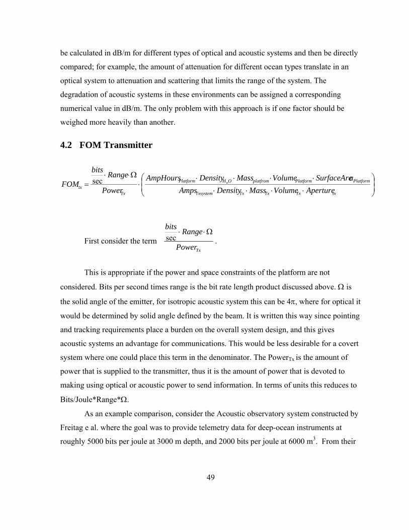
49

be calculated in dB/m for different types of optical and acoustic systems and then be directly

compared; for example, the amount of attenuation for different ocean types translate in an

optical system to attenuation and scattering that limits the range of the system. The

degradation of acoustic systems in these environments can be assigned a corresponding

numerical value in dB/m. The only problem with this approach is if one factor should be

weighed more heavily than another.

4.2 FOM Transmitter

⎟⎟⎠

⎞⎜⎜⎝

⎛

⋅⋅⋅⋅

⋅⋅⋅⋅⋅

Ω⋅⋅=

txTxTxTxTxsystem

PlatformPlatformplatfromOHPlatform

Txtx ApertureVolumeMassDensityAmps

aSurfaceAreVolumeMassDensityAmpHoursPower

Rangebits

FOM wsec

First consider the term TxPower

RangebitsΩ⋅⋅

sec .

This is appropriate if the power and space constraints of the platform are not

considered. Bits per second times range is the bit rate length product discussed above. Ω is

the solid angle of the emitter, for isotropic acoustic system this can be 4π, where for optical it

would be determined by solid angle defined by the beam. It is written this way since pointing

and tracking requirements place a burden on the overall system design, and this gives

acoustic systems an advantage for communications. This would be less desirable for a covert

system where one could place this term in the denominator. The PowerTx is the amount of

power that is supplied to the transmitter, thus it is the amount of power that is devoted to

making using optical or acoustic power to send information. In terms of units this reduces to

Bits/Joule*Range*Ω.

As an example comparison, consider the Acoustic observatory system constructed by

Freitag e al. where the goal was to provide telemetry data for deep-ocean instruments at

roughly 5000 bits per joule at 3000 m depth, and 2000 bits per joule at 6000 m3. From their

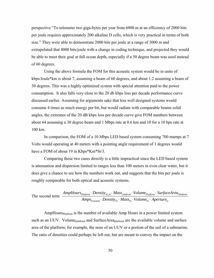
50

perspective “To telemeter two giga-bytes per year from 6000 m at an efficiency of 2000 bits

per joule requires approximately 200 alkaline D cells, which is very practical in terms of both

size.” They were able to demonstrate 2000 bits per joule at a range of 3000 m and

extrapolated that 4000 bits/joule with a change in coding technique, and projected they would

be able to meet their goal at full ocean depth, especially if a 30 degree beam was used instead

of 60 degrees.

Using the above formula the FOM for this acoustic system would be in units of

kbps/Joule*km is about 7, assuming a beam of 60 degrees, and about 1.2 assuming a beam of

30 degrees. This was a highly optimized system with special attention paid to the power

consumption. It also falls very close to the 20 db kbps loss per decade performance curve

discussed earlier. Assuming for arguments sake that less well designed systems would

consume 4 times as much energy per bit, but would radiate with comparable beams solid

angles, the extremes of the 20 dB kbps loss per decade curve give FOM numbers between

about 64 assuming a 30 degree beam and 1 Mbps rate at 0.6 km and 10 for a 10 bps rate at

100 km.

In comparison, the FOM of a 10 Mbps LED based system consuming 700 mamps at 7

Volts would operating at 40 meters with a pointing angle requirement of 1 degrees would

have a FOM of about 19 in Kbps*Km*Sr/J.

Comparing these two cases directly is a little impractical since the LED based system

is attenuation and dispersion limited to ranges less than 100 meters in even clear water, but it

does give a chance to see how the numbers work out, and suggests that the bits per joule is

roughly comparable for both optical and acoustic systems.

The second term txTxTxTxTxsystem

PlatformPlatformplatfromOHPlatform

ApertureVolumeMassDensityAmpsaSurfaceAreVolumeMassDensityAmpHours

w

⋅⋅⋅⋅

⋅⋅⋅⋅

AmpHoursPlatform is the number of available Amp Hours in a power limited system

such as an UUV. Volumeplatform and SurfaceAreaplatform are the available volume and surface

area of the platform; for example, the nose of an UUV or a portion of the sail of a submarine.

The ratio of densities could perhaps be left out, but are meant to convey the impact on the

51

neutral buoyancy of the system. AmpsTxsystem is the total electrical current in amps, including

computational power for signal processing. The units for the portion of the equations in

brackets is hours, and give a product of the operating time available times a unitless number,

expressing the impact of weight and size of the system on the overall platform.

4.3 FOM Environment

BackgroundSolaretcscatteringabsorptionWavelengthfFOMEnviron _),,( += K

This term expressed in mdB is independent of the physical characteristics of the

transmitter and receiver platforms, but does consider their relative physical positions in the

environment and the impact of water type and time of day (solar background). It may be

further modified to include the relative orientation of the receiver with respect to the sun.

This value is calculated using the link budget described above, and penalizes the system by

requiring additional margin to overcome the additional solar interference.

For the optical systems the absorption and scattering model gives the magnitude of

the function f for attenuation limited systems. The effects of solar background are dependent

on the geometry, but are basically the reduction in SNR due to shot noise on the receiver.

For acoustic systems the function f is the loss due to the channel is computed by

considering reductions in the SNR ratio due to the ambient noise level, the self noise of the

platform, the loss in SNR due to Doppler effects due to velocity of the platform, geometric

loss, and the other environmental effects.

52

4.4 FOM Receiver

The receiver FOM is similar to the transmitter FOM, instead of considering the solid

angle of the emitted beam, the field of view (FOV) of the Aperture is considered.

⎟⎟⎠

⎞⎜⎜⎝

⎛

⋅⋅⋅⋅

⋅⋅⋅⋅⋅

⋅=

RxRxRxRxRxsystem

PlatformPlatformplatfromOHPlatform

reciever

FOVRx ApertureVolumeMassDensityAmps

aSurfaceAreVolumeMassDensityAmpHoursPower

AperturebitrateFOM w

A certain amount of optical energy per bit is required to have a detectible signal and

is equivalent to the bit-rate divided by the receiver power. A larger acceptance angle for the

receiver is desirable, and conveys the pointing requirement that optical systems have. For

acoustic systems the FOV concept would be replaced by an effective directivity of the

hydrophone if the hydrophone is not directional.

In Chapter 5, experimental circuits and data will be presented related to constructed

prototype LED communication links that could be used in several undersea applications.

These experiments range from examining high powered LEDs, building an FM modulated 2-

way voice communication link, and the construction of a full duplex 10 Mbps optical link.

4.5 References

1 The claim of 2 to 3 km was found on the world wide web at http://www.laseroptronix.se/subsea/modem.html 2 Data complied from, Ian F. Akyildiz, Dario Pompili, Tommaso Melodia, Underwater acoustic sensor networks: research challenges, To be published in Ad Hoc Networks (2005), and Milica Stojanovic “Underwater Acoustic Communication” article for Wiley Encyclopedia of Electrical and Electronics Engineering. 3 Lee Freitag, Mark Johnson and Daniel Frye, “High-Rate Acoustic Communications for Ocean Observatories-Performance Testing Over a 3000 m Vertical Path” OCEANS 2000 MTS/IEEE Conference and Exhibition Volume 2, 1443 (2000)

53

Chapter 5 Experimental Data and Circuitry

5.1 High Powered LEDS

Recently, high powered LEDs have been commercialized for applications requiring

high efficiency including automobile head lights, brake lighting, and indoor lamp lighting.

As a possible future application the possibility of using high powered LEDs for underwater

communications were explored where the desired wavelengths of operation are between

450nm and 550nm. As described in chapter 3 these wavelength have the least attenuation in

ocean water. For optical communication purposes the following aspects should be

considered:

• Optical wavelength

• Optical output power

• Reliability

• Beam parameters.

LumiLEDs are presently the industry leader in high powered LEDs. They have focused on

efficiently extracting light from the LEDs and packaging the LEDs so that heat can

efficiently be removed. They have three LED wavelengths that could be considered for

underwater applications, Blue, Cyan, and Green. The spectrum for each color LED can be

seen in the graph below.

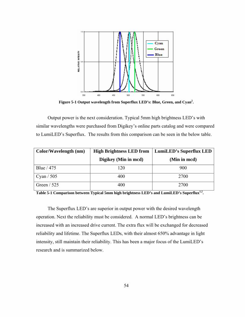
54

Figure 5-1 Output wavelength from Superflux LED’s: Blue, Green, and Cyan2.

Output power is the next consideration. Typical 5mm high brightness LED’s with

similar wavelengths were purchased from Digikey’s online parts catalog and were compared

to LumiLED’s Superflux. The results from this comparison can be seen in the below table.

Color/Wavelength (nm) High Brightness LED from

Digikey (Min in mcd)

LumiLED’s Superflux LED

(Min in mcd)

Blue / 475 120 900

Cyan / 505 400 2700

Green / 525 400 2700 Table 5-1 Comparison between Typical 5mm high brightness LED’s and LumiLED’s Superflux1,2.

The Superflux LED’s are superior in output power with the desired wavelength

operation. Next the reliability must be considered. A normal LED’s brightness can be

increased with an increased drive current. The extra flux will be exchanged for decreased

reliability and lifetime. The Superflux LEDs, with their almost 650% advantage in light

intensity, still maintain their reliability. This has been a major focus of the LumiLED’s

research and is summarized below.

55

Stress Condition Failure Rate

Temp = 55 C, I = 70 mA <0.027

Temp = 85 C, I = 45 mA <0.30

Temp = -40 C, I = 70 mA <0.06 Table 5-2 Reliability testing of Lumiled’s Superflux LED’s from Ref 2

In many LED applications the characteristics of the output beam are not that

important; however in an optical communications system the ability to collimate a beam is

very important. In a conventional packaged LED the semiconductor material is seated in a

reflective cup with two terminal leads which is all incased in a transparent epoxy. One of the

leads is located at the base with the other wirebonded to the top of the die.

Figure 5-2 Conventional packaged LED, Right) LumiLED’s package Superflux LED

In the case of GaN LEDs on sapphire substrates there are two top contacts since the

sapphire is insulating. The combination of the reflective cup, plastic epoxy, and lead

overhang in a conventional LED, leads to a distorted light image. This causes and increases

the difficulty of forming a collimated beam. The Superflux LEDs have a similar setup as a

typical LED, but LumiLED has optimized the design such that the image is not distorted, in

addition to taking special care forming a good lens with the epoxy. When focused, the

illuminated LED die can be seen very clearly with minimal distortion. Even the overhang

has been minimized.

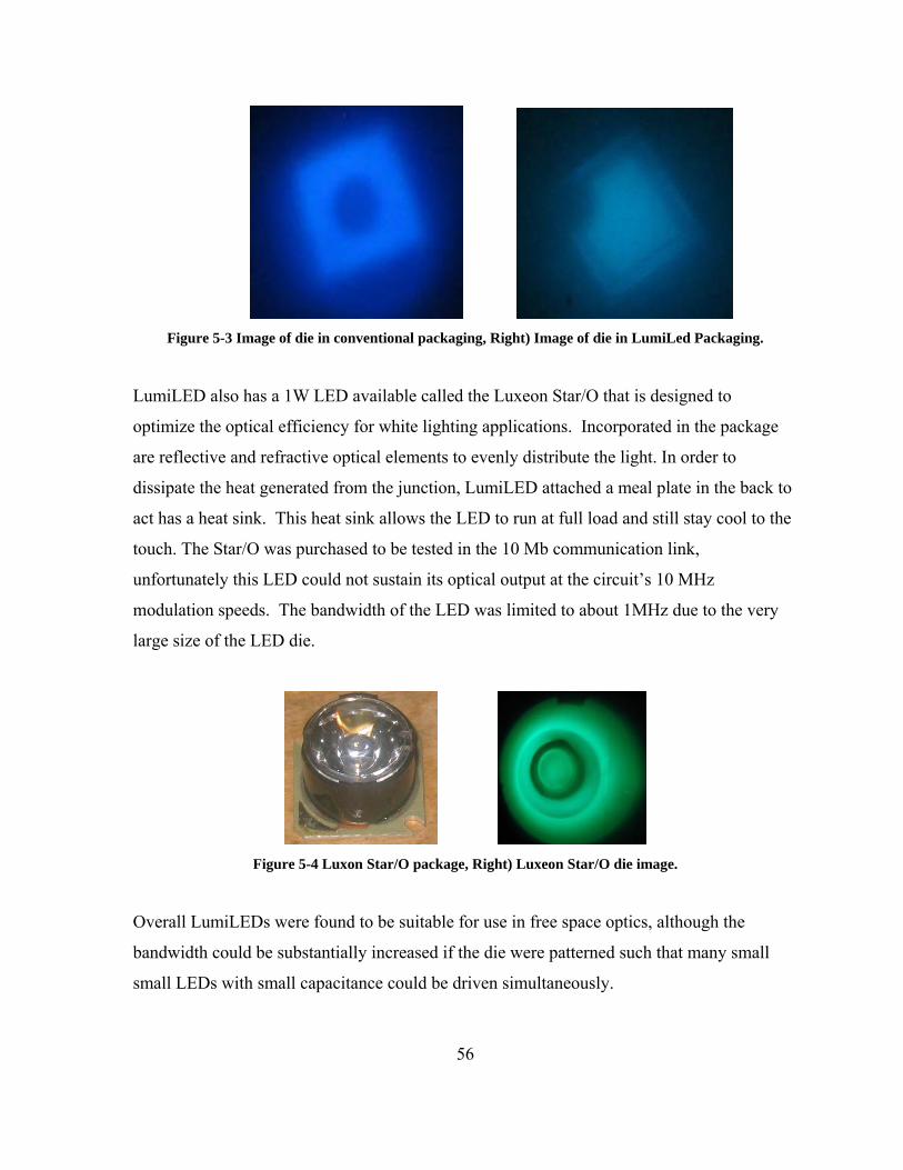
56

Figure 5-3 Image of die in conventional packaging, Right) Image of die in LumiLed Packaging.

LumiLED also has a 1W LED available called the Luxeon Star/O that is designed to

optimize the optical efficiency for white lighting applications. Incorporated in the package

are reflective and refractive optical elements to evenly distribute the light. In order to

dissipate the heat generated from the junction, LumiLED attached a meal plate in the back to

act has a heat sink. This heat sink allows the LED to run at full load and still stay cool to the

touch. The Star/O was purchased to be tested in the 10 Mb communication link,

unfortunately this LED could not sustain its optical output at the circuit’s 10 MHz

modulation speeds. The bandwidth of the LED was limited to about 1MHz due to the very

large size of the LED die.

Figure 5-4 Luxon Star/O package, Right) Luxeon Star/O die image.

Overall LumiLEDs were found to be suitable for use in free space optics, although the

bandwidth could be substantially increased if the die were patterned such that many small

small LEDs with small capacitance could be driven simultaneously.

57

5.2 High Powered Pulser Circuit using ZTX415 Avalanche Transistors

The purpose of this experiment was to understand what happens to the properties of an

LED when pulsed with high current for short periods of time. The advantages of high current

nanosecond pulsed operation is that:

• The higher current pulses will the increased amount of light to be produced form the

LED

• Allow for better heat dissipation, since the LED is “off” the majority of the time

T. Araki et al.3, constructed a pulser circuit that was used to produce ultraviolet nanosecond

light pulses from a blue light emitting diode. Under conventional operation of 20mA, the

InGaN/AlGaN blue LED would output 450nm, but operating above 50mA an increasing

amount of 380nm light was produced.

R.J. Baker et al.4, used normal 2N3904 transistors to produce high voltage pulser. A

2000V pulse generator with a rise-time of 1ns and with less than 100 ps of jitter was

produced as a result of that research. For the purposes of our research, the circuit by T. Araki

et al.3 was constructed due to its simplicity and narrow output pulses. The circuit was used to

pulse a Superflux blue LED manufactured by LumiLED.

Figure 5-5 Circuit diagram of 4ns light pulse generator, Right) Circuit board of the pulse generator

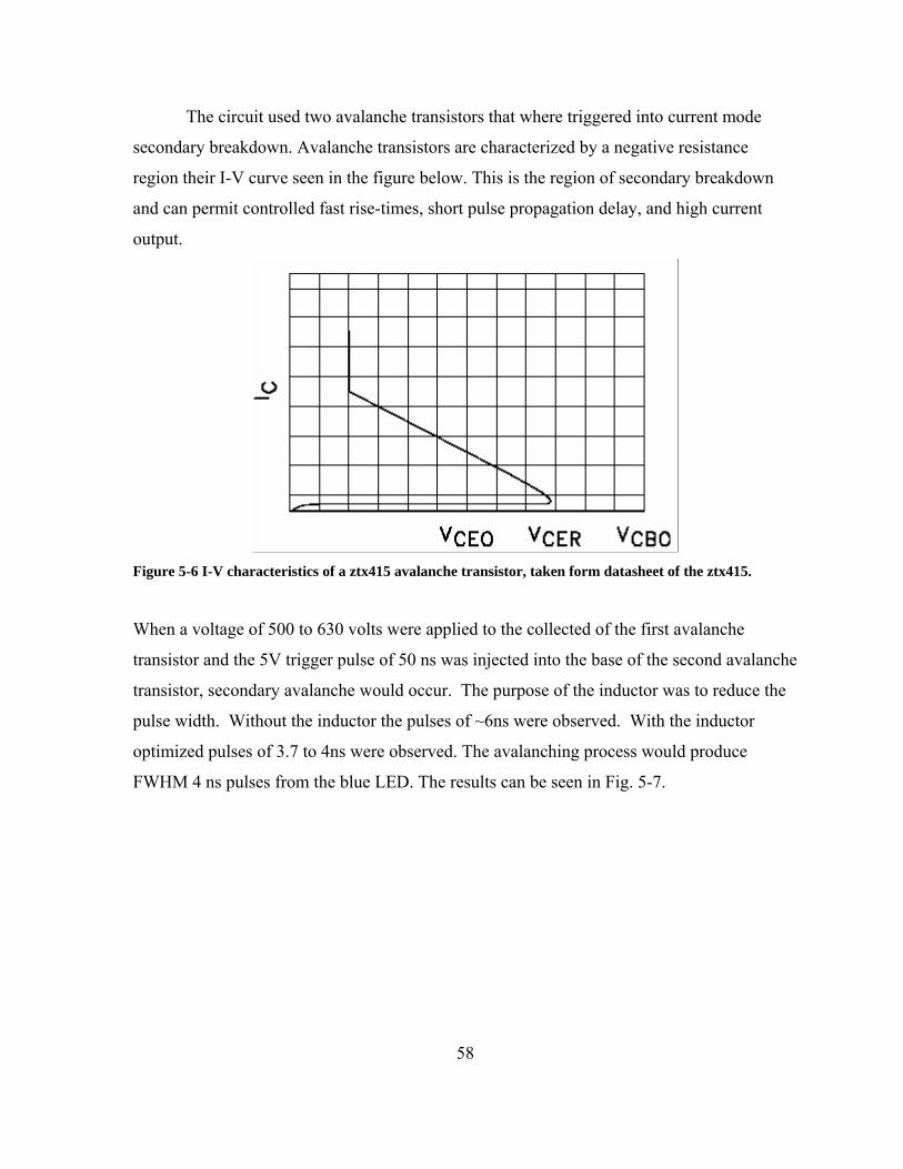
58

The circuit used two avalanche transistors that where triggered into current mode

secondary breakdown. Avalanche transistors are characterized by a negative resistance

region their I-V curve seen in the figure below. This is the region of secondary breakdown

and can permit controlled fast rise-times, short pulse propagation delay, and high current

output.

Figure 5-6 I-V characteristics of a ztx415 avalanche transistor, taken form datasheet of the ztx415.

When a voltage of 500 to 630 volts were applied to the collected of the first avalanche

transistor and the 5V trigger pulse of 50 ns was injected into the base of the second avalanche

transistor, secondary avalanche would occur. The purpose of the inductor was to reduce the

pulse width. Without the inductor the pulses of ~6ns were observed. With the inductor

optimized pulses of 3.7 to 4ns were observed. The avalanching process would produce

FWHM 4 ns pulses from the blue LED. The results can be seen in Fig. 5-7.

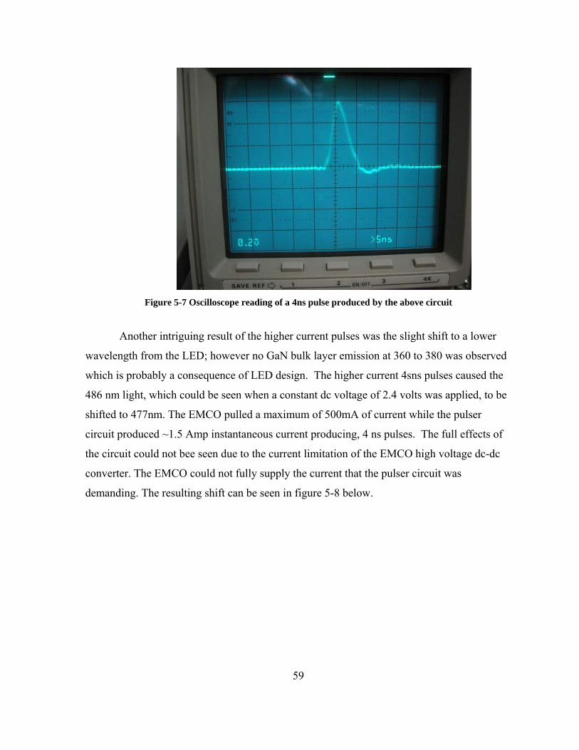
59

Figure 5-7 Oscilloscope reading of a 4ns pulse produced by the above circuit

Another intriguing result of the higher current pulses was the slight shift to a lower

wavelength from the LED; however no GaN bulk layer emission at 360 to 380 was observed

which is probably a consequence of LED design. The higher current 4sns pulses caused the

486 nm light, which could be seen when a constant dc voltage of 2.4 volts was applied, to be

shifted to 477nm. The EMCO pulled a maximum of 500mA of current while the pulser

circuit produced ~1.5 Amp instantaneous current producing, 4 ns pulses. The full effects of

the circuit could not bee seen due to the current limitation of the EMCO high voltage dc-dc

converter. The EMCO could not fully supply the current that the pulser circuit was

demanding. The resulting shift can be seen in figure 5-8 below.

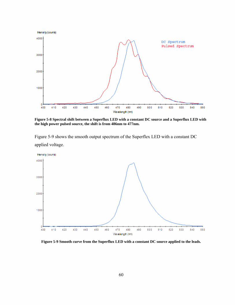
60

Figure 5-8 Spectral shift between a Superflux LED with a constant DC source and a Superflux LED with the high power pulsed source, the shift is from 486nm to 477nm.

Figure 5-9 shows the smooth output spectrum of the Superflex LED with a constant DC

applied voltage.

Figure 5-9 Smooth curve from the Superflux LED with a constant DC source applied to the leads.

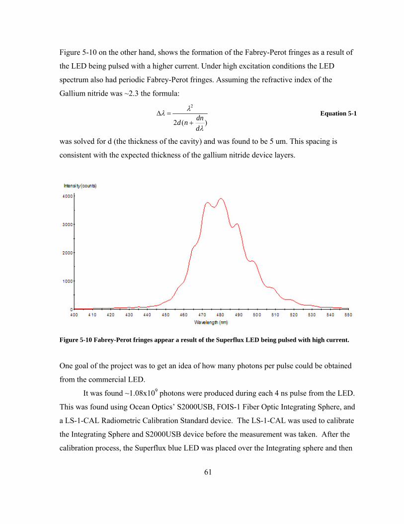
61

Figure 5-10 on the other hand, shows the formation of the Fabrey-Perot fringes as a result of

the LED being pulsed with a higher current. Under high excitation conditions the LED

spectrum also had periodic Fabrey-Perot fringes. Assuming the refractive index of the

Gallium nitride was ~2.3 the formula:

)(2

2

λ

λλ

ddnnd +

=∆ Equation 5-1

was solved for d (the thickness of the cavity) and was found to be 5 um. This spacing is

consistent with the expected thickness of the gallium nitride device layers.

Figure 5-10 Fabrey-Perot fringes appear a result of the Superflux LED being pulsed with high current.

One goal of the project was to get an idea of how many photons per pulse could be obtained

from the commercial LED.

It was found ~1.08x109 photons were produced during each 4 ns pulse from the LED.

This was found using Ocean Optics’ S2000USB, FOIS-1 Fiber Optic Integrating Sphere, and

a LS-1-CAL Radiometric Calibration Standard device. The LS-1-CAL was used to calibrate

the Integrating Sphere and S2000USB device before the measurement was taken. After the

calibration process, the Superflux blue LED was placed over the Integrating sphere and then

62

shielded from outside light sources. With the 4 ns pulser running at a repletion rate of 1

MHz, the optical power produced was 45 uW in a 100ms interval.

Using the formula:

λhcPN t

photon = Equation 5-2

Where Nphoton is the total number of photons, Pt is the total optical power collected by the

Integrating Sphere, h=6.626x10-34 is Plank’s constant, c=3x108 is the speed of light in a

vacuum, and λ is the wavelength of operation. The output wavelength of the light source is

477 nm. In 100 ms, a 1 MHz pulsed signal will pulse a total of 100,000 times. Divide

Equation 5-2 by 100,000 and the photon count will be as stated above. This result is

consistent with about ~109 photons per pulse that was observed in R.V. Vasil’ev et al.5.

Two main problems were found when working with the pulser circuit. When the

modulation speed was too high the ¼ Watt 60 k-ohm resistor would begin to overheat and

eventually burn out. A 3 W was replaced to prevent this and to keep from having to

constantly change the resistor after each experimental run. Even the 3W resistor would get

hot to the touch and the circuit would have to be turned off and cooled. To supply the 600+

volts needed for the avalanche transistors an EMCO high voltage dc-dc converter was used

with a 1000V maximum output and 15mA current rating. Even though the voltage was

correct, the maximum amount of current was limited through the device. The pulsed current

limit was not known by the manufacture, but was much higher than the rated current of 15

mA. However, the power supply still limited the amount of current produced by the

avalanching process. When the current pulses were limited this could be seen by the voltage

of the power supply dropping. In general the avalanche transistor could probably have

supplied more current per pulse thus the full effects of the avalanching the transistors was not

seen.

With the proper equipment this circuit could be very usefully in producing very short,

high powered optical pulses from convention LEDs as an alternative to expensive lasers.

However, the main expense of the approach is the high voltage supply.

63

5.3 FM Optical Wireless System

The next experiment demonstrated the use of LEDs in a simple communication link

using human voice. FM modulation was chosen over AM modulation since it was viewed as

being more resistant to fading and variations in the signal amplitude. There were two

versions of the Circuit built. The first version used the 4ns pulser circuit, seen below

Figure 5-11 First generation FM wireless circuit with high power 4 ns pulser as LED driver

This worked fine even though the duty cycle of the pulses was extremely short (4ns at

100kHz). This was accomplished by using a Schmitt Trigger to recognize when a pulse was

received and convert the signal into a 50% duty cycle square-wave. To produce a system

with lower overall power requirements as second generation was also constructed that uses a

logic chip as the LED driver. In this circuit the Schmitt Trigger was not necessary since the

duty cycle of ~50% was created by the LED driver. The populated board of the second

generation chip is shown in Figure 5-12 below.

64

Figure 5-12 Circuit Diagram of FM 2-way voice LED link

The output of the circuit was not a 4 ns pulse but it had a nice 3.5 volt square-wave output

with a 50% duty cycle. The NE564 phase-locked loop had an easier time locking on to a 50%

which deleted some of the pulse cleaning circuitry on the front end of the receiver. A block

diagram of the second generation board can be seen below.

65

Figure 5-13 Circuit block diagram of FM optical wireless system

Transmitter

• Microphone

The microphone circuit consisted of the microphone and resistors and capacitor

network. The resistors that are chosen are crucial for its proper functionality. If the value is

too large, the audio amplifier will become saturated and clip the incoming audio signal. If

the value is too small, the microphone will not be sensitive enough to use at a reasonable

distance.

• Band-pass Filter & Audio Amplifier

The voice is then sent through a band-pass filter. The band-pass filter is 1st order

filter using passive components set for the voice frequency (VF). Even though the human

voice is capable of sounds between 100Hz to 10 kHz, capacitors and resistors were chosen to

pass signal from 300Hz to 5kHz since these are the main useful frequencies. Filtering the

66

signal also reduces background and white noise. The filtered signal was then amplified with

a LM386 audio amplifier with 10X gain. This gave a 1 to 2 volt signals for reasonable sound

pressure levels on the microphone.

• Voltage Controlled Oscillator

A Voltage Controlled Oscillator is an oscillator that changes its frequency according

to a control voltage feed to its control input. An ICL8038 precision waveform

generator/voltage controlled oscillator was used to generate the frequency modulated output

to the LED pulser circuit. It was difficult to find a voltage to frequency converter in the 100

kHz range and this synthesizer chip provided a relatively simple solution. An additional

advantage of this chip is that it has small temperature coefficients resulting is a stable

frequency.

The output of the oscillator is a 50% duty cycle square-wave set to a center frequency of

100 kHz. The frequency was set by two external resistors and one external capacitor. Load

impedances have to be taken into account due to the sensitivity of the IC. If the load

resistance was to change due to temperature, pressure, or if circuit sees a voltage drop due to

battery drain, then the VCO has the potential to change center frequencies. This was

observed experimentally when the load of the LED pulser circuit changed very slightly,

roughly 2-4 ohms due to the battery supply being drained, one could see a swing in

frequencey of plus and minus 10-20 kHz.

It was observed that when the external frequency setting resistor and capacitor shifted

due temperature fluctuation, the center frequency would shift. The receiving circuit would

have a hard time demodulating the shifted signal, thus causing signal degradation. The use

of a crystal oscillator instead of the set resistor and capacitor could potential solve this issue.

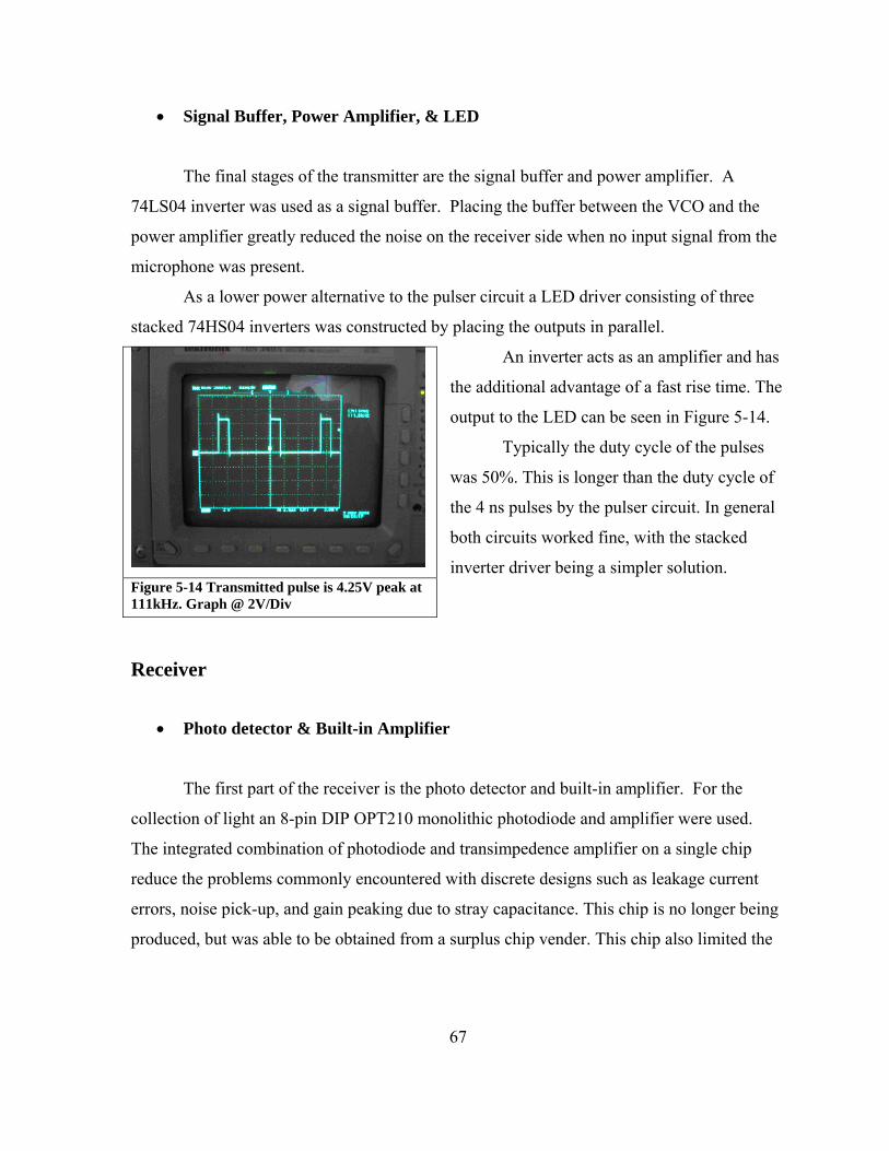
67

• Signal Buffer, Power Amplifier, & LED

The final stages of the transmitter are the signal buffer and power amplifier. A

74LS04 inverter was used as a signal buffer. Placing the buffer between the VCO and the

power amplifier greatly reduced the noise on the receiver side when no input signal from the

microphone was present.

As a lower power alternative to the pulser circuit a LED driver consisting of three

stacked 74HS04 inverters was constructed by placing the outputs in parallel.

An inverter acts as an amplifier and has

the additional advantage of a fast rise time. The

output to the LED can be seen in Figure 5-14.

Typically the duty cycle of the pulses

was 50%. This is longer than the duty cycle of

the 4 ns pulses by the pulser circuit. In general

both circuits worked fine, with the stacked

inverter driver being a simpler solution.

Receiver

• Photo detector & Built-in Amplifier

The first part of the receiver is the photo detector and built-in amplifier. For the

collection of light an 8-pin DIP OPT210 monolithic photodiode and amplifier were used.

The integrated combination of photodiode and transimpedence amplifier on a single chip

reduce the problems commonly encountered with discrete designs such as leakage current

errors, noise pick-up, and gain peaking due to stray capacitance. This chip is no longer being

produced, but was able to be obtained from a surplus chip vender. This chip also limited the

Figure 5-14 Transmitted pulse is 4.25V peak at 111kHz. Graph @ 2V/Div

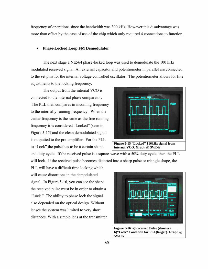
68

frequency of operations since the bandwidth was 300 kHz. However this disadvantage was

more than offset by the ease of use of the chip which only required 4 connections to function.

• Phase-Locked Loop FM Demodulator

The next stage a NE564 phase-locked loop was used to demodulate the 100 kHz

modulated received signal. An external capacitor and potentiometer in parallel are connected

to the set pins for the internal voltage controlled oscillator. The potentiometer allows for fine

adjustments to the locking frequency.

The output from the internal VCO is

connected to the internal phase comparator.

The PLL then compares in incoming frequency

to the internally running frequency. When the

center frequency is the same as the free running

frequency it is considered “Locked” (seen in

Figure 5-15) and the clean demodulated signal

is outputted to the pre-amplifier. For the PLL

to “Lock” the pulse has to be a certain shape

and duty cycle. If the received pulse is a square-wave with a 50% duty cycle, then the PLL

will lock. If the received pulse becomes distorted into a sharp pulse or triangle shape, the

PLL will have a difficult time locking which

will cause distortions in the demodulated

signal. In Figure 5-16, you can see the shape

the received pulse must be in order to obtain a

“Lock.” The ability to phase lock the signal

also depended on the optical design. Without

lenses the system was limited to very short

distances. With a simple lens at the transmitter

Figure 5-15 “Locked” 116kHz signal from internal VCO. Graph @ 5V/Div

Figure 5-16 a)Received Pulse (shorter) b)“Lock” Condition for PLL(larger). Graph @ 5V/Div

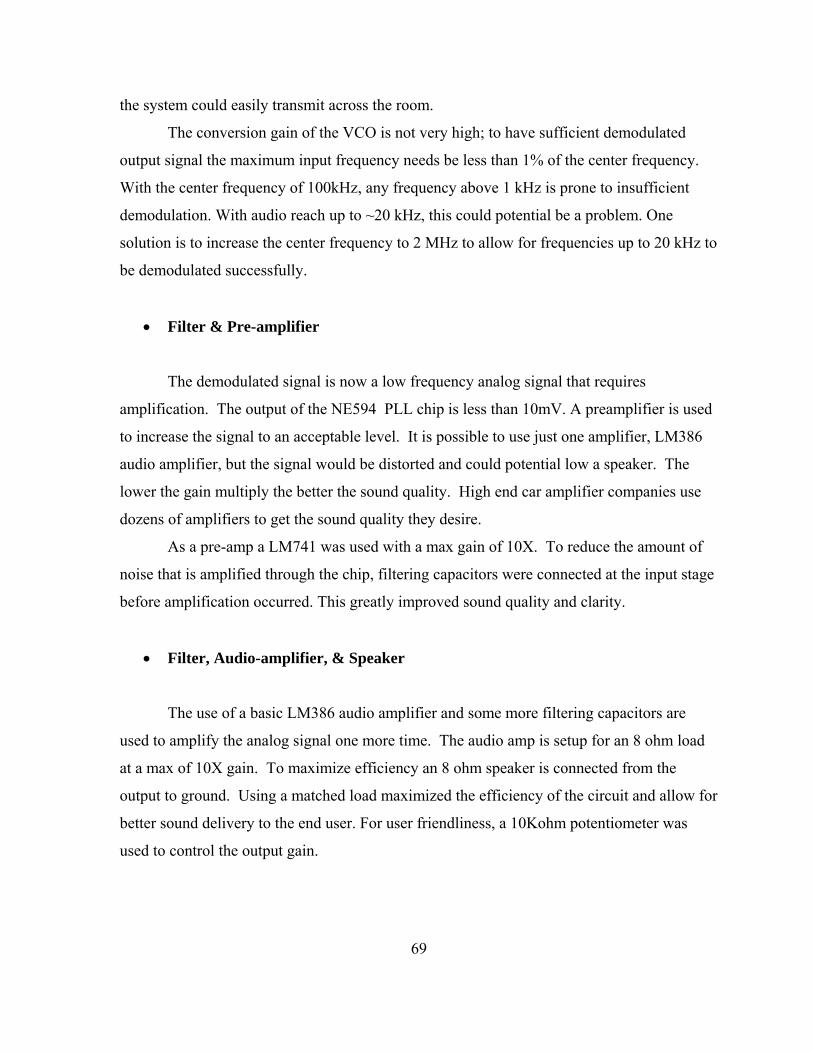
69

the system could easily transmit across the room.

The conversion gain of the VCO is not very high; to have sufficient demodulated

output signal the maximum input frequency needs be less than 1% of the center frequency.

With the center frequency of 100kHz, any frequency above 1 kHz is prone to insufficient

demodulation. With audio reach up to ~20 kHz, this could potential be a problem. One

solution is to increase the center frequency to 2 MHz to allow for frequencies up to 20 kHz to

be demodulated successfully.

• Filter & Pre-amplifier

The demodulated signal is now a low frequency analog signal that requires

amplification. The output of the NE594 PLL chip is less than 10mV. A preamplifier is used

to increase the signal to an acceptable level. It is possible to use just one amplifier, LM386

audio amplifier, but the signal would be distorted and could potential low a speaker. The

lower the gain multiply the better the sound quality. High end car amplifier companies use

dozens of amplifiers to get the sound quality they desire.

As a pre-amp a LM741 was used with a max gain of 10X. To reduce the amount of

noise that is amplified through the chip, filtering capacitors were connected at the input stage

before amplification occurred. This greatly improved sound quality and clarity.

• Filter, Audio-amplifier, & Speaker

The use of a basic LM386 audio amplifier and some more filtering capacitors are

used to amplify the analog signal one more time. The audio amp is setup for an 8 ohm load

at a max of 10X gain. To maximize efficiency an 8 ohm speaker is connected from the

output to ground. Using a matched load maximized the efficiency of the circuit and allow for

better sound delivery to the end user. For user friendliness, a 10Kohm potentiometer was

used to control the output gain.

70

5.4 RONJA, 10Mbps Optical Data Link

The idea of RONJA originated in Czech Republic in 1998, with a prototype model

developed in 2001. The idea was to create a fast but relatively inexpensive way to create a

network over a fairly long distance without using any sort of wiring infrastructure. The

original RONJA cost about $200 to construct and has been implemented in many places in

Eastern Europe; one European university uses the RONJA technology as their primary means

of providing Internet access to their dormitories. References to the RONJA project can be

found at www.twibright.com by Mgr. Mikuláš Patočka, Mgr. Petr Kulhavý, Mgr. Martin

Pergel, Mgr. Karel Kulhavý.

The RONJA (Reasonable Optical Near Joint Access) device is a point-to-point

mechanism that allows two sources to transmit and receive data using a modulated beam of

light. RONJA uses a high intensity LED to modulate light to transfer data up to a distance of

1.4 km at a speed of 10 Mbps. RONJA consists of three modules: a transmitter, a receiver,

and an interface to the source. The goal of the project was to improve this design such that is

would be suitable for underwater communication.

Design

There were two parts to the project. The first part is the mechanical/optical

enclosures that house the lenses and copper boxes containing the receiver and transmitter

circuits. This enclosure had to be waterproof, but accessible if lenses or circuits ever

required maintenance/repair. The second part of the system is the electrical circuits including

the UTP, receiver and transmitter. Below is a breakdown of each part and their operation.

71

Electrical/Circuit

UTP (Universal Twisted Pair)

Figure 5-17 Functional block diagram of the Twisted Pair Interface. Full circuit diagrams in Appendix B

UTP – The UTP (Universal Twisted Pair) is the main interface to the PC. The signal from

the RJ-45 port goes into the RJ-45 Filter. The schematic below shows the pin layout of the

RJ-45 filter. This filter isolates the board from outside noise. The RJ-45 standard calls for

twisted pair wires consisting of a positive and negative wire for the transmit and receive, for

a total of 4 wires. This differential output setup is used to reduce any noise the Ethernet

cable may receive from outside sources. The positive and negative transmit signal are on

pins 9 and 11 of the filter. The respective receiver pins are 14 and 16. This can be seen in

the schematic below. The signal is then passed into the transmitter circuit of the UTP.

72

TX Circuit– The transmitter establishes the handshaking between the idle signal and the data

stream in preparation to be sent to the LED transmission board.

- MC3486 (Quad Differential Line Receiver) – This IC multiplexes the two differential

transmission signals (positive and negative) into one signal.

- 74HC74N (Dual D-Type Flip-Flop w/ Set and Reset) – This IC provides a 1MHz idle

signal for the LED. This signal is for maintaining a defined DC level and to prevent

receiver noise and unwanted signals from being amplified in the limiter on the receiver

board. The system would not work without the 1MHz signal. Packets would be randomly

lost due to received packet echoes from the opposite direction on shorter links, sometimes

even on longer links due to random noise resembling a preamble, and most importantly,

the remaining packet would not be received at all because the corrupted preamble would

be received by the RJ-45 interface.

- 74HC14N (Hex Inverting Schmitt Trigger) and 74HC132N (Quad Schmitt Trigger

NAND Gate) – These ICs work together to decide if the idle signal or data signal should

be passed. If no packet is detected, the idle signal is passed. When a data signal is

detected, the idle signal is dropped. The red indicator LED on the board is flashed to

indicate transmission activity.

73

RX Circuit - This circuit filters out the 1MHz signal, passes the data signal to a de-

multiplexer, passes the (positive and negative) signals to the RJ-45 filter which then passes

them to their respective receive wires on the RJ-45 port.

- 74HC74N (Dual D-Type Flip-Flop w/ Set and Reset) – Produces Ethernet standard

250Hz (NLP or Normal Link Pulse) signal which tells the PC the UTP is an Ethernet

compatible device. Every 4ms this NLP is sent to the PC maintaining the compatibility

status.

- Common Emitter Pair – Pre-amplifier for incoming ~700mVpp to ~4Vpp. This

increases the current and voltage so that incoming pulse train will trigger the input of the

74HC14N.

- 74HC14N (Hex Inverting Schmitt Trigger) and 74HC132N (Quad Schmitt Trigger

NAND Gate) – Rejects the 1MHz idle signal so that it is not passed to the PC. If a data

signal is detected it passes the signal, otherwise the 250Hz NLP is sent to the PC for the

reasons described above. The green indicator LED on the board flashes to indicate

reception activity.

- MC3487 (Quad Differential Line Driver) – This IC de-multiplexes the incoming data

signal into separate differential output (positive and negative) receive signals for the RJ-

45 filter and port.

Transmitter

Figure 5-18 Functional block diagram of the transmitter board, Right) The transmitter circuit. Full circuit diagram in Appendix B.

74

The signal arrives via the coaxial connection. The DC filter removes any DC offset, which

leaves a pure square wave. Before the signal is transmitted, the signal must be current

amplified to push the LED. This is accomplished by an emitter coupled transistor pair

(preamp) and by stacking three 74HC04 ICs. The signal is then ready for transmission via

the cyan LED.

Receiver

Figure 5-19 Functional block diagram of the receiver board, Right) The receiver circuit. Full circuit diagram in Appendix B

The receiver detects the photons via the photo detector. The low current signal triggers a

dual gate transistor (NTE415) which takes the current from the 12V rail and transmits it to

the NE592 video amplifier. The NE592 cleans the incoming rounded signal to a square

wave. Pin 7 of the NE592 is part of a differential output which is used to measure the signal

strength based on the alignment of the optical signal. This is called the received signal

strength indicator (RSSI). Pin 8 of the NE592 is the other part of the differential output and

carries the data stream through a pre-amp/limiter circuit consisting of a pair of common

emitter connected transistors which limits the signal to ~700mVpp. The signal is then sent to

the receiving end of the UTP.

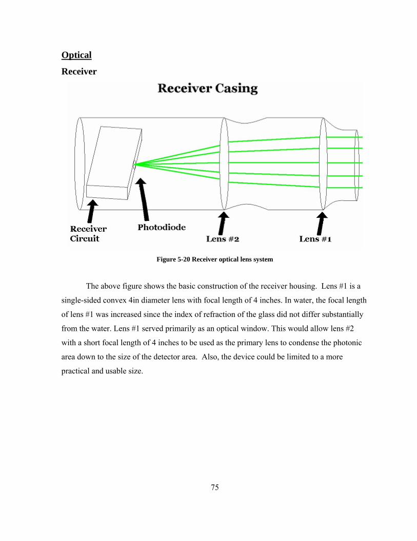
75

Optical

Receiver

Figure 5-20 Receiver optical lens system

The above figure shows the basic construction of the receiver housing. Lens #1 is a

single-sided convex 4in diameter lens with focal length of 4 inches. In water, the focal length

of lens #1 was increased since the index of refraction of the glass did not differ substantially

from the water. Lens #1 served primarily as an optical window. This would allow lens #2

with a short focal length of 4 inches to be used as the primary lens to condense the photonic

area down to the size of the detector area. Also, the device could be limited to a more

practical and usable size.

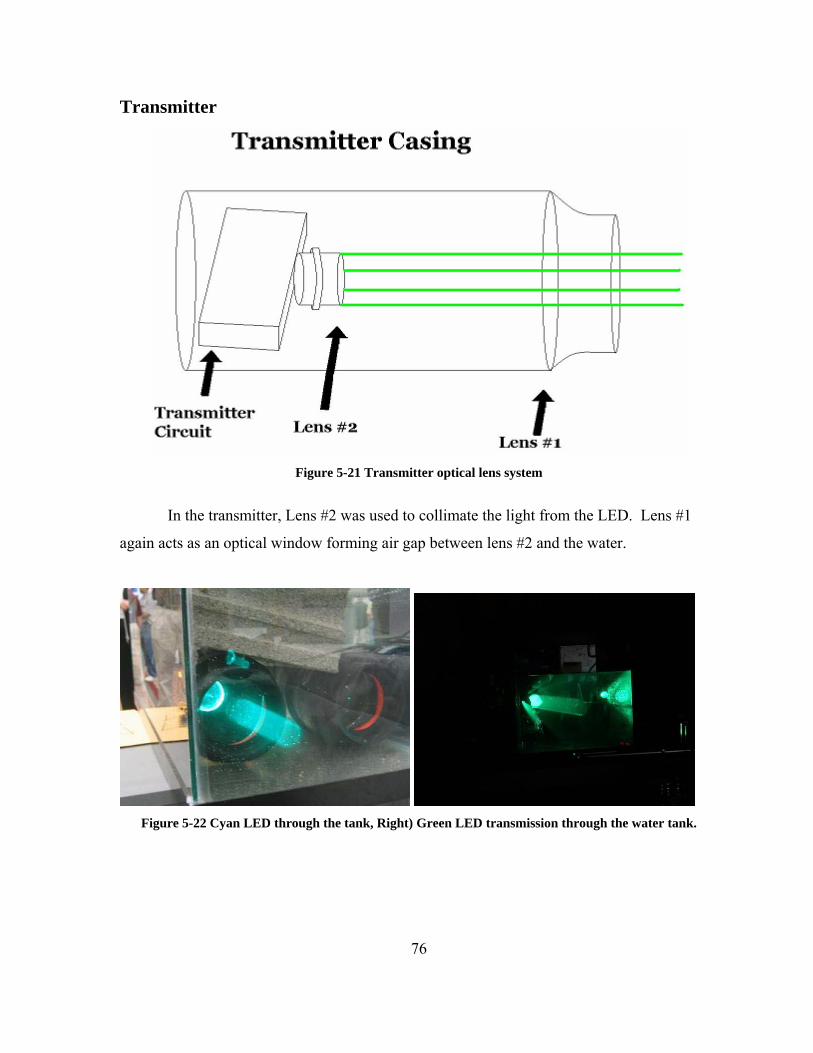
76

Transmitter

Figure 5-21 Transmitter optical lens system

In the transmitter, Lens #2 was used to collimate the light from the LED. Lens #1

again acts as an optical window forming air gap between lens #2 and the water.

Figure 5-22 Cyan LED through the tank, Right) Green LED transmission through the water tank.

77

The result of the above lens networks are a fairly collimated LED beam through the water.

Though the beam is not perfectly collimated, it was able to travel 140 feet and only grow to 2

times the original diameter giving a divergence of 1.19 mrads.

Mechanical

The underwater casing was constructed from 4” ABS tubing purchased from Lowe’s

Home Improvement. Water tight wire connections were used with the addiction of water

proof marine sealant to make the holes for the coax cables to exit/enter the tubes. These

connectors can be seen in Figure 5-23 below.

Figure 5-23 Water proof coaxial cable connector, Right) Water proofed Lens sealing

The tubes from the transmitter and receiver were similar in deign, but the receiver had

an extra 4” lens that the transmitter lacked. The second 4” lens was the primary focusing

lens while the first just acted as an optical window. Since the index of refraction of the water

and lens were so close, the focal length was stretched from 4 inches to almost 4 feet.

The 4 inch lenses were seated in the 4” diameter section of 3” to 4” couplers. The

lenses were then sealed with aquarium sealant and then rubber hosing was used a cushion

between the lens and 3” ABS tube that pressed up against it. When the tubes are submitted to

78

higher water pressures, the pressure would cause the lenses to push in and could eventually

break the seal. So the hosing acted as a cushioned compressor against the 3” ABS tube.

For the receiver, another 3” to 4” coupler was used to seat the second 4” lens the

same was as above. Then a piece of 4” pipe was measured and cut just enough to seat the

coupler flush to the 4” to 4” coupler. A 4” threaded back was used so that the circuit could be

accessed for chip replacement or realignment issues. The transmitter was built the same way

with the absence of the extra 3” to 4” coupler. A picture of the constructed tubes can be seen

below.

Figure 5-24 The two tubes on the left are the receivers and the tubes on the right are the transmitters.

After the casing was complete, the tubes were submerged for 4 hrs to test for water

leaks. The water leak test proved successful in a 20 gallon aquarium. The circuits (in copper

shielded boxes) were then anchored to the tubes at the proper focal points. The tubes with

the circuits were then placed in the water and the link was validated. Below is a 10MHz

waveform after passing through two 20 gallon water tanks spaced 15 feet apart.

79

Figure 5-25 A 10MHz signal after passing through the water tank, Right) Screenshot of RONJA successfully testing at 10Mbps

The 10 Mbps link was also successfully obtained between two computers, but

complications with the receiver circuit caused severe alignment issues. The suspicion is the

dual gate transistor on the front end of the receiver circuit, just after the photodiode, is not

fast enough to switch the Manchester encoded 10 Mbps signal. Some of the bits do not make

a full swing to the negative or positive railing causing corruption of the signal. This will be

research more in future work.

However, when care was taken to properly align the system, its full 10 Mbps

operation was verified with video link established between two computers at distances of

about 40 feet. Continuous ftp transferring of large files between the two computers for 6

hours without significant dropout problems with the network was also observed.

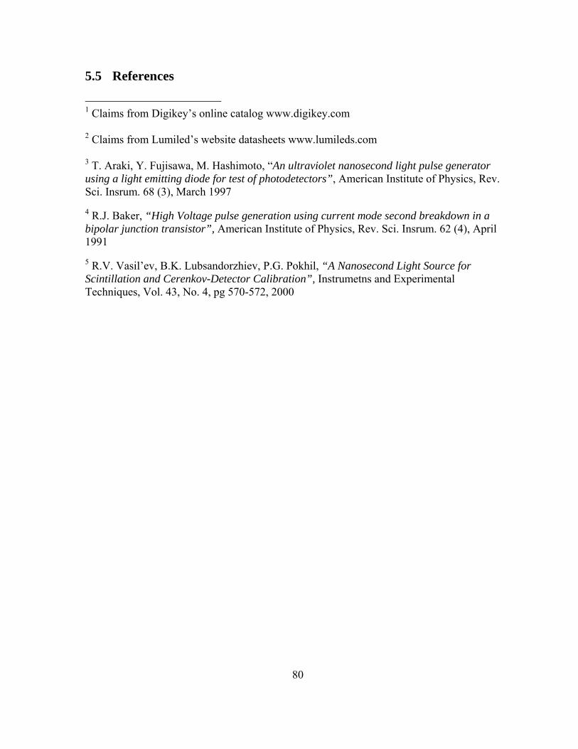
80

5.5 References

1 Claims from Digikey’s online catalog www.digikey.com 2 Claims from Lumiled’s website datasheets www.lumileds.com 3 T. Araki, Y. Fujisawa, M. Hashimoto, “An ultraviolet nanosecond light pulse generator using a light emitting diode for test of photodetectors”, American Institute of Physics, Rev. Sci. Insrum. 68 (3), March 1997 4 R.J. Baker, “High Voltage pulse generation using current mode second breakdown in a bipolar junction transistor”, American Institute of Physics, Rev. Sci. Insrum. 62 (4), April 1991 5 R.V. Vasil’ev, B.K. Lubsandorzhiev, P.G. Pokhil, “A Nanosecond Light Source for Scintillation and Cerenkov-Detector Calibration”, Instrumetns and Experimental Techniques, Vol. 43, No. 4, pg 570-572, 2000

81

Conclusion/Summary

The future tactical ocean environment will be increasingly complicated. In addition

to traditional communication links there will be a proliferation of unmanned vehicles in

space, in the air, on the surface, and underwater. To effectively utilize these systems

improvements in underwater communication systems are needed. Since radio wave do not

propagate in sea water, and acoustic communication systems are relatively low bandwidth

the possibility of high speed underwater optical communication systems are considered.

Applications for underwater optical communication systems include:

• Diver-to-diver communication links

• Diver-to-submarine links

• Submarine-to-UAV links

• Submarine-to-submarine links

• UAV-to-UAV links

• Submarine-to-satellite links

In this thesis there were two principle components a theoretical modeling effort of

underwater link budgets and an experimental effort to build LED based systems suitable for

underwater communications.

The model describing the inherent optical properties of ocean water, included:

• Absorption by Pure Seawater

• Absorption by Chlorophyll

• Absorption by Color Dissolved Organic Matter

• Scattering by Pure Seawater

• Scattering by Small & Large Particle

• Beam Spread through a horizontal water column

Chlorophyll is a major cause of loss in optical beam power. It is also very hard to find and

exact quantity of chlorophyll since it changes with location, time of day, season, and depth in

82

the water column. The assumption was made that the chlorophyll was distributed

homogeneously throughout the water column. Then, a theoretical link budget was

constructed and estimates for 3 underwater scenarios were found. These 3 scenarios were

and there corresponding link estimate are listed below:

• A blue/green LED based, bottom moored buoy system operating in relatively shallow

water. 1W LED - estimated link distance ~16 m

• A blue/green laser based system operating in deep clear ocean water with unlimited

power and size constraints. 10W Laser - estimated link distance ~425 m

• A power and size constrained, diode laser system suitable for small unmanned

underwater vehicle operation. 1W Laser - estimated link distance ~75 m

In the clearest of ocean conditions a link of ~425 m could be possible. Underwater optical

wireless links could be used in many applications with this distance. However, this estimate

is limited by not including scintillation caused by: temperature fluctuation, current and wind,

dispersion, and beam steering.

A figure of merit was also suggested to compare communications systems. It was

based on the platforms energy per bit, bit-rate length product, size, weight, and power usage.

Starting with the formula RxtEnvironmenTxSystem FOMFOMFOMFOM ⋅⋅= and plugging in:

⎟⎟⎠

⎞⎜⎜⎝

⎛

⋅⋅⋅⋅

⋅⋅⋅⋅⋅

Ω⋅⋅=

txTxTxTxTxsystem

PlatformPlatformplatfromOHPlatform

Txtx ApertureVolumeMassDensityAmps

aSurfaceAreVolumeMassDensityAmpHoursPower

Rangebits

FOM wsec

BackgroundSolaretcscatteringabsorptionWavelengthfFOMEnviron _),,( += K

⎟⎟⎠

⎞⎜⎜⎝

⎛

⋅⋅⋅⋅

⋅⋅⋅⋅⋅

⋅=

RxRxRxRxRxsystem

PlatformPlatformplatfromOHPlatform

reciever

FOVRx ApertureVolumeMassDensityAmps

aSurfaceAreVolumeMassDensityAmpHoursPower

AperturebitrateFOM w

83

Experimentally, the properties of LEDs when pulsed at high currents for

nanoseconds, was also examined. Using the secondary breakdown of an avalanche transistor,

a 4 ns pulse could be obtained from a LED that emitted over 109 photons per pulse. Though

we were limited by the EMCO high voltage dc-dc converter used to supply the 600V

potential to the collector lead, the potential of the circuit could still be seen. The higher

current caused the LED to produce Fabrey-Perot fringes, and it caused the wavelength to

shift ~10nm into lower wavelengths (higher energy).

An optical FM wireless LED system was constructed. The first generation circuit board

was made with the 4 ns circuit on it and deployed as the LED driver. The link was successful

in travel across the room (~30 ft) with just one lens on the receiver. Though the circuit

worked, it required too much power to drive the LED; 24 Volts to power the EMCO, 0 to 5 V

to control the output signal and 12 for the FM circuit.

A simpler and less power hungry driver circuit was implemented with the used of 3

stacked 74HC04 chips. With all the input pins soldiered together and all the output pins

soldiered and connected to the LED, the signal was a nice 3.5 volt square-wave output. A

new FM wireless board was made with the ability to have two way communications and

could run off a reasonable number of batteries. The FM circuit was successfully test

underwater with two-way voice communication.

Lastly, the open source free space project RONJA was constructed. While this was

initiated as an open source hardware project there were many challenges to overcome. The

availability of parts was an issue, and the design was not optimize and was less robust than

expected. While successful 10 Mbps operation was demonstrated and the Universal twisted

pair boards and transmitter boards worked to the standards, the receivers had problems

capturing the signal. This made the alignment process very difficult. Future work on receiver

design should be performed to make the system more resistant to pointing errors.

Underwater cases were designed and tested for use underwater. Using ABS piping

and couplers from Lowe’s Home Improvement, the optical lenses and circuits were placed

together for underwater experiments. It was found that using a lens as a window to provide

84

an air gaps for the collimating lenses was a better approach than to try to design for the water

environment directly. The lenses used in the transmitter allow the beam to stay well

collimated, after 140ft the beam diameter only doubled its original size.

To successfully deploying a free space underwater communication link in a real

world platform there are many more issues will have to be examined. For example, since

objects are in constant motion in the water, the transmitter and receiver will have to deploy

active feedback tracking in order to keep a stable link. After too long a distance, the beam

could be subject to beam steering due to index changes and currents. Other issues include

better packaging and reducing the size and energy requirements of the system.

Acoustical communications will still stand as the primary source of underwater

communications, but the research has shown optics may have a place in the underwater

environment. These products will take time and more research to develop, but the thesis

research presented has taken the first few steps in making underwater optical

communications a reality.

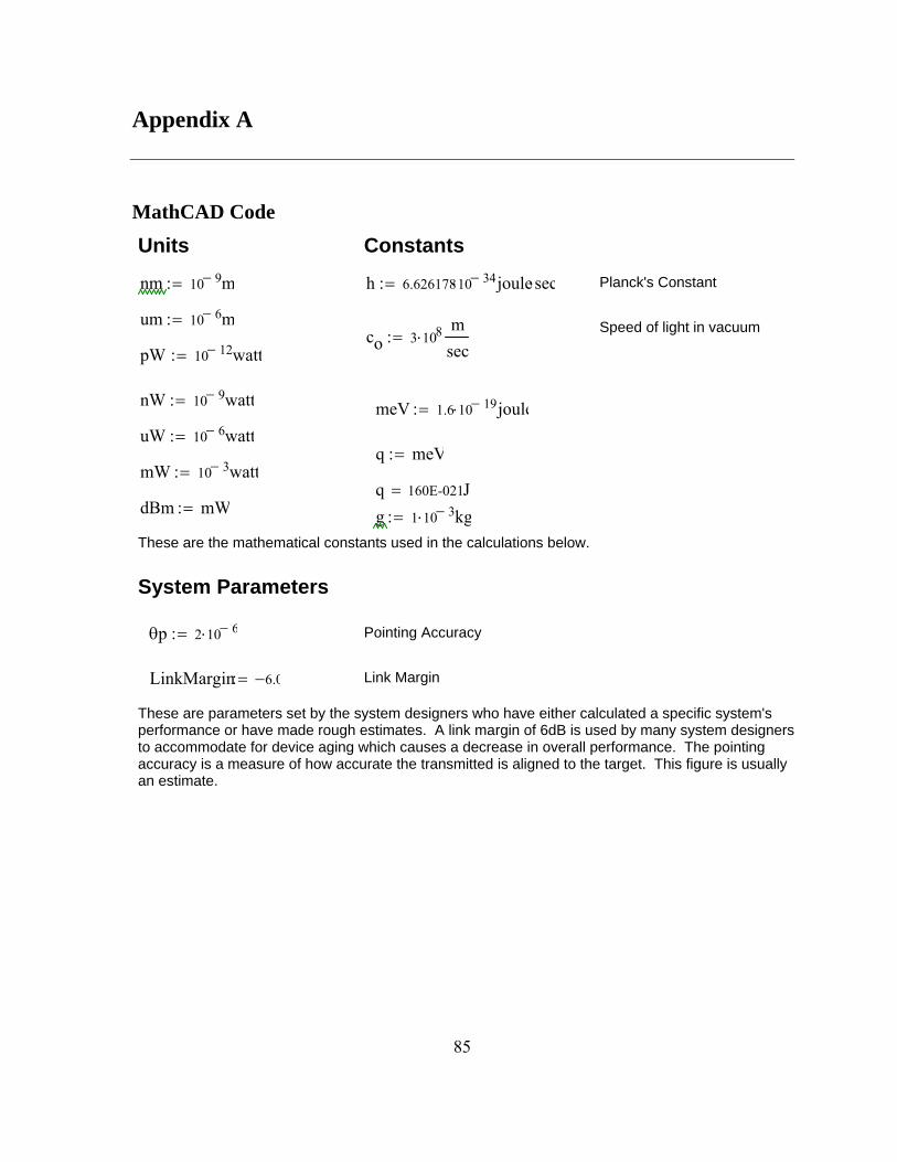
85

Appendix A

MathCAD Code

Units Constants

nm 10 9− m:= h 6.62617810 34−⋅ joulesec⋅:= Planck's Constant

um 10 6− m:= Speed of light in vacuum co 3 108⋅msec

:= pW 10 12− watt:=

nW 10 9− watt:= meV 1.6 10 19− joule⋅:=

uW 10 6− watt:= q meV:=

mW 10 3− watt:= q 160E-021J=

dBm mW:= g 1 10 3− kg⋅:=

These are the mathematical constants used in the calculations below.

System Parameters

θp 2 10 6−⋅:= Pointing Accuracy

LinkMargin 6.0−:= Link Margin

These are parameters set by the system designers who have either calculated a specific system's performance or have made rough estimates. A link margin of 6dB is used by many system designersto accommodate for device aging which causes a decrease in overall performance. The pointing accuracy is a measure of how accurate the transmitted is aligned to the target. This figure is usually an estimate.

86

Input Parameter Definitions and Limits

Depth Jerlov Water Type Selection Wavelength of Laser

Pure Water = 0 Type I = 1 Type 1A = 2 Type 1B = 3 Type II = 4 Type III = 5 Coastal 1 = 6 Coastal 2 = 7

Depth of transmitter in meters 200 λ≤ 800≤

Angle of Transmission

The angle at which the transmitter is pointing in degrees

0 = straight down 90 = completely horizontal 180 = straight up

Season of the Year Summer = 1 Fall = 2 Winter = 3 Spring = 4

87

Transmitter Parameters

λ 450nm:= Laser Wavelength

vo λ( )coλ

:= Optical Frequency

Pt 10mW:= Transmitter Power

Beam Divergence (rad) Div 1.5 10 6−⋅:=

lw 1:= Laser Line Width (nm)

Dt 5cm:= Transmitter Lens Diameter

pw := pulse width

θdiv 4λ

π Dt:= Transmitter Divergence

Gt 32

θdiv2:= Transmitter Gain

k 2π

λ:= Wavevector

NphPt

h vo λ( )⋅:= Photons per Bit from Transmitter

Lt 0.77:= Losses due to transmitter

k 13.963E+0061m

= Nph 22.637E+0151s

=

Each transmitter will consist of several parameters that will determine the performance of the system. The Transmitter Divergence and Gain were not used explicitly for my derivation. I was not comfortable with the "Gain" factor which really wasn't a gain(adding of photons) just a relationship between the beam divergence over the path length Lm. The use of the gain factor showed funny results. As I increased the power of the transmitter, it didn't seem to have much of an affect. Assumptions: Loss due to transmitter is 33%

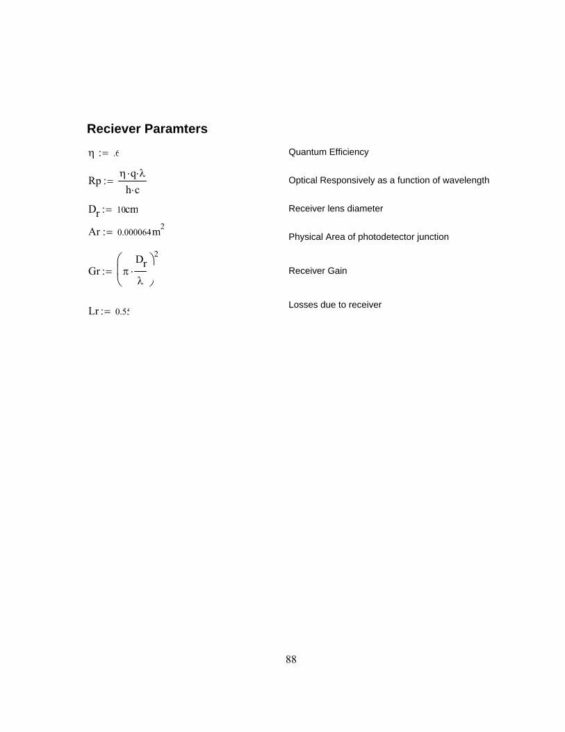
88

Reciever Paramters

η .6:= Quantum Efficiency

Rpη q⋅ λ⋅

h c⋅:= Optical Responsively as a function of wavelength

Dr 10cm:= Receiver lens diameter

Ar 0.000064m2⋅:= Physical Area of photodetector junction

Gr πDrλ

⋅⎛⎜⎝

⎞

⎠

2

:= Receiver Gain

Losses due to receiver Lr 0.55:=

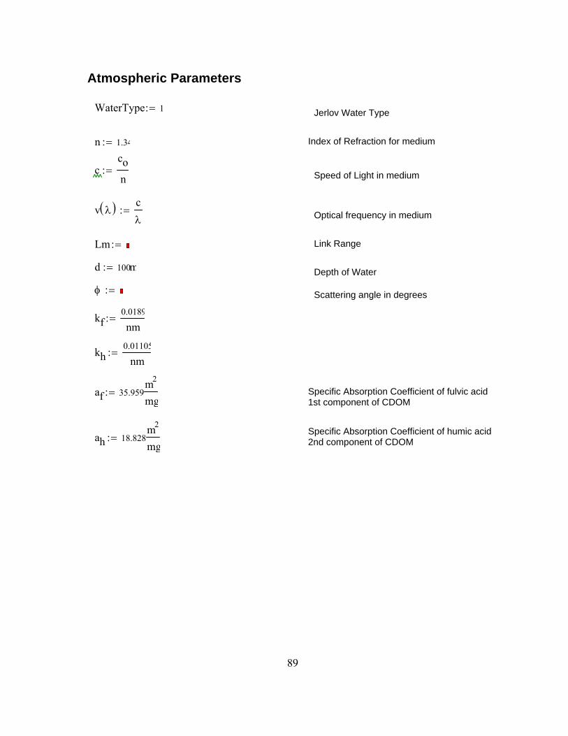
89

Atmospheric Parameters

WaterType 1:= Jerlov Water Type

n 1.34:= Index of Refraction for medium

ccon

:= Speed of Light in medium

v λ( ) cλ

:= Optical frequency in medium

Lm := Link Range

d 100m:= Depth of Water

φ := Scattering angle in degrees

kf0.0189

nm:=

kh0.01105

nm:=

af 35.959m2

mg:= Specific Absorption Coefficient of fulvic acid

1st component of CDOM

Specific Absorption Coefficient of humic acid 2nd component of CDOM ah 18.828

m2

mg:=

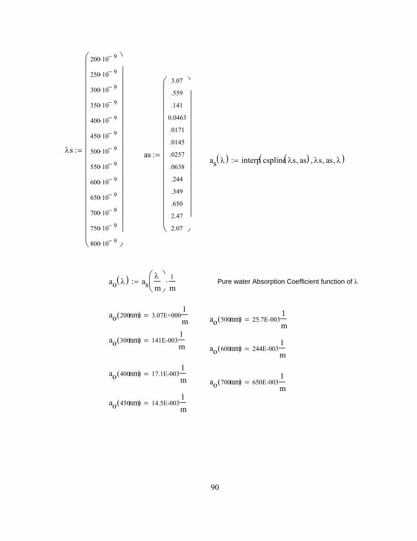
90

λs

200 10 9−⋅

250 10 9−⋅

300 10 9−⋅

350 10 9−⋅

400 10 9−⋅

450 10 9−⋅

500 10 9−⋅

550 10 9−⋅

600 10 9−⋅

650 10 9−⋅

700 10 9−⋅

750 10 9−⋅

800 10 9−⋅

⎛⎜⎜⎜⎜⎜⎜⎜⎜⎜⎜⎜⎜⎜⎜⎜⎜⎜⎜⎜⎝

⎞⎟⎟⎟⎟⎟⎟⎟⎟⎟⎟⎟⎟⎟⎟⎟⎟⎟

⎠

:= as

3.07

.559

.141

0.0463

.0171

.0145

.0257

.0638

.244

.349

.650

2.47

2.07

⎛⎜⎜⎜⎜⎜⎜⎜⎜⎜⎜⎜⎜⎜⎜⎜⎝

⎞⎟⎟⎟⎟⎟⎟⎟⎟⎟⎟⎟⎟⎟⎠

:= as λ( ) interp cspline λs as,( ) λs, as, λ,( ):=

ao λ( ) asλm

⎛⎜⎝

⎞⎠

1

m⋅:= Pure water Absorption Coefficient function of λ

ao 200nm( ) 3.07E+0001m

= ao 500nm( ) 25.7E-0031m

=

ao 300nm( ) 141E-0031m

= ao 600nm( ) 244E-003

1m

=

ao 400nm( ) 17.1E-0031m

= ao 700nm( ) 650E-003

1m

=

ao 450nm( ) 14.5E-0031m

=

91

Co WaterType( ) 0 WaterType 0if

0.03 WaterType 1if

0.1 WaterType 2if

0.4 WaterType 3if

1.25 WaterType 4if

3.0 WaterType 5if

9.0 WaterType 6if

12 WaterType 7if

:=

λc

300 10 9−⋅

350 10 9−⋅

400 10 9−⋅

450 10 9−⋅

475 10 9−⋅

500 10 9−⋅

525 10 9−⋅

550 10 9−⋅

600 10 9−⋅

650 10 9−⋅

675 10 9−⋅

700 10 9−⋅

750 10 9−⋅

800 10 9−⋅

⎛⎜⎜⎜⎜⎜⎜⎜⎜⎜⎜⎜⎜⎜⎜⎜⎜⎜⎜⎜⎜⎝

⎞

⎟⎟⎟⎟⎟⎟⎟⎟⎟⎟⎟⎟⎟⎟⎟⎟⎟⎟

⎠

:=

aco λ( )aclo

λm

⎛⎜⎝

⎞⎠

m:=

Cco 1mg

m3:=

ac

0.027

0.029

0.037

0.055

0.045

0.035

0.013

0.008

0.008

0.010

0.020

0.013

0.002

0

⎛⎜⎜⎜⎜⎜⎜⎜⎜⎜⎜⎜⎜⎜⎜⎜⎜⎝

⎞

⎟⎟⎟⎟⎟⎟⎟⎟⎟⎟⎟⎟⎟⎟

⎠

:= aclo λ( ) interp cspline λc ac,( ) λc, ac, λ,( ):=

Specific Absorption coefficient of chorophyll function of λ

92

Cc WaterType( )Co WaterType( ) mg

m3:= Total concentration of chlorophyll

Cf WaterType( ) 1.74098Cc WaterType( ) e0.12327

Cc WaterType( )

Cco⋅

⋅:=

Ch WaterType( ) 0.19334Cc WaterType( ) e0.12343

Cc WaterType( )

Cco⋅

⋅:=

bo λ( ) 5.826 10 3−⋅400nm

λ⎛⎜⎝

⎞⎠

4.322

⋅1

m:= Scattering Coefficient of pure water

bs λ( ) 1.1513400nm

λ⎛⎜⎝

⎞⎠

1.7⋅

m2

g:= Scattering Coefficient of small particles

bl λ( ) 0.3411400nm

λ⎛⎜⎝

⎞⎠

.3

⋅m2

g:= Scattering Coefficient of large particles

Csp WaterType( ) 0.01739g

mg⎛⎜⎝

⎞⎠

Cc WaterType( )⋅ e0.11631

Cc WaterType( )

Cco⋅

⋅:=

Clp WaterType( ) 0.76284g

mg⎛⎜⎝

⎞⎠

Cc WaterType( )⋅ e0.03092

Cc WaterType( )

Cco⋅

⋅:=

ps φ( ) 5.61746 e 2.957089− 10 2−⋅ φ

3

4⋅⎛⎜⎝

⎞⎠ 2.782943− 10 2−⋅ φ

6

4⋅⎛⎜⎝

⎞⎠+ 1.255406 10 3−⋅ φ

9

4⋅+ 2.155880− 10 5−⋅ φ

12

4⋅⎛⎜⎝

⎞⎠+ 1.356632 10 7−⋅ φ

15

4⋅⎛⎜⎝

⎞⎠+⋅:=

Concentration of humic acids

Concentration of fulvic acids

Concentration of small particles

Concentration of large particles

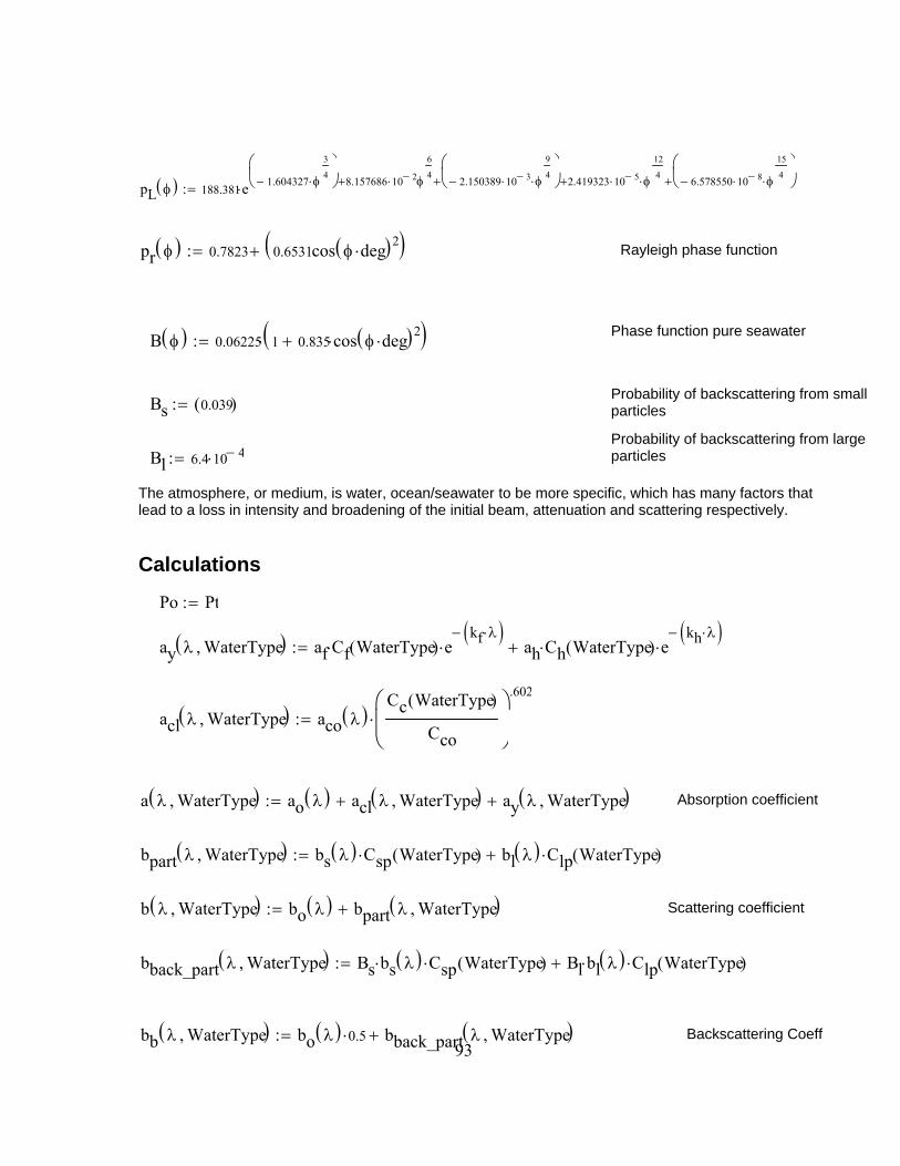
93

pL φ( ) 188.381e 1.604327− φ

3

4⋅⎛⎜⎝

⎞⎠ 8.157686 10 2−⋅ φ

6

4+ 2.150389− 10 3−⋅ φ

9

4⋅⎛⎜⎝

⎞⎠+ 2.419323 10 5−⋅ φ

12

4⋅+ 6.578550− 10 8−⋅ φ

15

4⋅⎛⎜⎝

⎞⎠+⋅:=

pr φ( ) 0.7823 0.6531cos φ deg⋅( )2( )+:= Rayleigh phase function

Phase function pure seawater B φ( ) 0.06225 1 0.835 cos φ deg⋅( )2⋅+( )⋅:=

Probability of backscattering from small particles Bs 0.039( ):=

Probability of backscattering from large particles Bl 6.4 10 4−⋅:=

The atmosphere, or medium, is water, ocean/seawater to be more specific, which has many factors that lead to a loss in intensity and broadening of the initial beam, attenuation and scattering respectively.

Calculations

Po Pt:=

ay λ WaterType,( ) af Cf WaterType( )⋅ ekf λ⋅( )−

⋅ ah Ch WaterType( )⋅ ekh λ⋅( )−

⋅+:=

acl λ WaterType,( ) aco λ( )Cc WaterType( )

Cco

⎛⎜⎝

⎞

⎠

.602

⋅:=

a λ WaterType,( ) ao λ( ) acl λ WaterType,( )+ ay λ WaterType,( )+:= Absorption coefficient

bpart λ WaterType,( ) bs λ( ) Csp WaterType( )⋅ bl λ( ) Clp WaterType( )⋅+:=

b λ WaterType,( ) bo λ( ) bpart λ WaterType,( )+:= Scattering coefficient

bback_part λ WaterType,( ) Bs bs λ( )⋅ Csp WaterType( )⋅ Bl bl λ( )⋅ Clp WaterType( )⋅+:=

bb λ WaterType,( ) bo λ( ) 0.5⋅ bback_part λ WaterType,( )+:= Backscattering Coeff

94

bh λ φ, WaterType,( ) bo λ( ) pr φ( ) bs λ( ) ps φ( )⋅ Csp WaterType( )⋅+ bl λ( ) pL φ( )⋅ Clp WaterType( )⋅+:=

Angular scattering Coeff

Attenuation Coefficient

LossLm Lm λ, WaterType,( ) e α λ WaterType,( )− Lm⋅ Dr2

Lm Div⋅ Dt+( )2⋅:=

Pr Lm λ,( ) Pt Lt( )⋅ LossLm Lm λ, WaterType,( )⋅ Lr( )⋅:=

LogPr Lm λ,( ) 10logPr Lm λ,( )

1W⎛⎜⎝

⎞⎠

:=

dBPr Lm λ,( ) LogPt LogLossLm Lm λ,( )+ LogGt+ LogGr+ LogLt+ LogLr+:=

α λ WaterType,( ) a λ WaterType,( ) b λ WaterType,( )+:=

Logarithmic Conversion to dB

LogPt 10logPt

1W⎛⎜⎝

⎞⎠

:=

LogGt 10log Gt( ):=

LogPt 0E+000=

LogGt 112.953E+000=

LogGr 10log Gr( ):= LogGr 115.964E+000=

LogLt 10log Lt( ):= LogLt 1.135E+000−=

LogLr 10log Lr( ):= LogLr 2.596E+000−=

LogLossLm Lm λ,( ) 10log LossLm Lm λ, WaterType,( )( ):=

95

Appendix B

Circuit Diagrams

Pulser Circuit

T. Araki, Y. Fujisawa, M. Hashimoto, “An ultraviolet nanosecond light pulse generator using a light emitting diode for test of photodetectors”, American Institute of Physics, Rev. Sci. Insrum. 68 (3), March 1997

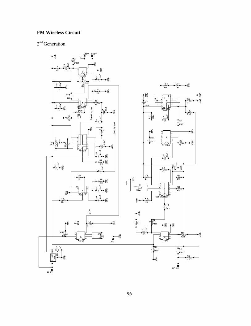
96

FM Wireless Circuit

2nd Generation

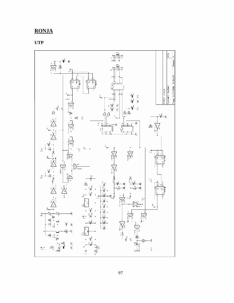
97

RONJA

UTP

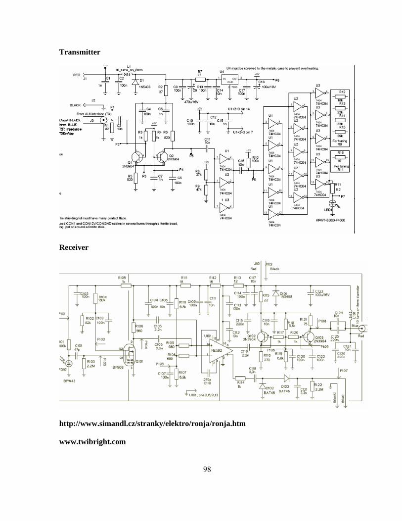
98

Transmitter

Receiver

http://www.simandl.cz/stranky/elektro/ronja/ronja.htm

www.twibright.com

99

Appendix C

Parts List

Pulser Board Device Value Package Quantity ZTX415 1 CAPACITOR 22p ceramic 50V 1 INDUCTOR 0.25u ceramic 50V 1 RESISTOR 51 250mW pref. metallic 1 RESISTOR 100 250mW pref. metallic 1 RESISTOR 1k 250mW pref. metallic 1 RESISTOR 60k 250mW pref. metallic 1

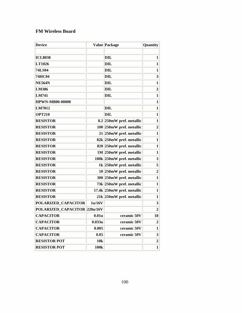
100

FM Wireless Board

Device Value Package Quantity ICL8038 DIL 1LT1026 DIL 1 74LS04 DIL 1 74HC04 DIL 3 NE564N DIL 1 LM386 DIL 2 LM741 DIL 1 HPWN-MB00-00000 1 LM7812 DIL 1 OPT210 DIL 1 RESISTOR 8.2 250mW pref. metallic 1 RESISTOR 100 250mW pref. metallic 2 RESISTOR 21 250mW pref. metallic 1 RESISTOR 82k 250mW pref. metallic 1 RESISTOR 820 250mW pref. metallic 1 RESISTOR 1M 250mW pref. metallic 1RESISTOR 100k 250mW pref. metallic 3RESISTOR 1k 250mW pref. metallic 5RESISTOR 10 250mW pref. metallic 2RESISTOR 300 250mW pref. metallic 1RESISTOR 73k 250mW pref. metallic 1RESISTOR 17.4k 250mW pref. metallic 1RESISTOR 21k 250mW pref. metallic 1POLARIZED_CAPACITOR 1u/16V 3 POLARIZED_CAPACITOR 220u/16V 2 CAPACITOR 0.01u ceramic 50V 18CAPACITOR 0.033u ceramic 50V 2CAPACITOR 0.005 ceramic 50V 1CAPACITOR 0.05 ceramic 50V 3RESISTOR POT 10k 2RESISTOR POT 100k 1

101

RONJA Boards UTP

Device Value Package Quantity 20F001N RJ45 FILTER 174HC74N DIL 2 74HC04 DIL 1 74HC132 DIL 2 74HC14 DIL 2 MC3487 DIL 1 MC3486 DIL 1 IN4148 DIODE 4 2N3904 DIODE 2 7805 & 7812 VOLT REG 1/each RESISTOR 47k 250mW pref. metallic 1 RESISTOR 220 250mW pref. metallic 6 RESISTOR 50 250mW pref. metallic 4 RESISTOR 10k 250mW pref. metallic 1 RESISTOR 82 250mW pref. metallic 1 RESISTOR 3.3k 250mW pref. metallic 2RESISTOR 100k 250mW pref. metallic 1RESISTOR 1k 250mW pref. metallic 3RESISTOR 1.8k 250mW pref. metallic 1RESISTOR 120k 250mW pref. metallic 1RESISTOR 23 250mW pref. metallic 1RESISTOR 1.2k 250mW pref. metallic 1INDUCTOR 330u Wire wrapped 1POLARIZED_CAPACITOR 1000u/50V 2 POLARIZED_CAPACITOR 220u/16V 1 CAPACITOR 0.1u ceramic 50V 20CAPACITOR 100p ceramic 50V 4CAPACITOR 47p ceramic 50V 2CAPACITOR 180p ceramic 50V 1CAPACITOR 10n ceramic 50V 2CAPACITOR 220n ceramic 50V 1CAPACITOR 150p ceramic 50V 1RED,GREEN,YELLOW LED 1/each

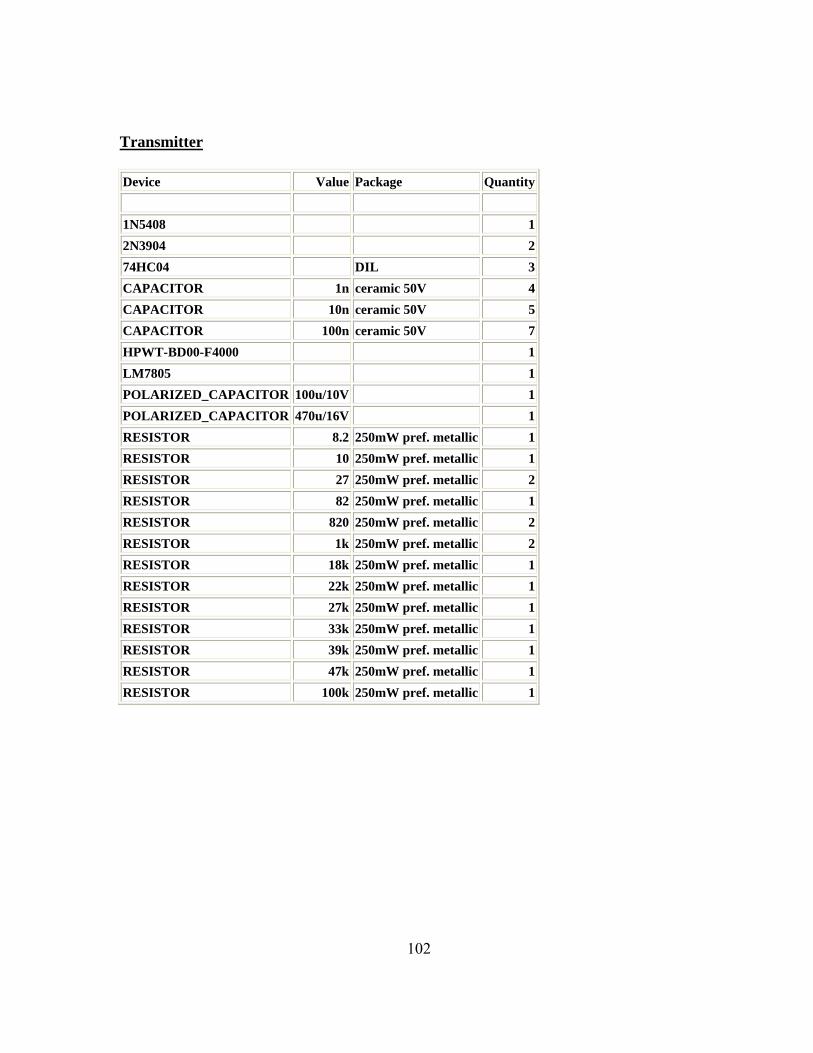
102

Transmitter Device Value Package Quantity 1N5408 1 2N3904 2 74HC04 DIL 3 CAPACITOR 1n ceramic 50V 4 CAPACITOR 10n ceramic 50V 5 CAPACITOR 100n ceramic 50V 7 HPWT-BD00-F4000 1 LM7805 1 POLARIZED_CAPACITOR 100u/10V 1 POLARIZED_CAPACITOR 470u/16V 1 RESISTOR 8.2 250mW pref. metallic 1 RESISTOR 10 250mW pref. metallic 1 RESISTOR 27 250mW pref. metallic 2 RESISTOR 82 250mW pref. metallic 1 RESISTOR 820 250mW pref. metallic 2 RESISTOR 1k 250mW pref. metallic 2 RESISTOR 18k 250mW pref. metallic 1 RESISTOR 22k 250mW pref. metallic 1 RESISTOR 27k 250mW pref. metallic 1 RESISTOR 33k 250mW pref. metallic 1 RESISTOR 39k 250mW pref. metallic 1 RESISTOR 47k 250mW pref. metallic 1 RESISTOR 100k 250mW pref. metallic 1

103

Receiver

Device Value Package Quantity 1N5408 1 2N3904 2 BAT46 2 BF908 1 BPW43 1 CAPACITOR 47p ceramic 50V 1 CAPACITOR 270p ceramic 50V 1 CAPACITOR 1n ceramic 50V 1 CAPACITOR 2.2n ceramic 50V 3 CAPACITOR 3.3n ceramic 50V 1 CAPACITOR 10n ceramic 50V 7 CAPACITOR 100n ceramic 50V 10 CAPACITOR 220n ceramic 50V 3 NE592 DIL14 1 POLARIZED_CAPACITOR 100u/16V 1 RESISTOR 12 250mW pref. metallic 1 RESISTOR 18 250mW pref. metallic 2 RESISTOR 22 250mW pref. metallic 1 RESISTOR 75 250mW pref. metallic 1 RESISTOR 180 250mW pref. metallic 1 RESISTOR 220 250mW pref. metallic 1 RESISTOR 270 250mW pref. metallic 2 RESISTOR 330 250mW pref. metallic 1 RESISTOR 390 250mW pref. metallic 1 RESISTOR 470 250mW pref. metallic 1 RESISTOR 560 250mW pref. metallic 2 RESISTOR 680 250mW pref. metallic 3 RESISTOR 820 250mW pref. metallic 1 RESISTOR 1k 250mW pref. metallic 5 RESISTOR 1.2k 250mW pref. metallic 1 RESISTOR 1.5k 250mW pref. metallic 1 RESISTOR 1.8k 250mW pref. metallic 1 RESISTOR 6.8k 250mW pref. metallic 4 RESISTOR 82k 250mW pref. metallic 2

104

RESISTOR 100k 250mW pref. metallic 3 RESISTOR 120k 250mW pref. metallic 1 RESISTOR 180k 250mW pref. metallic 1 RESISTOR 2.2M 250mW pref. metallic 1