MARITIME NAVIGATION AND CONTACT AVOIDANCE THROUGH

The Pennsylvania State University

The Graduate School

College of Engineering

MARITIME NAVIGATION AND CONTACT AVOIDANCE

THROUGH REINFORCEMNT LEARNING

A Thesis in

Computer Science and Engineering

by

Steven Lee Davis

© 2019 Steven Lee Davis

Submitted in Partial Fulfillment

of the Requirements

for the Degree of

Master of Science

May 2019

ii

The thesis of Steven Lee Davis was reviewed and approved* by the following:

Vijaykrishnan Narayanan

Distinguished Professor of Computer Science and Engineering

Thesis Co-Advisor

John Sustersic

Assistant Research Professor, Penn State Applied Research Lab

Thesis Co-Advisor

John Sampson

Assistant Professor of Computer Science and Engineering

Chitaranjan Das

Distinguished Professor of Computer Science and Engineering

Head of the Department of Computer Science and Engineering

*Signatures are on file in the Graduate School

iii

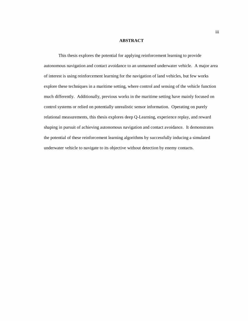
ABSTRACT

This thesis explores the potential for applying reinforcement learning to provide

autonomous navigation and contact avoidance to an unmanned underwater vehicle. A major area

of interest is using reinforcement learning for the navigation of land vehicles, but few works

explore these techniques in a maritime setting, where control and sensing of the vehicle function

much differently. Additionally, previous works in the maritime setting have mainly focused on

control systems or relied on potentially unrealistic sensor information. Operating on purely

relational measurements, this thesis explores deep Q-Learning, experience replay, and reward

shaping in pursuit of achieving autonomous navigation and contact avoidance. It demonstrates

the potential of these reinforcement learning algorithms by successfully inducing a simulated

underwater vehicle to navigate to its objective without detection by enemy contacts.

iv

TABLE OF CONTENTS

LIST OF FIGURES ................................................................................................................. vi

LIST OF TABLES ................................................................................................................... vii

ACKNOWLEDGEMENTS ..................................................................................................... viii

Chapter 1 Introduction ............................................................................................................ 1

Related Work ................................................................................................................... 3 UUV Control ............................................................................................................ 3 UUV Navigation ...................................................................................................... 5

Chapter 2 Background ............................................................................................................ 7

Reinforcement Learning .................................................................................................. 7 Markov Decision Processes ............................................................................................. 9

The Agent and Environment .................................................................................... 9 States, Actions, and Rewards ................................................................................... 11

Cumulative Reward, Value Functions, and Policies........................................................ 12 Value as a Function of State .................................................................................... 13 Value as a Function of State and Action .................................................................. 14 Policies ..................................................................................................................... 14 Policy Optimality ..................................................................................................... 16

Reward Functions ............................................................................................................ 16

Chapter 3 Algorithms ............................................................................................................. 18

Exploitation-Exploration Tradeoff .................................................................................. 18 Epsilon-Greedy Policies........................................................................................... 18

Algorithm Characteristics ................................................................................................ 19 Model and Model-Free Algorithms ......................................................................... 19 On-Policy and Off-Policy Algorithms ..................................................................... 20 Dynamic Programming, Monte-Carlo, and Temporal Differencing Algorithms .... 20

Q-Learning ....................................................................................................................... 21 Convergence Guarantees ......................................................................................... 23 Issues with Tabular Q-Learning............................................................................... 23

Deep Q-Learning ............................................................................................................. 24 Catastrophic Forgetting ............................................................................................ 25 Experience Replay ................................................................................................... 25

Chapter 4 Problem and Approach........................................................................................... 28

Unmanned Underwater Vehicles (UUVs) ....................................................................... 28 Limitations of a UUV ...................................................................................................... 29 Assumptions of the Simulated UUV ............................................................................... 30 Simulated Environment ................................................................................................... 31

v

Additional Parameters .............................................................................................. 34 State Representation................................................................................................. 35 Reward Architecture ................................................................................................ 35

Chapter 5 Implementation and Evaluation ............................................................................. 37

Baseline – Random Walk ................................................................................................ 37 General Simulation Dynamics ......................................................................................... 38 Tabular Q-Learning ......................................................................................................... 39 Deep Q-Learning ............................................................................................................. 39

Network Architecture............................................................................................... 40 Performance ............................................................................................................. 40 Discussion ................................................................................................................ 41

Deep Q-Learning with Experience Replay ...................................................................... 42 Network Architecture............................................................................................... 42 Performance ............................................................................................................. 43 Discussion ................................................................................................................ 44 Example Behavior .................................................................................................... 45 Modeling Sensor Noise ............................................................................................ 50

Deep Q Learning with Experience Replay and Reward Shaping .................................... 51 Network Architecture............................................................................................... 52 Performance ............................................................................................................. 53 Discussion ................................................................................................................ 54 Example Behavior .................................................................................................... 54 Catastrophic Forgetting from Extreme Shaping and Small Memory ...................... 60

Chapter 6 Discussion .............................................................................................................. 62

Possible Future Work....................................................................................................... 63 Use of Expanded Information .................................................................................. 63 Evaluation of Additional Algorithms....................................................................... 64 Application to 3D Simulation .................................................................................. 65 Transfer Learning to Real-World Agent .................................................................. 65

Chapter 7 Conclusion ............................................................................................................. 66

Bibliography ............................................................................................................................ 67

Appendix A Summary of Notation and Acronyms ................................................................ 70

Appendix B Code ................................................................................................................... 72

ReinforcementLearningModule.py .......................................................................... 72 DeepQLearningWithExperienceReplayModule.py ................................................. 74

vi

LIST OF FIGURES

Figure 2-1: Markov Decision Process [16] ............................................................................. 9

Figure 3-1: Epsilon Greedy Q-Learning Pseudocode ............................................................. 23

Figure 3-2: Epsilon Greedy Deep Q-Learning Pseudocode ................................................... 24

Figure 3-3: Epsilon Greedy Deep Q-Learning with Experience Replay Pseudocode ............ 26

Figure 4-1: An Unmanned Underwater Vehicle (UUV) [29] ................................................. 28

Figure 4-2: Example Initialized Simulated Environment ....................................................... 32

Figure 4-3: Example Initialized Simulated Environment Movement Progression ................. 33

Figure 4-4: Contacts with Hitboxes (25, 50, and 100 units) ................................................... 34

Figure 4-5: Instantaneous State Vector................................................................................... 35

Figure 5-1: Performance – Random Navigation ..................................................................... 38

Figure 5-2: Performance – Deep Q-Learning ......................................................................... 41

Figure 5-3: Performance – Deep Q-Learning with Experience Replay ................................. 44

Figure 5-4: Recognize Potential Collision – Deep Q-Learning with Experience Replay ...... 46

Figure 5-5: Perform Trajectory Correction – Deep Q-Learning with Experience Replay ..... 47

Figure 5-6: Continue on Course – Deep Q-Learning with Experience Replay ...................... 48

Figure 5-7: Collision Avoidance – Deep Q-Learning with Experience Replay ..................... 50

Figure 5-8: Performance – Deep Q-Learning with Experience Replay with Sensor Noise ... 51

Figure 5-9: Performance – Deep Q-Learning with Experience Replay and Reward

Shaping ............................................................................................................................ 53

Figure 5-10: Stop and Adjust – Deep Q-Learning with Experience Replay and Reward

Shaping ............................................................................................................................ 55

Figure 5-11: Continue through Close Encounter – Deep Q-Learning with Experience

Replay and Reward Shaping ............................................................................................ 56

Figure 5-12: Complex Trajectory Correction – Deep Q-Learning with Experience Replay

and Reward Shaping ........................................................................................................ 58

Figure 5-13: Performance – Catastrophic Forgetting with Experience Replay ...................... 61

vii

LIST OF TABLES

Table 4-1: UUV Action Space ................................................................................................ 30

Table 4-2: Information Available to UUV ............................................................................. 31

Table 5-1: Reward Shaping Schedule..................................................................................... 52

Table 5-2: Reward Shaping Schedule – Catastrophic Forgetting ........................................... 60

Table A-1: Summary of Notation ........................................................................................... 70

Table A-2: Summary of Acronyms ........................................................................................ 71

viii

ACKNOWLEDGEMENTS

I would like to thank my Thesis Committee: Vijay Narayanan, John Sustersic, and Jack

Sampson; without their support this thesis would not have been possible.

Thank you, Dr. John Sustersic and my fellow students at the Applied Research Lab, Eric

Homan, Ken Hall, and Sarah McClure, for providing immense support of this thesis. I have

learned so much by working with you.

Thank you, Dr. Vijay Narayanan, my co-advisor from the Penn State College of

Engineering, for providing invaluable guidance and support throughout my academic career.

Thank you, Dr. Jack Sampson, for supporting of my graduate education when I needed it

most.

Finally, thank you to my family and friends who have pushed and motivated me

throughout my academic career.

This work was supported in part by C-BRIC, one of six centers in JUMP, a

Semiconductor Research Corporation (SRC) program sponsored by DARPA. The findings and

conclusions expressed in this thesis are my opinions and are not reflective of those of any funding

body.

1

Chapter 1

Introduction

The field of Artificial Intelligence has exploded in recent years. Today, tools such as

smart voice assistants, intelligent song/movie recommendation systems, and various smart home

devices are common in many individuals’ lives. Tomorrow, technologies such as self-driving

cars, package delivery drones, and robot assistants in the home might seem just as common. All

of these systems have one thing in common—they learn from data. Such applications of artificial

intelligence and machine learning have and will continue to have a profound impact on our

lifestyle.

Machine learning systems often process tremendous amounts of data to provide us with

the recommendations, answers, or assistance we require. Many companies make a fortune tuning

these algorithms for the benefit of their consumers. The algorithms ingest data, learn from it, and

make decisions in some way. This poses the question, what is learning?

One natural way to view learning and intelligence is through the process of trial and

error. Intelligent beings are able to distinguish between the actions and situations of successful

and of failed tasks. A parent might scold a child for inappropriate decisions or reward them for

doing something correctly. As the child grows and develops, the role of the parent becomes less

necessary, as the child learns new ideas and tasks on their own, being able to discern correct from

incorrect without feedback from an explicit teacher. Learning through experience, through trial

and error rather than from labelled examples, and through rewards and penalties is an example of

reinforcement learning, one domain of machine learning.

In reinforcement learning, there need not be an explicit expert teacher. Rather, the agent

of learning explores the world, and through the receipt of rewards and/or penalties, learns to

2

accomplish some task. Even with no prior knowledge, just through simple interactions, it may be

possible to learn extremely complex tasks.

One task of interest to the United States Navy and other organizations is that of

navigating unmanned underwater vehicles whilst remaining undetected by external parties. This

thesis will explore, in simulation, applying principles of reinforcement learning to accomplish this

unique task.

Recent advances in machine learning motivate the completion of this thesis. The advent

of deep learning and deep neural networks [1], [2] in domains such as image classification have

set a new state-of-the-art for many classification and regression tasks. The use of neural networks

for function approximation has proven to provide extreme accuracy in some domains and powers

deep reinforcement learning in this one.

Additionally, advances in reinforcement learning have incited renewed interest in the

field as a subdomain of machine learning. Advances in many game applications by Google

DeepMind such as surpassing human-level performance playing Atari games [3], AlphaGo

beating a world champion at the complex game of Go [4], and then later AlphaGo Zero doing so

again, without the use of any human knowledge [5] have revitalized interest in reinforcement

learning. Still, applying reinforcement learning in other applications, especially those with

continuous state representation or those lacking complete knowledge remains a challenge.

The remainder of this thesis will continue as follows. First, the current state-of-the-art

work being done with reinforcement learning and unmanned/autonomous underwater vehicles

will be discussed. Then, a background of the mathematical model supporting reinforcement

learning and common algorithms to solve the reinforcement learning problem will be reviewed.

Next, the specifics of the unmanned underwater vehicle navigation and contact avoidance

3

problem will be discussed. Finally, reinforcement learning algorithms will be implemented and

tested against the problem in this context, followed by a discussion of the results.

Related Work

As unmanned/autonomous vehicles are of great interest to many organizations, military,

government, environmental, and industry alike, several researchers have examined the application

of reinforcement learning to them in various contexts, primarily control and navigation.

UUV Control

Several works have examined applying reinforcement learning to the control systems of

unmanned/autonomous underwater vehicles. In this sense, the reinforcement learning algorithms

are not being used for navigation planning, but rather enable the vehicle to accurately follow a

pre-determined trajectory. In these cases, reinforcement learning techniques are being used to

eliminate the complexity of the UUV control/dynamics model, or the complexity introduced by

random disturbances such as currents and waves.

Yu, et. al. [6] examines using deep reinforcement learning techniques to control a UUV

and overcome random disturbances. This work supposes a pre-determined linear trajectory. The

goal was to use reinforcement learning, in simulation, to stabilize the UUV and use its low-level

controls to follow the pre-determined trajectory and overcome random disturbances. This work

used an actor-critic model to suggest and evaluate actions, where the error was represented as the

absolute deviation from the pre-determined trajectory. Yu, et. al. suggests that reinforcement

learning can provide better control performance over classic control theories.

4

Carlucho, et. al. [7] also examined the problem of low-level control of autonomous

underwater vehicles. This work aimed to apply another actor-critic architecture to map raw

sensory information to low-level commands for a UUV’s thrusters. The authors were successful

in applying their algorithm in a wet, real-world environment. The algorithm was able to

overcome, in simulation, and to some extent in the wet environment, disturbances and model

uncertainty to match desired linear and angular velocities as specified by the operator.

Finally, Wu, et. al. [8] examines the more niche task of depth control. Their aim was to

use reinforcement learning to control a UUV to maintain constant depth, or to follow a specific

depth trajectory over time. Also tested only in simulation, the authors used a deep deterministic

policy gradient approach to outperform, in simulation, two model-based control policies. Aimed

primarily for deep sea depth tracking, this work showed promise for the application of

reinforcement learning to more specific areas of control.

Each of these works seeks to pass control from traditional, complicated control models to

reinforcement learning models that attempt to account for model uncertainty and random

disturbances with the goal of matching desired velocity and positions specified by a controller.

This thesis will seek to extend these works by focusing on navigational planning. [6]–[8] have

demonstrated that state-of-the-art deep reinforcement learning techniques can be used to induce

the UUV to accurately adjust its velocities and positioning in accordance with the commands of

the operator, overcoming model uncertainty and natural disturbances in the water. Having

achieved this, this thesis will assume accurate control of the vehicle and explore applying

reinforcement learning to achieve online navigation in search of a specific objective in an

unknown environment.

5

UUV Navigation

In addition to control theory, other works have explored the task of UUV navigation via

the exploitation of reinforcement learning.

Gaskett, et. al. [9] seeks to bridge control and navigation by applying reinforcement

learning to the problem of controlling thrusters in response to commands and sensors. This work

examined a specific UUV owned by the Australian National University primarily used for

cataloging reefs and other geological features. In simulation, with knowledge of the exact

location of the goal, and in the absence of any obstacles, the agent was given positive reward for

each timestep which moved it closer to its goal. With successful navigation to the goal, this work

showed early promise of connecting control and navigation via reinforcement learning.

An older work by El-Fakdi, et. al. [10] forgoes value approximation techniques and

attempts to use policy search methods to navigate a UUV to an objective in simulation and in the

absence of obstacles. This work assumes only four inputs, the x/y distance to the objective, and

the x/y velocity of the agent. Using an 11-neuron network, the agent navigates to the objective.

Although very limited in complexity, this paper demonstrates the feasibility for reinforcement

learning in a maritime navigation planning context.

Wang, et. al. [11] approaches the task of navigation from a different perspective. Rather

than directly controlling a singular UUV, the work assumes a network of many UUVs which can

navigate between many, fixed access points. Rather than a trajectory specifying granular control,

a trajectory specifies an ordering of waypoints for each UUV to visit. The goal of the work was

to maximize the area of the region explored by the network of UUVs. Reinforcement learning

was induced with state representing the current collected field knowledge, and actions specifying

which waypoint to visit next, with the goal of maximizing information collected throughout the

trajectories.

6

Finally, Sun, et. al. [12] (February 2019) examines the context of navigation most similar

to this thesis, using reinforcement learning techniques, in simulation, for motion planning in a

mapless environment. This work assumes a two-dimensional model of the environment, where

the goal is to map sensor data to the thrusters of the UUV. Active sonar sensors enable the agent

to obtain accurate information of nearby obstacles that could present potential collisions. Having

knowledge of the distance to static obstacles and the absolute coordinates of both itself and the

objective, this work uses a proximal policy optimization technique to teach the agent to avoid

collisions and navigate to the objective with high accuracy. This thesis will seek to extend the

scope of this work by incorporating dynamic (moving) obstacles to the environment, while also

reducing the sensory input information available to the learning algorithm.

Each of these works operates under the assumption of either no obstacles, or static

obstacles in the world. Additionally, many offer unrealistic sensor information, in that the UUV

may not have accurate knowledge of its own absolute coordinates, nor the absolute coordinates of

the obstacles it seeks to avoid. This thesis seeks to extend the scope of the state-of-the art works

in unmanned/autonomous underwater vehicle navigation through the incorporation of dynamic,

moving, wide-range contacts and a reduction in the information provided by on-board sensors.

7

Chapter 2

Background

In this chapter, we will first explain the intuition behind reinforcement learning before

formalizing the framework through Markov decision processes.

Reinforcement Learning

Reinforcement learning (RL) is a computational approach to learning from interaction

with one’s environment. Instead of exploiting an explicit teacher, reinforcement learning

algorithms seek to derive a connection between cause and effect: between the actions an agent

takes, and the resultant situations and rewards experienced because of those actions. At the core,

reinforcement learning is defined as the process of an agent taking actions in an environment, as

to maximize some sense of cumulative reward. The goal is to create a mapping of states to

actions, called a policy, such that the amount of reward achieved over time is at maximum. The

complexity of this analysis arises in that the agent needs to become aware of how the

environment responds to its actions. Further, the actions taken affect not only the instantaneous

reward received, but also the next state, and thus all future states and rewards.

Reinforcement learning is often thought of as a third branch of machine learning, distinct

from both supervised learning and unsupervised learning. In supervised learning, labelled

training examples inform an algorithm to best select a choice when given unseen, future test

samples. RL lacks such labelled examples. Reinforcement learning evaluates the consequence of

actions in a changing environment rather than simply informing the selection of a class, and

therefore must seek out examples for itself, through the process of exploration. Given this lack of

8

labelled training data, one might think that reinforcement learning could be a subdomain of

unsupervised learning. However, RL does not explicitly seek to find hidden structure in a fixed

dataset, as is common in unsupervised learning. Rather, its goal is to understand its environment

and maximize cumulative reward from a set of actions.

Reinforcement learning involves an explicit goal that one wishes to achieve, the ability to

sense information about one’s environment, and the ability to take actions to modify the

environment in pursuit of the goal. The primary issue of reinforcement learning is the

understanding of delayed reward. Agents must understand that taking potentially sub-optimal

tasks at one point in time may create opportunities for even greater reward (as defined by the

goal) at a later point in time.

This phenomenon leads to the tradeoff between exploration and exploitation. In order to

achieve its goal, a reinforcement learning agent must exploit its current knowledge. However, in

order to build that knowledge, it must explore unknown, possibly ineffective actions. Neither

pure exploitation nor pure exploration may be pursued without failing to achieve the goal.

Further, a common theme in reinforcement learning is some degree of uncertainty about

the environment. These, called model free, problems require the agent to build up knowledge not

only of cause and effect, but also of what situations ae even possible to encounter in an initially

unknown environment.

In its purest form, reinforcement learning agents learn from a blank slate, or tabula rasa,

with no prior experience imposed, however, techniques exist for introducing such prior

knowledge to improve performance or shorten training times in some domains [13]–[15].

9

Markov Decision Processes

The reinforcement learning problem is almost universally formalized as a Markov

decision process (MDP). Thus, solving (or finding an approximate solution to) this formalization

of the reinforcement learning problem, solves (or finds an approximate solution to) the

reinforcement learning problem itself.

The MDP models sequential decision making, where decisions impact not only

immediate rewards, but also the states available in the future, and as such, the rewards available

in the future. Given this form of decision making which affects future reward, there exists an

important tradeoff between the value of immediate rewards and the value of future rewards.

The Agent and Environment

A Markov decision process is formalized as follows: an agent, beginning in a state, takes

an action in its environment, and thus receives a scalar reward and transitions to a new state. This

process is visually depicted in Figure 2-1.

The agent and environment interact at discrete timesteps, resulting in a trajectory of state-

action-reward tuples.

Figure 2-1: Markov Decision Process [16]

10

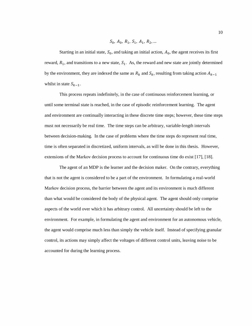
𝑆0, 𝐴0, 𝑅1, 𝑆1, 𝐴1, 𝑅2, …

Starting in an initial state, 𝑆0, and taking an initial action, 𝐴0, the agent receives its first

reward, 𝑅1, and transitions to a new state, 𝑆1. As, the reward and new state are jointly determined

by the environment, they are indexed the same as 𝑅𝑘 and 𝑆𝑘, resulting from taking action 𝐴𝑘−1

whilst in state 𝑆𝑘−1.

This process repeats indefinitely, in the case of continuous reinforcement learning, or

until some terminal state is reached, in the case of episodic reinforcement learning. The agent

and environment are continually interacting in these discrete time steps; however, these time steps

must not necessarily be real time. The time steps can be arbitrary, variable-length intervals

between decision-making. In the case of problems where the time steps do represent real time,

time is often separated in discretized, uniform intervals, as will be done in this thesis. However,

extensions of the Markov decision process to account for continuous time do exist [17], [18].

The agent of an MDP is the learner and the decision maker. On the contrary, everything

that is not the agent is considered to be a part of the environment. In formulating a real-world

Markov decision process, the barrier between the agent and its environment is much different

than what would be considered the body of the physical agent. The agent should only comprise

aspects of the world over which it has arbitrary control. All uncertainty should be left to the

environment. For example, in formulating the agent and environment for an autonomous vehicle,

the agent would comprise much less than simply the vehicle itself. Instead of specifying granular

control, its actions may simply affect the voltages of different control units, leaving noise to be

accounted for during the learning process.

11

States, Actions, and Rewards

In a finite Markov decision process, the set of possible states (𝒮) and the set of possible

actions (𝒜) that may be taken in each of these states is finite. In an infinite MDP, this

assumption is relaxed [19]. Note that even in a finite MDP, the number of time steps experienced

may be infinite, and an agent may operate indefinitely, so long as the number of states and actions

are bounded.

For each state-action pair (taking an action in a state), the Markov decision process

formulates that there exists a probability distribution over the resultant state and reward.

𝑃(𝑠′, 𝑟 | 𝑠, 𝑎) = Pr{𝑆𝑡 , = 𝑠′, 𝑅𝑡 = 𝑟′ | 𝑆𝑡−1 = 𝑠, 𝐴𝑡−1 = 𝑎}

That is, state-action pairs are not necessarily deterministic; they are stochastic. The

Markov decision process model inherently accounts for some uncertainty. Rather, taking action 𝑎

while in state 𝑠 leads the agent to the new state 𝑠′ with reward 𝑟, not with certainty, but rather

with the probability 𝑃(𝑠′, 𝑟 | 𝑠, 𝑎).

Markov Property

Importantly, note that the current state of an MDP completely characterizes the process.

That is, a property of the MDP is that any information not contained in the state does not affect

the conditional state transition probability, and as such should have no impact on future

interactions between the agent and the environment. The process is memoryless. This notion is

defined as the Markov property.

The Markov property importantly places a restriction on the definition of state. In an

idealized MDP, the state must contain all relevant information of past interactions that might in

any way affect the future.

12

The Markov property makes it more convenient to apply reinforcement learning

algorithms to problems with complete information. Complete information is a property in which

total knowledge of the environment is known, and the current state provides all necessary

information of what has happened in the past. Games such as backgammon, chess, and Go

respect this property and as such have been solved to a great extent by researchers [4], [20], [21].

In other cases, representing a state with complete information, often in temporal domains, is

nearly impossible, as the state representation would grow unbounded with time. Instead, in these

cases, as much information as possible is retained in the state, but inevitably, some is forgotten.

Cumulative Reward, Value Functions, and Policies

A reinforcement learning agent’s goal is to maximize the cumulative amount of reward it

receives over all time steps. Reward is always defined as a real-valued, scalar value 𝑟 ∈ ℝ. To

avoid infinite sums and simplify the mathematics, the goal is often adapted to maximize a notion

of discounted reward. In some literature, the cumulative discounted reward is known as the

return. This can be formalized as:

𝐺𝑡 = ∑𝑅𝑡+𝑖+1 ∙ 𝛾𝑖

𝑇

𝑖=0

or

𝐺𝑡 = ∑ 𝑅𝑖 ∙ 𝛾𝑖−𝑡−1

𝑇

𝑖=𝑡+1

where 𝐺𝑡 is the cumulative reward received beginning at time step 𝑡 and where 𝛾 is discount

factor, selected from 𝛾 ∊ [0, 1].

13

The discount factor determines what the value of future rewards should be, in the present.

As long as 𝛾 is less than 1, the sum, even when infinite timesteps are experienced (𝑇 = ∞), is

finite, and rewards received in the future are weighted less than rewards received immediately.

An agent with 𝛾 = 1 values all rewards equally and is far-sighted. This is the case of

maximizing absolute cumulative reward, with no discounting. However, when 𝛾 = 1,

convergence is not guaranteed, as the cumulative reward may be infinite. An agent with 𝛾 = 0

values only the immediate reward at hand, with no notion of future reward. In practice, 𝛾 is often

chosen from 𝛾 ∊ [0.90, 0.99] such that the agent is both far-sighted (values future rewards) and

the cumulative reward sum is finite.

It is important to note the recurrence relation of the cumulative reward. Each time step’s

cumulative reward is a recursive function of the current reward and the next time step’s

cumulative reward.

𝐺𝑡 = 𝑅𝑡+1 ∙ 𝛾𝐺𝑡+1

Such recurrence relations are vital to solving Markov decision processes and will be

discussed more in section Bellman Equations.

Value as a Function of State

A value function estimates how advantageous it is for an agent to be in a specific state in

terms of what the agent can expect its cumulative reward to be, starting in that state. Nearly all

reinforcement learning algorithms attempt to estimate this notion of value. Value can be

formalized by taking into account the expectation of future rewards. Therefore, a value function

is simply the expectation of the cumulative reward of all possible trajectories, given the current

state.

14

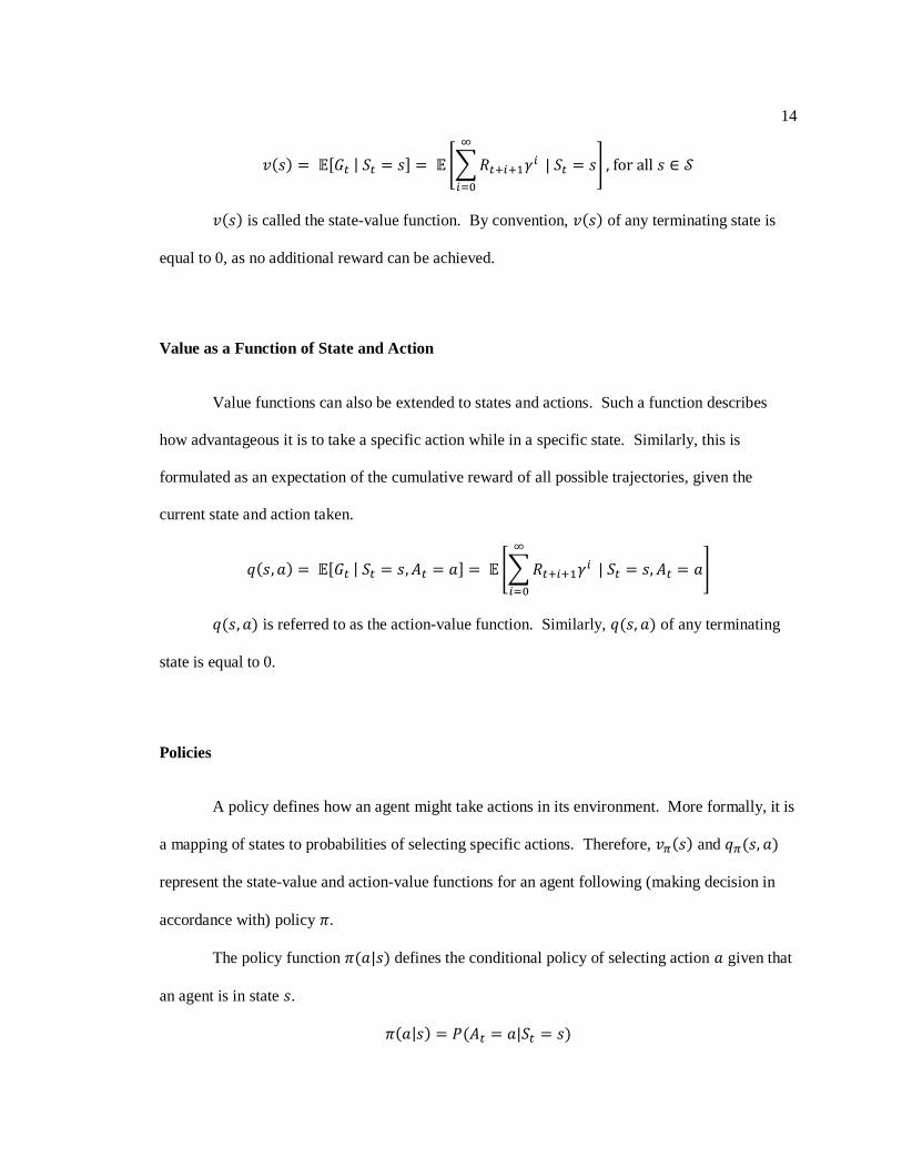
𝑣(𝑠) = 𝔼[𝐺𝑡 | 𝑆𝑡 = 𝑠] = 𝔼 [∑𝑅𝑡+𝑖+1𝛾𝑖

∞

𝑖=0

| 𝑆𝑡 = 𝑠] , for all 𝑠 ∈ 𝒮

𝑣(𝑠) is called the state-value function. By convention, 𝑣(𝑠) of any terminating state is

equal to 0, as no additional reward can be achieved.

Value as a Function of State and Action

Value functions can also be extended to states and actions. Such a function describes

how advantageous it is to take a specific action while in a specific state. Similarly, this is

formulated as an expectation of the cumulative reward of all possible trajectories, given the

current state and action taken.

𝑞(𝑠, 𝑎) = 𝔼[𝐺𝑡 | 𝑆𝑡 = 𝑠, 𝐴𝑡 = 𝑎] = 𝔼 [∑𝑅𝑡+𝑖+1𝛾𝑖

∞

𝑖=0

| 𝑆𝑡 = 𝑠, 𝐴𝑡 = 𝑎]

𝑞(𝑠, 𝑎) is referred to as the action-value function. Similarly, 𝑞(𝑠, 𝑎) of any terminating

state is equal to 0.

Policies

A policy defines how an agent might take actions in its environment. More formally, it is

a mapping of states to probabilities of selecting specific actions. Therefore, 𝑣𝜋(𝑠) and 𝑞𝜋(𝑠, 𝑎)

represent the state-value and action-value functions for an agent following (making decision in

accordance with) policy 𝜋.

The policy function 𝜋(𝑎|𝑠) defines the conditional policy of selecting action 𝑎 given that

an agent is in state 𝑠.

𝜋(𝑎|𝑠) = 𝑃(𝐴𝑡 = 𝑎|𝑆𝑡 = 𝑠)

15

The primary goal of a reinforcement learning algorithm is to learn an optimal policy

𝜋∗(𝑎|𝑠) that maximizes the expected cumulative reward. In determining this policy, the agent

can then proceed optimally at completing its task.

Bellman Equation

The Bellman equation is a fundamental property of Markov decision processes that

relates the value of a single state to the values of its successor states.

𝑣𝜋(𝑠) = ∑𝜋(𝑎|𝑠)

𝑎

∑ 𝑝(𝑠′, 𝑟 | 𝑠, 𝑎)

𝑠′,𝑟

[𝑟 + 𝛾𝑣𝜋(𝑠′)], for all 𝑠 ∈ 𝒮

Here, the recurrence relation relating the cumulative reward of a state to the cumulative

reward of its successor state is exploited. [16]

𝑣𝜋(𝑠) = 𝔼𝜋[𝐺𝑡|𝑆𝑡 = 𝑠]

= 𝔼𝜋[𝑅𝑡+1 + 𝛾𝐺𝑡+1|𝑆𝑡 = 𝑠]

= ∑ 𝜋(𝑎|𝑠)

𝑎

∑∑𝑝(𝑠′, 𝑟|𝑠, 𝑎)[𝑟 + 𝛾𝔼𝜋[𝐺𝑡+1|𝑆𝑡+1 = 𝑠′]]

𝑟𝑠′

= ∑ 𝜋(𝑎|𝑠)

𝑎

∑𝑝(𝑠′, 𝑟|𝑠, 𝑎)[𝑟 + 𝛾𝑣𝜋(𝑠′)]

𝑠′,𝑟

The Bellman equation uses the recurrence relation of cumulative reward to average over

all possible scenarios, weighted by its respective probability (under a policy) of occurring, to

determine the value of a state. More simply, the value of any given state is equal to the

discounted, expected value of the next state plus the reward received for transitioning to that

state.

16

Policy Optimality

A natural goal might be to seek an optimal policy, one which maximizes the cumulative

reward. But what makes one policy better than another?

A policy 𝜋1 is said to be better than another policy 𝜋2 if for all possible states, the value

function of 𝜋1 is greater than the value function of 𝜋2. That is, 𝜋1 ≥ 𝜋2 if and only if 𝑣𝜋1(𝑠) ≥

𝑣𝜋2, for all 𝑠 ∈ 𝒮. It naturally follows that the optimal policy must be better than all other

possible policies and as such, its value function must be greater in all states than the value

function of any other policy. Optimal policies are denoted by 𝜋∗. The corresponding state-value

function and action-value function of the policy are 𝑣∗(𝑠) and 𝑞∗(𝑠, 𝑎).

𝑣∗(𝑠) = max𝜋

𝑣𝜋(𝑠) for all 𝑠 ∈ 𝒮

𝑞∗(𝑠, 𝑎) = max𝜋

𝑞𝜋(𝑠, 𝑎) for all 𝑠 ∈ 𝒮, 𝑎 ∈ 𝒜

With complete knowledge, the optimal value function indicates which state (or state

action pairs) lead to the greatest cumulative reward. Some algorithms, for example, Q-Learning,

which will be discussed in Chapter 3, attempt to build a policy through direct approximation of

the optimal value functions.

Reward Functions

Given an understanding of value and policy, it is important to consider how immediate

reward may be assigned to the agent. Importantly, rewards should be assigned as to encourage

the agent to achieve an end goal, not to achieve intermediate goals. Rewards should define

exactly the goal of the agent, not the process one wishes the agent to take. For example,

assigning rewards to a Go playing agent to attain strategic formations may incite it to achieve

17

these positions at the expense of winning the game. Rather, reward should only be assigned for

winning the game.

In the case of episodic tasks, a large positive reward is often assigned only at the

conclusion of a successful episode (for example, winning a game), while a large negative reward

might be assigned at the conclusion of a failed episode (for example, losing a game).

Another common addition to the reward function is to assign very small negative reward

for every timestep that a goal is not achieved. In doing so, an agent may learn to complete a task

as quickly as possible.

18

Chapter 3

Algorithms

Often, reinforcement learning algorithms seek to find or estimate an optimal policy, one

which selects actions that best maximize cumulative future reward at each state in which the

agent finds itself. Other algorithms may seek to explore the environment in the absence of the

reward signal, for example to induce a distribution of state space visitation that is as uniform as

possible [22]. However, when the goal is to accomplish the task defined by the reward signal, the

goal is to learn an optimal policy.

Exploitation-Exploration Tradeoff

There exists an inherent tradeoff between a reinforcement agent exploiting its current

policy to accumulate reward and exploring its environment to learn about other, possible greater

rewards. On one hand, the agent must exploit the best actions in order to achieve reward.

However, to learn which actions are the best, it must explore, deviating from known optimal

actions in search of unknown, better actions. This phenomenon is known as the exploitation-

exploration tradeoff.

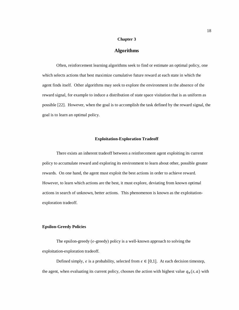
Epsilon-Greedy Policies

The epsilon-greedy (𝜖-greedy) policy is a well-known approach to solving the

exploitation-exploration tradeoff.

Defined simply, 𝜖 is a probability, selected from 𝜖 ∈ [0,1]. At each decision timestep,

the agent, when evaluating its current policy, chooses the action with highest value 𝑞𝜋(𝑠, 𝑎) with

19

probability 1 − 𝜖. It chooses a random action from the set of valid actions with probability 𝜖. In

doing so, the agent is forced to explore potentially unseen situations, even against what the policy

recommends.

Epsilon is often decayed throughout the learning process. High values enable more

learning and exploration, at the expense of achieving a high reward. After many episodes of

learning, epsilon decays, enabling the agent to tune its current policy in an attempt to achieve

optimal behavior.

Other algorithms exist to solve the exploitation-exploration tradeoff such as upper

confidence bounding and Thompson sampling [23], [24].

Algorithm Characteristics

Model and Model-Free Algorithms

Model-based algorithms are algorithms that use some known model of the environment

to aid in decision making. However, since models must be quite accurate to be leveraged

usefully, other, model-free approaches are often preferable when an explicit model of the

environment is unknown.

Model-free agents, on the other hand, require no knowledge at all of the environment.

They can be thought of as pure trial-and-error learners, learning the meaning of states and the

value of actions taken in those states without necessarily being able to reason how the

environment might change in response to an action it takes.

20

On-Policy and Off-Policy Algorithms

In the process of learning, a reinforcement learning agent’s goal is to generate a policy

that, when followed, best achieves a maximum cumulative reward. One way to do this is via an

on-policy algorithm, whereby an agent chooses an action from a policy, experiences some reward

and new state, and then updates the policy by which it made the decision.

Conversely, off-policy algorithms describe a class of algorithms whereby the policy

being improved is not the same policy by which decisions are being made in the learning process.

Often, off-policy algorithms attempt to directly build the optimal policy while being controlled by

another policy.

Dynamic Programming, Monte-Carlo, and Temporal Differencing Algorithms

Dynamic programming, Monte-Carlo, and temporal differencing algorithms are three

major classes of algorithms for developing policies under reinforcement learning.

Dynamic programming techniques closely follow the theory introduced by the recursive

Bellman equation. Through the use of the value function, repeated policy evaluation and

improvement steps update the current policy being examined. Convergence occurs when updates

become zero and the Bellman equation is satisfied. The major drawback of pure dynamic

programming techniques for reinforcement learning is that a perfect model of the MDP

representing the environment is needed. Additionally, the computational complexity of DP

methods is immense. Both of these constraints are very often infeasible in real-world

applications of RL.

Monte-Carlo approaches differ from dynamic programming in that they do not require a

perfect model of the environment; rather they learn from experiences: samples of state, action,

21

reward, state tuples experienced by the agent in the environment. Monto-Carlo methods consider

complete runs of the agent under a policy, from its initial state to a terminating state, and average

the return experienced from starting in that initial state to estimate the value of that initial state.

However, managing sufficient exploration to achieve an optimal policy is more difficult for

Monte-Carlo methods.

Temporal differencing algorithms combine aspects of both dynamic programming and

Monte-Carlo approaches for solving the reinforcement learning problem. Temporal differencing

methods do not require a complete knowledge of the environment, but rather learn from

experiences, similar to Monte-Carlo methods. Additionally, they bootstap by updating estimates

for the value functions using other estimates. Unlike Monte-Carlo methods, TD algorithms do

not require full samples of episodes, experiences from the initial state to a terminating state,

rather they make updates at each transition of the MDP. Making use of the recursive relationship

between cumulative rewards at each step, the value function for a state is updated through a

weighted differencing of the current state’s value function and that of the next state. The simplest

temporal differencing update rule, is:

𝑉(𝑆𝑡) ← 𝑉(𝑆𝑡) + 𝛼[𝑅𝑡+1 + 𝛾𝑉(𝑆𝑡+1) − 𝑉(𝑆𝑡)]

Temporal differencing is a key component of one of the most famous reinforcement

learning algorithms, Q-Learning.

Q-Learning

One of the most well-known breakthroughs in reinforcement learning was the

introduction of Q-Learning by Christopher Watkins [25], [26].

Q-Learning is a model-free algorithm: it learns directly from experience without needing

an explicit model of the environment. It is also an off-policy algorithm: it directly approximates

22

the optimal value function, without evaluating a specific policy. Finally, Q-Learning is

considered a temporal-difference algorithm: it updates estimates of the value function by

bootstrapping from other learned estimates.

Q-Learning works by learning an approximate action-value function, 𝑄(𝑆𝑡 , 𝐴𝑡) from

experience. As Q-Learning is an off-policy algorithm, it directly approximates 𝑞∗(𝑠, 𝑎), the

optimal action-value function, and, being off-policy, its approximations are independent of the

policy being followed.

Watkins defines the Q-Learning update rule as:

𝑄(𝑆𝑡 , 𝐴𝑡) ← 𝑄(𝑆𝑡 , 𝐴𝑡) + 𝛼 [𝑅𝑡+1 + 𝛾 max𝑎

𝑄(𝑆𝑡+1, 𝑎) − 𝑄(𝑆𝑡 , 𝐴𝑡)]

where 𝛼 is the learning rate selected from 𝛼 ∈ (0,1]. At each step it updates the current

estimation of 𝑄(𝑆𝑡 , 𝐴𝑡) based on the reward it receives and the other estimates for 𝑄(𝑆𝑡+1, 𝐴𝑡+1).

Since Q-Learning directly builds the optimal state-action value function, the corresponding

optimal policy is one that selects the next action with highest value.

𝜋∗(𝑠|𝑎) = 1, 𝑎 ∈ argmax𝑎′

𝑞∗(𝑠, 𝑎′)

In its basic form, Q-Learning is a tabular approach. It records in a table the values of

𝑄(𝑆𝑡 , 𝐴𝑡) for which it has experienced, initializes for first-seen occurrences, and updates the

table. Pseudocode for basic Q-Learning with epsilon-greedy exploration is described in Figure 3-

1.

23

Convergence Guarantees

The action-value function developed by Q-Learning, for situations modelled by finite

Markov decision processes, converges to the true optimal state-action value function with

probability 1, when all state-action pairs are visited infinitely many times [27]. In practice, the Q-

Learning algorithm is run until approximate convergence is observed.

Issues with Tabular Q-Learning

One of the major issues of deploying tabular Q-Learning is with memory. The algorithm

requires tabular storage of action (q) values for all possible pairs of state and actions. For systems

with many states and actions, these memory requirements often scale out of the bounds of modern

storage limits. Additionally, with a growing number of state-action pairs, visitation of each state-

Q Learning

Initialize discount factor 𝛾 ∈ [0,1], step size 𝛼 ∈ (0,1], exploration rate 𝜖 ∈ (0,1)

Initialize 𝑄(𝑠, 𝑎) = 0, for all 𝑠 ∈ 𝒮, 𝑎 ∈ 𝒜 (or arbitrarily, except for terminal states)

Loop for Each Episode

Initialize initial state S

Loop for Each Step in Episode

Choose the optimal action 𝐴 = argmax𝑎′

𝑄(𝑆, 𝑎′) with probability 1 − 𝜖

Choose a random action 𝐴 ∈ 𝒜(𝑆) with probability 𝜖

Take action 𝐴 and observe the resultant reward 𝑅 and next state 𝑆′

Update table 𝑄(𝑆, 𝐴) ← 𝑄(𝑆, 𝐴) + 𝛼[𝑅 + 𝛾 max𝑎′

𝑄(𝑆′, 𝑎′) − 𝑄(𝑆, 𝐴)]

Update state 𝑆 ← 𝑆′

End When S is a Terminal State

End After N Episodes

Figure 3-1: Epsilon Greedy Q-Learning Pseudocode

24

action pair becomes infeasible. Additionally, Q-Learning is incapable of generalizing between

any notion of “similar” states. Tabular lookup prohibits this generalization.

Deep Q-Learning

Advances in deep learning, the process of using many-layered neural networks, enabled

the emergence of Deep Q-Learning. Deep Q-Learning is an approach that leverages the benefits

of both Q-Learning and deep neural networks as state-action value function approximators. Deep

Q-Learning replaces the tabular lookup of Q-Learning with a neural network function

approximator. The pseudocode for a basic Deep Q-Learning with epsilon greedy exploration is

depicted in Figure 3-2.

The use of an accurate function approximator overcomes the issue of memory scalability

induced by traditional Q-Learning. The memory requirements are no longer scaled with the

Deep Q Learning


Initialize 𝑄 neural network with random weights








Set 𝑌 = {𝑅

𝑅 + 𝛾 max𝑎′

𝑄(𝑆′, 𝑎′) for terminal 𝑆′

for non-terminal 𝑆′

Perform gradient descent on (𝑌 − 𝑄(𝑆, 𝐴))2




Figure 3-2: Epsilon Greedy Deep Q-Learning Pseudocode

25

number of possible state-action pairs, but rather with the static number of weights of the chosen

Q-Network, which is often much less than the tabular representation. However, since the neural

network is a function approximator, formal convergence guarantees of Q-Learning are no longer

provable.

Additionally, the Q-Network enables, to an extent, generalization of experiences. While

Q-Learning’s tabular storage meant similar state-action pairs would be seen as completely

separate events, Deep Q-Learning allows for generalization between them, correlating the two

samples to a potentially similar q-value.

Catastrophic Forgetting

One major drawback and potential issue with the use of a neural network for state-action

value approximation is the phenomenon of catastrophic forgetting. Catastrophic forgetting is the

process by which a neural network trained to complete a specific task is re-trained to complete a

new task, losing the weight information needed to successfully complete the original task,

essentially ‘forgetting’ this original task [28].

Given the breadth of potential actions and strategies a reinforcement learning agent might

employ, learned, desired behavior may be overwritten by future experiences, especially when the

desired behavior is not frequently reinforced/trained.

Experience Replay

The idea of experience replay was introduced by Google DeepMind in their pursuit to

master Atari games with reinforcement learning [3]. Experience replay is the process of storing

an agent’s experiences (state, action, reward, state tuples) in a dataset. Then, instead of updating

26

the Q-Learning rule immediately after a transition, a batch of many, random, past transitions is

sampled and used to update the Deep Q-Learning network.

The pseudocode for a basic Deep Q-Learning algorithm with experience replay and

epsilon greedy exploration is depicted in Figure 3-3.

Experience replay provides many benefits to Deep Q-Learning. Firstly, it enables re-use

of data. Sampling transitions potentially many times and using for training makes the collected

experiences more efficient, as the experiences are used more than once. Additionally, the random

sampling reduces the variance of updates made to the Q-Network. Since the batch of updates

likely will not all come from the same trajectory, strong correlations between subsequent

transitions are broken and do not bias the network when training. Finally, when training greedily

on-policy, experience replay helps break unwanted feedback loops of reinforcing behavior, and,

Deep Q Learning with Experience Replay


Initialize 𝑄 neural network with random weights

Initialize experience memory 𝒟 to capacity 𝑀 tuples








Store transition (𝑆, 𝐴, 𝑅, 𝑆′) in 𝒟

Randomly sample a transition (𝑠, 𝑎, 𝑟, 𝑠′) (or batch of transitions) from 𝒟

Set y= {𝑟

𝑟 + 𝛾 max𝑎′

𝑄(𝑠′, 𝑎′) for terminal 𝑠′

for non-terminal 𝑠′

Perform gradient descent on (𝑦 − 𝑄(𝑠, 𝑎))2




Figure 3-3: Epsilon Greedy Deep Q-Learning with Experience Replay Pseudocode

27

sampling past experiences, reduces the likelihood of catastrophic forgetting, helping to smooth

the learning process and avoid local minima [3].

28

Chapter 4

Problem and Approach

The goal of this thesis was to see if reinforcement leaning techniques could be applied, in

simulation, the problem of autonomous, unmanned, underwater vehicle (AUV, or UUV)

navigation and contact avoidance. The autonomous navigation of a UUV is a unique task in that

such vehicles experience many hardware limitations and lack explicit knowledge of their

environment.

Unmanned Underwater Vehicles (UUVs)

Unmanned underwater vehicles are being used for various maritime missions with an

objective to be unobtrusive. For the sake of this theses, the exact nature of the UUV’s mission

will be unspecified. The goal will be to successfully navigate the vehicle to the site of a mission

without discovery or interference with unknown objects.

Figure 4-1: An Unmanned Underwater Vehicle (UUV) [29]

29

Limitations of a UUV

Primary limitations of unmanned underwater vehicles arise both from their small profile

and need to remain undetected. In constructing a UUV it is often preferred or necessary to forgo

expensive, large, or complex equipment.

Active sonar (SOund Navigation And Ranging) is a common technique that enables

maritime agents to sense their environment. Pulses of sound are emitted through the water and

will reflect off of sufficiently large and geometric objects. Given the time between emission and

receipt of a reflected sound wave, the existence and approximate distance to an (even unknown)

object can be computed [30].

Passive sonar is a similar technique but lacks active emission of sound waves. Instead,

arrays of hydrophones only listen for sound waves emitted from other sources. Using the array,

the bearing (angle) to the source of the sound emission can be computed. Sufficiently large or

complex passive sonar systems may also be able to estimate the distance to the source of the

sound via triangulation [30].

In general, UUVs are unable to make use of active sonar techniques. This is dually due

to both in part of their inability to tow the larger equipment and their desire to remain covert by

not emitting explicit sound waves. Use of active sonar systems on a UUV would certainly risk its

detection. As a result, we assume a UUV to have knowledge of the bearing to both known and

unknown contacts (other underwater vehicles, ships, obstructions, etc.) but have no knowledge of

the distance to such objects.

A secondary limitation of UUVs are their general inability to receive signals from above

the water when significantly submerged. Sufficiently low frequency radio can often be broadcast

and received to vehicles significantly submersed, however such equipment is normally not carried

by a UUV. One issue that arises from lack of communication with the surface is that of control.

30

Manually controlled vehicles are infeasible without consistent communication between the UUV

and a remote operator. This thesis seeks to explore this issue through autonomous navigation.

Another issue that arises is that of global positioning. GPS signals cannot reach the UUV if

submerged. However, this issue is often resolved through periodic surfacing and accurate inertial

units which enable an approximate global position to be computed in between surfacing.

Assumptions of the Simulated UUV

We assume a very limited model of a UUV in simulation.

In terms of control, we assume the UUV to navigate below the surface constrained to a

two-dimensional plane. It operates only via forward motion and rotation. The UUV may

increase or decrease its rotational speed in discrete increments. If increasing its speed above the

maximum threshold, such an increase has no affect. Similarly, decreasing its speed below zero

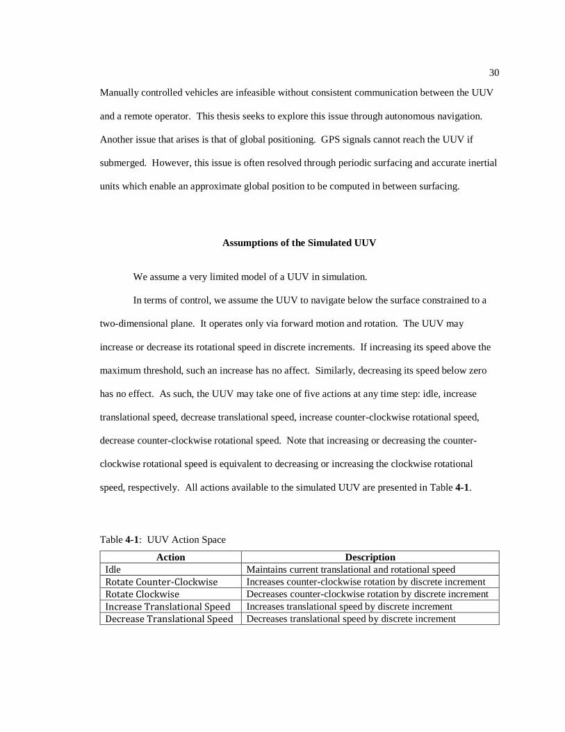
has no effect. As such, the UUV may take one of five actions at any time step: idle, increase

translational speed, decrease translational speed, increase counter-clockwise rotational speed,

decrease counter-clockwise rotational speed. Note that increasing or decreasing the counter-

clockwise rotational speed is equivalent to decreasing or increasing the clockwise rotational

speed, respectively. All actions available to the simulated UUV are presented in Table 4-1.

Table 4-1: UUV Action Space

Action Description

Idle Maintains current translational and rotational speed

Rotate Counter-Clockwise Increases counter-clockwise rotation by discrete increment

Rotate Clockwise Decreases counter-clockwise rotation by discrete increment

Increase Translational Speed Increases translational speed by discrete increment

Decrease Translational Speed Decreases translational speed by discrete increment

31

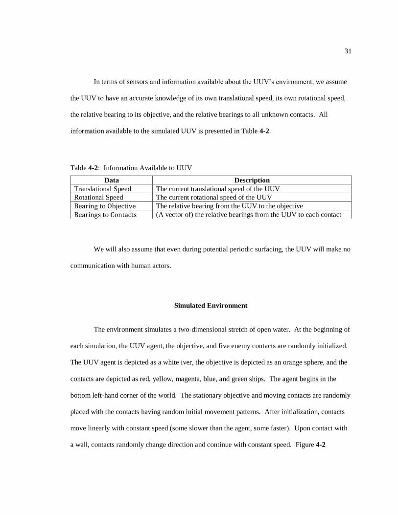
In terms of sensors and information available about the UUV’s environment, we assume

the UUV to have an accurate knowledge of its own translational speed, its own rotational speed,

the relative bearing to its objective, and the relative bearings to all unknown contacts. All

information available to the simulated UUV is presented in Table 4-2.

We will also assume that even during potential periodic surfacing, the UUV will make no

communication with human actors.

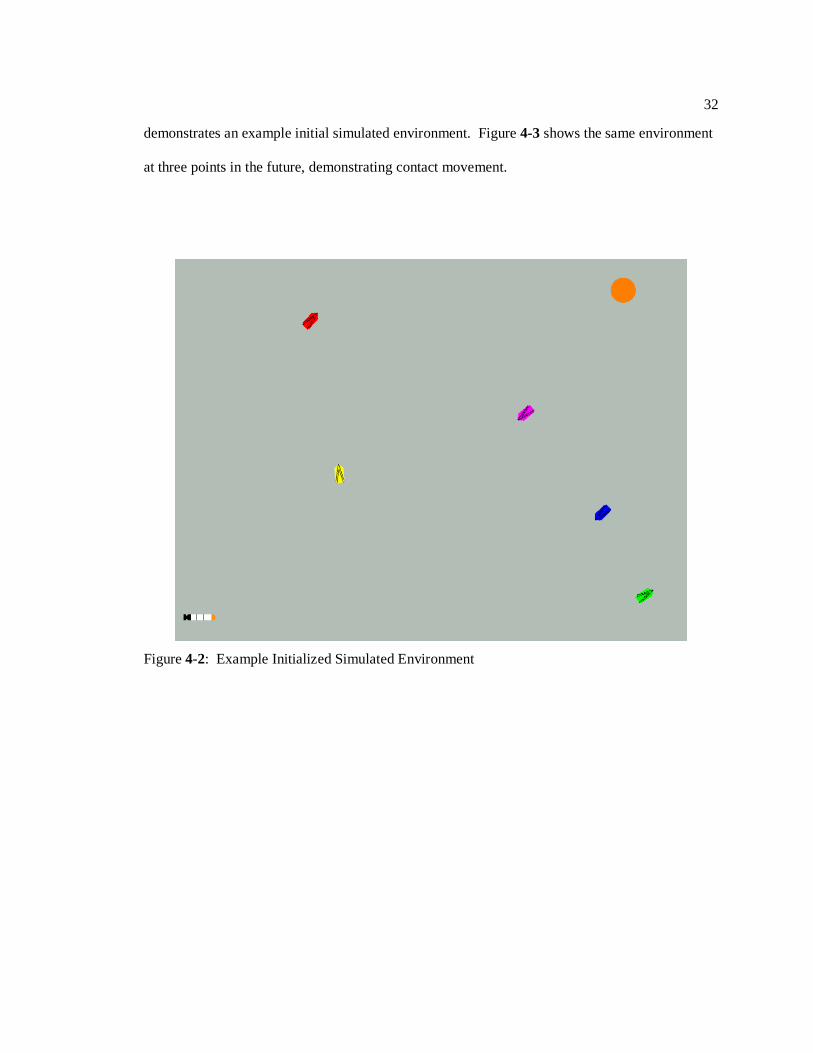
Simulated Environment

The environment simulates a two-dimensional stretch of open water. At the beginning of

each simulation, the UUV agent, the objective, and five enemy contacts are randomly initialized.

The UUV agent is depicted as a white iver, the objective is depicted as an orange sphere, and the

contacts are depicted as red, yellow, magenta, blue, and green ships. The agent begins in the

bottom left-hand corner of the world. The stationary objective and moving contacts are randomly

placed with the contacts having random initial movement patterns. After initialization, contacts

move linearly with constant speed (some slower than the agent, some faster). Upon contact with

a wall, contacts randomly change direction and continue with constant speed. Figure 4-2

Table 4-2: Information Available to UUV

Data Description

Translational Speed The current translational speed of the UUV

Rotational Speed The current rotational speed of the UUV

Bearing to Objective The relative bearing from the UUV to the objective

Bearings to Contacts (A vector of) the relative bearings from the UUV to each contact

32

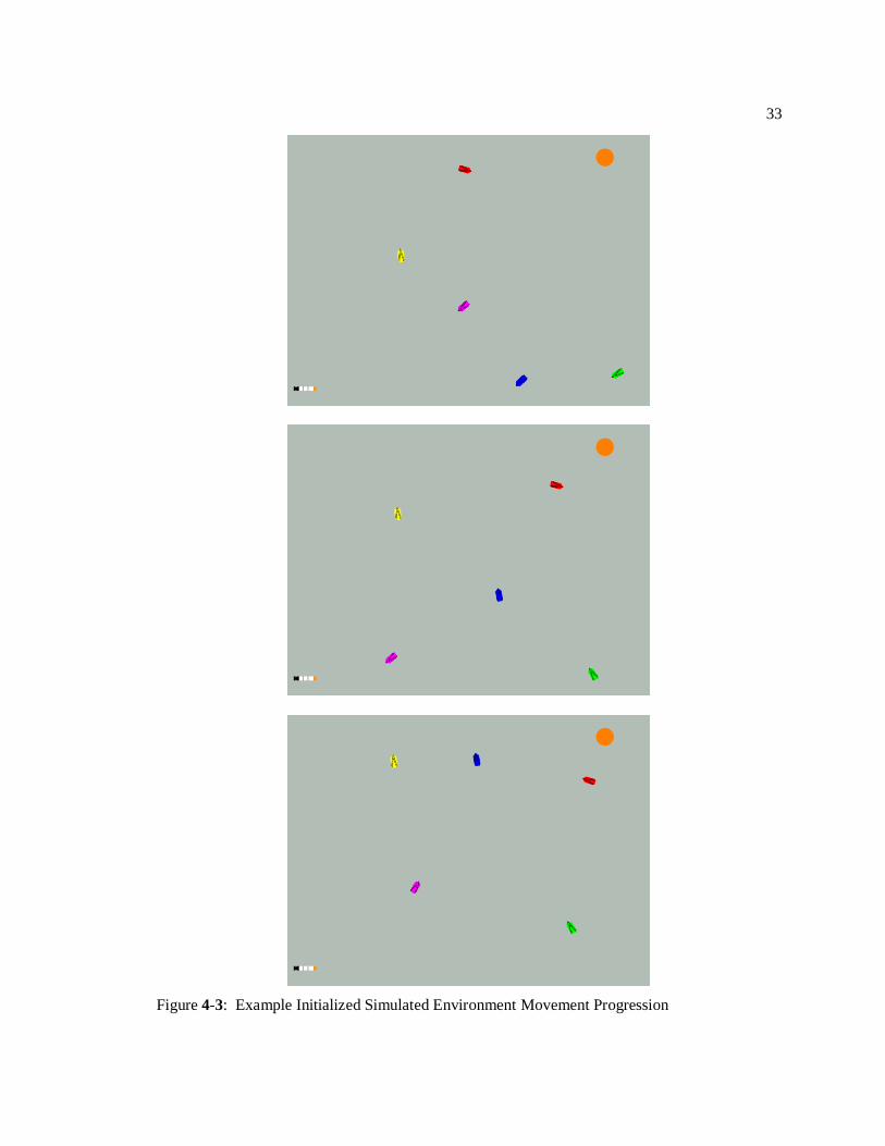
demonstrates an example initial simulated environment. Figure 4-3 shows the same environment

at three points in the future, demonstrating contact movement.

Figure 4-2: Example Initialized Simulated Environment

33

Figure 4-3: Example Initialized Simulated Environment Movement Progression

34

Additional Parameters

Additional parameters that may be varied in the simulated environment include the radius

of the objective and the contacts. A larger objective radius corresponds with a less precise

approach required of the agent to succeed in its mission. A larger contact radius corresponds with

a greater area of detection and increased chance of failing the mission. In reality, a larger contact

radius would correspond with the contact’s increased ability to detect the UUV agent. The

objective radius was 25 units for all experiments.

Figure 4-4: Contacts with Hitboxes (25, 50, and 100 units)

35

State Representation

At the beginning of each timestep, the UUV accesses the information of its environment

(reads its sensors). This information includes just the current speeds of the UUV and the bearings

to all objects. This vector of information is summarized in Figure 4-5.

To encapsulate history information, the UUV records and remembers the past four

instantaneous state vectors with configurable sampling rate. The sampling rate is equivalent to

the decision-making rate. That is, for every timestep that the agent is able to take an action, it

also samples the instantaneous state. This aggregate 1x32 vector is passed to the reinforcement

learning algorithm.

Reward Architecture

The reward function varies among experiments, as will be discussed in Chapter 5. In

general, at every decision-making interval, the agent receives a positive reward if it has reached

the objective, a negative reward if it has collided with (been discovered by) a contact, and a small

negative reward for timesteps where neither occur. The small negative penalty is much smaller

instantaneous state =

[ 𝑎𝑔𝑒𝑛𝑡 𝑡𝑟𝑎𝑛𝑠𝑙𝑎𝑡𝑖𝑜𝑛𝑎𝑙 𝑠𝑝𝑒𝑒𝑑𝑎𝑔𝑒𝑛𝑡 𝑟𝑜𝑡𝑎𝑡𝑖𝑜𝑛𝑎𝑙 𝑠𝑝𝑒𝑒𝑑𝑏𝑒𝑎𝑟𝑖𝑛𝑔 𝑡𝑜 𝑜𝑏𝑗𝑒𝑐𝑡𝑖𝑣𝑒

𝑏𝑒𝑎𝑟𝑖𝑛𝑔 𝑡𝑜 𝑐𝑜𝑛𝑡𝑎𝑐𝑡 1𝑏𝑒𝑎𝑟𝑖𝑛𝑔 𝑡𝑜 𝑐𝑜𝑛𝑡𝑎𝑐𝑡 2𝑏𝑒𝑎𝑟𝑖𝑛𝑔 𝑡𝑜 𝑐𝑜𝑛𝑡𝑎𝑐𝑡 3𝑏𝑒𝑎𝑟𝑖𝑛𝑔 𝑡𝑜 𝑐𝑜𝑛𝑡𝑎𝑐𝑡 4𝑏𝑒𝑎𝑟𝑖𝑛𝑔 𝑡𝑜 𝑐𝑜𝑛𝑡𝑎𝑐𝑡 5 ]

Figure 4-5: Instantaneous State Vector

36

(less than 1% the magnitude) of either success and failure reward or penalty. An episode

terminates upon receipt of a successful or failed mission.

37

Chapter 5

Implementation and Evaluation

The simulator described in Chapter 4 was implemented in Python, using the Arcade

library for visuals and the Keras and TensorFlow libraries for neural networks. All reinforcement

learning modules were custom developed for this thesis.

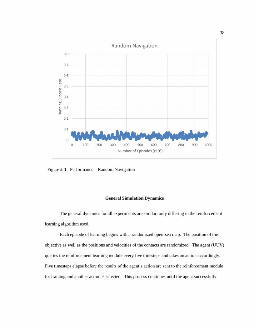
Baseline – Random Walk

The detection radius for contacts was set to 25 units. Allowing the UUV to randomly

navigate until successfully arriving at the objective or until detection forms the baseline for future

experiments. Performance is measured as a running average success rate over the past 100 trials.

As seen in Figure 5-1, the random-walk UUV is almost never successful. The average success

rate was 3.60%; these were likely instances where the objective was randomly generated in very

close proximity to the agent.

38

General Simulation Dynamics

The general dynamics for all experiments are similar, only differing in the reinforcement

learning algorithm used..

Each episode of learning begins with a randomized open-sea map. The position of the

objective as well as the positions and velocities of the contacts are randomized. The agent (UUV)

queries the reinforcement learning module every five timesteps and takes an action accordingly.

Five timesteps elapse before the results of the agent’s action are sent to the reinforcement module

for training and another action is selected. This process continues until the agent successfully

Figure 5-1: Performance – Random Navigation

0

0.1

0.2

0.3

0.4

0.5

0.6

0.7

0.8

0 100 200 300 400 500 600 700 800 900 1000

Ru

nn

ing

Succ

ess

Rat

e

Number of Episodes (x101)

Random Navigation

39

reaches the objective or until it is detected by one of the moving contacts. The time from

initialization until attainment of success or failure is considered one episode.

Tabular Q-Learning

As discussed in Chapter 3, tabular Q-Learning is infeasible for this problem, as the

immensely large state space would be impossible to visit, and the resulting q-values would be

impossible to physically store without significant hardware and time overhead.

Deep Q-Learning

A Deep Q-Learning module was implemented as described in Chapter 4.

At every decision-making interval, the agent sends information about its previous state,

the action it took, the reward it received from taking that action, and the new state at which it

arrived from taking that action. For the Deep Q-Learning implementation, the reinforcement

learning module computes the target value as:

target = {𝑅

𝑅 + 𝛾 max𝑎′

𝑄(𝑆′, 𝑎′) for terminal 𝑆′

for non-terminal 𝑆′

The maximum q (action) value is computed from the resultant state using the current q-

network. The module then backpropagates this target value through the neural network to update

the weights corresponding with this situation.

40

Network Architecture

A neural network was designed using Keras and Tensorflow to serve as a function

approximator for the q (action-value) function. The input layer of the network is 32 units,

representing the previous four timesteps for each of the eight features. The output layer of the

network is 5 units, representing the q-value for each of the five possible actions.

The following experiment uses two dense hidden layers of 20 and 50 neurons,

respectively. For training, the loss function used was mean squared error. All layers used a

hyperbolic tangent activation function, except for the output layer, which used a linear activation

function.

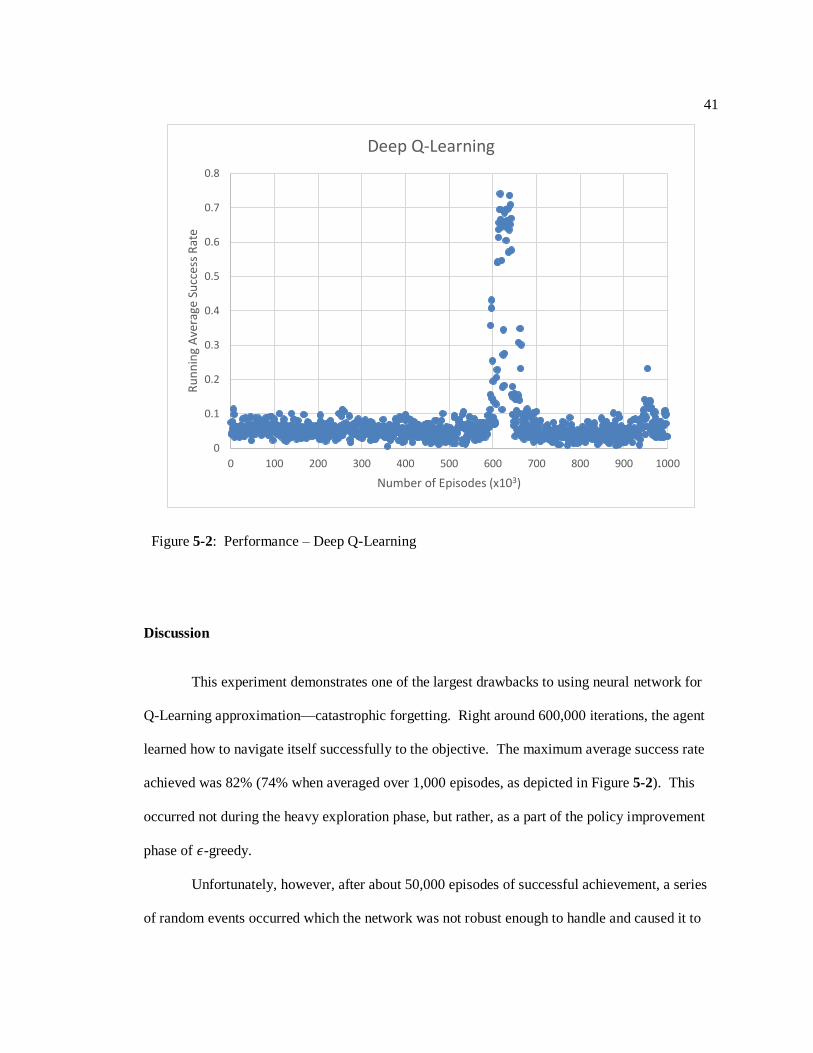
Performance

This procedure was run for 1,000,000 episodes with a contact radius of 10 units. The

exploration rate 𝜖 began at 1.0 and decayed linearly for the first 50% of episodes to 0.1 and

remained at 0.1 for the remaining episodes. Figure 5-2 shows the running average performance

(success rate) for the procedure. Training took 277,630.950 seconds (approximately 3 days).

41

Discussion

This experiment demonstrates one of the largest drawbacks to using neural network for

Q-Learning approximation—catastrophic forgetting. Right around 600,000 iterations, the agent

learned how to navigate itself successfully to the objective. The maximum average success rate

achieved was 82% (74% when averaged over 1,000 episodes, as depicted in Figure 5-2). This

occurred not during the heavy exploration phase, but rather, as a part of the policy improvement

phase of 𝜖-greedy.

Unfortunately, however, after about 50,000 episodes of successful achievement, a series

of random events occurred which the network was not robust enough to handle and caused it to

Figure 5-2: Performance – Deep Q-Learning

0

0.1

0.2

0.3

0.4

0.5

0.6

0.7

0.8

0 100 200 300 400 500 600 700 800 900 1000

Ru

nn

ing

Ave

rage

Su

cces

s R

ate


Deep Q-Learning

42

diverge. In the remaining training time, the network was not able to recover. Catastrophic

forgetting is a property of learning sequential tasks using neural networks. The process of the

agent’s navigation is inherently sequential as it depends on temporal input data. By

backpropagating potentially non-representative sequences of events sequentially through the

network, the weights that enabled the q-network to complete the task were overwritten.

Implementing experience replay memory is one way to combat catastrophic forgetting in

reinforcement learning problems.

Deep Q-Learning with Experience Replay

The Deep Q-Learning module above was augmented with experience replay memory. At

every decision-making interval, the simulator still sends information about its previous state, the

action it took, the reward it received from taking that action, and the new state it arrived at from

taking that action. Instead of immediately backpropagating the updated target, it stores the state,

action, reward, state tuple in a 1,000,000 entry FIFO cache.

Next, every 1,000 transitions, it randomly samples a batch of 2,000 transitions from this

memory, computes the appropriate target values according to the update rule, and backpropagates

the entire batch through the network.


A similar neural network was designed to serve as a function approximator for the q

(state-action value) function. The input layer of the network is 32 units, representing the previous

four timesteps for each of the eight features. The output layer of the network is 5 units,

representing the q-value for each of the five possible actions.

43

The following experiment uses two dense hidden layers of 32 and 64 neurons,

respectively. For training, the loss function used was mean squared error. All layers used a

hyperbolic tangent activation function, except for the output layer, which used a linear activation

function.

Performance

This procedure was run for 1,000,000 episodes with a contact radius of 25 units. The

exploration rate 𝜖 began at 1.0 and decayed linearly for the first 50% of episodes to 0.1 and

remained at 0.1 for the remaining episodes. Figure 5-3 shows the running average performance

(success rate) for the procedure. Training took 71,801.199 seconds (approximately 20 hours).

44

Discussion

This experiment converged quite cleanly to a running average success rate of 70%. The

maximum running average success rate achieved was 87%. As Figure 5-3 depicts, the

convergence occurred right around 500,000 episodes, when the exploration rate 𝜖 completely

tapered to 0.1. This indicates that the same results likely would have been achieved with even

fewer training episodes.

It appears that the replay memory broke the correlations between successive transitions

and enabled the agent to learn without forgetting. This technique avoids making many similar-

Figure 5-3: Performance – Deep Q-Learning with Experience Replay

0

0.1

0.2

0.3

0.4

0.5

0.6

0.7

0.8

0 100 200 300 400 500 600 700 800 900 1000

Ru

nn

ing

Succ

ess

Rat

e


Deep Q-Learning with Experience Replay

45

valued updates to the neural network. Another benefit of this implementation was the shorter

running time, while also training on much more data due to the data re-use principle of

experience replay. The trained UUV does a good job, although not perfect, of avoiding collisions

with the contacts.

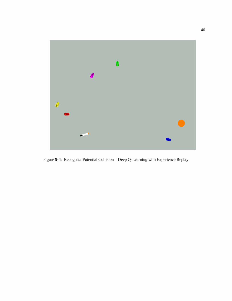
Example Behavior

This implementation has induced the agent to learn some interesting behavior. To some

extent, the agent is able to recognize when it is on path for a collision. When this occurs, the

UUV recognizes the scenario, performs a trajectory correction maneuver, and continues linearly

to the objective, avoiding the collision, and successfully reaching the objective. Figures 5-4, 5-5

and 5-6 depict one of these scenarios, where the UUV avoids a collision with the blue contact. In

Figure 5-4, the UUV recognizes it is on path to collide with the blue contact. In Figure 5-5, it

performs a maneuver to change its trajectory. In Figure 5-6, it continues on course to the

objective.

46

Figure 5-4: Recognize Potential Collision – Deep Q-Learning with Experience Replay

47

Figure 5-5: Perform Trajectory Correction – Deep Q-Learning with Experience Replay

48

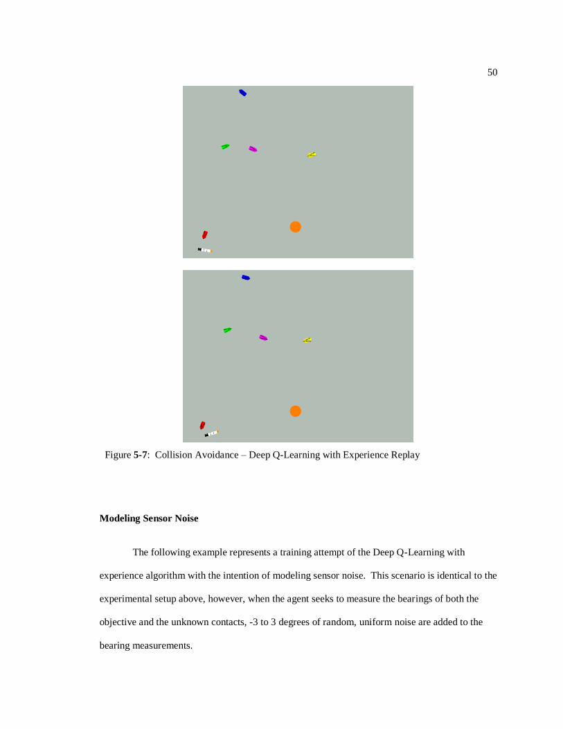
Figure 5-7 depicts another situation, where right from the initialization, the UUV is faced

with a potential collision with the red contact. Right from the beginning, it performs a maneuver

to avoid being detected by the quickly moving red contact.

Figure 5-6: Continue on Course – Deep Q-Learning with Experience Replay

49

50

Modeling Sensor Noise

The following example represents a training attempt of the Deep Q-Learning with

experience algorithm with the intention of modeling sensor noise. This scenario is identical to the

experimental setup above, however, when the agent seeks to measure the bearings of both the

objective and the unknown contacts, -3 to 3 degrees of random, uniform noise are added to the

bearing measurements.

Figure 5-7: Collision Avoidance – Deep Q-Learning with Experience Replay

51

As shown in Figure 5-8, the algorithm is robust enough to handle this uncertainty,

although there is a non-trivial drop in performance. The running average success rate is about

58% after convergence.

Deep Q Learning with Experience Replay and Reward Shaping

The Deep Q Learning with Experience Replay module above (without noise) was

augmented with shaped (annealed) rewards to encourage contact avoidance. At every decision-

making interval, the simulator still sends information about its previous state, the action it took,

the reward it received from taking that action, and the new state it arrived at from taking that

Figure 5-8: Performance – Deep Q-Learning with Experience Replay with Sensor Noise

0

0.1

0.2

0.3

0.4

0.5

0.6

0.7

0.8

0 100 200 300 400 500 600 700 800 900 1000

Ru

nn

ing

Succ

ess

Rat

e


Modelling Sensor Noise

52

action. Again, these transitions were stored in a 1,000,000 entry FIFO cache, and every 1,000

transitions, 2,000 transitions were randomly sampled, and backpropagated accordingly.

However, the reward function was shaped over time for this experiment. The penalty

was increased slowly over time to still encourage navigation behavior, while simultaneously

encouraging the UUV to better avoid contacts. The reward shaping schedule can be seen in Table

5-1. This process was run for 1,200,000 episodes.


The same neural network architecture as used for Deep Q-Learning with Experience

Replay was used for the reward shaping implementation. The input layer of the network is 32

units, representing the previous four timesteps for each of the eight features. The output layer of

the network is 5 units, representing the q-value for each of the five possible actions. Two hidden

layers of 32 and 64 neurons, respectively were within. For training, the loss function used was

mean squared error. All layers used a hyperbolic tangent activation function, except for the

output layer, which used a linear activation function.

Table 5-1: Reward Shaping Schedule

Episode Range Penalty for Detection

0 to 499,999 -100.0

500,000 to 749,999 -100.0 to -500.0 (linear decay)

750,000 to 999,999 -500.0 to -1,200.0 (linear decay)

1,000,000 to 1,200,000 -1,200.0

53

Performance

This procedure was run for 1,200,000 episodes. The exploration rate 𝜖 began at 1.0 and

decayed linearly for the first 50% of episodes to 0.1 and remained at 0.1 for the remaining

episodes. Figure 5-9 shows the running average performance (success rate) for the procedure.

Training took 264,816.805 seconds (approximately 3 days).

Figure 5-9: Performance – Deep Q-Learning with Experience Replay and Reward Shaping

0

0.1

0.2

0.3

0.4

0.5

0.6

0.7

0.8

0 100 200 300 400 500 600 700 800 900 1000

Ru

nn

ing

Succ

ess

Rat

e

Number of Episodes (x1.2⋅103)

Deep Q-Learning with Experience Replay and Reward Shaping

54

Discussion

This experiment finished with a running average success rate of 57%. The maximum

running average success rate achieved was 82%. As Figure 5-9 depicts, the experiment

converges to a success rate of approximately 65% reasonably before the end of the exploration

phase at 600,000 episodes. After that, during the annealing phase, performance degrades slightly,

with a small increase in the variance of success rate. Although the rate of successful navigation

to the objective decreases slightly, it does appear that the agent has learned an increased ability to

avoid contacts in some situations.

Example Behavior

In one run, the agent persisted for a total of 118 timesteps and successfully reached the

objective, while also successfully avoiding several close encounters with fast-moving contacts.

More specifically, three behaviors were observed which demonstrate the agent’s understanding of

its complex and dynamic environment.

The agent appears to have learned the ability to stop its course to both avoid a collision

and to adjust its course. Stopping had previously been unseen, as the agent preferred to proceed

always at maximum speed, as encouraged by the timestep penalty. Such a maneuver is depicted

in Figure 5-10. Additionally, the agent appears to have an understanding of when a collision will

not occur, given the detection radius of an approaching contact. In these instances, the agent does

not waste time in correcting its trajectory and proceeds on its way. This understanding is shown

in Figure 5-11. Finally, like with experience replay, the agent performs trajectory correction

maneuvers to avoid collisions. Another such maneuver is depicted in Figure 5-12, involving two

approaching contacts.

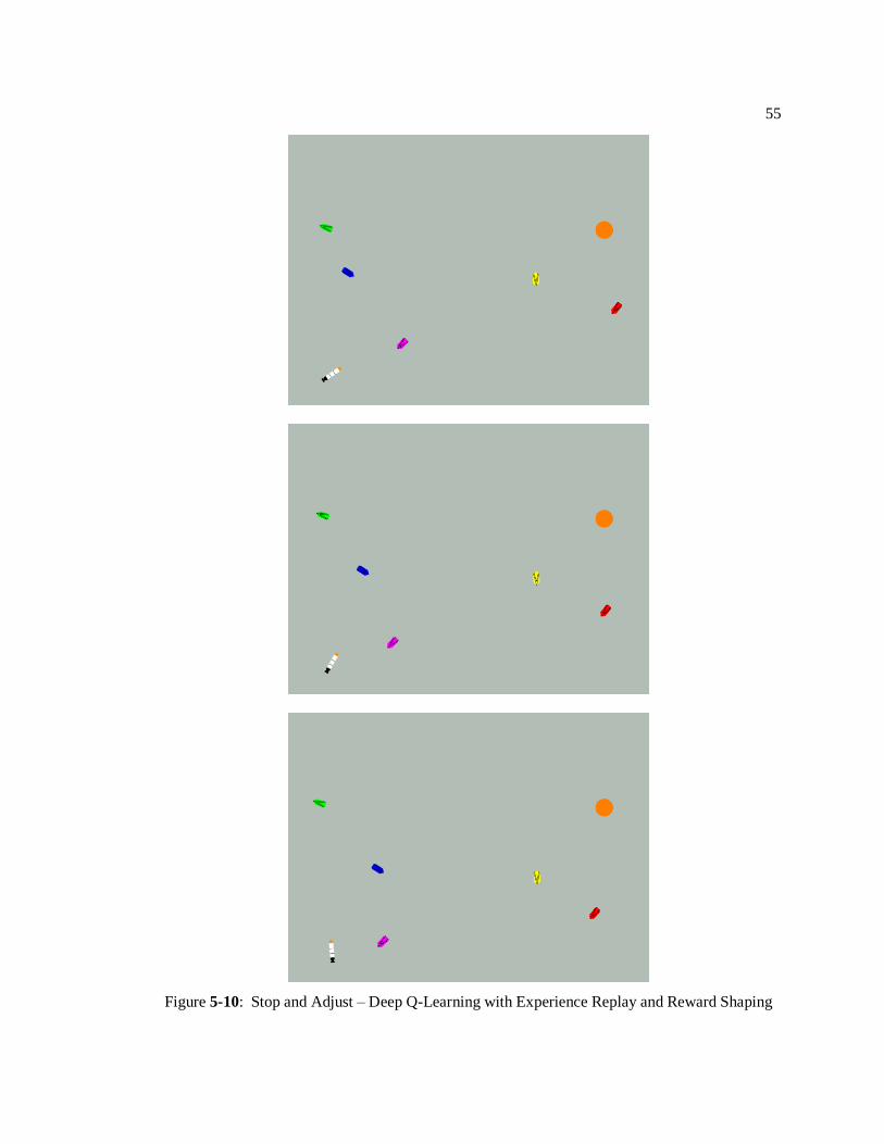
55

Figure 5-10: Stop and Adjust – Deep Q-Learning with Experience Replay and Reward Shaping

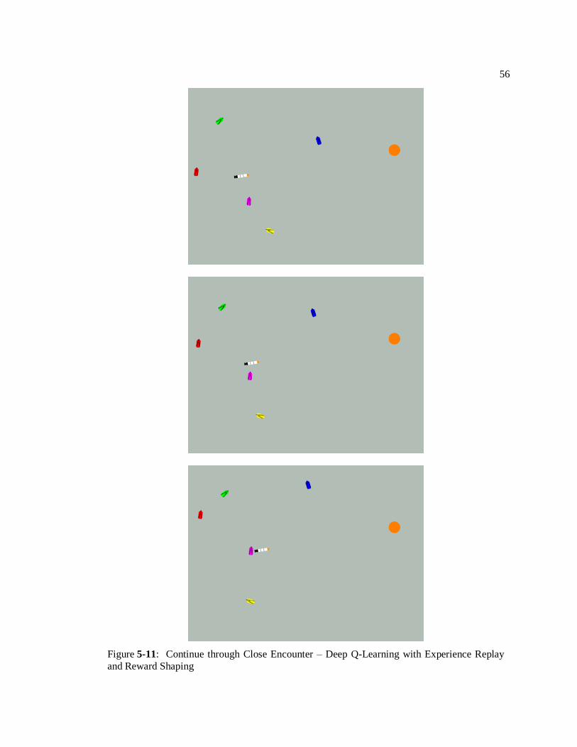
56

Figure 5-11: Continue through Close Encounter – Deep Q-Learning with Experience Replay

and Reward Shaping

57

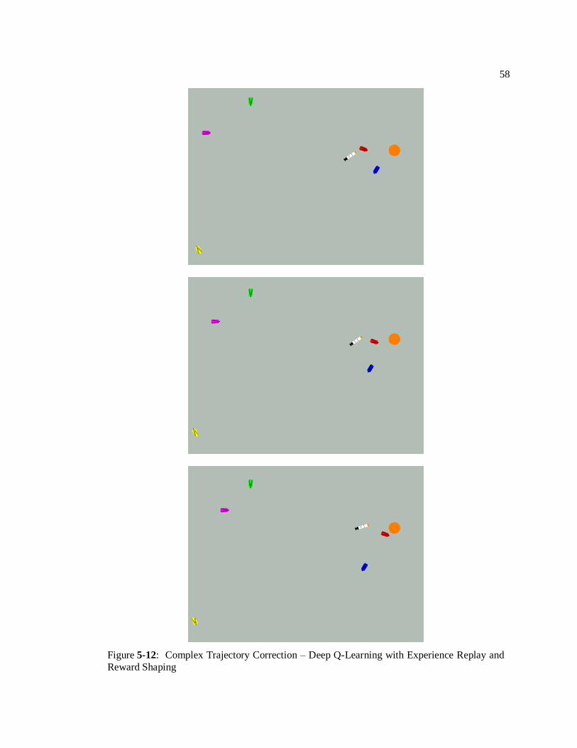
58

Figure 5-12: Complex Trajectory Correction – Deep Q-Learning with Experience Replay and

Reward Shaping

59

In Figure 5-10, shortly after beginning the episode, the UUV stops and rotates to

completely change its course. This behavior appears to occur when the UUV is trapped by two or

more (in this case, the blue and magenta) contacts in one of the corner regions of the

environment.

In Figure 5-11, it appears that the agent will again collide with the magenta contact.

However, the UUV appears to recognize that a collision will not occur and continues completely

linearly on its course. A collision did not occur.

In Figure 5-12, the UUV is close to the objective but is presented with potential collisions

with the blue and the red contacts. It performs a complex maneuver, dipping south and back

north to sequentially avoid both contacts and arrive successfully at the objective.

60

Catastrophic Forgetting from Extreme Shaping and Small Memory

The following example represents a failed training attempt of the Deep Q-Learning

network using both experience replay and reward shaping. In this scenario, the experience replay

buffer was limited to only 100,000 transitions. Additionally, the reward shaping schedule was

much more aggressive, attempting to anneal the collision penalty to -10,000 as shown in Table 5-

2.

This aggressive annealing, combined with a small replay buffer, caused the network to

diverge and forget its learned behavior. When the penalty for collision approached about -1,500,

the agent began to forget its ability to reach the objective. This is depicted in Figure 5-13.

Table 5-2: Reward Shaping Schedule – Catastrophic Forgetting

Episode Range Penalty for Detection

0 to 149,000 -100.0

150,000 to 799,999 -100.0 to -10,000.0 (linear decay)

800,000 to 1,000,000 -10,000.0

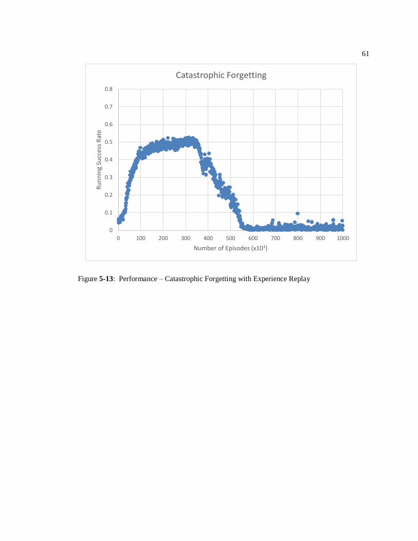
61

Figure 5-13: Performance – Catastrophic Forgetting with Experience Replay

0

0.1

0.2

0.3

0.4

0.5

0.6

0.7

0.8

0 100 200 300 400 500 600 700 800 900 1000

Ru

nn

ing

Succ

ess

Rat

e


Catastrophic Forgetting

62

Chapter 6

Discussion

Three variants of Deep Q-Learning were implemented in Chapter 5 and evaluated for the

problem of UUV navigation and contact avoidance.

The first implementation was that of traditional Q-Learning, while utilizing a neural

network as a function approximator for the action-value function. This implementation was

shown to suffer significantly from the phenomenon of catastrophic forgetting. Although a high

success rate was achieved during the training process, before the completion of training, the

unstable network diverged, inducing the agent to forget its ability to navigate properly, ending the

training sequence with poor performance. An early-stopping feature may have been able to

recover the performant network by rolling back the network to a state where high performance

was being achieved, before divergence. However, it may have been the case that the network

converged to a brittle, unstable local minimum that may not have generalized well at test time.

The second implementation augmented the first by adding experience replay memory.

This experience replay memory saves transitions experience by the agent to a large buffer. It

samples from this buffer in batches for training in an attempt to break the correlations between

successive transitions and in an attempt to train using past experiences to reinforce previous

behavior. The addition of a large buffer experience replay module enabled the Deep Q-Learning

algorithm to converge, without forgetting, for this task. The trained agent exhibited promising

behaviors indicating its ability to both navigate to the objective and avoid contacts. Both long-

approach and short-approach maneuvers were observed which enabled the agent to correct its

course, avoiding detection by the contacts.

63

Finally, the third implementation augmented the experience replay agent by shaping the

penalty for detection over time. After initial training, the penalty for detection was slowly

annealed, inducing the agent to value successful anti-detection measures more heavily. This

caused a small overall decrease in the performance metric for successfully reaching the objective

location. However, more advanced contact avoidance techniques were observed. For example,

the ability to stop and change course, the ability to continue linearly when a close encounter

would be out of the detection range, and the ability to perform advance trajectory corrections

when multiple contacts are approaching were observed. In addition to the successful training of

the reward shaping experience replay algorithm, when the detection penalty was annealed

significantly low, it was observed that this again causes the q-network to diverge.

Overall, these trials provide support for the use of reinforcement learning techniques in

the domain of maritime navigation and contact avoidance, even when lacking useful sensor data.

These algorithms were able to overcome the uncertainty presented by the environment and both

successfully navigate to the objective location while simultaneously avoiding detection by

moving contacts.

Possible Future Work

Use of Expanded Information

This thesis explored the extent to which autonomous navigation and contact avoidance is

possible given extremely limited access to sensor information. The results achieved used no

notion of absolute positioning, but rather only relative bearing information and speed

measurements. One potential extension of this work is to examine what to what extent learning is

possible in a richer environment. The UUV could be modelled with sensors enabling it to

64

accurately compute both the bearing and absolute distance to the contacts. Then, similar

procedures could be run to investigate this new array of information.

Evaluation of Additional Algorithms

The task of nautical navigation presents a very challenging and unique application of

reinforcement learning. Future work might extend the evaluation of RL algorithms beyond Q-

learning and Deep Q-learning to investigate other state of the art methods such as proximal policy

optimization (PPO) or an ensemble of task-oriented networks.

Proximal Policy Optimization

Proximal Policy Evaluation (PPO) is an algorithm developed by Schulman, et. al. at

OpenAI [31]. This algorithm is a policy gradient method which alternates between sampling data

from the environment and optimizing an objective function with stochastic gradient ascent. PPO

has been shown to be effective on many traditional reinforcement learning benchmarks and may

be appropriate for this task as well.

Ensemble of Networks

Another approach warranting examination is the use of an ensemble of Deep Q-Learning

networks. For example, a network could be separately trained for UUV navigation and another

separately trained for contact avoidance. An ensemble of these two networks may be better than

a single network jointly optimized for both tasks.

65

Additionally, ensembles of finer granularity could also be explored. For example, a

network for contact detection, a network for contact distance estimation, a network for proximity

detection, and a network for action proposition could all be combined to form a singular

algorithm for contact avoidance.

Application to 3D Simulation

Additional future work might involve re-training in a three-dimensional environment

which better models the real-world mechanics of navigation. Such a simulation might be built in

Unity or Unreal and used as both a front-end interface and as an environment from which to

sample data to emulate the state of the UUV.

Transfer Learning to Real-World Agent

Finally, an ambitious goal might be to develop a method to transfer the policies learned in

simulation to the decision making of a real-world vehicle. The problem at hand would involve

demonstrating that the trial and error processes and information learned therein in simulation

might aid a real vehicle in navigation. Can the negative feedback of learning be experienced in

simulation before applied in practicality? Direct transfer of simulated results to real-world

navigation would open up a whole new field of possibilities for transfer learning.

66

Chapter 7

Conclusion

This thesis explored, in simulation, the application of reinforcement learning to the

unique problem of maritime navigation and contact avoidance. This thesis built upon previous

work in the field through the introduction of dynamic, moving contacts, and the reduction of

information available for decision making. Operating under conditions with very limited sensory

input data, an unmanned underwater vehicle was induced to navigate to an objective in a

randomly generated environment while avoiding detection by moving contacts with high success

rate. The inherently sequential task of navigation and contact avoidance was not exempt from

catastrophic forgetting of the neural network function approximator. Measures to combat this

forgetting, including experience replay memory and reward shaping, were successful for this

problem. Overall, the simulated reinforcement learning agent demonstrated the ability to

navigate successfully to its objective while performing advanced contact avoidance maneuvers.

This thesis opens up the problem of UUV navigation and contact avoidance for further

examination under different constraints, powered by different algorithms, and in more advanced

simulations or wet settings.

67

Bibliography

[1] A. Krizhevsky and G. E. Hinton, “ImageNet Classification with Deep Convolutional

Neural Networks,” pp. 1–9.

[2] Y. Lecun, Y. Bengio, and G. Hinton, “Deep learning,” Nature, vol. 521, no. 7553. pp.

436–444, 2015.

[3] V. Mnih and D. Silver, “Playing Atari with Deep Reinforcement Learning,” pp. 1–9.

[4] D. Silver, A. Huang, C. J. Maddison, A. Guez, L. Sifre, G. Van Den Driessche, J.

Schrittwieser, I. Antonoglou, V. Panneershelvam, M. Lanctot, S. Dieleman, D. Grewe, J.

Nham, N. Kalchbrenner, I. Sutskever, T. Lillicrap, M. Leach, and K. Kavukcuoglu,

“Mastering the game of Go with deep neural networks and tree search,” Nature, vol. 529,

no. 7585, pp. 484–489, 2016.

[5] D. Silver, J. Schrittwieser, K. Simonyan, I. Antonoglou, A. Huang, A. Guez, T. Hubert, L.

Baker, M. Lai, A. Bolton, Y. Chen, T. Lillicrap, F. Hui, L. Sifre, G. Van Den Driessche,

T. Graepel, and D. Hassabis, “Mastering the game of Go without human knowledge,”

Nature, vol. 550, no. 7676, pp. 354–359, 2017.

[6] R. Yu, Z. Shi, C. Huang, T. Li, and Q. Ma, “Deep Reinforcement Learning Based Optimal

Trajectory Tracking Control of Autonomous Underwater Vehicle,” Chineese Control

Conf., pp. 4958–4965, 2017.

[7] I. Carlucho, M. De Paula, S. Wang, Y. Petillot, and G. G. Acosta, “Adaptive low-level

control of autonomous underwater vehicles using deep reinforcement learning,” Rob.

Auton. Syst., vol. 107, pp. 71–86, 2018.

[8] H. Wu, S. Song, S. Member, K. You, S. Member, and C. Wu, “Depth Control of Model-

Free AUVs via Reinforcement Learning,” pp. 1–12, 2018.

68

[9] C. Gaskett, D. Wettergreen, and A. Zelinsky, “Reinforcement Learning applied to the

control of an Autonomous Underwater Vehicle.”

[10] P. Ed-Fakdi, A., Carreras, M., Palomeras, N., Ridao, “Autonomous Underwater Vehicle

Control using Reinforcement Learning Policy Search Methods,” Ocean. - Eur., pp. 793–

798, 2005.

[11] C. Wang, L. Wei, Z. Wang, and M. Song, “Reinforcement Learning-Based Multi-AUV

Adaptive Trajectory Planning for Under-Ice Field Estimation,” Sensors, pp. 1–19, 2018.

[12] Y. Sun, J. Cheng, G. Zhang, and H. Xu, “Mapless Motion Planning System for an

Autonomous Underwater Vehicle Using Policy Gradient-based Deep Reinforcement

Learning,” J. Intellegent Robot. Syst., 2019.

[13] R. Glatt, A. Helena, and R. Costa, “Improving Deep Reinforcement Learning with

Knowledge Transfer ∗,” pp. 5036–5037.

[14] D. L. Moreno, C. V Regueiro, and R. Iglesias, “Using Prior Knowledge to Improve

Reinforcement Learning in Mobile Robotics,” 1996.

[15] K. R. Dixon, R. J. Malak, and P. K. Khosla, “Incorporating Prior Knowledge and

Previously Learned Information into Reinforcement Learning Agents,” 2000.

[16] R. Sutton and A. Barto, Reinforcement Learning, An Introduction. .

[17] P.-R. T. Guo, X. P., hernandez-Lerma, O., “A Survey of Recent Results on Coninuous-

Time Markov Decision Processes,” vol. 14, no. 2, pp. 177–257, 2006.

[18] X. Guo, “Continuous-Time Markov Decision Processes with Discounted Rewards : The

Case of Polish Spaces,” vol. 32, no. 1, pp. 73–87, 2019.

[19] F. E. T. Al, Z. Feng, R. Dearden, N. Meuleau, and R. Washington, “Dynamic

Programming for Structured Continuous Markov Decision Problems,” pp. 154–161, 2004.

[20] G. Tesauro, “Temporal Difference Learning and TD-Gammon.”

[21] D. Silver, T. Hubert, J. Schrittwieser, I. Antonoglou, M. Lai, A. Guez, M. Lanctot, L.

69

Sifre, D. Kumaran, T. Graepel, T. Lillicrap, K. Simonyan, and D. Hassabis, “Mastering

Chess and Shogi by Self-Play with a General Reinforcement Learning Algorithm arXiv :

1712 . 01815v1 [ cs . AI ] 5 Dec 2017,” pp. 1–19.

[22] G. A. I. Princeton, “Provably Efficient Maximum Entropy Exploration,” pp. 1–13.

[23] P. Auer, “Using Confidence Bounds for Exploitation-Exploration Trade-offs,” vol. 3, pp.

397–422, 2002.

[24] D. J. Russo, B. Van Roy, and A. Kazerouni, “A Tutorial on Thompson Sampling,” pp. 1–

96.

[25] C. J. C. H. Watkins, “Learning from Delayed Rewards.” 1989.

[26] C. J. C. H. Watkins, “Q-Learning A Technical Note,” vol. 292, pp. 279–292, 1992.

[27] F. S. Melo, “Convergence of Q-learning: A simple proof,” Inst. Syst. Robot. Tech. Rep,

pp. 1–4, 2007.

[28] J. Kirkpatrick, R. Pascanu, N. Rabinowitz, J. Veness, and G. Desjardins, “Overcoming

catastrophic forgetting in neural networks,” 2015.

[29] J. Keller, “Navy undersea warfare experts ask OceanServer to refurbish Iver2 research

UUV,” Military and Aerospace Electronics, 2014. .

[30] “Sonar,” University of Rhode Island and Inner Space Center, 2017. .

[31] J. Schulman, F. Wolski, P. Dhariwal, A. Radford, and O. Klimov, “Proximal Policy

Optimization Algorithms,” pp. 1–12.

70

Appendix A

Summary of Notation and Acronyms

Table A-1: Summary of Notation

𝛼 learning rate

𝒜 set of all possible actions

𝑎, 𝐴, 𝑎𝑡 , 𝐴𝑡 current action

𝒟 experience replay memory

𝜖 rate of exploration

𝛾 discount factor

𝐺, 𝐺𝑡 , 𝐺𝑇 cumulative future reward

𝑀 size of experience replay memory

𝑁 number of training episodes

𝜋 policy

𝜋∗ optimal policy

𝜋(𝑎|𝑠) policy function

𝜋∗(𝑎|𝑠) optimal policy function

𝑞, 𝑄, 𝑞(𝑠, 𝑎) action-value function

𝑞𝜋 , 𝑄𝜋 , 𝑞𝜋(𝑠, 𝑎) action-value function, following policy 𝜋

𝑞∗, 𝑄∗, 𝑞∗(𝑠, 𝑎) optimal action-value function

ℝ set of all real, scalar numbers

𝑟, 𝑅, 𝑟𝑡 , 𝑅𝑡 current reward

𝒮 set of all possible states

𝑠, 𝑆, 𝑠𝑡 , 𝑆𝑡 current state

𝑠′, 𝑆′ next state

𝑇 number of timesteps/transitions

𝑣, 𝑣(𝑠) state-value function

𝑣𝜋 , 𝑣𝜋(𝑠) state-value function, following policy 𝜋

𝑣∗, 𝑣∗(𝑠) optimal state-value function

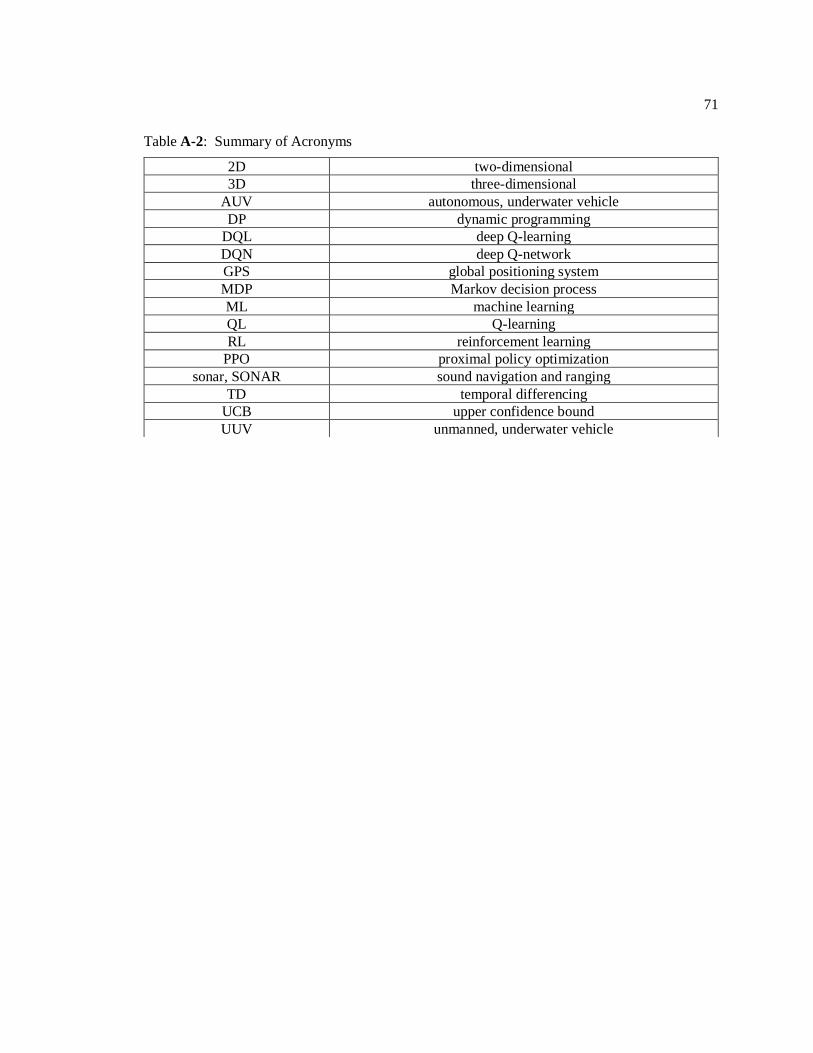
71

Table A-2: Summary of Acronyms

2D two-dimensional

3D three-dimensional

AUV autonomous, underwater vehicle

DP dynamic programming

DQL deep Q-learning

DQN deep Q-network

GPS global positioning system

MDP Markov decision process

ML machine learning

QL Q-learning

RL reinforcement learning

PPO proximal policy optimization

sonar, SONAR sound navigation and ranging

TD temporal differencing

UCB upper confidence bound

UUV unmanned, underwater vehicle

72

Appendix B

Code

Complete source code will not be released. Below are files documenting the primary

reinforcement learning modules.

ReinforcementLearningModule.py

import random

import time

from abc import ABC, abstractmethod

class ReinforcementLearningModule(ABC):

def __init__(self, num_episodes, train, discount_factor=0.9, learning_rate=0.1):

self.discount_factor = discount_factor

self.learning_rate = learning_rate

self.num_episodes = num_episodes

self.episode_number = 0

self.will_train = train

self.model = self.load_model()

self.start_time = time.time()

self.success_history = []

random.seed()

self.run_id = ''.join(random.sample('ABCDEFGHIJKLMNOPQRSTUVWXYZ', 5))

@abstractmethod

def load_model(self):

pass

@abstractmethod

def save_model(self):

pass

@staticmethod

@abstractmethod

def generate_new_model():

pass

@abstractmethod

def get_optimal_action_for_state(self, state_list, action_options):

"""

Returns the optimal action.

"""

pass

@abstractmethod

def get_maximum_q_for_state(self, state_list):

"""

Returns the maximum Q value associated with this state.

"""

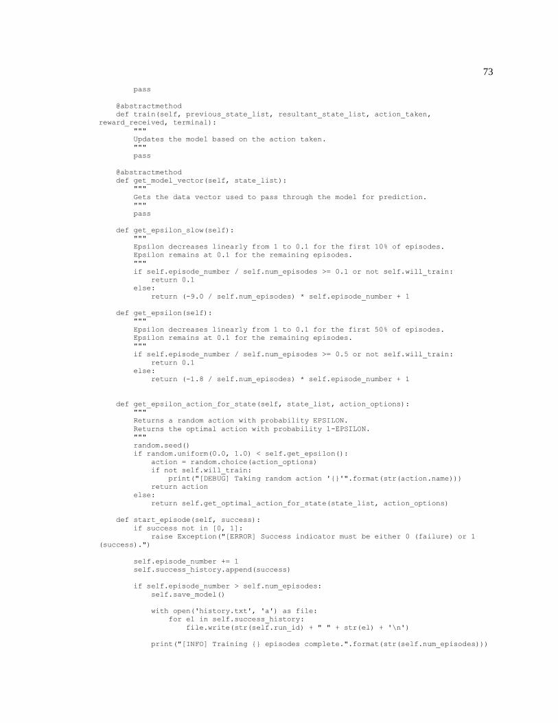
73

pass

@abstractmethod

def train(self, previous_state_list, resultant_state_list, action_taken,

reward_received, terminal):

"""

Updates the model based on the action taken.

"""

pass

@abstractmethod

def get_model_vector(self, state_list):

"""

Gets the data vector used to pass through the model for prediction.

"""

pass

def get_epsilon_slow(self):

"""

Epsilon decreases linearly from 1 to 0.1 for the first 10% of episodes.

Epsilon remains at 0.1 for the remaining episodes.

"""

if self.episode_number / self.num_episodes >= 0.1 or not self.will_train:

return 0.1

else:

return (-9.0 / self.num_episodes) * self.episode_number + 1

def get_epsilon(self):

"""

Epsilon decreases linearly from 1 to 0.1 for the first 50% of episodes.

Epsilon remains at 0.1 for the remaining episodes.

"""

if self.episode_number / self.num_episodes >= 0.5 or not self.will_train:

return 0.1

else:

return (-1.8 / self.num_episodes) * self.episode_number + 1

def get_epsilon_action_for_state(self, state_list, action_options):

"""

Returns a random action with probability EPSILON.

Returns the optimal action with probability 1-EPSILON.

"""

random.seed()

if random.uniform(0.0, 1.0) < self.get_epsilon():

action = random.choice(action_options)

if not self.will_train:

print("[DEBUG] Taking random action '{}'".format(str(action.name)))

return action

else:

return self.get_optimal_action_for_state(state_list, action_options)

def start_episode(self, success):

if success not in [0, 1]:

raise Exception("[ERROR] Success indicator must be either 0 (failure) or 1

(success).")

self.episode_number += 1

self.success_history.append(success)

if self.episode_number > self.num_episodes:

self.save_model()

with open('history.txt', 'a') as file:

for el in self.success_history:

file.write(str(self.run_id) + " " + str(el) + '\n')

print("[INFO] Training {} episodes complete.".format(str(self.num_episodes)))

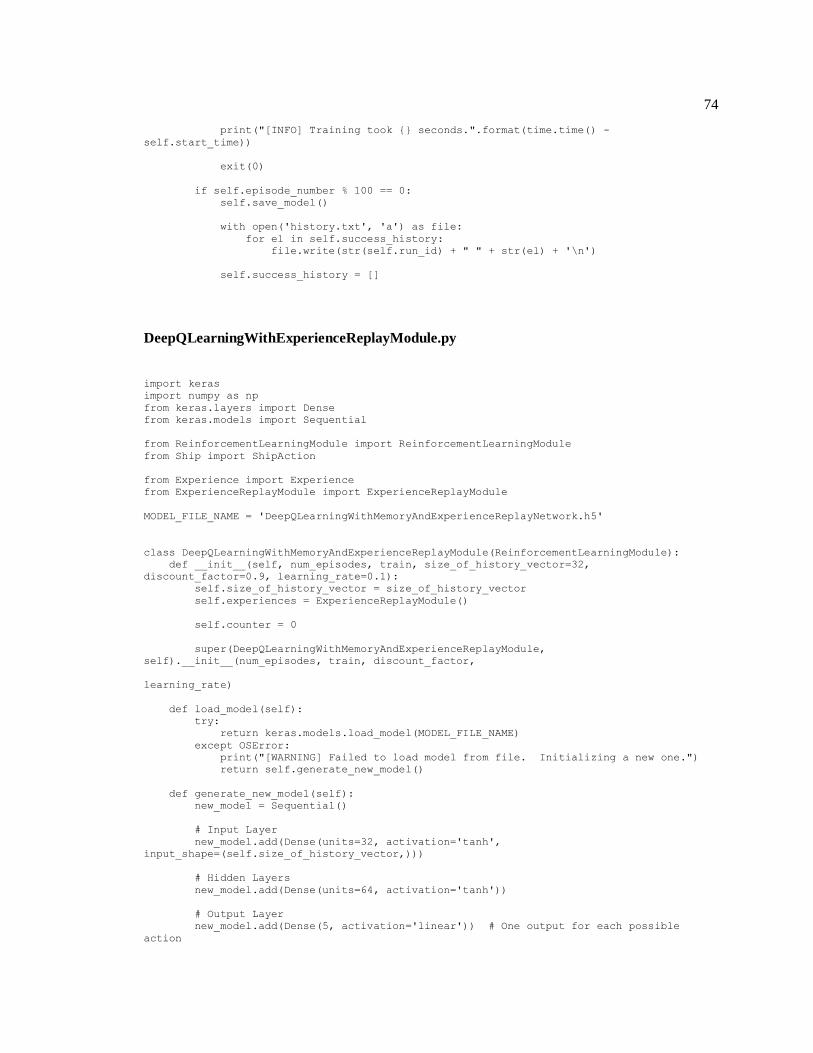
74

print("[INFO] Training took {} seconds.".format(time.time() -

self.start_time))

exit(0)

if self.episode_number % 100 == 0:

self.save_model()

with open('history.txt', 'a') as file:

for el in self.success_history:

file.write(str(self.run_id) + " " + str(el) + '\n')

self.success_history = []

DeepQLearningWithExperienceReplayModule.py

import keras

import numpy as np

from keras.layers import Dense

from keras.models import Sequential

from ReinforcementLearningModule import ReinforcementLearningModule

from Ship import ShipAction

from Experience import Experience

from ExperienceReplayModule import ExperienceReplayModule

MODEL_FILE_NAME = 'DeepQLearningWithMemoryAndExperienceReplayNetwork.h5'

class DeepQLearningWithMemoryAndExperienceReplayModule(ReinforcementLearningModule):

def __init__(self, num_episodes, train, size_of_history_vector=32,

discount_factor=0.9, learning_rate=0.1):

self.size_of_history_vector = size_of_history_vector

self.experiences = ExperienceReplayModule()

self.counter = 0

super(DeepQLearningWithMemoryAndExperienceReplayModule,

self).__init__(num_episodes, train, discount_factor,

learning_rate)

def load_model(self):

try:

return keras.models.load_model(MODEL_FILE_NAME)

except OSError:

print("[WARNING] Failed to load model from file. Initializing a new one.")

return self.generate_new_model()

def generate_new_model(self):

new_model = Sequential()

# Input Layer

new_model.add(Dense(units=32, activation='tanh',

input_shape=(self.size_of_history_vector,)))

# Hidden Layers

new_model.add(Dense(units=64, activation='tanh'))

# Output Layer

new_model.add(Dense(5, activation='linear')) # One output for each possible

action

75

# Compile Model

new_model.compile(loss='mse', optimizer='adam', metrics=['mae'])

return new_model

def save_model(self):

self.model.save(MODEL_FILE_NAME)

def get_optimal_action_for_state(self, state_list, action_options):

optimal_action = None

optimal_value = None

state_array = self.get_model_vector(state_list)

q_values = self.model.predict(state_array).tolist()[0]

for index in range(len(q_values)):

value = q_values[index]

if optimal_value is None or optimal_value < value:

if ShipAction(index) in action_options:

optimal_value = value

optimal_action = ShipAction(index)

if not self.will_train:

print("[DEBUG] Operating on state array: {}".format(state_array.tolist()[0]))

print("[DEBUG] Taking action '{}' from Q Values:

{}".format(str(optimal_action.name), str(q_values)))

if optimal_action is None:

raise Exception("No action decision.")

else:

return optimal_action

def get_maximum_q_for_state(self, state_list):

state_array = self.get_model_vector(state_list)

q_values = self.model.predict(state_array)

return np.max(q_values)

def train(self, previous_state_list, resultant_state_list, action_taken,

reward_received, terminal):

new_experience = Experience(previous_state_list, action_taken, reward_received,

resultant_state_list, terminal)

self.experiences.add_experience(new_experience)

self.counter += 1

if self.counter % 1000 == 0:

batch_size = 2000

batch_experiences =

self.experiences.sample_experiences(number_sampled=batch_size)

forward = []

back = []

for experience in batch_experiences:

previous_array = self.get_model_vector(experience.initial_state)

max_q = self.get_maximum_q_for_state(experience.resultant_state)

target_vector = self.model.predict(previous_array)[0]

if experience.terminal:

target = experience.reward

else:

target = experience.reward + self.discount_factor * max_q

target_vector[experience.action.value] = target

target_vector = target_vector.reshape((1, 5))

forward.append(previous_array)

back.append(target_vector)

forward_array = np.concatenate(forward)

76

back_array = np.concatenate(back)

self.model.fit(forward_array, back_array, epochs=10, batch_size=128,

verbose=0)

def get_model_vector(self, state_list):

return np.array(state_list).reshape((1, self.size_of_history_vector)

Steven Davis [email protected] | (412) 398-8883

Permanent Address

905 Monastery View Bethel Park, PA 15102

Education The Pennsylvania State University

Schreyer Honors College Dual Bachelor of Science and Master of Science in Computer Engineering

May 2019

Bethel Park Senior High School Valedictorian and National Honor Society President

May 2015

Experience Capital One – Software Engineering Intern June 2018 – August 2018

• Rearchitected, refactored, and unit tested significant portions of the CreditWise iOS application

• Utilized MVVM architecture and reactive programming paradigms to modernize the application and increase testability

• Catered to the diverse needs of a 26+ million user customer base

Penn State Dance Marathon – Technology Director April 2017 – April 2018

• Oversaw 3 teams of 5-7 software developers, utilizing and instilling agile/scrum development principles for continuous delivery systems

• Contributed to the development of enterprise-scale management tools

• Architected new software that reduced spectator wait time from 10.0 to 1.5 hours

• Served on the executive committee and collaborated with other student leaders to ensure the success and sustainability of our multimillion-dollar, 16,500-student-strong philanthropy

J.P. Morgan Chase & Co. – Software Development Intern / Technology Analyst June 2017 – August 2017

• Leveraged Java, SQL, Bash scripting, the Spring Boot Framework, and other technologies to contribute to a web application for meta-data registration and data ingestion into an enterprise-scale data warehouse

• Experienced full-stack enterprise software engineering including database architecture, database access, REST API creation, backend development, and front-end development

• Developed as a member of a scrum team of interns and full-time employees

Applied Research Laboratory – Graduate Assistant August 2017 – present

• Benchmarked and investigated the Elastic stack (Logstash, Elasticsearch, Kibana)

• Evaluated reinforcement learning algorithms for autonomous underwater vehicle navigation

Penn State Dance Marathon Technology Committee – Pass System Developer Aug. 2016 – April 2017

• Used Python on top of Django in a Unix development environment to program building management and floor access software for a building that seats over 15,000 people

• Operated as a part of a team in three-week agile software development sprints

Leadership and Service

Leadership JumpStart – Teaching Assistant March 2017 – present Boy Scouts of America – Eagle Scout May 2010 – Aug. 2015

• Designed, organized and led the construction of a pavilion at a local elementary school

• Recorded all financial transactions for over 150 members; accounted for over $400,000 during term

Skills Languages: Python, Java, Swift, C, SQL, Bash, MATLAB, HTML5 Technologies: Git, Django Web Framework, sci-kit learn, Reactive(Swift), Spring and Spring Boot

Frameworks, Bootstrap, REST, Unix Environments Honors and Awards

Lockheed Martin Scholar, September 2017 BP Scholar, August 2016 4th Place CODE PSU Competition: Intermediate Tier, March 2016 President’s Freshman Award, Spring 2016 Dean’s List, Fall 2015, Spring 2016, Fall 2016, Spring 2017, Fall 2017, Spring 2018, Fall 2018

Documents

MARITIME NAVIGATION AND CONTACT AVOIDANCE THROUGH