MARITAL HISTORIES, GENDER, AND FINANCIAL SECURITY

IN LATE MID-LIFE: EVIDENCE FROM FOUR COHORTS IN THE HEALTH AND RETIREMENT STUDY

Amelia Karraker and Cassandra Dorius

CRR WP 2016-4

July 2016

Center for Retirement Research at Boston College Hovey House

140 Commonwealth Ave Chestnut Hill, MA 02467

Tel: 617-552-1762 Fax: 617-552-0191 http://crr.bc.edu

Amelia Karraker and Cassandra Dorius are assistant professors at Iowa State University. The research reported herein was performed pursuant to a grant from the U.S. Social Security Administration (SSA) funded as part of the Retirement Research Consortium. The opinions and conclusions expressed are solely those of the authors and do not represent the opinions or policy of SSA, any agency of the federal government, Iowa State University, or Boston College. Neither the United States Government nor any agency thereof, nor any of their employees, makes any warranty, express or implied, or assumes any legal liability or responsibility for the accuracy, completeness, or usefulness of the contents of this report. Reference herein to any specific commercial product, process or service by trade name, trademark, manufacturer, or otherwise does not necessarily constitute or imply endorsement, recommendation or favoring by the United States Government or any agency thereof. © 2016, Amelia Karraker and Cassandra Dorius. All rights reserved. Short sections of text, not to exceed two paragraphs, may be quoted without explicit permission provided that full credit, including © notice, is given to the source.

About the Steven H. Sandell Grant Program

This paper received funding from the Steven H. Sandell Grant Program for Junior Scholars in Retirement Research. Established in 1999, the Sandell program’s purpose is to promote research on retirement issues by scholars in a wide variety of disciplines, including actuarial science, demography, economics, finance, gerontology, political science, psychology, public administration, public policy, sociology, social work, and statistics. The program is funded through a grant from the Social Security Administration (SSA). For more information on the Sandell program, please visit our website at: http://crr.bc.edu/?p=9570, send e-mail to crr@bc.edu, or call (617) 552-1762.

About the Center for Retirement Research

The Center for Retirement Research at Boston College, part of a consortium that includes parallel centers at the University of Michigan and the National Bureau of Economic Research, was established in 1998 through a grant from the Social Security Administration. The Center’s mission is to produce first-class research and forge a strong link between the academic community and decision-makers in the public and private sectors around an issue of critical importance to the nation’s future. To achieve this mission, the Center sponsors a wide variety of research projects, transmits new findings to a broad audience, trains new scholars, and broadens access to valuable data sources.

Center for Retirement Research at Boston College

Hovey House 140 Commonwealth Ave Chestnut Hill, MA 02467

Tel: 617-552-1762 Fax: 617-552-0191 http://crr.bc.edu

Affiliated Institutions: The Brookings Institution

Massachusetts Institute of Technology Syracuse University

Urban Institute

Abstract

Marital status is an established predictor of financial well-being in later life, with

continuously married people enjoying considerable economic benefits that accumulate over the

life course, contrasting sharply with the economic vulnerabilities faced by divorced, widowed, or

never-married individuals. Although prior work suggests that marital histories—including the

number and sequencing of past and present unions and dissolutions—have become more

complex for more recent cohorts, the economic ramifications of this demographic shift are

unclear. Further, how shifts away from continuous marriage will impact women’s financial

security in later life is unknown. Using data from the Health and Retirement Study, we examine

cohort and gender variation in the relationship between elaborated marital history measures and

financial security at ages 51-56, when wealth and earnings are at or near lifetime peaks. We

examine three financial measures (negative, zero, and positive wealth; positive wealth levels;

earnings) that capture distinct components of financial security as individuals approach

retirement.

The paper found that:

• Middle Baby Boomers born in the mid- to late-1950s differ from older cohorts born in

the mid- to late-1930s by both marital history and financial security measures.

• Middle Baby Boomers are more likely to have negative wealth (i.e. debt) or zero wealth,

and those who have positive wealth have lower levels of wealth. On the other hand,

Middle Baby Boomers working full-time have higher earnings than earlier cohorts,

especially women.

• More recent cohorts are less likely to be continuously married than previous cohorts.

• The relationship between marital history and financial security depends on whether

wealth or earnings is examined. Specifically, the economic benefits of continuous

marriage are more pronounced for wealth than earnings.

The policy implications of the findings are:

• Social Security policy changes might consider the increasing complexity in marital

histories of more recent cohorts.

• Greater attention can be paid to two growing segments of adults in late mid-life: those

with zero wealth and those in debt, who are approaching retirement in a particularly

precarious position. They are more likely to rely on Social Security and may be

particularly adversely affected if proposed benefit cuts were enacted.

Introduction

Marriage and financial resources are intertwined throughout life, with continuously

married people reporting higher net wealth, assets, and incomes and larger pensions and fewer

draws on Supplemental Security Income or welfare (e.g., Holden and Smock 1991, Johnson and

Favreault 2004). Beyond a single point in time, the marital wealth advantage is hypothesized to

accumulate so that married couples accrue increasingly large economic returns from their union

as the years pass, while unmarried people see less significant gains, leading to ever-growing

disparities between families (Hirschl, Altobelli, and Rank 2003). Individuals’ marital histories—

which we define as the sequencing of marital status and the duration of current and past

relationships—have also become less stable and more complex over the second half of the

twentieth century. Individuals in later-born birth cohorts are more likely to experience divorce

and cohabitation and are less likely to ever marry compared to their earlier-born counterparts

(Cherli, 2010). While there is evidence to suggest that financial security in later life varies by

cohort, with more-recent cohorts having more total wealth (Addo and Lichter 2013), it is not

known what potentially changing role marital history plays in inter-cohort differences in

financial security. Furthermore, given women’s increasing economic parity with men over time,

it is unclear how the relationship between marital history and financial security will vary by

gender within and between cohorts. We use the Health and Retirement Study (HRS) to examine

inter-cohort and gender variation in the relationship between marital history and financial

security in late mid-life (ages 51-56), a forerunner of economic security in retirement (Collins,

Scholz, and Seshadri 2013).

Background

There are many reasons why marriage and financial security are positively associated

with one another. In particular, resource pooling may lead to greater financial security among

married couples because marital homes have more potential workers to generate shared incomes,

a greater ability to divide labor in ways that maximize family income, and they enjoy the benefits

from economies of scale associated with additional family members (Hirschl et al. 2003).

Likewise, married people may reinforce positive shared financial goals with their spouses, such

as saving for retirement or maintaining steady employment, which are tied to greater financial

assets and earnings in later life. Further, the financial benefits of continuous marriage—relative

2

to other marital histories—tend to be larger later in life as individuals have more opportunities to

accrue advantages through marriages of longer duration (Addo and Lichter 2013). Depending on

an individual’s complete marital history, he or she may be more or less financially secure

heading into retirement (Holden and Smock 1991).

Despite the importance of marital history for financial security in later life, prior work

has been limited by a reliance on basic measures of marital status, financial security, or both.

Basic measures of marital status (i.e., current marital status or continuously married versus all

else) used in some previous studies cannot distinguish between important sequences and

durations of events. This approach is problematic because the mechanisms that link marriage

and financial security may be contingent on detailed marital histories. For example, prior

research by Wilmoth and Koso (2002) found that the relationship between total wealth and

marital dissolution depends on whether it is the first or second marriage being dissolved, with

larger total wealth reductions for second marriages. Although important insights have been

gleaned using elaborated marital histories in some prior research (e.g., Addo and Lichter 2013,

Wilmoth and Koso 2002), this work has generally been limited to an assessment of total wealth,

which captures only one facet of the many ways in which marriage may influence financial

security in later life.

Beyond the importance of assessing elaborated marital histories and multidimensional

measures of financial security, it also is important to consider the population being looked at and

how demographic characteristics might affect the basic relationship between marriage and

economic wellbeing. Due to data limitations, prior scholarship has been unable to examine the

most recent cohorts of adults approaching retirement—Middle Baby Boomers. Information on

the determinants of financial security among this cohort is needed for at least two reasons. First,

more recently born cohorts differ from earlier-born cohorts along financial measures, such as

more limited access to defined-benefit plans (Harrington Meyer and Herd 2007), making an

understanding of individuals’ own financial resources more important than ever for retirement

income policy. Second, more recently born cohorts have experienced lower rates of continuous

marriage and higher rates of never marrying, which may leave later-born individuals financially

vulnerable because they have fewer spousal resources to draw from in older ages.

Although marriage is thought to benefit both partners, it influences men and women in

distinct ways, with women paying a higher economic price for divorce, separation, and

3

widowhood compared with men (Holden and Smock 1991). Moreover, women are less likely to

remarry following a divorce (Cherlin 2010), which may doubly disadvantage older wives relative

to their husbands because they not only pay a higher price for divorcing, they are less likely to

recoup their losses by remarrying. Furthermore, because men make more money than women

and are also more likely to have access to pensions, men are more likely to achieve financial

security and live above the poverty line in later life compared to women, regardless of marital

status (Harrington Meyer and Herd 2007). And though women routinely face wage penalties for

both marriage and motherhood that men do not experience (e.g., Holden and Smock 1991),

women may actually receive more long-term wealth benefits from marriage than men—largely

because women are less likely than men to achieve affluence without getting and staying married

(Hirschl et al. 2003)—though it is unknown how this may vary by cohort given women’s

increasingly complex marital histories on one hand, and growing economic parity with men on

the other.

To address these limitations, we use data from the HRS to examine the relationship

between detailed marital histories and three measures of financial wellbeing (negative, zero, and

positive wealth; positive wealth levels; and earnings levels) for men and women. We include

cohorts of older Americans who have experienced vastly different family forming behaviors: the

original HRS Cohort, War Babies, Early Baby Boomers, and Middle Baby Boomers. This

project presents a more complete picture of how family complexity influences financial security

in pre-retirement, as well as how financial security may be changing by gender and across

cohorts, information that is critically important to researchers and policymakers.

Data

We use data from the HRS to examine inter-cohort and gender variation in the

relationship between marital history and financial security in later life. The HRS is a nationally

representative, prospective panel study of Americans ages 50 and older. Our analysis is based on

the RAND HRS files (version O), a publicly available, cross-wave harmonized version of HRS,

which facilitates direct comparison of different waves of the data and includes current and

retrospective marital histories. Our analysis includes four cohorts of HRS respondents,

4

comprised of: members of the original HRS cohort1 (born 1936-1941, first collected 1992), the

War Babies (born 1942-1947, first collected 1998), the Early Baby Boomers (born 1948-1953,

first collected 2004), and the Middle Baby Boomers (born 1954-1959, first collected 2010). We

examine each cohort in the first wave that data was collected for a specific cohort, at ages 51 to

56, when income and assets are frequently at or near lifetime peaks (Lee, Lee, and Mason 2008).

This approach also enables us to consider the how differences in marital histories may have

unique financial benefits and consequences for various cohorts at the same stage of the life

course, allowing us to more clearly differentiate between age and cohort effects. We return to

the issue of period effects in our discussion of key findings.

Our three dependent variables capture distinctive facets of financial well-being that have

important but discrete implications for financial security as individuals’ transitions into

retirement ages. Our first measure is an indicator for whether a respondent’s household has

negative, zero, or positive total wealth. Wealth is a critical component of retirement savings

(Poterba 2014). Whether someone is in debt (i.e. negative wealth), has zero wealth, or some

level of positive wealth is indicative of basic financial security and those with zero and even

negative wealth are the most disadvantaged and arguably ill-prepared for retirement. Our second

measure is positive wealth, which reflects in part the adequacy of savings for retirement. Our

third measure is positive earned income, restricted to those working full-time (35+ hours per

week, 36+ weeks per year). We focus on earned income rather than income from other sources

(such as investments), because it more accurately reflects labor force attachment than other types

of income, helps determine Social Security payments, and provides more conceptual and

empirical clarity from wealth than other types of income (which may be derived from wealth in

the form of annuities, for example). We also briefly discuss variation in employment in the

Discussion section.

Our household wealth measure is based on the sum of the value of: primary residence;

secondary residence; other real estate; vehicles; businesses; IRA and Keogh accounts; stocks,

mutual funds, and investment trusts; checking, savings, and money market accounts; CDs,

government savings bonds, and T-bills; bonds and bond funds, and all other savings less the

1 The full original HRS cohort includes individuals born between 1931 and 1941. In order to make our original HRS sample comparable to other cohorts who are observed at ages 51-56, we restrict our HRS sample to those ages 51-56 at baseline (1992), and thus exclude HRS cohort members born 1931-1935 who were ages 57-61 at baseline.

5

value of: all mortgages and land contracts for primary residence; other home loans for primary

residence; all mortgages and land contracts for secondary residence; and other debts. Reports of

wealth fell along a continuum of negative to positive wealth. For the multinomial assessments of

wealth, negative wealth was coded as 1 for any person with a total household wealth below zero

(8 percent of the sample). Zero wealth was coded as 1 for any person whose total household

wealth equaled exactly zero (4 percent of the sample). Positive wealth was coded as 1 for any

person whose total household wealth exceeded zero (88 percent of the sample). For our linear

assessments of positive wealth, we included only those individuals who reported wealth of more

than 1 dollar.

Earned income reflects the reported income of the respondent from the following sources:

wages and salary; bonuses, overtime pay, commissions, and tips; second job or military reserve

income’ professional practice and trade income.

For both earnings and wealth, missing values are imputed by RAND using bracket

unfolding techniques and imputation algorithms (see Hurd, Meijer, Moldoff, and Rohwedder,

forthcoming). For positive wealth and earnings, we convert positive nominal earnings and

wealth for each year into 2016 dollars using Consumer Price Index multipliers provided by the

U.S. Bureau of Labor Statistics (2016). Given the skewness of both measures, we use a log

transformation of each. Finally, we top code the 99th percentile of both wealth and earnings to

reduce the effect of influential observations and leverage points, as suggested by Addo and

Lichter (2013).

Marital history measures are based on current and retrospective reports of relationship

status in each cohort’s respective baseline wave (when each cohort is between ages 51 and 56).

Prior research has found that detailed marital histories have statistical and substantive advantages

over basic marital histories for predicting wealth differentials at pre-retirement ages in the

original HRS cohort (Wilmoth and Koso 2002). Our measure of marital history is assessed with

17 elaborated marital history dummies of mutually-exclusive relationship sequences that capture

the full range of experiences across the four cohorts in our study. Thirteen of these sequences

were originally documented by Wilmoth and Koso (2002) and describe first the current status

and then the prior status, including: continuously married (reference); never married; cohabiting

never married; cohabiting, divorced or widowed once; cohabiting, divorced or widowed twice;

single, divorced once; single, widowed once; single, divorced twice; remarried, divorced once;

6

remarried, widowed once; remarried, divorced twice; single, separated from first marriage; and

single, separated from second marriage. We then created three new items to capture infrequent

but consistent experiences across the cohorts, each of which is included in our multivariate

models: single, divorced and widowed at least once; single, divorced three or more times; and

remarried, divorced three or more times. Finally, to fully articulate the range of mutually

exclusive sequences (particularly among the Baby Boom generation who had a greater variety of

sequences) we assessed an additional marital history item in our descriptive statistics, but did not

include it in multivariate models due to lack of cases across cohorts: single, separated from third

or higher marriage. Continuously married is utilized as the reference in multivariate models for

two reasons: first, this is the common reference used in prior work and makes our study results

more easily comparable to the literature on this topic, and second, this allows for a direct test of

the marital wealth advantage hypothesis which suggests continuously married people realize

increasingly large economic gains relative to their peers over time. By comparing continuously

married people with those who have experienced disruption or continuous cohabitation or

singlehood, we can assess whether a martial advantage accrues across cohorts of the HRS.

All models also include a rich set of controls that prior studies have found to significantly

predict financial wellbeing in the HRS, including: age, gender, race/ethnicity, education, self-

rated health, number of serious and chronic health conditions, and number of children (e.g.

Addo and Lichter 2013, Wilmoth and Koso 2002). In addition, in wealth models we control for

household total income and labor force participation, and in earnings models we control for the

number of hours worked.

The starting sample for analysis included the 16,112 respondents who were ages 51-56 at

the time of their respective cohort’s first baseline survey. The sample was adjusted to reflect

complete coverage of our key independent and dependent variables. We dropped those who

provided incomplete (n=172) or inconsistent (n=14) reports of current and prior marital history,

for example, those who reported both never being married and having a prior divorce. We

further excluded cases with missing reports of race (n=18), number of children (n=610), and self-

reported health (n=2). All other covariates used in both wealth and income models had complete

data. Our analytic sample for negative, zero, and positive net wealth comprises the 15,296

respondents ages 51-56 who responded to all questions utilized in our model. For our analysis of

positive wealth, the sample was further adjusted to account for only those with reports of wealth

7

above $1 (dropping n=1,854) resulting in a final analytic sample of 13,442 adults ages 51-56

with positive reports of wealth. For our earned income models, we begin with the analytic

sample of 15,296 and exclude those who were not full time workers with incomes above $1

(dropping n=6,979) and those who were missing reports of the number of hours worked (n=68).

Our final analytic sample for earned income includes 8,249 full-time workers ages 51-56.

Methods and Analytic Strategy

We first provide a descriptive overview of wealth, income, and marital status among the

original HRS, War Babies, Early Baby Boom, and Mid Baby Boom cohorts. (See Appendix

Figures 1-5 for a supplementary visual overview of these key relationships.) To test the marital

advantage hypotheses on wealth and income across the four cohorts, we utilize a series of

hierarchically nested multivariate models that assess the influence of cohort, age, marital history,

and demographic characteristics. For each of our three outcomes, we assess unconditional

models of cohort and age (not shown), cohort, age, and marital status (not shown), and cohort,

age, marital status, and a rich set of controls (presented). All preliminary and supplementary

analysis are available upon request.

We begin by providing the results of our multinomial logistic regression models for

negative, zero, or positive total wealth. The relative risk of being in a financially precarious

group during pre-retirement (zero or negative wealth compared to positive wealth) is reported.

We then examine the impact of marital history on incremental changes to positive wealth and

earned income (logged and top coded to the 99th percentile), holding constant a host of

theoretically valuable covariates. To test the competing hypothesis that although women face

wage penalties for marriage and motherhood that men do not, but that they may also receive

more benefit to long-term marriage then men, we also examined interactions between gender and

cohort for wealth and income (not shown). Given the significant gender by cohort interactions

for earned income, we provide supplementary results for the final income model by men and

women. Note that the reference string in multivariate models reflects the most traditional group

in our sample: continuously married white males with a high school education who were part of

the original HRS cohort. Coefficients reflect how deviations from this grouping impact overall

wealth and earnings. Descriptive analyses utilize weighted and nonimputed data and regression

models are based on unweighted and nonimputed data. Analyses were conducted using STATA

8

SE 13.1 statistical software (StataCorp LP, College Station, TX), and figures were generated

with Tableau 9.0 (Tableau Software Company, Seattle, WA).

Results

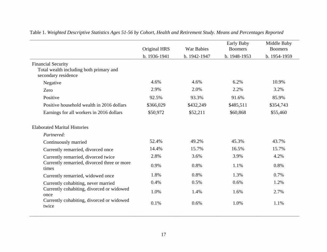
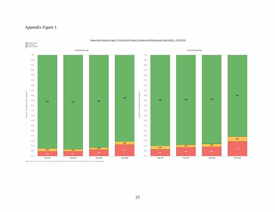
Table 1 presents weighted descriptive statistics for financial, marital history, and other

measures by cohort. Looking first at the results for wealth we see that the rate of negative wealth

holdings has increased substantially from 5 percent to 11 percent when comparing the original

HRS cohort, born between 1936 and 1941, and the Middle Baby Boom cohort, born between

1954 and 1959. This sizable increase in negative wealth may foreshadow financial trouble in the

coming years for more recently born cohorts given the age group in question—ages 51 to 56—

are often at near peak levels of wealth accrual and will likely face declining rates of wealth as

savings are depleted to meet retirement and health costs associated with aging. Rates of zero

wealth, reflecting those who are staying afloat financially but have no wealth cushion to absorb

future shocks, has remained fairly stable over the 20-year period. And as a corollary to the rise

in negative wealth, we see declines in positive wealth from 93 percent to 86 percent over this

period. When considering the loss in overall household wealth over the four cohorts, it is

instructive to see how this translates to real dollars, adjusted to 2016 levels. When the original

HRS cohort reached ages 51-56, their average positive household wealth was $366,029. This

rose steadily for the next two cohorts reaching middle age, to $432,249 among War Babies, and

$485,511 among Early Baby Boomers. The first decline in wealth over three cohorts was seen

among the Baby Boomers, who fell below the baseline levels to $354,743 indicating a real

decline in wealth between those born in 1936-41 and those born in 1954-59. Taken together, the

two wealth-related findings suggest that both the number of people with positive wealth has been

declining, and further, among those who report positive wealth, the actual amount of wealth

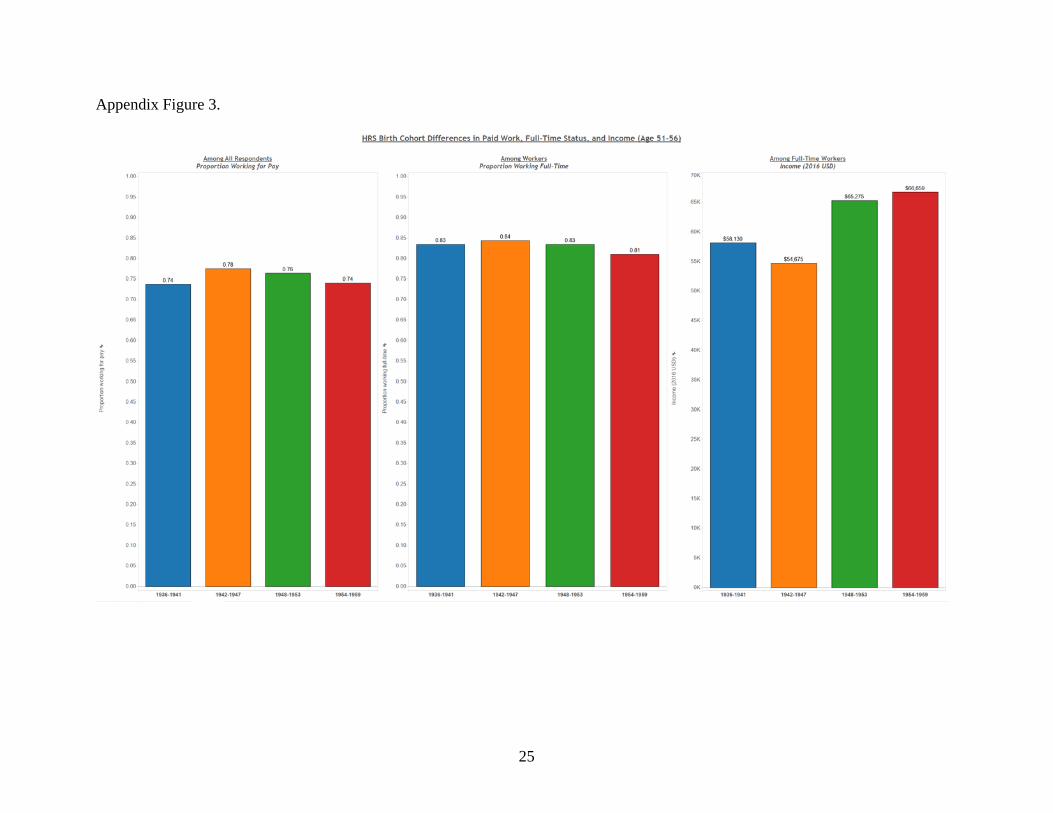
accrual is also declining. The pattern is slightly less bleak when income is considered. Here we

see that the average income (adjusted to 2016 dollars) was $50,972 for the original HRS cohort,

which rose slightly for War Babies to $52,211, and then again for Early Baby Boomers to

$60,868, and then fell for Middle Baby Boomers to $55,460. While the decline in earned income

is notable, the losses were not as extreme as those reported for wealth, as there was still a rise in

income since the baseline measure. We evaluate the statistical significance of cohort differences

in financial measures in our multivariate regression models reported below.

9

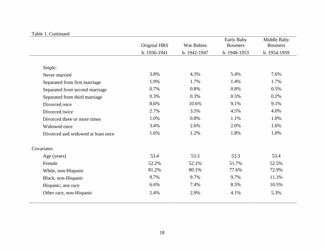
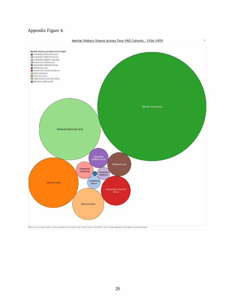
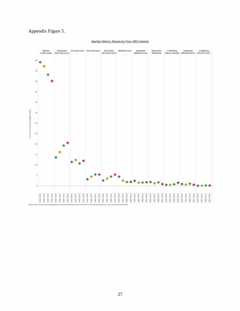
Turning to marital histories, we see that the most common sequence of relationships is

continuously married. However, across cohorts we see a steady decline in the percentage of

those who are continuously married—52 percent among members of the original HRS cohort, 49

percent among War Babies, 45 percent among Early Baby Boomers, and 44 percent among

Middle Baby Boomers. Relatedly, there has been a steady increase in the percentage of adults

who were never married, rising from 4 percent among the HRS cohort to 8 percent among the

Middle Baby Boom cohort. There have also been increases in the amount and type of various

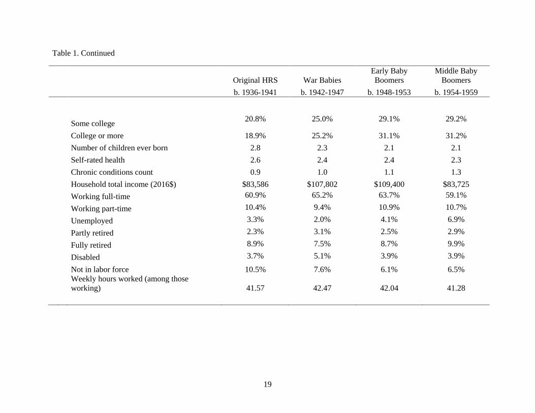
cohabiting relationships. In terms of our covariates, the proportion that is female is nearly

constant across cohorts. A greater share of more recent cohorts are people of color, as well as

people with at least some college education. In addition, members of more recent cohorts

are also more likely to be unemployed and report more comorbidities on average. There have

also been declines in overall fertility levels and self-rated health and increases in the number of

chronic conditions.

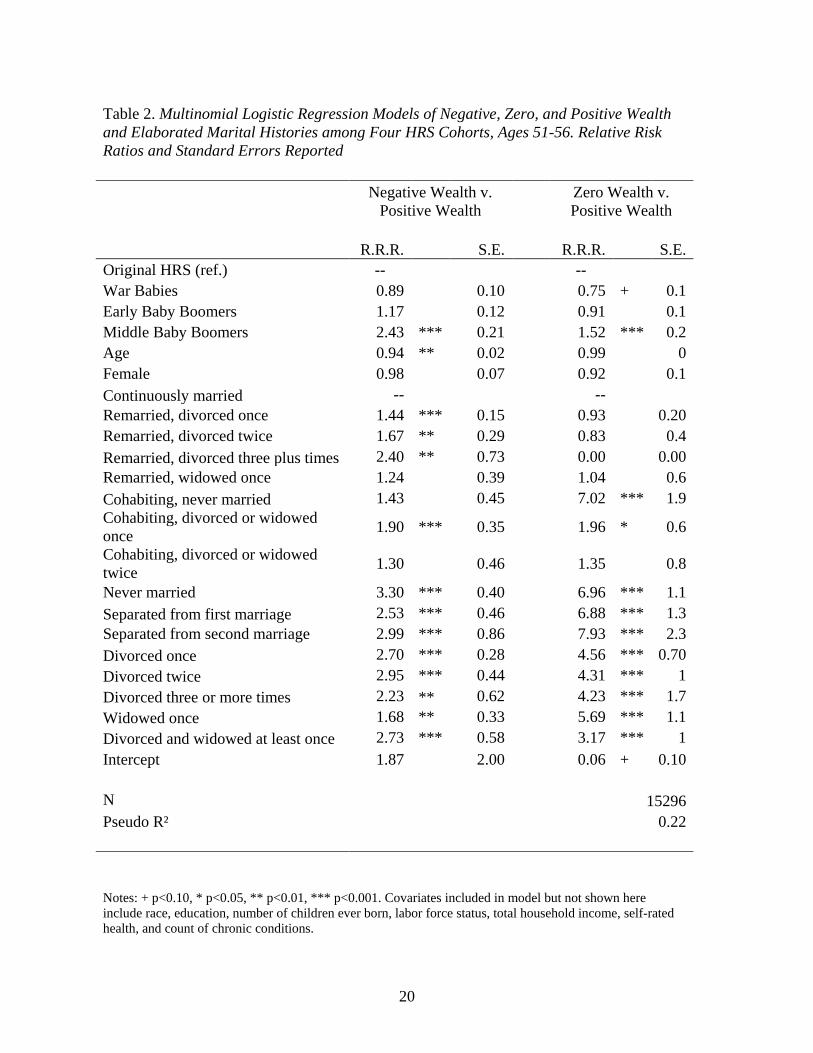
Moving beyond descriptive associations, we assess multivariate models to disentangle the

nature of the relationship between marital history and financial wellbeing, net of controls. First,

we consider wealth. Table 2 presents multinomial logistic regression models of negative and

zero wealth relative to positive wealth. Compared with members of the original HRS cohort,

Middle Baby Boomers are at significantly greater risk of having both negative wealth (2.4 times

greater risk) and zero wealth (1.5 times greater risk). When focusing on negative wealth, we see

that compared with the continuously married, nearly every other marital history pattern is

associated with a greater relative risk of being in the negative wealth category compared to

positive wealth. Most strikingly, those who never married are at 3.3 times greater risk of

experiencing negative wealth compared to continuously married individuals, and those who are

currently single (either through a separation from marriage or after finalizing the divorce) have

between a 2.2 and 3.0 greater risk of experiencing negative wealth than their counterparts who

stayed married. As anticipated by prior research, widowhood was associated with a significantly

increased risk of negative wealth, but this risk was lower than individuals who exited marriage

via divorce or separation. Note that the relationship between marital status and negative wealth

depends on which relationship was being dissolved, with higher risk levels associated with those

in second and third order relationships. For example, the risk of negative wealth was greatest for

those who remarried after three divorces, followed by those remarrying after two divorces, and

10

then those remarrying after one divorce. Similarly, there were rising levels of risk of negative

wealth for those separated from their first and then second marriage and for those who

experienced a first relative to second divorce. We see similar patterns of associations for zero

wealth, although the size of effects were often greater for zero wealth versus positive wealth

compared with negative wealth versus positive wealth. One noteworthy finding from this model

is that adults who cohabit but never marry had seven times the risk of having zero wealth

compared to continuously married respondents. There was no significant effect for this group on

negative wealth, which suggests that while cohabiters continue to have distinctly poorer financial

outcomes than continuously married individuals, these effects appear to be tied to a lack of

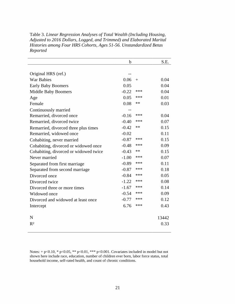
financial growth rather than debt. Table 3 presents ordinary least squares regression models of

logged positive wealth, which accounts for one-third of the total variation in wealth for our

sample (r2 = .33). Compared with members of the original HRS cohort, Middle Baby Boomers

have significantly lower levels of positive wealth. As with models examining negative, zero, and

positive wealth, nearly every marital history pattern has less wealth than the continuously

married, and generally follows the pattern that the number of cumulative disruptions (proxied

here as the higher order status of the relationship being disrupted) is inversely related to overall

wealth.

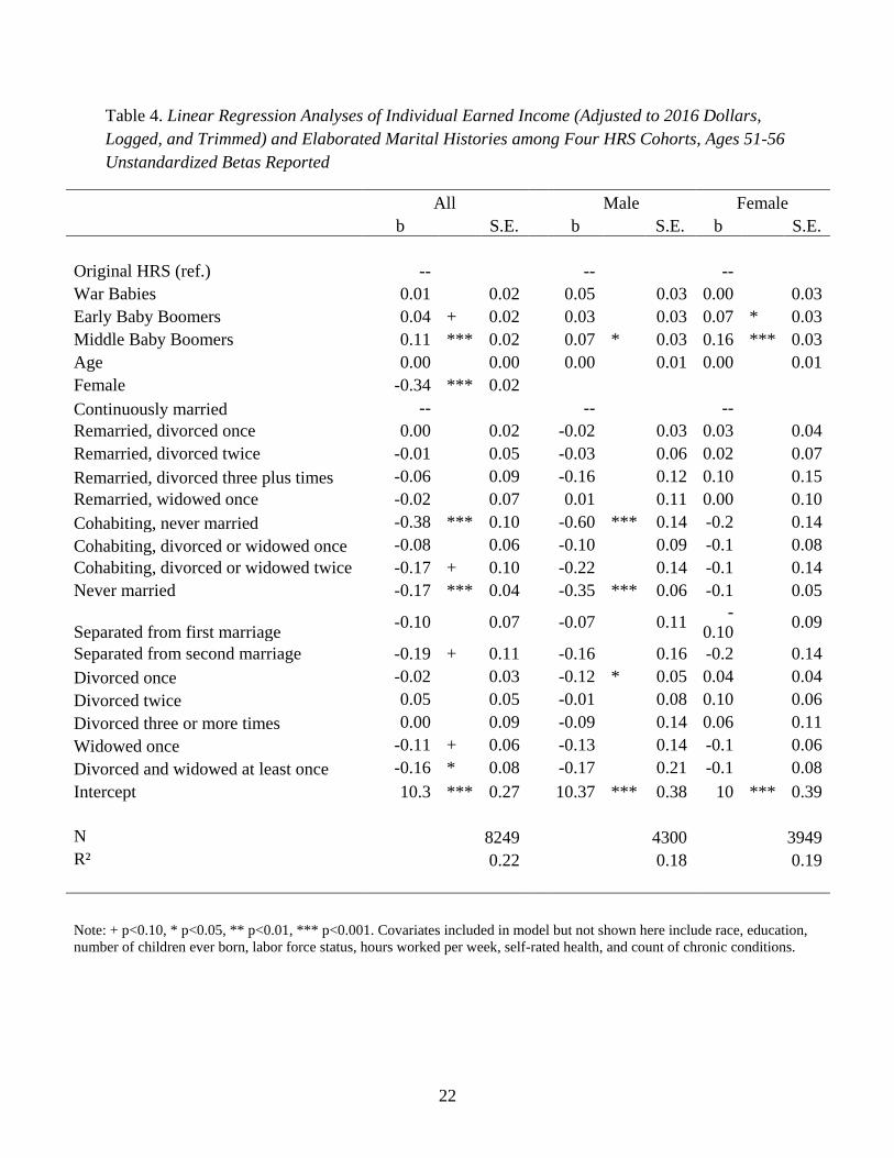
Table 4 presents ordinary least squares regression models of logged positive earnings

among full-time workers, which account for 22 percent of the variation in earnings among our

sample. While gender-cohort interactions were not statistically significant for wealth outcomes,

a gender-cohort interaction was statistically significant for earnings. As such, we present both

pooled results and gender-stratified results. In the pooled model, we observe an increase in

earnings in real terms between members of the original HRS cohort and Middle Baby Boomers.

Gender-stratified models suggest that while both male and female Middle Baby Boomers

experienced increases in earnings, the increase was much larger for women, confirming the

literature on increasing economic parity between the genders. Compared with wealth models,

we find that several marital history patterns are on par with the continuously married in terms of

earnings in both pooled models and models only including men. We take this finding to suggest

that the experience of marital instability may have larger impacts on long-term financial well-

being (assessed here as wealth) and less influence on immediate financial success (assessed here

as income). Notably, for women, we do not observe any significant variation in earnings by

11

marital history once cohort and a rich set of controls were included. This finding is somewhat

surprising given the literature suggesting that women are less likely than men to achieve

affluence without getting and staying married. If this is the case, it does not appear to be

driven—in our data at least—by sustained increases in earnings. Alternately, men do see a

significant improvement in wealth for being continuously married relative to never married

(either staying single or only cohabiting).

Discussion

The Middle Baby Boomers born in the mid-to-late 1950s differ from older cohorts (i.e.

those born in the mid-to-late 1930s) by both marital history and financial security measures.

Middle Baby Boomers are more likely to have negative wealth (i.e. debt) or zero wealth, and

those who have positive wealth have lower levels of wealth, suggesting that in terms of

household wealth and savings, they are the least prepared for retirement of the last four

generations. On the other hand, after controlling for education, race, and health, Middle Baby

Boomers working full-time have higher earnings than earlier cohorts, especially among women,

which may counteract some of the negative effects of wealth. One explanation for these findings

is the increase in martial instability experienced by Middle Baby Boomers. Increasing marital

instability as well as other social, economic, and cultural factors may have encouraged labor

force participation and strengthened attachment, resulting in higher real earnings. However,

increasing marital instability remains detrimental to wealth accumulation.

As seen in multivariate models of household wealth and individual income, marital

history has an important role to play in understanding the financial well-being of pre-retirees

over the last twenty years. More recent cohorts are less likely to be continuously married than

previous cohorts, and this distinction is associated with significant declines in wealth overall and

with significant declines in income for men. A key finding from our study is that the relationship

between marital history and financial security depends on whether wealth or earnings is

examined. Specifically, the economic benefits of continuous marriage are more pronounced for

wealth than earnings, and we believe this may stem from the long-term accrual of advantage

linking marriage to wealth that is less apparent in the more immediate (and less significant)

impact of marriage on earnings. Our findings that remarriage is significantly associated with

lower wealth suggests that the wealth advantage to continuous marriage is not due to the

12

presence of two partners alone. Given that more recent cohorts are less likely to have access

defined benefit plans, as well as the related increasing emphasis on individuals rather than

employers to navigate the risks of retirement planning (Harrington Meyer and Herd 2007,

Poterba 2014), our findings highlight the importance of understanding that individuals’ own

financial resources are more important than ever for retirement income policy. Further, our

findings suggest that increasing relationship uncertainty tied to rising marital history complexity

may be intertwined with financial uncertainty and vulnerability.

There are important limitations of this work. First, while our elaborated marital histories

measures provide considerably greater detail than most previous studies, even these detailed

categories obscure important variation. For example, the never-married group likely contains

particularly economically advantaged women (such as those who privileged their careers over

marriage and children) and particularly economically disadvantaged women (such as never-

married single mothers). Due to statistical power limitations, we were unable to jointly capture

fertility and marital histories, which includes the growing phenomenon of multi-partnered

fertility (Dorius 2012). Second, our analysis of positive wealth and earnings levels likely

obscures important variation in the role of marital histories across the wealth and income

distribution. Previous studies, for example, have documented important variation across the

wealth distribution in terms of racial inequality (e.g. Addo and Lichter 2013, Killewald 2013).

Likewise our focus on average wealth and earnings rather than the entire distribution of these

facets of financial security may understate the full role of marital histories in the economic

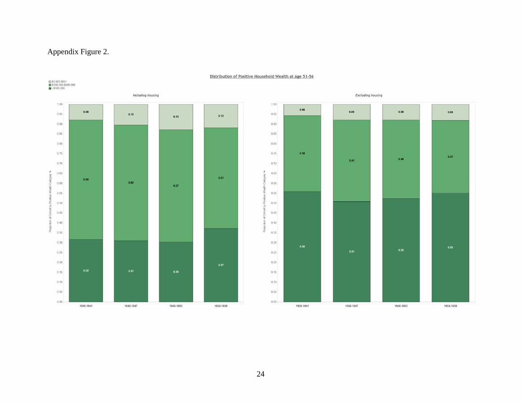
prospects of older Americans. And third, we use the most inclusive definition of household

wealth available in the HRS—one that includes housing wealth. Because a large share of many

older individuals’ wealth is in real property, the inclusion of housing presents a rosier picture of

wealth profiles compared to wealth measures that are restricted to comparatively liquid assets

such as savings accounts and stock portfolios (see Appendix Figure 1).

In addition, while the examination of different cohorts at the same ages enables us to

assess cohort variation in financial security, our approach cannot isolate period effects. The most

serious of these is the measurement of assets for Middle Baby Boomers following the Great

Recession of 2007-2009. Prior work documents the myriad economic ramifications of the

economic downturn for older Americans (Gustman, Steinmeier, and Tabatabai 2012, Johnson

2012, Munnell and Rutledge 2013). To some extent, the wealth of Middle Baby Boomers may

13

have rebounded since our 2010 measures, resulting in a (temporary) understatement of assets in

our data. However, our findings of a higher proportion of Middle Baby Boomers with negative

or zero wealth suggests that this cohort is indeed less prepared for retirement than earlier cohorts.

A final limitation of the present study is that, as in other studies, there is substantial missing data

on economic measures in the HRS. The HRS’ use of bracket unfolding techniques, along with

RAND-provided income and wealth imputations, help to mitigate this drawback.

The present study suggests several fruitful directions for future research. As noted

among limitations, additional detail in marital histories may yield further insights into the

economic fates of recent cohorts in retirement. Work with the National Longitudinal Survey of

Youth examining Middle Baby Boomers observes over 600 marital and relationship patterns.2 In

addition, though we examine three distinct and important dimensions of financial security—the

presence of negative, zero, or positive household wealth; absolute levels of household wealth;

and absolute levels of earnings—future work should explore the relationship between marital

histories and additional dimensions of financial well-being, such as access to defined-benefit

pension plans, Social Security income and wealth projections, and poverty. Finally, given the

strong relationship between marriage and health across the life course (Hughes and Waite 2009,

Waite 1995), the increasing complexity of marital histories may also have implications for the

health of more recent cohorts entering later life. As more recent cohorts spend less time in first

marriages, and experience more dissolution in later life (Brown and Lin 2012), these individuals

may enter later life with more chronic conditions and disability, with potential implications for

Social Security, Medicare, and Medicaid expenditures.

Conclusion

Using data from four cohorts of men and women from the HRS, we examined the

relationship between detailed marital histories and three dimensions of financial security: the

presence of negative, zero, or positive wealth; positive levels of household wealth; and positive

levels of earnings. We found that Middle Baby Boomers were more likely to have negative

wealth (i.e. debt) and zero wealth compared with members of the original HRS cohort at the

same ages (51-56), and among those with positive wealth, had lower levels. In addition,

unemployment levels were higher among Middle Baby Boomers than previous cohorts at the

2 Authors’ calculations.

14

same ages. However, the economic news is not all bad, as baby boomers working full time had

higher real earnings compared with their original HRS counterparts. We also found that more

recent cohorts are less likely to be continuously married and more likely to be never married,

both of which are negatively associated with financial wellbeing in pre-retirement. Based on

these findings, we suggest two policy implications. First, Social Security policy changes might

consider the increasing heterogeneity in marital histories and changing economic circumstances

of more-recent cohorts approaching retirement. The increasing complexity of the marital

histories of Middle Baby Boomers may be a harbinger of even greater family diversity for

cohorts to come (i.e. Millennials). Further, more recent cohorts may also enter late mid-life with

even less wealth than Middle Baby Boomers due to the stagnant economic conditions of the

Great Recession and high levels of student debt. These economic conditions relatively early in

adulthood may not only impede wealth accumulation but also family formation (Addo 2014),

which may have long-ranging consequences across the life course. Second, greater attention can

be paid to two growing segments of adults in late mid-life: those with zero wealth and those in

debt, who are approaching retirement in a particularly precarious position. Such individuals are

more likely to rely on Social Security in the future and thus may be particularly adversely

affected if proposed cuts to Social Security retirement benefits were enacted.

15

References Addo, Fenaba R. 2014. “Debt, Cohabitation, and Marriage in Young Adulthood.”

Demography 51(5): 1677-1701. Addo, Fenaba R. and Daniel T. Lichter. 2013. “Marriage, Marital History, and Black–White

Wealth Differentials among Older Women.” Journal of Marriage and Family 75(2): 342-362.

Brown, Susan L. and I-Fen Lin. 2012. “The Gray Divorce Revolution: Rising Divorce among

Middle-Aged and Older Adults, 1990–2010.” The Journals of Gerontology Series B: Psychological Sciences and Social Sciences 67(6): 731-741.

Bureau of Labor Statistics. 2016. Databases, Tables & Calculators by Subject: CPI Inflation

Calculator. Last retrieved May 5, 2016: http://www.bls.gov/data/inflation_calculator.htm. Cherlin, Andrew J. 2010. “Demographic Trends in the United States: A Review of Research in

the 2000s.” Journal of Marriage and Family 72(3): 403-419. Collins, J. Michael, John Karl Scholz, and Ananth Seshadri. 2013. “The Assets and Liabilities of

Cohorts: The Antecedents of Retirement Security.” Research Paper 2013-296. Ann Arbor: MI: Michigan Retirement Research Center.

Dorius, Cassandra. 2012. “New Approaches to Measuring Multipartnered Fertility over the Life Course.” PSC Research Report No. 12-769: www.psc.isr.umich.edu/pubs/pdf/rr12-769.pdf.

Gustman, Alan L., Thomas L. Steinmeier, and Nahid Tabatabai. 2012. “How Did the Recession

of 2007-2009 Affect the Wealth and Retirement of the Near Retirement Age Population in the Health and Retirement Study?” Social Security Bulletin 72(4): 47-65.

Harrington Meyer, Madonna and Pamela Herd. 2007. Market Friendly or Family Friendly? The

State and Gender Inequality in Old Age: The State and Gender Inequality in Old Age. New York, NY: Russell Sage Foundation.

Hirschl, Thomas A., Joyce Altobelli, and Mark R. Rank. 2003. “Does Marriage Increase the

Odds of Affluence? Exploring the Life Course Probabilities.” Journal of Marriage and Family 65(4): 927-938.

Holden, Karen C. and Pamela J. Smock. 1991. “The Economic Costs of Marital Dissolution:

Why Do Women Bear a Disproportionate Cost?” Annual Review of Sociology 17: 51-78. Hughes, Mary Elizabeth and Linda J. Waite. 2009. “Marital Biography and Health at Mid-

Life.” Journal of Health and Social Behavior 50(3): 344-358.

16

Hurd, Michael D., Erik Meijer, Michael Moldoff, and Susann Rohwedder. Forthcoming. “Improved Wealth Measures in the Health and Retirement Study: Asset Reconciliation and Cross-Wave Imputation.” Santa Monica, CA: RAND Corporation.

Johnson, Richard W. 2012. “Older Workers, Retirement, and the Great Recession.” New York,

NY: Russell Sage Foundation. Johnson, Richard W. and Melissa M. Favreault. 2004. “Economic Status in Later Life among

Women Who Raised Children Outside of Marriage.” The Journals of Gerontology Series B: Psychological Sciences and Social Sciences 59(6): S315-S323.

Killewald, Alexandra. 2013. “Return to Being Black, Living in the Red: A Race Gap in Wealth

That Goes Beyond Social Origins.” Demography 50(4): 1177-1195. Lee, Ronald, Sang-Hyop Lee, and Andrew Mason. 2006. “Charting the Economic Life Cycle.”

Working Paper 12379. Cambridge, MA: National Bureau of Economic Research. Munnell, Alicia H. and Matthew S. Rutledge. 2013. “The Effects of the Great Recession on the

Retirement Security of Older Workers.” The ANNALS of the American Academy of Political and Social Science 650(1): 124-142.

Poterba, James M. 2014. “Retirement Security in an Aging Population.” The American Economic

Review 104(5): 1-30. Waite, Linda J. 1995. “Does Marriage Matter?” Demography 32(4): 483-507. Wilmoth, Janet and Gregor Koso. 2002. “Does Marital History Matter? Marital Status and

Wealth Outcomes among Preretirement Adults.” Journal of Marriage and Family 64(1): 254-268.

17

Table 1. Weighted Descriptive Statistics Ages 51-56 by Cohort, Health and Retirement Study. Means and Percentages Reported

Original HRS War Babies Early Baby Boomers

Middle Baby Boomers

b. 1936-1941 b. 1942-1947 b. 1948-1953 b. 1954-1959 Financial Security

Total wealth including both primary and secondary residence

Negative 4.6% 4.6% 6.2% 10.9%

Zero 2.9% 2.0% 2.2% 3.2%

Positive 92.5% 93.3% 91.6% 85.9% Positive household wealth in 2016 dollars $366,029 $432,249 $485,511 $354,743 Earnings for all workers in 2016 dollars $50,972 $52,211 $60,868 $55,460 Elaborated Marital Histories Partnered: Continuously married 52.4% 49.2% 45.3% 43.7% Currently remarried, divorced once 14.4% 15.7% 16.5% 15.7% Currently remarried, divorced twice 2.8% 3.6% 3.9% 4.2%

Currently remarried, divorced three or more times 0.9% 0.8% 1.1% 0.8%

Currently remarried, widowed once 1.8% 0.8% 1.3% 0.7% Currently cohabiting, never married 0.4% 0.5% 0.6% 1.2%

Currently cohabiting, divorced or widowed once 1.0% 1.4% 1.6% 2.7%

Currently cohabiting, divorced or widowed twice 0.1% 0.6% 1.0% 1.1%

18

Table 1. Continued

Original HRS War Babies

Early Baby Boomers

Middle Baby Boomers

b. 1936-1941 b. 1942-1947 b. 1948-1953 b. 1954-1959 Single: Never married 3.8% 4.3% 5.4% 7.6% Separated from first marriage 1.9% 1.7% 1.4% 1.7% Separated from second marriage 0.7% 0.8% 0.8% 0.5% Separated from third marriage 0.3% 0.3% 0.5% 0.2% Divorced once 8.6% 10.6% 9.1% 9.1% Divorced twice 2.7% 3.5% 4.5% 4.0% Divorced three or more times 1.0% 0.8% 1.1% 1.0% Widowed once 3.4% 2.6% 2.0% 1.6% Divorced and widowed at least once 1.6% 1.2% 1.8% 1.0%

Covariates Age (years) 53.4 53.3 53.3 53.4 Female 52.2% 52.1% 51.7% 52.5% White, non-Hispanic 81.2% 80.1% 77.6% 72.9%

Black, non-Hispanic 9.7% 9.7% 9.7% 11.3%

Hispanic, any race 6.6% 7.4% 8.5% 10.5%

Other race, non-Hispanic 2.4% 2.9% 4.1% 5.3%

19

Table 1. Continued

Original HRS War Babies Early Baby Boomers

Middle Baby Boomers

b. 1936-1941 b. 1942-1947 b. 1948-1953 b. 1954-1959 Some college 20.8% 25.0% 29.1% 29.2%

College or more 18.9% 25.2% 31.1% 31.2% Number of children ever born 2.8 2.3 2.1 2.1 Self-rated health 2.6 2.4 2.4 2.3 Chronic conditions count 0.9 1.0 1.1 1.3 Household total income (2016$) $83,586 $107,802 $109,400 $83,725 Working full-time 60.9% 65.2% 63.7% 59.1%

Working part-time 10.4% 9.4% 10.9% 10.7%

Unemployed 3.3% 2.0% 4.1% 6.9%

Partly retired 2.3% 3.1% 2.5% 2.9%

Fully retired 8.9% 7.5% 8.7% 9.9%

Disabled 3.7% 5.1% 3.9% 3.9%

Not in labor force 10.5% 7.6% 6.1% 6.5%

Weekly hours worked (among those working) 41.57 42.47 42.04 41.28

20

Table 2. Multinomial Logistic Regression Models of Negative, Zero, and Positive Wealth and Elaborated Marital Histories among Four HRS Cohorts, Ages 51-56. Relative Risk Ratios and Standard Errors Reported

Negative Wealth v.

Positive Wealth Zero Wealth v. Positive Wealth

R.R.R. S.E. R.R.R. S.E.

Original HRS (ref.) -- -- War Babies 0.89 0.10 0.75 + 0.1 Early Baby Boomers 1.17 0.12 0.91 0.1 Middle Baby Boomers 2.43 *** 0.21 1.52 *** 0.2 Age 0.94 ** 0.02 0.99 0 Female 0.98 0.07 0.92 0.1 Continuously married -- -- Remarried, divorced once 1.44 *** 0.15 0.93 0.20 Remarried, divorced twice 1.67 ** 0.29 0.83 0.4 Remarried, divorced three plus times 2.40 ** 0.73 0.00 0.00 Remarried, widowed once 1.24 0.39 1.04 0.6 Cohabiting, never married 1.43 0.45 7.02 *** 1.9 Cohabiting, divorced or widowed once 1.90 *** 0.35 1.96 * 0.6

Cohabiting, divorced or widowed twice 1.30 0.46 1.35 0.8

Never married 3.30 *** 0.40 6.96 *** 1.1 Separated from first marriage 2.53 *** 0.46 6.88 *** 1.3 Separated from second marriage 2.99 *** 0.86 7.93 *** 2.3 Divorced once 2.70 *** 0.28 4.56 *** 0.70 Divorced twice 2.95 *** 0.44 4.31 *** 1 Divorced three or more times 2.23 ** 0.62 4.23 *** 1.7 Widowed once 1.68 ** 0.33 5.69 *** 1.1 Divorced and widowed at least once 2.73 *** 0.58 3.17 *** 1 Intercept 1.87 2.00 0.06 + 0.10 N 15296 Pseudo R² 0.22

Notes: + p<0.10, * p<0.05, ** p<0.01, *** p<0.001. Covariates included in model but not shown here include race, education, number of children ever born, labor force status, total household income, self-rated health, and count of chronic conditions.

21

Table 3. Linear Regression Analyses of Total Wealth (Including Housing, Adjusted to 2016 Dollars, Logged, and Trimmed) and Elaborated Marital Histories among Four HRS Cohorts, Ages 51-56. Unstandardized Betas Reported b S.E. Original HRS (ref.) -- War Babies 0.06 + 0.04 Early Baby Boomers 0.05 0.04 Middle Baby Boomers -0.22 *** 0.04 Age 0.05 *** 0.01 Female 0.08 ** 0.03 Continuously married -- Remarried, divorced once -0.16 *** 0.04 Remarried, divorced twice -0.40 *** 0.07 Remarried, divorced three plus times -0.42 ** 0.15 Remarried, widowed once -0.02 0.11 Cohabiting, never married -0.87 *** 0.15 Cohabiting, divorced or widowed once -0.48 *** 0.09 Cohabiting, divorced or widowed twice -0.43 ** 0.15 Never married -1.00 *** 0.07 Separated from first marriage -0.89 *** 0.11 Separated from second marriage -0.87 *** 0.18 Divorced once -0.84 *** 0.05 Divorced twice -1.22 *** 0.08 Divorced three or more times -1.67 *** 0.14 Widowed once -0.54 *** 0.09 Divorced and widowed at least once -0.77 *** 0.12 Intercept 6.76 *** 0.43 N 13442 R² 0.33

Notes: + p<0.10, * p<0.05, ** p<0.01, *** p<0.001. Covariates included in model but not shown here include race, education, number of children ever born, labor force status, total household income, self-rated health, and count of chronic conditions.

22

Table 4. Linear Regression Analyses of Individual Earned Income (Adjusted to 2016 Dollars, Logged, and Trimmed) and Elaborated Marital Histories among Four HRS Cohorts, Ages 51-56 Unstandardized Betas Reported

All Male Female b S.E. b S.E. b S.E. Original HRS (ref.) -- -- -- War Babies 0.01 0.02 0.05 0.03 0.00 0.03 Early Baby Boomers 0.04 + 0.02 0.03 0.03 0.07 * 0.03 Middle Baby Boomers 0.11 *** 0.02 0.07 * 0.03 0.16 *** 0.03 Age 0.00 0.00 0.00 0.01 0.00 0.01 Female -0.34 *** 0.02 Continuously married -- -- -- Remarried, divorced once 0.00 0.02 -0.02 0.03 0.03 0.04 Remarried, divorced twice -0.01 0.05 -0.03 0.06 0.02 0.07 Remarried, divorced three plus times -0.06 0.09 -0.16 0.12 0.10 0.15 Remarried, widowed once -0.02 0.07 0.01 0.11 0.00 0.10 Cohabiting, never married -0.38 *** 0.10 -0.60 *** 0.14 -0.2 0.14 Cohabiting, divorced or widowed once -0.08 0.06 -0.10 0.09 -0.1 0.08 Cohabiting, divorced or widowed twice -0.17 + 0.10 -0.22 0.14 -0.1 0.14 Never married -0.17 *** 0.04 -0.35 *** 0.06 -0.1 0.05

Separated from first marriage -0.10 0.07 -0.07 0.11 -0.10 0.09

Separated from second marriage -0.19 + 0.11 -0.16 0.16 -0.2 0.14 Divorced once -0.02 0.03 -0.12 * 0.05 0.04 0.04 Divorced twice 0.05 0.05 -0.01 0.08 0.10 0.06 Divorced three or more times 0.00 0.09 -0.09 0.14 0.06 0.11 Widowed once -0.11 + 0.06 -0.13 0.14 -0.1 0.06 Divorced and widowed at least once -0.16 * 0.08 -0.17 0.21 -0.1 0.08 Intercept 10.3 *** 0.27 10.37 *** 0.38 10 *** 0.39 N 8249 4300 3949 R² 0.22 0.18 0.19

Note: + p<0.10, * p<0.05, ** p<0.01, *** p<0.001. Covariates included in model but not shown here include race, education, number of children ever born, labor force status, hours worked per week, self-rated health, and count of chronic conditions.

23

Appendix Figure 1.

24

Appendix Figure 2.

25

Appendix Figure 3.

26

Appendix Figure 4.

27

Appendix Figure 5.

28

RECENT WORKING PAPERS FROM THE CENTER FOR RETIREMENT RESEARCH AT BOSTON COLLEGE

Pension Participation, Wealth, and Income: 1992-2010 Alicia H. Munnell, Wenliang Hou, Anthony Webb, and Yinji Li, July 2016 The Interconnected Relationships of Health Insurance, Health, and Labor Market Outcomes Matthew S. Rutledge, July 2016 Labor Force Dynamics in the Great Recession and Its Aftermath: Implications for Older Workers Gary Burtless, July 2016 Elderly Poverty in the United States in the 21st Century: Exploring the Role of Assets in the Supplemental Poverty Measure Christopher Wimer and Lucas Manfield, November 2015 The Economic Burden of Out-of-Pocket Medical Expenditures Before and After Implementation of the Medicare Prescription Drug Program Ayse Akincigil and Karen Zurlo, November 2015 The Impact of Temporary Assistance Programs on the Social Security Claiming Age Geoffrey T. Sanzenbacher, April Yanyuan Wu, and Matthew S. Rutledge, October 2015 Do Households Increase Their Savings When the Kids Leave Home? Irena Dushi, Alicia H. Munnell, Geoffrey T. Sanzenbacher, and Anthony Webb, September 2015 Evaluating the Impact of Social Security Benefits on Health Outcomes Among the Elderly Padmaja Ayyagari, September 2015 Does Age-Related Decline in Ability Correspond with Retirement Age? Anek Belbase, Geoffrey T. Sanzenbacher, and Christopher M. Gillis, September 2015 Job Polarization and Labor Market Outcomes for Older, Middle-Skilled Workers Matthew S. Rutledge and Qi Guan, September 2015 What Causes Workers to Retire Before They Plan? Alicia H. Munnell, Geoffrey T. Sanzenbacher, and Matthew S. Rutledge, September 2015 Calculating Neutral Increases in Retirement Age by Socioeconomic Status Geoffrey T. Sanzenbacher, Anthony Webb, Candace M. Cosgrove, and Natalia S. Orlova, August 2015

All working papers are available on the Center for Retirement Research website (http://crr.bc.edu) and can be requested by e-mail (crr@bc.edu) or phone (617-552-1762).