Embed Size (px)
Citation preview

Marital Disruption and Economic Well-being:
A Comparative Analysis
Arnstein Aassve - Gianni Betti - Stefano Mazzuco - Letizia Mencarini
ISER Working Paper 2006-07
Institute for Social and Economic Research The Institute for Social and Economic Research (ISER) specialises in the production and analysis of longitudinal data. ISER incorporates the following centres:
• ESRC Research Centre on Micro-social Change. Established in 1989 to identify, explain, model
and forecast social change in Britain at the individual and household level, the Centre specialises in research using longitudinal data.
• ESRC UK Longitudinal Studies Centre. A national resource centre for promoting longitudinal
research and for the design, management and support of longitudinal surveys. It was established by the ESRC as independent centre in 1999. It has responsibility for the British Household Panel Survey (BHPS).
• European Centre for Analysis in the Social Sciences. ECASS is an interdisciplinary research
centre which hosts major research programmes and helps researchers from the EU gain access to longitudinal data and cross-national datasets from all over Europe.
The British Household Panel Survey is one of the main instruments for measuring social change in Britain. The BHPS comprises a nationally representative sample of around 9,000 households and over 16,000 individuals who are reinterviewed each year. The questionnaire includes a constant core of items accompanied by a variable component in order to provide for the collection of initial conditions data and to allow for the subsequent inclusion of emerging research and policy concerns. Among the main projects in ISER’s research programme are: the labour market and the division of domestic responsibilities; changes in families and households; modelling households’ labour force behaviour; wealth, well-being and socio-economic structure; resource distribution in the household; and modelling techniques and survey methodology. BHPS data provide the academic community, policymakers and private sector with a unique national resource and allow for comparative research with similar studies in Europe, the United States and Canada. BHPS data are available from the UK Data Archive at the University of Essex http://www.data-archive.ac.uk Further information about the BHPS and other longitudinal surveys can be obtained by telephoning +44 (0) 1206 873543. The support of both the Economic and Social Research Council (ESRC) and the University of Essex is
gratefully acknowledged. The work reported in this paper is part of the scientific programme of the
Institute for Social and Economic Research.

Readers wishing to cite this document are asked to use the following form of words:
Aassve, A., Betti, G., Mazzuco, S. and Mencarini, L. (March 2006) ‘Marital Disruption and Economic Well-being: A Comparative Analysis’, ISER Working Paper 2006-07. Colchester: University of Essex.
For an on-line version of this working paper and others in the series, please visit the Institute’s website at: http://www.iser.essex.ac.uk/pubs/workpaps/
Institute for Social and Economic Research University of Essex Wivenhoe Park Colchester Essex CO4 3SQ UK Telephone: +44 (0) 1206 872957 Fax: +44 (0) 1206 873151 E-mail: [email protected] Website: http://www.iser.essex.ac.uk
© March 2006 All rights reserved. No part of this publication may be reproduced, stored in a retrieval system or transmitted, in any form, or by any means, mechanical, photocopying, recording or otherwise, without the prior permission of the Communications Manager, Institute for Social and Economic Research.
ABSTRACT
Though there is a considerable literature concerned with the economic consequences of
marital breakdown, there is still substantial disagreement in terms of its magnitude. One of
the major problems underlying this debate is how economic well-being is defined. In this
work we implement several measures of well-being of monetary and multidimensional nature
using data from European Community Household Panel. Another issue in this literature
concerns selection bias of divorcing couples. We tackle this issue using a propensity score
matching technique combined with a Difference-in-Differences estimator. Results confirm
the importance of well-being definition. We find a high gender bias when using monetary
measures but a considerably lower one or even non existent when using non-monetary
indices.
5
NON-TECHNICAL SUMMARY
The present work is concerned with the economic consequences of marital disruption
for both the members of the separating couples. Most of the literature on this topic assess
whether there is a large gender bias, women being exposed to high poverty risks in the
aftermath of separation whereas men seem not to experience any dramatic drop of their
income and sometimes they can be even better off after divorce/separation. Some authors
(McManus and DiPrete, 2001) challenge this evidence, suggesting that the gender bias is less
strong than what is generally acknowledged, and also men economically suffer after marital
disruption. Here we suggest that two main issues are behind this debate: firstly the
conventional measures of well-being (i.e. income and poverty status) are not entirely
satisfying. Poverty status creates distinction between “poor” and “non poor”, but it is not clear
which poverty line should be considered appropriate and why. Moreover, income and poverty
status do not encapsulate all the dimensions underlying poverty and social exclusion - only
the monetary one. We may expect that men are not suffering in monetary terms in the
aftermath of separation but they experience an increased deprivation in lifestyle standards all
the same because of a rise in expenses due to alimonies payments, new dwelling costs, etc.
The second issue concerns selection. This is driven by the fact that men and women who are
at high risk of entering poverty may be more likely to avoid separation. By using a propensity
score matching procedure combined with a Difference-in-differences estimator we control for
such a selection bias.
We expect that by using different measures of well-being we are able to observe that
both men and women experience an economic deprivation after separation being women more
deprived in monetary terms and men in non monetary terms. The results confirm largely to
our expectations: it is confirmed that the definition of poverty threshold is an important issue.
Results differ considerably depending on whether we use a 50%, a 60%, or 70% poverty line.
Moreover when we use monetary measures (i.e. poverty status and relative income) it is
unquestionable that women suffer a disproportionately larger negative effect than men. Also
important is that by using monetary measures, we find that most of the results are consistent
with welfare regime theory. However, the non-monetary measures (i.e. deprivation indices)
provide a different picture. Women are still found to suffer significantly more than men, but it
is also clear that men's level of deprivation also increases, and in some cases there is no
significant difference between the ATT estimated for men and women (this is case in Liberal
countries when using the overall deprivation index and the secondary lifestyle deprivation
index).
6
Children play an important role in explaining the gender differences. If there are
children in the conjugal dwelling, then mothers are much more likely to be granted custody
following a divorce. Thus the divorce event will for many women imply reduced income
(poorer access to the husband’s income) and a higher relative expenditure. Men are instead
likely to live alone or with parents, and are much less likely to experience poverty and
financial strain. Considering couples with children only in the analysis of entering poverty, we
notice that in Liberal and Mediterranean countries the gender gap is even larger, in
Scandinavian countries is smaller, and in the Conservative countries it remains, more or less
unaltered.
However, in terms of deprivation, men do suffer significantly. Many of the items used
to compute the deprivation index refers to characteristics of the dwelling. If it is the case that
men normally has to leave the dwelling following a divorce, he will in the short run at least,
loose out on many of the goods and services that the household would provide. So though
men are not worse off financially, they are worse off in terms of consumer durables and
certain expenditure goods. It also seems likely that the new dwelling is often of poorer quality
of the original dwelling, which is consistent with our estimates.
The gender difference is clearly smaller when children are not present in the dwelling.
With no children, the effect on lifestyle deprivation among men becomes higher, whereas it is
slightly smaller for women. One important factor here is that it is less clear which of the
spouses that will stay put in the conjugal dwelling if the couple has no children.
7
1. Introduction Household structures across Europe are changing and evolving. A particular feature of
modern family patterns is the significant increase in marital breakdowns. As a result the
number of children living in single parent households, most of which are female-headed, has
also increased. Though the issue of divorce and marital breakdowns is not new in most
countries, it is an issue of continued concern. Most of the debate around the economic
consequences of divorce is focussed on gender inequalities, and the most consistent finding
from the literature is a rather sharp gender difference in terms of financial outcomes following
a marital disruption. Early longitudinal research from the US and Europe showed that women
experiencing a divorce tend to suffer a substantial loss of income, whereas men’s economic
circumstances seem rather unaffected or even improving slightly in some cases (Burkhauser
et al., 1991; Fritzell, 1990; Jarvis and Jenkins, 1999; Manting and Bouman 2004, Poortman,
2000, 2002; Smock 1993, 1994). The reasons behind this pattern are many. One is that
women tend to have lower labour market attachment, and therefore facing lower earnings.
Another reason is that children tend to stay with the mother following a divorce, in many
cases imposing a major strain on the single female-headed household. Finally, lack of state
support is another reason for why many divorced women suffer financially.
An equally consistent finding is strong country differences in terms of the economic
penalty associated with a marital dissolution (Andreß, 2004; Burkhauser et al., 1991; Duncan
and Hoffman, 1985; Finnie, 1993; Fritzell, 1990; Jarvis and Jenkins, 1999; Smock, 1993,
1994; Smock et al., 1999; Poortman, 2000, 2002). The general pattern is that divorced women
in Scandinavian countries, with their generous welfare provision, are much better off than
divorced women in Britain, a country characterised by poorer welfare provision. Andreß et al.
(2004) comparing Belgium, Germany, Italy, Great Britain, and Sweden analysing the three
main providers of individual welfare: 1) the family, 2) the market and 3) the state, shows that
the configuration of these providers to a large extent determines the economic outcome of
marital dissolution. Due to limited welfare provision, they find British mothers to be
particularly vulnerable, being considerably more dependent on the labour market as a means
to maintain a reasonable level of economic self sufficiency. As expected the UK setting is
quite different to Scandinavian countries, but also different with respect to Continental
countries such as Germany. The social democratic welfare is not only generous in terms of
levels, but also provides strong support in terms of extensive childcare infrastructure, a system
which enables Swedish mothers to work full-time to a much greater extent than other
8
European countries, and especially the UK. However, there is no clear consensus on these
findings, especially concerning the issue of gender differences. Many maintain that the gender
bias is overestimated and that the actual trend constitutes an increasing number of men who
are subject to economic strain following separation (McManus and DiPrete, 2001). Indeed,
there are many reasons to believe that also men experience economic problems following
separation: payment of alimonies, the necessity to find another dwelling (usually the conjugal
house is assigned to the woman especially if there are children) may relevantly and negatively
alter the lifestyle of divorced men. Thus it may seem hard to believe that men are better-off
after marital dissolution.
One of the key problems underlying this debate is the definition and measurement of
the rather vague concept of ‘economic well-being’. Many use income or poverty status as an
overall indicator of economic wellbeing, but these measures suffer from many drawbacks.
Poverty status as a measure of wellbeing is criticised because it divides the population into a
simple poor/non poor dichotomy, based on sometimes arbitrarily chosen thresholds (Cheli and
Lemmi, 1995). Of course, the dichotomy is easily overcome by using income as a measure of
economic wellbeing. But this measure is problematic as it is difficult to assess to what extent
an income loss brings about a real drop in living standards, especially in a comparative
perspective. Moreover both income and poverty status are only monetary measures of well-
being whereas it is well recognised that well-being itself has many more dimensions, often
non monetary in nature (Atkinson, 2003; Bourguignon and Chakravarty, 2003). Another
drawback is that poverty status and income depend on the choice of equivalence scale. Given
that a marital breakdown inevitably modifies the household composition, the equivalence
scale becomes of great consequence. But it is not clear which equivalence to use, especially in
comparative analysis. Thus, it is beneficial to consider measures of wellbeing in which the use
of equivalence scales is not imperative.
In this work we present several well-being measures in order assess whether the
estimated impact of a marital breakdown is dependent on the different definition of well-being
itself. Together with conventional poverty status (defined over three poverty thresholds) we
provide a relative income measure that overcomes the poor/non poor dichotomy, and several
deprivation indices that take into account the multidimensional nature of well-being. We
expect that women are more likely to be deprived in monetary terms in the aftermath of
separation given their greater reliance on partner’s income. Separated men experience instead
a dramatic rise in their expenses if they have to pay alimonies and new dwelling costs (this is
particularly the case when the couple has children as the conjugal house is often assigned to
mothers). The use of different measure of well-being should detect both these effects.
9
Another key issue in assessing the role of marital dissolution on economic wellbeing
concerns selection bias. This is driven by the fact that couples experiencing a marital
separation may be qualitatively different from couples not doing so. For example, women
who are strongly dependent on partner’s income might be less likely to separate from them as
they are aware of the strong economic distress they would experience in the case they split
from their partner (Becker, 1991). One way to tackle this issue is to implement a propensity
score matching technique which nets out the impact of separation from the confounding
effects driven by other observed covariates. Obviously, many other unobserved covariates
may influence the estimate of the effect of marital dissolution. As a result we combine the
propensity score matching approach with a Difference-in-Differences estimator as suggested
by Heckman et al. (1998). In this way we control for the effect caused by unobserved
variables, provided these are time-invariant.
The analysis is implemented using data from European Community Household Panel
(ECHP), which offers a unique scope for comparability at the European level. Uunk (2004)
shows that welfare state arrangements tend to influence the economic consequences of
divorce for women. Income-related arrangements alleviate the economic strains most, then
employment-related arrangements. His findings underpins the importance of welfare regimes,
and shows that differences in terms of economic strains associated with divorce, is not simply
an artefact of country differences. Taking advantage of his work we also analyse the
consequence of marital disruption under different welfare regimes, using the well known
country classification of Esping-Andersen (1999). The analysis provides information about
the possible effects of different family policies in European countries, with respect to
consequences associated with marital disruption. Finally we recognise the importance of
presence of children in the couple, so we make separate estimates for couples with children
only. These estimates are compared to the cases where we include couples with and without
children.
The paper is organised as follows: section 2 explains how we measure economic
wellbeing, section 3 give details of data and estimation strategy, section 4 presents the results
and section 5 concludes.
10
2. Well-being definition and measurement 2.1 Measuring well-being: the conventional approach A simple approach in measuring an individual’s well-being is to construct an individual’s
poverty status. This is normally defined over the household’s net equivalised income, and the
poverty threshold is taken as 60 percent of this income level. Poverty is consequently a
relative measure, and a household is deemed poor if the income falls below this threshold.
This measure takes into account the individual’s position in the income distribution relative to
others within his or her own country. Another important feature of this approach is that it
overcomes the fact that countries will differ in terms of per capita incomes and their
purchasing power parity. A drawback, however, is that it is not clear what constitutes an
appropriate poverty threshold. Often 60% of net equivalised household income is chosen, but
many use alternative poverty thresholds of 50 and 70 percent.
When assessing economic well-being, any measure of household income must be
adjusted to reflect the needs of the people living within the household. Larger households
need more income than smaller households to attain the same standard of living; adults have
different needs than children. Additionally, there are economies of scale, meaning (for
example) that two adults can live together more inexpensively than they could if living
separately. Adjustment for household composition is conventionally done by calculating an
equivalence scale, which is a number reflecting the needs of the household, and dividing total
household income by this equivalence scale. We apply the commonly used OECD modified
equivalence scale, which gives a weight of one for the first adult, 0.5 for other adults than the
household head, and 0.3 for children. Two points should be raised in relation to equivalence
scales. First, the use of equivalence scales assumes that household members share their
income equally, which is not necessarily the case in practice (Browning et al., 1994;
Lundberg et al., 1997; McElroy and Horney, 1981). Secondly, poverty statistics are sensitive
to the choice of equivalence scale: for example, scales which weight children more heavily
will generate higher estimates of poverty among families with children (Aassve et al., 2005).
However, it has also been shown that in comparative studies, the actual poverty ranking of
countries tends to be unaffected by the choice of equivalence scale (e.g. de Vos and Zaidi,
2003).
11
2.2 Well-being as a matter of degree: the relative income measure
Dividing the population into a simple dichotomy of “poor” and “non-poor” is clearly
unsatisfactory. An individual’s well-being is not a single attribute that characterises an
individual or household in terms of its presence or absence (Cheli and Lemmi, 1995). Instead
we propose a measure treating poverty as a matter of degree: in principle all individuals are
subject to poverty, but to varying levels (some much more than others). That level, say 1 for
the poorest to 0 for the richest, is determined by the individual's rank in the income
distribution, and the individual's share in the total income received by the population.
There are several advantages of treating poverty in this way. Most important is that it
utilises the whole distribution directly as a measure of economic wellbeing, as opposed to
dividing the population by a dichotomous category, avoiding specification of a poverty line.
Equally important is the potential of this approach in studying poverty (or more generally,
deprivation in multiple dimensions) in the longitudinal context. The conventional approach
measures mobility simply in terms of movements across some designated poverty line, and
does not reflect the actual magnitude of the changes affecting individuals at all points in the
distribution. Consequently, the degree of mobility of persons near to the chosen line tends to
be over-emphasised, while that of persons far from that line largely ignored. Moreover, we
can expect the resulting measures to be more precise. The sampling error of a distribution is
lower than that of a dichotomy with values concentrated at the two end points. We can also
expect the measures to be less sensitive to local irregularities in the income distribution curve,
and to the particular choice of the poverty threshold (Verma and Betti, 2005).
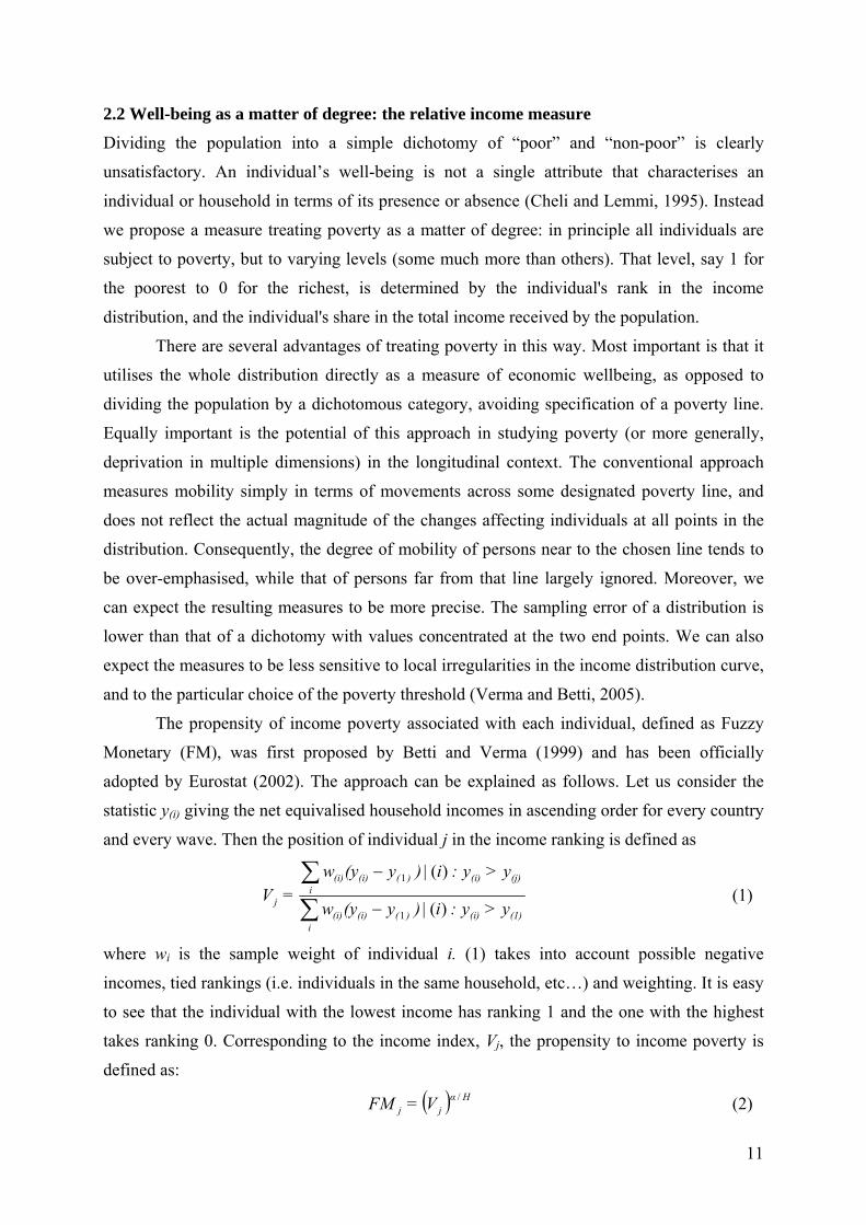
The propensity of income poverty associated with each individual, defined as Fuzzy
Monetary (FM), was first proposed by Betti and Verma (1999) and has been officially
adopted by Eurostat (2002). The approach can be explained as follows. Let us consider the
statistic y(i) giving the net equivalised household incomes in ascending order for every country
and every wave. Then the position of individual j in the income ranking is defined as
(1)(i))(i
(i)(i)
(j)(i))(i
(i)(i)
j y>y:i|)y(yw
y>y:i|)y(yw=V
)(
)(
1
1
−
−
∑∑
(1)
where wi is the sample weight of individual i. (1) takes into account possible negative
incomes, tied rankings (i.e. individuals in the same household, etc…) and weighting. It is easy
to see that the individual with the lowest income has ranking 1 and the one with the highest
takes ranking 0. Corresponding to the income index, Vj, the propensity to income poverty is
defined as:
( ) Hαjj V=FM / (2)
12
where H is the Head Count Ratio for a particular country and a particular wave. The
parameter α is in our case determined such that for the European population as a whole, the
mean of the index FMj is equal to the proportion poor (HCR) according to the conventional
approach. In (2) α is divided by H, since we have empirically found that this form of the
equation results in very stable values of α for different domains despite differences in their
head count ratios (Verma and Betti, 2002).
2.3 A multi-dimensional and comparative perspective: the deprivation index measure
The relative income measure given by (2) overcomes one of the major drawbacks of poverty
status as a measure of well-being, i.e. its simplistic categorisation of population into poor and
non-poor dichotomy. However relative income considers deprivation only in its monetary
dimension, disregarding other non-monetary aspects. This calls for a measure which considers
deprivation in its multiple dimensions (Kolm 1977, Atkinson and Bourguignon 1982, Tsui
1985, Maasoumi 1986, Sen 1999). Certainly, in our application of consequences of marital
disruption, we expect that individuals’ experience of well-being goes beyond a simple drop of
equivalent income: some can experience a dramatic rise in monthly expenses (for example for
paying alimonies) with a substantial change of life-styles. Moreover, a marital disruption is
likely to change, sometimes dramatically, the housing situation of the individuals involved.
Just as in the FM approach described above, we define here the concept of multiple
deprivation as a matter of degree. The state of deprivation is thus seen in the form of ‘fuzzy
sets’ to which all members of the population belong, but to varying degrees. The issue of how
to best summarize items reflecting different dimensions of well-being into a unique index has
been debated (Atkinson et al., 2002; Duclos, Sahn and Younger, 2001; and especially
Atkinson, 2003). A number of authors have evoked the concepts of fuzzy sets in the analysis
of poverty and living conditions (e.g. Chiappero Martinetti 1994; Vero and Werquin 1997).
The present contribution represents a continuation and further development of the work of
Cerioli and Zani (1990), Cheli and Lemmi (1995), Cheli (1995), and Betti and Verma (1999,
2004). In doing so we select a list of items indicating non-monetary deprivation in the
households (see the appendix). These items often take the form of simple ‘yes/no’
dichotomies (such as the presence or absence of enforced lack of certain goods or facilities),
some other items may involve more than two ordered categories, reflecting different degrees
of deprivation. These items are grouped into five different dimensions of deprivation whose
identification is discussed in section 2.4.
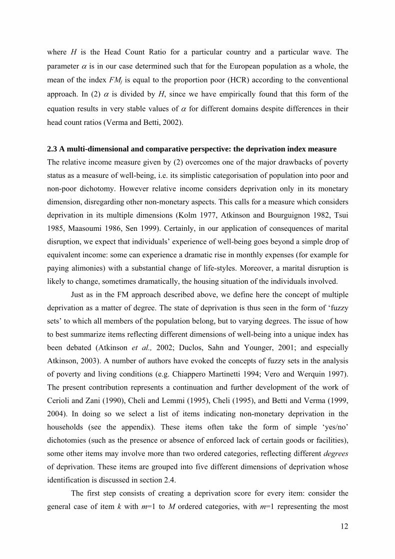
The first step consists of creating a deprivation score for every item: consider the
general case of item k with m=1 to M ordered categories, with m=1 representing the most
13
deprived and m=M the least deprived situation. Let mjk be the category to which individual j
belongs with respect to item k. Cerioli and Zani (1990) assuming that the rank of the
categories represents an equally-spaced metric variable, propose the deprivation score:
1−−
MmM
=d jkjk , Mm jk ≤≤1 (3a)
Cheli and Lemmi (1995) improves on this approach by replacing the simple ranking of the
categories with their distribution function F(.) in the population:
1)(1)(1
FmF
=d jkjk −
− (3b)
Note that the above two formulations for djk are identical in by far the most common case –
that of a dichotomous indicator (M=2), giving a dichotomous m.f. djk= 1 (deprived) or djk= 0
(non-deprived). Thus we choose to use the simpler formulation (3a).
The second step involves determining weights to be assigned to each item of the
deprivation index. This is a crucial part of deprivation index construction and has caused
some debate in the literature. An early attempt to specify an appropriate weighting system was
due to Ram (1982), using principal component analysis, which was also adopted by
Maasoumi and Nickelsburg (1988). Among others, Nolan and Whelan (1996) adopted factor
analysis for evaluating a weighting system, while Cerioli and Zani (1990) and Cheli and
Lemmi (1995) adopted a weighting system based on the diffusion of the individual item (see
also Lemmi and Betti (forthcoming) for further details).
The weighting procedure we propose here is a variant of the procedure developed by
Betti and Verma (1999) and incorporates crucial dimensions of how the items are distributed
in the population. Firstly, the weight is determined by the variable's power to differentiate
among individuals in the population, that is, by its dispersion. This amounts to letting the
weight depend on the coefficient of variation of deprivation score djk , which we define as akw .
In practice this means that items that affect only small proportions of the population are
considered more critical, and therefore given a larger weight. Secondly, in order to avoid
redundancy, it is necessary to limit the influence of those characteristics that are highly
correlated with the others included in the analysis. Even for the overall index, it is reasonable
to consider this correlation separately within each of the dimensions of deprivation identified,
i.e., the weight of variable k in deprivation dimension δ is taken as the inverse of an average
measure of its correlation with all the variables in that dimension. There are many examples
where items within a dimension can be correlated. One is the two items relating to possession
14
of a television and a video recorder. It is unlikely that a household will possess a video
recorder unless they possess a television set as well, thus inducing a positive correlation.
Similarly, different items describing the conditions of the dwelling may also be correlated.
For instance, a dwelling plagued by rot in window frames or floors is also more likely to
report to have damp walls, floors and foundations (see Appendix for a detailed description of
the items). However, a household reporting both items should not be counted as being twice
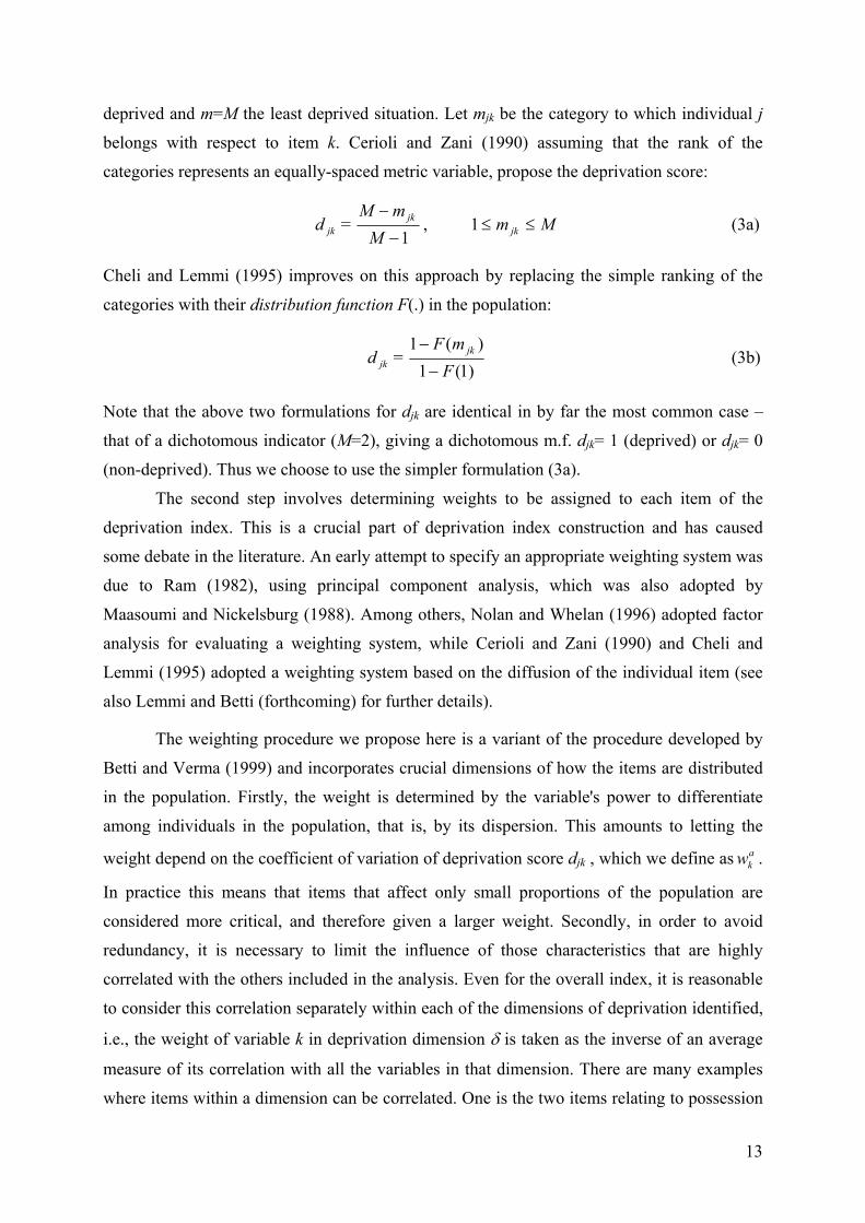
worse off than a household reporting none of these items. Formally the weight can be
expressed as:
⎟⎟⎟⎟
⎠
⎞
⎜⎜⎜⎜
⎝
⎛
≥⋅⎟⎟⎟⎟
⎠
⎞
⎜⎜⎜⎜
⎝
⎛
∝
∑∑K
=k'Hk'k,k'k,
K
=k'Hk'k,k'k,
bkρρ|ρρ<ρ|ρ+
w
11
1
1
1 (4)
where ),( jk'jkk'k, ddcorr=ρ is the correlation between the two deprivation scores. In the first
term in the right side of (3), the sum is taken over all indicators whose correlation with the
variable k is less than a certain value ρh (determined, for instance, by dividing the ordered set
of correlation values at the point of the largest gap.). Thus the results are not affected by
arbitrary inclusion or exclusion of items highly correlated with other items in the set. The
final weight is then given as: ∝kw akw x b
kw (see Betti and Verma (2002) for further details).
With these weights, a deprivation score is determined for the overall situation covering all the
indicators:
( )∑
∑ −
kk
kjkk
j w
dw=S
1 (5)
Note that (5) defines a 'positive' score indicating lack of deprivation.
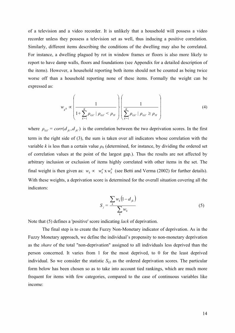
The final step is to create the Fuzzy Non-Monetary indicator of deprivation. As in the
Fuzzy Monetary approach, we define the individual’s propensity to non-monetary deprivation
as the share of the total "non-deprivation" assigned to all individuals less deprived than the
person concerned. It varies from 1 for the most deprived, to 0 for the least deprived
individual. So we consider the statistic S(j) as the ordered deprivation scores. The particular
form below has been chosen so as to take into account tied rankings, which are much more
frequent for items with few categories, compared to the case of continuous variables like
income:
15
(1)(i)i
(i)(i)
(j)(i)i
(i)(i)
j S>S:i|Sw
S>S:i|Sw=FS
)(
)(
∑∑
. (6)
It should be taken in mind that w(i) in the (6) is different from wk in the (5), being the first the
individual sampling weight and second the weight of item k as defined earlier.
2.4 Dimensions of non-monetary deprivation
Supplementing the overall deprivation measure introduced above, it is useful to
identify the underlying dimensions and to group the indicators accordingly. Taking into
account the manner in which different indicators cluster together adds to the richness of the
analysis; ignoring such dimensionality can in fact result in misleading conclusions. Thus we
want to analyse not only the overall deprivation index as defined in (6) but also the
deprivation indices for each dimension of well-being. Approaches of this kind applied to
poverty analysis of European countries are becoming more common. By applying a factor
analysis based on 24 variables in the ECHP, also the Eurostat (2002) Report identifies five
groups, for which it constructs deprivation indices. In a similar approach Aassve et al. (2005)
consider the impact of childbearing events on a similar set of deprivation indices.
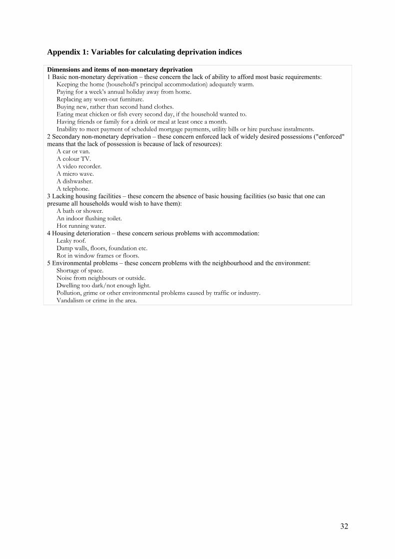
Here we identify five dimensions of deprivation, all of which derived from factor
analysis (see Whelan et al. 2001 for details). We define, for each dimension δ: 1,…, Δ and for
each individual j, the deprivation score Sj,δ as in (5) but only considering the items belonging
to dimension δ. The individual’s propensity to deprivation FSj,δ is defined as in (6) taking the
ordered values S(j),δ . This means that the average value of the overall deprivation index is
allowed to vary from one dimension to another, reflecting the relative prevalence of each.
The dimensions are as follows: (1) basic non-monetary deprivation; (2) secondary non-
monetary deprivation; (3) lack of housing facilities; (4) housing deterioration; and (5)
environmental problems. The list of items used to construct the deprivation indices for each of
these dimensions are reported in the appendix.
3. Data and estimation strategy
3.1 Data and definition of marital breakdown

16
The European Community Household Panel (ECHP) is a set of comparable large-scale
longitudinal studies implemented by the European Union. The first wave of the ECHP was
collected in 1994 for the original countries in the survey: Germany, Denmark, the
Netherlands, Belgium, Luxembourg, France, the UK, Ireland, Italy, Greece, Spain and
Portugal. Three countries were late joiners to the project: Austria joined in 1995, Finland in
1996 and Sweden in 1997. All countries except Luxembourg, Sweden and Germany are
included in the analysis; Luxembourg is omitted because of an extremely small sample,
Sweden because the data do not form a panel, Germany is dropped because the information
necessary to construct the deprivation indices is not available for this country. Eight waves of
the ECHP were collected in total, the last collected in 2001. We aggregate data according the
welfare regime clusters defined by Esping-Andersen (1990, 1999) and Trifiletti (1999); the
clusters are as follows: Liberal countries (United Kingdom and Ireland), Social Democratic
countries (Finland and Denmark), Conservative countries (Belgium, Netherlands, France, and
Austria), and Mediterranean countries (Italy, Spain, Portugal, and Greece).
The event of interest is marital dissolution that is defined by separation or a divorce,
and in the ECHP the variable is based on self reported marital status, and household
composition. A marital split materialises in most cases as a separation between partners,
followed by a formal divorce. Laws and regulations on separation and divorce vary across
European countries. One important implication of this is that the duration between separation
and divorce will differ, which in turn implies that the well-being for individuals currently
separated may be different from the well-being of those defined as divorced. Since in most
cases a separation is associated with a significant financial shock, it is likely that separated
individuals, especially women, have a high likelihood of experiencing deterioration in their
financial well-being. The financial strain associated with a divorce (as opposed to a
separation) is likely to be less severe for divorced individuals, since this will normally take
place some time after the physical separation. As such, we would expect poverty and
deprivation to be lower than for those registered as divorced. Of importance in this analysis is
to measure the event in which a couple physically ceased to live in the same household. Thus,
a couple, in our analysis, is not formally recorded as separated unless they also reported to
live in separate households. We make this distinction since they in this situation cannot
benefit from economies of scale of the household, nor can they share the burdens of rearing
children.

17
3.2 Propensity score matching
In estimating the effect of marital disruption on economic wellbeing we face the
potential problem of selection bias. That is, couples experiencing a marital separation may be
qualitatively different from couples not separating. For example, women who are strongly
dependent on partner’s income are probably less likely to separate from them as they are
aware of the strong economic distress they would experience in the case they split from their
partner (Becker, 1991). Here we tackle this issue by implementing a propensity score
matching technique. Applications of this kind are growing in literature (see among others
Blundell et al. 2005; Lechner, 2002; Dehejia and Wahba, 1998) beyond the evaluation of
social programmes. In our setting we assume that each individual i has two potential
outcomes, Y1i in the case he/she experiences a marital split (the treatment) and Y0i in the case
he/she does not (the controls). The causal impact is given by the comparison between Y1i and
Y0i. Obviously, only one of these two outcomes is observable for every individual making
such a comparison impossible, a problem often referred to as the “fundamental problem of
causal inference” (Holland, 1986).
Let Di be the treatment variable taking the value 1 if individual i receives the treatment
(marital split) and 0 otherwise. One parameter of interests is commonly referred to as average
treatment effect on treated (ATET) that is:
ATET ≡ E(Y1i|Di = 1) - E(Y0i|Di = 1) (7)
In (7) we have to identify of E(Y0i|Di = 1). This needs further assumption on the
selection process. The easiest solution is using a naïve estimator of ATET consisting of
observed difference between treated and control groups:
ATET = E(Y1i|Di = 1) - E(Y0i|Di = 0) (8)
(8) assumes that there is no selection bias, i.e. treated group is randomly selected from the
total population. It is well known that in observational studies this assumption is overly strong
and treated and control groups are systematically different, so that (8) is a biased estimate of
ATET. Lalonde (1986) use B = E(Y1i|Di = 1) - E(Y0i|Di = 0) as a measure of the bias term
while Heckman et al. (1998) propose to write B as a function of a set of observed variables X:
18
∫∫ −0X
0
1X
0 0011SS
)=D|)dF(X=DX,|E(Y)=D|)dF(X=DX,|E(Y=B (9)
where )=DX,|E(Y)=DX,|E(Y=B(X) 01 00 − is the pointwise selection bias in X. Based on
(9) Heckman et al. (1998) derive a decomposition of B into three terms B1, B2, and B3.
Term B1 arises when the supports of the observable X for the treated and the control group S1X
and S0X are not overlapping, i.e. among the treated group we observe value of X that are not
observed in the control group or vice versa. Term B2 depends on misweighting within the
common support, since the distribution of X may change when we restrict to common support.
Finally, term B3 is the true “selection” bias term arising from a different distribution of
unobserved variables between treated and untreated.
The removal of the bias terms from the (9) is then the crucial part of the estimation
strategy. Here we use a matching method, based on the critical assumption called conditional
independence assumption (CIA) stating that treatment status is random conditional on some
set of X, in notation
X|DY ⊥0 (10)
If CIA holds the bias in (9) only depends from observed variables X and B3 is zero. Under this
assumption, EX (Y0i| Xi, Di=0) = EX (Y0i| Xi, Di=1), thus the ATET can be unbiasedly estimated
by
ATET= EX (Y1i - Y0i| Xi, Di=1) = EX (Y1i| Xi, Di=1) -EX (Y0i| Xi, Di=0). (11)
Though theoretically appealing, the matching approach is in practice difficult to apply when
the dimension of X is high because of the difficulties in calculating the conditional
expectations in the (11). Instead of matching on the base of X one can equivalently match
treated and comparison units on the base of any balancing score, and in particular on the base
of the “propensity score” (Rosenbaum and Rubin 1983) that is the conditional probability of
receiving the treatment given the values of X, formally:
p(Xi) = Pr(Di = 1|Xi) (12)
This result reduces the dimensionality problem in computing the conditional
expectation and an unbiased estimate of ATET can be found from:
[ ]{ }10,1,ATET 01 =D|p(X))=D|E(Yp(X))=D|E(YE= p(X) − (13)
There are many matching estimators (see, for example Becker and Ichino, 2002; and Smith
and Todd, 2005), all of them can be seen as generated by the following formula
{ }{ }∑ ∑
∈ ∈ ⎥⎥
⎦
⎤
⎢⎢
⎣
⎡⋅−
1 0
10j1i
1 = =YwY
n=ATET
iDi JDjij (14)
19
where the weight wij is defined according the matching method is used. In this work we
implement a nearest neighbour matching consisting of pairing every treated unit with the
closest control unit, i.e. weight is defined as
|])P(X)P(X| ij − (15)
Sometimes it may happen that more than k>1 controls satisfy the (15). In this case we
use all these k controls with weight 1/k. Thus two out of three components sources of bias in
(9) are eliminated. B1 is eliminated by allowing matches only in the common support region,
and B2 is eliminated because the control units are re-weighted according the value of p(X). B3
is the only component of (9) that is not eliminated by matching and it is assumed to be zero by
CIA. Also CIA, albeit less strong than the assumption underlying the naïve estimator, has
proved to be unlikely to hold. Based on this Heckman et al. (1998) propose to combine a
Difference-in-Differences (DD) estimator to the matching procedure. In essence this implies
comparing the mean change of well-being from one time period t to another, t+1, of
participants, with the mean change of well-being for the same time period for non-participant.
)()()()( 0101
011
1 ΔEΔE=YYEYYE=DD t+tt+t −−−− (16)
An important advantage of the DD estimator is that it allows us to control for selection
into the treatment group caused by unobserved variables. That is, provided unobserved
heterogeneity is time-fixed, its effect will be netted out by taking first difference. In this way
the CIA is relaxed and the critical identifying assumption is now (Heckman et al., 1998)
Bt+1(X)-Bt(X) = 0. (17)
As a result it has been argued that the DD-PSM estimator is more robust since it
eliminates temporarily-invariant sources of bias (e.g. Dehejia and Wahba, 1998, 1999 and
Smith and Todd, 2005). The final estimator of the impact of marital split on well-being is
given by:
[ ]{ }10,1, 01 =D|p(X))=D|E(Δp(X))=D|E(ΔE=PSMDD p(X) −− (18)
DID estimator is implemented in all the estimates. However when we estimate the
effect of separation on poverty status, DID and cross-sectional estimators are equivalent given
that all those who are poor before the marital split are ruled out from analysis. This means that
Yt=0 for all individuals.
The estimation of standard errors of ATET is not a trivial exercise; the main problem
is that the estimated variance of ATET should also include the variance due to estimation of
the propensity score. The common solution to this problem is bootstrapping (see for example,
Lechner, 2002 and Blundell et al., 2005). This is the solution we adopt, using the module
developed by Leuven and Sianesi (2003) for STATA.

20
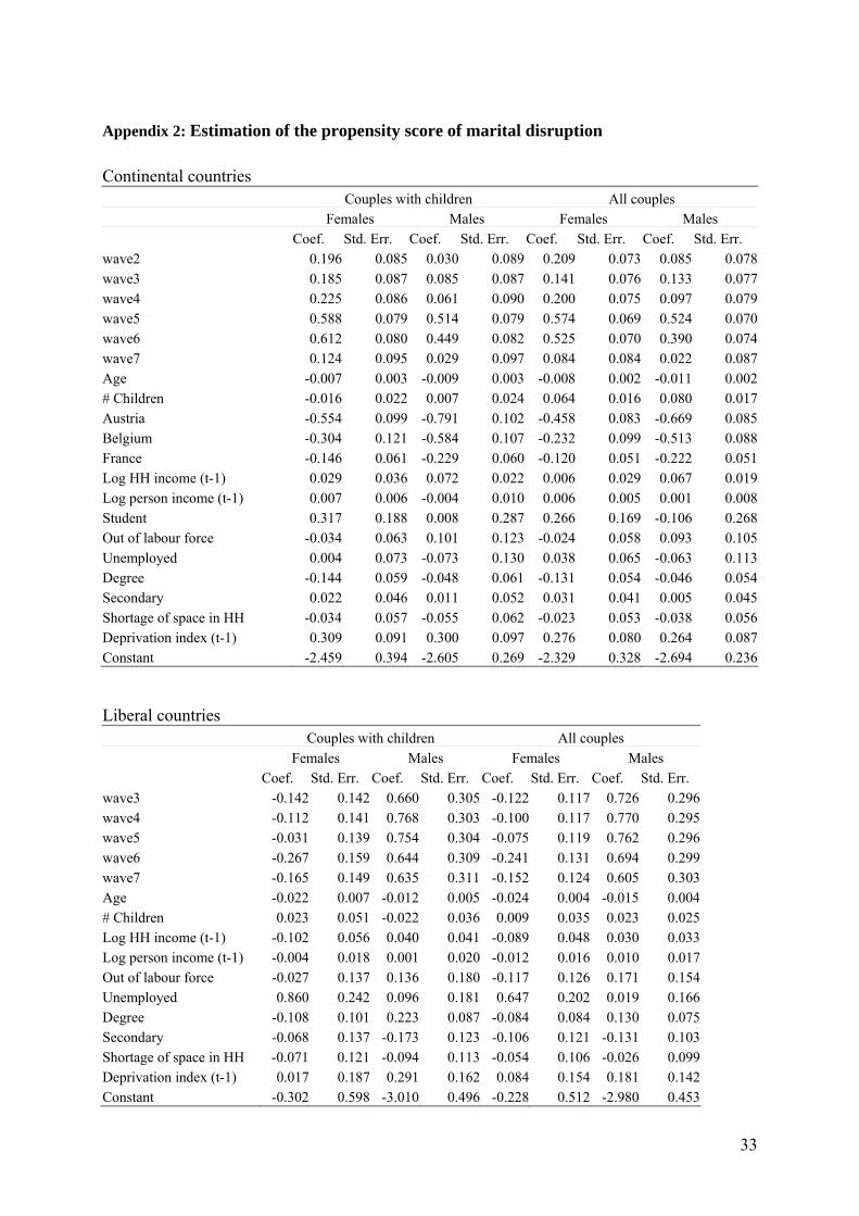
The matching procedure based on the PSM implies that all variables have to be
balanced between treated and control units. In order to satisfy the balancing property, the
propensity score specification changes with the country specific samples (see estimates in
appendix). In all samples the variables which are suspected to confound the effect of marital
split on poverty are included in the estimation of the propensity score: wave, age, number of
children, well-being level prior the event (measured both in terms of income and in terms of
deprivation), education and employment status. It has to be kept in mind that the main
purpose of propensity score estimation is not to predict participation to treatment but to
balance all covariates in the matching procedure (Augurzky and Schmidt, 2000). Therefore
we are not interested in goodness of fit of model specification but in balancing all observed
variables. Moreover “perfect” prediction should be avoided since if P(X)=0 or P(X)=1 for
some value of X we cannot match on these values of X as they are out of the common support.
Heckman et al. (1998) argue that some randomness is needed in order to guarantee to observe
individuals with identical values of X both in the treatment and the control groups. Then after
having chosen the appropriate variables to include in the propensity score estimate we test
whether the balancing property is satisfied for each model specification we used. The null
hypothesis (i.e. covariates are balanced between treated and untreated) is rejected in non of
the cases.
4. Results
4.1 Entering Poverty
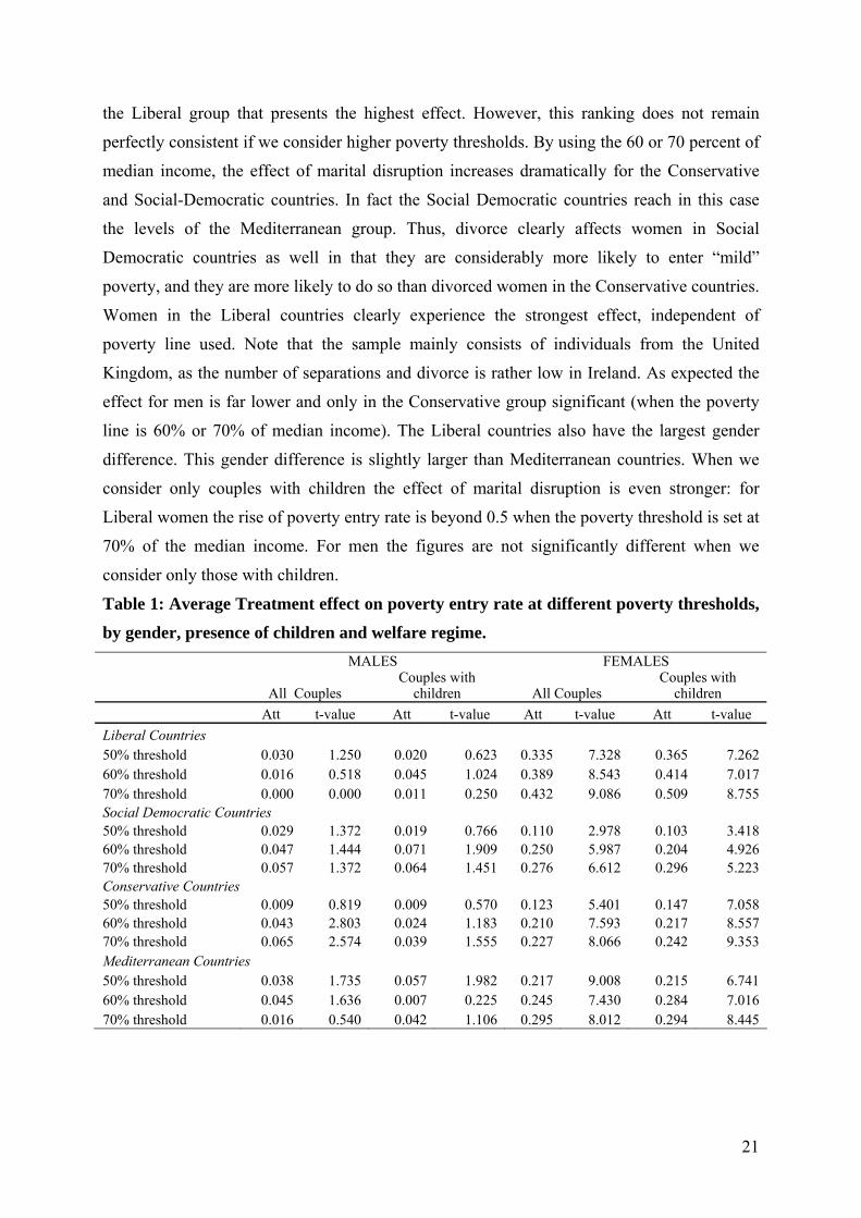
Table 1 presents the effects of experiencing a divorce/separation event on entering
poverty using different poverty thresholds. Note that the estimate refers to what is called the
average treatment effect on the treated, and reflects therefore the difference between the rate
of entering poverty for married couples and individuals experiencing a marital break-up.
The results confirm that women are considerably more likely to enter poverty as a
result of divorce compared to men. This is the case independent of countries and poverty
threshold used. Moreover, the effects are largely consistent with welfare regime theory.
Especially with the 50 percent threshold, the ranking of country groups is perfectly in line
with the Welfare Regime theory, having the Social-Democratic group the smallest effect
followed in ascending order by the Conservative countries, the Mediterranean, and, finally,
21
the Liberal group that presents the highest effect. However, this ranking does not remain
perfectly consistent if we consider higher poverty thresholds. By using the 60 or 70 percent of
median income, the effect of marital disruption increases dramatically for the Conservative
and Social-Democratic countries. In fact the Social Democratic countries reach in this case
the levels of the Mediterranean group. Thus, divorce clearly affects women in Social
Democratic countries as well in that they are considerably more likely to enter “mild”
poverty, and they are more likely to do so than divorced women in the Conservative countries.
Women in the Liberal countries clearly experience the strongest effect, independent of
poverty line used. Note that the sample mainly consists of individuals from the United
Kingdom, as the number of separations and divorce is rather low in Ireland. As expected the
effect for men is far lower and only in the Conservative group significant (when the poverty
line is 60% or 70% of median income). The Liberal countries also have the largest gender
difference. This gender difference is slightly larger than Mediterranean countries. When we
consider only couples with children the effect of marital disruption is even stronger: for
Liberal women the rise of poverty entry rate is beyond 0.5 when the poverty threshold is set at
70% of the median income. For men the figures are not significantly different when we
consider only those with children.
Table 1: Average Treatment effect on poverty entry rate at different poverty thresholds,
by gender, presence of children and welfare regime. MALES FEMALES
All Couples Couples with
children All Couples Couples with
children Att t-value Att t-value Att t-value Att t-value Liberal Countries 50% threshold 0.030 1.250 0.020 0.623 0.335 7.328 0.365 7.262 60% threshold 0.016 0.518 0.045 1.024 0.389 8.543 0.414 7.017 70% threshold 0.000 0.000 0.011 0.250 0.432 9.086 0.509 8.755 Social Democratic Countries 50% threshold 0.029 1.372 0.019 0.766 0.110 2.978 0.103 3.418 60% threshold 0.047 1.444 0.071 1.909 0.250 5.987 0.204 4.926 70% threshold 0.057 1.372 0.064 1.451 0.276 6.612 0.296 5.223 Conservative Countries 50% threshold 0.009 0.819 0.009 0.570 0.123 5.401 0.147 7.058 60% threshold 0.043 2.803 0.024 1.183 0.210 7.593 0.217 8.557 70% threshold 0.065 2.574 0.039 1.555 0.227 8.066 0.242 9.353 Mediterranean Countries 50% threshold 0.038 1.735 0.057 1.982 0.217 9.008 0.215 6.741 60% threshold 0.045 1.636 0.007 0.225 0.245 7.430 0.284 7.016 70% threshold 0.016 0.540 0.042 1.106 0.295 8.012 0.294 8.445
22
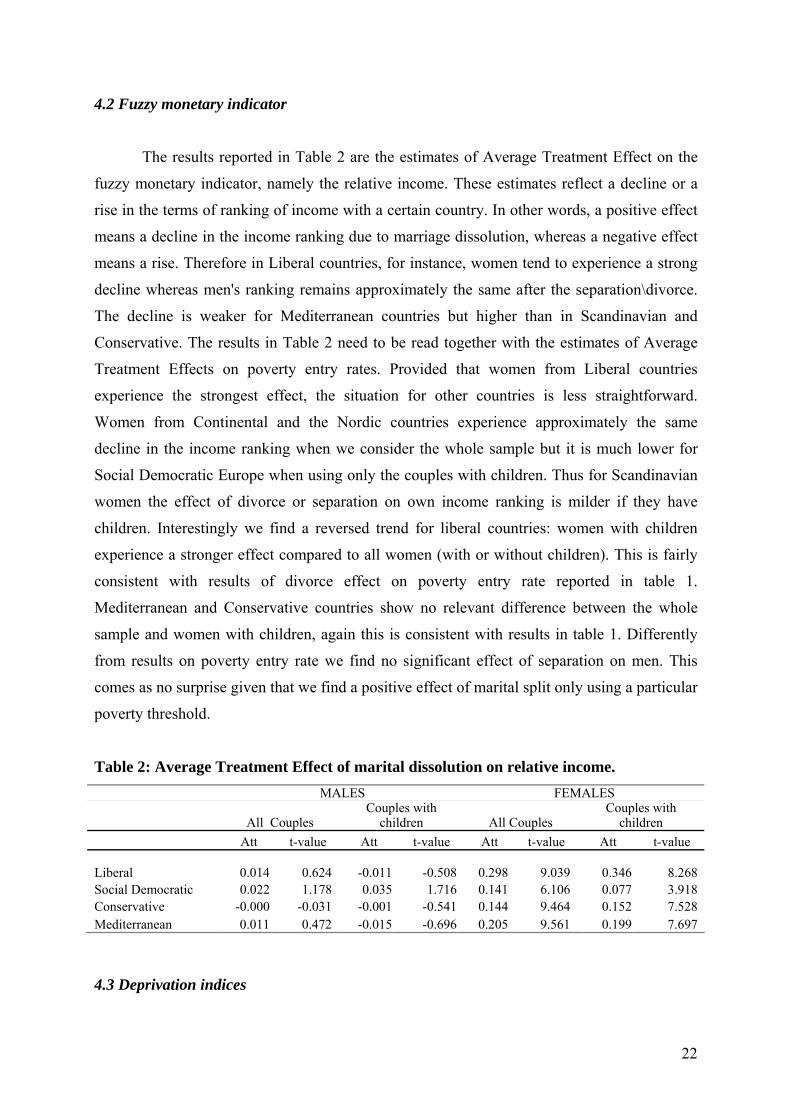
4.2 Fuzzy monetary indicator
The results reported in Table 2 are the estimates of Average Treatment Effect on the
fuzzy monetary indicator, namely the relative income. These estimates reflect a decline or a
rise in the terms of ranking of income with a certain country. In other words, a positive effect
means a decline in the income ranking due to marriage dissolution, whereas a negative effect
means a rise. Therefore in Liberal countries, for instance, women tend to experience a strong
decline whereas men's ranking remains approximately the same after the separation\divorce.
The decline is weaker for Mediterranean countries but higher than in Scandinavian and
Conservative. The results in Table 2 need to be read together with the estimates of Average
Treatment Effects on poverty entry rates. Provided that women from Liberal countries
experience the strongest effect, the situation for other countries is less straightforward.
Women from Continental and the Nordic countries experience approximately the same
decline in the income ranking when we consider the whole sample but it is much lower for
Social Democratic Europe when using only the couples with children. Thus for Scandinavian
women the effect of divorce or separation on own income ranking is milder if they have
children. Interestingly we find a reversed trend for liberal countries: women with children
experience a stronger effect compared to all women (with or without children). This is fairly
consistent with results of divorce effect on poverty entry rate reported in table 1.
Mediterranean and Conservative countries show no relevant difference between the whole
sample and women with children, again this is consistent with results in table 1. Differently
from results on poverty entry rate we find no significant effect of separation on men. This
comes as no surprise given that we find a positive effect of marital split only using a particular
poverty threshold.
Table 2: Average Treatment Effect of marital dissolution on relative income. MALES FEMALES
All Couples Couples with
children All Couples Couples with
children Att t-value Att t-value Att t-value Att t-value Liberal 0.014 0.624 -0.011 -0.508 0.298 9.039 0.346 8.268 Social Democratic 0.022 1.178 0.035 1.716 0.141 6.106 0.077 3.918 Conservative -0.000 -0.031 -0.001 -0.541 0.144 9.464 0.152 7.528 Mediterranean 0.011 0.472 -0.015 -0.696 0.205 9.561 0.199 7.697
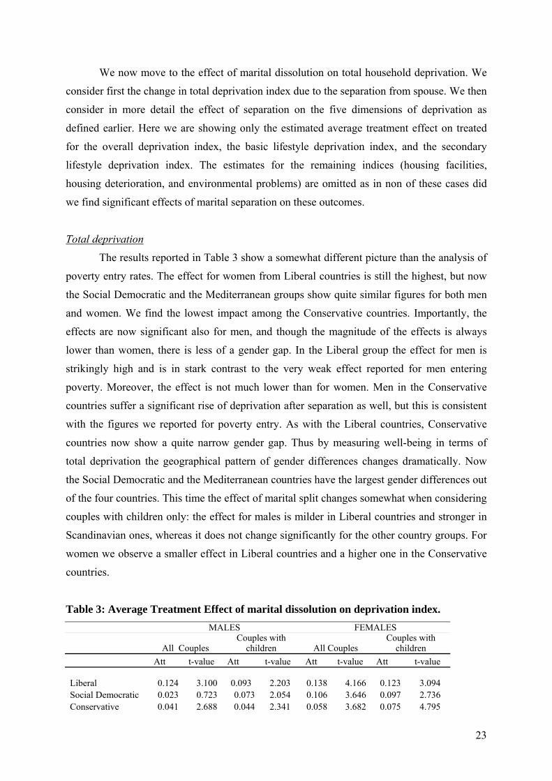
4.3 Deprivation indices
23
We now move to the effect of marital dissolution on total household deprivation. We
consider first the change in total deprivation index due to the separation from spouse. We then
consider in more detail the effect of separation on the five dimensions of deprivation as
defined earlier. Here we are showing only the estimated average treatment effect on treated
for the overall deprivation index, the basic lifestyle deprivation index, and the secondary
lifestyle deprivation index. The estimates for the remaining indices (housing facilities,
housing deterioration, and environmental problems) are omitted as in non of these cases did
we find significant effects of marital separation on these outcomes.
Total deprivation
The results reported in Table 3 show a somewhat different picture than the analysis of
poverty entry rates. The effect for women from Liberal countries is still the highest, but now
the Social Democratic and the Mediterranean groups show quite similar figures for both men
and women. We find the lowest impact among the Conservative countries. Importantly, the
effects are now significant also for men, and though the magnitude of the effects is always
lower than women, there is less of a gender gap. In the Liberal group the effect for men is
strikingly high and is in stark contrast to the very weak effect reported for men entering
poverty. Moreover, the effect is not much lower than for women. Men in the Conservative
countries suffer a significant rise of deprivation after separation as well, but this is consistent
with the figures we reported for poverty entry. As with the Liberal countries, Conservative
countries now show a quite narrow gender gap. Thus by measuring well-being in terms of
total deprivation the geographical pattern of gender differences changes dramatically. Now
the Social Democratic and the Mediterranean countries have the largest gender differences out
of the four countries. This time the effect of marital split changes somewhat when considering
couples with children only: the effect for males is milder in Liberal countries and stronger in
Scandinavian ones, whereas it does not change significantly for the other country groups. For
women we observe a smaller effect in Liberal countries and a higher one in the Conservative
countries.
Table 3: Average Treatment Effect of marital dissolution on deprivation index. MALES FEMALES
All Couples Couples with
children All Couples Couples with
children Att t-value Att t-value Att t-value Att t-value Liberal 0.124 3.100 0.093 2.203 0.138 4.166 0.123 3.094 Social Democratic 0.023 0.723 0.073 2.054 0.106 3.646 0.097 2.736 Conservative 0.041 2.688 0.044 2.341 0.058 3.682 0.075 4.795

24
Mediterranean 0.034 1.137 0.036 1.112 0.115 4.860 0.105 3.831
Basic Lifestyle deprivation
If we focus on the first dimension of deprivation, i.e. deprivation on basic lifestyle, we
find results relatively consistent with results for total deprivation index. Again the liberal
group shows the strongest effect both for men and women, but this time the effect for women
is about twice as high. The weakest effect is found in Mediterranean countries even though
the effect for the Conservative group is almost equal. Again for the Scandinavian countries we
notice a relatively high effect for women and a significant gender gap. Finally, we register as
before a significant effect for men also in the Conservative group.
The presence of children seems to negatively influence the effect for males: apart from
Mediterranean countries, almost everywhere the effect of marital split is stronger when we
only consider couples with children. Conversely, the effect for women is almost everywhere
weaker, with the exception of Conservative countries.
Table 4: Average Treatment Effect of marital dissolution on basic lifestyle deprivation
index. MALES FEMALES
All Couples Couples with
children All Couples Couples with
children Att t-value Att t-value Att t-value Att t-value Liberal 0.114 2.785 0.136 2.178 0.224 4.541 0.194 3.303 Social Democratic 0.033 0.850 0.100 2.251 0.166 3.646 0.104 2.173 Conservative 0.086 4.840 0.089 3.904 0.127 6.010 0.145 5.881 Mediterranean 0.025 0.809 0.024 0.613 0.126 4.374 0.118 3.988
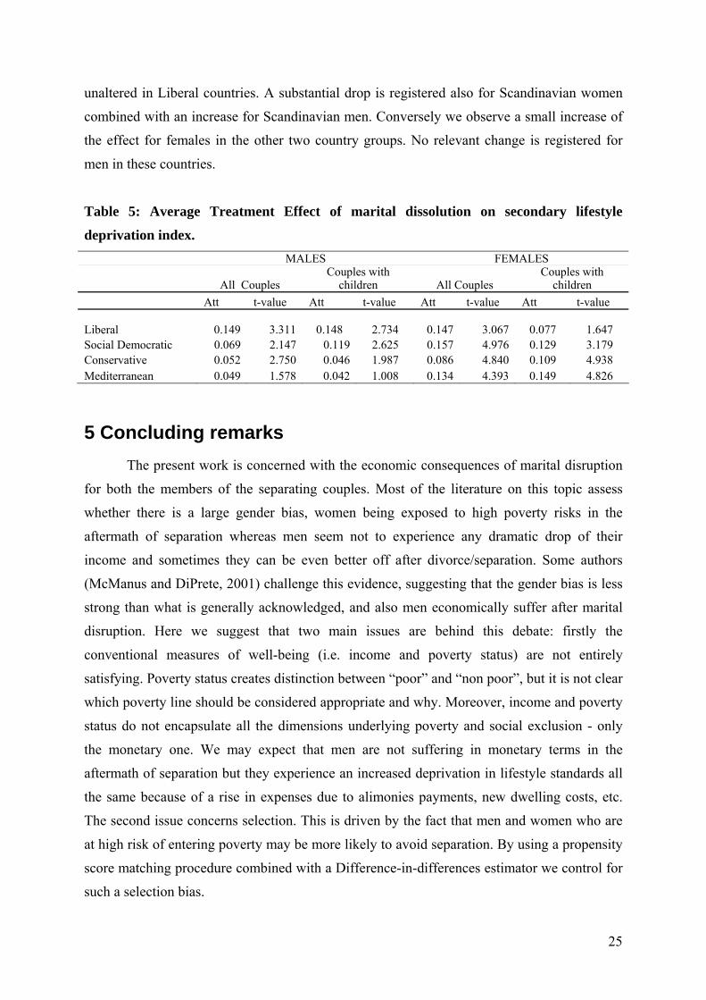
Secondary lifestyle deprivation
Finally, we look at the effects of marital disruption on the deprivation level concerning
the secondary lifestyle deprivation. Surprisingly we find the strongest effect for women in the
Scandinavian countries and not in Liberal ones (whose estimate however is, together with
Mediterranean countries, quite close to the Scandinavian group). The effect in the Continental
countries is much lower. Another interesting feature of these results is the effect of separation
for men, which is now quite close to deprivation for women, i.e. the gender gap is reduced
when considering secondary lifestyle deprivation.
Again, if we consider couples with children only, the results change somewhat.
Surprisingly the effect for women is no longer significant whereas for men it remains
25
unaltered in Liberal countries. A substantial drop is registered also for Scandinavian women
combined with an increase for Scandinavian men. Conversely we observe a small increase of
the effect for females in the other two country groups. No relevant change is registered for
men in these countries.
Table 5: Average Treatment Effect of marital dissolution on secondary lifestyle
deprivation index. MALES FEMALES
All Couples Couples with
children All Couples Couples with
children Att t-value Att t-value Att t-value Att t-value Liberal 0.149 3.311 0.148 2.734 0.147 3.067 0.077 1.647 Social Democratic 0.069 2.147 0.119 2.625 0.157 4.976 0.129 3.179 Conservative 0.052 2.750 0.046 1.987 0.086 4.840 0.109 4.938 Mediterranean 0.049 1.578 0.042 1.008 0.134 4.393 0.149 4.826
5 Concluding remarks The present work is concerned with the economic consequences of marital disruption
for both the members of the separating couples. Most of the literature on this topic assess
whether there is a large gender bias, women being exposed to high poverty risks in the
aftermath of separation whereas men seem not to experience any dramatic drop of their
income and sometimes they can be even better off after divorce/separation. Some authors
(McManus and DiPrete, 2001) challenge this evidence, suggesting that the gender bias is less
strong than what is generally acknowledged, and also men economically suffer after marital
disruption. Here we suggest that two main issues are behind this debate: firstly the
conventional measures of well-being (i.e. income and poverty status) are not entirely
satisfying. Poverty status creates distinction between “poor” and “non poor”, but it is not clear
which poverty line should be considered appropriate and why. Moreover, income and poverty
status do not encapsulate all the dimensions underlying poverty and social exclusion - only
the monetary one. We may expect that men are not suffering in monetary terms in the
aftermath of separation but they experience an increased deprivation in lifestyle standards all
the same because of a rise in expenses due to alimonies payments, new dwelling costs, etc.
The second issue concerns selection. This is driven by the fact that men and women who are
at high risk of entering poverty may be more likely to avoid separation. By using a propensity
score matching procedure combined with a Difference-in-differences estimator we control for
such a selection bias.
26
We expect that by using different measures of well-being we are able to observe that
both men and women experience an economic deprivation after separation being women more
deprived in monetary terms and men in non monetary terms. The results confirm largely to
our expectations: it is confirmed that the definition of poverty threshold is an important issue.
Results differ considerably depending on whether we use a 50%, a 60%, or 70% poverty line.
Moreover when we use monetary measures (i.e. poverty status and relative income) it is
unquestionable that women suffer a disproportionately larger negative effect than men. Also
important is that by using monetary measures, we find that most of the results are consistent
with welfare regime theory. However, the non-monetary measures (i.e. deprivation indices)
provide a different picture. Women are still found to suffer significantly more than men, but it
is also clear that men's level of deprivation also increases, and in some cases there is no
significant difference between the ATT estimated for men and women (this is case in Liberal
countries when using the overall deprivation index and the secondary lifestyle deprivation
index).
Children play an important role in explaining the gender differences. If there are
children in the conjugal dwelling, then mothers are much more likely to be granted custody
following a divorce. Thus the divorce event will for many women imply reduced income
(poorer access to the husband’s income) and a higher relative expenditure. Men are instead
likely to live alone or with parents, and are much less likely to experience poverty and
financial strain. Considering couples with children only in the analysis of entering poverty, we
notice that in Liberal and Mediterranean countries the gender gap is even larger, in
Scandinavian countries is smaller, and in the Conservative countries it remains, more or less
unaltered.
However, in terms of deprivation, men do suffer significantly. Many of the items used
to compute the deprivation index refers to characteristics of the dwelling. If it is the case that
men normally has to leave the dwelling following a divorce, he will in the short run at least,
loose out on many of the goods and services that the household would provide. So though
men are not worse off financially, they are worse off in terms of consumer durables and
certain expenditure goods. It also seems likely that the new dwelling is often of poorer quality
of the original dwelling, which is consistent with our estimates.
The gender difference is clearly smaller when children are not present in the dwelling.
With no children, the effect on lifestyle deprivation among men becomes higher, whereas it is
slightly smaller for women. One important factor here is that it is less clear which of the
spouses that will stay put in the conjugal dwelling if the couple has no children.
27
References Aassve A., Mazzuco S. and Mencarini L. (2005) Childbearing and well-being: a comparative
analysis of European welfare regimes. Journal of European Social Policy, 15, 283
299.
Andreß H.J., Borgloh B., Bröckel M., Giesselmann M., Hummelsheim D. (2004) The
economic consequences of partnership dissolution A comparative analysis of panel
studies from five European countries. Paper presented at the 3rd Conference of the
European Research Network on Divorce, December 2 – 4, 2004 in Cologne/Germany.
Atkinson A.B. (2003) Multidimensional deprivation: contrasting social welfare and counting
approaches. Journal of Economic Inequality, 1, 51 65.
Atkinson A.B. and Bourguignon F. (1982) The comparison of multidimensional distributions
of economic status. Review of Economic Studies, 49, 183 201.
Atkinson A.B., Cantillon B., Marlier E. and Nolan B. (2002) Social Indicators: The EU and
Social Inclusion, Oxford University Press, Oxford.
Augurzky, B. and Schmidt, C. (2001) The Propensity Score: A Means to an End, Institute for
the Study of Labour (IZA) Discussion Paper number 271, March, Bonn.
Becker G. S. (1991) A Treatise on Family Harvard University Press, Cambridge, Mass
Becker S. and Ichino A. (2002) Estimation of average treatment effects based on propensity
scores. The STATA Journal.
Betti G. and Verma V. (1999) Measuring the degree of poverty in a dynamic and comparative
context: a multi-dimensional approach using fuzzy set theory. Proceedings, ICCS-VI,
11, pp. 289 301, Lahore, Pakistan.
Betti, G. and Verma V. (2004) A methodology for the study of multi-dimensional and
longitudinal aspects of poverty and deprivation. Università di Siena, Dipartimento di
Metodi Quantitativi, Working Paper 49.
Blundell, R, Dearden, L. and Sianesi, B. (2005) Evaluating the effect of education on
earnings: Models, methods and results from the National Child Development Survey.
Journal of the Royal Statistical Society, Series A, 168, 3, 473 512.
Bourguignon F. and Chakravarty S.R. (2003) The measurement of multidimensional poverty. Journal of Economic Inequality, 1, 25 49.
Browning, M., Bourguignon, F., Chiappori, P. A. and Lechene, V. (1994) Income and
Outcomes: a Structural Model of Intra-household Allocation. Journal of Political
Economy 102 (6), 1067 1096.
28
Burkhauser, R. V., Duncan, G. J., Hauser, R. and Berntsen, R. 1991 Wife or Frau, women do
worse: a comparison of men and women in the United States and Germany after
marital disruption. Demography, 28, 353 360.
Cerioli A. and Zani S. (1990) A Fuzzy Approach to the Measurement of Poverty, in Dagum
C. and Zenga M. (eds.), Income and Wealth Distribution, Inequality and Poverty,
Studies in Contemporary Economics. Berlin: Springer Verlag, pp. 272-284.
Cheli B. (1995) Totally Fuzzy and Relative Measures in Dynamics Context. Metron, 53, pp.
83-205.
Cheli B. and Lemmi A. (1995) A Totally Fuzzy and Relative Approach to the
Multidimensional Analysis of Poverty. Economic Notes, 24, pp. 115-134.
Chiappero Martinetti E. (1994) A new approach to evaluation of well-being and poverty by
fuzzy set theory. Giornale degli Economisti e Annali di Economia, 53, pp. 367-388.
De Vos, K. and Zaidi, A. M. (1997) Equivalence Scale Sensitivity of Poverty Statistics for the
Member States of the European Community. Review of Income and Wealth 43 (3):
319 333 .
Dehejia R, Wahba, S. (1998) Causal Effects in Nonexperimental Studies: Reevaluating the
Evaluation of Training Programs. Journal of the American Statistical Association, 94
(448): 1053 1062.
Dehejia R, Wahba, S. (1999) Propensity Score Matching Methods for Nonexperimental
Causal Studies, NBER Working Paper No. 6829.
Duclos J.-Y., Sahn, D. and Younger, S. D. (2001) Robust multidimensional poverty
comparisons. Université Laval, Canada.
Duncan, G. J. and Hoffman, S. D. (1985) A reconsideration of the economic consequences of
marital dissolution. Demography 22: 485–497.
Esping-Andersen, G. (1990) The Three Worlds of Welfare Capitalism. Princeton, NJ:
Princeton University Press.
Esping-Andersen, G. (1999) The Social Foundations of Post-industrial Economies. Oxford:
Oxford University Press .
Eurostat (2002) European Social Statistics: Income, Poverty and Social Exclusion: 2nd
Report. Luxembourg: Office for Official Publications of the European Communities.
Finnie, R., 1993. Women, men and the economic consequences of divorce: evidence from
Canadian longitudinal data. Canadian Review of Sociology and Anthropology 30, 205
241.
29
Fritzell, J., 1990. The dynamics of income distribution: economic mobility in Sweden in
comparison with the United States. Social Science Research 19: 17–46.
Heckman J.J., Ichimura H., Smith J., Todd P.E. (1998) Matching as an Econometric
Evaluation Estimator: Evidence from Evaluating a Job Training Programme. Review
of Economic Studies 64, 605 654
Holland P.W. (1986) Statistics and Causal Inference. Journal of the American Statistical
Association 81, 945 970.
Jarvis S. and Jenkins S.P. (1999) Marital splits and income changes: evidence from the British
Household Panel Survey. Population Studies, 53 (2), 237 254.
Kolm S.C. (1977) Multidimensional egalitarism, Quarterly Journal of Economics, 91, pp. 1
13.
LaLonde R. (1986) Evaluating the Econometric Evaluations of Training Programs with
Experimental Data. American Economic Review, 76, 604 620.
Lechner M. (2002) Some practical issues in the evaluation of heterogeneous labour market
programmes by matching methods. Journal of the Royal Statistical Society Series A
165(1) 59 82.
Lemmi A. and Betti G. (forthcoming), Fuzzy set approach to multidimensional poverty
measurement, Springer, New York.
Leuven, E. and Sianesi, B. (2003) PSMATCH2: Stata module to perform full Mahalanobis
and propensity score matching, common support graphing, and covariate imbalance
testing. University of Amsterdam and Institute for Fiscal Studies, London.
Lundberg, S., Pollak, R. and Wales, T. J. (1997) Do Husbands and Wives Pool Their
Resourses? Journal of Human Resources 32 (3), 463 480 .
Maasoumi E. (1986) The measurement and decomposition of multidimensional inequality,
Econometrica, 54, pp. 771 779.
Maasoumi E. and Nickelsburg G. (1988) Multivariate measures of well-being and an analysis
of inequality in the Michigan data. Journal of Business & Economic Statistics, 6, pp.
326 334.
Manting D., Bouman A. M. (2004) Short and long term economic consequences of union
dissolution: The case of the Netherlands. Paper presented at the 3rd European
Conference of the Research Network on divorce (Keulen, December 2004).
30
McElroy, M. B. and Horney, M. J. (1981) Nash-bargaining Decisions: Toward a
Generalization of the Theory of Demand. International Economic Review 22 (2): 333
349.
McManus P.A., DiPrete T.A. (2001) Losers and Winners: The Financial Consequences of
Separation and Divorce for Men. American Sociological Review, 66, 246 268.
Nolan B. and Whelan C.T. (1996) Resources, deprivation and poverty. Oxford, Clarendon
Press.
Poortman A., Kalmijn M. (2002), Women’s labour market position and divorce in the
Netherlands: evaluating economic interpretations of the work effect. European
Journal of Population, 18, 175 202.
Poortman, A., 2000. Sex differences in the economic consequences of separation: a panel
study of the Netherlands. European Sociological Review 16: 367 383.
Ram R. (1982) Composite indices of physical quality of life, basic needs fulfilment and
income: A principal component representation. Journal of Development Economics,
11, pp. 227 248.
Rosenbaum P.T. and Donald B. Rubin (1983) The Central Role of the Propensity Score in
Observational Studies for Causal Effects. Biometrika, 70(1), 41 55.
Sen A.K. (1999) Development as freedom, Oxford University Press, Oxford.
Smith J.A., Todd P. (2005), Does Matching Overcome Lalonde's Critique of Nonexperimental
Estimators? Journal of Econometrics, 125(1-2), 305 353.
Smock P.J, Manning W.D., Gupta S. (1999) The Effect of Marriage and Divorce on Women’s
Economic Well-Being. American Sociological Review, 64, 794 812.
Smock, P. J., (1993) The economic costs of marital disruption for young women over the past
two decades. Demography 30: 353 371.
Smock, P. J., (1994) Gender and the short-run economic consequences of marital disruption.
Social Forces 73, 243 62.
Trifiletti, R., (1999) Southern European Welfare Regimes and the Worsening Position of
Women. Journal of European Social Policy, 9(1), 49 64
Tsui K. (1985) Multidimensional generalisation of the relative and absolute inequality indices:
the Atkinson-Kolm-Sen approach. Journal of Economic Theory, 67, 251 265.
Uunk, W., (2004) The Economic Consequences of Divorce for Women in the European
Union: The Impact of Welfare State Arrangements. European Journal of Population,
20, 251 285.
31
Verma V. and Betti G. (2005) Sampling Errors for Measures of Inequality and Poverty.
Invited paper in Classification and Data Analysis 2005 - Book of Short Papers, pp.
175-179, CLADAG, Parma, 6-8 June 2005.
Verma V., Betti G. (2002) Longitudinal measures of income poverty and life-style
deprivation, Working Paper 50, Dipartimento di Scienze Statistiche, University of
Padua.
Vero J. and Werquin P (1997) Reexamining the Measurement of Poverty: How Do Young
People in the Stage of Being Integrated in the Labour Force Manage (in French),
Economie et Statistique, 8-10, 143 156.
Whelan C.T., Layte R., Maitre B. and Nolan B. (2001) Income, deprivation and economic
strain: an analysis of the European Community Household Panel. European
Sociological Review, 17, 357 372.
32
Appendix 1: Variables for calculating deprivation indices Dimensions and items of non-monetary deprivation 1 Basic non-monetary deprivation – these concern the lack of ability to afford most basic requirements: Keeping the home (household’s principal accommodation) adequately warm. Paying for a week’s annual holiday away from home. Replacing any worn-out furniture. Buying new, rather than second hand clothes. Eating meat chicken or fish every second day, if the household wanted to. Having friends or family for a drink or meal at least once a month. Inability to meet payment of scheduled mortgage payments, utility bills or hire purchase instalments. 2 Secondary non-monetary deprivation – these concern enforced lack of widely desired possessions ("enforced" means that the lack of possession is because of lack of resources): A car or van. A colour TV. A video recorder. A micro wave. A dishwasher. A telephone. 3 Lacking housing facilities – these concern the absence of basic housing facilities (so basic that one can presume all households would wish to have them): A bath or shower. An indoor flushing toilet. Hot running water. 4 Housing deterioration – these concern serious problems with accommodation: Leaky roof. Damp walls, floors, foundation etc. Rot in window frames or floors. 5 Environmental problems – these concern problems with the neighbourhood and the environment: Shortage of space. Noise from neighbours or outside. Dwelling too dark/not enough light. Pollution, grime or other environmental problems caused by traffic or industry. Vandalism or crime in the area.
33
Appendix 2: Estimation of the propensity score of marital disruption
Continental countries Couples with children All couples Females Males Females Males Coef. Std. Err. Coef. Std. Err. Coef. Std. Err. Coef. Std. Err. wave2 0.196 0.085 0.030 0.089 0.209 0.073 0.085 0.078wave3 0.185 0.087 0.085 0.087 0.141 0.076 0.133 0.077wave4 0.225 0.086 0.061 0.090 0.200 0.075 0.097 0.079wave5 0.588 0.079 0.514 0.079 0.574 0.069 0.524 0.070wave6 0.612 0.080 0.449 0.082 0.525 0.070 0.390 0.074wave7 0.124 0.095 0.029 0.097 0.084 0.084 0.022 0.087Age -0.007 0.003 -0.009 0.003 -0.008 0.002 -0.011 0.002# Children -0.016 0.022 0.007 0.024 0.064 0.016 0.080 0.017Austria -0.554 0.099 -0.791 0.102 -0.458 0.083 -0.669 0.085Belgium -0.304 0.121 -0.584 0.107 -0.232 0.099 -0.513 0.088France -0.146 0.061 -0.229 0.060 -0.120 0.051 -0.222 0.051Log HH income (t-1) 0.029 0.036 0.072 0.022 0.006 0.029 0.067 0.019Log person income (t-1) 0.007 0.006 -0.004 0.010 0.006 0.005 0.001 0.008Student 0.317 0.188 0.008 0.287 0.266 0.169 -0.106 0.268Out of labour force -0.034 0.063 0.101 0.123 -0.024 0.058 0.093 0.105Unemployed 0.004 0.073 -0.073 0.130 0.038 0.065 -0.063 0.113Degree -0.144 0.059 -0.048 0.061 -0.131 0.054 -0.046 0.054Secondary 0.022 0.046 0.011 0.052 0.031 0.041 0.005 0.045Shortage of space in HH -0.034 0.057 -0.055 0.062 -0.023 0.053 -0.038 0.056Deprivation index (t-1) 0.309 0.091 0.300 0.097 0.276 0.080 0.264 0.087Constant -2.459 0.394 -2.605 0.269 -2.329 0.328 -2.694 0.236 Liberal countries Couples with children All couples Females Males Females Males Coef. Std. Err. Coef. Std. Err. Coef. Std. Err. Coef. Std. Err. wave3 -0.142 0.142 0.660 0.305 -0.122 0.117 0.726 0.296 wave4 -0.112 0.141 0.768 0.303 -0.100 0.117 0.770 0.295 wave5 -0.031 0.139 0.754 0.304 -0.075 0.119 0.762 0.296 wave6 -0.267 0.159 0.644 0.309 -0.241 0.131 0.694 0.299 wave7 -0.165 0.149 0.635 0.311 -0.152 0.124 0.605 0.303 Age -0.022 0.007 -0.012 0.005 -0.024 0.004 -0.015 0.004 # Children 0.023 0.051 -0.022 0.036 0.009 0.035 0.023 0.025 Log HH income (t-1) -0.102 0.056 0.040 0.041 -0.089 0.048 0.030 0.033 Log person income (t-1) -0.004 0.018 0.001 0.020 -0.012 0.016 0.010 0.017 Out of labour force -0.027 0.137 0.136 0.180 -0.117 0.126 0.171 0.154 Unemployed 0.860 0.242 0.096 0.181 0.647 0.202 0.019 0.166 Degree -0.108 0.101 0.223 0.087 -0.084 0.084 0.130 0.075 Secondary -0.068 0.137 -0.173 0.123 -0.106 0.121 -0.131 0.103 Shortage of space in HH -0.071 0.121 -0.094 0.113 -0.054 0.106 -0.026 0.099 Deprivation index (t-1) 0.017 0.187 0.291 0.162 0.084 0.154 0.181 0.142 Constant -0.302 0.598 -3.010 0.496 -0.228 0.512 -2.980 0.453

34
Mediterranean countries Couples with children All couples Females Males Females Males Coef. Std. Err. Coef. Std. Err. Coef. Std. Err. Coef. Std. Err. wave2 -0.019 0.079 -0.066 0.096 0.010 0.071 -0.024 0.085wave3 0.042 0.078 0.066 0.090 0.044 0.071 0.035 0.083wave4 0.091 0.077 0.051 0.092 0.132 0.069 0.120 0.080wave5 0.089 0.078 0.083 0.092 0.066 0.072 0.064 0.083wave6 0.000 0.083 -0.115 0.105 0.028 0.075 -0.037 0.089wave7 0.068 0.080 -0.057 0.102 0.098 0.072 -0.021 0.088Age -0.003 0.002 -0.016 0.003 -0.004 0.002 -0.014 0.002# Children -0.005 0.024 0.036 0.028 0.010 0.018 -0.003 0.021# Siblings -0.033 0.217 0.050 0.165 -0.090 0.217 0.205 0.103Italy -0.278 0.122 0.300 0.138 -0.206 0.110 0.317 0.118Greece -0.094 0.070 -0.316 0.091 -0.030 0.061 -0.192 0.077Spain -0.031 0.062 -0.161 0.078 -0.020 0.056 -0.121 0.070Log HH income (t-1) -0.061 0.025 0.063 0.027 -0.052 0.023 0.052 0.024Log person income (t-1) 0.032 0.005 0.003 0.008 0.032 0.005 0.000 0.007Student 0.546 0.289 0.539 0.428 0.446 0.278 0.313 0.402Out of labour force 0.062 0.065 0.056 0.100 0.061 0.059 0.008 0.088Unemployed 0.138 0.068 0.216 0.075 0.100 0.064 0.191 0.066Degree 0.104 0.058 0.041 0.070 0.094 0.054 0.035 0.061Secondary -0.178 0.227 0.188 0.216 -0.005 0.153 0.064 0.182Shortage of space in HH -0.004 0.051 -0.042 0.064 -0.009 0.047 -0.072 0.058Deprivation index (t-1) 0.388 0.083 0.364 0.103 0.351 0.074 0.348 0.090Constant -2.013 0.369 -2.959 0.412 -2.167 0.342 -2.833 0.361 Scandinavian countries Couples with children All couples Females Males Females Males Coef. Std. Err. Coef. Std. Err. Coef. Std. Err. Coef. Std. Err. wave2 0.083 0.224 0.464 0.239 0.066 0.168 0.166 0.177wave3 0.222 0.189 0.281 0.227 0.132 0.145 0.110 0.159wave4 0.337 0.188 0.412 0.226 0.203 0.145 0.221 0.157wave5 0.274 0.191 0.335 0.229 0.123 0.148 0.130 0.161wave6 0.207 0.197 0.193 0.239 0.143 0.150 0.037 0.168wave7 0.125 0.202 0.219 0.238 -0.021 0.159 0.048 0.168Age -0.008 0.005 -0.012 0.005 -0.008 0.004 -0.013 0.004# Children -0.038 0.043 -0.035 0.043 0.024 0.030 0.042 0.029Finland -0.003 0.084 0.182 0.096 -0.004 0.070 0.114 0.076Log HH income (t-1) -0.036 0.062 0.028 0.078 -0.027 0.049 0.047 0.059Log person income (t-1) -0.002 0.015 -0.027 0.015 -0.005 0.011 -0.018 0.012Student 0.120 0.217 0.054 0.300 0.118 0.189 0.026 0.282Out of labour force -0.052 0.185 0.122 0.213 0.024 0.136 -0.063 0.162Unemployed 0.123 0.191 0.172 0.215 0.052 0.139 0.265 0.163Degree 0.216 0.111 0.188 0.111 0.156 0.085 0.071 0.087Secondary 0.000 0.116 0.105 0.107 -0.005 0.087 -0.018 0.085Shortage of space in HH 0.047 0.091 -0.027 0.096 0.025 0.084 0.003 0.086
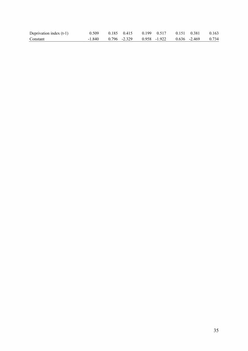
35
Deprivation index (t-1) 0.509 0.185 0.415 0.199 0.517 0.151 0.381 0.163Constant -1.840 0.796 -2.329 0.958 -1.922 0.636 -2.469 0.734