Mario Game Solver

Master Thesis

by

Kim Adelhardt and Nedyalko Kargov CPR: 240367-0025 CPR: 170982-4089 Email: kna1@itu.dk Email: nvka@itu.dk

Supervisors:

Kiniry, Joseph Roland Togelius, Julian

2

Table of contents Abstract...................................................................................................................................... 3

1. Background ............................................................................................................................ 4

1.1 Procedural Content Generation (PCG) ............................................................................. 4

1.2 Proof Carrying Code (PCC) .............................................................................................. 5

1.3 The Mario Solver .............................................................................................................. 6

2. Research question ................................................................................................................. 8

3. Research methods and techniques ........................................................................................ 9

3.1 Research methods ........................................................................................................... 9

3.2 Defining the Safety Policy ................................................................................................. 9

3.3 Defining the Model ............................................................................................................ 9

3.4 Defining the Prover ..........................................................................................................13

4. The Result.............................................................................................................................14

4.1 The Solver Implementation ..............................................................................................14

4.1.1 Basic Data Flow ........................................................................................................15

4.2 The algorithm...................................................................................................................22

4.2.1 Graph generation ......................................................................................................22

4.2.2 Graph analysis ..........................................................................................................24

4.2.3 Graph-depth - how deep can you go .........................................................................27

4.3 Algorithm Limitations ........................................................................................................30

4.4 Performance ....................................................................................................................30

5. Discussion ............................................................................................................................32

5.1 The Granularity of the logic ..............................................................................................32

5.2 The Mario Solver and the A* agent ..................................................................................34

5.3 Expanding the solution ....................................................................................................36

5.3.1 Expanding the Mario-alphabet ...................................................................................36

5.3.2 Extending the game characteristics and the step size ...............................................39

5.3.3 Extending the number of Mario actions .....................................................................41

5.4 Using different techniques ...............................................................................................42

5.4.1 SMT-LIB solver .........................................................................................................42

5.4.2 Different algorithm .....................................................................................................43

5.4.3 Optimized path ..........................................................................................................45

6. Conclusion ............................................................................................................................46

References ...............................................................................................................................47

Appendix ...................................................................................................................................49

The attached CD ...................................................................................................................49

List of videos ......................................................................................................................49

Equivalent classes and Level Configurations .........................................................................50

3

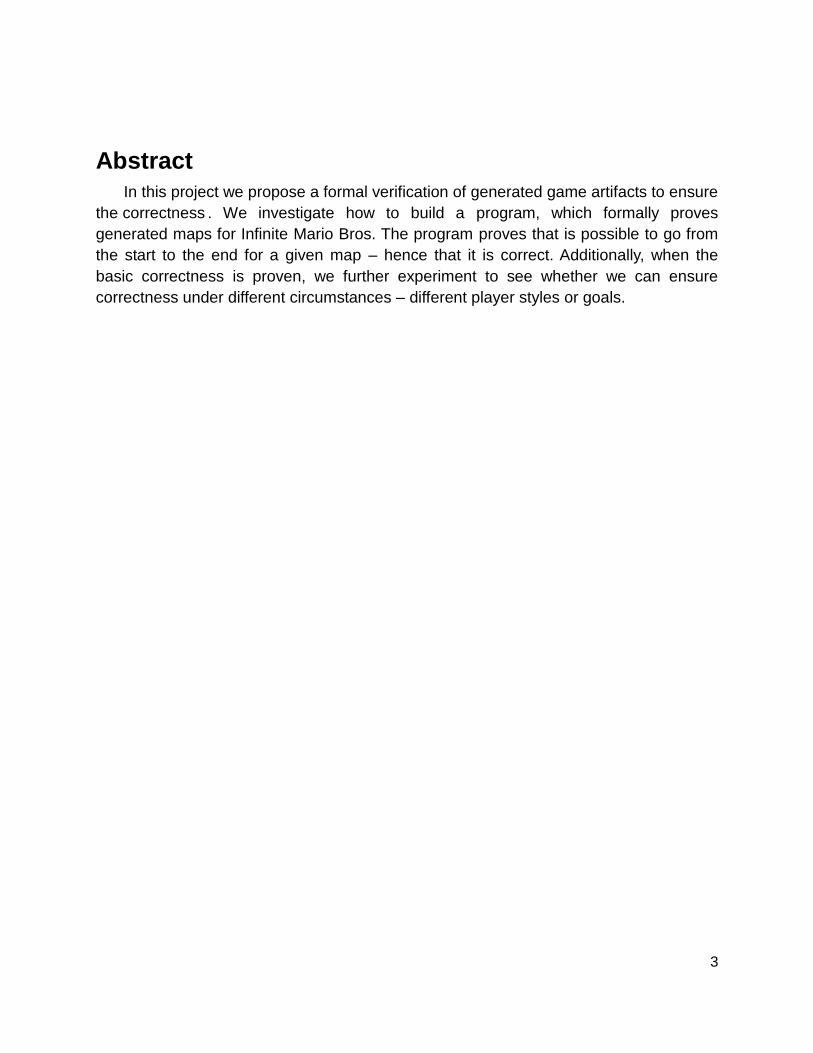
Abstract

In this project we propose a formal verification of generated game artifacts to ensure

the correctness . We investigate how to build a program, which formally proves

generated maps for Infinite Mario Bros. The program proves that is possible to go from

the start to the end for a given map – hence that it is correct. Additionally, when the

basic correctness is proven, we further experiment to see whether we can ensure

correctness under different circumstances – different player styles or goals.

4

1. Background

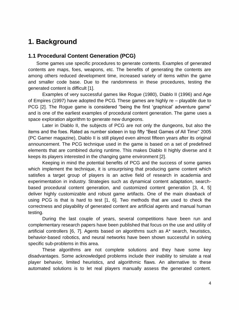
1.1 Procedural Content Generation (PCG)

Some games use specific procedures to generate contents. Examples of generated

contents are maps, foes, weapons, etc. The benefits of generating the contents are

among others reduced development time, increased variety of items within the game

and smaller code base. Due to the randomness in these procedures, testing the

generated content is difficult [1].

Examples of very successful games like Rogue (1980), Diablo II (1996) and Age

of Empires (1997) have adopted the PCG. These games are highly re – playable due to

PCG [2]. The Rogue game is considered “being the first ‘graphical’ adventure game”

and is one of the earliest examples of procedural content generation. The game uses a

space exploration algorithm to generate new dungeons.

Later in Diablo II, the subjects of PCG are not only the dungeons, but also the

items and the foes. Rated as number sixteen in top fifty “Best Games of All Time" 2005

(PC Gamer magazine), Diablo II is still played even almost fifteen years after its original

announcement. The PCG technique used in the game is based on a set of predefined

elements that are combined during runtime. This makes Diablo II highly diverse and it

keeps its players interested in the changing game environment [2].

Keeping in mind the potential benefits of PCG and the success of some games

which implement the technique, it is unsurprising that producing game content which

satisfies a target group of players is an active field of research in academia and

experimentation in industry. Strategies such as dynamical content adaptation, search-

based procedural content generation, and customized content generation [3, 4, 5]

deliver highly customizable and robust game artifacts. One of the main drawback of

using PCG is that is hard to test [1, 6]. Two methods that are used to check the

correctness and playability of generated content are artificial agents and manual human

testing.

During the last couple of years, several competitions have been run and

complementary research papers have been published that focus on the use and utility of

artificial controllers [6, 7]. Agents based on algorithms such as A* search, heuristics,

behavior-based robotics, and neural networks have been shown successful in solving

specific sub-problems in this area.

These algorithms are not complete solutions and they have some key

disadvantages. Some acknowledged problems include their inability to simulate a real

player behavior, limited heuristics, and algorithmic flaws. An alternative to these

automated solutions is to let real players manually assess the generated content.

5

Unfortunately, this is often expensive and does not scale, and is not an option for many

games [1].

Our work, summarized in this report, proposes a new, different way of

automatically evaluating generated content. To automatically check properties of

generated game content our proposed solution, embodied in our Mario Game Solver,

reinterprets generated game artifacts as a kind of program code with rich semantics,

rather than meaningless data. Practically, to demonstrate our approach, we focus on the

Infinite Mario Bros game—a free, Open Source clone of the original Mario Bros game

that is used for research and teaching in the area of PCG

1.2 Proof Carrying Code (PCC)

Over the last several decades formal verification has been applied to many

domains such as cryptographic protocols, digital circuits, and software correctness.

Formal verification focuses on logical reasoning about mathematical models of

hardware, software, and protocols using logic, resulting in the creation of formal proofs.

These proofs are evidence that a given system definitely has, or does not have, some

property of interest—for example, a CPU performs arithmetic correctly, a parallel

algorithm never deadlocks, or a piece of software never crashes.

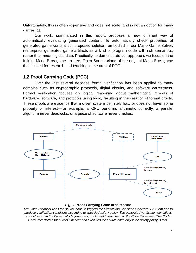
Fig. 1 Proof Carrying Code architecture

The Code Producer uses the source code to triggers the Verification Condition Generator (VCGen) and to produce verification conditions according to specified safety policy. The generated verification conditions are delivered to the Prover which generates proofs and hands them to the Code Consumer. The Code

Consumer uses a fast Proof Checker and executes the source code only if the safety policy is met.

6

In addition to the theoretical knowledge for formal verification some practical

implementations are made. The research investigates the Proof Carrying Code (PCC)

technique that allows establishment of trusted relationship between code producers and

code consumers. The responsibility of the code consumer is to provide a safety policy,

which specifies under what conditions it considers the execution of a program to be

safe. The responsibility of the code producer is to generate formal safety proofs. At the

end of the process the code consumer uses fast and simple validation to check that the

supplied proofs comply with the safety policy. Fig. 1 shows a brief overview of the Proof

Carrying Code architecture [9].

1.3 The Mario Solver

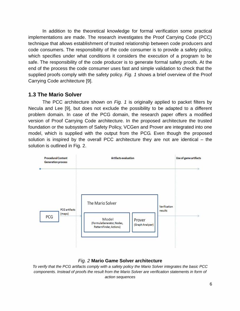
The PCC architecture shown on Fig. 1 is originally applied to packet filters by

Necula and Lee [9], but does not exclude the possibility to be adapted to a different

problem domain. In case of the PCG domain, the research paper offers a modified

version of Proof Carrying Code architecture. In the proposed architecture the trusted

foundation or the subsystem of Safety Policy, VCGen and Prover are integrated into one

model, which is supplied with the output from the PCG. Even though the proposed

solution is inspired by the overall PCC architecture they are not are identical – the

solution is outlined in Fig. 2.

Fig. 2 Mario Game Solver architecture

To verify that the PCG artifacts comply with a safety policy the Mario Solver integrates the basic PCC

components. Instead of proofs the result from the Mario Solver are verification statements in form of

action sequences

7

Given a map, the Mario Solver generates a sequence of coordinates describing a path. The

path is seen as a proof of playability, if it is possible to traverse the path from the start to a win.

The correctness of the solution is based on the implemented algorithm. Hence it is vital that the

algorithm is suited for the task and that it is implemented accurately. The implementation is

presented in the report as pseudo code and are discussed in section 4.2 The algorithm

8

2. Research question “Is it possible to build an application based on PCC-techniques that can declare certain procedurally generated maps playable?”

Concrete goals: Main goal:

1. Prove that certain PCG maps for Infinite Mario Bros are playable in terms

of the possibility to traverse the level from the beginning to the end.

Secondary goals:

1. Find the shortest path from the start to a win.

2. Prove the playability of the level without doing any long jumps.

Optional goals:

1. Find the successful winning strategy which gives you most coins collected. 2. Find the successful winning strategy which gives you most enemies killed.

The research question and the specific goals are formulated with two major factors

in mind. The auto generated maps must be proven to be playable, the performance of

the actual solution should be realistic in terms of time and memory consumption and the

solver should be capable of answering variety of additional questions.

The reason for defining such restrictions to the proposed solution is that, even

though the theoretical value of the research can have certain effect on the academia, a

better result would be to solve real world problems and see in practice how a different

approach could benefit the industry. By building the solution with expansion in mind, we

hope to encourage others to continue the research.

9

3. Research methods and techniques

The current section of the report formally defines the research methods, explains

what is considered to be a safety policy and what constitutes safe code behavior. Later

the basic principles behind the solution design are explained.

3.1 Research methods

Due to the research question and the investigational nature of the project the

flexible experimental research type is chosen. The project experiments with the code.

The first working prototype is regarded as the baseline. All further experiments compare

time, size and memory consumption as goals for improvements.

3.2 Defining the Safety Policy

The game artifacts subject of PCG may vary by type, but all of them have to

comply with specific requirements. The restrictions put on weapons, maps, game

characters, etc. are all different, but none of them must compromise the game integrity

or the overall architecture. In the current solution the safety policies are defined as:

The PCG maps (the game artifact used in the report) must be playable. In more

concrete sense: the level should be constructed in a way so that it is possible to

reach the finish line within the allotted time.

This general rule is broken down into a set of formal rules by analyzing the game.

These rules are used as a foundation to build a model of the game. The rules are used

as axioms in the solver.

3.3 Defining the Model

Even though the real game is characterized with great variety of elements and

rules, the research includes only a limited number of game entities. The limitation is

done for the purpose of simplicity and to make a proof of concept. The idea behind the

game element selection is to find categories of elements, with similar properties and

select only these, which will be representative for a specific category.

After making a list of the game elements involved in the Infinite Mario Bros

gameplay, the following are chosen to be representative and are used in the following

research.

10

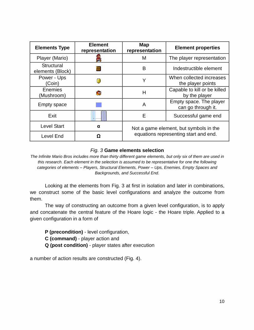
Elements Type Element

representation Map

representation Element properties

Player (Mario)

M The player representation

Structural elements (Block) B Indestructible element

Power - Ups (Coin) Y

When collected increases the player points

Enemies (Mushroom) H

Capable to kill or be killed by the player

Empty space A Empty space. The player

can go through it.

Exit

E Successful game end

Level Start α Not a game element, but symbols in the equations representing start and end. Level End Ω

Fig. 3 Game elements selection

The Infinite Mario Bros includes more than thirty different game elements, but only six of them are used in

this research. Each element in the selection is assumed to be representative for one the following

categories of elements – Players, Structural Elements, Power – Ups, Enemies, Empty Spaces and

Backgrounds, and Successful End.

Looking at the elements from Fig. 3 at first in isolation and later in combinations,

we construct some of the basic level configurations and analyze the outcome from

them.

The way of constructing an outcome from a given level configuration, is to apply

and concatenate the central feature of the Hoare logic - the Hoare triple. Applied to a

given configuration in a form of

P (precondition) - level configuration,

C (command) - player action and

Q (post condition) - player states after execution

a number of action results are constructed (Fig. 4).

11

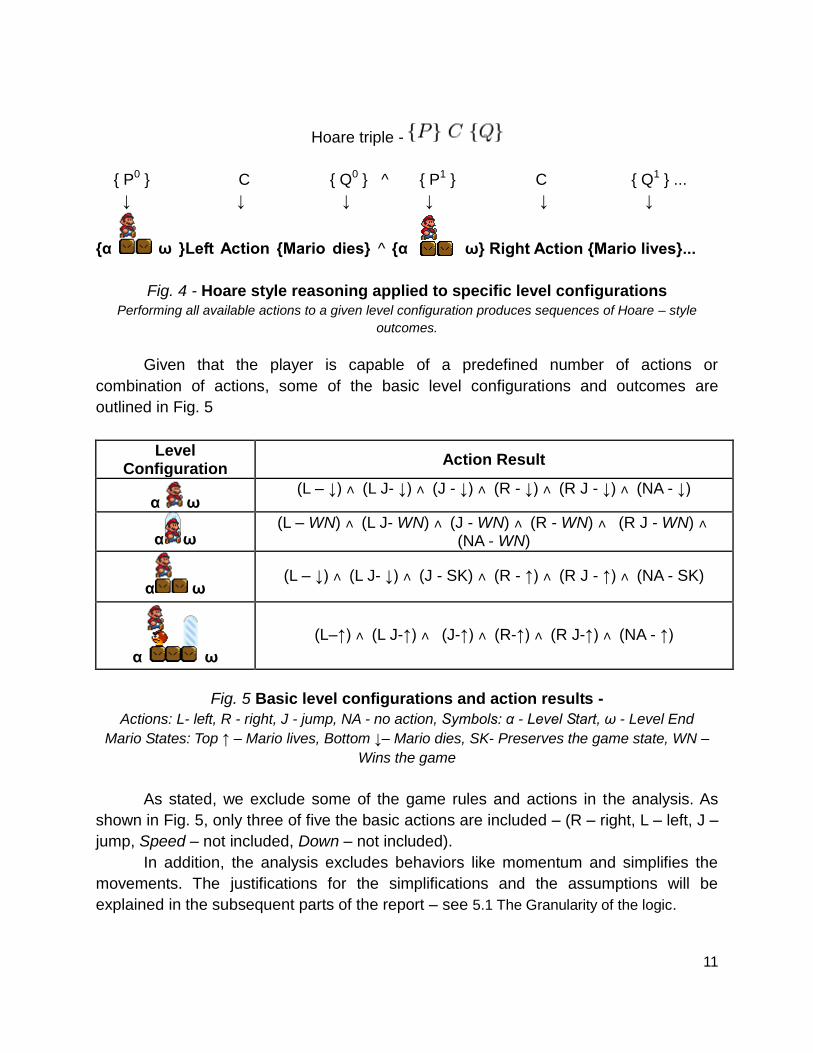
Hoare triple -

{ P0 } C { Q0 } ^ { P1 } C { Q1 } ...

↓ ↓ ↓ ↓ ↓ ↓

{α ω }Left Action {Mario dies} ^ {α ω} Right Action {Mario lives}...

Fig. 4 - Hoare style reasoning applied to specific level configurations

Performing all available actions to a given level configuration produces sequences of Hoare – style

outcomes.

Given that the player is capable of a predefined number of actions or

combination of actions, some of the basic level configurations and outcomes are

outlined in Fig. 5

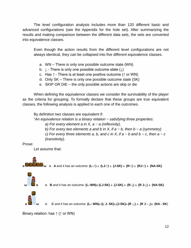
Level Configuration

Action Result

α ω (L – ↓) ˄ (L J- ↓) ˄ (J - ↓) ˄ (R - ↓) ˄ (R J - ↓) ˄ (NA - ↓)

α ω (L – WN) ˄ (L J- WN) ˄ (J - WN) ˄ (R - WN) ˄ (R J - WN) ˄

(NA - WN)

α ω (L – ↓) ˄ (L J- ↓) ˄ (J - SK) ˄ (R - ↑) ˄ (R J - ↑) ˄ (NA - SK)

α ω

(L–↑) ˄ (L J-↑) ˄ (J-↑) ˄ (R-↑) ˄ (R J-↑) ˄ (NA - ↑)

Fig. 5 Basic level configurations and action results -

Actions: L- left, R - right, J - jump, NA - no action, Symbols: α - Level Start, ω - Level End

Mario States: Top ↑ – Mario lives, Bottom ↓– Mario dies, SK- Preserves the game state, WN –

Wins the game

As stated, we exclude some of the game rules and actions in the analysis. As

shown in Fig. 5, only three of five the basic actions are included – (R – right, L – left, J –

jump, Speed – not included, Down – not included).

In addition, the analysis excludes behaviors like momentum and simplifies the

movements. The justifications for the simplifications and the assumptions will be

explained in the subsequent parts of the report – see 5.1 The Granularity of the logic.

12

The level configuration analysis includes more than 120 different basic and

advanced configurations (see the Appendix for the hole set). After summarizing the

results and making comparison between the different data sets, the sets are converted

into equivalence classes.

Even though the action results from the different level configurations are not

always identical, they can be collapsed into five different equivalence classes.

a. WN – There is only one possible outcome state (WN)

b. ↓ - There is only one possible outcome state (↓)

c. Has ↑ - There is at least one positive outcome (↑ or WN)

d. Only SK – There is only one possible outcome state (SK)

e. SKIP OR DIE – the only possible actions are skip or die

When defining the equivalence classes we consider the survivability of the player

as the criteria for grouping. To formally declare that these groups are true equivalent

classes, the following analysis is applied to each one of the outcomes.

By definition two classes are equivalent if:

“An equivalence relation is a binary relation ~ satisfying three properties:

a) For every element a in X, a ~ a (reflexivity),

b) For every two elements a and b in X, if a ~ b, then b ~ a (symmetry)

c) For every three elements a, b, and c in X, if a ~ b and b ~ c, then a ~ c

(transitivity).

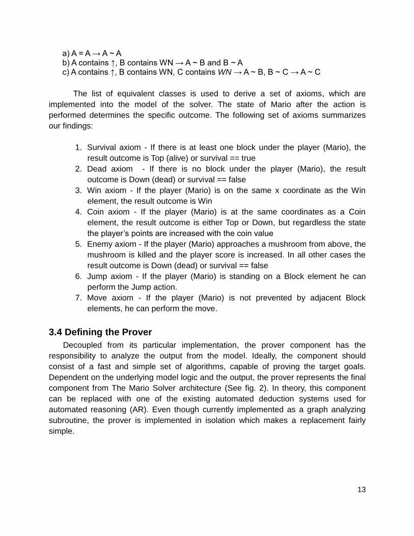
Prove:

Let assume that:

α ω is A and it has an outcome: (L–↑) ˄ (LJ-↑) ˄ (J-SK) ˄ (R-↑) ˄ (RJ-↑) ˄ (NA-SK)

ω α is B and it has an outcome: (L–WN)˄ (LJ-SK) ˄ (J-SK) ˄ (R-↓) ˄ (R J-↓) ˄ (NA-SK)

α ω is C and it has an outcome: (L– WN)˄ (L J- SK)˄ (J-SK)˄ (R -↓) ˄ (R J - ↓)˄ (NA - SK)

Binary relation: has ↑ (↑ or WN)

13

a) A = A → A ~ A b) A contains ↑, B contains WN → A ~ B and B ~ A c) A contains ↑, B contains WN, C contains WN → A ~ B, B ~ C → A ~ C

The list of equivalent classes is used to derive a set of axioms, which are

implemented into the model of the solver. The state of Mario after the action is

performed determines the specific outcome. The following set of axioms summarizes

our findings:

1. Survival axiom - If there is at least one block under the player (Mario), the

result outcome is Top (alive) or survival == true

2. Dead axiom - If there is no block under the player (Mario), the result

outcome is Down (dead) or survival == false

3. Win axiom - If the player (Mario) is on the same x coordinate as the Win

element, the result outcome is Win

4. Coin axiom - If the player (Mario) is at the same coordinates as a Coin

element, the result outcome is either Top or Down, but regardless the state

the player’s points are increased with the coin value

5. Enemy axiom - If the player (Mario) approaches a mushroom from above, the

mushroom is killed and the player score is increased. In all other cases the

result outcome is Down (dead) or survival == false

6. Jump axiom - If the player (Mario) is standing on a Block element he can

perform the Jump action.

7. Move axiom - If the player (Mario) is not prevented by adjacent Block

elements, he can perform the move.

3.4 Defining the Prover

Decoupled from its particular implementation, the prover component has the

responsibility to analyze the output from the model. Ideally, the component should

consist of a fast and simple set of algorithms, capable of proving the target goals.

Dependent on the underlying model logic and the output, the prover represents the final

component from The Mario Solver architecture (See fig. 2). In theory, this component

can be replaced with one of the existing automated deduction systems used for

automated reasoning (AR). Even though currently implemented as a graph analyzing

subroutine, the prover is implemented in isolation which makes a replacement fairly

simple.

14

4. The Result

This section of the report covers three parts – the solver implementation, the

Algorithm and the Performance results.

4.1 The Solver Implementation

The Infinite Mario Bros (Markus Persson, 2008) is an open source Java

implementation of the classic platform game Super Mario Bros (1985). The game is

playable online and the Java source code is available for download. In the current

research project we use a modified version of the Infinite Mario Bros. This version of the

game is used in “The Mario AI Competition 2009” organized by Julian Togelius, Sergey

Karakovskiy and Noor Shaker. In addition, we also integrate with a customized version

of the same game provided by Robin Baumgarten. His version is equipped with his A*

agent (A* following mouse) implementation.

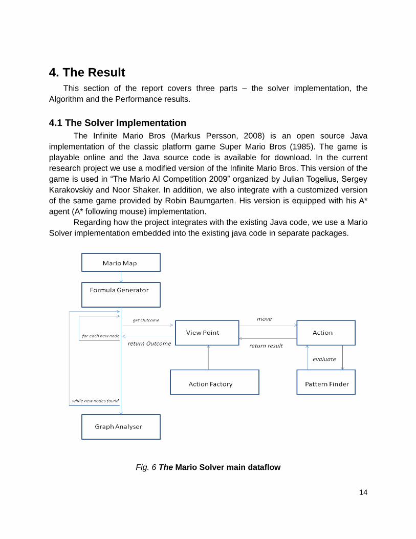
Regarding how the project integrates with the existing Java code, we use a Mario

Solver implementation embedded into the existing java code in separate packages.

Fig. 6 The Mario Solver main dataflow

15

The solver has the following capabilities:

Covers only one Mario mode – small.

Performs seven actions –(R – Right, L – Left, J – Jump, RJ – Right + Jump,

LJ – Left + Jump, JR – Jump + Right, JL – Jump + Left )

Includes only one kind of enemy (mushroom)

Excludes weapons – Mario cannot shoot

Keeps the height of the jumps / step size constant.

Defines the length of the step from the beginning of the block to the

beginning of the adjacent block – in the real game, this normally consists

of sixteen individual steps.

Operates on game elements mentioned in Fig 3 - Game elements selection

The time for step is constant

The time for jump is constant

Only one life

4.1.1 Basic Data Flow

The basic dataflow presented in Fig. 6 shows the main set of components involved

in the Mario Solver implementation. Even though the dataflow is not a complete picture,

the following components are forming the base of the Mario Solver and they are

explained.

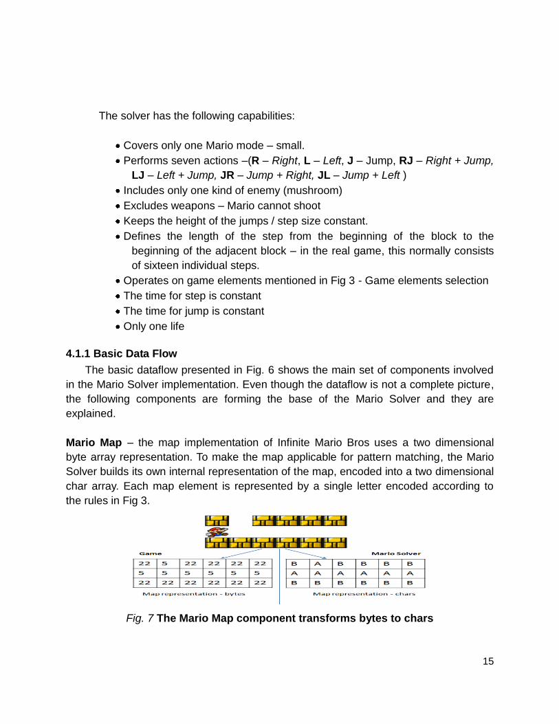
Mario Map – the map implementation of Infinite Mario Bros uses a two dimensional

byte array representation. To make the map applicable for pattern matching, the Mario

Solver builds its own internal representation of the map, encoded into a two dimensional

char array. Each map element is represented by a single letter encoded according to

the rules in Fig 3.

Fig. 7 The Mario Map component transforms bytes to chars

16

Formula Generator - this element has the responsibility to construct a graph

representation of the visited nodes. The Formula Generator is the component which

implements the main algorithm loop and also builds the graph according to the

algorithm restrictions (see Graph-depth - how deep can you go). The algorithm used is

a BFS.

In the first experiments the algorithm was implemented using recursive method

calls. Later, the generator was changed to use only iterations. The reason for changing

the implementation was, that even though the recursive calls certainly show the power

of computing, the implementation is memory demanding and opens the door for a

potential stack overflow.

In pseudo code:

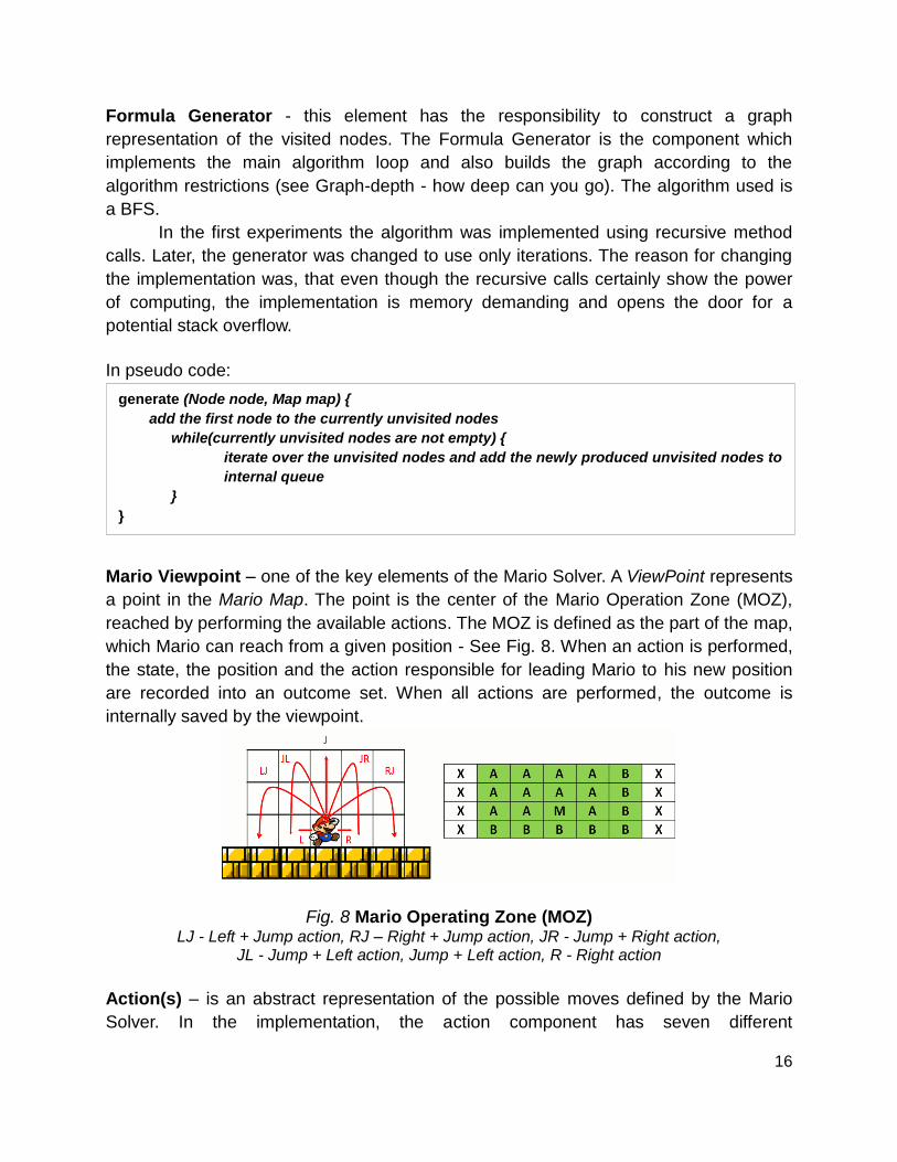
Mario Viewpoint – one of the key elements of the Mario Solver. A ViewPoint represents

a point in the Mario Map. The point is the center of the Mario Operation Zone (MOZ),

reached by performing the available actions. The MOZ is defined as the part of the map,

which Mario can reach from a given position - See Fig. 8. When an action is performed,

the state, the position and the action responsible for leading Mario to his new position

are recorded into an outcome set. When all actions are performed, the outcome is

internally saved by the viewpoint.

Fig. 8 Mario Operating Zone (MOZ)

LJ - Left + Jump action, RJ – Right + Jump action, JR - Jump + Right action, JL - Jump + Left action, Jump + Left action, R - Right action

Action(s) – is an abstract representation of the possible moves defined by the Mario

Solver. In the implementation, the action component has seven different

generate (Node node, Map map) {

add the first node to the currently unvisited nodes

while(currently unvisited nodes are not empty) {

iterate over the unvisited nodes and add the newly produced unvisited nodes to

internal queue

}

}

17

implementations - each one representing a different action or combination of actions.

Each implementation has its own rules and restrictions. Some of the rules define

movement mechanics (how high is the jump, how much time does it takes to perform

the action, etc.). Other rules describe the process of killing enemies or how to move for

collecting coins.

The action rules are implemented based on the already defined game axioms.

The axioms are found during the analysis phase of the research. Each action applies

these rules in horizontal and vertical way by interacting with the Pattern Finder

component discussed later in the report. Before saving the new node (or viewpoint) in

the outcome, gravity is applied. In addition, statistical information regarding the collected

coins and killed enemies are recorded. To ease the understanding on how the separate

actions are implemented and performed, some representative actions are outlined in the

following sections.

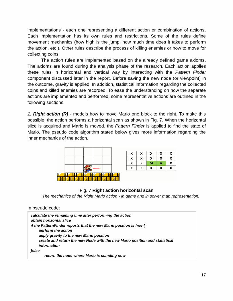
1. Right action (R) - models how to move Mario one block to the right. To make this

possible, the action performs a horizontal scan as shown in Fig. 7. When the horizontal

slice is acquired and Mario is moved, the Pattern Finder is applied to find the state of

Mario. The pseudo code algorithm stated below gives more information regarding the

inner mechanics of the action.

Fig. 7 Right action horizontal scan

The mechanics of the Right Mario action - in game and in solver map representation.

In pseudo code:

calculate the remaining time after performing the action

obtain horizontal slice

if the PatternFinder reports that the new Mario position is free {

perform the action

apply gravity to the new Mario position

create and return the new Node with the new Mario position and statistical

information

}else

return the node where Mario is standing now

18

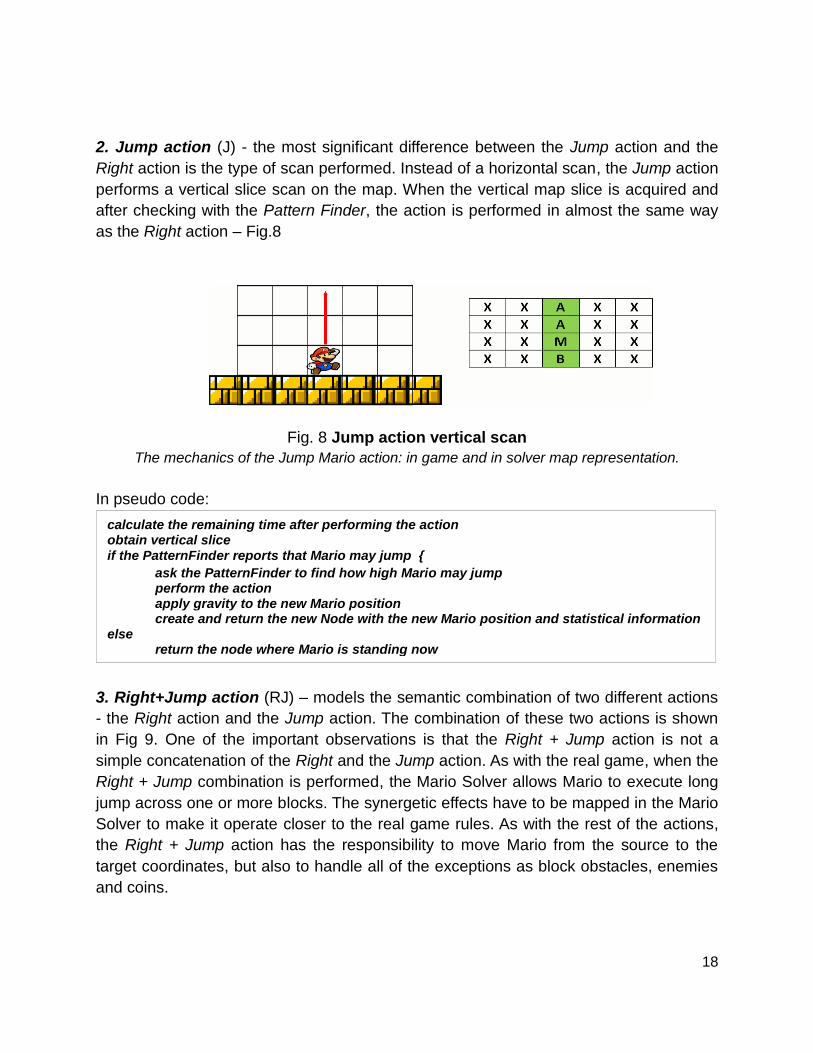
2. Jump action (J) - the most significant difference between the Jump action and the

Right action is the type of scan performed. Instead of a horizontal scan, the Jump action

performs a vertical slice scan on the map. When the vertical map slice is acquired and

after checking with the Pattern Finder, the action is performed in almost the same way

as the Right action – Fig.8

Fig. 8 Jump action vertical scan

The mechanics of the Jump Mario action: in game and in solver map representation.

In pseudo code:

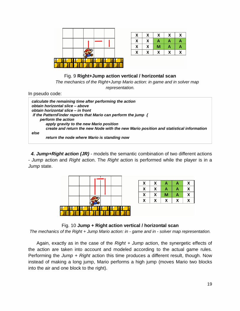
3. Right+Jump action (RJ) – models the semantic combination of two different actions

- the Right action and the Jump action. The combination of these two actions is shown

in Fig 9. One of the important observations is that the Right + Jump action is not a

simple concatenation of the Right and the Jump action. As with the real game, when the

Right + Jump combination is performed, the Mario Solver allows Mario to execute long

jump across one or more blocks. The synergetic effects have to be mapped in the Mario

Solver to make it operate closer to the real game rules. As with the rest of the actions,

the Right + Jump action has the responsibility to move Mario from the source to the

target coordinates, but also to handle all of the exceptions as block obstacles, enemies

and coins.

calculate the remaining time after performing the action obtain vertical slice if the PatternFinder reports that Mario may jump {

ask the PatternFinder to find how high Mario may jump perform the action apply gravity to the new Mario position create and return the new Node with the new Mario position and statistical information

else return the node where Mario is standing now

19

Fig. 9 Right+Jump action vertical / horizontal scan

The mechanics of the Right+Jump Mario action: in game and in solver map

representation.

In pseudo code:

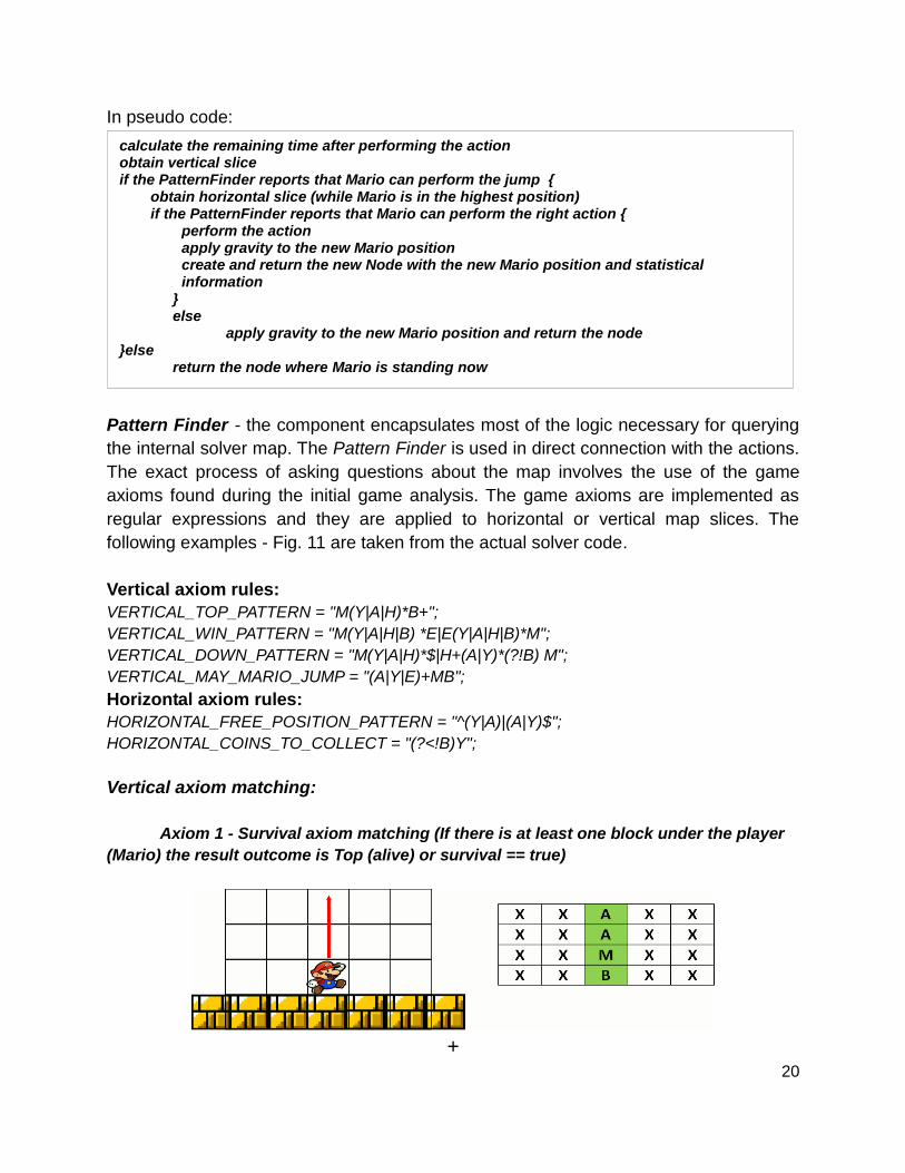
4. Jump+Right action (JR) - models the semantic combination of two different actions

- Jump action and Right action. The Right action is performed while the player is in a

Jump state.

Fig. 10 Jump + Right action vertical / horizontal scan

The mechanics of the Right + Jump Mario action: in - game and in - solver map representation.

Again, exactly as in the case of the Right + Jump action, the synergetic effects of

the action are taken into account and modeled according to the actual game rules.

Performing the Jump + Right action this time produces a different result, though. Now

instead of making a long jump, Mario performs a high jump (moves Mario two blocks

into the air and one block to the right).

calculate the remaining time after performing the action obtain horizontal slice – above obtain horizontal slice – in front if the PatternFinder reports that Mario can perform the jump { perform the action

apply gravity to the new Mario position create and return the new Node with the new Mario position and statistical information

else return the node where Mario is standing now

20

In pseudo code:

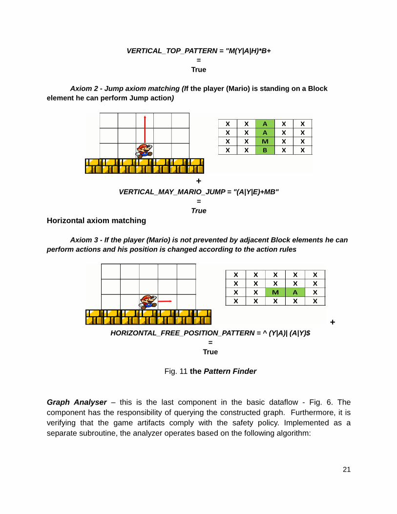
Pattern Finder - the component encapsulates most of the logic necessary for querying

the internal solver map. The Pattern Finder is used in direct connection with the actions.

The exact process of asking questions about the map involves the use of the game

axioms found during the initial game analysis. The game axioms are implemented as

regular expressions and they are applied to horizontal or vertical map slices. The

following examples - Fig. 11 are taken from the actual solver code.

Vertical axiom rules:

VERTICAL_TOP_PATTERN = "M(Y|A|H)*B+";

VERTICAL_WIN_PATTERN = "M(Y|A|H|B) *E|E(Y|A|H|B)*M";

VERTICAL_DOWN_PATTERN = "M(Y|A|H)*$|H+(A|Y)*(?!B) M";

VERTICAL_MAY_MARIO_JUMP = "(A|Y|E)+MB";

Horizontal axiom rules:

HORIZONTAL_FREE_POSITION_PATTERN = "^(Y|A)|(A|Y)$";

HORIZONTAL_COINS_TO_COLLECT = "(?<!B)Y";

Vertical axiom matching:

Axiom 1 - Survival axiom matching (If there is at least one block under the player

(Mario) the result outcome is Top (alive) or survival == true)

+

calculate the remaining time after performing the action obtain vertical slice if the PatternFinder reports that Mario can perform the jump { obtain horizontal slice (while Mario is in the highest position) if the PatternFinder reports that Mario can perform the right action { perform the action

apply gravity to the new Mario position create and return the new Node with the new Mario position and statistical information

} else

apply gravity to the new Mario position and return the node }else

return the node where Mario is standing now

21

VERTICAL_TOP_PATTERN = "M(Y|A|H)*B+

=

True

Axiom 2 - Jump axiom matching (If the player (Mario) is standing on a Block

element he can perform Jump action)

+

VERTICAL_MAY_MARIO_JUMP = "(A|Y|E)+MB"

=

True

Horizontal axiom matching

Axiom 3 - If the player (Mario) is not prevented by adjacent Block elements he can

perform actions and his position is changed according to the action rules

+ HORIZONTAL_FREE_POSITION_PATTERN = ^ (Y|A)| (A|Y)$

=

True

Fig. 11 the Pattern Finder

Graph Analyser – this is the last component in the basic dataflow - Fig. 6. The

component has the responsibility of querying the constructed graph. Furthermore, it is

verifying that the game artifacts comply with the safety policy. Implemented as a

separate subroutine, the analyzer operates based on the following algorithm:

22

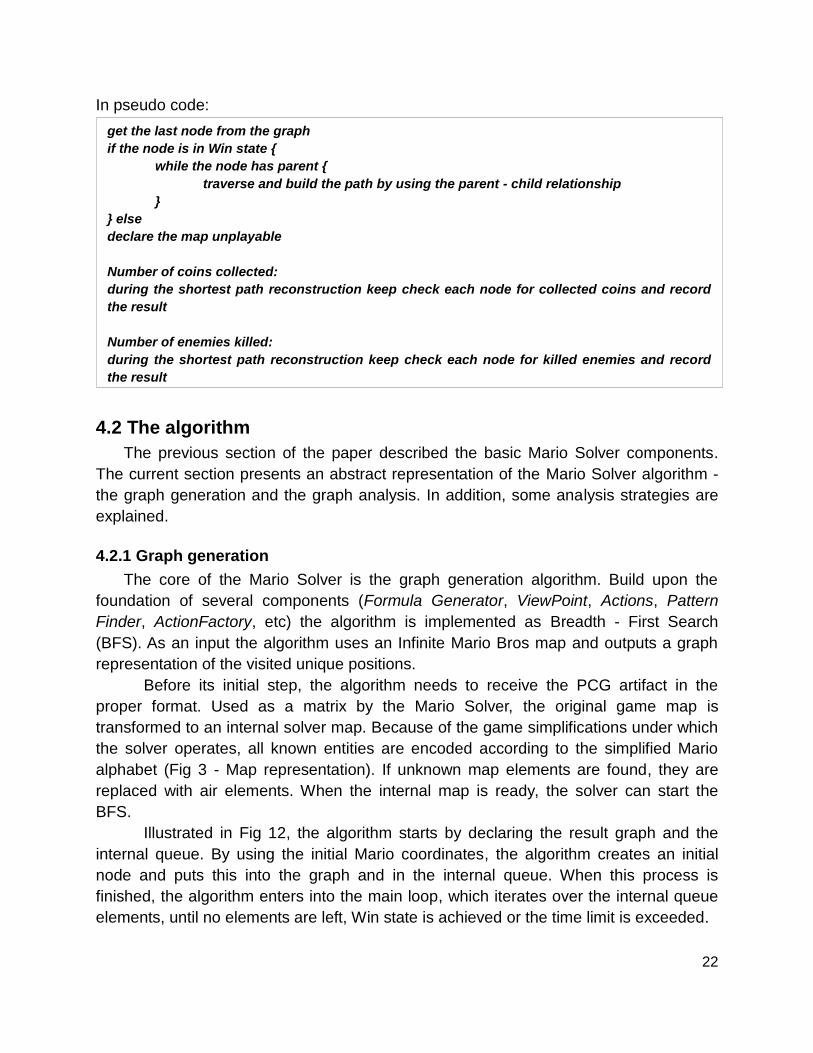
In pseudo code:

4.2 The algorithm

The previous section of the paper described the basic Mario Solver components.

The current section presents an abstract representation of the Mario Solver algorithm -

the graph generation and the graph analysis. In addition, some analysis strategies are

explained.

4.2.1 Graph generation

The core of the Mario Solver is the graph generation algorithm. Build upon the

foundation of several components (Formula Generator, ViewPoint, Actions, Pattern

Finder, ActionFactory, etc) the algorithm is implemented as Breadth - First Search

(BFS). As an input the algorithm uses an Infinite Mario Bros map and outputs a graph

representation of the visited unique positions.

Before its initial step, the algorithm needs to receive the PCG artifact in the

proper format. Used as a matrix by the Mario Solver, the original game map is

transformed to an internal solver map. Because of the game simplifications under which

the solver operates, all known entities are encoded according to the simplified Mario

alphabet (Fig 3 - Map representation). If unknown map elements are found, they are

replaced with air elements. When the internal map is ready, the solver can start the

BFS.

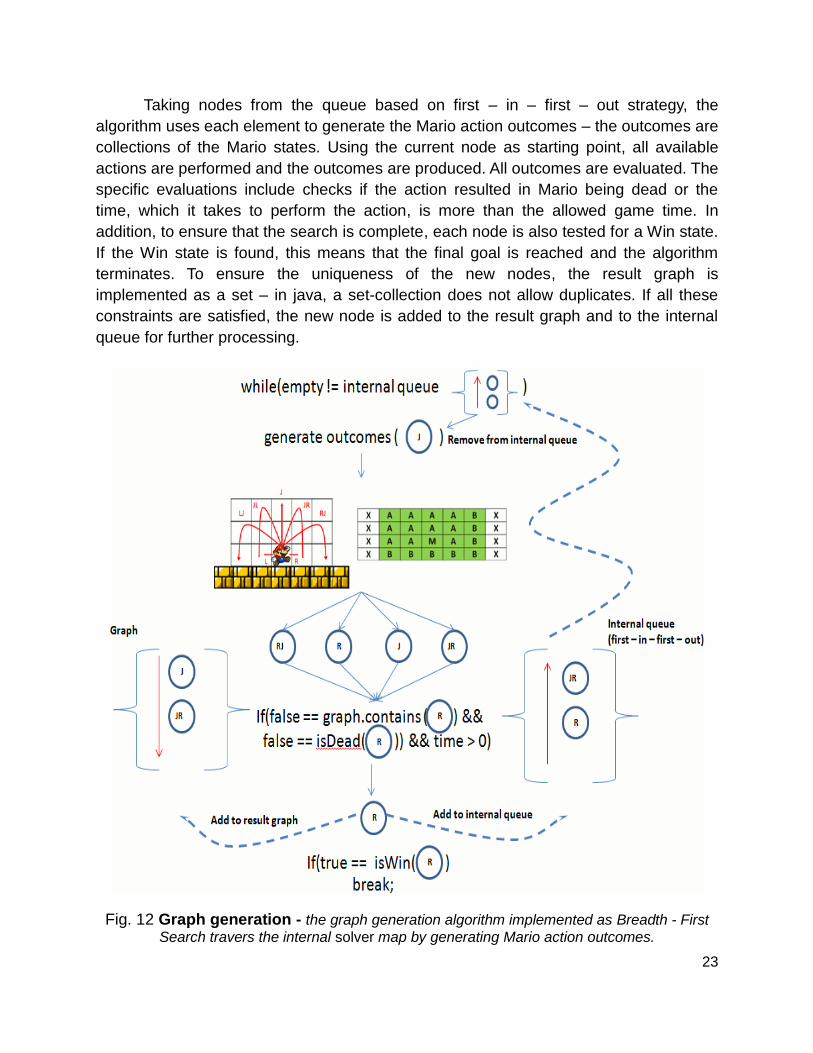
Illustrated in Fig 12, the algorithm starts by declaring the result graph and the

internal queue. By using the initial Mario coordinates, the algorithm creates an initial

node and puts this into the graph and in the internal queue. When this process is

finished, the algorithm enters into the main loop, which iterates over the internal queue

elements, until no elements are left, Win state is achieved or the time limit is exceeded.

get the last node from the graph

if the node is in Win state {

while the node has parent {

traverse and build the path by using the parent - child relationship

}

} else

declare the map unplayable

Number of coins collected:

during the shortest path reconstruction keep check each node for collected coins and record

the result

Number of enemies killed:

during the shortest path reconstruction keep check each node for killed enemies and record

the result

23

Taking nodes from the queue based on first – in – first – out strategy, the

algorithm uses each element to generate the Mario action outcomes – the outcomes are

collections of the Mario states. Using the current node as starting point, all available

actions are performed and the outcomes are produced. All outcomes are evaluated. The

specific evaluations include checks if the action resulted in Mario being dead or the

time, which it takes to perform the action, is more than the allowed game time. In

addition, to ensure that the search is complete, each node is also tested for a Win state.

If the Win state is found, this means that the final goal is reached and the algorithm

terminates. To ensure the uniqueness of the new nodes, the result graph is

implemented as a set – in java, a set-collection does not allow duplicates. If all these

constraints are satisfied, the new node is added to the result graph and to the internal

queue for further processing.

Fig. 12 Graph generation - the graph generation algorithm implemented as Breadth - First

Search travers the internal solver map by generating Mario action outcomes.

24

In pseudo code:

4.2.2 Graph analysis

In this section the analysis of the graph is broken down to three entry points – based

on the goals of the experiment

Pre-analysis

The increased interest towards digital media and games in the last couple of years

brought the attention of many researchers. Most of the time, in order to collect the

research data, they use artificial agents or human testers, to test and evaluate the

content [13, 14]. Unfortunately, not being able to simulate real human behavior or

because it is a labor intensive task, these two methods suffer from increased expenses

or incorrect data. This is covered in section 1.1 PCG.

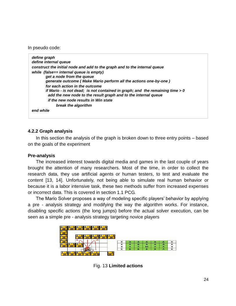
The Mario Solver proposes a way of modeling specific players’ behavior by applying

a pre - analysis strategy and modifying the way the algorithm works. For instance,

disabling specific actions (the long jumps) before the actual solver execution, can be

seen as a simple pre - analysis strategy targeting novice players

Fig. 13 Limited actions

define graph define internal queue

construct the initial node and add to the graph and to the internal queue

while (false== internal queue is empty) get a node from the queue generate outcome ( Make Mario perform all the actions one-by-one )

for each action in the outcome if Mario - is not dead; is not contained in graph; and the remaining time > 0

add the new node to the result graph and to the internal queue

if the new node results in Win state

break the algorithm

end while

25

The pre - analysis strategy modifies the work of the generator algorithm. In this case, the

algorithm models a novice player, which is not capable of performing long jumps. By removing

the long jumps from the available action, the solver needs to take the long path instead of

jumping across the obstacle.

Even though an experienced user can overcome the jump without considerable

efforts and finish the game on time, this small impediment could be the place where

most of the novice players fail. Frustrated and disappointed they might declare the map

unplayable.

By applying a pre - analysis strategy the graph can be generated with a specific

purpose and answer the concrete questions – see 5.4.2 Different algorithm.

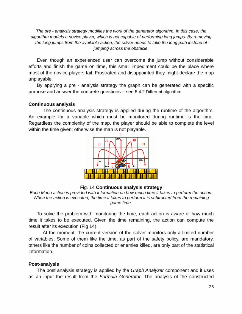
Continuous analysis

The continuous analysis strategy is applied during the runtime of the algorithm.

An example for a variable which must be monitored during runtime is the time.

Regardless the complexity of the map, the player should be able to complete the level

within the time given; otherwise the map is not playable.

Fig. 14 Continuous analysis strategy

Each Mario action is provided with information on how much time it takes to perform the action. When the action is executed, the time it takes to perform it is subtracted from the remaining

game time.

To solve the problem with monitoring the time, each action is aware of how much

time it takes to be executed. Given the time remaining, the action can compute the

result after its execution (Fig 14).

At the moment, the current version of the solver monitors only a limited number

of variables. Some of them like the time, as part of the safety policy, are mandatory,

others like the number of coins collected or enemies killed, are only part of the statistical

information.

Post-analysis

The post analysis strategy is applied by the Graph Analyzer component and it uses

as an input the result from the Formula Generator. The analysis of the constructed

26

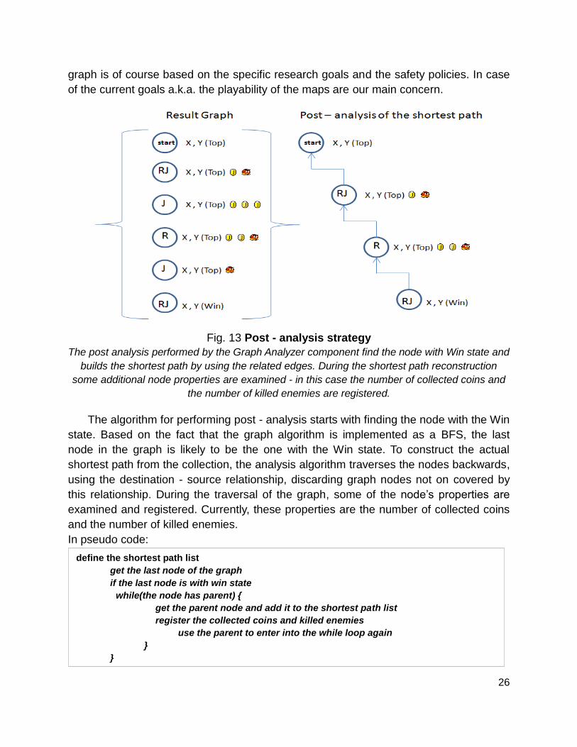
graph is of course based on the specific research goals and the safety policies. In case

of the current goals a.k.a. the playability of the maps are our main concern.

Fig. 13 Post - analysis strategy

The post analysis performed by the Graph Analyzer component find the node with Win state and

builds the shortest path by using the related edges. During the shortest path reconstruction

some additional node properties are examined - in this case the number of collected coins and

the number of killed enemies are registered.

The algorithm for performing post - analysis starts with finding the node with the Win

state. Based on the fact that the graph algorithm is implemented as a BFS, the last

node in the graph is likely to be the one with the Win state. To construct the actual

shortest path from the collection, the analysis algorithm traverses the nodes backwards,

using the destination - source relationship, discarding graph nodes not on covered by

this relationship. During the traversal of the graph, some of the node’s properties are

examined and registered. Currently, these properties are the number of collected coins

and the number of killed enemies.

In pseudo code:

define the shortest path list

get the last node of the graph

if the last node is with win state

while(the node has parent) {

get the parent node and add it to the shortest path list

register the collected coins and killed enemies

use the parent to enter into the while loop again

}

}

27

4.2.3 Graph-depth - how deep can you go

Constructed by the Formula Generator component with BFS, the internal graph

requires restrictions on its size. The restrictions are “only visiting nodes, not already

visited" and prevent the algorithm of running into endless loops or cycles [16]. That

leads to defining requirements of what exactly is an already visited node.

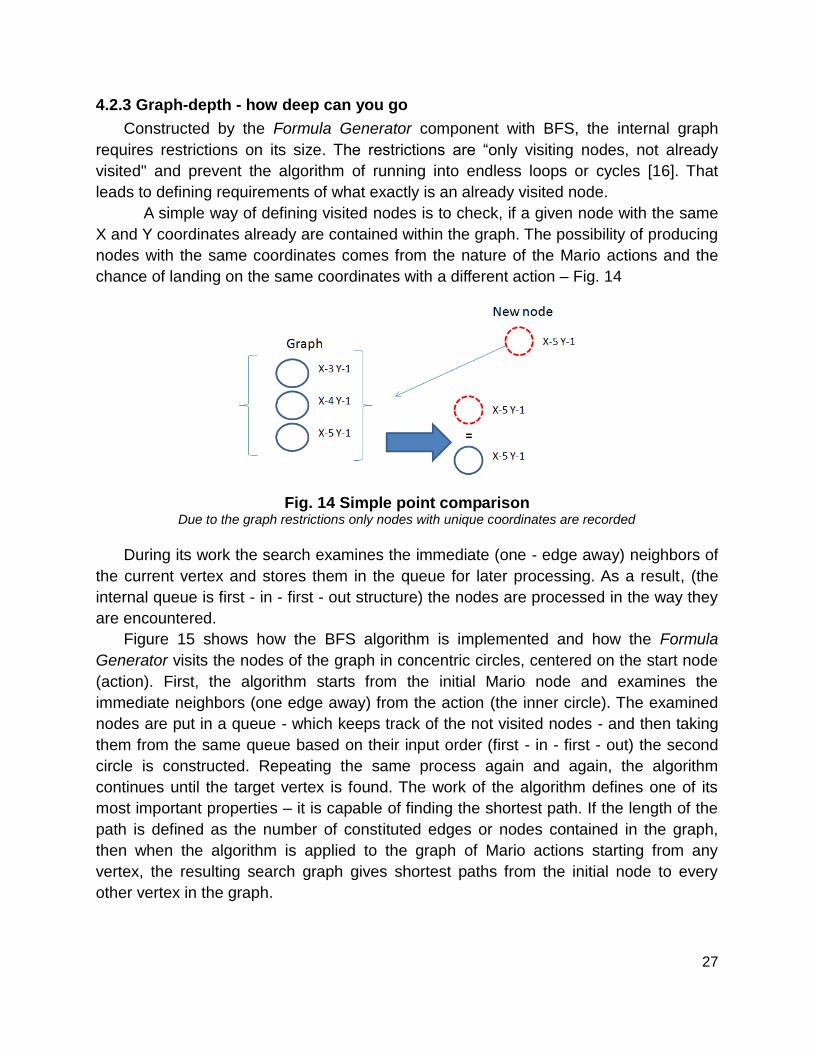
A simple way of defining visited nodes is to check, if a given node with the same

X and Y coordinates already are contained within the graph. The possibility of producing

nodes with the same coordinates comes from the nature of the Mario actions and the

chance of landing on the same coordinates with a different action – Fig. 14

Fig. 14 Simple point comparison Due to the graph restrictions only nodes with unique coordinates are recorded

During its work the search examines the immediate (one - edge away) neighbors of

the current vertex and stores them in the queue for later processing. As a result, (the

internal queue is first - in - first - out structure) the nodes are processed in the way they

are encountered.

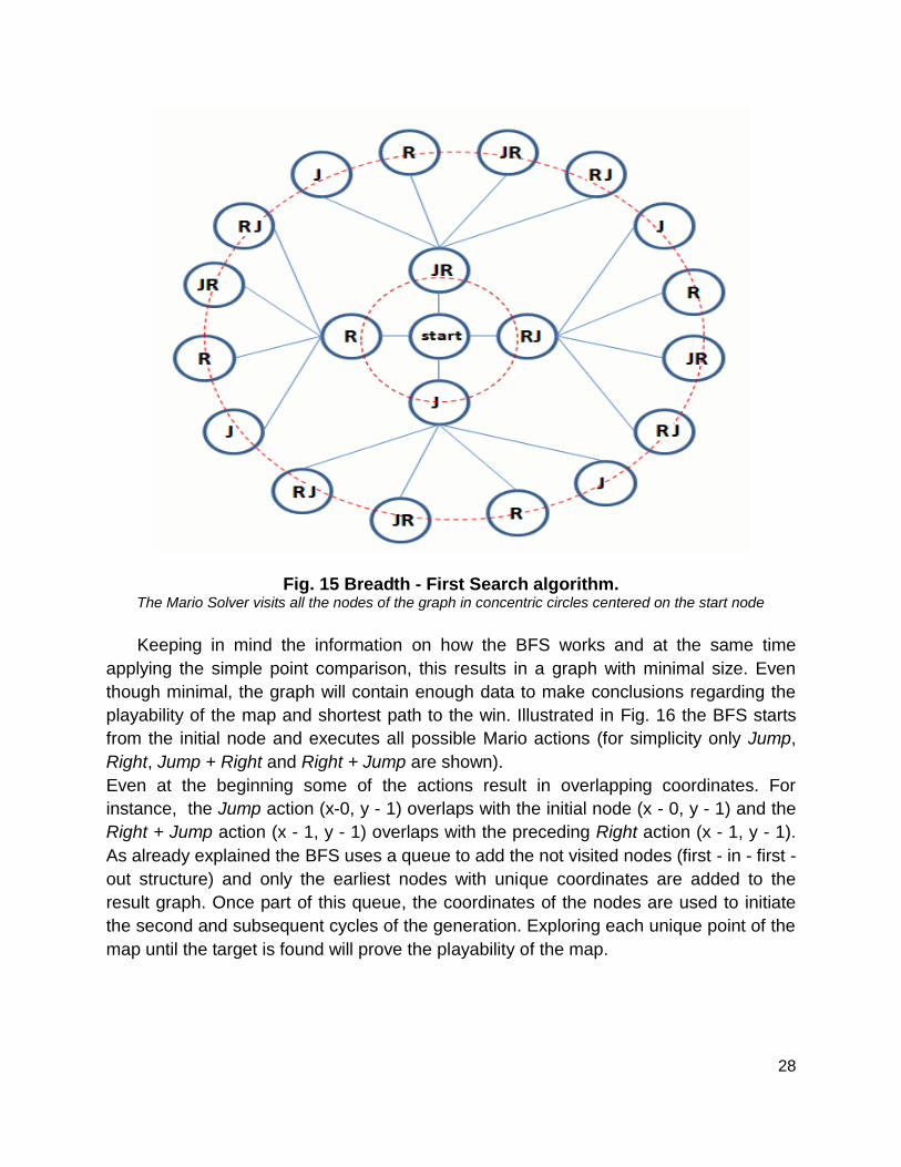
Figure 15 shows how the BFS algorithm is implemented and how the Formula

Generator visits the nodes of the graph in concentric circles, centered on the start node

(action). First, the algorithm starts from the initial Mario node and examines the

immediate neighbors (one edge away) from the action (the inner circle). The examined

nodes are put in a queue - which keeps track of the not visited nodes - and then taking

them from the same queue based on their input order (first - in - first - out) the second

circle is constructed. Repeating the same process again and again, the algorithm

continues until the target vertex is found. The work of the algorithm defines one of its

most important properties – it is capable of finding the shortest path. If the length of the

path is defined as the number of constituted edges or nodes contained in the graph,

then when the algorithm is applied to the graph of Mario actions starting from any

vertex, the resulting search graph gives shortest paths from the initial node to every

other vertex in the graph.

28

Fig. 15 Breadth - First Search algorithm. The Mario Solver visits all the nodes of the graph in concentric circles centered on the start node

Keeping in mind the information on how the BFS works and at the same time

applying the simple point comparison, this results in a graph with minimal size. Even

though minimal, the graph will contain enough data to make conclusions regarding the

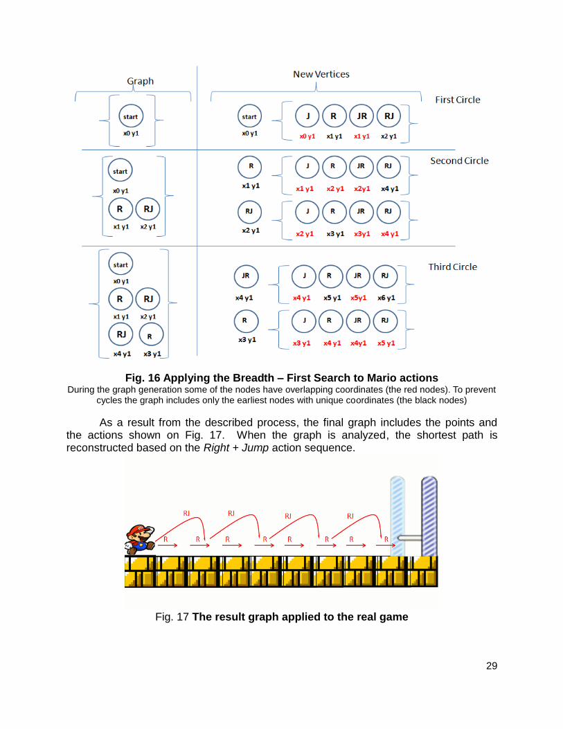
playability of the map and shortest path to the win. Illustrated in Fig. 16 the BFS starts

from the initial node and executes all possible Mario actions (for simplicity only Jump,

Right, Jump + Right and Right + Jump are shown).

Even at the beginning some of the actions result in overlapping coordinates. For

instance, the Jump action (x-0, y - 1) overlaps with the initial node (x - 0, y - 1) and the

Right + Jump action (x - 1, y - 1) overlaps with the preceding Right action (x - 1, y - 1).

As already explained the BFS uses a queue to add the not visited nodes (first - in - first -

out structure) and only the earliest nodes with unique coordinates are added to the

result graph. Once part of this queue, the coordinates of the nodes are used to initiate

the second and subsequent cycles of the generation. Exploring each unique point of the

map until the target is found will prove the playability of the map.

29

Fig. 16 Applying the Breadth – First Search to Mario actions

During the graph generation some of the nodes have overlapping coordinates (the red nodes). To prevent cycles the graph includes only the earliest nodes with unique coordinates (the black nodes)

As a result from the described process, the final graph includes the points and the actions shown on Fig. 17. When the graph is analyzed, the shortest path is reconstructed based on the Right + Jump action sequence.

Fig. 17 The result graph applied to the real game

30

4.3 Algorithm Limitations

The program is somewhat restricted compared to the real game - these

restrictions are chosen to simplify the solution and to fit the timeframe of the project.

The aim is to render probable, that this approach is a viable way to solve the problem -

the verification of PCG artifacts. This being the case, the simplifications has to be

reasonable, so that a found wining-path will be convincing.

The limits here are regarding the chosen search algorithm and not about the

artifacts that are excluded. The latter are covered in 5.3 Expanding the solution.

Since the algorithm is a BFS it inherits the same general limitations. For instance,

if the map length is increased, this is not a problem. However, if the solver covers more

action combinations (see - 5.3.3 Extending the number of Mario actions) the impact could

be severe.

In the current solution we operate with 3 basic actions and 4 combinations of

actions. To map the real game we have to operate with many times more combinations.

As a consequence of that, the algorithm will have a lot more child-nodes to visit, and

thereby increasing the graph considerably.

As the name suggest the Breath-first-search (BFS) is well suited to a wide

solution - even if we prolong the map several times, the BFS will do the job fine, but if

the graph is deepened (like the aforementioned increase of actions) , another search

algorithm could be necessary or at least better suited.

The program does find the winning path. The current solution finds the shortest in

regards to steps travelled. However, if the goal is not the steps travelled an algorithm

like Dijkstra would be better suited (see further details in Different search algorithm).

4.4 Performance

As previously stated the current project is based on flexible experimental design

and it allows quantitative measurements on specific variables. The performance of the

solution is seen as such. The measurements are out of the main project scope, but they

are used as a guideline for refining the solution. Even though, the code base was

subject to constant change and these measurements were not noted down continuously

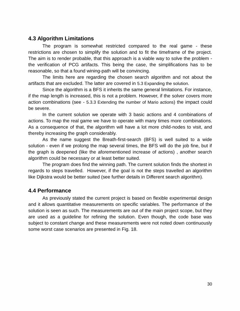
some worst case scenarios are presented in Fig. 18.

31

Fig. 18 The Mario Solver performance

The presented results show the Mario Solver performance in case of the biggest map tried.

The PCG map is produced by the in - game level generator and features linear level design. The results

are acquired from Windows XP, VirtualBox4.1.4, Intel i7 8MB L2, 8Gb

An additional reason for presenting the results is due to the idea that the solution

could be adapted, so it could be used during runtime. For instance, when the game

generates a map, the solver could verify that it is playable. To do this it is necessary to

know which kind of performance we're talking about. Since it is only a thought, this is

not pursued further in the report.

32

5. Discussion

This section of the report discusses some core decisions, options and changes,

one could try to expand and/or improve the current solution. The overall goal of the

improvements is to get closer to the real game and provide new knowledge.

5.1 The Granularity of the logic

As stated throughout the report, the current solution is simplified and operates on

crude assumptions, making the logic coarse. The simplifications include not only the

limited number of game elements (Fig. 3), but also the movement details. To illustrate

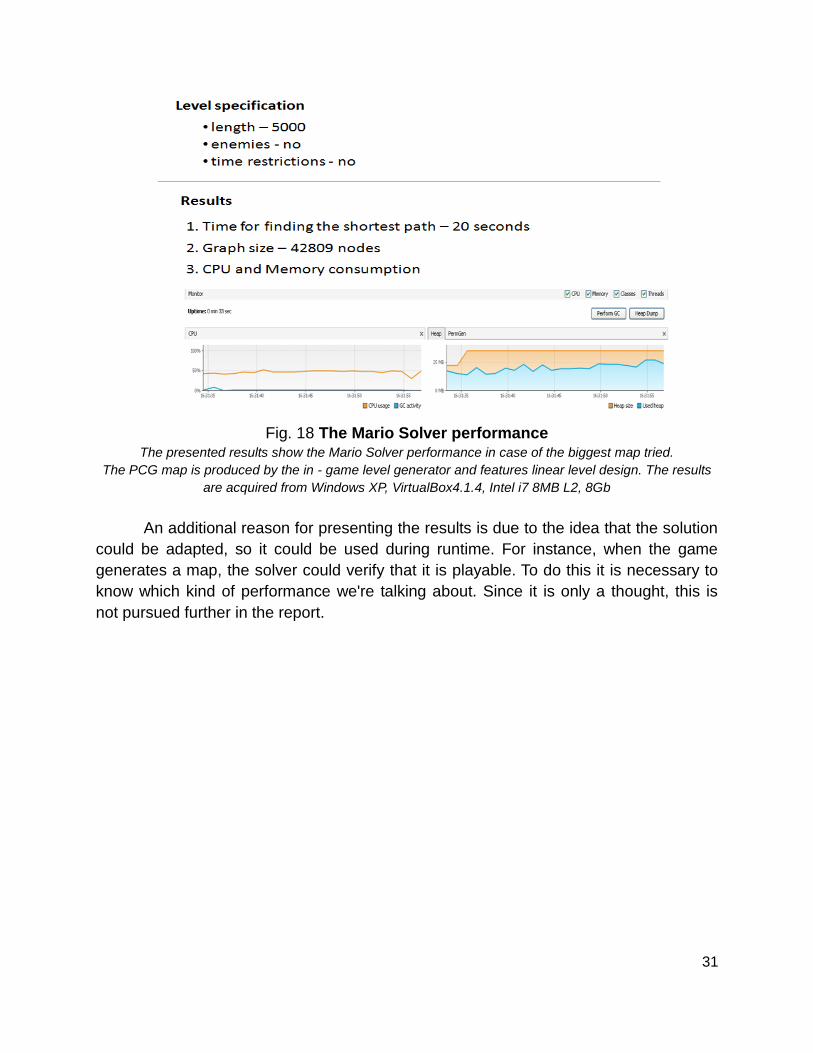
the idea behind the movement simplifications Fig. 19 is presented. In the Mario Solver

one Right action brings Mario one block ahead. In contrast, the real game achieves the

same result by performing sixteen distinct Right actions and game ticks. At first such a

simplification looks like it oversimplifies the behavior of the real game, but when it is put

in the perspective of the playability of the maps, no significant details found are

excluded.

Fig 19 Movement simplifications.

The Mario Solver operates on a super step size (one action brings Mario at least one block forwards or backwards). However, in the real game to accomplish the same result, sixteen

individual actions are needed.

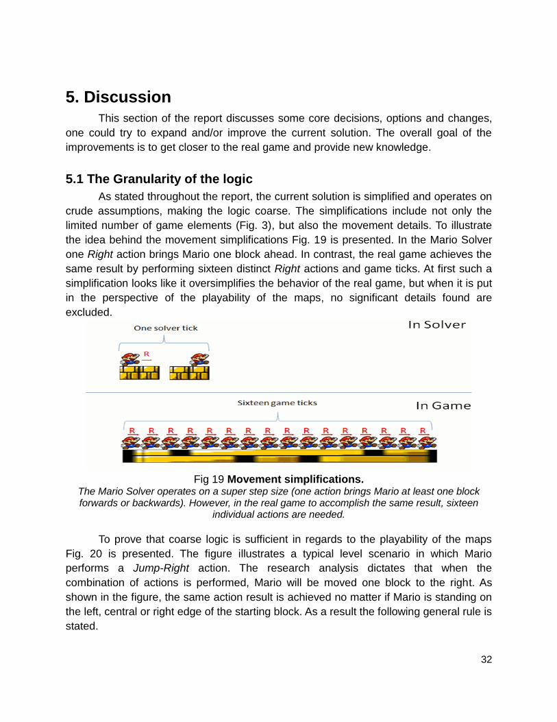
To prove that coarse logic is sufficient in regards to the playability of the maps

Fig. 20 is presented. The figure illustrates a typical level scenario in which Mario

performs a Jump-Right action. The research analysis dictates that when the

combination of actions is performed, Mario will be moved one block to the right. As

shown in the figure, the same action result is achieved no matter if Mario is standing on

the left, central or right edge of the starting block. As a result the following general rule is

stated.

33

As long as Mario stays within the same map unit (block or air) and the game

components correspond to the elements on Fig. 3, his state will be constant

across the unit.

Fig. 20 Reason for making super steps No matter if Mario jumps from the left, central or right edge of a block the result state of Mario

will be ↑ (lives). The same result will be produced from any of the block points.

Based on this assumption, we find that all equivalent steps from a map unit can

be collapsed into one, resulting into smaller graph and less computations.

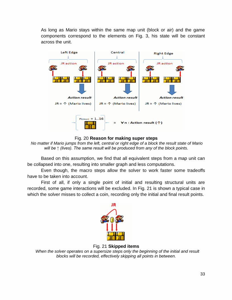
Even though, the macro steps allow the solver to work faster some tradeoffs

have to be taken into account.

First of all, if only a single point of initial and resulting structural units are

recorded, some game interactions will be excluded. In Fig. 21 is shown a typical case in

which the solver misses to collect a coin, recording only the initial and final result points.

Fig. 21 Skipped items

When the solver operates on a supersize steps only the beginning of the initial and result blocks will be recorded, effectively skipping all points in between.

34

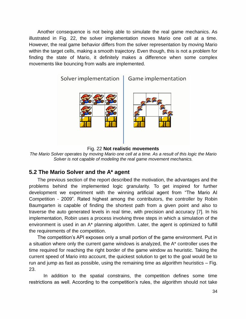
Another consequence is not being able to simulate the real game mechanics. As

illustrated in Fig. 22, the solver implementation moves Mario one cell at a time.

However, the real game behavior differs from the solver representation by moving Mario

within the target cells, making a smooth trajectory. Even though, this is not a problem for

finding the state of Mario, it definitely makes a difference when some complex

movements like bouncing from walls are implemented.

Fig. 22 Not realistic movements

The Mario Solver operates by moving Mario one cell at a time. As a result of this logic the Mario Solver is not capable of modeling the real game movement mechanics.

5.2 The Mario Solver and the A* agent

The previous section of the report described the motivation, the advantages and the

problems behind the implemented logic granularity. To get inspired for further

development we experiment with the winning artificial agent from “The Mario AI

Competition - 2009”. Rated highest among the contributors, the controller by Robin

Baumgarten is capable of finding the shortest path from a given point and also to

traverse the auto generated levels in real time, with precision and accuracy [7]. In his

implementation, Robin uses a process involving three steps in which a simulation of the

environment is used in an A* planning algorithm. Later, the agent is optimized to fulfill

the requirements of the competition.

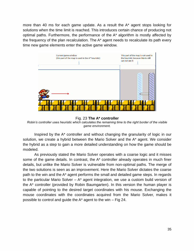
The competition’s API exposes only a small portion of the game environment. Put in

a situation where only the current game windows is analyzed, the A* controller uses the

time required for reaching the right border of the game window as heuristic. Taking the

current speed of Mario into account, the quickest solution to get to the goal would be to

run and jump as fast as possible, using the remaining time as algorithm heuristics – Fig.

23.

In addition to the spatial constrains, the competition defines some time

restrictions as well. According to the competition’s rules, the algorithm should not take

35

more than 40 ms for each game update. As a result the A* agent stops looking for

solutions when the time limit is reached. This introduces certain chance of producing not

optimal paths. Furthermore, the performance of the A* algorithm is mostly affected by

the frequency of the plan recalculation. The A* agent needs to recalculate its path every

time new game elements enter the active game window.

Fig. 23 The A* controller Robin’s controller uses heuristic which calculates the remaining time to the right border of the visible

game environment.

Inspired by the A* controller and without changing the granularity of logic in our

solution, we create a hybrid between the Mario Solver and the A* agent. We consider

the hybrid as a step to gain a more detailed understanding on how the game should be

modeled.

As previously stated the Mario Solver operates with a coarse logic and it misses

some of the game details. In contrast, the A* controller already operates in much finer

details, but unlike the Mario Solver is vulnerable from non-optimal paths. The merge of

the two solutions is seen as an improvement. Here the Mario Solver dictates the coarse

path to the win and the A* agent performs the small and detailed game steps. In regards

to the particular Mario Solver – A* agent integration, we use a custom build version of

the A* controller (provided by Robin Baumgarten). In this version the human player is

capable of pointing to the desired target coordinates with his mouse. Exchanging the

mouse coordinates with the coordinates acquired from the Mario Solver, makes it

possible to control and guide the A* agent to the win – Fig 24.

36

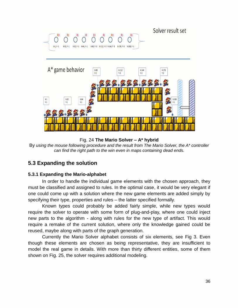
Fig. 24 The Mario Solver – A* hybrid By using the mouse following procedure and the result from The Mario Solver, the A* controller

can find the right path to the win even in maps containing dead ends.

5.3 Expanding the solution

5.3.1 Expanding the Mario-alphabet

In order to handle the individual game elements with the chosen approach, they

must be classified and assigned to rules. In the optimal case, it would be very elegant if

one could come up with a solution where the new game elements are added simply by

specifying their type, properties and rules – the latter specified formally.

Known types could probably be added fairly simple, while new types would

require the solver to operate with some form of plug-and-play, where one could inject

new parts to the algorithm - along with rules for the new type of artifact. This would

require a remake of the current solution, where only the knowledge gained could be

reused, maybe along with parts of the graph generation.

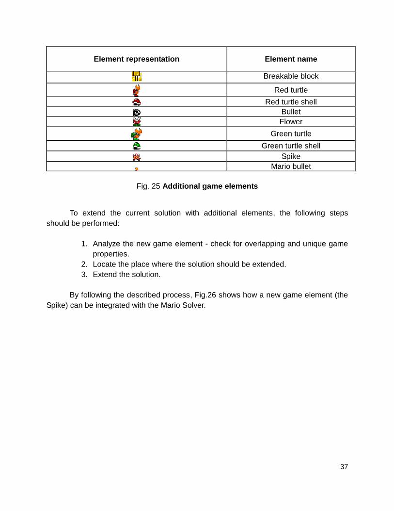
Currently the Mario Solver alphabet consists of six elements, see Fig 3. Even

though these elements are chosen as being representative, they are insufficient to

model the real game in details. With more than thirty different entities, some of them

shown on Fig. 25, the solver requires additional modeling.

37

Element representation Element name

Breakable block

Red turtle

Red turtle shell

Bullet

Flower

Green turtle

Green turtle shell

Spike

Mario bullet

Fig. 25 Additional game elements

To extend the current solution with additional elements, the following steps

should be performed:

1. Analyze the new game element - check for overlapping and unique game

properties.

2. Locate the place where the solution should be extended.

3. Extend the solution.

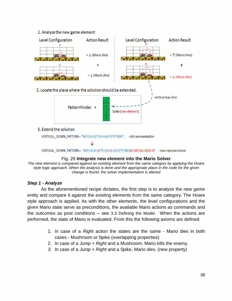
By following the described process, Fig.26 shows how a new game element (the

Spike) can be integrated with the Mario Solver.

38

Fig. 26 Integrate new element into the Mario Solver

The new element is compared against an existing element from the same category by applying the Hoare style logic approach. When the analysis is done and the appropriate place in the code for the given

change is found, the solver implementation is altered

Step 1 - Analyze

As the aforementioned recipe dictates, the first step is to analyze the new game

entity and compare it against the existing elements from the same category. The Hoare

style approach is applied. As with the other elements, the level configurations and the

given Mario state serve as preconditions, the available Mario actions as commands and

the outcomes as post conditions – see 3.3 Defining the Model. When the actions are

performed, the state of Mario is evaluated. From this the following axioms are defined.

1. In case of a Right action the states are the same - Mario dies in both

cases - Mushroom or Spike (overlapping properties)

2. In case of a Jump + Right and a Mushroom, Mario kills the enemy.

3. In case of a Jump + Right and a Spike, Mario dies. (new property)

39

Step 2 - Locate the place for extension.

By analyzing the solver the most appropriate place for the change is selected. As

with other game rules the new property of the Spike is expressed as an axiom - more

specifically a survivability axiom. The Pattern Finder component is responsible for

applying the existing survivability axioms and is therefore the natural choice for the

change.

Step 3 - Extend the solution

Once the right place for the change is found, the last step is to alter the existing

implementation. In this case the regular expressions regarding the vertical matching are

altered. The new expression includes information for handling the new element.

The process above shows how to incorporate new enemy elements into the

existing solution. This procedure is flexible enough to accommodate not only enemies,

but also various structural and nonstructural elements. For instance, when modeling

breakable blocks they are the same as the ordinary blocks, except when they are hit by

Mario from underneath - they break and disappear. This behavior could easily be

applied by following the describe process.

5.3.2 Extending the game characteristics and the step size

The current version of the solver operates in super steps (see 5.1 The Granularity

of the logic). The main reason for doing so is that the coarse logic keeps the result graph

small and it is still expressive enough to model the real game. To add further value to

the research, there is a need to bring the current solver implementation closer to the

real game. For instance, one of the important game factors, which is absent from the

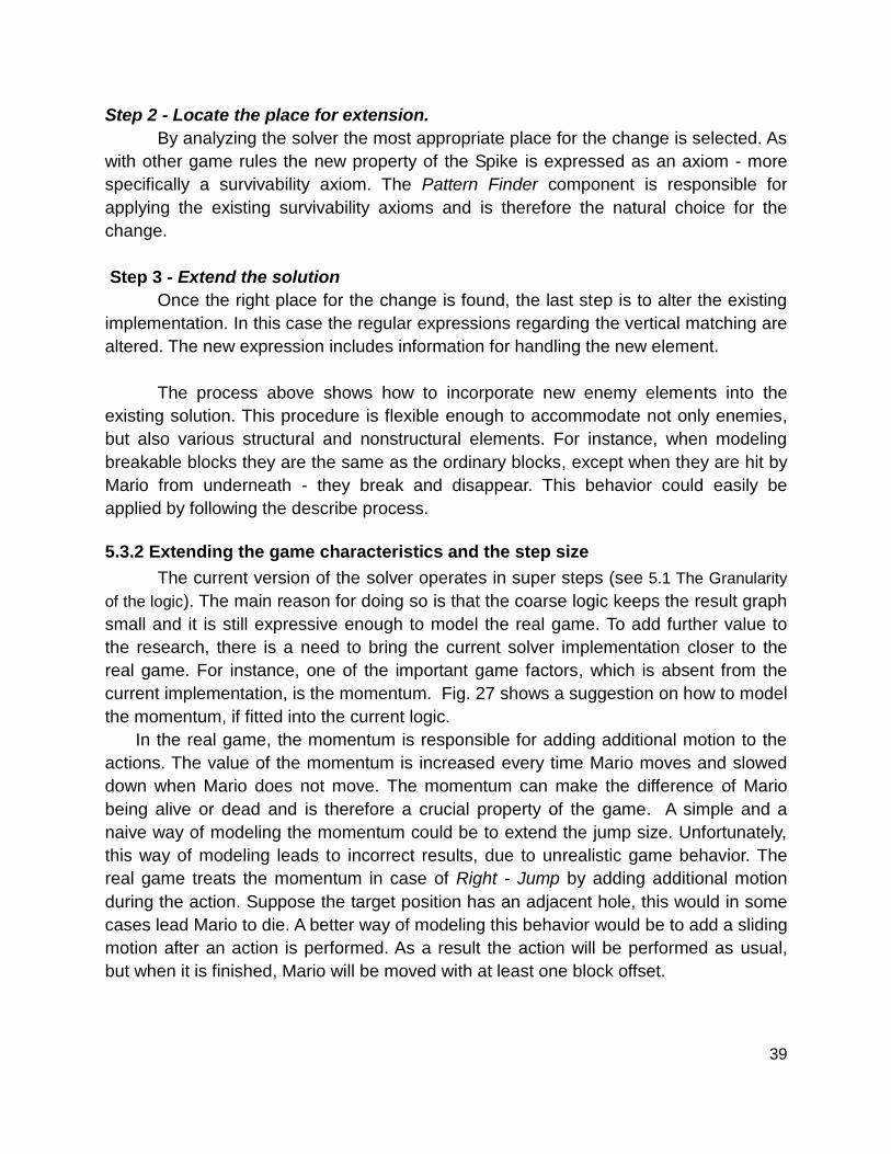
current implementation, is the momentum. Fig. 27 shows a suggestion on how to model

the momentum, if fitted into the current logic.

In the real game, the momentum is responsible for adding additional motion to the

actions. The value of the momentum is increased every time Mario moves and slowed

down when Mario does not move. The momentum can make the difference of Mario

being alive or dead and is therefore a crucial property of the game. A simple and a

naive way of modeling the momentum could be to extend the jump size. Unfortunately,

this way of modeling leads to incorrect results, due to unrealistic game behavior. The

real game treats the momentum in case of Right - Jump by adding additional motion

during the action. Suppose the target position has an adjacent hole, this would in some

cases lead Mario to die. A better way of modeling this behavior would be to add a sliding

motion after an action is performed. As a result the action will be performed as usual,

but when it is finished, Mario will be moved with at least one block offset.

40

Fig. 27 Adding momentum to the current solution

An investigation on how the momentum will fit into the simplified logic. Two solutions are considered – to

increase the jump size or to add sliding.

As just shown the momentum can be modeled by the current version of the

solver. However, due to the game simplifications and the granularity level of the logic,

the least amount of momentum is one block. Operating on a much finer scale, the real

game (remember one block element contains sixteen different possible coordinates)

allows richer details in terms of rules and entity interactions.

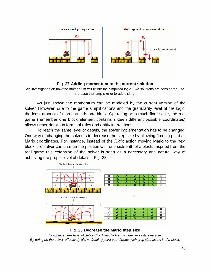
To reach the same level of details, the solver implementation has to be changed.

One way of changing the solver is to decrease the step size by allowing floating point as

Mario coordinates. For instance, instead of the Right action moving Mario to the next

block, the solver can change the position with one sixteenth of a block. Inspired from the

real game this extension of the solver is seen as a necessary and natural way of

achieving the proper level of details – Fig. 28.

Fig. 28 Decrease the Mario step size

To achieve finer level of details the Mario Solver can decrease its step size.

By doing so the solver effectively allows floating point coordinates with step size as 1/16 of a block.

41

Even though the proposed step size brings the solver implementation much

closer to the real game, dealing with floating point values can be difficult.

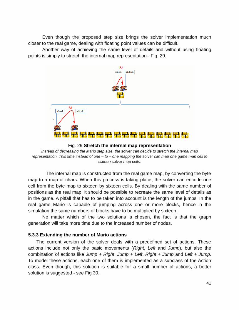
Another way of achieving the same level of details and without using floating

points is simply to stretch the internal map representation– Fig. 29.

Fig. 29 Stretch the internal map representation

Instead of decreasing the Mario step size, the solver can decide to stretch the internal map

representation. This time instead of one – to – one mapping the solver can map one game map cell to

sixteen solver map cells.

The internal map is constructed from the real game map, by converting the byte

map to a map of chars. When this process is taking place, the solver can encode one

cell from the byte map to sixteen by sixteen cells. By dealing with the same number of

positions as the real map, it should be possible to recreate the same level of details as

in the game. A pitfall that has to be taken into account is the length of the jumps. In the

real game Mario is capable of jumping across one or more blocks, hence in the

simulation the same numbers of blocks have to be multiplied by sixteen.

No matter which of the two solutions is chosen, the fact is that the graph

generation will take more time due to the increased number of nodes.

5.3.3 Extending the number of Mario actions

The current version of the solver deals with a predefined set of actions. These

actions include not only the basic movements (Right, Left and Jump), but also the

combination of actions like Jump + Right, Jump + Left, Right + Jump and Left + Jump.

To model these actions, each one of them is implemented as a subclass of the Action

class. Even though, this solution is suitable for a small number of actions, a better

solution is suggested - see Fig 30.

42

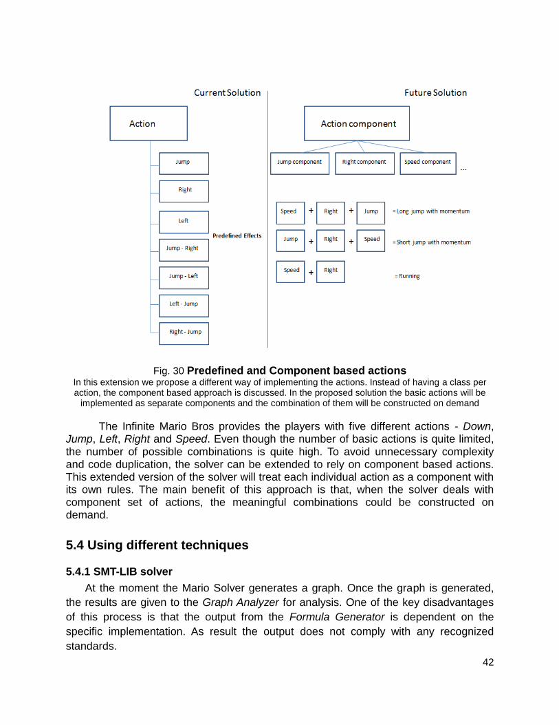
Fig. 30 Predefined and Component based actions

In this extension we propose a different way of implementing the actions. Instead of having a class per action, the component based approach is discussed. In the proposed solution the basic actions will be

implemented as separate components and the combination of them will be constructed on demand

The Infinite Mario Bros provides the players with five different actions - Down, Jump, Left, Right and Speed. Even though the number of basic actions is quite limited, the number of possible combinations is quite high. To avoid unnecessary complexity and code duplication, the solver can be extended to rely on component based actions. This extended version of the solver will treat each individual action as a component with its own rules. The main benefit of this approach is that, when the solver deals with component set of actions, the meaningful combinations could be constructed on demand.

5.4 Using different techniques

5.4.1 SMT-LIB solver

At the moment the Mario Solver generates a graph. Once the graph is generated,

the results are given to the Graph Analyzer for analysis. One of the key disadvantages

of this process is that the output from the Formula Generator is dependent on the

specific implementation. As result the output does not comply with any recognized

standards.

43

As already mentioned the current solution is inspired by PCC and the formal

verification techniques. Instead of creating a proprietary output, one could modify the

solution in a way so it would produce a formula in a standardized format such as SMT-

lib. This output could be interpreted by the already available automated deduction

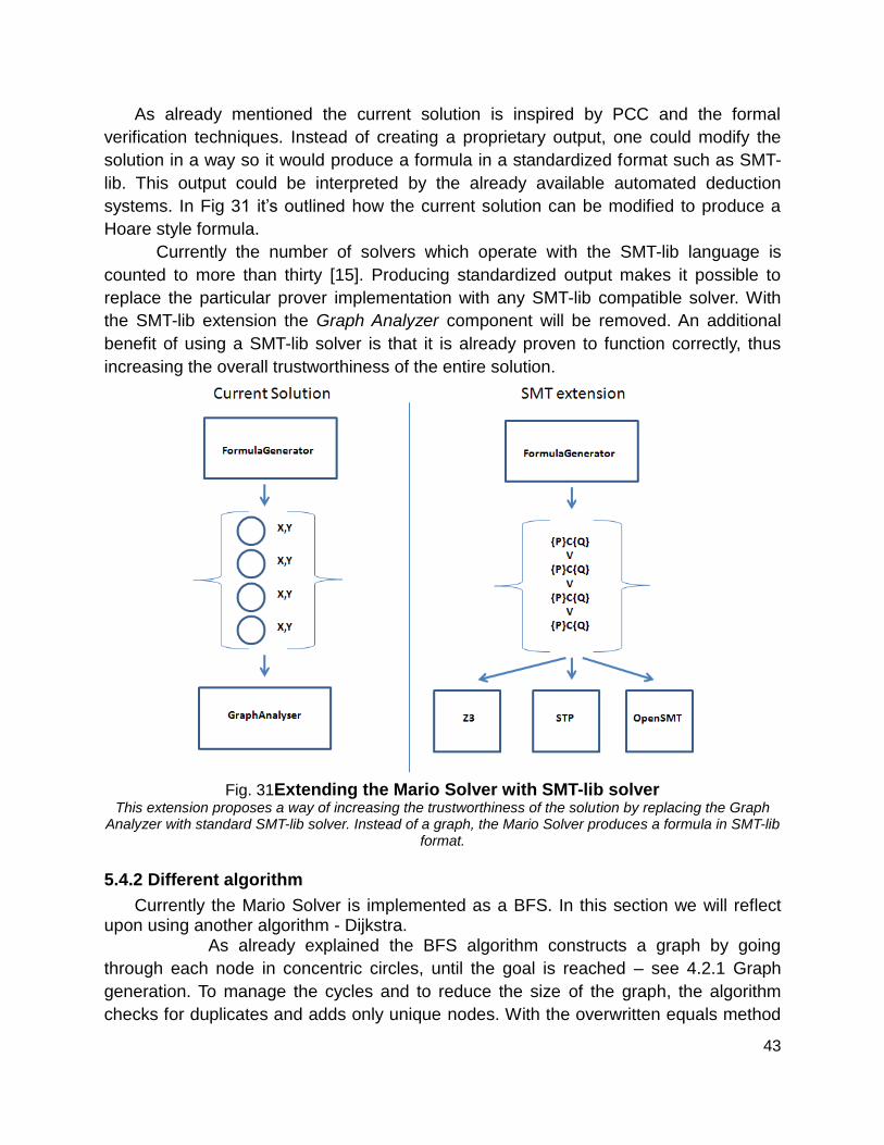
systems. In Fig 31 it’s outlined how the current solution can be modified to produce a

Hoare style formula.

Currently the number of solvers which operate with the SMT-lib language is

counted to more than thirty [15]. Producing standardized output makes it possible to

replace the particular prover implementation with any SMT-lib compatible solver. With

the SMT-lib extension the Graph Analyzer component will be removed. An additional

benefit of using a SMT-lib solver is that it is already proven to function correctly, thus

increasing the overall trustworthiness of the entire solution.

Fig. 31Extending the Mario Solver with SMT-lib solver

This extension proposes a way of increasing the trustworthiness of the solution by replacing the Graph Analyzer with standard SMT-lib solver. Instead of a graph, the Mario Solver produces a formula in SMT-lib

format.

5.4.2 Different algorithm

Currently the Mario Solver is implemented as a BFS. In this section we will reflect upon using another algorithm - Dijkstra.

As already explained the BFS algorithm constructs a graph by going

through each node in concentric circles, until the goal is reached – see 4.2.1 Graph

generation. To manage the cycles and to reduce the size of the graph, the algorithm

checks for duplicates and adds only unique nodes. With the overwritten equals method

44

on the nodes (each node applies the Simple comparison strategy – Fig. 14) only

vertices with unique coordinates, are allowed to enter. When all possibilities are

explored or the target node is found, the algorithm stops and it delivers the result to the

Graph Analyzer – see 4.2.3 Graph-depth - how deep can you go.

In the current solution the output from the model contains unique nodes not part

of the shortest path. This is not a problem since the Graph Analyzer discards these

nodes. If the Graph Analyzer is replaced with a SMT-lib solver the additional nodes will

become a problem. The SMT-lib solvers deal with formal proofs and we don’t see how

they can distinguish between nodes (as triplets) within and outside of the path. To solve

the problem and to remove the additional nodes, the research examines another search

algorithm – the Dijkstra algorithm.

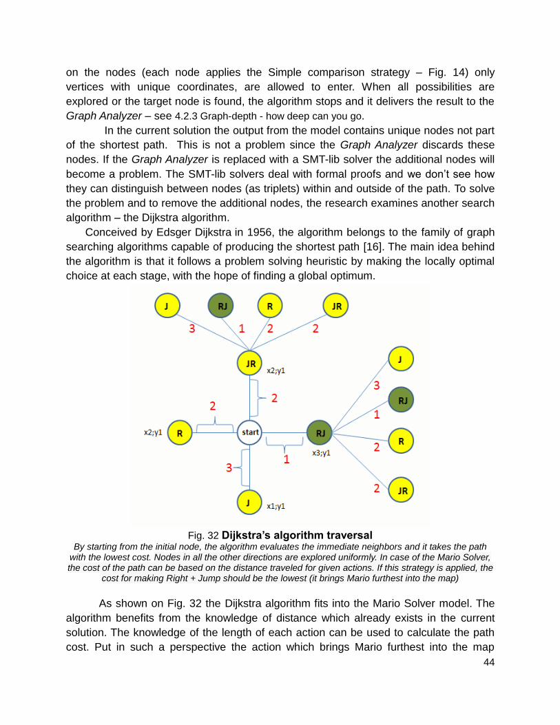
Conceived by Edsger Dijkstra in 1956, the algorithm belongs to the family of graph

searching algorithms capable of producing the shortest path [16]. The main idea behind

the algorithm is that it follows a problem solving heuristic by making the locally optimal

choice at each stage, with the hope of finding a global optimum.

Fig. 32 Dijkstra’s algorithm traversal By starting from the initial node, the algorithm evaluates the immediate neighbors and it takes the path

with the lowest cost. Nodes in all the other directions are explored uniformly. In case of the Mario Solver, the cost of the path can be based on the distance traveled for given actions. If this strategy is applied, the

cost for making Right + Jump should be the lowest (it brings Mario furthest into the map)

As shown on Fig. 32 the Dijkstra algorithm fits into the Mario Solver model. The

algorithm benefits from the knowledge of distance which already exists in the current

solution. The knowledge of the length of each action can be used to calculate the path

cost. Put in such a perspective the action which brings Mario furthest into the map

45

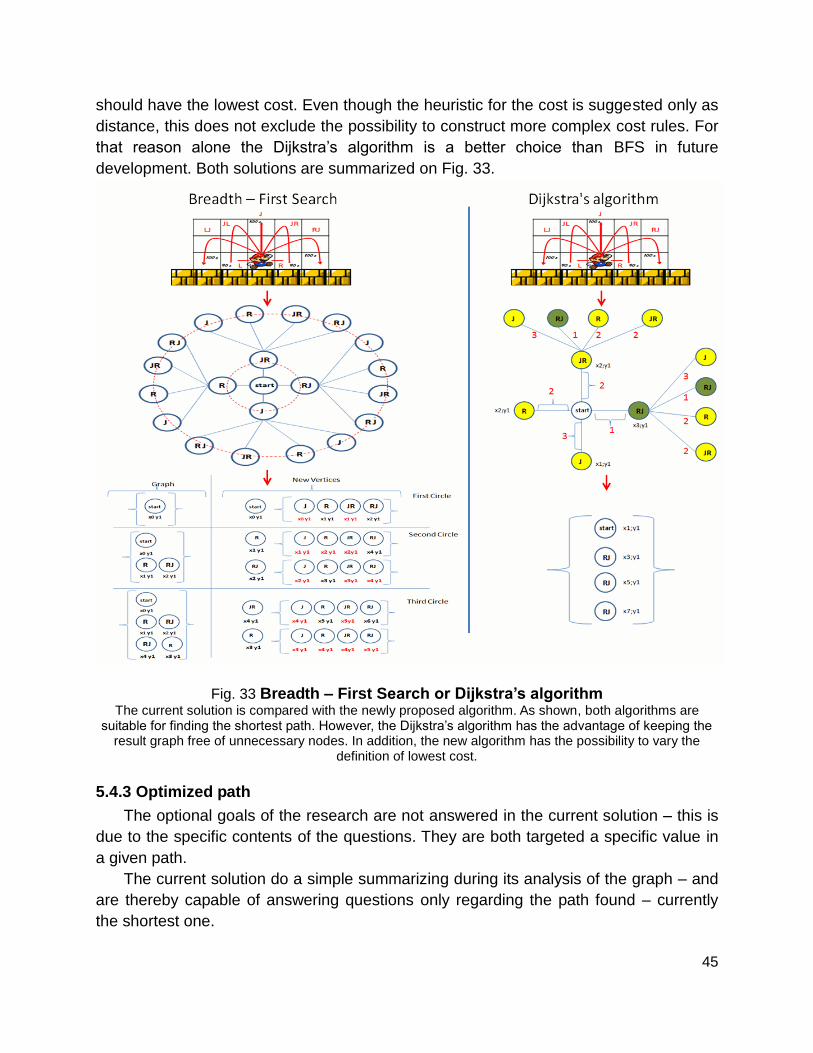
should have the lowest cost. Even though the heuristic for the cost is suggested only as

distance, this does not exclude the possibility to construct more complex cost rules. For

that reason alone the Dijkstra’s algorithm is a better choice than BFS in future

development. Both solutions are summarized on Fig. 33.

Fig. 33 Breadth – First Search or Dijkstra’s algorithm

The current solution is compared with the newly proposed algorithm. As shown, both algorithms are suitable for finding the shortest path. However, the Dijkstra’s algorithm has the advantage of keeping the

result graph free of unnecessary nodes. In addition, the new algorithm has the possibility to vary the definition of lowest cost.

5.4.3 Optimized path

The optional goals of the research are not answered in the current solution – this is

due to the specific contents of the questions. They are both targeted a specific value in

a given path.

The current solution do a simple summarizing during its analysis of the graph – and

are thereby capable of answering questions only regarding the path found – currently

the shortest one.

46

To find answers of this type, the path should be optimized for the specific question.

This can be achieved by a combination of redefining the lowest cost in a Dijkstra’s

search and by changing the goal. The goal has to be defined as a found win, where the

remaining time is zero. This will make the algorithm keep searching even though a win

is found.

If the lowest cost is defined as “most coins to collect”, the path will now be as long

as possible within the given time frame and the edges with most coins will be selected –

thereby being optimized for coins.

It might be to narrow a goal to search for a win, where the remaining time are

exactly zero, but it would be possible to continue searching until the remaining time are

minimal.

6. Conclusion

Even though - as stated throughout the report - the solution operates with a coarse

logic, it is still clear that the derived model is capable of handling the problem of

verifying maps for Infinite Mario Bros.

As shown the PCG maps can be verified with axioms that express the game

behavior. The model based on these axioms - can declare a map valid or invalid.

The secondary goals, which are in regards to the topic of playability, are also

answered. It is possible to find to the shortest path - the path that requires the fewest

steps. Furthermore the solution is capable of finding an answer with a reduced set of

actions - e.g. declaring a given map playable without using the long jump action.

Regarding the optional goals none of them are answered. Both goals require

specific algorithmic behavior, which is not supported by the current solution. Algorithms

which allow different concepts of lowest path cost would be prime candidates to provide

such kind of support. Like suggested, the Dijkstra search algorithm could be

implemented to satisfy these requirements.

47

References

1. A. Doull. “The death of the level designer” Internet: http://pcg.wikidot.com/the-death-of-

the-level-designer, 2008 [May, 29, 2012]

2. A. Couturier and B. Loch, Oral Presentation, Topic, “The procedural generation of indoor

environments for computer games”, Faculty of Mathematics and Informatics, University

of Southern Queensland, 2008

3. N. Shaker, G. N. Yannakakis, and J. Togelius “Towards player-driven procedural content

generation,” in Proceedings of the 9th ACM Computing Frontiers Conference, pp. 237-

240, 2012

4. J. Togelius, S. Karakovskiy, J. Koutnik and J. Schmidhuber “Super Mario Evolution” in

Proceedings of the IEEE Symposium on Computational Intelligence and Games, 2009

5. J. Togelius, G. Yannakakis, K. Stanley, and C. Browne. “Search-based Procedural

Content Generation” A Taxonomy and Survey. Computational Intelligence and AI in

Games, IEEE Transactions on, (99):1 – 1, 2011

6. N. Shaker, J. Togelius, G. Yannakakis, B. Weber, T. Shimizu, T. Hashiyama, N.

Sorenson, P. Pasquier, P. Mawhorter, G. Takahashi, G. Smith, and R. Baumgarten “The

2010 Mario AI Championship: Level Generation Track.”, in IEEE Trans. Comput. Intellig.

and AI in Games; vol. 3, pp. 332-347, 01/2011

7. J. Togelius, S. Karakovskiy and R. Baumgarten “The 2009 Mario AI Competition” in IEEE

Congress on Evolutionary Computation, Proceed-ings. IEEE Press, 2010

8. D. Loiacono, J. Togelius, P. L. Lanzi, L. Kinnaird-Heether, S. M. Lucas, M. Simmerson,

D. Perez, R. G. Reynolds, and Y. Saez, “The WCCI 2008 simulated car racing

competition,” in Proceedings of the IEEE Symposium on Computational Intelligence and

Games, 2008.

9. G. C. Necula. “Proof-carrying code” In Conference Record of POPL '97: The 24th ACM

SIGPLAN-SIGACT Symposium on Principles of Programming Languages, pages 106--

119, Paris, France, 15--17 Jan. 1997.

10. P. Hart, N. Nilsson, and B. Raphael, “A formal basis for the heuristic determination of

minimum cost paths,”IEEE transactions on Systems Science and Cybernetics, vol. 4, no.

2, pp. 100–107, 1968.

48

11. I. Millington and J. Funge. "Artificial Intelligence for Games" Morgan Kaufmann Pub,

2009.

12. T. Mahlmann, A. Drachen, J. Togelius, A. Canossa, and G. N. Yannakakis. "Predicting

Player Behavior in Tomb Raider: Underworld," in Proceedings of the 2010 IEEE

Conference on Computational Intelligence and Games, pp. 178-185

13. C. Pedersen, J. Togelius and G. N. Yannakakis, "Modeling Player Experience for

Content Creation." IEEE Transactions on Computational Intelligence and AI in Games

1(2):121-133, June, 2009.

14. N. Al-Darwish, “Developing and Programming Algorithms”, Jones & Bartlett Learning

2011-03, Section 7.2

15. “SMT-LIB, The Satisfiability Modulo Theories Library, SMT Solvers”: Internet:

http://www.smtlib.org/, [May. 31, 2012]

16. Wikipedia “Dijkstra's algorithm” Internet: http://en.wikipedia.org/wiki/Dijkstra's_algorithm,

May, 23, 2012 [May. 31, 2012]

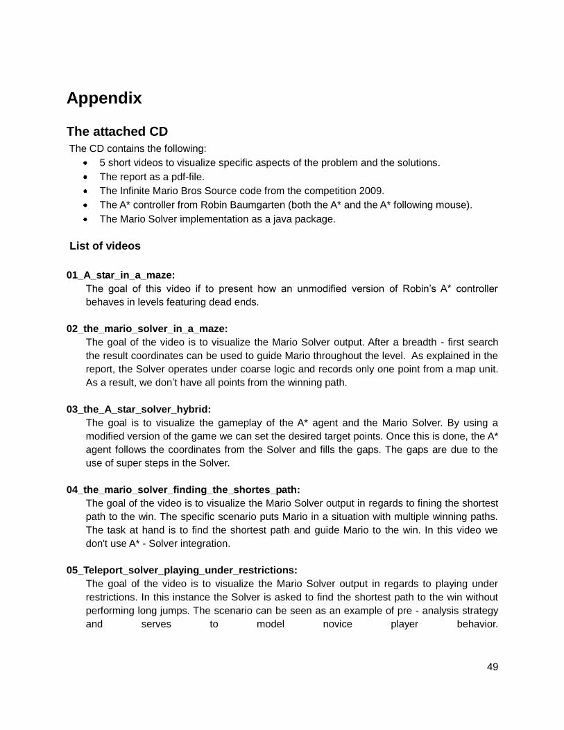
49

Appendix

The attached CD

The CD contains the following:

5 short videos to visualize specific aspects of the problem and the solutions.

The report as a pdf-file.

The Infinite Mario Bros Source code from the competition 2009.

The A* controller from Robin Baumgarten (both the A* and the A* following mouse).

The Mario Solver implementation as a java package.

List of videos

01_A_star_in_a_maze:

The goal of this video if to present how an unmodified version of Robin’s A* controller

behaves in levels featuring dead ends.

02_the_mario_solver_in_a_maze:

The goal of the video is to visualize the Mario Solver output. After a breadth - first search

the result coordinates can be used to guide Mario throughout the level. As explained in the

report, the Solver operates under coarse logic and records only one point from a map unit.

As a result, we don’t have all points from the winning path.

03_the_A_star_solver_hybrid:

The goal is to visualize the gameplay of the A* agent and the Mario Solver. By using a

modified version of the game we can set the desired target points. Once this is done, the A*

agent follows the coordinates from the Solver and fills the gaps. The gaps are due to the

use of super steps in the Solver.

04_the_mario_solver_finding_the_shortes_path:

The goal of the video is to visualize the Mario Solver output in regards to fining the shortest

path to the win. The specific scenario puts Mario in a situation with multiple winning paths.

The task at hand is to find the shortest path and guide Mario to the win. In this video we

don't use A* - Solver integration.

05_Teleport_solver_playing_under_restrictions:

The goal of the video is to visualize the Mario Solver output in regards to playing under

restrictions. In this instance the Solver is asked to find the shortest path to the win without

performing long jumps. The scenario can be seen as an example of pre - analysis strategy

and serves to model novice player behavior.

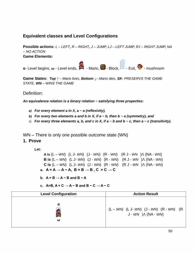
50

Equivalent classes and Level Configurations

Possible actions: L – LEFT, R – RIGHT, J – JUMP, LJ – LEFT JUMP, RJ – RIGHT JUMP, NA

– NO ACTION

Game Elements:

α- Level begins, ω - Level ends, - Mario, - Block, - Exit, - mushroom

Game States: Top ↑ – Mario lives, Bottom ↓– Mario dies, SK- PRESERVS THE GAME

STATE, WN – WINS THE GAME

Definition:

An equivalence relation is a binary relation ~ satisfying three properties:

a) For every element a in X, a ~ a (reflexivity),

b) For every two elements a and b in X, if a ~ b, then b ~ a (symmetry), and

c) For every three elements a, b, and c in X, if a ~ b and b ~ c, then a ~ c (transitivity).

WN – There is only one possible outcome state (WN)

1. Prove

Let:

A is (L – WN)�(L J- WN)�(J - WN)�(R - WN)� (R J - WN�)⋀ (NA - WN)

B is (L – WN)�(L J- WN)�(J - WN)�(R - WN)� (R J - WN�)⋀ (NA - WN)

C is (L – WN)�(L J- WN)�(J - WN)�(R - WN)� (R J - WN�)⋀ (NA - WN)

a. A = A → A ~ A, B = B → B , C = C → C

b. A = B → A ~ B and B ~ A

c. A=B, A = C → A ~ B and B ~ C → A ~ C

Level Configuration Action Result

α

ω

(L – WN)�(L J- WN)�(J - WN)�(R - WN)� (R

J - WN�)⋀ (NA - WN)

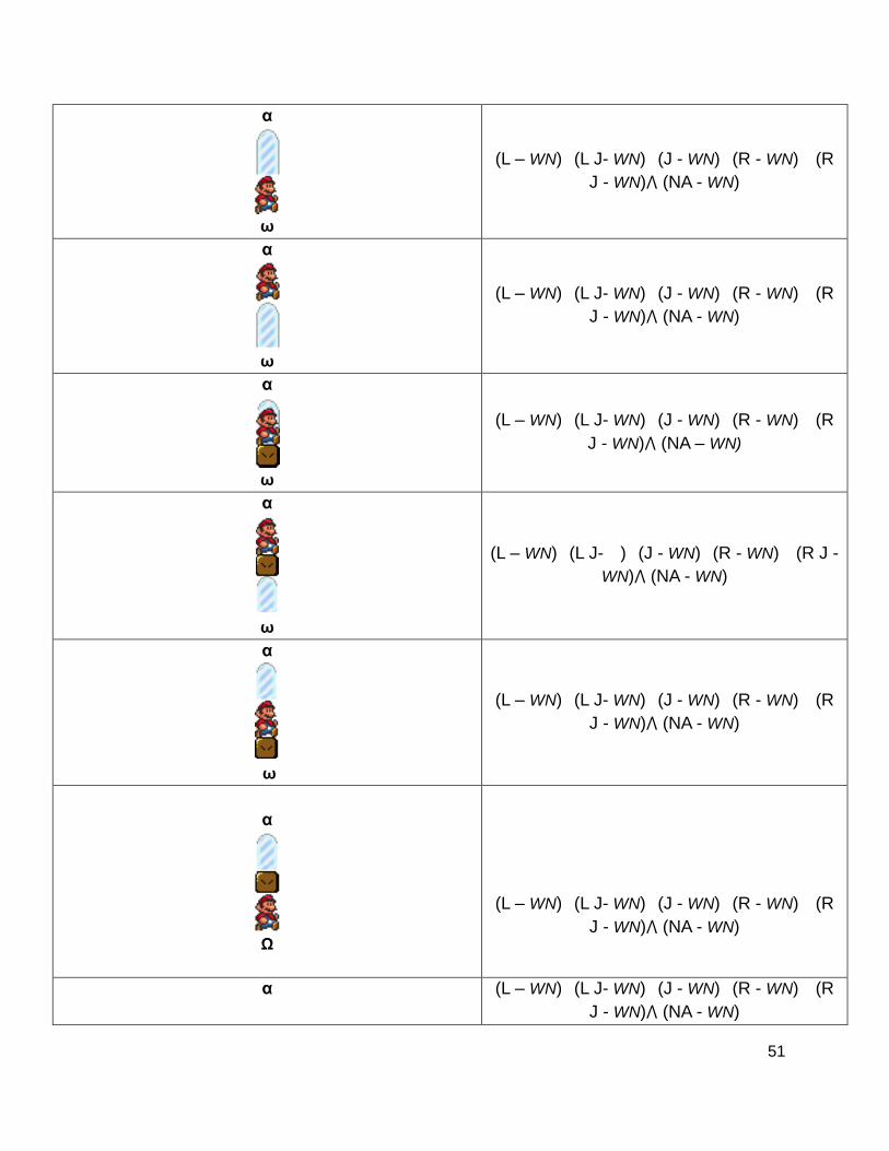
51

α

ω

(L – WN)�(L J- WN)�(J - WN)�(R - WN)� (R

J - WN)⋀ (NA - WN)

α

ω

(L – WN)�(L J- WN)�(J - WN)�(R - WN)� (R

J - WN)⋀ (NA - WN)

α

ω

(L – WN)�(L J- WN)�(J - WN)�(R - WN)� (R

J - WN)⋀ (NA – WN)

α

ω

(L – WN)�(L J- �)�(J - WN)�(R - WN)� (R J -

WN)⋀ (NA - WN)

α

ω

(L – WN)�(L J- WN)�(J - WN)�(R - WN)� (R

J - WN)⋀ (NA - WN)

α

Ω

(L – WN)�(L J- WN)�(J - WN)�(R - WN)� (R

J - WN)⋀ (NA - WN)

α (L – WN)�(L J- WN)�(J - WN)�(R - WN)� (R

J - WN)⋀ (NA - WN)

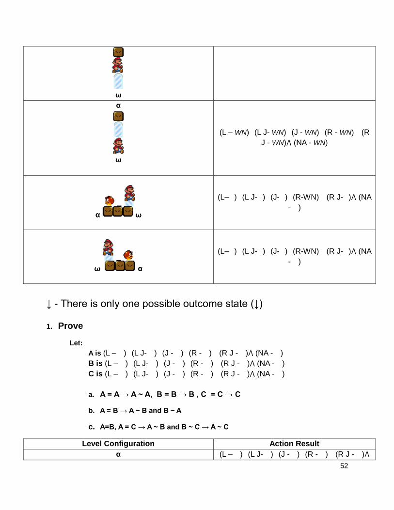
52

ω

α

ω

(L – WN)�(L J- WN)�(J - WN)�(R - WN)� (R

J - WN)⋀ (NA - WN)

α ω

(L–�)�(L J-�)�(J-�)�(R-WN)� (R J-�)⋀ (NA

- �)

ω α

(L–�)�(L J-�)�(J-�)�(R-WN)� (R J-�)⋀ (NA

- �)

↓ - There is only one possible outcome state (↓)

1. Prove

Let:

A is (L – �)�(L J- �)�(J - �)�(R - �)� (R J - �)⋀ (NA - �)

B is (L – �)�(L J- �)�(J - �)�(R - �)� (R J - �)⋀ (NA - �)

C is (L – �)�(L J- �)�(J - �)�(R - �)� (R J - �)⋀ (NA - �)

a. A = A → A ~ A, B = B → B , C = C → C

b. A = B → A ~ B and B ~ A

c. A=B, A = C → A ~ B and B ~ C → A ~ C

Level Configuration Action Result

α (L – �)�(L J- �)�(J - �)�(R - �)� (R J - �)⋀

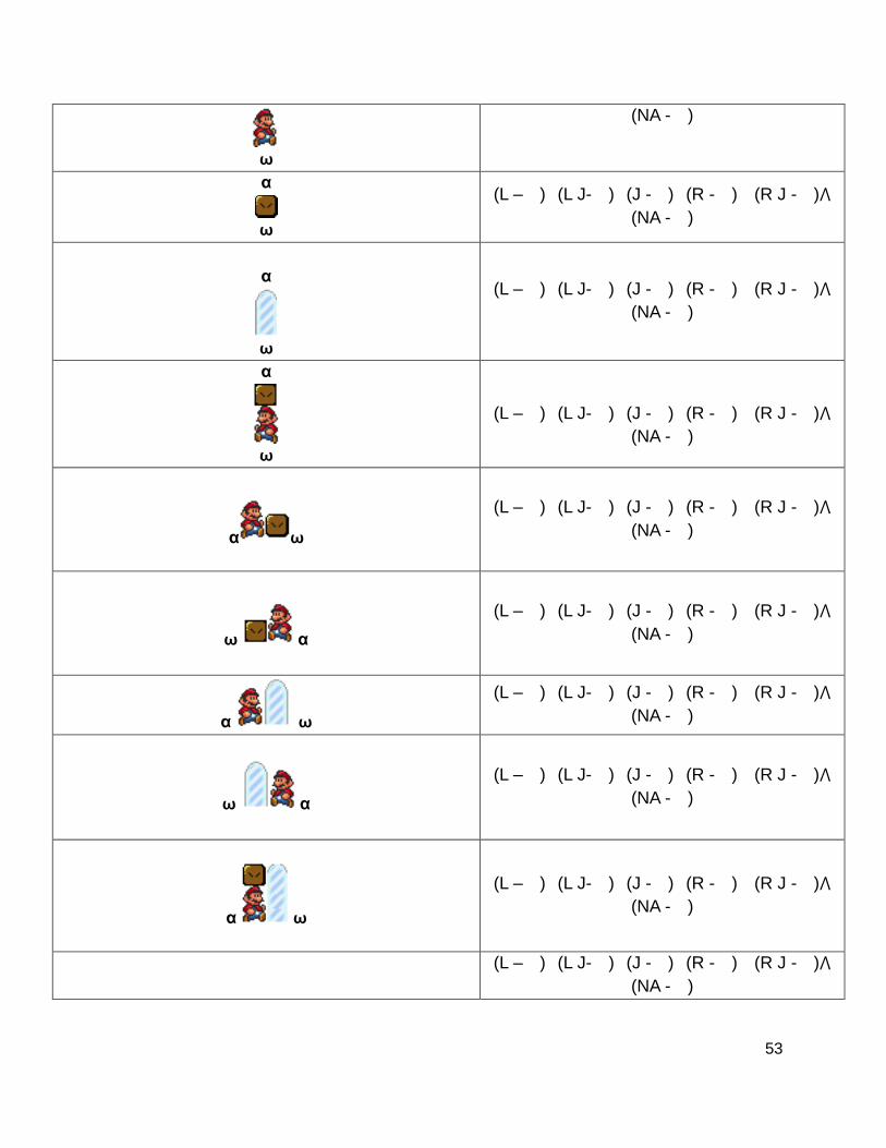
53

ω

(NA - �)

α

ω

(L – �)�(L J- �)�(J - �)�(R - �)� (R J - �)⋀

(NA - �)

α

ω

(L – �)�(L J- �)�(J - �)�(R - �)� (R J - �)⋀

(NA - �)

α

ω

(L – �)�(L J- �)�(J - �)�(R - �)� (R J - �)⋀

(NA - �)

α ω

(L – �)�(L J- �)�(J - �)�(R - �)� (R J - �)⋀

(NA - �)

ω α

(L – �)�(L J- �)�(J - �)�(R - �)� (R J - �)⋀

(NA - �)

α ω

(L – �)�(L J- �)�(J - �)�(R - �)� (R J - �)⋀

(NA - �)

ω α

(L – �)�(L J- �)�(J - �)�(R - �)� (R J - �)⋀

(NA - �)

α ω

(L – �)�(L J- �)�(J - �)�(R - �)� (R J - �)⋀

(NA - �)

(L – �)�(L J- �)�(J - �)�(R - �)� (R J - �)⋀

(NA - �)

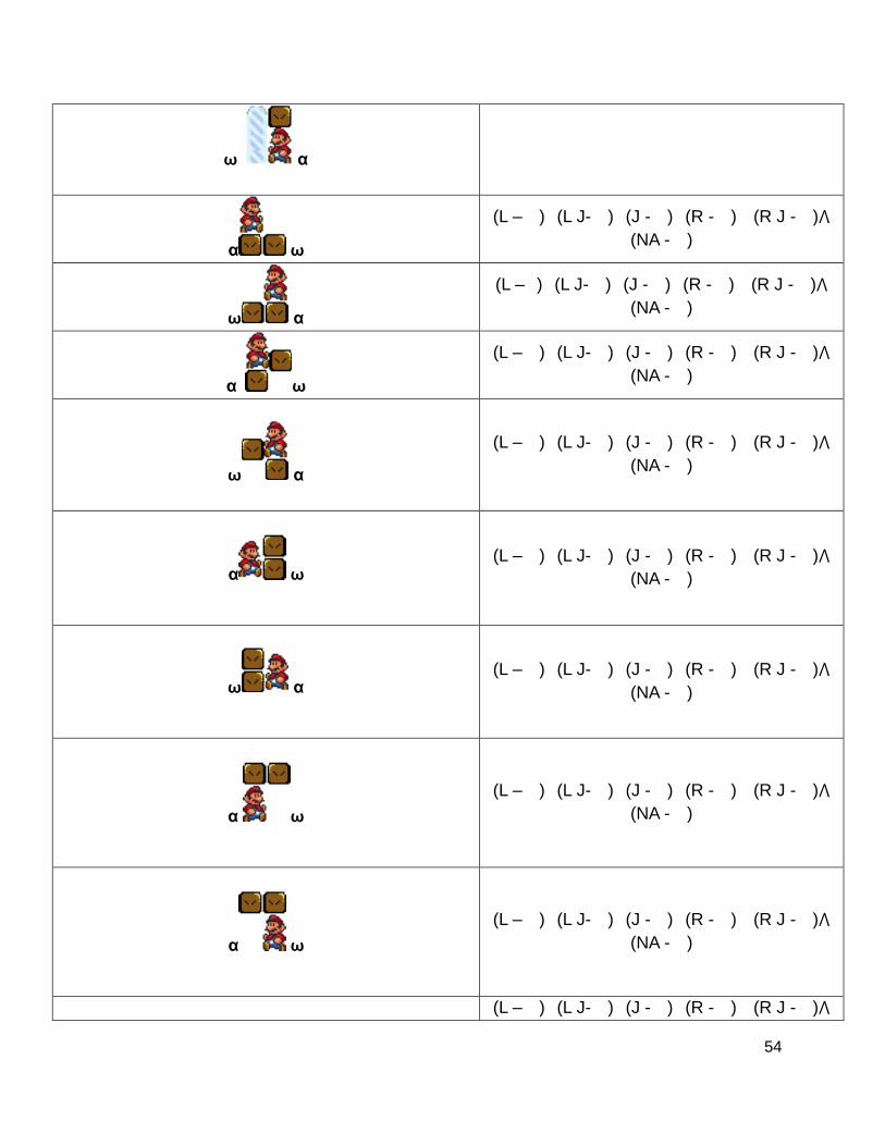
54

ω α

α ω

(L – �)�(L J- �)�(J - �)�(R - �)� (R J - �)⋀

(NA - �)

ω α

(L –�)�(L J- �)�(J - �)�(R - �)� (R J - �)⋀

(NA - �)

α ω

(L – �)�(L J- �)�(J - �)�(R - �)� (R J - �)⋀

(NA - �)

ω α

(L – �)�(L J- �)�(J - �)�(R - �)� (R J - �)⋀

(NA - �)

α ω

(L – �)�(L J- �)�(J - �)�(R - �)� (R J - �)⋀

(NA - �)

ω α

(L – �)�(L J- �)�(J - �)�(R - �)� (R J - �)⋀

(NA - �)

α ω

(L – �)�(L J- �)�(J - �)�(R - �)� (R J - �)⋀

(NA - �)

α ω

(L – �)�(L J- �)�(J - �)�(R - �)� (R J - �)⋀

(NA - �)

(L – �)�(L J- �)�(J - �)�(R - �)� (R J - �)⋀

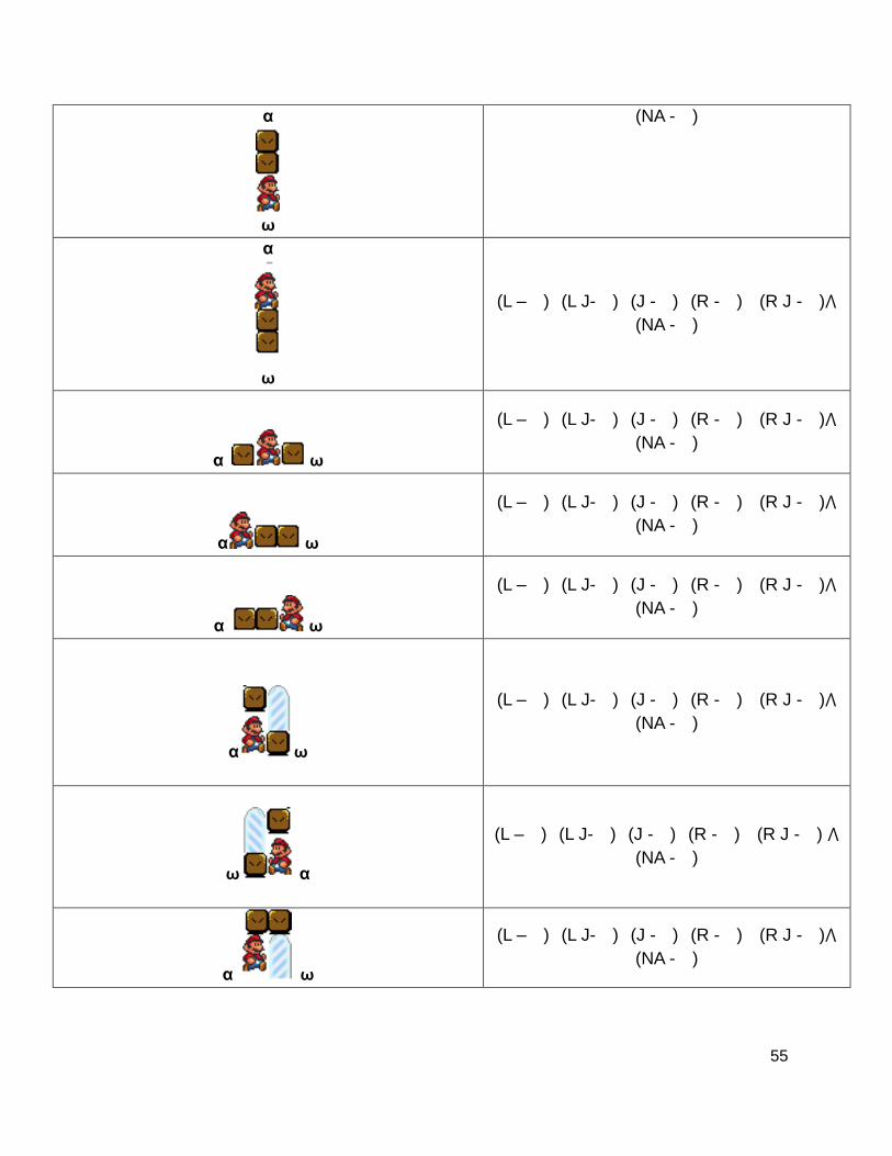
55

α

ω

(NA - �)

α

ω

(L – �)�(L J- �)�(J - �)�(R - �)� (R J - �)⋀

(NA - �)

α ω

(L – �)�(L J- �)�(J - �)�(R - �)� (R J - �)⋀

(NA - �)

α ω

(L – �)�(L J- �)�(J - �)�(R - �)� (R J - �)⋀

(NA - �)

α ω

(L – �)�(L J- �)�(J - �)�(R - �)� (R J - �)⋀

(NA - �)

α ω

(L – �)�(L J- �)�(J - �)�(R - �)� (R J - �)⋀

(NA - �)

ω α

(L – �)�(L J- �)�(J - �)�(R - �)� (R J - �) ⋀

(NA - �)

α ω

(L – �)�(L J- �)�(J - �)�(R - �)� (R J - �)⋀

(NA - �)

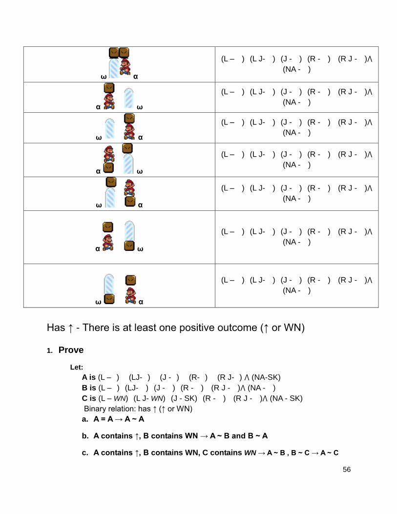
56

ω α

(L – �)�(L J- �)�(J - �)�(R - �)� (R J - �)⋀

(NA - �)

α ω

(L – �)�(L J- �)�(J - �)�(R - �)� (R J - �)⋀

(NA - �)

ω α

(L – �)�(L J- �)�(J - �)�(R - �)� (R J - �)⋀

(NA - �)

α ω

(L – �)�(L J- �)�(J - �)�(R - �)� (R J - �)⋀

(NA - �)

ω α

(L – �)�(L J- �)�(J - �)�(R - �)� (R J - �)⋀

(NA - �)

α ω

(L – �)�(L J- �)�(J - �)�(R - �)� (R J - �)⋀

(NA - �)

ω α

(L – �)�(L J- �)�(J - �)�(R - �)� (R J - �)⋀

(NA - �)

Has ↑ - There is at least one positive outcome (↑ or WN)

1. Prove

Let:

A is (L –�) � (LJ-�) � (J -�) � (R-�) � (R J-�) ⋀ (NA-SK)

B is (L –�)�(LJ- �)�(J - �)�(R - �)� (R J - �)⋀ (NA - �)

C is (L – WN)�(L J- WN)�(J - SK)�(R - �)� (R J - �)⋀ (NA - SK)

Binary relation: has ↑ (↑ or WN)

a. A = A → A ~ A

b. A contains ↑, B contains WN → A ~ B and B ~ A

c. A contains ↑, B contains WN, C contains WN → A ~ B , B ~ C → A ~ C

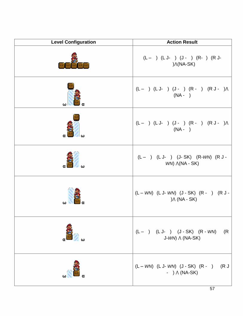
57

Level Configuration Action Result

(L – �)�(L J- �)�(J - �)�(R-�)�(R J-

�)⋀(NA-SK)

ω α

(L – �)�(L J- �)�(J - �)�(R - �)� (R J - �)⋀

(NA - �)

α ω

(L – �)�(L J- �)�(J - �)�(R - �)� (R J - �)⋀

(NA - �)

α ω

(L – �)� (L J- �) �(J- SK)� (R-WN)�(R J -

WN) ⋀(NA - SK)

ω α

(L – WN)�(L J- WN)�(J - SK)�(R - �)� (R J -

�)⋀ (NA - SK)

α ω

(L – �) � (L J- �) � (J - SK)� (R - WN) � (R

J-WN) ⋀ (NA-SK)

ω α

(L – WN)�(L J- WN)�(J - SK)�(R - �) � (R J

- �) ⋀ (NA-SK)

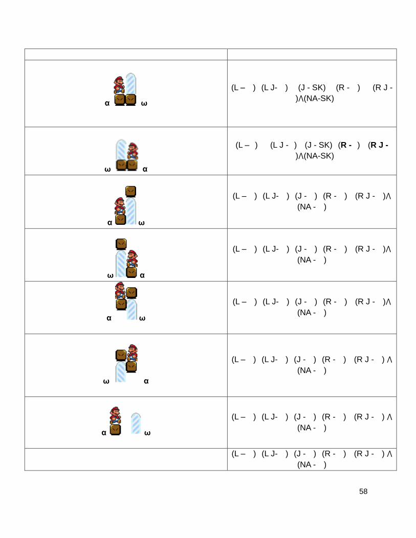
58

α ω

(L – �)�(L J- �) � (J - SK) � (R - �) � (R J -

�)⋀(NA-SK)

ω α

(L –�) � (L J -�) �(J - SK)�(R -�)� (R J -

�)⋀(NA-SK)

α ω

(L – �)�(L J- �)�(J - �)�(R - �)� (R J - �)⋀

(NA - �)

ω α

(L – �)�(L J- �)�(J - �)�(R - �)� (R J - �)⋀

(NA - �)

α ω

(L – �)�(L J- �)�(J - �)�(R - �)� (R J - �)⋀

(NA - �)

ω α

(L – �)�(L J- �)�(J - �)�(R - �)� (R J - �) ⋀

(NA - �)

α ω

(L – �)�(L J- �)�(J - �)�(R - �)� (R J - �) ⋀

(NA - �)

(L – �)�(L J- �)�(J - �)�(R - �)� (R J - �) ⋀

(NA - �)

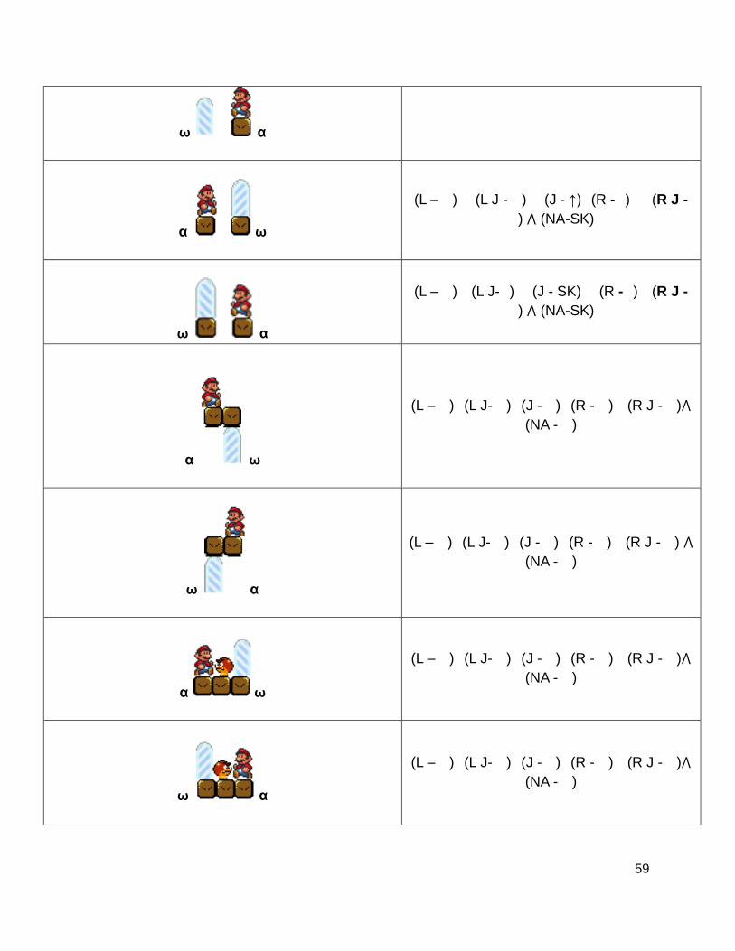
59

ω α

α ω

(L – �) � (L J - �) � (J - ↑)�(R -�) � (R J -

�) ⋀ (NA-SK)

ω α

(L – �)� (L J-�) � (J - SK) � (R -�)� (R J -

�) ⋀ (NA-SK)

α ω

(L – �)�(L J- �)�(J - �)�(R - �)� (R J - �)⋀

(NA - �)

ω α

(L – �)�(L J- �)�(J - �)�(R - �)� (R J - �) ⋀

(NA - �)

α ω

(L – �)�(L J- �)�(J - �)�(R - �)� (R J - �)⋀

(NA - �)

ω α

(L – �)�(L J- �)�(J - �)�(R - �)� (R J - �)⋀

(NA - �)

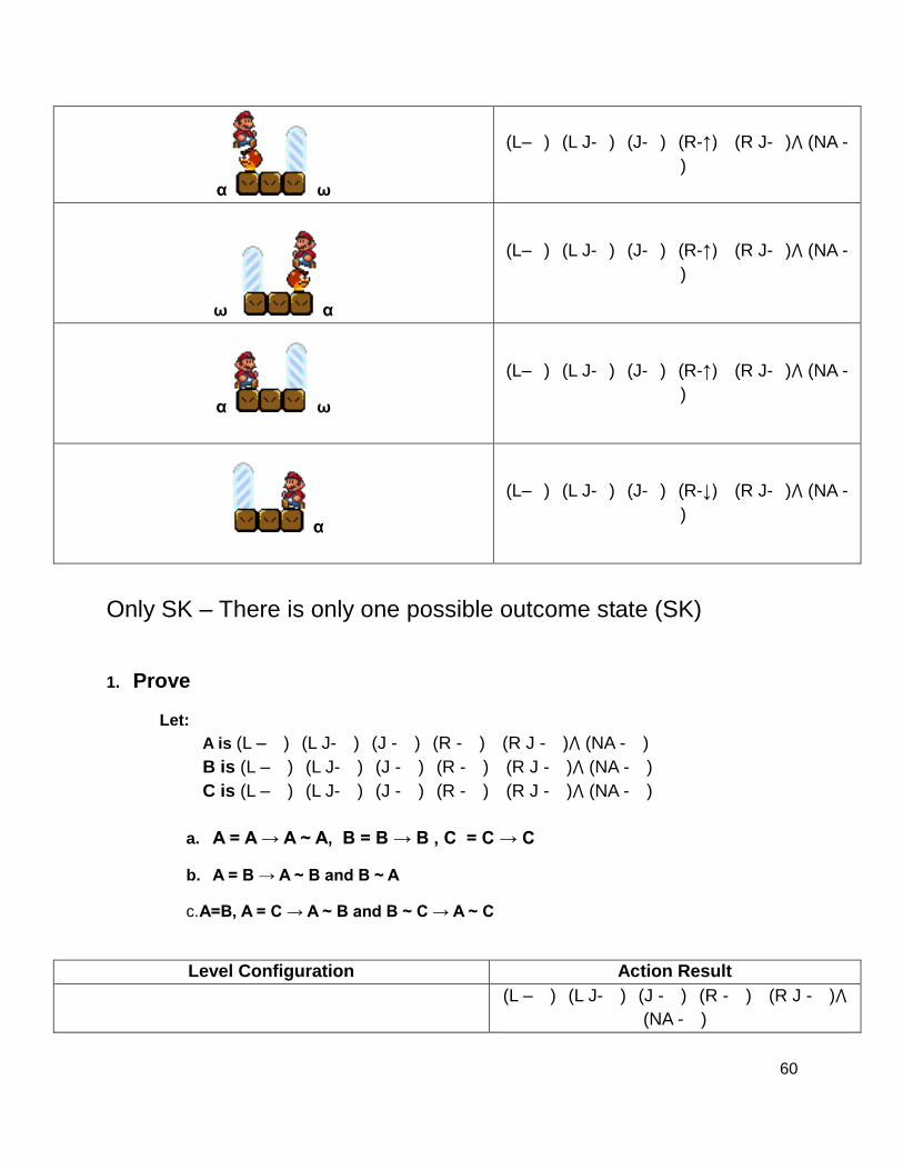
60

α ω

(L–�)�(L J-�)�(J-�)�(R-↑)� (R J-�)⋀ (NA -

�)

ω α

(L–�)�(L J-�)�(J-�)�(R-↑)� (R J-�)⋀ (NA -

�)

α ω

(L–�)�(L J-�)�(J-�)�(R-↑)� (R J-�)⋀ (NA -

�)

α

(L–�)�(L J-�)�(J-�)�(R-↓)� (R J-�)⋀ (NA -

�)

Only SK – There is only one possible outcome state (SK)

1. Prove

Let:

A is (L – �)�(L J- �)�(J - �)�(R - �)� (R J - �)⋀ (NA - �)

B is (L – �)�(L J- �)�(J - �)�(R - �)� (R J - �)⋀ (NA - �)

C is (L – �)�(L J- �)�(J - �)�(R - �)� (R J - �)⋀ (NA - �)

a. A = A → A ~ A, B = B → B , C = C → C

b. A = B → A ~ B and B ~ A

c. A=B, A = C → A ~ B and B ~ C → A ~ C

Level Configuration Action Result

(L – �)�(L J- �)�(J - �)�(R - �)� (R J - �)⋀

(NA - �)

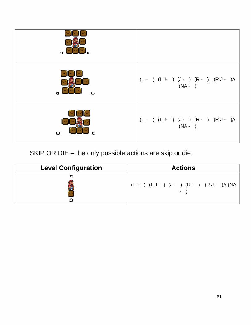
61

α ω

α ω

(L – �)�(L J- �)�(J - �)�(R - �)� (R J - �)⋀

(NA - �)

ω α

(L – �)�(L J- �)�(J - �)�(R - �)� (R J - �)⋀

(NA - �)

SKIP OR DIE – the only possible actions are skip or die

Level Configuration Actions

α

Ω

(L – �)�(L J- �)�(J - �)�(R - �)� (R J - �)⋀ (NA

- �)