Embed Size (px)
Citation preview

GEOPHYSICS, VOL. 63, NO. 3 (MAY-JUNE 1998); P. 826–840, 22 FIGS.
Marine magnetotellurics for petroleum exploration, Part II:Numerical analysis of subsalt resolution
G. Michael Hoversten∗, H. Frank Morrison∗, and Steven C. Constable‡
ABSTRACT
In areas where seismic imaging of the base of salt struc-tures is difficult, seaborne electromagnetic techniquesoffer complementary as well as independent structuralinformation. Numerical models of 2-D and 3-D salt struc-tures demonstrate the capability of the marine mag-netotelluric (MT) technique to map the base of thesalt structures with an average depth accuracy of bet-ter than 10%. The mapping of the base of the salt withmarine MT is virtually unaffected by internal varia-tion within the salt. Three-dimensional anticlinal struc-tures with a horizontal aspect ratio greater than twocan be interpreted adequately via two-dimensional in-versions. Marine MT can distinguish between salt struc-tures which possess deep vertical roots and those whichdo not.
One measure of the relative accuracy of MT and seis-mic methods can be made by considering the verticaland lateral position errors in the locations of interfacescaused by neglecting velocity anisotropy in migration.For the shallow part of the section where two-way traveltimes are on the order of 1 s, the vertical and lateral po-sition errors in the locations of salt-sediment interfacesfrom 2-D MT inversion is more than twice the expectedmigration error in reflectors in transversely isotropic sed-iments, such as those in the Gulf of Mexico. Deeper inthe section where two-way times are on the order of 4 s,lateral position errors in migration become comparableto those of the MT inverse, whereas seismic vertical po-sition errors remain more than a factor of two smallerthan MT errors. This analysis shows that structural map-ping accuracy would be improved using MT and seismictogether.
INTRODUCTION
Seismic imaging beneath high-velocity and often inhomo-geneous formations is a formidable task, even with the mostcomprehensive 3-D seismic surveying techniques. Basalts andcarbonates commonly pose difficulties for reflection surveysbecause excessive reverberations effectively mask reflectionsfrom structures beneath them. Similarly, salt structures containentrained sediments that produce significant scattering and, inaddition, have strong reflecting vertical boundaries that strainthe limits of 3-D migration. As a result, ambiguities in the in-terpretation of seismic reflection data often remain, even in3-D surveys. Finally, there are many practical exploration prob-lems where it is important to test a relatively simple hypothesisbefore deciding if the expense of a full 3-D seismic survey iswarranted.
Electrical resistivity provides important complementary in-formation in these situations. The resistivity of salt and ofbasalts and carbonates is often more than ten times greater
Presented at the 66th Annual International Meeting, Society of Exploration Geophysicists. Manuscript received by the Editor May 31, 1996; revisedmanuscript received March 31, 1997.∗Lawrence Berkeley Natl. Lab., 1 Cyclotron Road, Berkeley, CA 94720. E-mail: [email protected].; [email protected].‡Scripps Institution of Oceanography, IGPP 0025, 8604 La Jolla Shores Drive, LaJolla, CA 92093-0225; E-mail: [email protected]© 1998 Society of Exploration Geophysicists. All rights reserved.
than the surrounding sediments. With such contrasts, magne-totellurics (MT) can easily map major structures and resolvethe ambiguities noted above. In practice, the applicability ofMT spans the range from stand-alone techniques for resolvinggross structure to sophisticated joint applications where struc-ture derived from seismic is essential for fixing some of theparameters in the electrical model of the subsurface. The ef-fective resolution of MT depends entirely on the constraintsthat can be imposed on the interpretation by other data. In-terpreted alone, MT data can give only a gross description ofthe section. The more information that can be provided fromseismic data (for interface depths, location of faults, etc.), drill-hole data, or gravity, the better the accuracy of the resultingconductivity cross-section.
While marine MT can independently provide structural in-terpretations of lateral salt intrusions in the Gulf of Mexico(GOM) in seismic no-record areas, it is best used in conjunctionwith existing seismic data. The seismic data can define the struc-ture down to the top of the salt, allowing these parameters
826

Marine Magnetotellurics, Part 2 827
to be fixed at known values in the marine MT inversions, re-sulting in improved base salt structure. In deep explorationwhere velocity estimation for migration is inherently prob-lematic, the marine MT resistivity structure, when used withvelocity-resistivity relations derived from log information, canprovide independent velocity estimates that can constrain thepossible migration velocities.
Figure 1 shows a depth-converted seismic section for theGOM. In this example coherent reflections exist beneath thetop of the salt which can be interpreted, but uncertainty existsas to which reflector represents base of the salt. As we willdemonstrate, the accuracy of marine MT interpretations woulddetermine which seismic event corresponded to the base of thesalt.
The idea of using electromagnetic (EM) techniques, includ-ing MT, on the ocean bottom for petroleum exploration is notnew. Mobil Oil first tried MT in shallow water of the Gulf ofMexico in the late 1950s (Hoehn and Warner, 1960). The Mobilexperiment suffered from two major problems. First, the shal-low water depth of 20 m resulted in significant wave motion ofthe magnetic field sensors. Second, MT data processing in thelate ’50s did not use the remote reference techniques pioneeredby Gamble et al. (1979). The remote reference technique re-duces the systematic bias in impedance estimates. Controlled-source EM techniques have been studied for decades (e.g.,Chave et al., 1991; Constable et al., 1986; and Edwards, 1988)for probing the deep ocean crust and for their potential appli-cations for mineral and petroleum exploration. Studies of therelative effectiveness of controlled-source EM systems and ma-rine MT in terms of 2-D inverse model resolution of salt struc-tures has been presented by Hoversten (1992) and Hoverstenand Unsworth (1994). We focus on MT rather than controlledsource because we feel the logistics of using a controlled sourcewill result in higher survey costs compared to MT.
THE SYSTEM
A useful review of the general MT method is given by Vozoff(1991), and the effect of the sea water layer on impedance mea-surements on the ocean bottom is summarized in a companion
FIG. 1. Depth-converted seismic line from offshore GOM showing two possible base salt interpretations.
paper by Constable et al. (1998, this issue). The data used inour inversions are the apparent resistivity and phase definedfor a 1-D earth in Constable et al. (1998, this issue).
The source or incident fields for MT measurements in the10−3 to 1.0 Hz band (the frequencies of interest for marine MT)can be considered to be the horizontal components of the mag-netic field. All measured fields, electric E and magnetic H, canthen be considered to be produced by induction via linear trans-fer functions, T, from these horizontal components. In the mostgeneral case, within an inhomogeneous medium, these rela-tions can be written in the form of the matrix transfer function:
EObs.x
EObs.y
EObs.z
HObs.x
HObs.y
HObs.z
=
T1 T2
T3 T4
T5 T6
T7 T8
T9 T10
T11 T12
• HInc.x
HInc.y
(1)
Where HInc. represents the incident magnetic fields on thesea surface. One can form the two relations;
EObs.x
EObs.y
= T1 T2
T3 T4• HInc.
x
HInc.y
(2)
and
HObs.x
HObs.y
= T7 T8
T9 T10• HInc.
x
HInc.y
(3)
Rearranging equation (3) for the incident fields and substitut-ing into equation (2) yields:
EObs.x
EObs.y
= T1 T2
T3 T4• T7 T8
T9 T10
−1
• HObs.x
HObs.y
(4)

828 Hoversten et al.
Equation (4) shows that even within the medium, the orthog-onal E and H components can be related by a 2× 2 impedancetensor.
MT interpretation depends on the construction of models ofthe subsurface conductivity distribution which reproduce theobserved impedance (or, alternatively, the apparent resistivityand phase) at the measurement point. Papers by Smith andBooker (1988) and deGroot-Hedlin and Constable (1990) areexamples of numerical inversion processes for effecting thisinterpretation.
As pointed out in Part 1, Constable et al. (1998, this issue),if the section is horizontally layered, it is an interesting prop-erty of the plane-wave impedance that the ocean-bottomimpedance is the surface impedance of the earth, as if theocean were not present. If the earth is inhomogeneous, thisis not the case and the models and inversion codes must ac-count for the overlying ocean. We have used the general 2-Dcode of Wannamaker (1987), which generates impedances onthe ocean bottom.
MODELS AND MODELING
In this paper we will consider two sample models. The first isthe anticlinal structure shown in Figure 1. Seismic reflectionsmay or may not be evident from the base of the salt structure.When reflections are present, ambiguity may exist as to whichreflector represents the base of salt. Our first model introducesthe algorithms used and illustrates the resolution on the base ofthe salt for anticlinal structures. A second type of salt structureis that in which the presence or absence of a deep-seated rootis of critical interest. This problem is addressed by comparinginversions of a salt structure with and without a deep root.
A partial survey of deep induction logs from wells that pen-etrate salt in the GOM show sediment resistivities range from0.25 to 2 ohm-m while salt resistivities can range from 10 to1000 ohm-m. The low salt resistivities result from intermixingwith sediment during emplacement. The high salt resistivitiesrepresent massive salt. Figure 2 shows a portion of a typicaldeep induction log from a well penetrating salt in the GOM. Inall the models illustrated in this paper, we have used a sedimentresistivity of 1 ohm-m and a salt resistivity of 20 ohm-m.
The presence of oil in sediments raises their resistivity tobetween 10 and 20 ohm-m. If the salt acted as a structural trapwith oil just beneath the salt, the ability to distinguish betweensalt and oil-bearing sediment would be a problem. Fortunately,many if not all of the subsalt discoveries to date have involvedoil and gas located substantially below the salt, with a largeenough section of low-resistivity sediment beneath the salt toallow the base of salt to be distinguished.
The development of accurate numerical modeling algo-rithms for 2-D and 3-D structures has made great strides in thelast decade. It is now possible to calculate the MT response of1-D, 2-D, and 3-D structural models of interest to the petroleumindustry. In addition (2-D and 3-D) MT inverse technology isimproving rapidly. For the MT examples, we have used the for-ward 2-D MT modeling algorithm of Wannamaker (1987), theforward 3-D MT modeling algorithm of Mackie et al. (1993),and the 2-D MT inverse of deGroot-Hedlin and Constable(1990).
2-D salt anticline
Figure 3 shows a 2-D salt model whose style is taken from theseismic section of Figure 1. The sedimentary section is beneath
300 m of 0.3-ohm-m sea water. The slopes on either side ofthe anticline differ by a factor of two to investigate the lat-eral resolution of marine MT. The salt layer contains a randomdistribution of inclusions of both high and low resistivity rep-resenting zones of included sediment or massive salt. The MTapparent resistivity versus frequency for the model of Figure 3is compared to that for a homogeneous salt body with the samestructure in Figure 4 . Figure 4 demonstrates the insensitivity ofMT to variations in the resistivities within a resistive structuresuch as the salt. This occurs because the MT response at thesefrequencies is totally dominated by the effects of electric cur-rents channeled around the resistive salt and into the core ofthe anticline. There is very little change in response as the resis-tivity contrast between a resistive target and its surroundings
FIG. 2. Portion of a deep induction log from offshore GOMshowing salt and sediment resistivities.

Marine Magnetotellurics, Part 2 829
increases beyond a ratio of 10:1 because the contribution of in-duced currents within the resistive structure is negligible. Thisis very beneficial for the inversion of such data because internalvariations in the salt have little or no effect on the data.
SPATIAL VARIATIONS OF MAGNETIC FIELDSIN MARINE MT
Marine MT differs significantly from land MT if the sectionbelow the sea floor is inhomogeneous. At the air-ground inter-face the boundary condition requires that there be no verticalcomponent of current and consequently no vertical electric
FIG. 3. Two-dimensional numerical salt anticline model. Thesediment resistivity is 1 ohm-m and the salt resistivity is20 ohm-m. Within the salt structure are large inclusions, rang-ing in resistivity from 1 ohm-m representing sediment to100 ohm-m and representing nearly pure salt.
FIG. 4. TM mode (E field perpendicular to strike) apparentresistivity for 2-D anticline model shown in Figure 3 with andwithout the inclusions within the salt. Only a very minor dif-ference is caused by the inclusions beneath site 7.
field, Ez. This is not a requirement at the ocean bottom inter-face, so vertical electrical field measurement may be a usefuladditional measurement for marine MT. The presence of Ez,which varies spatially, also changes some assumptions aboutthe behavior of the horizontal magnetic fields in surface MTsurveys.
For example, in a 2-D medium in which the properties areconstant in the y-direction (the strike direction), a plane waveincident with a magnetic field polarized in the y-direction (theTM mode) must have a constant Hy value in the x-direction.This is a consequence of ∇̄ · H̄ = J̄, where J is current. Thevertical current, Jz, is given by
∂Hy
∂x− ∂Hx
∂y= Jz.
Since Hx is zero by definition of the incident field and Jz is zerofrom the boundary condition, Hy must be a constant. However,at the sea-floor interface Jz is not zero, so Hy can be a functionof x. On the sea floor then, both Hx and Hy are functions of posi-tion, even for 2-D geology. Profiling techniques such as electro-magnetic array profiling (EMAP) (Torres-Verdin and Bostick,1992), which are normally interpreted assuming transversemagnetic (TM) mode data with constant H,must be considereddifferently for sea-floor surveys.
To illustrate the magnitude of these new features of marineMT, we have calculated the transverse electric (TE) and TMmode apparent resistivities over the anticlinal model of Figure 3with and without the sea water layer. The ratio of TE apparentresistivity without sea water to the TE apparent resistivity withsea water is shown in the top panel of Figure 5, and the TM ap-parent resistivity ratio is shown in the bottom panel of Figure 5.The TM without/with anomaly is pronounced and reaches 18%over the anticline, while the maximum TE without/with ratiois only 2%.
When we consider the spatial variation across the anticlineof the Hy and Ex fields (TM impedance) caused by the sea wa-ter, we find that the maximum spatial variation in Hy acrossthe anticline is approximately 11% at 0.1 Hz. The Hy variationwith frequency decreases to approximately 5% at 0.001 Hz.The maximum spatial variation in Ex is approximately 10% at0.1 Hz and increases to nearly 15% at 0.001 Hz. This indicates(1) the variation of Hy due to the presence of the sea water is asignificant component in the differences in TM apparent resis-tivity shown in Figure 5 and (2) the common assumption thatboth horizontal components of H are for practical purposesconstant over the surface of a half-space is probably not safefor ocean bottom measurement.
SALT ANTICLINE
1-D inversion of 2-D salt anticline
Two-dimensional structures such as the one shown in Fig-ure 3 can be reasonably interpreted using 1-D inversion of themode in which E is parallel to strike (TE mode) because, withthe exception of the core of the anticline, the E parallel tostrike is only slightly perturbed from the 1-D response. Thetwo most popular techniques for 1-D inversion are (1) a least-squares inversion of a sparse layered model and (2) a smoothOccam inversion (Constable et al., 1987). Figure 6 shows a 1-DOccam model that fits the TE apparent resistivity and phase atsite 2 of the 2-D anticline model (without inclusions) shown in

830 Hoversten et al.
Figure 3. The 1-D Occam inversion assumes no prior knowl-edge about the model. The starting model is a half-space of1 ohm-m. The portion of the inverted model between 1000 and4000 m depth above 2 ohm-m represents the salt. However,two artificial high regions above and below the salt manifestthemselves in the unconstrained 1-D model.
Figure 7 shows the results of doing 1-D Occam inversions ofthe TE apparent resistivity and phase at all sites, separated by1 km, along the model shown in Figure 3 (without inclusions).On the flanks of the anticline, the 1-D models do a reasonablejob of imaging the base of the salt. However, at the core ofthe anticline where the TE currents are concentrated by thestructure, the TE apparent resistivities are elevated, resultingin 1-D models with a thicker section of high resistivity (salt)than is present in the 2-D model.
Smooth inverse models, whether 1-D or 2-D, have an in-herent drawback when used to interpret geology that containssharp discontinuities in physical properties. A resistivity con-tour must be picked to represent the location of the sharp phys-ical discontinuity, such as the base of the salt. The choice ofwhich resistivity contour to use must be guided by the inversion
FIG. 5. Numerical results of salt anticline model without sea water divided by results with sea water. Panels show the ratio of TE(a) and TM (b) apparent resistivities for the model shown in Figure 3 (no inclusions).
of numerical model data and by choosing the contour of theresulting inversions that most closely approximates the correctposition of the discontinuity.
For problems where information is available from other geo-physical methods, such as seismic or gravity, a technique thatcan accommodate this information as constraints on the inver-sion is preferable. A 1-D inversion that uses only three layersand in which the depth to the top of the salt and the resistivi-ties of the sediment and salt can be fixed yields a more accurateestimate of the salt thickness. Figure 8 presents the three-layer1-D inversion of the 2-D salt anticline model. The average er-ror in the depth to the base of the salt beneath the MT sitesis 13.2% for the three-layer inversions shown in Figure 8 and16.2% for the Occam inversions shown in Figure 7. In addition,the three-layer inversion error in the anticline apex thicknessis 10% better than the unconstrained Occam estimate.
2-D inversions of 2-D salt anticline
While the 1-D inversions can be used as a fast first pass atdata modeling, additional accuracy can be gained by using a

Marine Magnetotellurics, Part 2 831
full 2-D solution. The 2-D inversions were done assuming thestructure to the top of the salt would be constrained by seismicdata; hence, the resistivity and structure were held constantto the top of the salt. The starting model was a half-space of1 ohm-m sediment with 300 m of overlying sea water.
For 3-D structures, which have surface topography out of theplane of a 2-D inversion, fixing the top structure may actuallydegrade the accuracy of the base salt from a 2-D inversion. Theappropriateness of fixing the top structure is model dependentand must be judged based on modeling results for a particularsituation.
Thirteen MT sites, spaced 1 km apart, were used with tenequally spaced frequencies in the log10 domain from 1.0 to0.001 Hz. Figure 9 shows the MT inverse model when bothTE and TM mode apparent resistivity and phase data wereused with 5% random noise added. The true model structure isshown in white. To quantitatively interpret the inverse modelsfor the base of the salt, a resistivity contour which most closelymatches the true base of salt must be chosen—in this example,the 3.2-ohm-m contour. The percent error plotted in the toppanel of Figure 9 is the percent difference between the truemodel and the depths of the 3.2 ohm-m contour, shown in themiddle panel, calculated at the MT sites. The errors on theflanks of the anticline are near 5%. Across the apex of thestructure they increase to a maximum of 14%. The averagebase salt depth error is 8% across the entire model.
The bottom panel of Figure 9 shows the complete smoothresistivity distribution recovered by the Occam 2-D inversion.The granularity of the resistivity represents the size of the
FIG. 6. One-dimensional Occam inversion of TE (E parallel tostrike) at site 2 of the salt anticline model without inclusionsshown in Figure 3.
regularization mesh, which defines the blocks of constant resis-tivity which are the inversion parameters. The regularizationmesh was generated without any attempt to match regular-ization mesh boundaries to boundaries in the true model. Asa result, most of the regularization mesh blocks straddle thesalt-sediment boundaries in the true model. An exception oc-curs beneath site 6, where the regularization mesh boundaryfalls within 100 m of the true model boundary. At this locationthe error is a minimum. In general, the depth of the 3.2 ohm-mcontour is within one regularization mesh block of the truedepth.
The observed and calculated TE and TM apparent resistiv-ity data for the 2-D inversion shown in Figure 9 is shown inFigure 10. The area of greatest data misfit occurs at the apexof the anticline in the TE mode around 0.02 Hz where the TEapparent resistivity is most distorted by the 5% random noise.This translates into the increased base salt errors seen in the
FIG. 7. (c) The stitched-together Occam 1-D TE mode inver-sions of Figure 3 data without inclusions and with 5% ran-dom noise added. (a) Error in the base salt estimates when the2-ohm-m contour (shown in the middle panel) of the smoothed1-D models is chosen as the base salt.
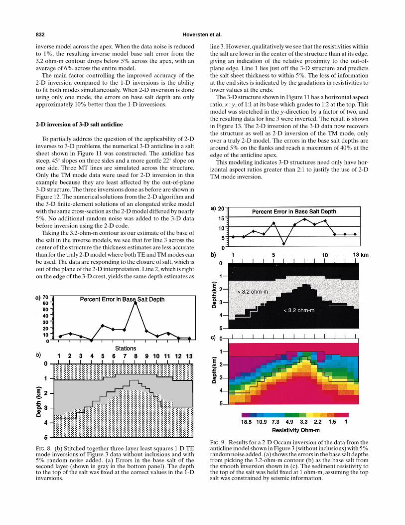
832 Hoversten et al.
inverse model across the apex. When the data noise is reducedto 1%, the resulting inverse model base salt error from the3.2 ohm-m contour drops below 5% across the apex, with anaverage of 6% across the entire model.
The main factor controlling the improved accuracy of the2-D inversion compared to the 1-D inversions is the abilityto fit both modes simultaneously. When 2-D inversion is doneusing only one mode, the errors on base salt depth are onlyapproximately 10% better than the 1-D inversions.
2-D inversion of 3-D salt anticline
To partially address the question of the applicability of 2-Dinverses to 3-D problems, the numerical 3-D anticline in a saltsheet shown in Figure 11 was constructed. The anticline hassteep, 45◦ slopes on three sides and a more gentle 22◦ slope onone side. Three MT lines are simulated across the structure.Only the TM mode data were used for 2-D inversion in thisexample because they are least affected by the out-of-plane3-D structure. The three inversions done as before are shown inFigure 12. The numerical solutions from the 2-D algorithm andthe 3-D finite-element solutions of an elongated strike modelwith the same cross-section as the 2-D model differed by nearly5%. No additional random noise was added to the 3-D databefore inversion using the 2-D code.
Taking the 3.2-ohm-m contour as our estimate of the base ofthe salt in the inverse models, we see that for line 3 across thecenter of the structure the thickness estimates are less accuratethan for the truly 2-D model where both TE and TM modes canbe used. The data are responding to the closure of salt, which isout of the plane of the 2-D interpretation. Line 2, which is righton the edge of the 3-D crest, yields the same depth estimates as
FIG. 8. (b) Stitched-together three-layer least squares 1-D TEmode inversions of Figure 3 data without inclusions and with5% random noise added. (a) Errors in the base salt of thesecond layer (shown in gray in the bottom panel). The depthto the top of the salt was fixed at the correct values in the 1-Dinversions.
line 3. However, qualitatively we see that the resistivities withinthe salt are lower in the center of the structure than at its edge,giving an indication of the relative proximity to the out-of-plane edge. Line 1 lies just off the 3-D structure and predictsthe salt sheet thickness to within 5%. The loss of informationat the end sites is indicated by the gradations in resistivities tolower values at the ends.
The 3-D structure shown in Figure 11 has a horizontal aspectratio, x : y, of 1:1 at its base which grades to 1:2 at the top. Thismodel was stretched in the y-direction by a factor of two, andthe resulting data for line 3 were inverted. The result is shownin Figure 13. The 2-D inversion of the 3-D data now recoversthe structure as well as 2-D inversion of the TM mode, onlyover a truly 2-D model. The errors in the base salt depths arearound 5% on the flanks and reach a maximum of 40% at theedge of the anticline apex.
This modeling indicates 3-D structures need only have hor-izontal aspect ratios greater than 2:1 to justify the use of 2-DTM mode inversion.
FIG. 9. Results for a 2-D Occam inversion of the data from theanticline model shown in Figure 3 (without inclusions) with 5%random noise added. (a) shows the errors in the base salt depthsfrom picking the 3.2-ohm-m contour (b) as the base salt fromthe smooth inversion shown in (c). The sediment resistivity tothe top of the salt was held fixed at 1 ohm-m, assuming the topsalt was constrained by seismic information.

Marine Magnetotellurics, Part 2 833
ROOTED SALT STRUCTURE
TE and TM mode responses of rooted salt structure
A second problem of interest is whether a particular saltstructure possesses a deep root. The question of the presenceof a root can be difficult to answer with seismic data becausethe overlying salt intrusion can mask the signature of the rootas well as the signature of terminating beds. In addition, rootswith near-vertical walls yield a seismic response that requiresextremely long offsets for migration to correctly position thenear-vertical reflectors. The use of gravity data can also be prob-lematic if the salt-sediment density crossover point falls within
FIG. 10. Computed and observed TE and TM apparent resistivities for the inversion shown in Figure 9. (a) Observed TE apparentresistivity; numerical data from the model in Figure 3 without inclusions and with 5% random noise added. (b) Observed TMapparent resistivity; numerical data with 5% random noise added. (c) Calculated TE apparent resistivity for the inverse modelshown in Figure 9. (d) Calculated TM apparent resistivity for the inverse model shown in Figure 9.
the depth range of the root. In cases where seismic and gravityprovide ambiguous interpretations of deep root structures, ma-rine MT can provide an additional independent interpretation.
We constructed 2-D and 3-D versions of a salt structure withand without a deep root. The model is taken from an actualstructure in the Gulf of Mexico. The cross-section of the struc-ture in the x-zplane is outlined in black in Figure 15. Three 3-Dversions of this model were constructed with strike lengths of24, 16, and 12 km, respectively, in the y-direction. Before con-sidering the 2-D inversions of the numerical data, we will con-sider some aspects of the MT response of such a structure. Wewill refer to two portions of the structure by name. The portion

834 Hoversten et al.
between 3 and 5 km depth and −12 to +2 km in X will be re-ferred to as the sill and the portion below 5 km depth will bereferred to as the root.
The TM (Zxy) and TE (Zyx) apparent resistivities for the 2-Dversion of the rooted and rootless salt structure are shown inFigure 14. There are three main points to be noticed regardingthe response of the rooted and the rootless models:
1) The magnitude of the TM response is approximately fivetimes larger than the TE response.
2) The TE response is more sensitive to the presence of thesill portion of the structure. This is shown by the spatialvariation of the TE apparent resistivity and phase (notshown) between −10 and 0 km as compared to the TMmode data.
3) The TE response is almost completely insensitive to theroot, as seen by comparing Figures 14c and 14d.
2-D inversion of 2-D rooted salt structure
The 2-D inversions of the rooted and rootless salt modeldata were done in the same manner as the 2-D anticline ex-amples. Only the portion of the model below the top of thesalt was inverted. All data had 5% Gaussian random noiseadded, and the inversions were all started from a 1-ohm-mhalf-space. Both TE and TM mode apparent resistivity and
FIG. 11. Three-dimensional salt anticline model. (a) Plane viewof structure. (b) Cross-section view. Numerical data were gen-erated along three lines marked lines 1 through 3 for inversionusing the 2-D Occam inverse.
phase was used at ten frequencies equally spaced in log10 from1 to 0.001 Hz. The inversion blocks of the model were 0.5 kmwide and deep, equal to one-half a station separation, just be-neath the top of the salt. Their width remained constant overthe depth range of the structure, but their thickness increasedwith depth. Figure 15 shows the 2-D Occam inversion of therootless structure; Figure 16 shows the 2-D Occam inversionof the rooted structure.
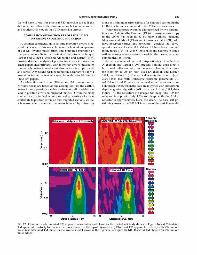
The outline of the rooted salt structure is overlaid in blackon both figures. The lower panel has the 2-D Occam inversionof the 5% noise data as resistivity above and below 3.4 ohm-m.The upper panel shows the actual smooth Occam 2-D inversemodel. The observed (numerical + 5% Gaussian noise) andcalculated TM apparent resistivity and phase are shown inFigure 17 for the final inverse model with an rms misfit of 1.0.The TE mode data fits are comparable.
The 2-D inversions of rooted and rootless models show anumber of things. First, the difference in the inverse modelsshown in Figures 15 (no root) and 16 (rooted) is a strikingindication that the presence or absence of a deep root can be
FIG. 12. Two-dimensional Occam inversion models of TMmode only for lines 1 through 3 shown in Figure 11. (a) Line 1.(b) Line 2. (c) Line 3. (d) Percent error in the depth of the basesalt on lines 2 and 3 from picking the 3.2-ohm-m contour ofinverse models as the base salt.

Marine Magnetotellurics, Part 2 835
FIG. 13. Two-dimensional Occam inversion models of the TMmode only for line 3 of the model shown in Figure 11 when themodel is stretched by a factor of two perpendicular to line 3. (a)Percent error in the depth of the base salt when the 3.2-ohm-mcontour of the inversion model is interpreted as the base salt.(b) Occam 2-D smooth resistivity inversion of line 3 for thestretched model.
FIG. 14. TE and TM mode apparent resistivity for the salt root model with and without the root. (a) Rooted TM response. (b)Rootless TM response. (c) Rooted TE response. (d) Rootless TE response. Rooted and rootless responses use common color scalesshown in the rootless panels.
determined by marine MT. Second, resolution of the upperpart of the structure (above 5 km depth) is very good, withthe maximum error of 1 km below the −5 km surface locationfor the rooted model and about 0.5 km for the rootless model.Third, both the rooted and rootless models show anomalouslow-resistivity zones (0.3 to 0.5 ohm-m) beneath the salt sill.
To demonstrate the importance of the TE mode data tomodel resolution, inversions of the rooted and rootless TMmode data with 5% Gaussian noise were done as before. Theinversion results for the rootless model are shown in Figure 18,and the rooted inversions are shown in Figure 19. While thepresence or absence of a deep root can be seen clearly in theinversions, the resolution of the salt sill between 3 and 5 kmdepth is much poorer without the TE data. Without the dataredundancy of the TE mode, noise in the remaining TM datahas a larger impact on the inverted model, causing the low-resistivity zones in the shallow part of the salt below 2.5 and5 km on the horizontal axis. In addition, the deep root is lesswell defined using the TM data only.
The benefit of TE for resolving the root comes from its lackof response to the root. This at first seems contradictory untilone realizes that only relatively thin (in the in-line direction)resistive roots will produce no TE response while fitting theTM response. Without the TE, the root structures can becomemuch wider with depth and still fit the TM mode data alone.

836 Hoversten et al.
2-D inversion of 3-D rooted salt structure
The question naturally arises as to the effect of strike lengthon the response of a structure such as the rooted model shownin Figure 16. To address this, we ran a series of 3-D versions ofthe rooted and rootless models where the strike length in theout-of-plane (y) direction ranged from 24 to 12 km. For thismodel, a strike length of 12 km represents a limit at which the2-D inversions can distinguish the presence or absence of theroot. The strike length of 12 km is approximately one-half themodel’s length in the observation line direction. The observa-tion lines were at y = 0, with the salt extending equal amountsin the positive and negative y-directions. Figures 20 and 21show the 2-D Occam inversion of the rootless and rooted 3-Dmodel data, respectively. Both TE (E parallel to y) and TM (Eperpendicular to y) modes were used with 5% Gaussian noiseadded. The 2-D inversion produces models with lower average
FIG. 15. Occam 2-D inversion of a 2-D salt structure withouta deep root. Inversion used both TE and TM mode apparentresistivity and phase at ten frequencies evenly spaced in log10
between 0.001 and 1 Hz. The salt with the root is outlinedin black. Sediment resistivity is 1 ohm-m; salt resistivity is 20ohm-m. (a) Smooth inversion model resistivities. (b) Resistiv-ities greater than 3.4 ohm-m are shown in dark blue.
resistivities compared to the models found for purely 2-D data.This results in the lower threshold value of 1.5 ohm-m used inthe bottom panels of these plots compared to the 3.4 ohm-mused in the inversion of 2-D data. The distinction betweenrooted and rootless models, while present, is small and unclearevidence for the presence or absence of a root.
Three-dimensional models with a strike length of 16 km yield2-D inversions which are significantly different and can dis-tinguish between the rooted and rootless models. Also, if theadded noise is reduced to 2% for the 12-km strike length 3-Dmodels, the 2-D inversions yield results which would distin-guish between rooted and rootless versions. Although the 2-Dinversion of the 3-D rooted and rootless models with a 12-kmstrike length differ only slightly, the 3-D data still have sig-nificant differences between models. The TM (Zxy) apparentresistivity is elevated by 25% at 0.001 Hz and 15% at 0.01 Hz bythe presence of the root compared to the rootless 3-D model.
FIG. 16. Occam 2-D inversion of a 2-D salt structure with adeep root. Inversion used both TE and TM mode apparentresistivity and phase at ten frequencies evenly spaced in log10
between 0.001 and 1 Hz. The outline of the salt is shown in blackSediment resistivity is 1 ohm-m; Salt resistivity is 20 ohm-m.(a) Smooth inversion model resistivities. (b) Inversion modelresistivities greater than 3.4 ohm-m.
Marine Magnetotellurics, Part 2 837
We will have to wait for practical 3-D inversion to see if thisdifference will allow better discrimination between the rootedand rootless 3-D models than 2-D inversion affords.
COMPARISON OF POSITION ERRORS FOR 2-D MTINVERSION AND SEISMIC MIGRATION
A detailed consideration of seismic migration errors is be-yond the scope of this work; however, a limited comparisonof our MT inverse model errors and computed migration er-rors puts our results in the context of the seismic technique.Larner and Cohen (1993) and Alkhalifah and Larner (1994)provide detailed analysis of positioning errors in migration.Their papers deal primarily with migration errors induced bytransversely isotropic media but also contain isotropic mediaas a subset. Any reader wishing to put the accuracy of our MTinversions in the context of a specific model should refer tothese two papers.
As Alkhalifah and Larner (1994) state, “Most migration al-gorithms today are based on the assumption that the earth isisotropic, an approximation that is often not valid and thus canlead to position errors on migrated images.” Given the manysources of error in field acquisition and processing which cancontribute to position errors on final migrated sections, we feelit is reasonable to consider the errors induced by anisotropy
FIG. 17. Observed and computed TM apparent resistivities and phase for the rooted salt body shown in Figure 16. (a) CalculatedTM apparent resistivity for the inverse model shown in the top of Figure 16. (b) Observed TM apparent resistivity with 5% randomnoise. (c) Calculated TM phase for the inverse model shown in the top panel of Figure 16. (d) Observed TM phase with 5% randomnoise added.
alone as a minimum error estimate for migrated sections in theGOM which can be compared to the MT inversion errors.
Transverse anisotropy can be characterized by two parame-ters, ε and δ, defined by Thomsen (1986). Transverse anisotropyin the GOM has been noted by many authors, includingMeadows and Abriel (1994) and Gonzolez et al. (1991), whohave observed vertical and horizontal velocities that corre-spond to values of ε near 0.1. Values of δ have been observedin the range of 0.1 to 0.3 in GOM shales and near 0.0 in sands,with increasing values as a function of depth (Larner, personalcommunication, 1996).
As an example of vertical mispositioning of reflectors,Alkhalifah and Larner (1994) present a model consisting ofhorizontal reflectors with end segments having dips rang-ing from 30◦ to 90◦ on both sides (Alkhalifah and Larner,1994, their Figure 10). The vertical velocity function is v(z)=2000+ 0.6z m/s with transverse isotropic parameters δ=−0.035 and ε= 0.11, which correspond to the Taylor sandstone(Thomsen, 1986). When the data are migrated with an isotropicdepth migration algorithm (Alkhalifah and Larner, 1994, theirFigure 13), the reflectors are imaged too deep. The 1.25-kmreflector is approximately 3.5% too deep, while the 3.0-kmreflector is approximately 6.5% too deep. The base salt po-sitioning errors in the 2-D MT inversion of the anticline model

838 Hoversten et al.
(Figure 9) range from 5% on the flanks where the structure ishorizontal to 14% at the apex of the anticline.
Horizontal positioning of near-vertical reflectors in migra-tion has inherently more uncertainty than vertical positioning.If we consider the horizontal position of the edges of the deepsalt root shown in Figure 16 in the depth range of 5 to 9 km,this corresponds to a two-way time range of 2.8 to 3.8 s for thev(z)= 2000+ 0.6zm/s velocity function. Alkhalifah and Larner(1994) present the position error as a function of dip angle fortwo-way times of 1, 2, 3, and 4 s for ε= 0.1 and a range of δ. Theyplot the position errors as a function of horizontal wavelengthafter migration. We have used a slope [p in equation (16) ofLarner and Cohen (1993)] of 0.75 s/km as appropriate for theGOM, taken from Figure 7a of Hale et al. (1992), to computethe horizontal wavelength before migration to convert valuesfrom Alkhalifah and Larner (1994, their Figure 6) into me-ters. Figure 22 shows the lateral position errors after migrationfor a vertical reflector (dip= 90◦) for δ= 0.0, appropriate for
FIG. 18. Occam 2-D inversion of a 2-D salt structure without adeep root. Inversion used only TM mode apparent resistivityand phase at ten frequencies evenly spaced in log10 between0.001 and 1 Hz. The salt with the root is outlined in black.Sediment resistivity is 1 ohm-m; salt resistivity is 20 ohm-m. (a)Smooth inversion model resistivities. (b) Resistivities greaterthan 3.4 ohm-m are shown in dark blue.
sand, and δ= 0.1, appropriate for shale at dominant frequen-cies of 20 and 30 Hz. The figure shows that the lateral positionerrors in the shallower section around 1 s two-way time aresmall—on the order of 50 m. However, at a two-way time of 3 san error near 350 m results in shale; an error of 200 m resultsin sand at 30 Hz. At 4 s the error in shale at 20 Hz is nearly1 km. The migration errors from Figure 22 at the top of theroot structure (two-way time of 3 s) shown in Figure 15 areless than half the error in the horizontal position of the leftside of the root from the MT inversion. However, the errors inmigration and the accuracy of MT become comparable at thebase of the structure. This comparison strongly suggests that ajoint inversion of seismic and MT, each depending on differentphysical properties, would yield more accurate locations forsubsalt structures.
In many exploration situations where well data are available,migration parameters can be tuned more finely by trial and er-ror, resulting in more accurate migrations than the examples
FIG. 19. Occam 2-D inversion of a 2-D salt structure with adeep root. Inversion used only TM mode apparent resistivityand phase at ten frequencies evenly spaced in log10 between0.001 and 1 Hz. The salt is outlined in black. Sediment re-sistivity is 1 ohm-m; salt resistivity is 20 ohm-m. (a) Smoothinversion model resistivities. (b) Inversion model resistivitiesgreater than 3.4 ohm-m.

Marine Magnetotellurics, Part 2 839
considered here. However, these examples can be consideredwithin the range of errors expected in the GOM for rank ex-ploration where no other data exist. Furthermore, in rank ex-plorations it is unlikely that full 3-D data and prestack-depthmigration would be used. In rank exploration where knowledgeof transverse anisotropy is not available, the information avail-able from MT regarding salt-sediment contacts is expected tobe similar to that provided by reconnaissance 2-D seismic.
FUTURE WORK
The current work is far from a complete study of the po-tential application of marine MT for mapping salt or anyhigh-velocity, high-resistivity structure. The current study high-lights the difficulties of using smooth inverse models to in-terpret sharp discontinuities in physical properties, such asoccur in resistivity at salt-sediment contacts. A better approachwould be to use an inversion scheme that includes the abilityto accommodate sharp discontinuities in the inverse model.
FIG. 20. Occam 2-D inversion of a 3-D salt structure withouta deep root. The structure is 12 km long in the out-of-planedirection. The observed data are from a line at the midpoint inthe bodies’ strike extent. Inversion used TE (Zyx) and TM (Zxy)mode apparent resistivity and phase at ten frequencies evenlyspaced in log10 between 0.001 and 1 Hz. The salt with the root isoutlined in black. (a) Smooth inversion model resistivities. (b)Resistivities greater than 1.5 ohm-m are shown in dark blue.
Work is currently under way to refine a new 2-D MT in-verse algorithm parameterized by variable thickness layers andpolygonal regions whose boundary locations are the inverseparameters. Additionally, there is a need for 3-D MT inversioncapabilities.
CONCLUSIONS
Based on numerical modeling, marine MT can map the baseof anticlinal features in lateral salt intrusions to within an aver-age depth accuracy of better than 10%. Vertical resolution onsalt thickness is lost for salt thinner than approximately one-tenth of a plane wave skin depth at the highest frequency thatresponds to the salt presence. The lateral resolution is compa-rable to the vertical resolution. Different slopes on the oppositesides of the model anticlines were clearly mapped by the 2-D in-versions. The maximum errors in salt anticline thickness occurfor both 1-D and 2-D MT inversions at the apex of anticlineswhere the salt thickness was only 400 m. Two-dimensional MTinversion using both TE and TM modes resolves the anticline
FIG. 21. Occam 2-D inversion of a 3-D salt structure with adeep root. The structure is 12 km long in the out-of-plane di-rection. The observed data are from a line at the midpoint in thebodies’ strike extent. Inversion used TE (Zyx) and TM (Zxy)mode apparent resistivity and phase at ten frequencies evenlyspaced in log10 between 0.001 and 1 Hz. The salt with the root isoutlined in black. (a) Smooth inversion model resistivities. (b)Resistivities greater than 1.5 ohm-m are shown in dark blue.

840 Hoversten et al.
FIG. 22. Lateral positions errors for a vertical reflector whenvelocity anisotropy is neglected in migration. Taken fromAlkhalifah and Larner (1994, their Figure 6) for δ= 0.0, ap-propriate for sand, and δ= 0.1, appropriate for shale at dom-inant frequencies of 20 and 30 Hz. Vertical velocity function:v(z)= 2000+ 0.6z m/s velocity. A slope [p in equation (16) ofLarner and Cohen (1993)] of 0.75 s/km, taken from Figure 7aof Hale et al. (1992), was used to compute the horizontal wave-length before migration to convert values from Alkhalifah andLarner’s Figure 6 (1994) into meters.
apex thickness to within 14%. Two-dimensional inversion of3-D numerical data indicates that as long as the horizontal as-pect ratio of a 3-D anticline is greater than two, the inversionaccuracy is comparable to the accuracy of inverting truly 2-Ddata except at the apex. Three-dimensional anticline thicknessestimates via 2-D inversion of TM mode data at the apex iscomparable to the accuracy of 2-D inversion of truly 2-D datausing only the TM mode. Although the quantitative measureof picking a single resistivity contour produced roughly 50%errors at the apex for the 3-D model, resistivities were reducedcompared to the areas of thicker salt on either side, giving aqualitative measure of the salt thinning. Finally, the marineMT data can distinguish between those models which possessa deep root structure and those which do not.
The most important conclusion from this study is that MTcan provide valuable complementary data to resolve velocityambiguities that cause significant positioning errors in migrated
seismic data. The fact that realistic anisotropies can causemispositioning errors which are a significant fraction of MTinversion errors indicates that if the two data sets were inter-preted together, the absolute error in the location of interfacescould be reduced.
ACKNOWLEDGMENTS
We would like to thank corporate sponsors AGIP, BP, BHP,British Gas, Chevron, Texaco, and Western Atlas in coopera-tion with the U.S. Dept. of Energy, Office of Energy Research,Office of Computational and Technology Research, Labora-tory Technology Applications Division, under Contract No.DE-AC03-76SF00098.
REFERENCES
Alkhalifah, T., and Larner, K., 1994, Migration error in transverselyisotropic media: Geophysics, 59, 1405–1418.
Chave, A. D., Constable, S. C., and Edwards, R. N., 1991, Electri-cal exploration methods for the seafloor, in Nabighian, M. N., Ed.,Electromagnetic methods in applied geophysics, 2: Soc. Expl. Geo-phys., 931–969.
Constable, S. C., Cox, C. S., and Chave, A. D., 1986, Offshore electro-magnetic surveying techniques: 56th Ann. Internat. Mtg., Soc. Expl.Geophys., Expanded Abstracts.
Constable, S. C., Parker, R. L., and Constable, C. G., 1987, Occam’sinversion—a practical algorithm for generating smooth models fromelectromagnetic sounding data: Geophysics, 52, 289–300.
Edwards, R. N., 1988, Two-dimensional modeling of a towed in-lineelectric dipole-dipole sea-floor electromagnetic system—the opti-mum time delay or frequency for target resolution: Geophysics, 53,846–853.
Gamble, T. D., Goubau, W. M., and Clarke, J., 1979, Magnetotelluricswith a remote magnetic reference: Geophysics, 44, 53–68.
Gonzalez, A., Lynn, W., and Robinson, W. F., 1991, Prestack frequency-wavenumber ( f -k) migration in transversely isotropic media: 61stAnn. Internat. Mtg., Soc. Expl. Geophys., Expanded Abstracts,1155–1157.
deGroot-Hedlin, C., and Constable, S., 1990, Occam’s inversion to gen-erate smooth, two-dimensional models from magnetotelluric data:Geophysics, 55, 1613–1624.
Hale, D., Hill, N. R., and Stefani, J., 1992, Imaging salt with turningseismic waves: Geophysics, 57, 1453–1462.
Hoehn, G. L., and Warner, B. N., 1960, Magnetotelluric measurementsin the Gulf of Mexico at 20m ocean depths, in Handbook of geo-physical exploration at sea: CRC, 397–416.
Hoversten, G. M., 1992, Seaborne electromagnetic subsalt exploration:EOS, 73, No. 43, Suppl., 313.
Hoversten, G. M., and Unsworth, M., 1994, Subsalt imaging viaseaborne electromagnetics: Proc. Offshore Tech. Conf., 26, 231–240.
Larner, K. L., and Cohen, J. K., 1993, Migration error in transverselyisotropic media with linear velocity variation in depth: Geophysics,58, 1454–1467.
Mackie, R. L., Madden, T. R., and Wannamaker, P. E., 1993, Three-dimensional magnetotelluric modeling using difference equations—Theory and solutions: Geophysics, 58, 215–226.
Meadows, M. A., and Abriel, W. L., 1994, 3-D poststack phase-shiftmigration in transversely isotropic media: 64th Ann. Internat. Mtg.,Soc. Expl. Geophys., Expanded Abstracts, 1205–1208.
Smith, J. T., and Booker, J. R., 1988, Magnetotelluric inversion forminimum structure: Geophysics, 53, 1565–1576.
Thomsen, L., 1986, Weak elastic anisotropy: Geophysics, 51, 1954–1966.
Torres-Verdin, C., and Bostick, F. X., Jr., 1992, Principles of spatialsurface electric field filtering in magnetotellurics: Electromagneticarray profiling (EMAP): Geophysics, 57, 603–622.
Wannamaker, P. E., Stodt, J. A., and Rijo, L., 1987, A stable finite-element solution for two-dimensional magnetotelluric modeling:Geophys. J. Roy. Astr. Soc., 88, 277–296.
Vozoff, K., 1991, The magnetotelluric method, in Nabighian, M. N.,Ed., Electromagnetic methods in applied geophysics, 2: Soc. Expl.Geophys., 641–711.


![[Chap6102]CHAPTER 61:02 PETROLEUM … · PETROLEUM (EXPLORATION AND PRODUCTION) ARRANGEMENT OF ... Notice of intention to commence exploration or ... Commissioner for Petroleum Exploration](https://img.pdfslide.us/doc/110x75/5b7bb8197f8b9adb4c8d3af1/chap6102chapter-6102-petroleum-petroleum-exploration-and-production-arrangement.jpg)