See discussions, stats, and author profiles for this publication at: https://www.researchgate.net/publication/323012396

Marine heatwaves off eastern Tasmania: Trends, interannual variability, and

predictability

Article  in  Progress In Oceanography · February 2018

DOI: 10.1016/j.pocean.2018.02.007

CITATIONS

15READS

522

6 authors, including:

Some of the authors of this publication are also working on these related projects:

Enabling adaptation pathways View project

World Harbour Project View project

Eric C. J. Oliver

Dalhousie University

58 PUBLICATIONS   1,138 CITATIONS   

SEE PROFILE

Alistair J. Hobday

The Commonwealth Scientific and Industrial Research Organisation

370 PUBLICATIONS   12,838 CITATIONS   

SEE PROFILE

Neil J. Holbrook

University of Tasmania

118 PUBLICATIONS   4,121 CITATIONS   

SEE PROFILE

Scott D. Ling

University of Tasmania

73 PUBLICATIONS   3,396 CITATIONS   

SEE PROFILE

All content following this page was uploaded by Eric C. J. Oliver on 08 March 2018.

The user has requested enhancement of the downloaded file.

Contents lists available at ScienceDirect

Progress in Oceanography

journal homepage: www.elsevier.com/locate/pocean

Marine heatwaves off eastern Tasmania: Trends, interannual variability, andpredictability

Eric C.J. Olivera,b,c,⁎, Véronique Lagoa,b,d, Alistair J. Hobdayd, Neil J. Holbrooka,e, Scott D. Linga,Craig N. Mundya

a Institute for Marine and Antarctic Studies, University of Tasmania, Hobart, Tasmania, AustraliabAustralian Research Council Centre of Excellence for Climate System Science, University of Tasmania, Hobart, Tasmania, Australiac Department of Oceanography, Dalhousie University, Halifax, Nova Scotia, Canadad CSIRO Oceans and Atmosphere, Hobart, Tasmania, Australiae Australian Research Council Centre of Excellence for Climate Extremes, University of Tasmania, Hobart, Tasmania, Australia

A R T I C L E I N F O

Keywords:Extreme eventsClimate changeClimate variabilityOcean modellingSelf-organising maps

A B S T R A C T

Surface waters off eastern Tasmania are a global warming hotspot. Here, mean temperatures have been risingover several decades at nearly four times the global average rate, with concomitant changes in extreme tem-peratures – marine heatwaves. These changes have recently caused the marine biodiversity, fisheries andaquaculture industries off Tasmania’s east coast to come under stress. In this study we quantify the long-termtrends, variability and predictability of marine heatwaves off eastern Tasmania. We use a high-resolution oceanmodel for Tasmania’s eastern continental shelf. The ocean state over the 1993–2015 period is hindcast, pro-viding daily estimates of the three-dimensional temperature and circulation fields. Marine heatwaves areidentified at the surface and subsurface from ocean temperature time series using a consistent definition. Trendsin marine heatwave frequency are positive nearly everywhere and annual marine heatwave days and penetrationdepths indicate significant positive changes, particularly off southeastern Tasmania. A decomposition into modesof variability indicates that the East Australian Current is the dominant driver of marine heatwaves across thedomain. Self-organising maps are used to identify 12 marine heatwave types, each with its own regionality,seasonality, and associated large-scale oceanic and atmospheric circulation patterns. The implications of thiswork for marine ecosystems and their management were revealed through review of past impacts and stake-holder discussions regarding use of these data.

1. Introduction

Heatwaves are major climate extremes, in both the atmosphere andthe ocean, often with devastating impacts on biota and ecosystems. Inthe ocean, marine heatwaves have led to observable redistributions ofmarine species, reconfigurations of ecosystems, and economic losses infisheries and aquaculture industries (Perry et al., 2005; Garrabou et al.,2009; Wernberg et al., 2013; Mills et al., 2013; Oliver et al., 2017a).The surface ocean off eastern Tasmania is a global warming hotspot(Hobday and Pecl, 2014) and local ecosystems face major challengesdue to changes in regional oceanography under climate change (Oliveret al., 2014, 2015; Oliver and Holbrook, 2014; Sloyan and O’Kane,2015). It is likely that global warming has altered the frequency,duration and intensity of marine heatwaves, and will continue to do soin the future. The rate of change in the physical environment could

outstrip the capacity of populations, with the exception of very-shortlived species, to adapt to the new temperature regime (Visser, 2008;Hoffman and Sgro, 2011; Kelly et al., 2011). Therefore it is important,ecologically and economically, that we understand the historical con-text and predictability of marine heatwaves.

Marine heatwaves are extreme events in which ocean temperaturesare above the normal range for an extended period of time and cancause widespread and significant damage to marine ecosystems(Johnson and Holbrook, 2014; Hobday et al., 2016a). In particular,marine ecosystems accustomed to low temperatures and which areundergoing change due to long-term increases in water temperature,including those around Tasmania, are particularly vulnerable to addi-tional short term environmental shocks such as marine heatwaves. In-creasing temperatures, including transient marine heatwaves, may pushecosystems over a “tipping point” (Lenton et al., 2008; Serrao-Neumann

https://doi.org/10.1016/j.pocean.2018.02.007Received 26 October 2017; Received in revised form 2 February 2018; Accepted 6 February 2018

⁎ Corresponding author at: Department of Oceanography, Dalhousie University, Life Sciences Centre Room 5617, 1355 Oxford Street, Halifax, Nova Scotia, Canada. Tel: +1 902 4942505.

E-mail address: eric.oliver@dal.ca (E.C.J. Oliver).

Progress in Oceanography 161 (2018) 116–130

Available online 07 February 20180079-6611/ © 2018 Elsevier Ltd. All rights reserved.

T

et al., 2016) whereby they enter into a new state which is entirelydifferent from its previous state. This type of tipping point change hasbeen observed in Tasmania whereby marine ecosystems in some regionshave changed from habitat-forming highly biodiverse kelp forests to apredominance of low biodiversity sea urchin barrens (Ling, 2008;Johnson et al., 2011). In addition, short-term winter warm spell events,i.e. heatwaves during wintertime, will enable high survival of urchinlarvae in the region (Ling et al., 2009b).

Marine heatwaves have occurred off Tasmania’s east coast in thepast decades and have included impacts on marine ecosystems. A majormarine heatwave was observed off southeastern Australia, includingcoastal Tasmania, in the summer of 2015/16 (Oliver et al., 2017a). Thisevent lasted for 251 days and reached a peak intensity of 2.9 °C aboveclimatology. Apparent impacts included the first outbreak of PacificOyster Mortality Syndrome, regional above-average abalone mortality,die-back of bull kelp Durvillea potatorum and localised bleaching ofcrayweed Phyllospora comosa (S. Ling, pers. obs.), and out-of-range fishobservations. This event was driven by an anomalously strong south-ward extension of the East Australian Current and its occurrence was atleast 6.8 times more likely due to anthropogenic climate change. It hasalso been noted that a complete die-back of giant kelp (Macrocystispyrifera) occurred in the coastal waters off eastern Tasmania during awarm weather event in 1988 (Sanderson, 1990) and an extreme oceantemperature event in 2000/2001 caused extensive die-back of kelp bedsformed by the crayweed Phyllospora comosa off eastern Tasmania(Valentine and Johnson, 2004). More recent events caused mass deathsof Tasmanian Abalone in March 2010 (Craig Mundy, IMAS, pers.comm.) and deaths in Atlantic Salmon aquaculture populations in 2012(Alistair Hobday, CSIRO, pers. comm.).

This study performs a systematic analysis of marine heatwaves offeastern Tasmania over the 23-year period from 1993 to 2015. A nu-merical ocean model is used to reconstruct the historical marine heat-wave record in the region as well as high-resolution estimates of theassociated water temperatures and circulation. We quantify the meanstate and long term trends of marine heatwave properties, which areparticularly strong off the southeast of Tasmania. The interannualvariability of annual marine heatwave days is decomposed into twomodes of variability and the East Australian Current is associated withnearly half of the observed variability. Finally we organise each of the

detected marine heatwaves into one of 12 types, using an automatedneural network approach. Each type has a unique combination ofmarine heatwave properties, spatial and seasonal distribution, and as-sociated oceanic and atmospheric circulation patterns. This typologymay be used to inform analysis of trends in different types of marineheatwaves, and to prepare management responses based on event types.

2. Data and methods

The data and methods are presented as follows: the high-resolutionocean model output for the continental shelf off eastern Tasmania(Section 2.1), the coarse-resolution estimates of the atmospheric andoffshore ocean states (Section 2.2), the definition of marine heatwaves(MHWs) and their properties (Section 2.3), the calculation of annualMHW time series (Section 2.4), the Empirical Orthogonal Functionanalysis technique for the decomposition of the annual time series intomodes of variability (Section 2.5) and the Self-Organising Maps analysistechnique for the organisation of MHWs into a set of distinct types(Section 2.6).

2.1. ETAS ocean model

The historic ocean record off eastern Tasmania is derived from dailythree-dimensional ocean temperatures and currents from the EasternTASmania (ETAS) coastal ocean model which covers the 23-year periodfrom 1993 to 2015 (Oliver et al., 2016). The ETAS model data providean unprecedented high-resolution record of the marine climate varia-tions off eastern Tasmania and represent our best estimate of the oceanstate off eastern Tasmania. The ETAS model is based on the SparseHydrodynamic Ocean Code (SHOC; Herzfeld, 2006), a numerical oceanmodel well-suited to complex curvilinear grids with a large proportionof “land cells”. The ETAS model covers the eastern continental shelf ofTasmania from South Cape in the south to just north of Eddystone Pointin the northeast and seaward to just beyond the shelf break (∼2500m,Fig. 1a; Oliver et al., 2016). The model has a curvilinear grid, in a200× 120 grid cell configuration, with a horizontal resolution of∼1.9 km on average (Fig. 1b) and 43 z-levels in the vertical. Boundaryforcing includes National Centers for Environmental Prediction (NCEP)Climate Forecast System (CFS) Reanalysis (CFSR, 1993–2010, Saha

Fig. 1. ETAS ocean model (a) domain and bathymetry, (b) curvilinear grid and horizontal resolution, and (c) sub-domain regional definitions. (d) A schematic of the summer (Dec-Jan-Feb) mean surface circulation with the Zeehan Current (ZC) and East Australian Current (EAC) indicated (adapted from Fig. 15 in Oliver et al. (2016)). Region names are East AustralianCurrent-Deep (EACD), East Australian Current-Shelf (EACS), Zeehan Current-Deep (ZD), Zeehan Current-Shelf (ZS), Confluence-Deep (CD), Confluence-Shelf (CS), Northeast Coast (NEC),Oyster Bay & Mercury Passage (OBMP), Frederick Henry and Norfolk Bays (FHNB), Storm Bay (SB), D’Entrecasteaux Channel (DC) and Huon Estuary (HE).

E.C.J. Oliver et al. Progress in Oceanography 161 (2018) 116–130

117

et al., 2010) and CFS Version 2 analysis (CSFv2, 2011–2015, Saha et al.,2014) at the surface, and Bluelink ReANalysis (BRAN, version 3, 1/1/1993–31/7/2012, Oke et al., 2013) and OceanMAPS analysis (versions2.0–2.2.1, 1/8/2012–31/12/2015; wp.csiro.au/bluelink) at thelateral boundaries. The model includes the influence of river runoff dueto the two major rivers in the region; tidal forcing has not been in-cluded. The implications of excluding tidal variability include minorchanges to seawater temperature variability (typically ⩽0.5 °C RMSdifference; Oliver et al., 2016) and possibly altering the vertical struc-ture of MHWs due to the absence of tidal mixing. The model providesdaily, three-dimensional output for the 1993–2015 period and has beenextensively validated against existing observations in the region (Oliveret al., 2016). Here, we have analysed surface and subsurface seawatertemperatures and surface circulation.

The domain defined by the ETAS model has been divided into 12regions in order to understand differences between regions impacted byMHWs (Fig. 1c). Boundaries between regions were defined by bathy-metry, geography, and oceanography. Waters deeper than 200m weretermed “deep (D)”, those between approximately 50m and 200m weretermed “shelf (S)”, and those in shallower water were given more de-scriptive names derived from local geography. Note that some of theinshore boundaries do not follow precisely the 50m contour but wereadjusted to close the regions in the bays and to reach the coast at theFreycinet, Tasman and South Cape Peninsulas and at Maria Island andBruny Island. The “shelf” and “deep” zones were dominated by eitherthe East Australian Current (EAC) in the north, the Zeehan Current (ZC)in the south, or their confluence (C) in between (Fig. 1d; see also Fig. 8in Oliver et al. (2016) for seasonal surface circulation patterns). Thesezones were thus divided into six regions according to if they were EAC-dominated, ZC-dominated, or in the confluence and were either deep(D) or shelf (S), and named accordingly: EACD, EACS, CD, CS, ZCD,ZCS. The coastal zone is divided into six regions defined by their geo-graphy with appropriate names: north-east coast (NEC), Oyster Bay-Mercury Passage (OBMP), Frederick Henry and Norfolk Bays (FHNB),Storm Bay (SB), D’Entrecasteaux Channel (DC) and Huon Estuary (HE).The rivers and upper reaches of the Derwent and Huon estuaries wereexcluded from the 12 defined regions.

2.2. Large-scale oceanic and atmospheric states

Estimates of the ocean state outside the ETAS domain were providedby the Bluelink ocean forecasting system. Specifically, we examineddaily fields of sea surface temperature (SST) and surface currents fromthe 1/10° BRAN and OceanMAPS products (Oke et al., 2013). TheBluelink reanalysis and analysis systems are data assimilative, includingan array of both remotely-sensed and in situ ocean observations.

Estimates of the atmospheric state around Tasmania were providedby the NCEP CFS. Specifically, we examined daily-mean fields of 10mair temperature and winds from CFSR and CFSv2 products (Saha et al.,2010, 2014). The CFSR (CFSv2) fields were defined on a grid with ahorizontal resolution of 0.3° (0.2°). The CFS products are data assim-ilative, including an array of remotely-sensed and in situ atmosphereobservations.

2.3. Marine heatwaves

Marine heatwaves (MHWs) have been identified from daily SSTtime series using the definition of Hobday et al. (2016a). A marineheatwave is defined as a “discrete prolonged anomalously warm waterevent at a particular location” with each of those terms (anomalouslywarm, prolonged, discrete) quantitatively defined and justified for themarine context. Specifically, “discrete” implies the marine heatwave isan identifiable event with clear start and end dates, “prolonged” meansit has duration of at least five days, and “anomalously warm” means thewater temperature is above a climatological threshold, defined here tobe the seasonally-varying 90th percentile. Marine heatwaves were

therefore identified as periods of time when temperatures were abovethe threshold for at least five consecutive days; two successive eventswith a break of two days or less between them were considered a singlecontinuous event. The seasonally varying climatological mean and 90thpercentile threshold were calculated for each day of the year using thepooled daily temperature values across all years within an 11-daywindow centred on the day, which were then smoothed using a 31-daymoving window. The use of a seasonally-varying threshold allows forthe detection of summer heatwaves as well as winter warm spells, bothof which can have ecological impacts. This definition has been im-plemented as a freely available software tool in Python1 and R.2

Sea surface temperatures from the ETAS model were spatiallyaveraged over each of the regions defined in Section 2.1 to generate aset of 12 regional daily SST time series covering 1993–2015. Subsurfacetemperature at every model depth level over the same time period wasalso spatially averaged within each of the regions. The marine heat-wave definition was then applied to each SST and subsurface tem-perature time series to detect all the marine heatwave events for eachregion, across all depths. The implication of spatially averaging SSTsand then performing the MHW calculation, as opposed to detectingMHWs directly from the pixel-based data, is to smooth away some ofthe high-frequency variability and thereby slightly increase averageMHW duration at the expense of annual frequency. Nonetheless, this isa valid approach since we are interested in spatially-coherent MHWstructures, rather than less coherent fine-scale features, as these aremost likely to lead to significant ecological impacts.

Each marine heatwave event is assigned a set of properties, in-cluding duration, maximum and cumulative intensity, onset and declinerates and depth (Table 1; Hobday et al., 2016a). These metrics aredefined as follows: “duration” is the time between the event’s start andend dates, “maximum intensity” is the maximum temperature anomaly(measured relative to the climatological, seasonally-varying mean) overthe duration of the event respectively, “cumulative intensity” is theintegrated temperature anomaly over the duration of the event, and“onset rate” and “decline rate” are the rates of temperature increase anddecline from the start date to the peak of the event and from the peak tothe end date respectively. The “depth” of a marine heatwave is calcu-lated by considering marine heatwave events at all subsurface modellevels within the same region. The maximum depth over which a con-tiguous block of marine heatwave events occur simultaneously andconnected with the surface event is defined as the “depth” of the event.Note that this maximum depth can occur at a time other than the timeof maximum surface intensity.

2.4. Annual time series

Annual time series were calculated for each MHW property in eachregion. For duration, the intensity metrics, and depth this was theaverage of these properties across all events in each year; years with noevents were marked as missing data. Two additional annual metricswere also calculated: “frequency”, the count of events in each year, and“total MHW days”, the sum of the durations of all events in each year.The annual mean and linear trend, estimated by Ordinary Least Squaresincluding a 95% confidence interval, were calculated for each annualtime series.

2.5. Empirical Orthogonal Function analysis

Empirical Orthogonal Function (EOF; e.g. Wilks, 2006) analysis is astatistical technique which accounts for the total variance of a set ofvariables by decomposing into linear combinations of those variables.Each linear combination, or EOF, corresponds to a statistically

1 https://github.com/ecjoliver/marineHeatWaves.2 https://github.com/cran/RmarineHeatWaves.

E.C.J. Oliver et al. Progress in Oceanography 161 (2018) 116–130

118

uncorrelated mode of variability. For spatio-temporal data the EOFmode generally consists of a spatial pattern of weights and an asso-ciated principal component (PC) time series; the product of an EOFpattern and its PC time series is used to reconstruct the spatio-temporalvariability associated with that mode alone. While EOF modes arestatistical constructions, and therefore do not explicitly explain physicalmodes of variability, it is often the case that a small number of modesexplain much of the variance and that important physical processes canbe gleaned from these modes. Therefore, EOFs are often used as a “datareduction technique” where most of the variability is contained in thesefew modes.

We perform an EOF analysis on the 12 regional time series of totalMHW days. This metric is chosen as it is the simplest representation ofexposure to MHWs – e.g. more or longer events both lead to increases inMHW days. The linear trend is removed from each time series and thenthey are weighted by the area of that region before performing the EOFanalysis. The regional oceanic and atmospheric circulation associatedwith each mode was obtained by projecting the higher resolution data(ETAS SST and surface circulation, Bluelink SST and surface circulation,NCEP air temperature and winds) onto the EOF modes, after the re-moval of the linear trend and seasonal cycle and conversion to annualmean time series.

2.6. Self-organising maps and a marine heatwave typology

Marine heatwaves were organised into a set of types using SelfOrganising Maps (SOMs; Kohonen, 1990, 1995). The SOM technique isa form of cluster analysis which uses an artificial neural network toproduce a low-dimensional representation (“map”) of high-dimensionalinput data. In that sense it is a form of dimension reduction and allowsfor a small number of patterns to be gleaned from a large data set. Inoceanography and atmospheric science, SOMs have been used to dis-tinguish flavours of El Niño–Southern Oscillation (Johnson, 2013), toorganise coastal ocean circulation patterns off southeastern Tasmania(Williams et al., 2014), to explore heatwave patterns in Australia(Gibson et al., 2017) and categorise coastal MHWs off South Africa(Schlegel et al., 2017). Under a changing climate, different MHW typesmay become more or less frequent, as proposed for other climatemodes.

The high-dimensional data set to be organised by the SOM consistedof the average oceanic and atmospheric anomaly states during each ofthe MHW events detected across all 12 regions (486 events in total). Foreach event the anomalous SST and surface circulation from ETAS andBluelink as well as the anomalous air temperature and surface windsfrom NCEP were temporally averaged over the duration of that event.

The domains used for the Bluelink and NCEP data were[144.85°E–149.85°E, 45.15°S–39.15°S] and [144.92°E–150.24°E,45.12°S–38.87°S] respectively; the ETAS data were used over the wholemodel domain. Maps of the conditions for all events can be found in theEastern Tasmania Marine Heatwave Atlas (Oliver et al., 2017b). Eachvariable (SST, zonal and meridional surface ocean currents, air tem-perature, zonal and meridional surface wind) was scaled by its standarddeviation (across time and space) prior to the SOM analysis in order toweight each variable equally; after analysis the variables in the re-sultant map nodes were rescaled accordingly. A two-dimensional SOMwas used in a 4× 3 arrangement (12 nodes) and was initialised usingthe first two principal components of the data, ensuring reproducibilityof the result (Agarwal and Skupin, 2008).

The choice of the number of nodes is important (Gibson et al.,2016). Too few nodes is insufficient to view the full range of possiblestates while too many leads to redundancy, with minimal differencesbetween adjacent nodes. The choice of 12 nodes in a 4× 3 arrangementled to only two nodes having patterns that were not statistically in-dependent of each other ( >p 0.05, two-sample t-test; Johnson, 2013).Arrangements with fewer nodes (e.g., 3× 3, 3× 2) had fewer in-dependent patterns than the chosen 4× 3 arrangement. However, thecurrent arrangement (4× 3, 12 nodes) has two nodes that are not in-dependent meaning we have effectively 11 independent patterns morethan would be provided by the next-smallest arrangement (3× 3 ar-rangement, 9 nodes). Therefore, we erred on the side of providing amore comprehensive selection of patterns (maximum number of in-dependent nodes) at the small expense of having two of the nodes benot independent.

The resultant SOM was analysed further to glean information aboutthe distribution of MHWs across time and space, as well as associatedcirculation patterns. Each SOM node i j( , ) was associated with a set ofMHWs Lij. The oceanic and atmospheric circulation patterns as well asthe MHW properties themselves were averaged across all events Lij foreach node i j( , ). In addition, for each node i j( , ) we examined the pro-portion of events in Lij which ocurred in each climatological season andthe distribution of these events across the 12 ETAS regions. The seasonswere defined as summer (JFM), autumn (AMJ), winter (JAS) and spring(OND). Finally, these results were qualitatively summarised usingoceanographic expertise in order to identify the unique MHW “type”associated with each SOM node.

3. Results

The results are presented as follows: the mean and linear trends ofMHW properties (Section 3.1), their interannual variability (Section3.2), and the organisation of MHWs into distinct types (Section 3.3).

3.1. Mean state and long-term trends

The mean state of MHW properties exhibits regional variations(Table 2). The frequency of events is between 1.5 and 2.0 annual eventswith generally higher frequencies in the southern nearshore regions (11and 12). Mean MHW duration also varies considerably from ∼7 days inthe southern inshore to ∼10–15 days in the shelf regions and∼14–18 days in the deeper offshore regions. MHW intensity generallyincreases towards the south with values <2 °C in the 3 northern-mostregions and >2 °C further south. Cumulative intensity varies con-siderably across the region since it is influenced by both MHW intensityand duration, and it exhibits the spatial pattern of both; however,duration appears to play a dominant role and so the southern regionswith shortest duration events also appear to have the smallest meanvalues of cumulative intensity. The total number of MHW days per year

Table 1Marine heatwave (MHW) metrics, their units and descriptions, after Hobday et al.(2016a).

Name Units Description

Duration days Time period between start and end of MHWMaximum

intensity°C Maximum temperature anomaly above

climatology during the MHWCumulative

intensity°C days Integral of temperature anomaly above

climatology during the MHW, numericallyequivalent to the sum of all daily intensity values

Onset rate °C day−1 Rate of temperature change from the start to thepeak of MHW

Decline rate °C day−1 Rate of temperature change from the peak to theend of MHW

Depth m The maximum depth below the surface that aMHW penetrates

E.C.J. Oliver et al. Progress in Oceanography 161 (2018) 116–130

119

is in the range of ∼15–30 days with lowest values inshore to the southand largest values offshore in the deep regions. Average MHW depth isgenerally between 90m and 185m in the shelf and deep regions andbetween ∼20–50m in the nearshore regions, and this is strongly in-fluenced by the maximum depth of the regions.

Long-term trends in marine heatwave properties were clearest infrequency, total MHW days, and depth (Table 2). MHW frequency ex-hibits a statistically significant (p < 0.05) positive trend across allregions, except region 9 (Frederick Henry-Norfolk Bay) and at a similarrate of change per decade as the mean MHW frequency. Total annualMHW days exhibits strong positive trends (p < 0.05) off southeasternTasmania (regions 5 and 10–12) as well as along the northeast coastand in two of the offshore regions; as a relative fraction of the mean thetrends are largest in magnitude in the southern nearshore regions(10–12). Significant (p < 0.05) positive trends in MHW depth werefound for all regions south of the EAC-ZC confluence (inclusive), exceptfor region 12. As with frequency, the magnitude of these trends (perdecade) is comparable to that for the mean depth, indicating a corre-sponding deepening of MHWs off southeastern Tasmania. Duration,maximum intensity, and cumulative intensity only exhibit significanttrends at two of the 12 regions and with little spatial coherence. Wenote that with a time series of this length, attribution of this trend toclimate change is tenuous, however, these trends are against a back-ground of sustained warming that has a clear climate change signal.

3.2. Interannual variability

Time series of the total annual MHW days demonstrate a largeamount of interannual variability, including regional variation (Fig. 2).A number of the northern and offshore regions share peaks in MHWproperties during 2001, 2003, 2007, 2010 an 2014 (regions 1–8).

Independently, a number of the southeastern inshore and shelf regionsshare a period of heightened MHW days from 2012–2014 and a rela-tively quiescent period from 2002–2009 (regions 5 and 9–12).

An EOF analysis was performed to decompose the interannualvariability into a set of EOFs, or modes. The first two modes togetherexplain 79% of the total variance, with the first (second) mode ex-plaining 49% (30%; Fig. 3), and they explain the two patterns noted inthe previous paragraph. The first mode consists of large year-to-yearvariability in the total annual MHW days, with anomalies from theclimatological average on the order of −20 to +40 days (Fig. 3a)distributed across the entire domain, although with less weight on theinshore and shelf regions off southeastern Tasmania (Fig. 3b). A pro-jection of the regional atmospheric and oceanic circulation onto thismode indicates it is associated with southward along-shore circulationover the shelf and offshore, an anticyclonic eddy offshore to thesoutheast, warm ocean and air temperatures, and easterly winds(Fig. 4a and b).

The second mode consists of lower frequency variations in annualMHW days (Fig. 3c). Multi-year periods of persistent increased or de-creased MHW days, up to ±40 days, were found with periods of in-creased MHW days during 1993–2000 and 2012–2014 and periods ofdecreased MHW days during 2003–2011 and 2015. This mode is ex-pressed as a dipole pattern with a negative pole centred across the threenorthern regions and a positive pole centred across the southern andsoutheastern regions indicating that these broad regions exhibit thevariability associated with this mode with opposite polarity (Fig. 3d). Aprojection of the regional atmospheric and oceanic circulation onto thismode indicates it is associated with relatively weak currents over theshelf, a train of cyclonic and anticyclonic eddies offshore, a dipolepattern of SSTs over the shelf, and northwesterly winds with warm airtemperature over coastal areas of eastern and southeastern Tasmania(Fig. 4c and d).

3.3. A marine heatwave typology

The anomalous ocean and atmospheric states during each of the 486MHWs were organised into 12 types using Self Organising Maps. Themean SSTs and surface circulation across all events in each type areshown in Fig. 5; the corresponding mean air temperature and surfacewinds are shown in Fig. 6. Nodes are identified in two dimensions usingthe identifier i j( , ) where i runs from 1–4 (left-to-right in the figures) andj from 1–3 (top-to-bottom), for a total of 12 nodes (types).

The nodes that occur most frequently (⩾10% of all events, seeTable 3), meaning MHWs are more likely to be assigned to these nodes,lie in the four corners of the SOM and these represent the most distinctocean–atmosphere patterns. In the ocean, there was a general pattern ofincreasing influence of the East Australian Current (southward flow) forlower j-nodes, i.e. increasing from the lower panels (high j) to the upperpanels (low j) in Fig. 5. In the atmosphere, there was a general patternof increasing influence of warm air temperatures for higher i-nodes, i.e.increasing from the left-most (low i) to the right-most (high i) panels inFig. 6. Since these two features vary independently along the two axesof the SOM the corner nodes represent combinations of these features:strong EAC and weak air temperature anomalies (1,1), strong EAC andwarm air temperature anomalies (4,1), weak EAC and strong air tem-perature anomalies (4,3), weak EAC and weak air temperatureanomalies (1,3). The remaining nodes represent intermediate transi-tionary types between these four major types.

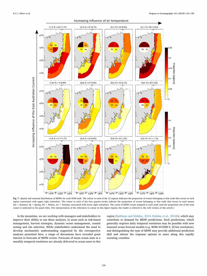
The nodes of the Self Organising Map have also been examined todetermine the regional and seasonal distribution of constituent MHWs(Fig. 7) as well as mean MHW properties (Table 3) and the linear trendin annual MHW days associated with each node (Fig. 8). Each

Table 2Mean state and linear trends in MHW properties for the 12 ETAS regions. Mean values arein units of annual event count (frequency), days (duration, total days), °C (maximumintensity), °C days (cumulative intensity), and m (depth). Trends are in the same units asthe mean, per decade; bold values are statistically significant at the 5% level.

Region Frequency Duration Max. int. Cum. int. Total days Depth

Mean1. EACS 1.52 13.23 1.86 19.0 23.9 1212. EACD 1.87 17.73 1.84 27.7 26.7 1523. CS 1.65 14.75 2.30 26.0 25.4 90.84. CD 1.87 16.30 2.09 28.0 28.5 1625. ZCS 1.61 10.71 2.03 15.4 25.4 93.16. ZCD 1.74 13.84 2.13 23.7 30.3 1857. NEC 1.74 12.19 1.90 17.8 24.8 33.48. OBMP 1.57 12.58 2.23 19.4 22.3 52.59. FHNB 1.83 10.65 2.62 21.2 21.1 28.810. SB 1.74 6.87 2.23 12.1 15.1 21.611. DC 2.00 6.78 2.67 14.8 21.9 22.412. HE 2.00 7.05 2.50 13.3 19.0 27.6

Trend (per decade)1. EACS 1.26 −2.12 −0.323 −4.32 16.8 31.02. EACD 1.72 −5.75 −0.0381 −10.2 22.1 81.63. CS 1.18 −3.48 −0.440 −10.9 13.6 90.14. CD 1.39 −2.65 −0.117 −6.06 21.5 87.65. ZCS 1.05 15.5 −0.209 16.0 35.7 1116. ZCD 1.35 2.50 −0.194 1.72 24.4 60.67. NEC 1.68 −2.00 −0.324 −4.99 22.4 3.688. OBMP 0.988 1.57 −0.519 −0.818 13.2 22.49. FHNB 0.435 3.47 0.00730 5.45 11.8 8.0310. SB 1.95 3.29 0.0488 4.62 21.2 25.611. DC 2.77 5.11 0.0654 10.8 38.0 19.812. HE 2.78 2.73 −0.0500 4.62 30.5 17.5

E.C.J. Oliver et al. Progress in Oceanography 161 (2018) 116–130

120

individual node is characterised in terms of ocean and atmosphericconditions, regional and seasonal distribution, and MHW properties(Appendix A). These descriptions have been qualitatively summarisedin Table 4.

4. Discussion

We first summarise the results relating to the physical oceanogrphy,climate variability and change (Section 4.1) then discuss the ecologicaland management implications (Section 4.2).

Fig. 2. Time series of total MHW days by region. Total annual MHW days are indicated by the black line, the mean by the dashed grey line, and the linear trend by the solid grey line (thetrend is also printed in each panel, including a 95% confidence interval).

Fig. 3. First two EOFs (modes) of variability of total annual MHW days. The (a and c) principal component time series and (b and d) spatial patterns are presented for the first (a and b)and second (c and d) EOFs.

E.C.J. Oliver et al. Progress in Oceanography 161 (2018) 116–130

121

4.1. Physical oceanography, climate variability and change

We have presented the spatial and temporal distribution of marineheatwaves off eastern Tasmania including the mean state and lineartrends, interannual variability, and an event typology. The mean stateindicated a greater frequency and intensity of MHWs in the south of thedomain, but with shorter durations; the opposite pattern is present overthe remainder of the shelf. Linear trends indicated significantly in-creasing frequencies everywere – at a linear rate that doubles the meanstate over a decade. In addition, significant increases in the annualcount of MHW days as well as the penetration depth of MHWs werefound for the nearshore regions off southeastern Tasmania. Strong in-terannual variability in the annual MHW days was evident and could be

primarily decomposed into two modes of variability – the first asso-ciated with year-to-year variations in the East Australian Current andexplaining nearly half of the variability, and the second associated withsemi-persistent ∼5-year variations in a dipole pattern over the shelf.Finally, the hundreds of MHW events spread across the 12 regions ofthe shelf were categorised into 12 types, each with its own set of MHWproperties, regionality, seasonality and associated circulation patterns.Many types were associated with some combination of the EastAustralian Current, offshore anticyclonic eddies, warm air tempera-tures, and/or wind anomalies from northwesterly-to-easterly directions(inclusive clockwise). Notably, event-types were characteristically de-void of cool SSTs over the shelf, northward ocean currents, or windanomalies from westerly or southerly directions.

Fig. 4. Regional ocean and atmospheric circulation and temperature associated with the two modes of interannual variability. Presented are anomalies of sea surface temperature(colours, left), surface currents (arrows, left), air temperature (colours, right) and surface winds (arrows, right) after projection onto the (upper) first and (lower) second EOF modes oftotal annual MHW days. The two reference bars (over land) indicate (upper) an ocean current of 0.05m s−1 and (lower) a wind speed of 0.2 m s−1. (For interpretation of the references tocolour in this figure legend, the reader is referred to the web version of this article.)

E.C.J. Oliver et al. Progress in Oceanography 161 (2018) 116–130

122

These results have implications for understanding climate change inthe region and the predictability of extreme ocean temperatures. Thatthe southeastern part of Tasmania is a region of strong positive trends inmarine heatwave properties is consistent with our understanding of thisregion as a front line of climate change. The east coast of Tasmania isthe climatological boundary between the East Australian Current (EAC)and the Zeehan Current (ZC; Oliver et al., 2016), with the EAC being

substantially warmer than the ZC and penetrating further south due toanthropogenic climate change (Ridgway, 2007; Oliver and Holbrook,2014). Therefore, as the boundary between the two currents pushessouth, regions formerly unexposed to the warm waters of the EAC willpresent a strong and significant response expressed through meanwarming and increases in extremes – with likely ecological impacts.Associated with this long term warming are predictable interannual

Fig. 5. Average ocean states during each of the 12 Self Organising Map (SOM) nodes. Colours (arrows) indicate SSTs (surface current) anomalies averaged across all events assigned tothat node. The count of MHW events assigned to each node (and the proportion out of the total count) is indicated in the panel titles. The reference bar (over land) indicates an oceancurrent of 0.15m s−1. (For interpretation of the references to colour in this figure legend, the reader is referred to the web version of this article.)

E.C.J. Oliver et al. Progress in Oceanography 161 (2018) 116–130

123

variations in MHWs. As our analysis shows, large-scale year-to-yearpulses of the potentially predictable EAC lead to interannual variationsin the count of annual MHWs and these are superimposed on persistentmulti-year variations. Finally, the set of 12MHW types offer a form of“synoptic typing” in that they are associated with large-scale oceanicand atmospheric circulation patterns. If these patterns are present (orforecast) then the region may be predisposed to the occurrence ofMHWs of the types described here. For example, if strong EAC

conditions and northeasterly wind anomalies are forecast (using ex-isting coarse-resolution forecast systems) during the Spring or Summerwe might expect an increased likelihood of short and intense MHWevents across the whole region (i.e. node (4,1) – see Table 4), withouthaving to explicitly forecast the coastal ocean itself at high-resolution.In contrast, the absence of these patterns indicates a predisposition for alack of such MHWs in the region.

Fig. 6. Average atmospheric states during each of the 12 Self Organising Map (SOM) nodes. Colours (arrows) indicate surface air temperatures (surface wind) anomalies averaged acrossall events assigned to that node. The count of MHW events assigned to each node (and the proportion out of the total count) is indicated in the panel titles. The reference bar (over land)indicates a wind speed of 3m s−1. (For interpretation of the references to colour in this figure legend, the reader is referred to the web version of this article.)

E.C.J. Oliver et al. Progress in Oceanography 161 (2018) 116–130

124

4.2. Ecological and management implications

Ecological impacts associated with these MHWs can be revealed byshort and long-term scientific studies, industry records, and citizenscience observations. This historical MHW analysis for easternTasmania aims to shed light on previous ecological impacts for a rangeof researchers and marine users.

Rapid changes and tipping points may occur as a result of extremeevents (Plagányi et al., 2014). In other regions, single MHWs have re-sulted in fish kills (e.g. Wernberg et al., 2013) and dramatic habitatchanges (e.g. Wernberg et al., 2016; Hughes et al., 2017) that will likelypersist for some time. Although there have been some climate-relatedlong-term ecological changes in this study region (see Section 1), dra-matic MHW impacts in this natural environment have been limited,although acute stress on aquaculture species does occur (Hobday et al.,2016b; Oliver et al., 2017a). The southerly location of Tasmania re-lative to the Australasian continent means that coastal species foundhere are likely to be living in the cooler end of the thermal preferencespectrum (e.g. Stuart-Smith et al., 2015), and so even summer MHWchanges in temperature have not exceeded critical temperaturethresholds for the majority of local species (Oliver et al., 2017a).Conversely, milder winters due to climate-related warming, inter-spersed with MHWs, facilitate southward range expansion of species toTasmania (e.g. sea urchin, Centrostephanus rodgersii, Ling et al., 2008;Ling et al., 2009b; numerous fish, Last et al., 2010; Robinson et al.,2015). For example, the establishment and gradual build-up of Cen-trostephanus rodgersii within Tasmanian kelp beds can lead to an eco-logical tipping-point (Ling et al., 2009a, 2015), which is reinforced bydirect loss of kelps due to dieback during extreme conditions (e.g.Valentine and Johnson, 2003; Johnson et al., 2011; S. Ling, pers. obs.).In the present study, significant positive trends were found for MHWtypes (2,3) and (3,3) – winter MHWs which could be of importance forsea urchin larval development for larvae spawned in Tasmanian waters– and for type (4,1) – spring/summer MHWs associated with an EACinfluence and conditions whereby greatest influx of Centrostephanuslarvae from mainland Australia may occur.

There is also the potential for MHWs to impact the occurrence ofviruses and harmful algal blooms, of great importance to the fisheriesand aquaculture industries in Tasmania. For example, the 2015/16MHW in the Tasman Sea led to an outbreak of Pacific Oyster MortalitySyndrome, a virus linked to warmer waters (Green et al., 2014), withsignificant impact on the oyster industry (Oliver et al., 2017a). On the

other hand, the response of harmful algal blooms appears to be stronglydependent on water column stratification (Hallegraeff, 2010), whichcan be influenced by MHWs. The response of harmful algal blooms isfurther dependent on the seasonal timing of MHWs: i.e. along easternTasmania, warming at the end of the cool season (October-November)driving water temperatures above 15 °C could terminate blooms earlier,while conversely an earlier event (May-June) could enhance the growthseason (Gustaaf Hallegraef, IMAS, pers. comm.). For example, a recentmarine heatwave (Spring/Summer of 2017) in the Tasman Sea andsouth of Tasmania briefly touched the east coast of Tasmania, where itended a paralytic shellfish poisoning bloom, allowing for the opening ofthe lobster fishery (Alistair Hobday, CSIRO, pers. comm.).

A workshop describing these Tasmanian MHW results was held inMarch 2017 with managers and marine resource users representingwild fisheries (lobster, abalone, finfish), and coastal aquaculture busi-nesses (salmon, mussel, oyster). These and subsequent discussions re-vealed that managers still see MHW events largely as “natural” al-though the perception of being climate-related is increasing due to thegeneral warming trend off eastern Tasmania (Holbrook and Bindoff,1997; Ridgway, 2007), and commentary around eastern TasmaniaMHW events in 2012 (Hodgkinson et al., 2014) and 2015 (Oliver et al.,2017a) where impacts on farmed species were reported. An increasedscientific ability to do attribution studies also provides new climate-related evidence to marine stakeholders (e.g. Oliver et al., 2017a).

Importantly in this region, long term ocean warming trends andassociated impacts are understood by recreational fishers (van Puttenet al., 2014), commercial fishers (Nursey-Bray et al., 2012; Pecl et al.,2014) and aquaculture businesses (Spillman and Hobday, 2014), due tothe pervasive nature of the long-term changes in distribution, abun-dance, and phenology already observed (Johnson et al., 2011; Frusheret al., 2014). The connection with the poleward-flowing East AustralianCurrent for both long-term warming (Ridgway, 2007) and extremes(Oliver et al., 2014, 2017a; this paper) means that environmental un-derstanding that stakeholders have based on long-term trends can beextended to include extremes such as MHWs, such as was recognised forthe 2011 Western Australia marine heatwave (Metcalf et al., 2015).This positions regional fishery and aquaculture managers to use thesehistorical data to understand past impacts as well as prepare for futurerisks. For example, aquaculture managers, with their greater systemcontrol, can implement a range of responses during MHW events, andthe typological classification may help refine these choices (Spillmanand Hobday, 2014). Cooler areas can be identified for different MHWtypes and some activities relocated to these areas, stocking densities canbe reduced, and harvesting can be initiated earlier. Fishery and en-vironmental managers with whom we discussed this work had a par-ticular interest in the subsequent effects of MHW events such as delayedmortality, reduced recruitment or breeding success. These marinemanagers indicated that although they have few responses that they canapply during a MHW, they may make adjustments in subsequent years,for example, to harvesting levels, if effects persist at longer time scales.While the overwhelming focus of climate change related temperatureeffects is mortality of sensitive taxa, sub-lethal physiological stressleading to reproductive failure may have far greater consequences forpopulation dynamics through recruitment failure. The typology ofMHWs, when combined with retrospective analysis of ecological im-pacts might allow estimation of the subsequent ecological impacts fordifferent MHW types, and thus inform management responses. Un-certainty about the relative effect of MHW duration and intensity oncoastal ecological systems, and thus on the resources that stakeholdersfarm or harvest, necessitates additional study in partnership with theseindustries.

Table 3Average MHW properties for each SOM node. The Frequency columns shows the totalnumber of MHW events in each node, and in brackets the percentage from the total of 486events. The remaining columns show the MHW durations (days), maximum intensities(°C), cumulative (°C days) and depths (m) averaged across all events in each node.

Node Frequency Duration Max. int. Cum. int. Depth

(1,1) 54 (11.1%) 18.4 1.84 26.2 113(2,1) 47 (9.7%) 14.7 2.25 24.0 127(3,1) 48 (9.9%) 10.5 2.29 19.8 85.4(4,1) 69 (14.2%) 7.5 2.46 15.3 98.9(1,2) 14 (2.9%) 25.0 2.07 36.2 102(2,2) 27 (5.6%) 17.1 2.21 29.4 86.3(3,2) 10 (2.1%) 14.8 2.27 26.4 112(4,2) 35 (7.2%) 10.5 2.39 20.7 111(1,3) 57 (11.7%) 14.9 1.63 19.9 128(2,3) 33 (6.8%) 18.2 1.80 22.9 114(3,3) 35 (7.2%) 16.3 1.92 23.3 60.4(4,3) 57 (11.7%) 8.5 1.94 13.5 82.0

E.C.J. Oliver et al. Progress in Oceanography 161 (2018) 116–130

125

In the meantime, we are working with managers and stakeholders toimprove their ability to use these analyses, in areas such as risk-basedmanagement, harvest strategies, dynamic ocean management, coastalzoning and site selection. While stakeholders understand the need todevelop mechanistic understanding supported by the retrospectiveanalyses presented here, a range of discussions have revealed greatinterest in forecasts of MHW events. Forecasts of mean ocean state at amonthly temporal resolution are already delivered to ocean users in this

region (Spillman and Hobday, 2014; Hobday et al., 2016b), which maycontribute to demand for MHW predictions. Such predictions, whichgenerally requires daily temporal resolution may be possible with newseasonal ocean forecast models (e.g. BOM ACCESS S, 25 km resolution),and distinguishing the type of MHW may provide additional predictionskill and inform the response options to users along this rapidlywarming coastline.

Fig. 7. Spatial and seasonal distribution of MHWs for each SOM node. The colour in each of the 12 regions indicates the proportion of events belonging to that node that occurs in eachregion (associated with upper right colourbar). The colour in each of the four quarter-circles indicate the proportion of events belonging to that node that occurs in each season(Su= Summer, Sp= Spring, Wi=Winter, Au=Autumn; associated with lower right colourbar). The count of MHW events assigned to each node (and the proportion out of the totalcount) is indicated in the panel titles. (For interpretation of the references to colour in this figure legend, the reader is referred to the web version of this article.)

E.C.J. Oliver et al. Progress in Oceanography 161 (2018) 116–130

126

Acknowledgements

This work was funded by a University of Tasmania (UTAS) ResearchEnhancement Granting Scheme (REGS) 2016 grant (Oliver, Holbrook,Ling, Mundy and Hobday, 2016, Identifying historical marine heatwavesoff eastern Tasmania, UTAS REGS 2016, Grant No. O0023890). ECJOacknowledges funding from the Australian Research Council Centre ofExcellence for Climate System Science (Grant No. CE110001028). NJHacknowledges funding from the Australian Research Council Centre ofExcellence for Climate Extremes (Grant No. CE170100023). This papermakes a contribution to NESP Earth Systems Science and ClimateChange Hub Project 2.3 (component 2) on the predictability of oceantemperature extremes. The ecological and management implicationswere partly informed by the “Marine Heatwaves StakeholderWorkshop: Marine heatwaves off eastern Tasmania: trends, variability,and typologies” held at the University of Tasmania on 20 March 2017,bringing together representatives from science (oceanographers, ecol-ogists), industry (fisheries, aquculture), and Tasmanian state

government departments. The ETAS ocean model data is availablethrough the IMAS data portal (data.imas.utas.edu.au). The Bluelinkocean data products were provided by CSIRO; Bluelink is a collabora-tion involving the Commonwealth Bureau of Meteorology, theCommonwealth Scientific and Industrial Research Organisation and theRoyal Australian Navy. The National Centers for EnvironmentalPrediction (NCEP) Climate Forecast System (CFS) Reanalysis andVersion 2 analysis data were provided by the Research Data Archive atthe National Center for Atmospheric Research, Computational andInformation Systems Laboratory.

Appendix A. Description of the MHW types

Below are descriptions of each of the 12 MHW types (SOM nodes).

A.1. Node (1,1)

Node (1,1) exhibits broad southward flow both on and off the shelf,

Fig. 8. Annual time series of MHW days associated with each SOM node. Panels with red bars indicate a statistically significant ( <p 0.05) linear trend. The count of MHW events assignedto each node (and the proportion out of the total count) is indicated in the panel titles.

Table 4Qualitative summary of the MHW typology. The regions commonly represented, seasonal occurrence, MHW properties, and associated ocean and atmospheric conditions are presentedfor each SOM node. The following definitions were used for the descriptive terms: frequent meant ⩾10%, infrequent meant ⩽5%, long (short) events lasted at least (most) 18 (10) days,intense (weak) events had a maximum intensity of at least (most) 2.2 °C (1.8 °C), deep events extended vertically over at least 110m, the only node marked shallow had the shallowestevents of all nodes. Acronyms are defined as: SE=Southeast, N=North, E=East, NE=Northeast, NW=Northwest, EAC=East Australian Current, AC=Anticyclonic. Region namesare defined in Fig. 1.

Node Region Season MHW properties Conditions

(1,1) All Autumn Frequent, long, deep Broad southward flow on and off the shelf, E-erly winds(2,1) All exc. SE coastal and NE offshore Spring Intense, deep EAC flow over shelf, AC eddy off the SE, E-erly winds(3,1) All Spring, Summer Intense, fast onset and decline EAC flow over shelf, AC eddy off the SE, NE-erly winds(4,1) All Spring, Summer Frequent, intense, short, fast onset Strong EAC, large spatial scale, warm air, N-erly winds(1,2) ZCD, CD Summer Infrequent, long EAC flow over shelf(2,2) ZCS, HE Summer Intense, fast decline Broad southward flow over shelf, eddy off the SE(3,2) OBMP All Infrequent, intense, deep Eddy train offshore(4,2) OBMP, northern, eastern offshore Spring, Summer Intense, deep Eddy train offshore, warm air, N-erly winds(1,3) Northeast Autumn, Winter Frequent, weak, deep, slow onset and decline Weak flow over shelf, eddy train offshore, weak atmosphere(2,3) EACD, OBMP, FHNB, DC Winter Weak, long, deep Weak flow over shelf(3,3) Southeast coastal and OBMP Winter Shallow Eddy off the SE, moderate strength Zeehan Current(4,3) Southeast coastal and ZCD Autumn, Winter Frequent, short, shallow Strong Zeehan Current, warm air, NW-erly winds

E.C.J. Oliver et al. Progress in Oceanography 161 (2018) 116–130

127

a hotspot of warm SSTAs (∼1 °C) centred on the shelf between theFreycinet and Tasman Peninsulas, strong easterly winds and relativelylow air temperature anomalies (⩽1 °C). This node occurs frequently(11.1% of all events) and MHWs are distributed across all regions, al-through perhaps more in the south than north. Events occurred pre-dominantly in the Autumn and on average were long (18.4 days) anddeep (113m). Annual marine heatwave days associated with this nodehad a statistically significant linear increase of 8.95 days decade−1.

A.2. Node (2,1)

Node (2,1) exhibits broad southward flow both on and off the shelf(with offshore flow indicating an influence of the EAC), an anticycloniceddy off southeastern Tasmania, warm SSTAs (up to ∼2 °C) over themost of the shelf (but stronger in the south), moderate easterly windanomalies and moderate air temperature anomalies 1–2.5 °C). Thisnode occurs relatively frequently (9.9% of all events) and MHWs aredistributed across most regions, excluding EACD and the nearshoreregions of the southeast. Events occurred predominantly in the Springand on average were intense (2.25 °C) and deep (127m). Annualmarine heatwave days associated with this node had a statisticallysignificant linear increase of 8.56 days decade−1.

A.3. Node (3,1)

Node (3,1) exhibits broad southward flow both on and off the shelf(with offshore flow indicating an influence of the EAC), an anticycloniceddy off southeastern Tasmania, warm SSTAs (up to ∼2 °C) over thecentral and offshore southern parts of the shelf, strong northeasterlywind anomalies and moderate air temperature anomalies over the shelf(1–2 °C). This node occurs relatively frequently (9.7% of all events) andMHWs are distributed across most regions, excluding EACD and thenearshore regions of the southeast. Events occurred predominantly inthe Spring and Summer and on average were intense (2.29 °C) with fastonset and decline rates (onset and decline rates not shown, see Oliveret al. (2017b) details).

A.4. Node (4,1)

Node (4,1) exhibits strong southward flow both on and off the shelf(with a strong signature of the EAC offshore), very warm SSTAs (up to∼3 °C) over the entire shelf, strong northeasterly wind anomalies andwarm air temperature anomalies over the shelf (2–4 °C). This nodeoccurs the most frequently of all nodes (14.2% of all events) and MHWsare distributed across all regions. Events occurred only in the Springand Summer and on average were the most intense (2.46 °C) andshortest (7.5 days) of all nodes, with fast onset rates. Annual marineheatwave days associated with this node had a statistically significantlinear increase of 5.12 days decade−1.

A.5. Node (1,2)

Node (1,2) exhibits broad southward flow both on and off the shelf,warm SSTAs (∼1 °C) predominantly away from the coast off the southof the shelf, moderate easterly wind anomalies and relatively low airtemperature anomalies (∼1 °C). This node occurs infrequently (2.9% ofall events) and MHWs are distributed primarily in the offshore south-east (CD, ZCD) regions. Events occurred predominantly in the Summerand on average were the longest of all nodes (25.0 days).

A.6. Node (2,2)

Node (2,2) exhibits southward flow over the shelf, an anticycloniceddy off southeastern Tasmania, warm SSTAs (∼1 °C) over most of theshelf, moderate northeasterly wind anomalies and moderate air tem-perature anomalies (1–2.5 °C). In this node occurs 5.6% of all eventsand MHWs are distributed primarily in the ZCS and HE regions. Eventsoccurred predominantly in the Summer and on average were intense(2.21 °C) with fast decline rates.

A.7. Node (3,2)

Node (3,2) exhibits a train of eddies running parallel to (and justoffshore) the shelf edge, warm SSTAs (up to ∼2 °C) over most of thesouthern half of the shelf, moderate northerly wind anomalies andmoderate air temperature anomalies (1–2 °C). This node occurs themost infrequently (2.1% of all events) and most MHWs were in theOBMP region. Events occurred across all seasons (with a slight pre-ference for Spring and Summer) and on average were intense (2.27 °C)and deep (112m).

A.8. Node (4,2)

Node (4,2) exhibits a train of eddies running parallel to (and justoffshore) the shelf edge, very warm SSTAs (up to 1–2.5 °C) over most ofthe shelf, stong northerly wind anomalies and warm air temperatureanomalies (2–3 °C). In this node occurs 7.2% of all events and mostMHWs were in the OBMP region, with some across the northern regionsand offshore to the east. Events occurred predominantly in the Springand Summer and on average were intense (2.39 °C) and deep (111m)

A.9. Node (1,3)

Node (1,3) exhibits weak flow over the shelf, a train of eddiesrunning parallel to (and just offshore) the shelf edge, SSTAs of ⩽1 °Cincreasing to the north, very weak wind anomalies and very low airtemperature anomalies (⩽1 °C). This node occurs frequently (11.7% ofall events) and MHWs are distributed primarily in the northern regions.Events occurred predominantly in the Winter and Autumn and onaverage were the weakest (1.63 °C) but deepest (128m) of all nodes,with slow onset and decline rates.

A.10. Node (2,3)

Node (2,3) exhibits weak flow over the shelf, SSTAs of ⩽1 °C overthe shelf except in the coastal southeastern regions where SSTAs wereup to 2 °C, moderate northerly wind anomalies and moderate air tem-perature anomalies (1–2 °C). In this node occurs 6.8% of all events andMHWs are distributed across the shelf with little spatial structure(highest numbers in EACD, OBMP, FHNB and DC). Events occurredpredominantly in the Winter and on average were weak (1.80 °C), long(18.2 days) and deep (114m). Annual marine heatwave days associatedwith this node had a statistically significant linear increase of 21.7 daysdecade−1.

A.11. Node (3,3)

Node (3,3) exhibits weak flow over most of the shelf except for amoderate strength Zeehan Current flowing eastward over the southernportion, an anticyclonic eddy off southeastern Tasmania, SSTAs of⩽1 °C over the shelf except in the coastal southeastern regions whereSSTAs were up to 2 °C, moderate-to-strong northerly wind anomalies

E.C.J. Oliver et al. Progress in Oceanography 161 (2018) 116–130

128

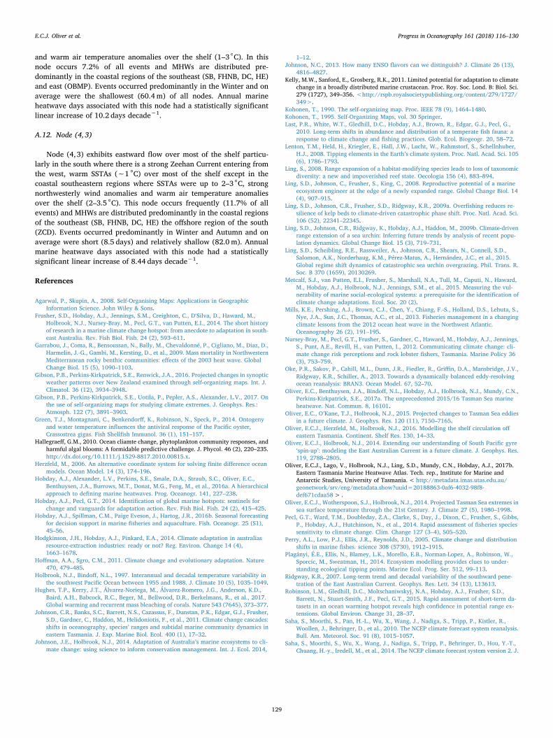
and warm air temperature anomalies over the shelf (1–3 °C). In thisnode occurs 7.2% of all events and MHWs are distributed pre-dominantly in the coastal regions of the southeast (SB, FHNB, DC, HE)and east (OBMP). Events occurred predominantly in the Winter and onaverage were the shallowest (60.4m) of all nodes. Annual marineheatwave days associated with this node had a statistically significantlinear increase of 10.2 days decade−1.

A.12. Node (4,3)

Node (4,3) exhibits eastward flow over most of the shelf particu-larly in the south where there is a strong Zeehan Current entering fromthe west, warm SSTAs (∼1 °C) over most of the shelf except in thecoastal southeastern regions where SSTAs were up to 2–3 °C, strongnorthwesterly wind anomalies and warm air temperature anomaliesover the shelf (2–3.5 °C). This node occurs frequently (11.7% of allevents) and MHWs are distributed predominantly in the coastal regionsof the southeast (SB, FHNB, DC, HE) the offshore region of the south(ZCD). Events occurred predominantly in Winter and Autumn and onaverage were short (8.5 days) and relatively shallow (82.0 m). Annualmarine heatwave days associated with this node had a statisticallysignificant linear increase of 8.44 days decade−1.

References

Agarwal, P., Skupin, A., 2008. Self-Organising Maps: Applications in GeographicInformation Science. John Wiley & Sons.

Frusher, S.D., Hobday, A.J., Jennings, S.M., Creighton, C., D‘Silva, D., Haward, M.,Holbrook, N.J., Nursey-Bray, M., Pecl, G.T., van Putten, E.I., 2014. The short historyof research in a marine climate change hotspot: from anecdote to adaptation in south-east Australia. Rev. Fish Biol. Fish. 24 (2), 593–611.

Garrabou, J., Coma, R., Bensoussan, N., Bally, M., Chevaldonné, P., Cigliano, M., Diaz, D.,Harmelin, J.-G., Gambi, M., Kersting, D., et al., 2009. Mass mortality in NorthwesternMediterranean rocky benthic communities: effects of the 2003 heat wave. GlobalChange Biol. 15 (5), 1090–1103.

Gibson, P.B., Perkins-Kirkpatrick, S.E., Renwick, J.A., 2016. Projected changes in synopticweather patterns over New Zealand examined through self-organizing maps. Int. J.Climatol. 36 (12), 3934–3948.

Gibson, P.B., Perkins-Kirkpatrick, S.E., Uotila, P., Pepler, A.S., Alexander, L.V., 2017. Onthe use of self-organizing maps for studying climate extremes. J. Geophys. Res.:Atmosph. 122 (7), 3891–3903.

Green, T.J., Montagnani, C., Benkendorff, K., Robinson, N., Speck, P., 2014. Ontogenyand water temperature influences the antiviral response of the Pacific oyster,Crassostrea gigas. Fish Shellfish Immunol. 36 (1), 151–157.

Hallegraeff, G.M., 2010. Ocean cliamte change, phytoplankton community responses, andharmful algal blooms: A formidable predictive challenge. J. Phycol. 46 (2), 220–235.http://dx.doi.org/10.1111/j.1529-8817.2010.00815.x.

Herzfeld, M., 2006. An alternative coordinate system for solving finite difference oceanmodels. Ocean Model. 14 (3), 174–196.

Hobday, A.J., Alexander, L.V., Perkins, S.E., Smale, D.A., Straub, S.C., Oliver, E.C.,Benthuysen, J.A., Burrows, M.T., Donat, M.G., Feng, M., et al., 2016a. A hierarchicalapproach to defining marine heatwaves. Prog. Oceanogr. 141, 227–238.

Hobday, A.J., Pecl, G.T., 2014. Identification of global marine hotspots: sentinels forchange and vanguards for adaptation action. Rev. Fish Biol. Fish. 24 (2), 415–425.

Hobday, A.J., Spillman, C.M., Paige Eveson, J., Hartog, J.R., 2016b. Seasonal forecastingfor decision support in marine fisheries and aquaculture. Fish. Oceanogr. 25 (S1),45–56.

Hodgkinson, J.H., Hobday, A.J., Pinkard, E.A., 2014. Climate adaptation in australiasresource-extraction industries: ready or not? Reg. Environ. Change 14 (4),1663–1678.

Hoffman, A.A., Sgro, C.M., 2011. Climate change and evolutionary adaptation. Nature470, 479–485.

Holbrook, N.J., Bindoff, N.L., 1997. Interannual and decadal temperature variability inthe southwest Pacific Ocean between 1955 and 1988. J. Climate 10 (5), 1035–1049.

Hughes, T.P., Kerry, J.T., Álvarez-Noriega, M., Álvarez-Romero, J.G., Anderson, K.D.,Baird, A.H., Babcock, R.C., Beger, M., Bellwood, D.R., Berkelmans, R., et al., 2017.Global warming and recurrent mass bleaching of corals. Nature 543 (7645), 373–377.

Johnson, C.R., Banks, S.C., Barrett, N.S., Cazassus, F., Dunstan, P.K., Edgar, G.J., Frusher,S.D., Gardner, C., Haddon, M., Helidoniotis, F., et al., 2011. Climate change cascades:shifts in oceanography, species’ ranges and subtidal marine community dynamics ineastern Tasmania. J. Exp. Marine Biol. Ecol. 400 (1), 17–32.

Johnson, J.E., Holbrook, N.J., 2014. Adaptation of Australia’s marine ecosystems to cli-mate change: using science to inform conservation management. Int. J. Ecol. 2014,

1–12.Johnson, N.C., 2013. How many ENSO flavors can we distinguish? J. Climate 26 (13),

4816–4827.Kelly, M.W., Sanford, E., Grosberg, R.K., 2011. Limited potential for adaptation to climate

change in a broadly distributed marine crustacean. Proc. Roy. Soc. Lond. B: Biol. Sci.279 (1727), 349–356. <http://rspb.royalsocietypublishing.org/content/279/1727/349>.

Kohonen, T., 1990. The self-organizing map. Proc. IEEE 78 (9), 1464–1480.Kohonen, T., 1995. Self-Organizing Maps, vol. 30 Springer.Last, P.R., White, W.T., Gledhill, D.C., Hobday, A.J., Brown, R., Edgar, G.J., Pecl, G.,

2010. Long-term shifts in abundance and distribution of a temperate fish fauna: aresponse to climate change and fishing practices. Glob. Ecol. Biogeogr. 20, 58–72.

Lenton, T.M., Held, H., Kriegler, E., Hall, J.W., Lucht, W., Rahmstorf, S., Schellnhuber,H.J., 2008. Tipping elements in the Earth’s climate system. Proc. Natl. Acad. Sci. 105(6), 1786–1793.

Ling, S., 2008. Range expansion of a habitat-modifying species leads to loss of taxonomicdiversity: a new and impoverished reef state. Oecologia 156 (4), 883–894.

Ling, S.D., Johnson, C., Frusher, S., King, C., 2008. Reproductive potential of a marineecosystem engineer at the edge of a newly expanded range. Global Change Biol. 14(4), 907–915.

Ling, S.D., Johnson, C.R., Frusher, S.D., Ridgway, K.R., 2009a. Overfishing reduces re-silience of kelp beds to climate-driven catastrophic phase shift. Proc. Natl. Acad. Sci.106 (52), 22341–22345.

Ling, S.D., Johnson, C.R., Ridgway, K., Hobday, A.J., Haddon, M., 2009b. Climate-drivenrange extension of a sea urchin: Inferring future trends by analysis of recent popu-lation dynamics. Global Change Biol. 15 (3), 719–731.

Ling, S.D., Scheibling, R.E., Rassweiler, A., Johnson, C.R., Shears, N., Connell, S.D.,Salomon, A.K., Norderhaug, K.M., Pérez-Matus, A., Hernández, J.C., et al., 2015.Global regime shift dynamics of catastrophic sea urchin overgrazing. Phil. Trans. R.Soc. B 370 (1659), 20130269.

Metcalf, S.J., van Putten, E.I., Frusher, S., Marshall, N.A., Tull, M., Caputi, N., Haward,M., Hobday, A.J., Holbrook, N.J., Jennings, S.M., et al., 2015. Measuring the vul-nerability of marine social-ecological systems: a prerequisite for the identification ofclimate change adaptations. Ecol. Soc. 20 (2).

Mills, K.E., Pershing, A.J., Brown, C.J., Chen, Y., Chiang, F.-S., Holland, D.S., Lehuta, S.,Nye, J.A., Sun, J.C., Thomas, A.C., et al., 2013. Fisheries management in a changingclimate lessons from the 2012 ocean heat wave in the Northwest Atlantic.Oceanography 26 (2), 191–195.

Nursey-Bray, M., Pecl, G.T., Frusher, S., Gardner, C., Haward, M., Hobday, A.J., Jennings,S., Punt, A.E., Revill, H., van Putten, I., 2012. Communicating climate change: cli-mate change risk perceptions and rock lobster fishers, Tasmania. Marine Policy 36(3), 753–759.

Oke, P.R., Sakov, P., Cahill, M.L., Dunn, J.R., Fiedler, R., Griffin, D.A., Mansbridge, J.V.,Ridgway, K.R., Schiller, A., 2013. Towards a dynamically balanced eddy-resolvingocean reanalysis: BRAN3. Ocean Model. 67, 52–70.

Oliver, E.C., Benthuysen, J.A., Bindoff, N.L., Hobday, A.J., Holbrook, N.J., Mundy, C.N.,Perkins-Kirkpatrick, S.E., 2017a. The unprecedented 2015/16 Tasman Sea marineheatwave. Nat. Commun. 8, 16101.

Oliver, E.C., O’Kane, T.J., Holbrook, N.J., 2015. Projected changes to Tasman Sea eddiesin a future climate. J. Geophys. Res. 120 (11), 7150–7165.

Oliver, E.C.J., Herzfeld, M., Holbrook, N.J., 2016. Modelling the shelf circulation offeastern Tasmania. Continent. Shelf Res. 130, 14–33.

Oliver, E.C.J., Holbrook, N.J., 2014. Extending our understanding of South Pacific gyre‘spin-up’: modeling the East Australian Current in a future climate. J. Geophys. Res.119, 2788–2805.

Oliver, E.C.J., Lago, V., Holbrook, N.J., Ling, S.D., Mundy, C.N., Hobday, A.J., 2017b.Eastern Tasmania Marine Heatwave Atlas. Tech. rep., Institute for Marine andAntarctic Studies, University of Tasmania.< http://metadata.imas.utas.edu.au/geonetwork/srv/eng/metadata.show?uuid=20188863-0af6-4032-98f8-def671cdaa58> .

Oliver, E.C.J., Wotherspoon, S.J., Holbrook, N.J., 2014. Projected Tasman Sea extremes insea surface temperature through the 21st Century. J. Climate 27 (5), 1980–1998.

Pecl, G.T., Ward, T.M., Doubleday, Z.A., Clarke, S., Day, J., Dixon, C., Frusher, S., Gibbs,P., Hobday, A.J., Hutchinson, N., et al., 2014. Rapid assessment of fisheries speciessensitivity to climate change. Clim. Change 127 (3–4), 505–520.

Perry, A.L., Low, P.J., Ellis, J.R., Reynolds, J.D., 2005. Climate change and distributionshifts in marine fishes. science 308 (5730), 1912–1915.

Plagányi, É.E., Ellis, N., Blamey, L.K., Morello, E.B., Norman-Lopez, A., Robinson, W.,Sporcic, M., Sweatman, H., 2014. Ecosystem modelling provides clues to under-standing ecological tipping points. Marine Ecol. Prog. Ser. 512, 99–113.

Ridgway, K.R., 2007. Long-term trend and decadal variability of the southward pene-tration of the East Australian Current. Geophys. Res. Lett. 34 (13), L13613.

Robinson, L.M., Gledhill, D.C., Moltschaniwskyj, N.A., Hobday, A.J., Frusher, S.D.,Barrett, N., Stuart-Smith, J.F., Pecl, G.T., 2015. Rapid assessment of short-term da-tasets in an ocean warming hotspot reveals high confidence in potential range ex-tensions. Global Environ. Change 31, 28–37.

Saha, S., Moorthi, S., Pan, H.-L., Wu, X., Wang, J., Nadiga, S., Tripp, P., Kistler, R.,Woollen, J., Behringer, D., et al., 2010. The NCEP climate forecast system reanalysis.Bull. Am. Meteorol. Soc. 91 (8), 1015–1057.

Saha, S., Moorthi, S., Wu, X., Wang, J., Nadiga, S., Tripp, P., Behringer, D., Hou, Y.-T.,Chuang, H.-y., Iredell, M., et al., 2014. The NCEP climate forecast system version 2. J.

E.C.J. Oliver et al. Progress in Oceanography 161 (2018) 116–130

129

Climate 27 (6), 2185–2208.Sanderson, J.C., 1990. M.Sc. Thesis: Subtidal Macroalgal Studies in East and South

Eastern Tasmanian Coastal Waters. University of Tasmania, Hobart, Australia.Schlegel, R.W., Oliver, E.C.J., Perkins-Kirkpatrick, S., Kruger, A., Smit, A.J., 2017.

Predominant atmospheric and oceanic patterns during coastal marine heatwaves.Front. Marine Sci. 4, 323.

Serrao-Neumann, S., Davidson, J.L., Baldwin, C.L., Dedekorkut-Howes, A., Ellison, J.C.,Holbrook, N.J., Howes, M., Jacobson, C., Morgan, E.A., 2016. Marine governance toavoid tipping points: can we adapt the adaptability envelope? Marine Policy 65,56–67.

Sloyan, B.M., O’Kane, T.J., 2015. Drivers of decadal variability in the Tasman Sea. J.Geophys. Res. 120 (5), 3193–3210.

Spillman, C.M., Hobday, A.J., 2014. Dynamical seasonal ocean forecasts to aid salmonfarm management in a climate hotspot. Climate Risk Manage. 1, 25–38.

Stuart-Smith, R.D., Edgar, G.J., Barrett, N.S., Kininmonth, S.J., Bates, A.E., 2015. Thermalbiases and vulnerability to warming in the world’s marine fauna. Nature 528(7580), 88.

Valentine, J.P., Johnson, C.R., 2003. Establishment of the introduced kelp Undaria pin-natifida in Tasmania depends on disturbance to native algal assemblages. J. Exp.Marine Biol. Ecol. 295 (1), 63–90.

Valentine, J.P., Johnson, C.R., 2004. Establishment of the introduced kelp undaria pin-natifida following dieback of the native macroalga Phyllospora comosa in Tasmania,Australia. Marine Freshwater Res. 55 (3), 223–230.

van Putten, I., Metcalf, S., Frusher, S., Marshall, N., Tull, M., 2014. Fishing for the impactsof climate change in the marine sector: a case study. Int. J. Climate Change StrategiesManage. 6 (4), 421–441.

Visser, M.E., 2008. Keeping up with a warming world; assessing the rate of adaptation toclimate change. Proc. Roy. Soc. Lond. B: Biol. Sci. 275 (1635), 649–659. <http://rspb.royalsocietypublishing.org/content/275/1635/649>.

Wernberg, T., Bennett, S., Babcock, R.C., de Bettignies, T., Cure, K., Depczynski, M.,Dufois, F., Fromont, J., Fulton, C.J., Hovey, R.K., et al., 2016. Climate-driven regimeshift of a temperate marine ecosystem. Science 353 (6295), 169–172.

Wernberg, T., Smale, D.A., Tuya, F., Thomsen, M.S., Langlois, T.J., De Bettignies, T.,Bennett, S., Rousseaux, C.S., 2013. An extreme climatic event alters marine eco-system structure in a global biodiversity hotspot. Nat. Climate Change 3 (1), 78–82.

Wilks, D.S., 2006. Statistical Methods in the Atmospheric Sciences. Academic Press.Williams, R.N., de Souza, P.A., Jones, E.M., 2014. Analysing coastal ocean model outputs

using competitive-learning pattern recognition techniques. Environ. Model. Software57, 165–176.

E.C.J. Oliver et al. Progress in Oceanography 161 (2018) 116–130

130

View publication statsView publication stats