Marine and Petroleum Geology - Web hosting

at SciVerse ScienceDirect

Marine and Petroleum Geology xxx (2012) 1e11

Contents lists available

Marine and Petroleum Geology

journal homepage: www.elsevier .com/locate/marpetgeo

Seismic velocities on the Nova Scotian margin to estimate gas hydrate and free gasconcentrations

Angela Schlesinger a,*, Janette Cullen b, George Spence a, Roy Hyndman c, Keith Louden d, David Mosher e

a School of Earth and Ocean Sciences, University of Victoria, Bob Wright Centre, P.O. Box 3065 STN CSC, Victoria, BC V8W 3V6, CanadabDepartment of Earth Sciences, 1459 Oxford Street, Dalhousie University, NS B3H 4R2, Canadac Pacific Geoscience Centre, Geological Survey of Canada, P.O. 6000, Sidney, BC V8L 4B2, CanadadDepartment of Oceanography, Dalhouise University, 1355 Oxford Street, Halifax, NS B3H 4R2, CanadaeGeological Survey of Canada-Atlantic, Bedford Institute of Oceanography, P.O. Box 1006, Dartmouth, NS B2Y 4A2, Canada

a r t i c l e i n f o

Article history:Received 2 September 2011Received in revised form6 February 2012Accepted 20 March 2012Available online xxx

Keywords:Ocean-bottom seismometersWide-angle reflectionsTravel-time tomography2-D velocity modelsNova ScotiaGas hydrate concentrationsFree gas concentrationBSR

* Corresponding author. Tel.: þ1 250 721 6188; faxE-mail address: [email protected] (

0264-8172/$ e see front matter � 2012 Elsevier Ltd.doi:10.1016/j.marpetgeo.2012.03.008

Please cite this article in press as: Schlesingconcentrations, Marine and Petroleum Geol

a b s t r a c t

This article provides new constraints on gas hydrate and free gas concentrations in the sediments at themargin off Nova Scotia. Two-dimensional (2-D) velocity models were constructed through simultaneoustravel-time inversion of ocean-bottom seismometer (OBS) data and 2-D single-channel seismic (SCS)data acquired in two surveys, in 2004 and 2006. The surveys, separated by w5 km, were carried out inregions where the bottom-simulating reflection (BSR) was identified in seismic reflection datasets fromearlier studies and address the question of whether the BSR is a good indicator of significant gas hydrateon the Scotian margin. For both datasets, velocity increases by 200e300 m/s at a depth of approximately220 m below seafloor (mbsf), but the results of the 2006 survey show a smaller velocity decrease (50e80 m/s) at the base of this high-velocity layer (310e330 mbsf) than the results of the 2004 survey(130 m/s). When converted to gas hydrate concentrations using effective medium theory, the 2-Dvelocity models for both datasets show a gas hydrate layer of w100 m thickness above the identifiedBSR. Gas hydrate concentrations are estimated at approximately 2e10% for the 2006 data and 8e18% forthe 2004 survey. The reduction in gas hydrate concentration relative to the distance from the MohicanChannel structure is most likely related to the low porosity within the mud-dominant sediment at thedepth of the BSR. Free gas concentrations were calculated to be 1e2% of the sediment pore space for bothdatasets.

� 2012 Elsevier Ltd. All rights reserved.

1. Introduction

Gas hydrates contain significant amounts of hydrocarbon gas,and so the identification and mapping of gas hydrate occurrencesare important to define a potential massive energy resource.Bottom-simulating reflections (BSR’s), first identified in seismicreflection data at the Blake Ridge (Tucholke et al., 1977), have beenused as an indirect indicator for the presence of gas hydrate andunderlying free gas. Ruppel et al. (2011) conclude that the presenceof a BSR usually indicates that some gas hydrate, most commonly atlow saturation, occurs near the base of the gas hydrate stabilityzone (GHSZ). BSRs are common in the accretionary sedimentaryprisms of active margins but are less common for passive margins.An important question is whether this difference represents muchless hydrate on passive margins or only less prominent BSRs.

: þ1 250 721 6200.A. Schlesinger).

All rights reserved.

er, A., et al., Seismic velocitiogy (2012), doi:10.1016/j.mar

A few areas may host gas hydrate without a visible BSR, such asportions of the Blake Ridge (Holbrook et al., 1996) and the Gulf ofMexico (Dai et al., 2004; GOM 2009). Studies by Xu and Ruppel(1999) show that a missing BSR in a gas hydrate-prone areamight be due to low methane flux into GHSZ. Other possibilitiesinclude local perturbations in temperature, salinity and/ormethaneflux (Ruppel et al., 2011). However, Haacke et al. (2007) argue thatpassive margins without an observable BSR are unlikely to containsignificant quantities of gas hydrate. We therefore have focused onareas with a clear BSR with some data extending to where the BSRis not clear.

The passive margin off eastern Canada was widely mappedduring the past 40 years by the hydrocarbon exploration industry.In 1998/9 the Geological Survey of Canada (GSC) collected a total of34,000 km of two-dimensional (2-D) multi-channel seismic (MCS)data on the Scotian Slope. Therefore, an extensive database ofseismic reflection lines exists for the east coast of Canada. The datawere recently used byMosher (2011) to estimate the distribution ofgas hydrate based on the area where a BSR can be identified

es on the Nova Scotian margin to estimate gas hydrate and free gaspetgeo.2012.03.008

Delta:1_given name

Delta:1_surname

Delta:1_given name

Delta:1_surname

Delta:1_given name

Delta:1_surname

mailto:[email protected]

www.sciencedirect.com/science/journal/02648172

http://www.elsevier.com/locate/marpetgeo

http://dx.doi.org/10.1016/j.marpetgeo.2012.03.008



A. Schlesinger et al. / Marine and Petroleum Geology xxx (2012) 1e112

confidently. However, estimates of gas hydrate concentration arepoorly constrained e no gas hydrate has been recovered on theCanadian Atlantic margin, and there has been limited interpreta-tion of hydrate occurrence based on geophysical downhole logs(Thurber Consultants Ltd.; Neave, 1990) that has not beenconfirmed or calibrated by analysis of recovered hydrate.

Important constraints on gas hydrate concentrations are derivedfrom seismic velocities determined from recordings of wide-anglereflections and refractions on ocean-bottom seismometers (OBS)and long-offset MCS streamer systems. Recent one-dimensional (1-D) velocity-depth profiles were obtained from waveform tomog-raphy on a 45 km long MCS profile (Delescluse et al., 2011). Mosher(2011) reported velocity results from four OBS surveys on theAtlantic margin, based on 1-D interpretations of individual OBSs.However, in only one survey (LeBlanc et al., 2007) were seismicvelocities converted to gas hydrate and free gas concentrations,using an effective medium model (Dvorkin et al., 1999) to obtainestimates of 2e6% bulk gas hydrate and less than 1% free gas in thepore space.

In this paper, we provide improved constraints on gas hydrateand free gas concentrations and volumes on the Atlantic margin ofCanada, through careful determination of seismic velocities in theregion of the Mohican Channel (Fig. 1) where a prominent BSR wasidentified. For two surveys, in 2004 and 2006, we constructed 2-Dmodels of velocity through simultaneous inversion of travel-timesfrom arrays of OBSs and from 2-D single-channel seismic (SCS)profiles.

2. Seismic data acquisition and processing

2.1. Ocean-bottom seismometer and single-channel seismic data

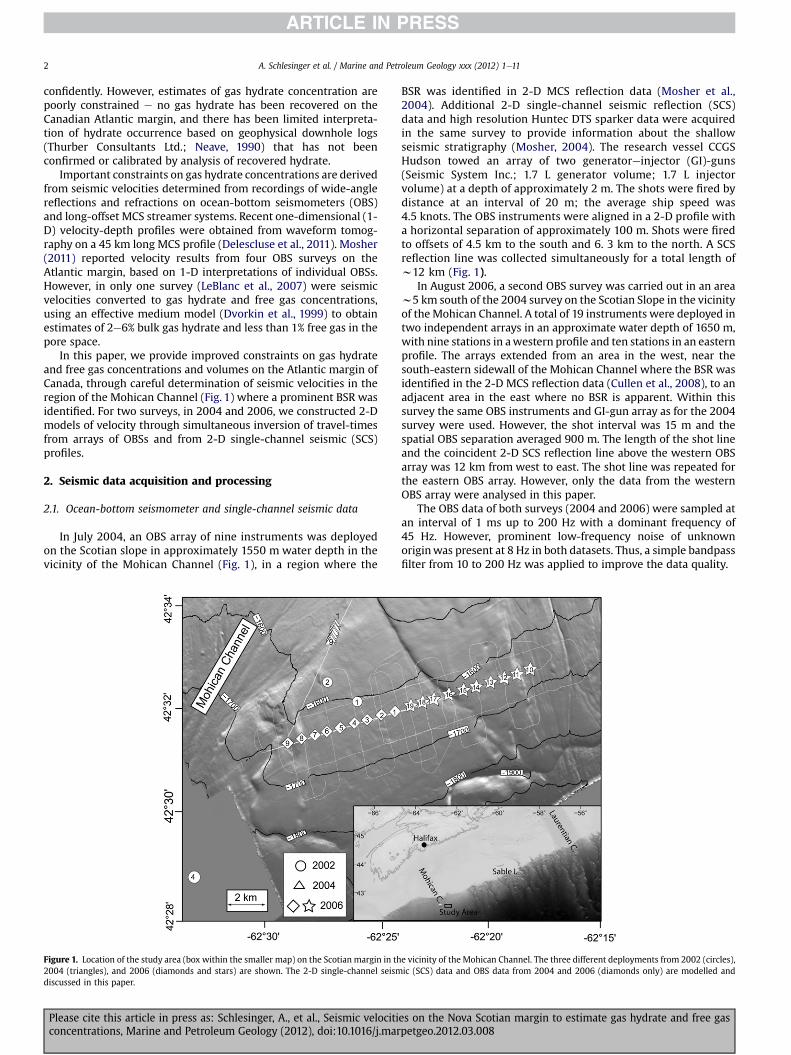
In July 2004, an OBS array of nine instruments was deployedon the Scotian slope in approximately 1550 m water depth in thevicinity of the Mohican Channel (Fig. 1), in a region where the

Figure 1. Location of the study area (box within the smaller map) on the Scotian margin in th2004 (triangles), and 2006 (diamonds and stars) are shown. The 2-D single-channel seismdiscussed in this paper.

Please cite this article in press as: Schlesinger, A., et al., Seismic velociticoncentrations, Marine and Petroleum Geology (2012), doi:10.1016/j.mar

BSR was identified in 2-D MCS reflection data (Mosher et al.,2004). Additional 2-D single-channel seismic reflection (SCS)data and high resolution Huntec DTS sparker data were acquiredin the same survey to provide information about the shallowseismic stratigraphy (Mosher, 2004). The research vessel CCGSHudson towed an array of two generatoreinjector (GI)-guns(Seismic System Inc.; 1.7 L generator volume; 1.7 L injectorvolume) at a depth of approximately 2 m. The shots were fired bydistance at an interval of 20 m; the average ship speed was4.5 knots. The OBS instruments were aligned in a 2-D profile witha horizontal separation of approximately 100 m. Shots were firedto offsets of 4.5 km to the south and 6. 3 km to the north. A SCSreflection line was collected simultaneously for a total length ofw12 km (Fig. 1).

In August 2006, a second OBS survey was carried out in an areaw5 km south of the 2004 survey on the Scotian Slope in the vicinityof theMohican Channel. A total of 19 instruments were deployed intwo independent arrays in an approximate water depth of 1650 m,with nine stations in awestern profile and ten stations in an easternprofile. The arrays extended from an area in the west, near thesouth-eastern sidewall of the Mohican Channel where the BSR wasidentified in the 2-D MCS reflection data (Cullen et al., 2008), to anadjacent area in the east where no BSR is apparent. Within thissurvey the same OBS instruments and GI-gun array as for the 2004survey were used. However, the shot interval was 15 m and thespatial OBS separation averaged 900 m. The length of the shot lineand the coincident 2-D SCS reflection line above the western OBSarray was 12 km from west to east. The shot line was repeated forthe eastern OBS array. However, only the data from the westernOBS array were analysed in this paper.

The OBS data of both surveys (2004 and 2006) were sampled atan interval of 1 ms up to 200 Hz with a dominant frequency of45 Hz. However, prominent low-frequency noise of unknownoriginwas present at 8 Hz in both datasets. Thus, a simple bandpassfilter from 10 to 200 Hz was applied to improve the data quality.

e vicinity of the Mohican Channel. The three different deployments from 2002 (circles),ic (SCS) data and OBS data from 2004 and 2006 (diamonds only) are modelled and


Figure 2. (a) 2-D SCS reflection profile (2004) shows the positions of the nine OBSstations (triangles) with w100 m instrument separation. Travel-times for the eightidentified reflections were inverted simultaneously with travel-times for reflectionsand refractions from the OBSs. The BSR (reflection 6) was identified at approximately350 ms two-way-travel-time (TWT) below the seafloor. (b) 2-D SCS reflection profile(2006) shows the positions of the nine OBS stations (diamonds) used in this study withan instrument separation of approximately 900 m. The eight identified horizons on the2-D SCS profile were used for the seismic travel-time tomography simultaneously withthe travel-times for reflections and refractions from the nine OBSs. The BSR (reflection7) is identified at approximately 350 ms TWT below the seafloor.

A. Schlesinger et al. / Marine and Petroleum Geology xxx (2012) 1e11 3

2.2. Relocation of the OBS instruments

The OBS positions, clock drifts and the shot locations need to beknownprecisely in order to get a good velocitymodel. Although theOBS deployment and retrieval positions could be determinedaccurately with the ship’s Global Positioning System (GPS), theinstruments could drift by several hundred metres from the pointof deployment while sinking to the seafloor. Therefore, the actualseafloor position of an instrument depends on the local waterdepth and the current speed. Since the internal clocks also drift, anapproximate clock drift measurement is made when the OBS isrecovered by comparing the OBS clock time to an accurate satellitetime. The shot positions recorded from the ship also have anuncertainty of the order of tens of metres (e.g. Zykov, 2006).

The OBS and shot relocation is an inverse problem in which theobjective is to find the seafloor location of the OBS, the shot posi-tions, and a time correction that minimizes the error between theobserved and calculated travel-times of the seismic signal throughthe water column. For this study the source-receiver localization(SRL) scheme of Zykov (2006) was used. It provides a solution forthe shot and receiver positions and solves for the GPS clock drift.The SRL is ill-conditioned, because of the small area where the OBSinstruments are located in comparison to the shot geometry (Zykov,2006). The azimuths from far offset shots to the OBSs are concen-trated in a narrow region and this causes instability in the solution.Thus, the method uses a regularized inversion approach, by incor-porating a priori estimates of shot and receiver positions and theiruncertainties into the solution (Zykov, 2006).

Direct arrival seismic travel-times were used for the source-receiver localization for both OBS arrays (2004 and 2006). Afterfour iterations, the root-mean-square (RMS) travel-time residualmisfit for the 2004 OBS instruments was between 2 and 4 ms, closeto the sampling interval. Misfit results for the 2006 OBS instru-ments were generally less than 2 ms, comparable to the directarrival travel-time picking uncertainties. The average horizontaldrifts during the instrument drop to the seafloor were between 50and 100 m to the south for the 2004 OBS stations, and 100e200 mto the west for the 2006 OBSs.

3. Data characteristics

3.1. Seismic reflection data

Within the20042-DSCS reflectionandOBSdata, reflectedarrivalswere identified to 800 ms below the seafloor/direct arrival. The sub-seafloor structure is fairly uniform with reflections that are mostlycontinuous across the section. A strong amplitude reflection identi-fied on the 2-D SCS reflection data, at w370 ms below the seafloor(bsf) (Fig. 2a), is recognized as the BSR, consistent with the conclu-sions ofMosheret al. (2004). However, the expected phase reversal ofthe BSR, relative to the seafloor reflection, is difficult to identify.

The 2006 2-D SCS reflection data (Fig. 2b) shows a similar set ofmain reflections as the 2004 2-D SCS reflection data, including theBSR atw370ms below the seafloor reflection. The phase of the BSRis still ambiguous in the 2006 2-D SCS reflection data, but at somelocations a phase reversal can be tentatively identified.

A 3-D multi-channel seismic dataset acquired and processed byEnCana Ltd. (not shown in this paper) was examined to confirmthat the most significant reflections in the 2-D SCS datasets werealso identified in the MCS data (Cullen et al., 2008).

3.2. OBS wide-angle reflections and refractions

On some of the 2004 OBS data, refracted arrivals emerging fromthe direct arrivals were identified over the offset range from


approximately 4.5 kme5.1 km (Fig. 3a). In the 2006 OBS data, twofirst-arrival refracted phases were identified. On almost all OBSinstruments, one phase extended over an offset range fromw4 kmto nearly 6 km (Fig. 3b); a second phase, identified on only fourOBSs, extended an additional distance of w750 m (Fig. 3b), and itsamplitude decreased with distance. Despite the long shot profilesin both surveys (2004 e 12 km, 2006 e 10.5 km), shot-receiveroffsets were still not long enough to record refracted arrivalsfrom deeper horizons.

For both the 2004 and 2006 OBS data, near-offset reflectionswere compared to reflections selected in the 2-D SCS data, toidentify themost prominent reflections that are consistent betweenthe two datasets (Fig. 3). The reflected arrivals typically convergedand emerged from the direct arrival at an offset of w4 km, arrivingshortly after the first-arrival refractions. Most reflections could bepicked confidently only for offsets less than w3 km.

4. Modelling of refraction and reflection travel-times forP-wave velocities

We utilized the seismic travel-time inversion algorithm of Zeltand Smith (1992), which has been widely applied in gas hydrate-


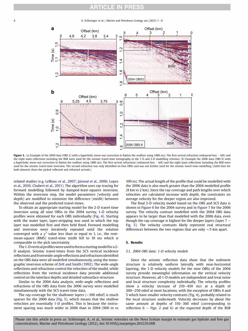
Figure 3. (a) Example of the 2004 data (OBS 2) with a hyperbolic move-out correction to flatten the seafloor using 1480 m/s. The first-arrival refraction (enhanced box e left) andthe eight main reflections including the BSR were used for the seismic travel-time tomography in the 1-D and 2-D modelling schemes. (b) Example the 2006 data (OBS 6) witha hyperbolic move-out correction to flatten the seafloor using 1480 m/s. The first-arrival refractions (enhanced box e left) and the eight main reflections including the BSR wereused for the seismic travel-time inversion. The second refraction was only identified on four OBSs and was not further used for the seismic travel-time modelling. (Solid lines forboth datasets show the picked reflected and refracted arrivals.)


related studies (e.g. LeBlanc et al., 2007; Jaiswal et al., 2006; Lopezet al., 2010; Chabert et al., 2011). The algorithm uses ray-tracing forforward modelling followed by damped-least-squares inversion.Within the inversion step, the model parameters (velocity anddepth) are modified to minimize the difference (misfit) betweenthe observed and the predicted travel-times.

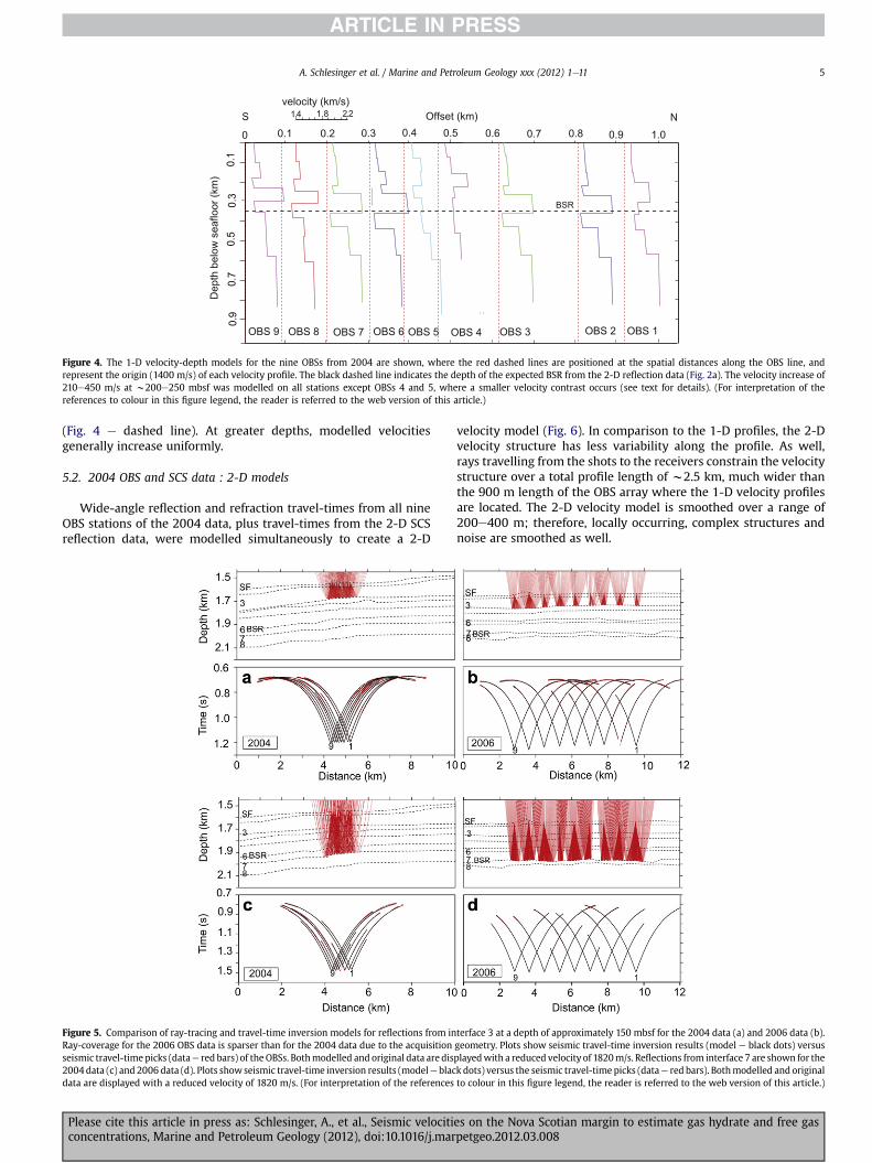
To obtain an appropriate starting model for the 2-D travel-timeinversion using all nine OBSs in the 2004 survey, 1-D velocityprofiles were obtained for each OBS individually (Fig. 4). Startingwith the water layer, layer-stripping was used in which the toplayer was modelled first and then held fixed. Forward modellingand inversion were iteratively repeated until the solutionconverged with a c2 value less than or equal to 1, i.e., the root-mean-square (RMS) travel-time misfit fell to 10 ms which iscomparable to the pick uncertainty.

The1-Dverticalprofileswereusedtoformastartingmodelfora2-D analysis. Seismic travel-times from the SCS vertical incidencereflectionsandfromwide-anglereflectionsandrefractionsidentifiedon the OBS data were all modelled simultaneously, using the tomo-graphic inversion scheme of Zelt and Smith (1992). The wide-anglereflections and refractions control the velocities of themodel, whilereflections from the vertical incidence data provide additionalcontrol on the interface depths and detailed subsurface structure.

Similar to the 2004 data analysis, wide-angle reflections andrefractions of the OBS data from the 2006 survey were modelledsimultaneously with the SCS travel-time data.

The ray-coverage for the shallower layers (<100 mbsf) is muchsparser for the 2006 data (Fig. 5), which means that the shallowvelocities are essentially 1-D profiles. This is because the instru-ment spacing was much wider in 2006 than in 2004 (900 m vs


100m). The actual length of the profile that could bemodelled withthe 2006 data is also much greater than the 2004 modelled profile(8 kmvs 2 km). Since the ray-coverage and path lengths over whichvelocities are calculated increase with depth, the constraints onaverage velocity for the deeper region are also improved.

The final 2-D velocity model based on the OBS and SCS data isshown in Figure 6 for the 2004 survey and in Figure 7 for the 2006survey. The velocity contrast modelled with the 2004 OBS dataappears to be larger than that modelled with the 2006 data, eventhough the ray-coverage is highest for the deeper layers (layer 7 e

Fig. 5). The velocity contrasts likely represent real structuraldifferences between the two regions that are only w5 km apart.

5. Results

5.1. 2004 OBS data: 1-D velocity models

Since the seismic reflection data show that the sedimentstructure is relatively uniform laterally with near-horizontallayering, the 1-D velocity models for the nine OBSs of the 2004survey provide meaningful information on the vertical velocitystructure. However, all 1-Dmodels are independent and treat noiseand local structure complexity individually. The velocity profilesshow a velocity increase of 210e450 m/s at a depth of200e250 mbsf at most locations, with the exception of OBSs 4 and5 which have smaller velocity contrasts (Fig. 4), probably related tothe local structure underneath. Velocity decreases by about thesame amount at depths of 310e360 mbsf (corresponding toreflection 6 e Figs. 2 and 6) at the expected depth of the BSR


0.9

0.7

0.5

0.3

0.1

S N

OBS 9 OBS 8 OBS 5OBS 6OBS 7 OBS 4 OBS 2 OBS 1OBS 3

0.1 0.2 0.3 0.4 0.60.5 0.7 0.80

Offset (km)

0.9

Dep

th b

elow

sea

floor

(km

)

2.21.4velocity (km/s)

1.0

1.8

BSR

Figure 4. The 1-D velocity-depth models for the nine OBSs from 2004 are shown, where the red dashed lines are positioned at the spatial distances along the OBS line, andrepresent the origin (1400 m/s) of each velocity profile. The black dashed line indicates the depth of the expected BSR from the 2-D reflection data (Fig. 2a). The velocity increase of210e450 m/s at w200e250 mbsf was modelled on all stations except OBSs 4 and 5, where a smaller velocity contrast occurs (see text for details). (For interpretation of thereferences to colour in this figure legend, the reader is referred to the web version of this article.)


(Fig. 4 e dashed line). At greater depths, modelled velocitiesgenerally increase uniformly.

5.2. 2004 OBS and SCS data : 2-D models

Wide-angle reflection and refraction travel-times from all nineOBS stations of the 2004 data, plus travel-times from the 2-D SCSreflection data, were modelled simultaneously to create a 2-D

Figure 5. Comparison of ray-tracing and travel-time inversion models for reflections from inRay-coverage for the 2006 OBS data is sparser than for the 2004 data due to the acquisitionseismic travel-time picks (datae red bars) of the OBSs. Bothmodelled and original data are dis2004 data (c) and 2006 data (d). Plots showseismic travel-time inversion results (modele blacdata are displayed with a reduced velocity of 1820 m/s. (For interpretation of the references


velocity model (Fig. 6). In comparison to the 1-D profiles, the 2-Dvelocity structure has less variability along the profile. As well,rays travelling from the shots to the receivers constrain the velocitystructure over a total profile length of w2.5 km, much wider thanthe 900 m length of the OBS array where the 1-D velocity profilesare located. The 2-D velocity model is smoothed over a range of200e400 m; therefore, locally occurring, complex structures andnoise are smoothed as well.

terface 3 at a depth of approximately 150 mbsf for the 2004 data (a) and 2006 data (b).geometry. Plots show seismic travel-time inversion results (model e black dots) versusplayedwith a reduced velocity of 1820m/s. Reflections from interface 7 are shown for thek dots) versus the seismic travel-time picks (datae red bars). Bothmodelled and originalto colour in this figure legend, the reader is referred to the web version of this article.)


1.40

1.50

1.60

1.70

1.80

1.90

Distance (km)4 5 6 7

Dep

th (k

m)

1.6

1.8

2.0

2.2

1.4

2004

SF

BSR

(km/s)NS

9 12345678

2.4

Velocity8

12

3

45

67

8

9

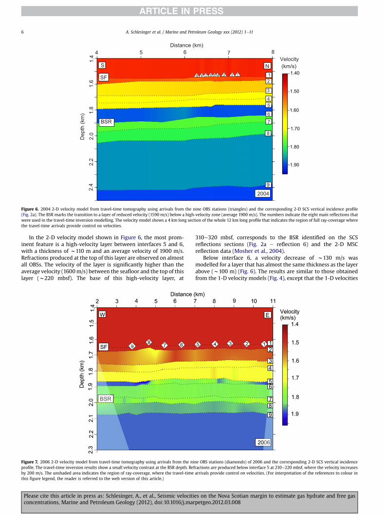
Figure 6. 2004 2-D velocity model from travel-time tomography using arrivals from the nine OBS stations (triangles) and the corresponding 2-D SCS vertical incidence profile(Fig. 2a). The BSR marks the transition to a layer of reduced velocity (1590 m/s) below a high-velocity zone (average 1900 m/s). The numbers indicate the eight main reflections thatwere used in the travel-time inversion modelling. The velocity model shows a 4 km long section of the whole 12 km long profile that indicates the region of full ray-coverage wherethe travel-time arrivals provide control on velocities.


In the 2-D velocity model shown in Figure 6, the most prom-inent feature is a high-velocity layer between interfaces 5 and 6,with a thickness of w110 m and an average velocity of 1900 m/s.Refractions produced at the top of this layer are observed on almostall OBSs. The velocity of the layer is significantly higher than theaverage velocity (1600m/s) between the seafloor and the top of thislayer (w220 mbsf). The base of this high-velocity layer, at

Figure 7. 2006 2-D velocity model from travel-time tomography using arrivals from the niprofile. The travel-time inversion results show a small velocity contrast at the BSR depth. Refby 200 m/s. The unshaded area indicates the region of ray-coverage, where the travel-timethis figure legend, the reader is referred to the web version of this article.)


310e320 mbsf, corresponds to the BSR identified on the SCSreflections sections (Fig. 2a e reflection 6) and the 2-D MSCreflection data (Mosher et al., 2004).

Below interface 6, a velocity decrease of w130 m/s wasmodelled for a layer that has almost the same thickness as the layerabove (w100 m) (Fig. 6). The results are similar to those obtainedfrom the 1-D velocity models (Fig. 4), except that the 1-D velocities

ne OBS stations (diamonds) of 2006 and the corresponding 2-D SCS vertical incidenceractions are produced below interface 5 at 210e220 mbsf, where the velocity increasesarrivals provide control on velocities. (For interpretation of the references to colour in



are less consistent laterally since each OBS was modelled inde-pendently. The velocity contrast at the BSR depth, achieved in the1-D velocity models, is larger (w300 m/s) than the contrastmodelled in the 2-D approach with the same data (w130 m/s).

Below interface 7, the velocity slowly increases to 1800 m/s forlayer 8 at a depth of 400 mbsf. With deep reflections on some of theOBSs, layer 9wasmodelledwith a velocity of 1900m/s and a base atw850 mbsf. No vertical incidence data are available to provideadditional constraints on the depth of this layer.

5.3. 2006 OBS and SCS data: 2D models

The final 2-D velocity model of the 2006 data simultaneouslyincorporated seismic travel-time arrivals from the nine OBSs andthe 2-D SCS vertical incidence profile (Fig. 7). The velocity increasesgradually, from 1490 m/s near the seafloor to 1650 m/s atw210 mbsf. At that depth, the modelled rays refract at the top ofa layer in which the velocity increases sharply to 1820 m/s in thecentral part of the profile, with indications of higher velocities(>1900 m/s) at the western and eastern ends. This layer hasa thickness of only 30e40 m, so its velocity is poorly constrained.However, beneath that interval a thicker (100 m) layer wasmodelled with similar velocities (1810e1840 m/s), so the

−12 −8 −4 0 4 8 12

3.5

4.5

5.5

6.5

7.5

Velocity perturbation (%)

RM

S (m

s)

2006

2004

−12 −8 −4 0 4 8 12

4

6

8

Velocity perturbation (%)

RM

S (m

s) 2006

200410

12

14

16a

b

Figure 8. (a) Results of the sensitivity analysis of the 2004 (dashed line) and 2006(solid line) OBS data for the velocity perturbation of the high-velocity layer above theidentified BSR. An approximate estimate of the confidence range for both OBS datasetsis indicated by the shaded box. (b) Results of the sensitivity analysis of the 2004(dashed line) and 2006 (solid line) OBS data for the velocity perturbation of the low-velocity layer below the identified BSR depth. Allowed velocity perturbations are �3%for the 2004 data (shaded box), but much greater (>�5%) for the 2006 data.


transition to higher velocities over this depth range is well-established. The high-velocity layer extends downward to inter-face 7 at a depth of w330 mbsf, corresponding to the BSR asidentified in the 2-D SCS and 2-DMCS sections (Mosher et al., 2004)(Fig. 2b). Below interface 7, the velocity model shows a smallvelocity decrease of 50e70 m/s that contrasts with the largervelocity decrease modelled in the 2004 data.

5.4. Sensitivity analysis for layers above and below BSRs

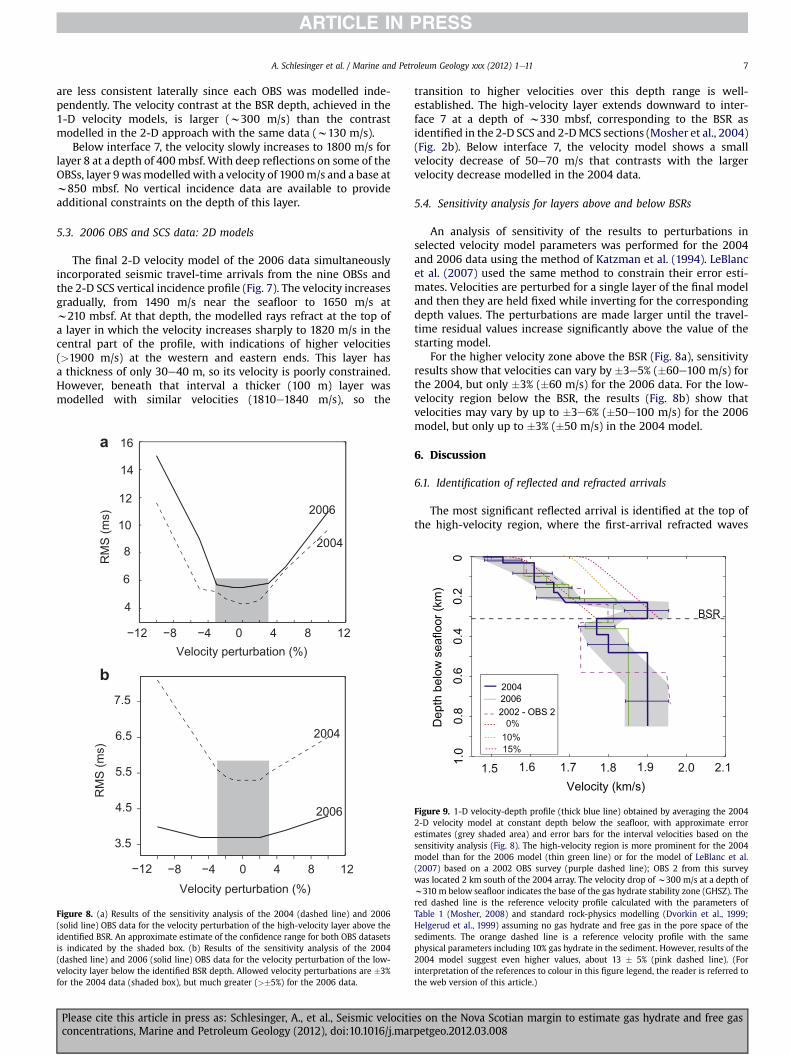
An analysis of sensitivity of the results to perturbations inselected velocity model parameters was performed for the 2004and 2006 data using the method of Katzman et al. (1994). LeBlancet al. (2007) used the same method to constrain their error esti-mates. Velocities are perturbed for a single layer of the final modeland then they are held fixed while inverting for the correspondingdepth values. The perturbations are made larger until the travel-time residual values increase significantly above the value of thestarting model.

For the higher velocity zone above the BSR (Fig. 8a), sensitivityresults show that velocities can vary by �3e5% (�60e100 m/s) forthe 2004, but only �3% (�60 m/s) for the 2006 data. For the low-velocity region below the BSR, the results (Fig. 8b) show thatvelocities may vary by up to �3e6% (�50e100 m/s) for the 2006model, but only up to �3% (�50 m/s) in the 2004 model.

6. Discussion

6.1. Identification of reflected and refracted arrivals

The most significant reflected arrival is identified at the top ofthe high-velocity region, where the first-arrival refracted waves

0

Velocity (km/s)1.6 1.7 1.8 1.9 2.01.5 2.11.

00.

80.

60.

40.

2D

epth

bel

ow s

eaflo

or (k

m)

BSR

20062002 - OBS 2

2004

0% 10% 15%

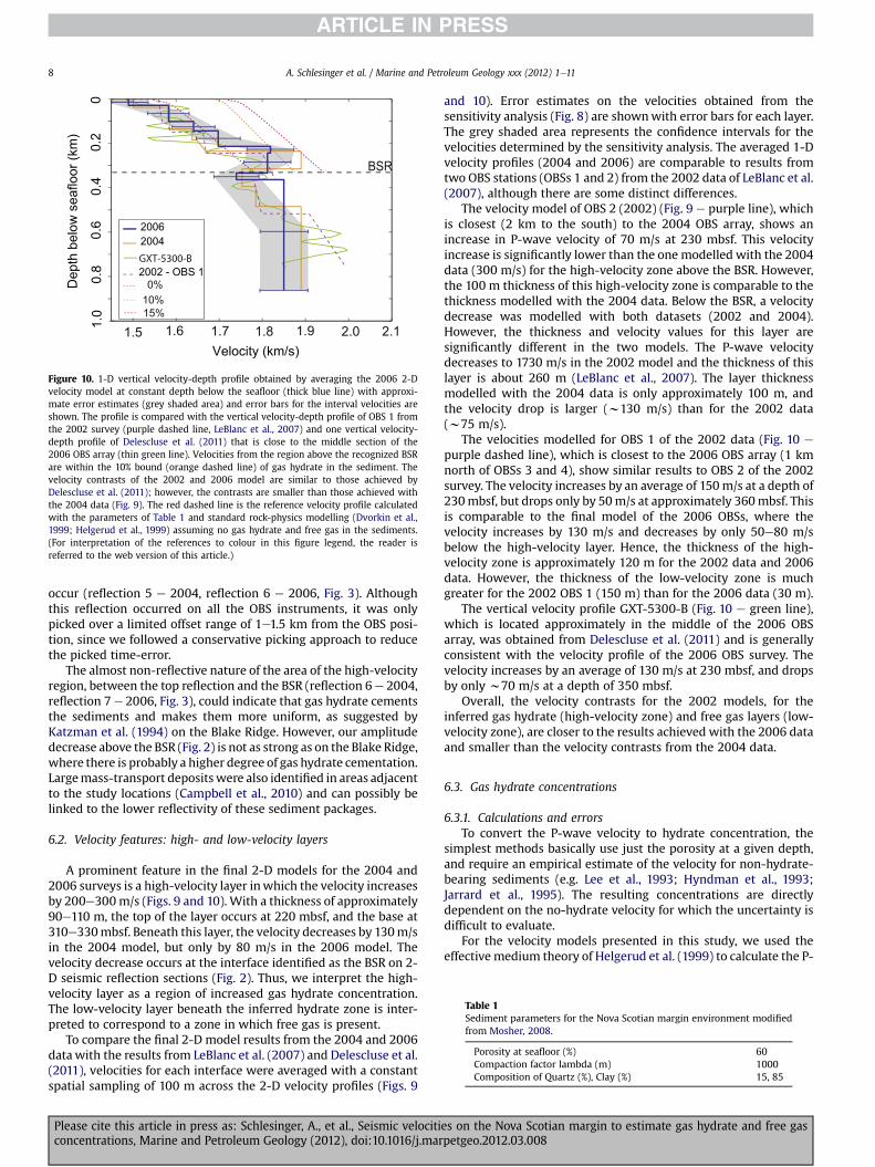
Figure 9. 1-D velocity-depth profile (thick blue line) obtained by averaging the 20042-D velocity model at constant depth below the seafloor, with approximate errorestimates (grey shaded area) and error bars for the interval velocities based on thesensitivity analysis (Fig. 8). The high-velocity region is more prominent for the 2004model than for the 2006 model (thin green line) or for the model of LeBlanc et al.(2007) based on a 2002 OBS survey (purple dashed line); OBS 2 from this surveywas located 2 km south of the 2004 array. The velocity drop of w300 m/s at a depth ofw310 m below seafloor indicates the base of the gas hydrate stability zone (GHSZ). Thered dashed line is the reference velocity profile calculated with the parameters ofTable 1 (Mosher, 2008) and standard rock-physics modelling (Dvorkin et al., 1999;Helgerud et al., 1999) assuming no gas hydrate and free gas in the pore space of thesediments. The orange dashed line is a reference velocity profile with the samephysical parameters including 10% gas hydrate in the sediment. However, results of the2004 model suggest even higher values, about 13 � 5% (pink dashed line). (Forinterpretation of the references to colour in this figure legend, the reader is referred tothe web version of this article.)


01.

00.

80.

60.

40.

2

Dep

th b

elow

sea

floor

(km

)

Velocity (km/s)1.6 1.7 1.8 1.9 2.01.5 2.1

2006

2002 - OBS 1 0% 10% 15%

BSR

2004

Figure 10. 1-D vertical velocity-depth profile obtained by averaging the 2006 2-Dvelocity model at constant depth below the seafloor (thick blue line) with approxi-mate error estimates (grey shaded area) and error bars for the interval velocities areshown. The profile is compared with the vertical velocity-depth profile of OBS 1 fromthe 2002 survey (purple dashed line, LeBlanc et al., 2007) and one vertical velocity-depth profile of Delescluse et al. (2011) that is close to the middle section of the2006 OBS array (thin green line). Velocities from the region above the recognized BSRare within the 10% bound (orange dashed line) of gas hydrate in the sediment. Thevelocity contrasts of the 2002 and 2006 model are similar to those achieved byDelescluse et al. (2011); however, the contrasts are smaller than those achieved withthe 2004 data (Fig. 9). The red dashed line is the reference velocity profile calculatedwith the parameters of Table 1 and standard rock-physics modelling (Dvorkin et al.,1999; Helgerud et al., 1999) assuming no gas hydrate and free gas in the sediments.(For interpretation of the references to colour in this figure legend, the reader isreferred to the web version of this article.)

Table 1Sediment parameters for the Nova Scotian margin environment modifiedfrom Mosher, 2008.

Porosity at seafloor (%) 60Compaction factor lambda (m) 1000Composition of Quartz (%), Clay (%) 15, 85


occur (reflection 5 e 2004, reflection 6 e 2006, Fig. 3). Althoughthis reflection occurred on all the OBS instruments, it was onlypicked over a limited offset range of 1e1.5 km from the OBS posi-tion, since we followed a conservative picking approach to reducethe picked time-error.

The almost non-reflective nature of the area of the high-velocityregion, between the top reflection and the BSR (reflection 6e 2004,reflection 7 e 2006, Fig. 3), could indicate that gas hydrate cementsthe sediments and makes them more uniform, as suggested byKatzman et al. (1994) on the Blake Ridge. However, our amplitudedecrease above the BSR (Fig. 2) is not as strong as on the Blake Ridge,where there is probably a higher degree of gas hydrate cementation.Largemass-transport depositswere also identified in areas adjacentto the study locations (Campbell et al., 2010) and can possibly belinked to the lower reflectivity of these sediment packages.

6.2. Velocity features: high- and low-velocity layers

A prominent feature in the final 2-D models for the 2004 and2006 surveys is a high-velocity layer inwhich the velocity increasesby 200e300m/s (Figs. 9 and 10). With a thickness of approximately90e110 m, the top of the layer occurs at 220 mbsf, and the base at310e330mbsf. Beneath this layer, the velocity decreases by 130m/sin the 2004 model, but only by 80 m/s in the 2006 model. Thevelocity decrease occurs at the interface identified as the BSR on 2-D seismic reflection sections (Fig. 2). Thus, we interpret the high-velocity layer as a region of increased gas hydrate concentration.The low-velocity layer beneath the inferred hydrate zone is inter-preted to correspond to a zone in which free gas is present.

To compare the final 2-D model results from the 2004 and 2006datawith the results from LeBlanc et al. (2007) and Delescluse et al.(2011), velocities for each interface were averaged with a constantspatial sampling of 100 m across the 2-D velocity profiles (Figs. 9


and 10). Error estimates on the velocities obtained from thesensitivity analysis (Fig. 8) are shownwith error bars for each layer.The grey shaded area represents the confidence intervals for thevelocities determined by the sensitivity analysis. The averaged 1-Dvelocity profiles (2004 and 2006) are comparable to results fromtwo OBS stations (OBSs 1 and 2) from the 2002 data of LeBlanc et al.(2007), although there are some distinct differences.

The velocity model of OBS 2 (2002) (Fig. 9 e purple line), whichis closest (2 km to the south) to the 2004 OBS array, shows anincrease in P-wave velocity of 70 m/s at 230 mbsf. This velocityincrease is significantly lower than the one modelled with the 2004data (300 m/s) for the high-velocity zone above the BSR. However,the 100 m thickness of this high-velocity zone is comparable to thethickness modelled with the 2004 data. Below the BSR, a velocitydecrease was modelled with both datasets (2002 and 2004).However, the thickness and velocity values for this layer aresignificantly different in the two models. The P-wave velocitydecreases to 1730 m/s in the 2002 model and the thickness of thislayer is about 260 m (LeBlanc et al., 2007). The layer thicknessmodelled with the 2004 data is only approximately 100 m, andthe velocity drop is larger (w130 m/s) than for the 2002 data(w75 m/s).

The velocities modelled for OBS 1 of the 2002 data (Fig. 10 e

purple dashed line), which is closest to the 2006 OBS array (1 kmnorth of OBSs 3 and 4), show similar results to OBS 2 of the 2002survey. The velocity increases by an average of 150m/s at a depth of230mbsf, but drops only by 50m/s at approximately 360mbsf. Thisis comparable to the final model of the 2006 OBSs, where thevelocity increases by 130 m/s and decreases by only 50e80 m/sbelow the high-velocity layer. Hence, the thickness of the high-velocity zone is approximately 120 m for the 2002 data and 2006data. However, the thickness of the low-velocity zone is muchgreater for the 2002 OBS 1 (150 m) than for the 2006 data (30 m).

The vertical velocity profile GXT-5300-B (Fig. 10 e green line),which is located approximately in the middle of the 2006 OBSarray, was obtained from Delescluse et al. (2011) and is generallyconsistent with the velocity profile of the 2006 OBS survey. Thevelocity increases by an average of 130 m/s at 230 mbsf, and dropsby only w70 m/s at a depth of 350 mbsf.

Overall, the velocity contrasts for the 2002 models, for theinferred gas hydrate (high-velocity zone) and free gas layers (low-velocity zone), are closer to the results achieved with the 2006 dataand smaller than the velocity contrasts from the 2004 data.

6.3. Gas hydrate concentrations

6.3.1. Calculations and errorsTo convert the P-wave velocity to hydrate concentration, the

simplest methods basically use just the porosity at a given depth,and require an empirical estimate of the velocity for non-hydrate-bearing sediments (e.g. Lee et al., 1993; Hyndman et al., 1993;Jarrard et al., 1995). The resulting concentrations are directlydependent on the no-hydrate velocity for which the uncertainty isdifficult to evaluate.

For the velocity models presented in this study, we used theeffective medium theory of Helgerud et al. (1999) to calculate the P-



wave velocity for a given gas hydrate concentration. Chand et al.(2004) evaluated a number of different effective medium theo-ries, in which they calculated sediment physical properties fromestimates of the porosity, clay-content and quartz-content. Themodels predicted similar variations of P-wave velocity with hydrateconcentration, but the most consistent values for the no-hydratevelocity were found using the theories of Helgerud et al. (1999)and Jakobsen et al. (2000). The calculations were validated bycomparisons with velocities determined from drill holes usingindependent methods. The geological environments testedincluded both sand-rich sediments (Mackenzie Delta) and clay-richsediments (Blake Ridge, where sediment compositions are similarto those on the Nova Scotia margin). In our calculations on theScotia margin, the sediment parameters were taken from LeBlancet al. (2007) (Table 1). Using effective medium theory, we calcu-lated a reference velocity profile corresponding to no gas hydrate orfree gas in the pore space (Figs. 9 and 10 e fine red dashed line),plus two other profiles inwhich the bulk gas hydrate concentrationis 10% and 15% (Figs. 9 and 10).

The calculated gas hydrate concentrations for the 2006modelled velocities are approximately 2e11% of the pore space.These values are slightly larger than the 2e6% concentrationsof bulk gas hydrate estimated from the nearby OBS 1 in the studyof LeBlanc et al. (2007). However, the modelled velocities for the2004 data are higher, corresponding to a greater gas hydrateconcentration of approximately 8e18% in the pore space. This isour best estimate of the concentration range for the 2004 data,corresponding to an approximate velocity uncertainty of �75 m/s;however, a larger range cannot be excluded since our sensitivityanalysis provides only a rough velocity uncertainty of�50e100 m/s.

The reference profile for no gas hydrate is not explicitly includedin the error estimate above, which deals with just velocity uncer-tainties. The concentration is also dependent on specific physicalparameters of the sediments, such as the seafloor porosity and thecompaction factor, which defines the rate of the depth-dependentporosity decrease (Table 1). For example, if the seafloor porosityis decreased by 3%, the calculated reference velocity profile for nogas hydrate increases by w50 m/s, so it is near the upper bound ofour confidence limit for the no-hydrate region above 220 mbsf.Hence, the calculated gas hydrate concentrations would showa decrease of 2% compared to the ranges calculated above. Incontrast, increasing the seafloor porosity by 3% decreases theaverage reference velocities by 30 m/s, but the calculated values forgas hydrate concentration increase by w10%. Therefore, we feelthat our selected seafloor porosity of 60%, based on LeBlanc et al.(2007), represents a conservative estimate for gas hydrateconcentrations.

6.3.2. Lateral variation in hydrate concentrationThe OBS sites of this study are located near the eastern sidewall

of the Mohican Channel (Fig. 1). The 2004 OBS array, oriented northto south, is parallel and very close to the channel wall, whereas the2006 OBS array is oriented west to east, perpendicular to thechannel wall and extending away from it. In the final 2-D velocitymodels, velocity values and calculated gas hydrate concentrationsfor the layer above the BSR are significantly higher for the 2004data than for the 2006 data. That is, gas hydrate concentrationsgenerally appear to decrease with distance from the MohicanChannel. This pattern is consistent with the 2e6% gas hydrateconcentrations derived for the 2002 data for OBS 1, located east ofthe channel (LeBlanc et al., 2007). Here, the decreasing gas hydrateconcentrations with increasing distance from the channel isexplained as an effect of lower porosity within the mud-dominantsediment at the depth of the BSR.


A similar pattern was observed in the 2-D reflection seismicdatasets, for which BSRs occur in patches distributed over theScotian margin, and are mainly located where channel structuresappear (Cullen et al., 2008; Mosher, 2011). Although most of theScotian margin sediments are fine-grained, glacially-derived,marine sediments with a high percentage of clay (Mosher, 2008),coarser grained deposits were probably transported in the outwashchannels (e.g. Mohican Channel) and deposited over the sidewallsand foot of the channel.

Mosher (2011) stated that most of the recognized BSRs arewithin large sedimentary drift deposits that were transportedduring the Miocene and Pliocene (Campbell et al., 2010). Recentstudies show that the Pleistocene-to-recent Mohican Channel cutsthrough these deposits, exhibiting various episodes of cut-and-fillduring this period (Campbell et al., 2010; Mosher, 2011). Theoccurrence of gas hydrate is likely linked to grain-sorting andporosity changes that establish potential reservoir rocks along theMohican Channel.

Recent studies from the Svalbard margin by Chabert et al. (2011)show similar results, where the formation of gas hydrate iscontrolled by lithology, which varies downslope from glacial-marine sediments to finer hemipelagic sediments. According toChabert et al. (2011), gas hydrate concentrations in glacial-marinesediments are too small to produce a prominent increase in P-wave velocity. Estimated gas hydrate concentrations within thesediment frame, modelled using effective medium modelling(Helgerud et al., 1999) amongst others, range between 5% and 12%(Chabert et al., 2011). Another study from the mid-Norwegianmargin by Bünz et al. (2005) shows a discontinuous BSR alongthe margin at the Storegga slide. Gas hydrate estimates are withina range of 3e6% of the pore space assuming hydrate asa component of the sediment frame using effective mediummodelling (Bünz et al., 2005).

A key feature of the gas hydrate distribution on the passiveScotian margin, based on the seismic velocity analyses, is that thehydrate is distributed in the w100 m thick region just above theBSR, with no indications of gas hydrate occurring between theseafloor and the top of that layer (w220 mbsf). Malinverno et al.(2008) presented modelling results from the Cascadia margin toshow that this could be produced, either by low sedimentationrates or by low rates of diffusive upward fluid flow. On the passiveScotian margin, the low fluid flux rates are likely the dominantfactor in restricting gas hydrate to the layer above the BSR.

6.4. Free gas concentrations

Laboratory studies (e.g. Lee, 2004) show that very smallconcentrations of free gas in the pore space can have a large velocityeffect. Concentrations as small as 1% can reduce the P-wave velocityby more than 5%, or approximately 90 m/s (LeBlanc et al., 2007).Those free gas concentrations were calculated based on the rock-physics models presented by Helgerud et al. (1999) and Dvorkinet al. (1999). Similar velocity decreases of 50e80 m/s, as modelledwith the 2006 dataset, and 130 m/s, modelled with the 2004dataset, correspond to concentrations of 1e2% gas in thesediments at depths of 310e330 mbsf. The modelled thickness forthis low-velocity layer beneath the BSR is approximately 30e150m.

Our results for gas zone thickness are consistent with Xu andRuppel (1999) and Haacke et al. (2008), who argue that a thickfree gas zone is associated with passive margins with low rates ofmethane flux (<few tenths mm/yr, Haacke et al., 2007) and slowerseafloor uplift, in contrast to active margins where a thin free gaszone (w10e30 m) is produced with high rates of upward directedfluid flux (>few tenths of mm/yr, Haacke et al., 2007) and high ratesof seafloor uplift (e.g., accretionary wedges).



The 1-D vertical velocity profiles obtained by Delescluse et al.(2011) show smaller contrasts between the two velocity zones atthe BSR depth with increasing distance from the Mohican Channel.In addition to the velocity profile GXT-5300-B (Fig. 10), Delescluseet al. (2011) modelled another vertical velocity profile that islocated several kilometres to the west of the 2006 OBS array, at theedge of the Mohican Channel. The results show a velocity decreaseof 200 m/s below the BSR depth. The lower velocity is most likelya result of higher gas concentrations within the sediments that arecloser to the Mohican Channel.

6.5. OBS surveys

As the final velocity models of both surveys (2004 and 2006)show, the geometry for OBS surveys is crucial to the obtainedresults. Choosing the appropriate instrument spacing (<500 m) isessential for modelling the velocity contrasts produced by evensmall amounts of gas hydrate in the pore space of shallow sedi-ments. Large shot offsets (>5 km) to both sides of the instrumentsare also necessary to detect refracted and wide-angle reflectedarrivals from below the BSR that constrain the velocities in thesedeep regions.

7. Conclusions

The velocity structure beneath the Scotian margin off easternCanada was modelled in a travel-time inversion approach usingocean-bottom seismometer and single-channel seismic data.Careful analysis and modelling permitted the small velocityanomalies associated with low concentrations of gas hydrate andfree gas to be resolved. A high-velocity zone, occurring over thedepth range of w220e330 mbsf with a modelled velocity increaseof 200e300m/s, is interpreted as a gas hydrate layer. Depending onthe chosen rock-physics model and a depth-dependent no gashydrate background velocity model, the modelled velocity increaseimplies gas hydrate concentrations of 4e13% of the pore space. Thepresumed gas hydrate is located just above the identified bottom-simulating reflection. The region between the seafloor and thetop of the gas hydrate layer (w220 mbsf) shows no indications ofgas hydrate, which may be explained by the low diffusive fluid fluxrates common for passive margins (e.g. Haacke et al., 2007). Basedon results from three seismic surveys between 2002 and 2006, gashydrate concentrations generally decrease with relative distancefrom the Mohican channel structure. The decreasing velocitycontrast at the BSR depth with relative distance from the MohicanChannel, as concluded by Delescluse et al. (2011), strengthens thisargument.

Beneath the bottom-simulating reflection, the velocitydecreases by approximately 130 m/s, which corresponds to freegas concentrations of 1e2% of the sediment pore space. Thethickness of the free gas layer is 30e150 m, which is significantlygreater than for most active continental margins (10e30 m). Thelow concentrations and thicker layer for this passive margin areprobably a consequence of the low upward directed fluid fluxrates.

Acknowledgements

The authors thank the crew and staff of CCGS Hudson for theirdedication in acquiring the seismic data used in this study. Thework was supported by grants from the Natural Science andEngineering Research Council to K. Louden, D. Mosher, R.Hyndman and G. Spence, and from the Climate Change Technologyand Innovation (CCTI) program to R. Hyndman. Natural ResourcesCanada, Earth Science Sector, Gas Hydrate: Fuel for the Future


program funded the research expeditions to acquire the data usedin this study. The Climate Change Technology and InnovationResearch and Development Initiative, Natural Resources Canada,partially funded development of the ocean-bottom seismometers(OBS).

Further thanks go to Christan Berndt, Michael Riedel and ananonymous reviewer for their helpful ideas and criticism. Velocityfigures and maps were prepared with GMT software (Wessel andSmith, 1995) and seismic data were processed and plotted usingthe Seismic Unix software.

References

Bünz, S., Mienert, J., Vanneste, M., Andreassen, K., 2005. Case Study. Gas hydrates atthe Storegga Slide: constraints from an analysis of multicomponent, wide-angleseismic data. Geophysics 70 (5), B19eB34.

Campbell, C.D., Mosher, D.C., Shimeld, J.W., 2010. Erosional unconformities, mega-slumps and giant mud waves: insights into passive margin evolution from thecontinental slope off Nova Scotia. In: Central and North American ConjugateMargins Conference: Re-discovering the Atlantic, New Winds from an Old Sea,Lisbon 2010, vol. IV, pp. 37e41.

Chabert, A., Minshull, T.A., Westbrook, G.K., Berndt, C., Thatcher, K.E., Sarkar, S.,2011. Characterization of a stratigraphically constrained gas hydrate systemalong the western continental margin of Svalbard from ocean bottom seis-mometer data. Journal of Geophysical Research 116, 16.

Chand, S., Minshull, T.A., Gei, D., Carcione, J.M., 2004. Elastic velocity models for gas-hydrate-bearing sediments–a comparison. Geophysical Journal International159 (2), 573e590.

Cullen, J., Mosher, D.C., Louden, K.E., 2008. The Mohican channel gas hydrate zone,Scotian Slope, Geophysical structure. In: Proceedings of the 6th InternationalConference on Gas Hydrates (ICGH2008).

Dai, J., Xu, H., Snyder, F., Dutta, N., 2004. Detection and estimation of gas hydratesusing rock physics and seismic inversion: examples from the northern deep-water Gulf of Mexico. The Leading Edge 23 (1), 60e66.

Delescluse, M., Nedimovic, M.R., Louden, K.E., 2011. Case History e 2D waveformtomography applied to long-streamer MCS data from the Scotian Slope.Geophysics 76 (4), B151eB163.

Dvorkin, J., Prasad, M., Sakai, A., Lavoie, D., 1999. Elasticity of marine sediments:rock physics modelling. Geophysical Research Letters 26 (12), 1781e1784.

Haacke, R.R., Westbrook, G., Hyndman, R., 2007. Gas hydrate, fluid flow and free gas:formation of the bottom-simulating reflector. Earth and Planetary ScienceLetters 261, 407e420, 17 pp.

Haacke, R.R., Westbrook, G., Riley, M., 2008. Controls on the formation andstability of gas hydrate related bottom-simulating reflectors (BSRs): a casestudy from the west Svalbard continental slope. Journal of GeophysicalResearch 113.

Helgerud, M.B., Dvorkin, J., Nur, A., Sakai, A., Collett, T., 1999. Elastic-wave velocity inmarine sediments with gas hydrates: effective medium modelling. GeophysicalResearch Letters 26 (13), 2021e2024.

Holbrook, W.S., Hoskins, H., Wood, W.T., Stephen, R.A., Lizarrade, D., 1996. Methanehydrate, bottom-simulating reflectors, and gas bubbles: results of verticalseismic profiles on the Blake Ridge. Science 273, 1840e1843.

Hyndman, R.D., Moore, G.F., Moran, K., 1993. Velocity, porosity, and pore-fluid lossfrom the Nankai subduction zone accretionary prism. In: Hill, I.A., Taira, A.,Firth, J.V., et al. (Eds.), 1993. Proceedings of the Ocean Drilling Program,Scientific Results, vol. 131, College Station, TX, pp. 211e220.

Jakobsen, M., Hudson, J.A., Minshull, T.A., Singh, S.C., 2000. Elastic properties ofhydrate-bearing sediments using effective medium theory. Journal ofGeophysical Research 105, 561e577.

Jaiswal, P., Zelt, C.A., Pecher, I.A., 2006. Seismic characterization of a gas hydratesystem in the Gulf of Mexico using wide-aperture data. Geophysical JournalInternational 165, 108e120.

Jarrard, R.D., MacKay, M.E., Westbrook, G.K., Screaton, E.J., 1995. Log-based porosityof ODP sites on the Cascadia accretionary prism. In: Carson, B., Westbrook, G.K.,Musgrave, R.J., Suess, E. (Eds.), Proceedings of the Ocean Drilling Program,Scientific Results, 146 (Part 1), College Station, TX, pp. 313e335.

Katzman, R., Holbrook, W.S., Paull, C.K., 1994. Combined vertical-incidence andwide-angle seismic study of a gas hydrate zone, Blake Ridge. Journal ofGeophysical Research 99, 17,975e17,995.

LeBlanc, C., Louden, K., Mosher, D., 2007. Gas hydrates off Eastern Canada: velocitymodels from wide-angle seismic profiles on the Scotian Slope. Marine andPetroleum Geology 24, 321e335.

Lee, M.W., Hutchinson, D.R., Dillon, W.P., Miller, J.J., Agena, W.F., Swift, B.A., 1993.Method of estimating the amount of in-situ gas hydrates in deep marinesediments. Marine and Petroleum Geology 10 (5), 493e506.

Lee, M.W., 2004. Elastic velocities of partially gas-saturated unconsolidated sedi-ments. Marine and Petroleum Geology 21, 641e650.

Lopez, C., Spence, G., Hyndman, R., Kelley, D., 2010. Frontal ridge slope failure at thenorthern Cascadia margin: margin-normal fault and gas hydrate control.Geology 38 (11). doi:10.1130/G31136.1.



Malinverno, A., Kastner, M., Torres, M.E., Wortmann, U.E., 2008. Gas hydrateoccurrence from pore water chlorinity and downhole logs in transect across thenorthern Cascadia margin (Integrated Ocean Drilling Program Expedition).Journal of Geophysical Research 1 (13), B08103.

Mosher, D.C., Piper, D.J., Campbell, D.C., Jenner, K.A., 2004. Near surface geology andsediment-failure geohazards of the central Scotian Slope. AAPG 88, 703e723.

Mosher, D., 2004. Hudson 2004-030 Cruise Report: July 10e20, 2004. GeologicalSurvey of Canada (Atlantic), Open File, 72 p.

Mosher, D., 2008. Bottom simulating reflectors on Canada’s east coast margin:evidence for gas hydrate. In: Proceedings of the 6th International Conference onGas Hydrates (ICGH 2008).

Mosher, D., 2011. A margin-wide BSR gas hydrate assessment: Canada’s Atlanticmargin. Marine and Petroleum Geology 28 (8), 1540e1553.

Neave, K.G., 1990. Shallow seismic velocities on the eastern Grand Banks andFlemish Pass. Unpublished report Prepared for Alan Judge of the TerrainSciences Division, Geological Survey of Canada, 19 p.


Ruppel, C., Collett, T., Boswell, R., Lorenson, T., Buczkowski, B., Waite, W., 2011.A new global gas hydrate drilling map based on reservoir type. Fire in the Ice,DOE NETL Newsletter 11 (1), 13e17.

Tucholke, B.E., Bryan, G.M., Ewing, J.I., 1977. Gas hydrate horizons detected inseismic-profiler data from the western North Atlantic. American Association ofPetroleum Geologists Bulletin 61, 689e707.

Wessel, P, Smith, W.H.F., 1995. New version of the Generic Mapping Tool released.Eos, Transactions of the American Geophysical Union 76 (33), 329.

Xu, W., Ruppel, C., 1999. Predicting the occurrence, distribution, and evolution ofmethane gas hydrate in porous marine sediments from analytical models.Journal of Geophysical Research 104, 5081e5096.

Zelt, C.A., Smith, R.B., 1992. Seismic travel-time inversion for 2-D crustal velocitystructure. Geophysical Journal International 108, 16e34.

Zykov, M., 2006. 3-D travel time tomography of the gas hydrate area offshoreVancouver Island based on OBS data. PhD Thesis with the University of Victoria,BC, Canada.


Documents

Marine and Petroleum Geology - Web hosting