#2012

Asymptotic Optimality of the Least-Squares Cross-Validation Bandwidth

for Kernel Estimates of Intensity Functions

Maria Mori Brooks and J. Stephen Marron1

Department of Statistics. University of North Carolina.

Chape I Hi 11. NC 27599-3260. USA

November 16. 1989

ABSfRACf

In this paper. kernel function methods are considered for

estimating the intensity function of a nonhomogeneous Poisson process.

The bandwidth controls the smoothness of the kernel estimator. and

therefore. it is desirable to find a data-based bandwidth selection

method that performs well in some sense. It will be proven that the

least-squares cross-validation bandwidth is asymptotically optimal for

kernel intensity estimation.

Keywords: bandwidth selection. intensity function. cross-validation

bandwidth. kernel estimation. nonstationary Poisson processes.

1Research partially supported by NSF Grant DMS-8902973

1

1. Introduction

Let Xl' X2'.· ..~ be ordered observations on the interval [O.T]

from a nonstationary Poisson process with intensity function ~(x). In

this paper, we consider estimation of the intensity function ~(x). N.

the number of observations that occur in the interval [O,T]. has a

TPoisson distribution with E[N] = f O ~(u) du. See Cox and Isham (1980).

Ripley (1981). and Diggle (1983) for further information regarding point

processes.

Rosenblatt (1956) introduced a kernel density estimator for

independent identically distributed observations, Xl' X2 .... ,Xn , from an

unknown probability distribution f(x). The kernel density estimator is

defined as:

-1= nn

}; ~(x-Xi)i=l

(1. 1)

-1where ~(x) = h K(x/h). The kernel function. K(.). is the "shape" of

the weight that is placed on each data point. The smoothing parameter,

h. also known as the bandwidth, quantifies the smoothness of fh(x).

Using the same motivation, a natural estimate for ~(x) is the kernel

estimator:

The kernel function is assumed here to be a

N~(x) = };

i=l-1

where ~(x) = h K(x/h).

XE,[O,T] (1.2)

symmetric probability density function, and h is the smoothing parameter

for ~(x). Both of these estimators are appealing since they take on

large values in areas where the data are dense and small values where

the data are s~rse. The kernel density estimator includes a

2

-1normalization factor. n so that fh(x) is a probability density

function; this adjustment is not needed for estimating an intensity

function. Theoretical properties of the kernel intensity estimator have

been developed by Devroye and Gyorfi (1984). Leadbetter and Wold (1983).

and Ramlau-Hansen (1983a).

The choice of the smoothing parameter is usually far more important

than the choice of the kernel function for both kernel density and

intensity estimators. See Silverman (1986) for a discussion and

examples illustrating this point. Rosenblatt (1971) presented an

intuitive description for the tradeoff between smaller and larger values

of h. The mean square error (MSE) of ~h(x) is the sum of the squaredA

bias and the variance of ~h(x). Rosenblatt showed that a small value of

h results in high variance; ~h(x) is affected by individual observations

and hence is more variable. On the other hand. a large value of h

results in high bias; ~h(x) is very smooth but does not include minor

features of the true intensity function. Thus. it is desirable to find

a data-based bandwidth that balances the effects of the bias and the

variance of the estimate.

Two models are considered here for the intensity function. a simple

multiplicative intensity model and a stationary Cox process model. The

general multiplicative intensity model. introduced by Aalen (1978). is

frequently used to model counting processes. See Anderson and Borgan

(1985) for an overview of these models. Diggle (1985) studied the

kernel intensity estimator. ~(x). under the stationary Cox processA

model. He calculated the mean square error of ~h(x) using empirical

3

Bayesian methods and then estimated the "optimal" bandwidth by

minimizing an estimate of the MSE over h. When Ah(X) is used with a

uniform kernel, Diggle and Marron (1988) proved that Diggle's (1985)

minimum MSE method and the least-squares cross-validation bandwidth

selection method choose the same bandwidth.

For the related setting of kernel density estimation, Hall (1983),

Burman (1985), and Stone (1984) have proven that the least-squares

cross-validation bandwidth is asymptotically optimal. In this paper, we

show that the least-squares cross-validation method is also

asymptotically optimal for intensity estimation under both models. In

Section 2, we discuss the two intensity models. Section 3 contains the

main result regarding the asymptotic optimality of the least-squares

cross-validation bandwidth. Finally, the proof of the theorem is

presented in Section 4.

2. The Mathematical Models for the Intensi ty Function

We focus on two mathematical models for the intensity function: a

simple multiplicative intensity model and a stationary Cox process

model.

The simple multiplicative intensity model is a specific form of

Aalen's (1978) multiplicative intensity model. Suppose that

Xl' X2'···~ are observations from a nonhomogeneous Poisson process with

intensity

A (x) = c a(x)cx~[O,T] (2.1)

where c is a constant, and a(x) is an unknown nonnegative deterministic

4

function with fb a(x) dx = 1. Given N, the occurrence times,

Xl' X2 ,·· .,XN, have the same distribution as the order statistics

corresponding to N independent random variables with probability density

function a(x) on the interval [O,T]. The kernel estimate of A (x) isc

given in (1.2); under this model, N is a Poisson random variable that

has expected value equal to c. It follows from Ramlau-Hansen (1983a)

that this estimator is uniformly consistent and asymptotically normal

under the simple multiplicative intensity model.

The second model that we consider is the stationary Cox process

model. Let Xl' X2 , .. "XN form a realization of a stationary Cox process

on [O,T] with intensity function A (x) where ~ is discussed below.~

stationary Cox process (also known as a doubly stochastic Poisson

process) is defined by

A

1) {A(x), xcffi} is a stationary, non-negative valued random process

2) conditional on the realization A (x) of A(x), the point process~

is a nonhomogeneous Poisson process with rate function A (x).~

See Cox and Isham (1980) for a discussion of doubly stochastic Poisson

processes. We also assume that:

3) E[A(x)] = ~ where ~ is a constant,

4) E[A(x)A(y)] = v(lx-YI) where vex) = ~2 v (x)o

for v (x) a fixed function.o

This model is identical to the stationary Cox process model used in

Diggle (1985). The kernel estimate of A (x) in the Cox process model is~

the same as Ah(x) in the multiplicative intensity model for estimating

the intensity function from a data set. The difference between the two

5

models is only seen when the estimators are evaluated mathematically.

Under the Cox process model, N is a random variable such that

TE[N] = E[SO A(x) dx] = ~T.

Asymptotic analysis provides a powerful tool for understanding the

behavior of the kernel intensity estimator. Letting T ~ 00 is not

appropriate since this results in all of the new observations occurring

at the right endpoint. In the simple multiplicative intensity model,

letting c ~ 00 has the desirable effect of adding observations

everywhere on the interval [O,T] and not changing the relative shape of

the target function A (x) in the limiting process. In other words.c

-1c A (x) is a fixed function as c ~ 00. Likewise. under the stationary

c

Cox process intensity model, asymptotic results are studied by letting

~ ~ 00. Consequently, new observations occur over the entire interval

[O,T], and assumption 4) above ensures that the relative shape of the

curve A(x) does not change as ~ increases.

3. Asymptotic Optimality of the cross-Validation Bandwidth

For both of the above models. we are interested in finding a data

based bandwidth that approximately minimizes the integrated square error

(ISE) of Ah where

'" 2IS~(h) = S [Ah(x)-A(x)] dx

T '" 2 T '" T 2= So ~(x) dx - 2 So Ah(x) A(x)dx + SO A(X) dx (3.1)

For kernel density estimates, Rudemo (1982) and Bowman (1984) suggested

using the method of least-squares cross-validation for selecting the

bandwidth. In the intensity estimation setting. the cross validation

6

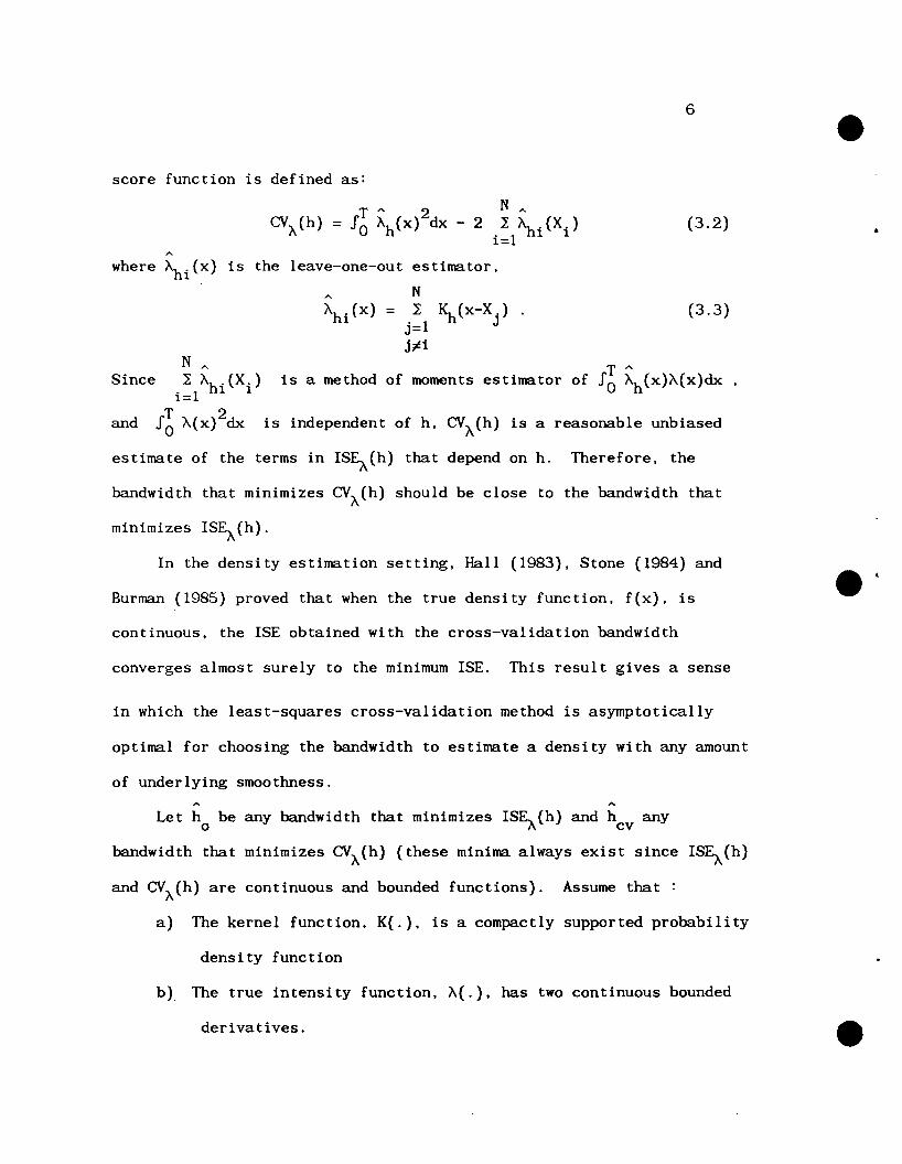
score function is defined as:

(3.2)

'"where Xhi(x) is the leave-one-out estimator.

is independent of h, CVX(h) is a reasonable unbiased

T '"is a method of moments estimator of f O Xh(x)X(x)dx

(3.3)N};

j=1j;l!i

N '"Since }; Xh . (X.)

i=l 1 1

and fb X(x)2dx

estimate of the terms in IS~(h) that depend on h. Therefore, the

bandwidth that minimizes CVX(h) should be close to the bandwidth that

minimizes IS~(h).

In the density estimation setting, Hall (1983). Stone (1984) and

Burman (1985) proved that when the true density function, f(x). is

continuous. the ISE obtained with the cross-validation bandwidth

converges almost surely to the minimum ISE. This result gives a sense

in which the least-squares cross-validation method is asymptotically

optimal for choosing the bandwidth to estimate a density with any amount

of underlying smoothness.

Let ho be any bandwidth that minimizes IS~(h) and hcv any

bandwidth that minimizes CVX(h) (these minima always exist since IS~(h)

and CVX(h) are continuous and bounded functions). Assume that:

a) The kernel function. K(.). is a compactly supported probability

density function

b) The true intensity function. X(.). has two continuous bounded

derivatives.

c)

7

The bandwidths under consideration come from a set H wherec

for each c. -0sup h ~ chcH

c

. f h < (-1+0)In _ c .hcH

c

and

#(Hc ) = {the number of elements in Hc } ~ c P for some

constants 0)0 and p)O. (under the stationary Cox process

model. substitute "J.l" for "c" in this assumption).

Assumption b) is a common technical assumption which allows Taylor

eXPansion methods to be used for studying the error functions of ~h(x).

With assumption c). the set of possible bandwidths nearly covers the

range of consistent bandwidths. Under these assumptions. the

least-squares cross-validation bandwidth is asymptotically optimal for

kernel intensity estimation. This result is stated in Theorem 1.

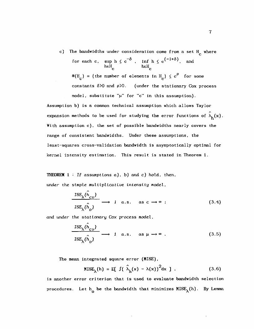
THEOREM 1 : If assumptions a), b) and c) hoLd. then.

under the simpLe muLtipLicative intensity modeL.

ISF_ (h )-" cv

-+ 1 a.s. as c --+ 00 (3.4)

and under the stationary Cox process modeL,

'"ISF- (h )

" cv-+ 1 a.s. as J.l --+ 00 • (3.5)

The mean integrated square error (MISE).

MIS~(h) = E[ J( ~(x) - ~(x))2dx ] (3.6)

is another error criterion that is used to evaluate bandwidth selection

procedures. Let ho

be the bandwidth that minimizes MIS~(h). By Lemma

8

1 in Section 4, the ISE and MISE are essentially the same for large c or

IJ.. As a result of Theorem 1, h is also asymptotically optimal withcv

respect to MISE in the sense that

MISF_ (h )-A. cv--+ 1 a.s. as c --+ 00 or IJ. --+ 00 • (3.7)

In order to prove Theorem 1. we use arguments similar to the

martingale methods employed by HardIe, Marron and Wand (1990) to prove

the asymptotic optimality of density derivatives. In addition. a

martingale inequality given by Burkholder (1973) is used several times.

Details of the proof are presented in Section 4.

4. Proof of Theorem 1

In this section, we outline the proof of Theorem 1. First consider

the simple multiplicative intensity model. That is. the underlying

a(x). and the kernel intensity estimateintensity

is Xh(x)

function is X (x) = cc

N= ~ ~(x-Xi) where E[N]=c.

i=1Assume that assumptions a). b)

and c) hold.

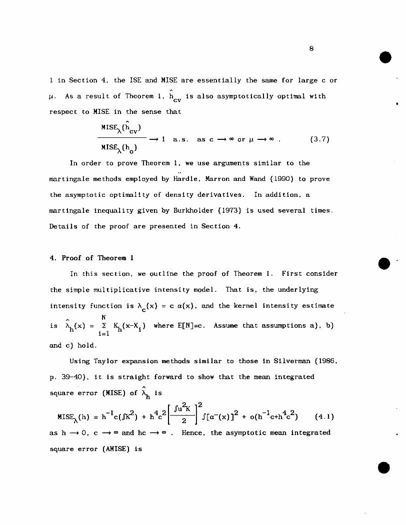
Using Taylor eXPansion methods similar to those in Silverman (1986.

p. 39-40), it is straight forward to show that the mean integrated

square error (MISE) of ~ is

MlSE?-(h) = h-lc(~) + h4C

2 [ IU; rf[un (X)]2 -1 4 2+ o(h c+h c ) (4.1)

as h --+ O. c --+ 00 and hc --+ 00. Hence. the asymptotic mean integrated

square error (AMISE) is

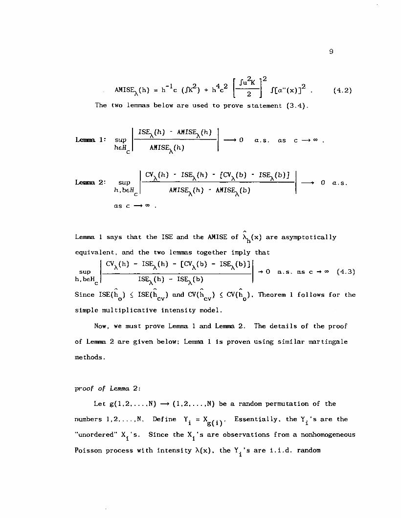
9

(4.2)

The two lemmas below are used to prove statement (3.4).

Lemma 1: suphE:.H

c

IS~(h) - AMIS~(h)

AMIS~(h)

---+ 0 a.s. as c --+ (X) •

Lemma 2: suph,bE:.H

c

CVX(h) - IS~(h) - [CVX(b) - IS~(b)]

AMIS~(h) - AMIS~(b)

---+ 0 a.s.

as c --+ (X)

'"Lemma 1 says that the ISE and the AMISE of ~(x) are asymptotically

equivalent, and the two lemmas together imply that

suph.bE:.H

c

CVX(h) - ISEx(h) - [CVX(b) - ISEx(b)]

ISEx(h) - ISEx(b)-+ 0 a. s. as c -+ (X) (4.3)

'" '"Since ISE(h ) ~ ISE(h ) and CV(h ) < CV(h ). Theorem 1 follows for theo cv cv - 0

simple multiplicative intensity model.

Now, we must prove Lemma 1 and Lemma 2. The details of the proof

of Lemma 2 are given below; Lemma 1 is proven using similar martingale

methods.

proof of Lemma 2:

Let g(I.2 ..... N) --+ (1.2 ..... N) be a random permutation of the

numbers 1.2, ... ,N. Define Y. =X (.). Essentially. the Y.·s are the1 gIl

"unordered" X. ·s. Since the X. 's are observations from a nonhomogeneous1 1

Poisson process with intensity X(x). the Y.·s are i.i.d. random1

10

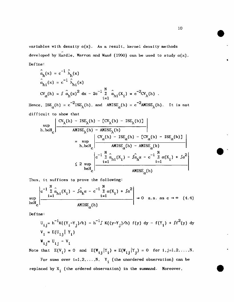
variables with density a(x). As a result. kernel density methods

developed by HardIe. Marron and Wand (1990) can be used to study a(x).

Define:A -1 A

~(x) = c ~h(X)

A -1 A

~i(X) = c ~hi(X)

A 2 -1 N A -2CVa(h) = f ~(x) dx - 2c i:1 ~i(Xi) = c CV~(h) .

-2 -2Hence. ISEa(h) = c IS~(h). and AMISEa(h) = c AMIS~(h). It is not

difficult to show that

AMISE (h)a

~ 2 suphcH

c

= suph.bcH

c

CV~(h) - IS~(h) - [CV~(b) - IS~(b)]

AMIS~ (h) - AMIS~ (b)

CVa(h) - ISEa(h) - [CVa(b) - ISEa(b)]

AMISEa(h) - AMISEa(b)

-1 N A A -1 N 2c ~ ~.(X.) - f~a - c ~ a(X.) + fa

i=1 1 1 i=1 1

suph.bcH

c

Thus. it suffices to prove the following:

-1 N A A -1 N 2c ~ ~.(X.) - f~a - c ~ a(X.) + fa

i=1 1 1 i=1 1suphcHc AMISE (h)

a

~ 0 a.s. as c ~ 00 (4.4)

Define:

U..= h-1K«Y.-Y.)/h) - h-1f K«y-YJ.)/h) fey) dy - f(Y1.) + ff2(y) dy

IJ 1 J

Vi = E(Uijl Yi )

w..= U.. - V.IJ IJ 1

Note that E(V.) = 0 and E(w.jIY.) = E{w.jIY.) = 0 for i.j=1.2 ..... N.III 1 J

For sums over i=1.2 ..... N. Y. (the unordered observation) can be1

replaced by X. (the ordered observation) in the summand. Moreover.1

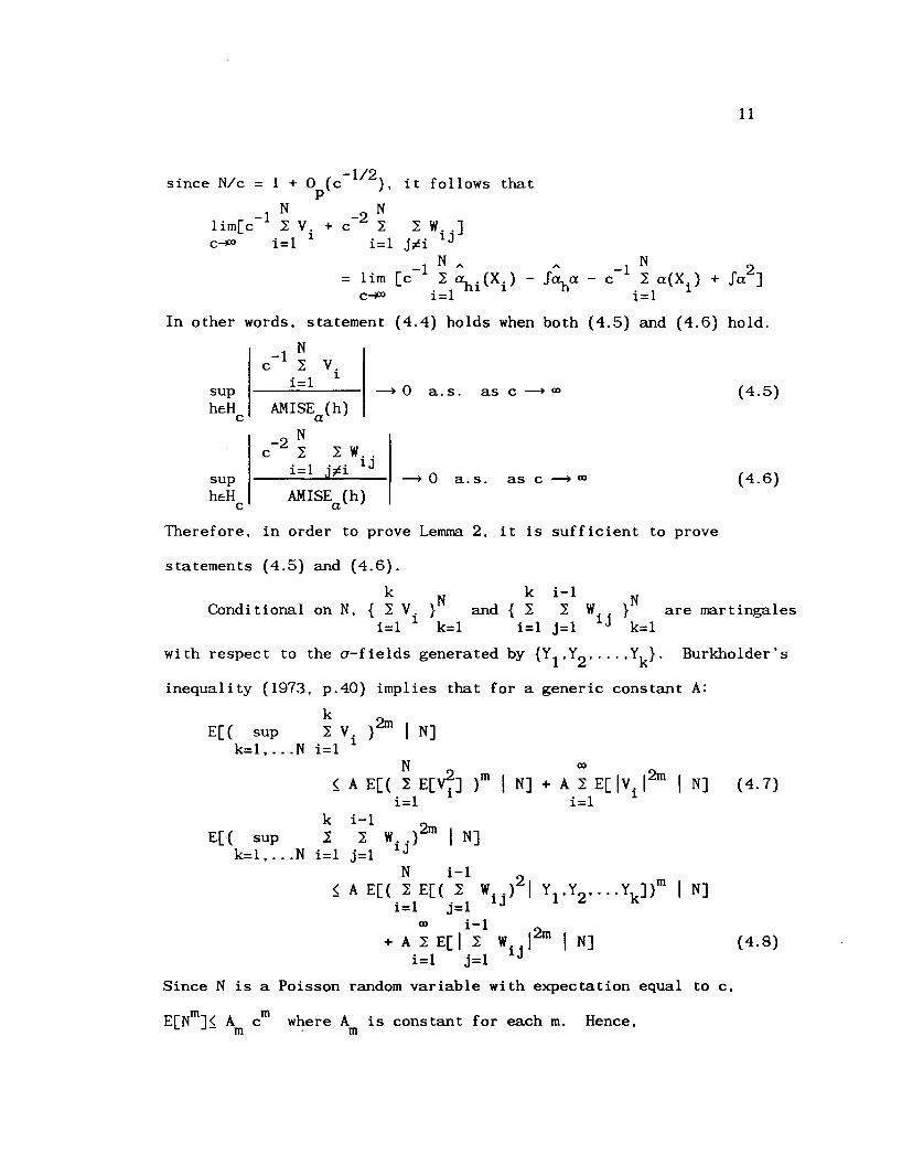
11

-1/2since N/c = 1 + 0 (c ), it follows thatp

-1 N -2 N1im[ c }; V. + C }; }; W.. ]c~ i=1 1 i=1 jti 1J

-1 N A A

= lim [c }; ~.(X.) - f~a -c~ i=1 1 1

-1 N 2c }; a(X.) + fa ]

i=1 1

(4.5)

(4.6)-+ 0 a. s . as c -+ CXl

-+ 0 a. s . as c -+ CXl

AMISEa(h)

-2 Nc }; };W ..

i=1 jti 1JsuphcH

c

suphcH

c

In other words. statement (4.4) holds when both (4.5) and (4.6) hold.

-1 Nc }; V.

i=1 1

Therefore, in order to prove Lemma 2, it is sufficient to prove

statements (4.5) and (4.6).

kConditional on N. { }; V.

i=1 1

k i-I Nand {}; }; W.• } are martingales

i=1 j=1 1J k=1

with respect to the a-fields generated by {Y1

,Y2.· ... Yk}. Burkholder's

inequality (1973. p.40) implies that for a generic constant A:

CXl

+ A }; E[ IV. 12m

I N]i=1 1

E[( supk=l, ... N

E[( supk=l, ... N

k};V.)2m IN]

i=1 1N

~ A E[( }; E[~] )m I N]i=1 1

k i-I}; }; W•• )2m I N]

. 1 . 1 1J1= J=N i-I 2

1m

~ A E[(.}; E[(.}; Wi') Y1.Y2.···Yk])1=1 J=1 J

CXl i-I+ A }; E[ I}; W•• 12m I N]

. 1 . 1 1J1= J=

I N]

(4.7)

(4.8)

Since N is a Poisson random variable with expectation equal to c.

where A is constant for each m.. m Hence.

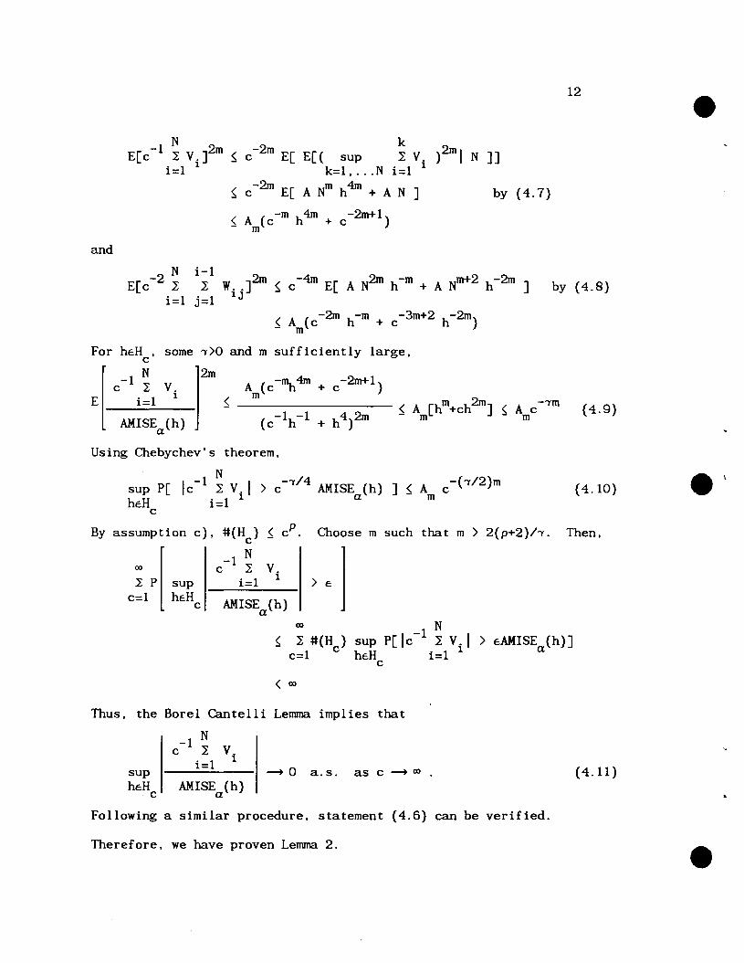
12

. -1 N 2m -2m k 2mE[c ~ V.] ~ c E[ E[( sup ~ V.) IN]]

i=1 1 k=1 .... N i=1 1

~ c-2m E[ A Nm h4m + AN] by (4.7)

~ Am(c-m h4m + c-2m+1)

and

2m

For hcH . some ~>O and m sufficiently large.c

[

c -1 ~ V.

E AM::~ (:)a

(4.9)

Using Chebychev's theorem.

Nsup P[ Ic-1 ~ V. I > c-~/4 AMISE (h) ] ~ A c-(~/2)mhcH i=l 1 a m

c

( 4.10)

By assumption

> cAMISE (h)]a

Then.Choose m such that m > 2(p+2)/~.

AMISE (h)a00 N

~ ~ #(Hc ) sup p[lc-1 ~ viic=1 hcH i=1c

c). #(Hc )

-1 Nc ~ V.

i=1 1suphcH

c

00

~ Pc=1

< 00

(4.11)--+ 0 a. s . as c --+ 00 •suphcH AMISE (h)

c a

Thus. the Borel Cantelli Lemma implies that

-1 Nc ~ Vi

i=1

Following a similar procedure. statement (4.6) can be verified.

Therefore. we have proven Lemma 2.

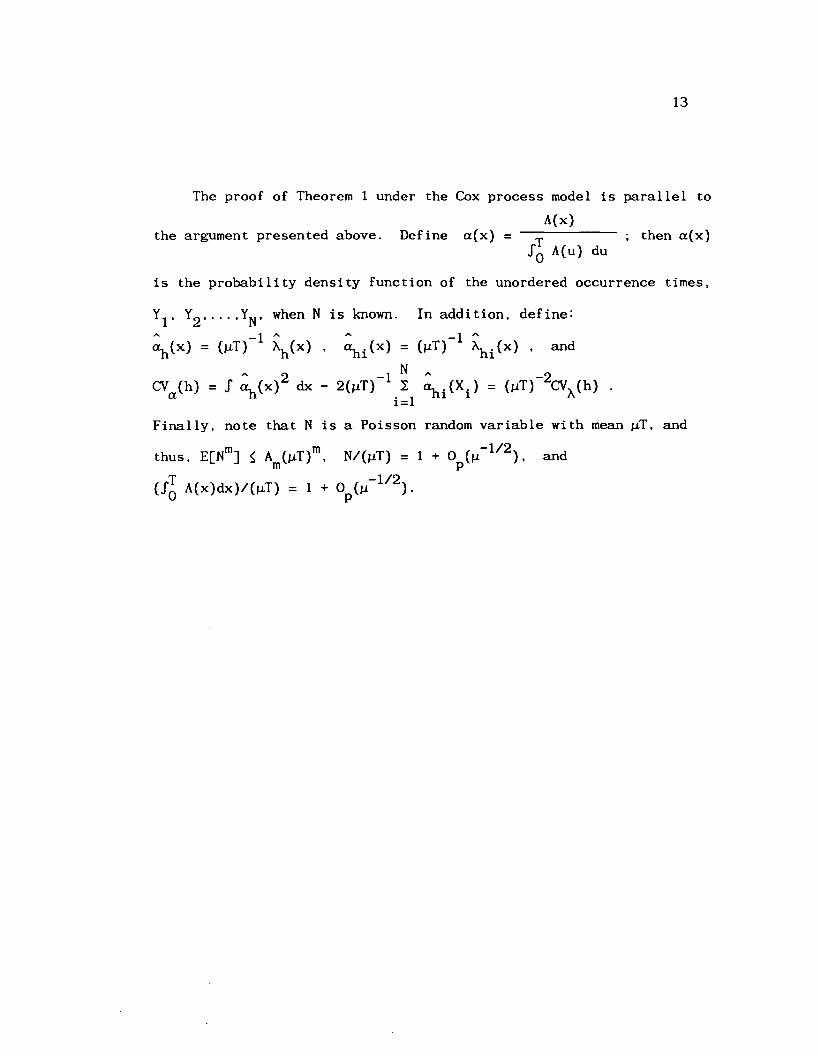
13

The proof of Theorem 1 under the Cox process model is parallel to

the argument presented above. Define a(x) =A(x)

TSo A(u) duthen a(x)

is the probability density function of the unordered occurrence times,

-1 A

(MT) ~hi(x), and

A -2~i(Xi) = (MT) CV~(h)

Y1, Y2 ,·· .,YN, when N is known.A -1 A A

~(x) = (MT) ~h(x), ~i(x) =A 2 1 N

CVa(h) = S ~(x) dx - 2(MT)- Li=1

In addition, define:

Finally, note that N is a Poisson random variable with mean MT, and

m mthus, E[N ] ~ Am(MT), N/(MT) = 1

T -1/2(SO A(x)dx)/(MT) = 1 + 0p(M ).

and

REFERENCES

[1] Aalen. Odd (1978). "Nonparametric Inference for a Family of

Counting Processes." The Annals of Statistics. 6. 701-726.

[2] Andersen, Per Kragh and Borgan. Ornulf (1985), Counting Process

Models for Life History Data: A Review." Scandinavian Journal of

Statistics, 12. 97-158.

[3] Bowman, Adrian W. (1984). "An Alternative of Cross-Validation for

the Smoothing of Density Estimates," Biometrika. 71, 363-60.

[4] Burkholder. D. L. (1973), "Distribution Function Inequal i ties for

Martingales," The Annals of Probability. 1, 19-42.

[5] Burman. Prabir (1985), "A Data Dependent Approach to Density

Estimation," Zei tschrift fur Wahrscheinlichkei tstheorie und

Verwandte Gebiete, 69. 609-628.

[6] Cox, D. R. and Isham. Valerie (1980). Point Processes. Chapman and

Hall, London.

[7] Devroye. Luc and Gyorfi, Laszlo (1984). Nonparametric Density

Estimation: The L1 View. John Wiley and Sons. New York.

[8] Diggle. Peter J. (1983). Statistical Analysis of Spacial Point

Patterns. Academic Press. London.

[9] Diggle. Peter (1985). "A Kernel Method for Smoothing Point Process

Data," Applied Statistics, 34. 138-147.

[10] Diggle. Peter and Marron. J. S. (1988). "EqUivalence of Smoothing

Parameter Selectors in Density and Intensity Estimation." Journal

of the American Statistical Association. 83. 793-800.

"[11] HardIe. Wolfgang. Marron. J. S. and Wand. M. P. (1990). "Bandwidth

Choice for Density Derivatives." to appear in Journal of the Royal

Statistical Society. Series B.

[12J Hall, Peter (1983), "Large Sample Optimality of Least Squares

Cross-Validation in Density Estimation," The Annals of Statistics,

11, 1156-1174.

[13J Leadbetter. M. R. and Wold, Diane (1983), "On Estimation of Point

Process Intensities," Contributions to Statistics: Essays in Honour

of Norman L. Johnson (P.K. Sen. ed.). North-Holland, Amsterdam,

299-312.

[14J Marron. James Stephen and HardIe. Wolfgang (1986), "Random

Approximations to Some Measures of Accuracy in Nonparametric Curve

Estimation," Journal of Multivariate Analysis, 20, 91-113.

[15J Ramlau-Hansen. Henrik (1983a). "Smoothing Counting Process

Intensities by Means of Kernel Functions," The Annals of

Statistics. 11, 453-466.

[16J Ramlau-Hansen. Henrik (l983b), "The Choice of a Kernel Function in

the Graduation of Counting Process Intensities," Scandinavian

Actuarial Journal. 165-182.

[17J Ripley, B. D. (1981). Spatial Statistics. John Wiley and Sons. New

York.

[18J Rosenblatt, Murray (1956) , "Remarks on Some Nonparametric Estimates

of a Density Function. The Annals of Mathematical Statistics," 27.

832-837.

[19J Rosenblatt. Murray (1971). "Curve Estimates." The Annals of

Ma thematical Stat i s tics." 42. 1815-1842.

[20J Rudemo. Mats (1982). "Empirical Choice of Histograms and Kernel

Density Estimators." Scandinavian Journal of Statistics. 9. 65-78.

[21J Silverman, B. W. (1986), Density Estimation for Statistics and Data

Analysis, Chapman and Hall, New York.

[22J Stone, Charles (1984), "An Asymptotically Optimal Window Selection

Rule For Kernel Density Estimates," The Annals of Statistics, 12,

1285-97.