Error estimates for moving least squareapproximationsMar��a G. Armentano� and Ricardo G. Dur�an �AbstractIn this paper we obtain error estimates for moving least square approximations in theone dimensional case. For the application of this method to the numerical solution ofdi�erential equations it is fundamental to have error estimates for the approximations ofderivatives. We prove that, under appropriate hypothesis on the weight function and thedistribution of points, the method produces optimal order approximations of the functionand its �rst and second derivatives. As a consequence, we obtain optimal order errorestimates for Galerkin approximations of coercive problems. Finally, as an application ofthe moving least square method we consider a convection-di�usion equation and proposea way of introducing up-wind by means of a non-symmetric weight function. We presentseveral numerical results showing the good behavior of the method.Key words. error estimates, moving least square, Galerkin approximations, convection-di�usion.AMS Subject Classi�cation. 65L70, 65L10, 65D10.1 IntroductionThe moving least square (MLS) as approximation method has been introduced by Shep-ard [12] in the lowest order case and generalized to higher degree by Lancaster and Salkauskas[6]. The object of those works was to provide an alternative to classic interpolation useful toapproximate a function from its values given at irregularly spaced points by using weightedleast square approximations. However, those papers do not attempt to present an approx-imation theory. More recently, the moving least square method for the numerical solutionof di�erential equations has been considered in several papers, especially in the engineeringliterature, ( [13], [1], [2]) giving rise to a particular class of the so called mesh-less methods�Departamento de Matem�atica, Facultad de Ciencias Exactas y Naturales, 1428 Buenos Aires, Argentina(garmenta@dm.uba.ar, rduran@dm.uba.ar). Supported by Universidad de Buenos Aires under grant TX048and ANPCyT under grant PICT 03-00000-00137. The second author is a member of CONICET, Argentina.1

which provide numerical approximations starting from a set of points instead of a mesh ortriangulation.For this kind of application it is fundamental to analyze the order of approximation, notonly for the function itself, but also for its derivates.We will show that, for the approximation in L1 of the function, optimal error estimates inthe one dimensional case follows from known results concerning the interpolation propertiesof best approximations ([9],[8],[10]) under rather general hypothesis. Also, in a recent paperLevin [7] analyzed the MLS method for a particular weight function obtaining error estimatesin the uniform norm for the approximation of a regular function in higher dimensions.The main object of this work is to prove error estimates for the approximation of the�rst and second order derivatives of a function by the moving least square method in theone dimensional case. We use compact support weight functions as is usually done in theapplication for numerical solution of di�erential equations. In order to obtain these estimateswe will need to impose more restrictive assumptions on the set of points and on the weightfunction used.Our results can be applied in two ways for the approximation to second order problems.The MLS method can be used to construct �nite dimensional approximation spaces to de�neGalerkin approximations. In this case, our results for the �rst derivatives provide optimalorder error estimates by using standard arguments (i.e the Cea' s Lemma ). On the otherhand, the error estimates for the second derivatives allows to control the consistency error of�nite di�erence or collocation methods obtained from an arbitrary set of points by the MLSmethod.One of the most interesting features of the MLS method is the possibility of constructingapproximation spaces which take into account special properties of the di�erential equationconsidered. As an example of this fact we consider a convection-di�usion equation and showhow the MLS method, with a particular weight function, can be used to construct nonsymmetric approximation functions introducing appropriate up-wind.We present numerical computations showing the good behavior of this approach (althoughwe remark that we do not attempt here to provide a theoretical analysis for the convectiondominated problem, i.e, to obtain error estimates valid uniformly on the relation betweenconvection and di�usion. This is an interesting problem and will be the object of our futureresearch).Some of the techniques introduced here for the error analysis can be extended to higherdimensions although this is not trivial and will be presented elsewhere.The paper is organized as follows. First, in Section 2 we present the moving least squaremethod. Section 3 deals with the error estimates for the function and its �rst and secondderivatives. Finally, in Section 4 we use the error estimates to prove the convergence ofGalerkin approximations based on MLS method for second order coercive problem and weconclude with some numerical examples for a convection-di�usion equation.2

2 The Moving Least Square MethodGiven R > 0 let �R � 0 be a function such that supp �R � BR(0) = fz=jzj � Rg.and XR = fx1; x2; : : : ; xng, n = n(R), a set of points in � IR an open interval and letu1; u2; : : :un be the values of the function u in those points, i.e, uj = u(xj), 1 � j � n.Let fp0; � � � ; pmg be a basis of the Polynomial Space Pm. (we can choose, for examplep0 = 1; p1 = x; : : : ; pm = xm) with m << n.For each x 2 (�x) we consider P �(x; y) = Pmk=0 pk(y)�k(x) where f�0(x); � � � ; �m(x)g arechosen such that Jx(�) = nXj=1�R(x� xj)(uj � mXk=0 pk(xj)�k)2 ;is minimized.In order to simplify notation we will drop the subscript R from the weight function �R.Then, we de�ne the approximation of u asu(x) = P �(x; x) = mXk=0 pk(x)�k(x) : (2.1)In order to have this approximation well de�ned we need to guarantee that the minimizationproblem has a solution.We de�ne < f; g >x= nXj=1�(x� xj)f(xj)g(xj) :Then, kfk2x = nXj=1�(x� xj)f(xj)2;is a discrete norm on the polynomial space Pm if the weight function � satis�es the followingpropertyProperty P: For each x 2 , �(x� xj) > 0 at least for m+ 1 indices j.Therefore (see for example [5])Theorem 2.1 Assume that the weight function satis�es property P. Then, for any x 2 there exists P �(x; �) 2 Pm which satis�es ku� P �(x; :)kx � ku� Pkx for all P 2 Pm.Observe that the polynomial P �(x; y) can be obtained solving the normal equations for theminimization problem. In fact, if we denote p(x) = (p0(x) � � �pm(x))t,A(x) =Pnk=1 �(x�xk)p(xk)pt(xk) and cj(x) = �(x�xj)p(xj) then, �(x) = (�0(x); � � � ; �m(x))tis the solution of the following systemA(x)�(x) = nXj=1 cj(x)uj :3

So, an easy calculation shows that P �(x; x) may be written asP �(x; x) = nXj=1 �j(x)uj ; (2.2)where �j(x) = pt(x)A�1(x)cj(x) are functions with the same support and regularity than �([6], section 2). We also note that if u 2 Pk with k � m, then u = u. In particular f�jg1�j�nis a partition of unity, i.e, Pnj=1 �j(x) = 1, 8x 2 . However, the �j are not in general nonnegative functions and this fact make the error analysis more complicated.3 Error EstimatesThe object of this section is to obtain error estimates in terms of the parameter R whichplays the role of the mesh size. The letter C will stand for a constant, independent of R, notnecessarily the same in each occurrence. We will indicate in each case which parameters itdepends on.The approximation order of u to the function u can be obtained from known results onbest least square approximations. Indeed, the following theorem is known (see Theorem 8 in[9])Theorem 3.1 Assume that � satis�es property P. Let x 2 and u 2 Cm+1(BR(x) \ ). IfP �(x; y) is the polynomial in y that minimizes Jx(�), then u(y)� P �(x; y) has at least m+1zeros in BR(x)\ .Therefore, from standard interpolation error estimates we have the followingCorollary 3.1 If � satis�es property P and u 2 Cm+1() then, there exists C, dependingonly on m, such that for each x 2 and any y 2 BR(x)\ ju(y)� P �(x; y)j � Cku(m+1)kL1()Rm+1 ; (3.1)in particular taking y = x, we haveku� ukL1() � Cku(m+1)kL1()Rm+1 : (3.2)For our subsequent error analysis we introduce the following properties about the weightfunction and the distribution of points. All the constants appearing below are independentof R.1. Given x 2 there exist at least m+ 1 points xj 2 XR \BR2 (x).2. 9c0 > 0 such that �(z) � c0 8z 2 BR2 (0).3. � 2 C1(BR(0))\W 1;1(IR) and 9 c1 such that k�0kL1(IR) � c1R .4

4. 9cp such that R� � cp where � = minjxi � xkj is the minimum over the m+ 1 points incondition 1).5. 9c# such that for all x 2 , cardfXR \B2R(x)g < c#.6. � 2 C2(BR(0))\W 2;1(IR) and 9 c2 such that k�00kL1(IR) � c2R2 .Our next goal is to estimate the error in the approximation of u0 by u0. The following Lemmagives the fundamental tool to obtain this estimate.Lemma 3.1 Let x 2 such that @P �(x;y)@x exists and u 2 Cm+1(). If properties 1) to 5)hold then, there exists C = C(c0; c1; cp; c#; m) such that 8y 2 BR(x)\ :j@P �(x; y)@x j � CRmku(m+1)kL1() (3.3)Proof. Given x 2 , in view of property 1) there exist points xj1 ; xj2 ; � � � ; xjm+1 2 BR2 (x).For any h > 0 we de�ne S(x) = Xk2fjig jP �(x+ h; xk)� P �(x; xk)j2 (3.4)Then, by property 2)S(x) � 1c0 Xk2fjig�(x� xk)(P �(x+ h; xk)� P �(x; xk))2� 1c0 nXk=1�(x� xk)(P �(x+ h; xk)� P �(x; xk))2 (3.5)= 1c0 nXk=1�(x� xk)(P �(x+ h; xk)� P �(x; xk))(P �(x+ h; xk)� u(xk))+ 1c0 nXk=1�(x� xk)(P �(x+ h; xk)� P �(x; xk))(u(xk)� P �(x; xk)) :Let Q be the polynomial of degree � m de�ned by Q(y) = P �(x+h; y)�P �(x; y), then sincethe minimum is attained at P � we have< u(y)� P �(x; y); Q(y)>x= nXk=1�(x� xk)Q(xk)(u(xk)� P �(x; xk)) = 0 : (3.6)Then, S(x) � 1c0 nXk=1�(x� xk)Q(xk)(P �(x+ h; xk)� u(xk)) : (3.7)5

Since � is in C1(BR(0))\W 1;1(IR), for h small enough, 9�k such that �(x� xk) = �(x+h� xk)� �0(�k)h and so, replacing in (3.7) we obtainS(x) � 1c0 nXk=1�(x+ h� xk)Q(xk)(P �(x+ h; xk)� u(xk))� hc0 nXk=1�0(�k)Q(xk)(P �(x+ h; xk)� u(xk)) :Since < u(y)�P �(x+h; y); Q(y)>x+h= 0 and using that �0 has compact support togetherwith property 3) we haveS(x) � hc0 nXk=1�0(�k)Q(xk)(u(xk)� P �(x+ h; xk))� hc0 nXk=1 j�0(�k)jjQ(xk)jj(P �(x+ h; xk)� u(xk))j� c1hc0R Xxk2B2R(x) jQ(xk)jj(P �(x+ h; xk)� u(xk))j :By Corollary 3.1 we know that jP �(x+ h; xk)� u(xk)j � Cku(m+1)kL1()Rm+1 then,S(x) � Chku(m+1)kL1()Rm Xxk2B2R(x) jQ(xk)j (3.8)Since Q is a polynomial of degree � m it can be written asQ(y) = Xk2fjigQ(xk)lk(y) ; (3.9)where lk(y) are the Lagrange's polynomial basis functions and thereforeXxk2B2R(x) jQ(xk)j � Xi2fjkg jQ(xi)j( Xxk2B2R(x) jli(xk)j)From property 4) jli(y)j � (2R� )m+1 � c(cp; m) 8i 2 fjk; 1 � k � m + 1g and therefore, itfollows from property 5) and (3.8) that( Xk2fjig jQ(xk)j)2 � (m+ 1) Xk2fjig jQ(xk)j2 = (m+ 1)S(x) (3.10)� Chku(m+1)kL1()Rmc# Xk2fjig jQ(xk)jNow, we obtain Xk2fjig jQ(xk)j � Chku(m+1)kL1()Rm : (3.11)6

Finally, using (3.11) and property 4) in (3.9) we get 8y 2 BR(x)\ jQ(y)jh = jP �(x+ h; y)� P �(x; y)jh � Cku(m+1)kL1()Rm ; (3.12)and so, if x is a point such that @P �(x;y)@x exists, the proof concludes by taking h! 0.The following Theorem states the order which u0 approximates u0.Theorem 3.2 If u 2 Cm+1() and properties 1) to 5) hold then, there exists C = C(c0; c1; cp; c#; m)such that ku0 � u0kL1() � Cku(m+1)kL1()Rm : (3.13)Proof. Observe that, since � 2 C1(BR(0)) \ W 1;1(IR) then, P �(x; y) is continuous every-where and di�erentiable for every x up to a �nite set (this can be seen using again theargument given in [6], section 2). Therefore, P �(�; y) 2 W 1;1(). For any x 2 such that@P �(x;y)@x exists, we want to estimate ju0(x)� u0(x)j = ju0(x)� ddxP �(x; x)j. We note thatddxP �(x; x) = f@P �(x; y)@x + @P �(x; y)@y @y@xgjy=x (3.14)So, we will estimate ju0(y) � @P �(x;y)@x � @P �(x;y)@y j, 8y 2 BR(x) \ . Since P �(x; y) is apolynomial of degree � m that interpolates u at m+ 1 points (Theorem 3.1) then, @P �(x;y)@yinterpolates u0 in m points and therefore,ju0(y)� @P �(x; y)@y j � Cku(m+1)kL1()Rm 8y 2 BR(x) \ (3.15)From Lemma 3.1 we know that j@P �(x;y)@x j � Cku(m+1)kL1()Rm which together with (3.15)yieldsju0(y)� @P �(x; y)@x � @P �(x; y)@y j � ju0(y)� @P �(x; y)@y j+ j@P �(x; y)@x j � Cku(m+1)kL1()RmIn particular taking y = x we conclude the proof.Our next goal is to �nd error estimates for the approximation of u00 by u00. The idea ofthe proof is similar to that used for the �rst derivative. However, instead of using the orthog-onality (3.6) we have to use a relation which is obtained in the next lemma by di�erentiatingit. From now on we will assume that � 2 C1(IR) so, in particular P �(�; y) 2 C1() using thesame argument mentioned above.Lemma 3.2 For any Q(x; y) polynomial in y of degree � m and di�erentiable as a functionof x we havenXj=1�0(x� xj)Q(x; xj)(P �(x; xj)� uj) + nXj=1�(x� xj)Q(x; xj)@P �(x; xj)@x = 0 : (3.16)7

Proof. Since P �(x; y) is the minimum, for each x 2 ,< u(y)� P �(x; y); Q(x; y)>x= 0 8 Q(x; �) 2 Pm (3.17)then if we take derivative with respect to x we havenXj=1�0(x� xj)Q(x; xj)(P �(x; xj)� uj) + nXj=1�(x� xj)@Q(x; xj)@x (P �(x; xj)� uj)+ nXj=1�(x� xj)Q(x; xj)@P �(x; xj)@x = 0 :Since for each x, @Q(x;y)@x is in Pm and P � satis�es (3.17) the second term is 0 and thereforewe have the result.Proceeding as we have done for the error in the �rst derivative we will need to estimatethe second derivatives @2P �(x;y)@x2 and @2P �(x;y)@x@y for each x 2 where they exist. This is donein the two following Lemmas.Lemma 3.3 Let x 2 such that @2P �(x;y)@x2 exists , m � 1 and u 2 Cm+1(). If properties 1)to 6) hold then, there exists C = C(c0; c1; c2; cp; c#; m) such that 8y 2 BR(x)\ j@2P �(x; y)@x2 j � CRm�1ku(m+1)kL1() (3.18)Proof. Let x 2 and xj1 ; xj2; � � � ; xjm+1 be as in the proof of Lemma 3.1. Let h > 0 andQ 2 Pm be de�ned by Q(y) = @P �(x+ h; y)@x � @P �(x; y)@x andS(x) = Xk2fjig jQ(xj)j2 : (3.19)From property 2) we haveS(x) � 1c0 Xk2fjig�(x� xk)Q(xk)2 � 1c0 nXk=1�(x� xk)Q(xk)2= 1c0f nXk=1�(x� xk)Q(xk)@P �(x+ h; xk)@x � nXk=1�(x� xk)Q(xk)@P �(x; xk)@x g :(3.20)Now we consider the �rst term on the right hand side of (3.20). Using that for h small enough�(x� xk) = �(x+ h� xk)� h�0(�k) and Lemma 3.2 we havenXk=1�(x� xk)Q(xk)@P �(x+ h; xk)@x = nXk=1�(x+ h� xk)Q(xk)@P �(x+ h; xk)@x� h nXk=1�0(�k)Q(xk)@P �(x+ h; xk)@x= nXk=1�0(x+ h� xk)Q(xk)(uk � P �(x+ h; xk))� h nXk=1�0(�k)Q(xk)@P �(x+ h; xk)@x ;8

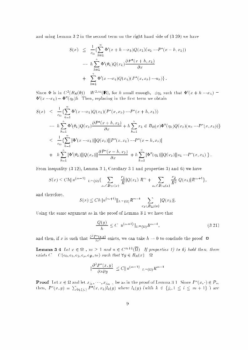
and using Lemma 3.2 in the second term on the right hand side of (3.20) we haveS(x) � 1c0f nXk=1�0(x+ h� xk)Q(xk)(uk � P �(x+ h; xk))� h nXk=1�0(�k)Q(xk)@P �(x+ h; xk)@x+ nXk=1�0(x� xk)Q(xk)(P �(x; xk)� uk)g :Since � is in C2(BR(0)) \W 2;1(IR), for h small enough, 9�k such that �0(x + h � xk) =�0(x� xk) + �00(�k)h. Then, replacing in the �rst term we obtainS(x) � 1c0 f nXk=1�0(x� xk)Q(xk)(P �(x; xk)� P �(x+ h; xk))� h nXk=1�0(�k)Q(xk)@P �(x+ h; xk)@x + h nXk=1 xk 2 BR(x)�00(�k)Q(xk)(uk � P �(x; xk))g� 1c0 f nXk=1 j�0(x� xk)jjQ(xk)jjP �(x; xk)� P �(x+ h; xk)j+ h nXk=1 j�0(�k)jjQ(xk)jj@P �(x+ h; xk)@x j+ h nXk=1 j�00(�k)jjQ(xk)jjuk � P �(x; xk)jg :From inequality (3.12), Lemma 3.1, Corollary 3.1 and properties 3) and 6) we haveS(x) � Chku(m+1)kL1()f Xxk2B2R(x) c1R jQ(xk)jRm + Xxk2B2R(x) c2R2 jQ(xk)jRm+1g;and therefore, S(x) � Chku(m+1)kL1()Rm�1 Xxk2B2R(x) jQ(xk)j:Using the same argument as in the proof of Lemma 3.1 we have thatjQ(y)jh � Cku(m+1)kL1()Rm�1; (3.21)and then, if x is such that @2P �(x;y)@x2 exists, we can take h! 0 to conclude the proof.Lemma 3.4 Let x 2 , m � 1 and u 2 Cm+1(). If properties 1) to 6) hold then, thereexists C = C(c0; c1; c2; cp; c#; m) such that 8y 2 BR(x) \ j@2P �(x; y)@x@y j � Cku(m+1)kL1()Rm�1Proof. Let x 2 and let xj1 ; � � � ; xjm+1 be as in the proof of Lemma 3.1. Since P �(x; �) 2 Pmthen, P �(x; y) = Pk2fjig P �(x; xk)lk(y) where lk(y) (with k 2 fji; 1 � i � m + 1g ) are9

the Lagrange's polynomial basis functions associated with the points xj1 ; � � � ; xjm+1 . Sinceproperty 6) holds P � is C1 in the �rst variable. Therefore, for any x we have@2P �(x; y)@x@y = Xk2fjig @P �(x; xk)@x l0k(y):By Lemma 3.1 we know that 8y 2 BR(x): j@P �(x;y)@x j � Cku(m+1)kL1()Rm . Thenj@2P �(x; y)@x@y j � Xk2fjig j@P �(x; xk)@x jjl0k(y)j � Cku(m+1)kL1()Rm Xk2fjig jl0k(y)j: (3.22)An easy calculation shows that from property 5) it follows that jl0k(y)j � m cm�1p� � c� andusing this estimate in (3.22) and property 5) again we obtain the result .Theorem 3.3 Let m � 1, if u 2 Cm+1() and properties 1) to 6) hold then, there existsC = C(c0; c1; c2; cp; c#; m) such thatku00 � u00kL1() � Cku(m+1)kL1()Rm�1: (3.23)Proof. Since � 2 C2(BR(0)) \ W 2:1(IR) then, @2P �(x;y)@x@y exists everywhere and @2P �(x;y)@x2exists for every x up to a �nite set and P �(�; y) 2 W 2;1(). (this can be seen using againthe argument given in [6] mentioned above).Given any x 2 , such that @2P �(x;y)@x2 exists, we want to estimate ju00(x)� u00(x)j = ju00(x)�d2dx2P �(x; x)j. We note thatd2dx2P �(x; x) = f@2P �(x; y)@x2 + 2@2P �(x; y)@x@y + @2P �(x; y)@y2 gjy=x (3.24)So, 8y 2 BR(x)\ ju00(y)�@2P �(x; y)@y2 �2@2P �(x; y)@x@y �@2P �(x; y)@x2 j � ju00(y)�@2P �(x; y)@y2 j+2j@2P �(x; y)@x@y j+j@2P �(x; y)@x2 j(3.25)Now observe that, @2P �(x;y)@y2 is a polynomial of degree � m�2 which interpolates u00 in m�1points and thereforeju00(y)� @2P �(x; y)@y2 j � Cku(m+1)kL1()Rm�1 8y 2 BR(x)\ (3.26)Then, the proof concludes by taking y = x and using Lemma 3.3, Lemma 3.4 and (3.25).4 Numerical ExamplesThe object of this section is to present some examples on the numerical solution of di�erentialequations by the MLS method. 10

In order to show the di�erent possibilities of this method we apply it to solve theconvection-di�usion equation �u00 + bu0 = 0; in (0; 1) (4.1)u(0) = 0; u(1) = 1with di�erent values of the constant b > 0 and using Galerkin and Collocation methods.One of the interesting features of the MLS methods is the possibility of choosing appropriateweight function for the problem considered. For example, for the equation (4.1) one canchoose � depending on b taking into account the non-symmetric character of the problemand thus, introducing some kind of upwinding when b is large in order to avoid oscillations.In the �rst two examples we use Galerkin approximations. In general, given the followingvariational problem �nd u 2 V � H1() such thata(u; v) = L(v); 8v 2 Vwhere a is a bilinear form, continuous and coercive on V and L is a linear and continuousoperator, we can use the MLS method to de�ne Galerkin approximation in the following way.Let VR = spanf�1; : : : ; �ng, with �j , 1 � j � n the basis functions de�ned in (2.2).Observe that, since the basis �j have the same regularity as �, if � 2 C1(BR(0))\W 1;1(IR)then �j 2 H1() and therefore we can de�ne the Galerkin approximation uR 2 VR asuR(x) = nXj=1 �j(x)uj ;where u1; : : : ; un is the solution of the following systemnXj=1 a(�j ; �k)uj = L(�k); 1 � k � nFrom C�ea's Lemma ([3], [4]), Theorem 3.2 and Theorem 3.3 we have that :ku� uRkV � � minv2Vh ku� vkV � � ku� ukV � Cku(m+1)kL1()Rm (4.2)where is the continuity constant and � is the coercivity constant of a(�; �) on V . In particularwe have that uR converges to u when R! 0.Now, we write the convection-di�usion equation (4.1) in the following equivalent form.Let ~u(x) = u(x)� x then, we have �~u00 + b~u0 = �b (4.3)~u(0) = ~u(1) = 0The variational problem is to �nd ~u 2 V = H10 (0; 1), such that:a(~u; v) = L(v); 8v 2 V11

where a(~u; v) = Z 10 ~u0v0 + Z 10 b~u0vL(v) = � Z 10 bvThe bilinear form a(�:�) is coercive and continuous [11] therefore, the error estimate (4.2)holds (with the constant C depending on b).For R > 0 we take the following weight function�(z) = 8>><>>: e�( zR )2�e�1�e� if �R < z < 0e ( zR )2�e 1�e if 0 � z < R0 otherwise; (4.4)where � and are constants to be chosen in each example. We consider the two cases b = 1and b = 20. In order to compute the integrals involved in the Galerkin approximation weproceed as follows: Since the basis functions are smooth except in a �nite number of points,we divide their supports in a �nite number of intervals and compute each integral using themid point quadrature rule.In the �rst case the convection and the di�usion are of the same order and so, no upwindingis needed. We include this example to check the predicted convergence order. Therefore, wetake � = = 1 to obtain a symmetric weight function (see Figure 1). We show in Figure 2the approximate solution for equally spaced points with n = 5 and m = 1. The Figures 3and 4 show the logarithm of the error in L1 norm as a function of the logarithm of R for thefunction and its �rst derivative respectively. It is observed that optimal order approximationis obtained in L1 both for u and u0. In particular, the predicted order of convergence in H1is obtained.For the case b = 20 the problem becomes convection dominated and so we take a non-symmetric weight function by choosing � = �30 and = 1 (see Figure 5). We show theresults obtained by using standard linear �nite elements, usual up-wind �nite di�erence andMLS for equaly spaced points. Figure 6, 7 and 8 show the results for n=5 and Figure 9,10and 11 for n=10. As it is known, the �rst method produces oscillations. Instead the othertwo methods do not present oscillations but MLS produces a better approximation. Indeed,although we have not proved it, we expect that the MLS method allows to introduce up-windbut preserving the second order convergence when R! 0.Another way of applying the MLS to solve di�erential equations is by using collocation.Observe that, if � 2 C2(IR) then the basis function �j are in C2(). So, taking m = 2 itfollows from Theorem 3.2 and Theorem 3.3 that the collocation method is consistent. Againwe can introduce up-wind by means of a non-symmetric weight function. We modify thefunction (4.4) in order to obtain a C2 function as follows (Figure 12)�(z) = 8>><>>: e�( zR )4�e�1�e� (1� ( zR)2)4 if �R < z < 0e ( zR )4�e 1�e (1� ( zR)2)4 if 0 � z < R0 otherwise;12

where � = �30 and = 1. We show the approximate solution for equally spaced points withn = 8 and n = 15 (Figure 13 and Figure 14). Again we observe that oscillations do notappear.-0.08 -0.06 -0.04 -0.02 0 0.02 0.04 0.06 0.080

0.1

0.2

0.3

0.4

0.5

0.6

0.7

0.8

0.9

1

weight functionFigure 1: Symmetric weight function13

0 0.1 0.2 0.3 0.4 0.5 0.6 0.7 0.8 0.9 10

0.1

0.2

0.3

0.4

0.5

0.6

0.7

0.8

0.9

1

MLS

m = 1 n = 5 b = 1

true solution

approximationFigure 2: Exact solution vs. MLS approximation−3 −2.8 −2.6 −2.4 −2.2 −2 −1.8 −1.6 −1.4 −1.2

−8.5

−8

−7.5

−7

−6.5

−6

−5.5

−5

−4.5

−4

log(R)

log(

Err

or)

Figure 3: ku� uRkL1() = O(R2)14

−3 −2.8 −2.6 −2.4 −2.2 −2 −1.8 −1.6 −1.4 −1.2−4.8

−4.6

−4.4

−4.2

−4

−3.8

−3.6

−3.4

−3.2

−3

log(R)

log(

Err

or)

Figure 4: ku0 � u0RkL1() = O(R)-0.5 -0.4 -0.3 -0.2 -0.1 0 0.1 0.2 0.3 0.4 0.50

0.1

0.2

0.3

0.4

0.5

0.6

0.7

0.8

0.9

1

weight functionFigure 5: Nonsymmetric weight function15

0 0.1 0.2 0.3 0.4 0.5 0.6 0.7 0.8 0.9 1-0.5

0

0.5

1

n= 5 b= 20

finite element

true solutionapproximation

Figure 6: Exact Solution vs. Finite Element approximation0 0.1 0.2 0.3 0.4 0.5 0.6 0.7 0.8 0.9 1

0

0.1

0.2

0.3

0.4

0.5

0.6

0.7

0.8

0.9

1finite difference

n= 5 b= 20

true solution

approximationFigure 7: Exact solution vs. up-wind Finite Di�erence approximation16

0 0.1 0.2 0.3 0.4 0.5 0.6 0.7 0.8 0.9 1-0.2

0

0.2

0.4

0.6

0.8

1

MLS

m = 1 n = 5 b = 20

true solutionapproximationFigure 8: Exact solution vs. MLS approximation

0 0.1 0.2 0.3 0.4 0.5 0.6 0.7 0.8 0.9 1-0.2

0

0.2

0.4

0.6

0.8

1

n= 10 b= 20

finite element

true solutionapproximation

Figure 9: Exact Solution vs. Finite Element approximation17

0 0.1 0.2 0.3 0.4 0.5 0.6 0.7 0.8 0.9 10

0.1

0.2

0.3

0.4

0.5

0.6

0.7

0.8

0.9

1finite difference

n= 10 b= 20

true solution

approximationFigure 10: Exact solution vs. up-wind Finite Di�erence approximation0 0.1 0.2 0.3 0.4 0.5 0.6 0.7 0.8 0.9 1

0

0.1

0.2

0.3

0.4

0.5

0.6

0.7

0.8

0.9

1

MLS

m = 1 n = 10 b = 20

true solution

approximationFigure 11: Exact solution vs. MLS approximation18

-0.4 -0.3 -0.2 -0.1 0 0.1 0.2 0.3 0.40

0.1

0.2

0.3

0.4

0.5

0.6

0.7

0.8

0.9

1

weight functionFigure 12: Smooth weight function0 0.1 0.2 0.3 0.4 0.5 0.6 0.7 0.8 0.9 1

−0.2

0

0.2

0.4

0.6

0.8

1

1.2 m = 2 n = 8 b = 20

true solutionapproximationFigure 13: Exact solution vs. MLS approximation using Collocation19

0 0.1 0.2 0.3 0.4 0.5 0.6 0.7 0.8 0.9 10

0.2

0.4

0.6

0.8

1

1.2

1.4 m = 2 n = 15 b = 20

true solutionapproximationFigure 14: Exact solution vs. MLS approximation using CollocationReferences[1] Belytschko T. Lu Y.Y., Gu L. A new implementation of the element free Galerkinmethod, Comput. Methods Appl. Mech. Engrg., 113, 397-414 (1994).[2] Belytschko T., Krysl P. Element-free Galerkin method: Convergence of the continuousand discontinuous shape functions , Comput. Methods Appl. Mech. Engrg., 148, 257-277(1997).[3] Brenner S. C. and Scott L. R. The Mathematical Theory of Finite Element Methods ,Springer-Verlag, New York, 1994.[4] Ciarlet P. G. The Finite Element Method for Elliptic Problems, North Holland, Ams-terdam, 1978.[5] Johnson L. W., Riess R. D. Numerical Analysis, Addison-Wesley, 1982.[6] Lancaster, P. Salkauskas K. Surfaces Generated by Moving Least Squares Methods, Math-ematics of Computation,37,141-158 1981.[7] Levin, D. The approximation power of moving least-squares, Mathematics ofComputation,67,1335-1754 1998.[8] Marano M. Mejor Aproximaci�on Local , Tesis de Doctorado en Matem�aticas - U. N. deSan Luis, 1986.[9] Motzkin, T. S. and Walsh J. L. Polynomials of best approximation on a real �nite pointset, Trans. Amer. Math. Soc.,91, 231-245 1959.20

[10] Rice, J. R. Best approximation and interpolating functions, Trans. Amer. Math. Soc.,101,477-498 1961.[11] Roos H. G., Stynes M. and Tobiska L. Numerical Methods for Singularity PerturbedDi�erential Equations, Springer, 1996.[12] Shepard D. A two-dimensional interpolation function for irregularly spaced points, Proc.A.C.M Natl. Conf. ,517-524 1968.[13] Taylor R., Zienkiewicz O. C., O~nate E., and Idelsohn S. Moving least square approxi-mations for the solution of di�erential equations, , CIMNE, report'95.

21