1.1. Maps of Lands Close to Sea Level along the Middle Atlantic Coast of the United States: An Elevation Data Set to Use While Waiting for LIDAR

James G. Titus Environmental Protection Agency and Jue Wang Pyramid Systems, Incorporated Revised May 2008 This section should be cited as: Titus J.G., and J. Wang. 2008. Maps of Lands Close to Sea Level along the Middle Atlantic Coast of the United States: An Elevation Data Set to Use While Waiting for LIDAR. Section 1.1 in: Background Documents Supporting Climate Change Science Program Synthesis and Assessment Product 4.1, J.G. Titus and E.M. Strange (eds.). EPA 430R07004. U.S. EPA, Washington, DC.

This report provides a coastal elevation data set for the mid-Atlantic for purposes of assessing the potential for coastal lands to be inundated by rising sea level. Depending on what we were able to obtain, our elevation estimates are based on LIDAR, federal or state spot elevation data, local government topographic information, and USGS 1:24,000 scale topographic maps. We use wetlands and tide data to define a supplemental elevation contour at the upper boundary of tidal wetlands. Unlike most coastal mapping studies, we express elevations relative to spring high water rather than a fixed reference plane, so that the data set measures the magnitude of sea level rise required to tidally flood lands that are currently above the tides. Our study area includes the seven coastal states from New York to North Carolina, plus the District of Columbia. We assess the accuracy of our approach by comparing our elevation estimates with LIDAR from Maryland and North Carolina. The root mean square error at individual locations appears to be approximately one-half the contour interval of the input data. We also compared the cumulative amount of land below particular elevations according to our estimates and the LIDAR; in that context, our error was generally less than one-quarter the contour interval of the input data.

We estimate that the dry land in the region has a relatively uniform elevation distribution within the first 5 meters above the tides, with about 1,200–1,500 km2 for each 50 cm of elevation. With the exception of North Carolina, the area of nontidal wetlands declines gradually from about 250 km2 within 50 cm above the tides to about 150 km2 between 450 and 500 cm above the tides. North Carolina has approximately 3,000 km2 of nontidal wetlands within 1 meter above spring high water; above that elevation, the amount of nontidal wetlands declines gradually as with the other states. North Carolina accounts for more than two-thirds of the dry land and nontidal wetlands within 1 meter above the tides. We also compare our results to previous studies estimating the region's vulnerability to sea level rise. Our results are broadly consistent with an EPA mapping study published in 2001, which estimated the total amount of land below the 1.5- and 3.5-m contours (relative to the National Geodetic Vertical Datum of 1929). This study appears to be a significant downward revision, however, of EPA's 1989 Report to Congress. Our estimates of the dry land vulnerable to a 50- or 100-cm global rise in sea level are less than one-half the estimates of the Report to Congress. The regional estimates of that nationwide study, however, were based on a small sample. Therefore, one should not extrapolate our mid-Atlantic result to conclude that EPA’s previously reported nationwide estimate overstates reality by a similar magnitude.

Abstract

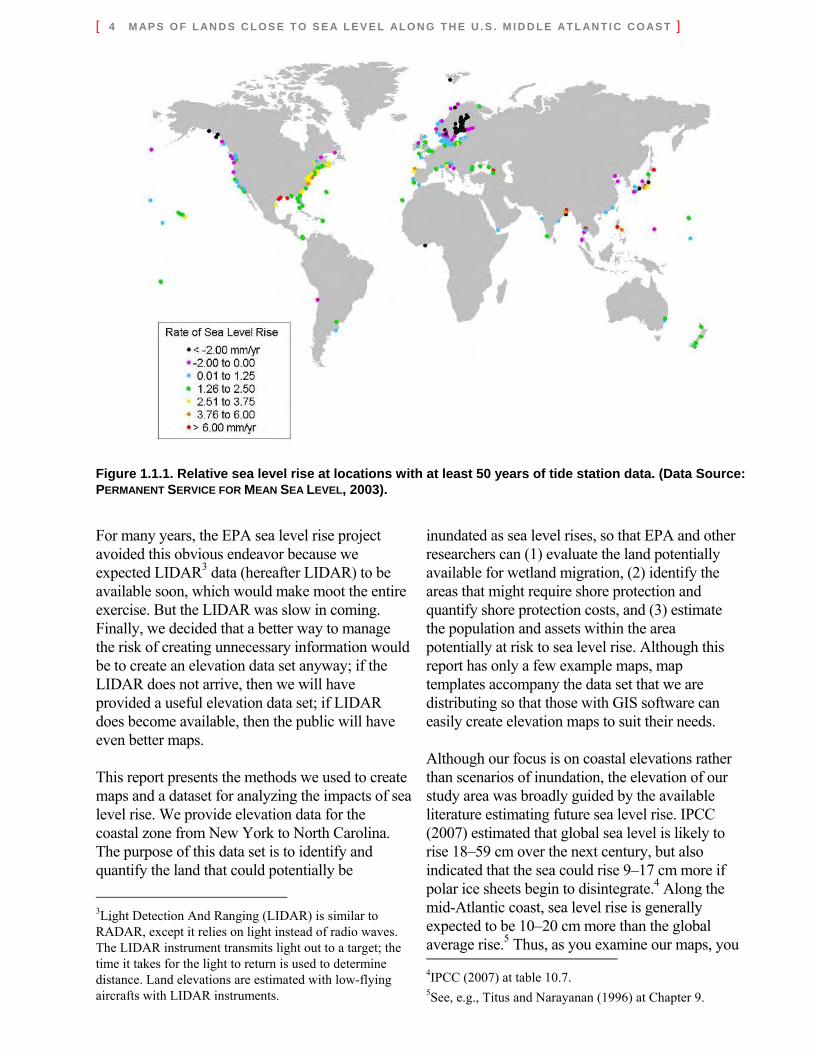
During the last two decades, the issue of rising sea level has spread from being primarily a concern of coastal geologists (e.g., PILKEY et al., 1982) and those who measure the tides (e.g. HICKS et al., 1983; ZERVAS, 2001) to an issue that concerns planners, policymakers, and the public at large (e.g., KRISTOFF, 2005; DEAN 2006). One reason is that the sea is rising 3 mm/yr or more along many low-lying areas (Figure 1.1.1), enough for some areas that were developed 50–100 years ago to be flooded by high tides during new or full moons (Figure 1.1.2). Another reason is that increasing concentrations of carbon dioxide and other greenhouse gases appear to be contributing to a global warming responsible for at least part of the current rate of sea level rise (e.g., U.S. EPA, 1996; IPCC, 2007). Most scientists expect greenhouse gases to accelerate the rise in sea level (IPCC, 2001a), and some have suggested that it may already be doing so (CHURCH and WHITE, 2006). Rising sea level inundates low-lying lands, erodes wetlands and beaches, exacerbates flooding, and increases the salinity of estuaries and aquifers (e.g., IPCC, 2001b). Studies over the last two decades have identified numerous decisions that may be sensitive to sea level rise (e.g., NRC, 1987; WILLIAMS et al., 1995; TITUS and NARAYANAN1, 1996). During the Administration of President George W. Bush, the U.S. Climate

1Section 3.1 of that paper is an overview of decisions that depend on the probability of the sea rising a particular magnitude.

Change Research Program (2003) has actively promoted decision support research to assist with adaptation to consequences of climate changes such as rising sea level. Studies sponsored by the U.S. EPA have suggested that local governments may be making the most important decisions regarding the eventual impact of rising sea level on the United States. Local governments create the land use plans and issue the construction permits that determine whether the areas at risk will be developed enough to require shore protection as the sea rises or will remain vacant enough for wetlands to migrate inland (TITUS, 1990, 1998). Over the last several years, EPA staff and contractors have met with local governments concerning possible responses to sea level rise (TITUS, 2005). When we have asked what information might help them to better prepare, the most common answer has been better elevation maps. When senior government officials or newspaper reporters have asked us about vulnerability to sea level rise, the most common request has been for a map showing the lands that might be flooded. Yet maps depicting lands close to sea level using the best available data are unavailable for most areas.2

2But see WEISS AND OVERPECK (2006), which provides a map server using the USGS national elevation data series.

1.1.1 Introduction

[ 4 M AP S O F L AN D S C L O S E T O S E A L E V E L AL O N G T H E U . S . M I D D L E AT L AN T I C C O AS T ]

For many years, the EPA sea level rise project avoided this obvious endeavor because we expected LIDAR3 data (hereafter LIDAR) to be available soon, which would make moot the entire exercise. But the LIDAR was slow in coming. Finally, we decided that a better way to manage the risk of creating unnecessary information would be to create an elevation data set anyway; if the LIDAR does not arrive, then we will have provided a useful elevation data set; if LIDAR does become available, then the public will have even better maps. This report presents the methods we used to create maps and a dataset for analyzing the impacts of sea level rise. We provide elevation data for the coastal zone from New York to North Carolina. The purpose of this data set is to identify and quantify the land that could potentially be

3Light Detection And Ranging (LIDAR) is similar to RADAR, except it relies on light instead of radio waves. The LIDAR instrument transmits light out to a target; the time it takes for the light to return is used to determine distance. Land elevations are estimated with low-flying aircrafts with LIDAR instruments.

inundated as sea level rises, so that EPA and other researchers can (1) evaluate the land potentially available for wetland migration, (2) identify the areas that might require shore protection and quantify shore protection costs, and (3) estimate the population and assets within the area potentially at risk to sea level rise. Although this report has only a few example maps, map templates accompany the data set that we are distributing so that those with GIS software can easily create elevation maps to suit their needs. Although our focus is on coastal elevations rather than scenarios of inundation, the elevation of our study area was broadly guided by the available literature estimating future sea level rise. IPCC (2007) estimated that global sea level is likely to rise 18–59 cm over the next century, but also indicated that the sea could rise 9–17 cm more if polar ice sheets begin to disintegrate.4 Along the mid-Atlantic coast, sea level rise is generally expected to be 10–20 cm more than the global average rise.5 Thus, as you examine our maps, you 4IPCC (2007) at table 10.7. 5See, e.g., Titus and Narayanan (1996) at Chapter 9.

Figure 1.1.1. Relative sea level rise at locations with at least 50 years of tide station data. (Data Source: PERMANENT SERVICE FOR MEAN SEA LEVEL, 2003).

[ S E C T I O N 1 . 1 5 ]

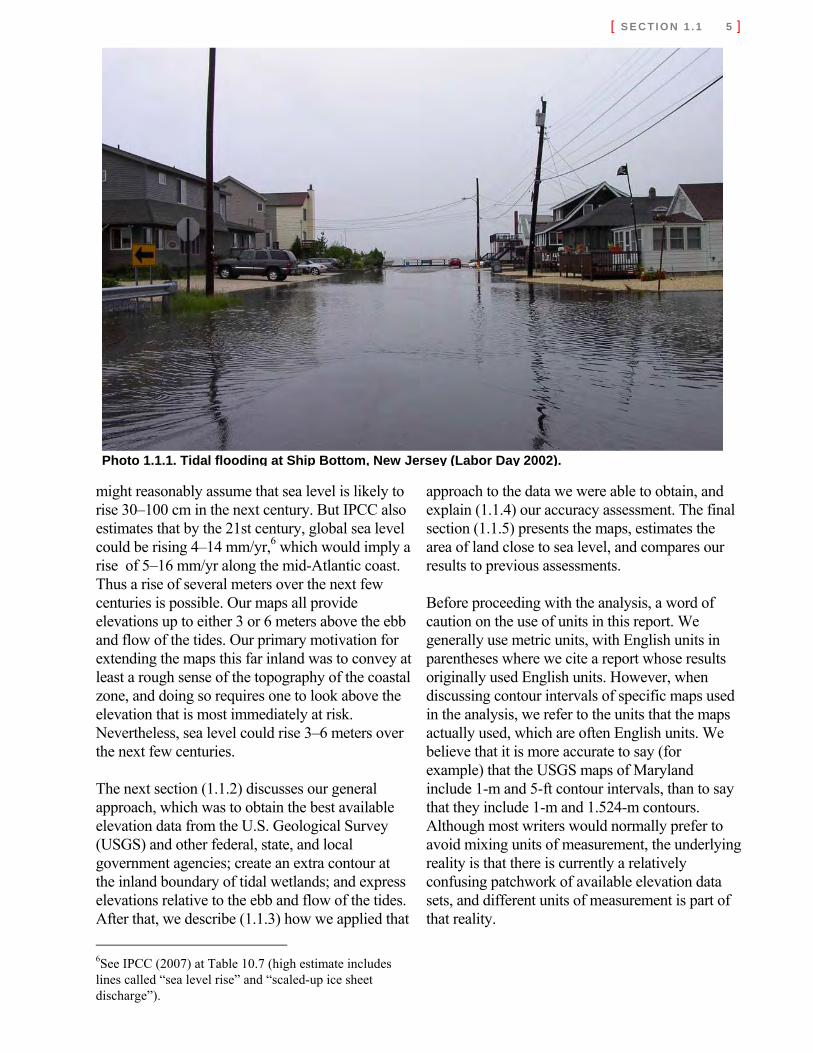
might reasonably assume that sea level is likely to rise 30–100 cm in the next century. But IPCC also estimates that by the 21st century, global sea level could be rising 4–14 mm/yr,6 which would imply a rise of 5–16 mm/yr along the mid-Atlantic coast. Thus a rise of several meters over the next few centuries is possible. Our maps all provide elevations up to either 3 or 6 meters above the ebb and flow of the tides. Our primary motivation for extending the maps this far inland was to convey at least a rough sense of the topography of the coastal zone, and doing so requires one to look above the elevation that is most immediately at risk. Nevertheless, sea level could rise 3–6 meters over the next few centuries. The next section (1.1.2) discusses our general approach, which was to obtain the best available elevation data from the U.S. Geological Survey (USGS) and other federal, state, and local government agencies; create an extra contour at the inland boundary of tidal wetlands; and express elevations relative to the ebb and flow of the tides. After that, we describe (1.1.3) how we applied that

6See IPCC (2007) at Table 10.7 (high estimate includes lines called “sea level rise” and “scaled-up ice sheet discharge”).

approach to the data we were able to obtain, and explain (1.1.4) our accuracy assessment. The final section (1.1.5) presents the maps, estimates the area of land close to sea level, and compares our results to previous assessments. Before proceeding with the analysis, a word of caution on the use of units in this report. We generally use metric units, with English units in parentheses where we cite a report whose results originally used English units. However, when discussing contour intervals of specific maps used in the analysis, we refer to the units that the maps actually used, which are often English units. We believe that it is more accurate to say (for example) that the USGS maps of Maryland include 1-m and 5-ft contour intervals, than to say that they include 1-m and 1.524-m contours. Although most writers would normally prefer to avoid mixing units of measurement, the underlying reality is that there is currently a relatively confusing patchwork of available elevation data sets, and different units of measurement is part of that reality.

Photo 1.1.1. Tidal flooding at Ship Bottom, New Jersey (Labor Day 2002).

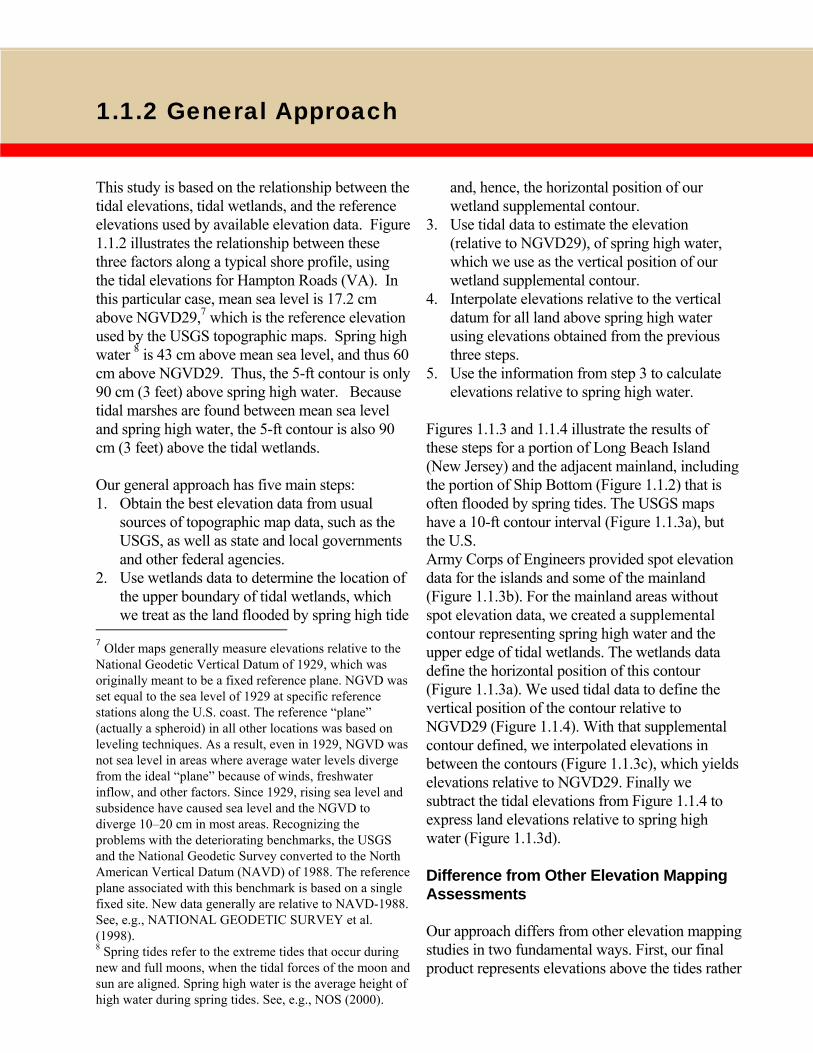
This study is based on the relationship between the tidal elevations, tidal wetlands, and the reference elevations used by available elevation data. Figure 1.1.2 illustrates the relationship between these three factors along a typical shore profile, using the tidal elevations for Hampton Roads (VA). In this particular case, mean sea level is 17.2 cm above NGVD29,7 which is the reference elevation used by the USGS topographic maps. Spring high water 8 is 43 cm above mean sea level, and thus 60 cm above NGVD29. Thus, the 5-ft contour is only 90 cm (3 feet) above spring high water. Because tidal marshes are found between mean sea level and spring high water, the 5-ft contour is also 90 cm (3 feet) above the tidal wetlands. Our general approach has five main steps: 1. Obtain the best elevation data from usual

sources of topographic map data, such as the USGS, as well as state and local governments and other federal agencies.

2. Use wetlands data to determine the location of the upper boundary of tidal wetlands, which we treat as the land flooded by spring high tide

7 Older maps generally measure elevations relative to the National Geodetic Vertical Datum of 1929, which was originally meant to be a fixed reference plane. NGVD was set equal to the sea level of 1929 at specific reference stations along the U.S. coast. The reference “plane” (actually a spheroid) in all other locations was based on leveling techniques. As a result, even in 1929, NGVD was not sea level in areas where average water levels diverge from the ideal “plane” because of winds, freshwater inflow, and other factors. Since 1929, rising sea level and subsidence have caused sea level and the NGVD to diverge 10–20 cm in most areas. Recognizing the problems with the deteriorating benchmarks, the USGS and the National Geodetic Survey converted to the North American Vertical Datum (NAVD) of 1988. The reference plane associated with this benchmark is based on a single fixed site. New data generally are relative to NAVD-1988. See, e.g., NATIONAL GEODETIC SURVEY et al. (1998). 8 Spring tides refer to the extreme tides that occur during new and full moons, when the tidal forces of the moon and sun are aligned. Spring high water is the average height of high water during spring tides. See, e.g., NOS (2000).

and, hence, the horizontal position of our wetland supplemental contour.

3. Use tidal data to estimate the elevation (relative to NGVD29), of spring high water, which we use as the vertical position of our wetland supplemental contour.

4. Interpolate elevations relative to the vertical datum for all land above spring high water using elevations obtained from the previous three steps.

5. Use the information from step 3 to calculate elevations relative to spring high water.

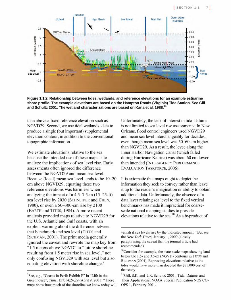
Figures 1.1.3 and 1.1.4 illustrate the results of these steps for a portion of Long Beach Island (New Jersey) and the adjacent mainland, including the portion of Ship Bottom (Figure 1.1.2) that is often flooded by spring tides. The USGS maps have a 10-ft contour interval (Figure 1.1.3a), but the U.S. Army Corps of Engineers provided spot elevation data for the islands and some of the mainland (Figure 1.1.3b). For the mainland areas without spot elevation data, we created a supplemental contour representing spring high water and the upper edge of tidal wetlands. The wetlands data define the horizontal position of this contour (Figure 1.1.3a). We used tidal data to define the vertical position of the contour relative to NGVD29 (Figure 1.1.4). With that supplemental contour defined, we interpolated elevations in between the contours (Figure 1.1.3c), which yields elevations relative to NGVD29. Finally we subtract the tidal elevations from Figure 1.1.4 to express land elevations relative to spring high water (Figure 1.1.3d). Difference from Other Elevation Mapping Assessments Our approach differs from other elevation mapping studies in two fundamental ways. First, our final product represents elevations above the tides rather

1.1.2 General Approach

[ S E C T I O N 1 . 1 7 ]

than above a fixed reference elevation such as NGVD29. Second, we use tidal wetlands data to produce a single (but important) supplemental elevation contour, in addition to the conventional topographic information. We estimate elevations relative to the sea because the intended use of these maps is to analyze the implications of sea level rise. Early assessments often ignored the difference between the NGVD29 and mean sea level. Because (local) mean sea level tends to be 10–20 cm above NGVD29, equating these two reference elevations was harmless when analyzing the impact of a 4.5–7.5-m (15–25-ft) sea level rise by 2030 (SCHNEIDER and CHEN, 1980), or even a 50–300-cm rise by 2100 (BARTH and TITUS, 1984). A more recent analysis provided maps relative to NGVD29 for the U.S. Atlantic and Gulf coasts, with an explicit warning about the difference between that benchmark and sea level (TITUS and RICHMAN, 2001). The print media generally ignored the caveat and rewrote the map key from “1.5 meters above NGVD” to “future shoreline resulting from 1.5 meter rise in sea level,” not only confusing NGVD29 with sea level but also equating elevation with shoreline change.9 9See, e.g., “Coasts in Peril: Exhibit E” in “Life in the Greenhouse”, Time, 157:14:24,29 (April 9, 2001) “These maps show how much of the shoreline we know today will

Unfortunately, the lack of interest in tidal datums is not limited to sea level rise assessments: In New Orleans, flood control engineers used NGVD29 and mean sea level interchangeably for decades, even though mean sea level was 50–60 cm higher than NGVD29. As a result, the levee along the Inner Harbor Navigation Canal (which failed during Hurricane Katrina) was about 60 cm lower than intended (INTERAGENCY PERFORMANCE EVALUATION TASKFORCE, 2006). It is axiomatic that maps ought to depict the information they seek to convey rather than leave it up to the reader’s imagination or ability to obtain additional data. Unfortunately, the absence of a data layer relating sea level to the fixed vertical benchmarks has made it impractical for coarse-scale national mapping studies to provide elevations relative to the sea.10 As a byproduct of

vanish if sea levels rise by the indicated amount.” But see the New York Times, January 1, 2000 (closely paraphrasing the caveat that the journal article had recommended). 10Consider for example, the state-scale maps showing land below the 1.5- and 3.5-m (NGVD) contours in TITUS and RICHMAN (2001). Expressing elevations relative to the tides would have more than doubled the $75,000 cost of that study. 11Gill, S.K. and J.R. Schultz. 2001. Tidal Datums and Their Applications, NOAA Special Publication NOS CO-OPS 1, February 2001.

Figure 1.1.2. Relationship between tides, wetlands, and reference elevations for an example estuarine shore profile. The example elevations are based on the Hampton Roads (Virginia) Tide Station. See Gill and Schultz 2001. The wetland characterizations are based on Kana et al. 1988.11

[ 8 M AP S O F L AN D S C L O S E T O S E A L E V E L AL O N G T H E U . S . M I D D L E AT L AN T I C C O AS T ]

Map A Map B

Map C Map D

Figure 1.1.3. Estimated elevations around Long Beach Island, New Jersey. The first three maps show elevations relative to NGVD29 according to (a) the USGS 1:24,000 scale map, (b) spot elevations provided by the Corps of Engineers where available and USGS data elsewhere, and (c) our interpolations using wetlands data as a supplemental contour. The final map (d) shows the same elevations as (c), relative to spring high water. The first map also shows the location of spring tide flooding depicted in Photo 1.1.1.

[ S E C T I O N 1 . 1 9 ]

this effort, we create such a layer that others may find useful even as LIDAR becomes available.12 In ordinary conversations, people refer to elevations “above sea level.” This report provides elevations relative to spring high water instead, for two reasons: First, one can map the existing high water mark more accurately than mean sea level. Wetland maps generally show the upper boundary of tidal wetlands, but maps illustrating the location of the shore at mean tide level are rarely available. Second, showing elevations relative to high water is more useful than mean sea level, because the character of land changes fundamentally once it is subject to the ebb and flow of the tides: Marsh grasses replace trees, lawns, or crops that cannot tolerate the saltwater

12NOAA is developing a software tool that converts data between fixed benchmarks and elevations relative to the tides, making this aspect of our analysis obsolete as well in a few years. See, e.g., PARKER et al. (2003) and MYERS (2005). Results are available for Pamlico Sound, which we used.

and frequent flooding13 (see generally TEAL and TEAL, 1969). Moreover, the land becomes subject to tidal wetlands regulations,14 and ownership shifts from the upland owner to the public in most states (SLADE et al. 1990). By contrast, elevation above mean sea level implies little about the impact of sea level rise. Because tide ranges vary, knowing that a parcel is 50 cm above mean sea level does not tell one whether it is even wet or dry land, let alone the rise in sea level necessary to convert the area to open water. Difference from Other Sea Level Rise Impact Mapping Studies This effort also differs from most sea level rise impact mapping studies because we report elevations rather than projected future shorelines. Maps of future shorelines are important, but elevations alone say something about vulnerability to sea level rise. Converting our results into maps of future shorelines would represent, in effect, a separate study—and the final results would be more speculative. Elevation is a necessary precursor for estimating shoreline change due to sea level rise. But projecting future shorelines requires more questionable assumptions than one must make when estimating elevations. The Bruun (1962) Rule produces an approximation of sandy beach erosion that is useful for some purposes, but many geologists decline to project erosion of beaches without applying a more site-specific model 13This generalization does not always apply in areas with low salinity. In nanotidal areas (i.e., areas where the astronomic tide range is only a few centimeters) the “tidal wetland” vegetation may be irregularly flooded because of winds rather than regularly flooded from astronomic tides. There may be a gradual transition between the irregularly flooded wetlands and adjacent nontidal wetlands, and even if the line is well-defined, the elevation is not a function of the tides. The Pamlico and Albemarle sounds are the most important example in our study area. Other exceptions include tidal freshwater forests and areas where extensive tidal freshwater wetlands are adjacent to nontidal wetlands with similar vegetation types. 14Clean Water Act § 404, 33 U.S.C. § 1344(a) (1994) and Rivers and Harbors Act of 1899, 33 U.S.C. §§ 403, 409 (1994).

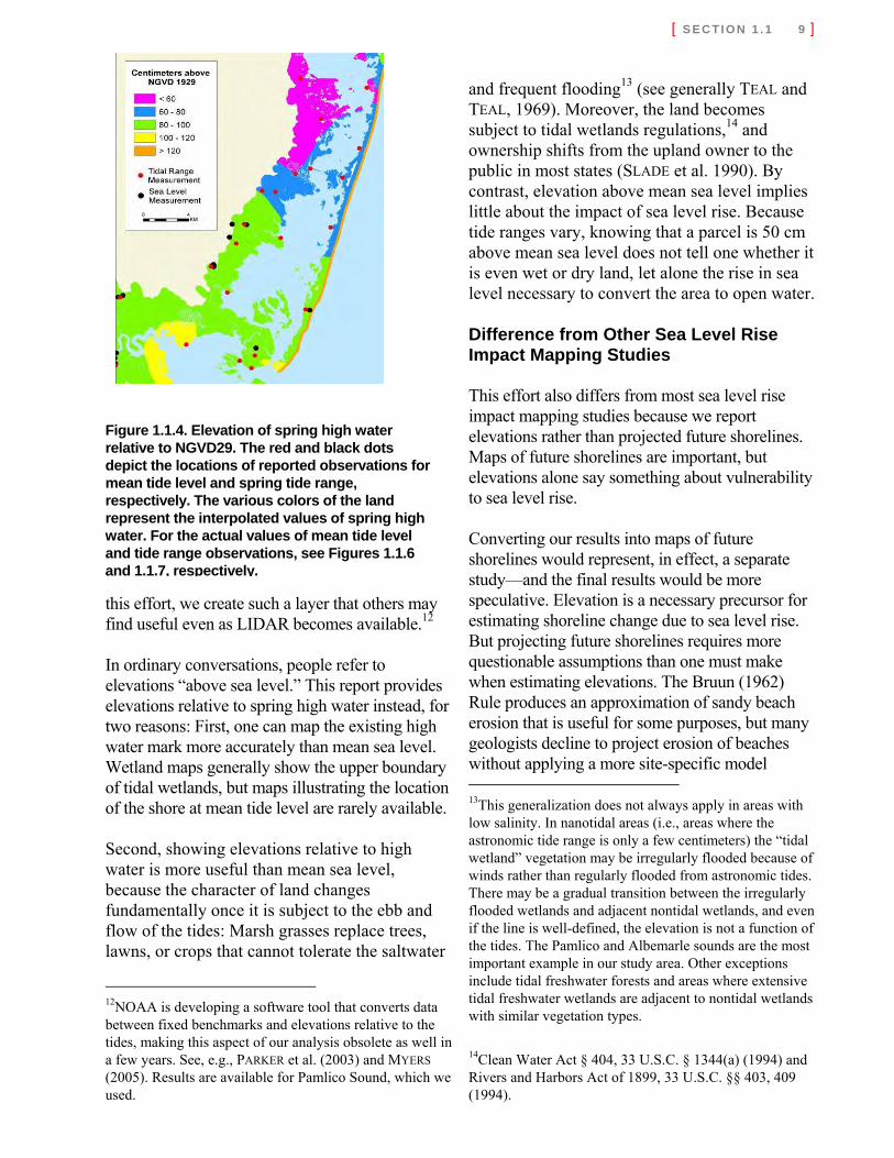
Figure 1.1.4. Elevation of spring high water relative to NGVD29. The red and black dots depict the locations of reported observations for mean tide level and spring tide range, respectively. The various colors of the land represent the interpolated values of spring high water. For the actual values of mean tide level and tide range observations, see Figures 1.1.6 and 1.1.7, respectively.

[ 10 M AP S O F L AN D S C L O S E T O S E A L E V E L AL O N G T H E U . S . M I D D L E AT L AN T I C C O AS T ]

requiring data collected over several years (e.g., DEAN and MAURMEYER, 1983; COWELL and THOM, 1994; COWELL et al., 1995; YOUNG and PILKEY, 1995). And sandy beaches are the best known shores! Wetland accretion is too poorly understood for coastal scientists to quantify how rapidly the sea could rise before it began to drown the wetlands (KANA et al., 1988; PARK et al., 1989; CAHOON et al., 1995).15 The ability to predict erosion of muddy shores is so poor that for many geologists, the term “coastal erosion” refers only to sandy beaches. Even in areas where we have a good model of shore erosion, projecting future shoreline can require a rather cumbersome set of analytical steps. Future sea level rise is uncertain; so one must evaluate the implications of several scenarios, taking care to ensure that one has encompassed the range of uncertainty. Different readers have different time horizons, so one typically must prepare maps for a few different projection years. Finally, actual shoreline migration will also depend on the type and extent of human activities to hold back the sea, so one must consider alternative shore-protection scenarios. Handling all these issues well on a regional scale requires too much effort to be undertaken as a final step of this study.

15Elsewhere in this report, however, a panel of wetland accretion specialists provide a consensus subjective assessment about whether mid-Atlantic wetlands could keep pace with three sea level rise scenarios. (See Reed et al., Section 2.1 of this report.)

Fortunately, coastal elevations do tell us something about the impacts and responses to sea level rise. Coastal wildlife managers who want to ensure that new wetlands are created as sea level rises must identify the dry land that might be tidally flooded in the future. The importance of reserving a given parcel depends on how much the sea has to rise before the tides inundate the land. The need to elevate streets and back yards depends on the land’s elevation. Moreover, an elevation map makes a suitable graphic for those attempting to convey the broad ramifications of sea level rise to the general public because it shows both existing wetlands and the dry land that will be inundated as the sea rises.

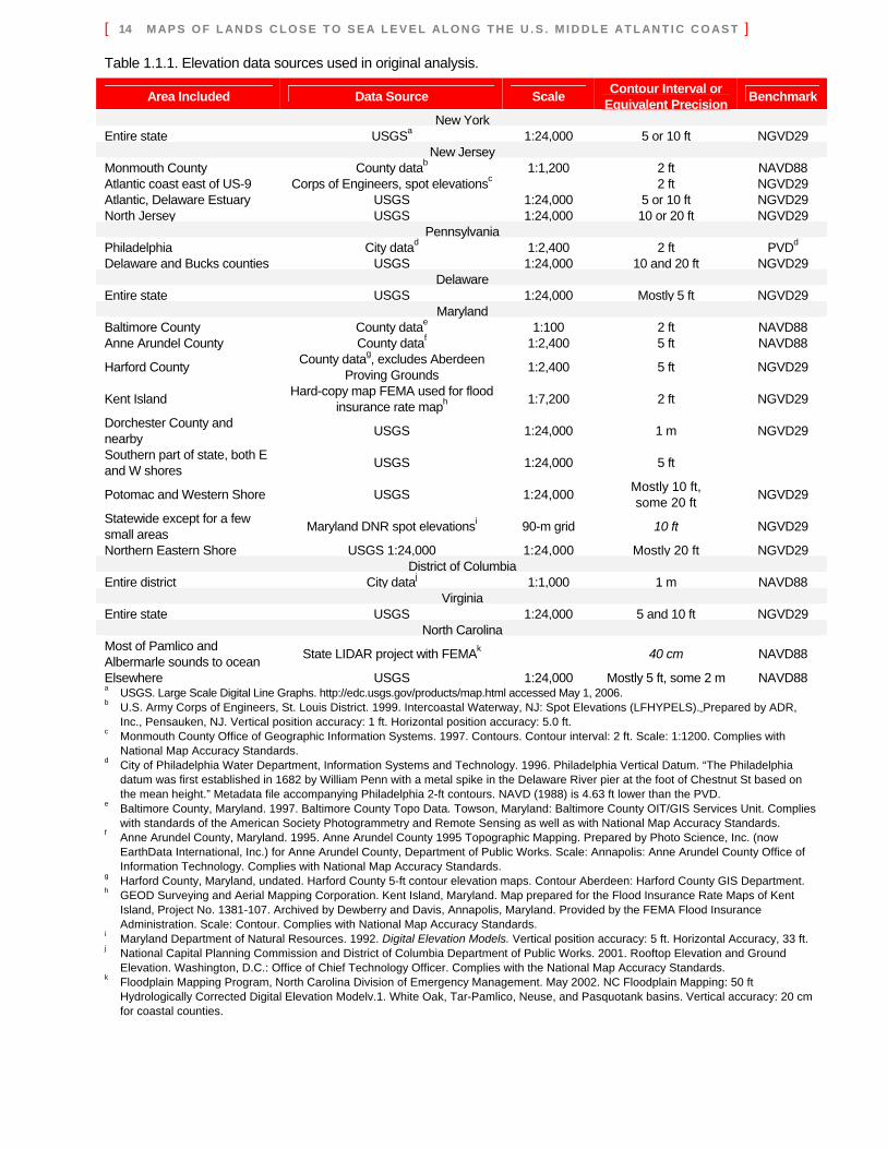
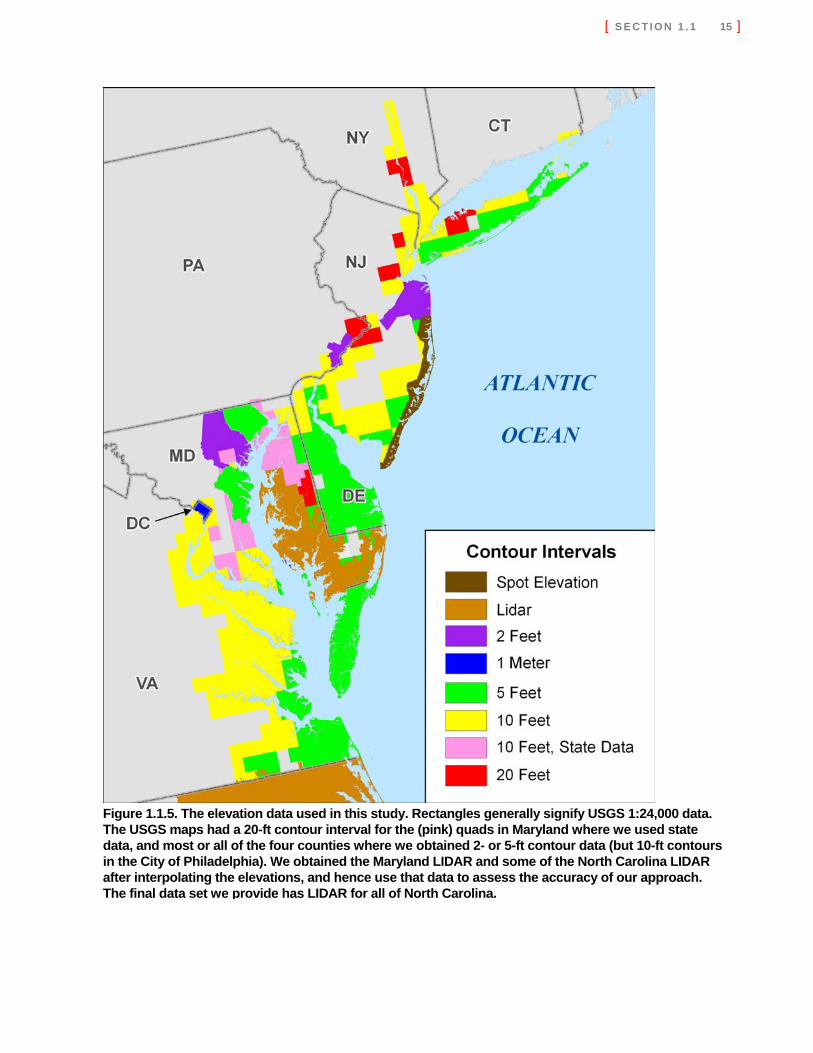
Step 1: Obtain Best Elevation Data Table 1.1.1 summarizes the elevation data we used. For a given state, the order in which the table lists the data represents the quality of the data and, hence, the order in which we selected data layers. For example, in Maryland, we used the 10-ft contour from the Department of Natural Resources spot elevation data set in areas where the USGS maps had a contour interval of 20 feet.16 If USGS 7.5-minute maps had a contour interval of 10 feet (or better), however, we preferred the USGS data. For four counties, we had county data with 2- or 5-ft contours, which was even better. Our approach was more systematic than one might initially assume, given the variation in data quality indicated by Table 1.1.1. Our goal was to estimate the land potentially inundated by a 1-m rise in sea level where possible and, where we could not, at least map the area vulnerable to a 2- or 3-m rise. Although we would have preferred to rely solely on a nationwide data set, the USGS 7.5-minute maps do not have a consistent contour interval—and for much of the coast their contour intervals are too great, especially in New Jersey and Maryland (see Figure 1.1.5). Therefore, we attempted to supplement the USGS data where feasible. Outside North Carolina, the USGS 5-ft contour is generally within 1 meter above the ebb and flow of the tides. Therefore, outside North Carolina, wherever the USGS maps had a contour interval of 5 feet or better, we did not actively seek better data.

16We obtained LIDAR for the lower Eastern Shore of Maryland after the analysis was complete. We use that data to assess the accuracy of our DEM in the section on Quality Control and Review. The primary data set we make available to the public will include these LIDAR data; we will also make the original data set available.

A 20-ft contour interval, by contrast, provides no information about lands vulnerable to sea level rise in any meaningful time horizon (although it does identify areas that are not vulnerable). Therefore, we made a relatively exhaustive effort to obtain alternative data in the portions of New Jersey and Maryland where the USGS maps had a 20-ft contour interval. Fortunately, Maryland had spot elevations on a 90-m grid with a vertical precision (90 percent interval) of 5 feet. Thus, according to national map accuracy standards (BUREAU OF THE BUDGET, 1947; Federal Geodetic Control Subcommittee, 1998), the Maryland data provide a 10-ft contour interval at a 1:180,000 scale. The horizontal scale is considerably poorer than the USGS 1:24,000 maps; but unlike a map with a 10-ft contour interval, the spot elevations provide estimates for points with intermediate elevations, allowing us to derive, for example, a 5-ft contour (albeit with twice the vertical error of national mapping standards). Unfortunately, New Jersey had no similar statewide data set. Many counties have elevation data for coastal floodplain management, pollution runoff modeling, and identification of areas where slopes make land undevelopable. Unlike the federal government, however, the counties usually charge for the data—sometimes tens of thousands of dollars per quad. In some cases, the bonds used to raise the money to collect the data contain restrictions against giving the data away.17 The restrictive county policies generally allow the GIS department to provide the data to a genuine partner doing work primarily to benefit the county. This study probably would not—by itself—qualify because we are analyzing the vulnerability of a multistate region to rising sea level and creating a product for researchers who will not, in general, collaborate with county staff to attain county objectives. Nevertheless, our collaboration with

17The planning director of Monmouth County, New Jersey, expressed this concern.

1.1.3 Application of Our Approach

[ 12 M AP S O F L AN D S C L O S E T O S E A L E V E L AL O N G T H E U . S . M I D D L E AT L AN T I C C O AS T ]

four counties led four county GIS departments to see this effort within the context of a joint federal–local partnership to understand the implications of rising sea level: • Monmouth County (New Jersey): The only

county along New Jersey’s Atlantic Coast where USGS maps have a 20-ft contour interval.

• Anne Arundel County (Maryland): This county includes both Annapolis and the largest low-lying area on Maryland’s Western Shore of Chesapeake Bay.

• Harford County (Maryland): This county includes the second largest area of very low-lying lands along the Western Shore.

• Baltimore County (Maryland). Unlike the other counties, Baltimore insisted that we provide elevation maps using their superior (2-ft contour) elevation data before they would even consider responses to sea level rise.

We also examined some maps that had been stored in the warehouse where FEMA keeps the documentation for the flood insurance rate maps. In general, whenever the USGS maps had contour intervals greater than 5 feet, FEMA obtained topographic maps. As a test, FEMA searched their archives for specific communities in Monmouth County, New Jersey, and found that for about half the townships and boroughs, the archives contained numerous maps with 2-ft contours at a scale better than 1:10,000. We were tempted to have those maps all digitized. FEMA, however, was reluctant to allow the entire collection to leave their premises—and we were not sure that the effort was worthwhile for areas with only partial coverage. We did persuade FEMA to lend us their map of Kent Island, Maryland, the eastern landing of the Chesapeake Bay Bridge, where our own

eyes told us that the land is very low but the USGS maps have a 20-ft contour interval. The supplemental data sources left us with only 24 quads where we have nothing better than a 20-ft contour interval.18 All of those quads are along tidal rivers well inland or upstream from a major estuary, except for six quads along the north shore of Long Island, which is dominated by substantial bluffs, and three quads in northern New Jersey (see Figure 1.1.5). Maps with 10-ft contour intervals give some insight on vulnerability to sea level rise, but not enough to justify their use if one can find a practical alternative. Unfortunately for us, most USGS maps have 10-ft contours in coastal New Jersey, New York, Pennsylvania, Virginia, the District of Columbia, and Virginia west of Chesapeake Bay. For most low land along the Atlantic Ocean and back barrier bays in New Jersey (except for Monmouth County, where we had 2-ft contours), the Corps of Engineers provided spot elevations with sufficient precision and density to identify 4-ft contour intervals at a 1:100,000 scale. The District of Columbia provided 1-m contour data. The City of Philadelphia provided 2-ft contours. Most of Pennsylvania’s remaining low land is in Delaware County; because of the high tide range, the 10-ft contours in that region are only about 150 cm (5 feet) above spring high water. North Carolina is a special case. Currituck, Pamlico, and Albemarle sounds have almost no tides because the areas of these bodies of water are large compared to their inlets to the ocean. With the high water mark barely above sea level, the sea would have to rise more than 1 meter to inundate the 5-ft contour during a high tide, unlike areas with larger tidal ranges. In the wake of Hurricane Floyd, however, the state collaborated with FEMA to substantially improve the already-good elevation data with LIDAR. Early on in the study,

18Those 24 quads also included all or part of the upper tidal portions of the Delaware River (Bucks County, Pennsylvania, and Burlington County, New Jersey), Choptank River (Caroline County, Maryland) Wicomico River (Worcester County, Maryland), and several small rivers or creeks in New Jersey.

[ S E C T I O N 1 . 1 13 ]

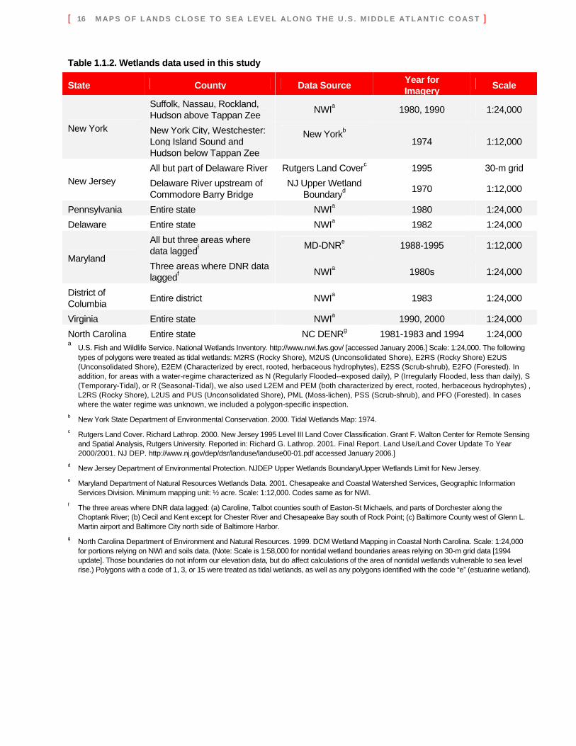
we obtained LIDAR for most of the low-lying counties in the state19; and by the end of the study we had data for the entire state. As we discuss below, however, the absence of tides and tide data for this area diminishes the usefulness of our analysis for evaluating the possible impacts of sea level rise in North Carolina. Step 2: Use Wetlands Data to Obtain the Location of the Upper Boundary of Tidal Wetlands We used tidal wetlands to define a supplemental topographic contour, approximately equal to spring high water. The precise elevation of that contour varies, but it is almost always between zero and the lowest contour above zero. This supplemental contour is useful and important for two reasons: First, for many purposes we are interested in knowing elevations above the tides; so a contour that defines the upper boundary of the tides is essential. Second, where elevation information is poor, a supplemental contour is likely to be more accurate than elevations estimated by interpolating with a model. Table 1.1.2 lists our wetlands data sources. Just as the USGS provides 7.5-minute quadrangles at a 1:24,000 scale for topography, so too the US Fish and Wildlife Service’s National Wetlands Inventory (NWI) provides 1:24,000 maps with broad wetland categories. Several states, however, have developed their own wetlands maps; representatives from New Jersey, Maryland, and North Carolina asked us to use their data instead of the NWI maps.20 The key limitation of the NWI data is its age: the aerial photographs for New Jersey were from the 1970s, and the Maryland and North Carolina 19As we discuss, we obtained LIDAR for the rest of the state after we developed our elevation data. As with the Eastern Shore of Maryland, we use these data to assess the accuracy of our procedure and will make the better LIDAR data available to the public. 20New York also provided wetland data for a portion of its coastal zone. Delaware also has its own wetland data, but state officials did not specifically ask us to use their data, and given the cost of interpreting each new data set, we did not.

photographs were from the 1980s.21 Since then wetland shores have eroded, low dry land areas have converted to wetlands, human activities have converted wetlands to dry land,22 and some previously drained areas have converted back to wetlands.23 A second limitation of NWI is scale. Small fringing wetlands along tidal creeks sometimes do not show up in the NWI data set, even though they are large enough to be seen on a 1:24,000 scale map. Given these limitations, and the availability of data that state agencies trust more for their uses, we took the three states' advice and used their data. We use wetlands only to define the inland limit of tidal wetlands. Kana et al. (1988) originally proposed the approach that we apply here. While surveying marsh transects around Charleston (South Carolina) and Long Beach Island (New Jersey), they recalled that low marsh is generally flooded twice daily and high marsh is flooded at spring tides but not every day. With an estimate of mean high water and spring high water, they reasoned, the wetland zonation can give supplemental elevation contours at both mean high water24 and spring high water. PARK et al. (1989) first applied that approach. Although their LANDSAT imagery did not distinguish between low and high marsh vegetation, PARK et al. attempted to do so by obtaining imagery at high tide during "half moons" (i.e., at mean high water) and delineating the flooded areas. The NWI and state wetlands data we used, however, made no such distinctions.

21See NWI Status Photo Page, accessed April 1, 2005, at http://www.nwi.fws.gov/statusphotoage.htm. 22Tidal wetlands are rarely converted to dry land for development, but occasionally some loss will be permitted for water-dependent uses such as marinas and ports. See generally U.S. EPA and U.S. Army Corps of Engineers (1990) (explaining the federal policy on wetland mitigation under section 404(b)(1) of the Clean Water Act). 23Along Delaware Bay, for example, diked wetlands had been converted to agriculture for more than a century. As part of an environmental mitigation program for a PSE&G nuclear power plant, most of the coastal zones of Cumberland County, New Jersey, and areas across the Bay in Delaware are being returned to nature. 24Mean high water is the average water level at high tide.

[ 14 M AP S O F L AN D S C L O S E T O S E A L E V E L AL O N G T H E U . S . M I D D L E AT L AN T I C C O AS T ]

Table 1.1.1. Elevation data sources used in original analysis.

Area Included Data Source Scale Contour Interval or Equivalent Precision Benchmark

New York Entire state USGSa 1:24,000 5 or 10 ft NGVD29

New Jersey Monmouth County County datab 1:1,200 2 ft NAVD88 Atlantic coast east of US-9 Corps of Engineers, spot elevationsc 2 ft NGVD29 Atlantic, Delaware Estuary USGS 1:24,000 5 or 10 ft NGVD29 North Jersey USGS 1:24,000 10 or 20 ft NGVD29

Pennsylvania Philadelphia City datad 1:2,400 2 ft PVDd Delaware and Bucks counties USGS 1:24,000 10 and 20 ft NGVD29

Delaware Entire state USGS 1:24,000 Mostly 5 ft NGVD29

Maryland Baltimore County County datae 1:100 2 ft NAVD88 Anne Arundel County County dataf 1:2,400 5 ft NAVD88

Harford County County datag, excludes Aberdeen Proving Grounds 1:2,400 5 ft NGVD29

Kent Island Hard-copy map FEMA used for flood insurance rate maph 1:7,200 2 ft NGVD29

Dorchester County and nearby USGS 1:24,000 1 m NGVD29

Southern part of state, both E and W shores USGS 1:24,000 5 ft

Potomac and Western Shore USGS 1:24,000 Mostly 10 ft, some 20 ft NGVD29

Statewide except for a few small areas Maryland DNR spot elevationsi 90-m grid 10 ft NGVD29

Northern Eastern Shore USGS 1:24,000 1:24,000 Mostly 20 ft NGVD29 District of Columbia

Entire district City dataj 1:1,000 1 m NAVD88 Virginia

Entire state USGS 1:24,000 5 and 10 ft NGVD29 North Carolina

Most of Pamlico and Albermarle sounds to ocean State LIDAR project with FEMAk 40 cm NAVD88

Elsewhere USGS 1:24,000 Mostly 5 ft, some 2 m NAVD88 a USGS. Large Scale Digital Line Graphs. http://edc.usgs.gov/products/map.html accessed May 1, 2006. b U.S. Army Corps of Engineers, St. Louis District. 1999. Intercoastal Waterway, NJ: Spot Elevations (LFHYPELS). Prepared by ADR,

Inc., Pensauken, NJ. Vertical position accuracy: 1 ft. Horizontal position accuracy: 5.0 ft. c Monmouth County Office of Geographic Information Systems. 1997. Contours. Contour interval: 2 ft. Scale: 1:1200. Complies with

National Map Accuracy Standards. d City of Philadelphia Water Department, Information Systems and Technology. 1996. Philadelphia Vertical Datum. “The Philadelphia

datum was first established in 1682 by William Penn with a metal spike in the Delaware River pier at the foot of Chestnut St based on the mean height.” Metadata file accompanying Philadelphia 2-ft contours. NAVD (1988) is 4.63 ft lower than the PVD.

e Baltimore County, Maryland. 1997. Baltimore County Topo Data. Towson, Maryland: Baltimore County OIT/GIS Services Unit. Complies with standards of the American Society Photogrammetry and Remote Sensing as well as with National Map Accuracy Standards.

f Anne Arundel County, Maryland. 1995. Anne Arundel County 1995 Topographic Mapping. Prepared by Photo Science, Inc. (now EarthData International, Inc.) for Anne Arundel County, Department of Public Works. Scale: Annapolis: Anne Arundel County Office of Information Technology. Complies with National Map Accuracy Standards.

g Harford County, Maryland, undated. Harford County 5-ft contour elevation maps. Contour Aberdeen: Harford County GIS Department. h GEOD Surveying and Aerial Mapping Corporation. Kent Island, Maryland. Map prepared for the Flood Insurance Rate Maps of Kent

Island, Project No. 1381-107. Archived by Dewberry and Davis, Annapolis, Maryland. Provided by the FEMA Flood Insurance Administration. Scale: Contour. Complies with National Map Accuracy Standards.

i Maryland Department of Natural Resources. 1992. Digital Elevation Models. Vertical position accuracy: 5 ft. Horizontal Accuracy, 33 ft. j National Capital Planning Commission and District of Columbia Department of Public Works. 2001. Rooftop Elevation and Ground

Elevation. Washington, D.C.: Office of Chief Technology Officer. Complies with the National Map Accuracy Standards. k Floodplain Mapping Program, North Carolina Division of Emergency Management. May 2002. NC Floodplain Mapping: 50 ft

Hydrologically Corrected Digital Elevation Modelv.1. White Oak, Tar-Pamlico, Neuse, and Pasquotank basins. Vertical accuracy: 20 cm for coastal counties.

[ S E C T I O N 1 . 1 15 ]

Figure 1.1.5. The elevation data used in this study. Rectangles generally signify USGS 1:24,000 data. The USGS maps had a 20-ft contour interval for the (pink) quads in Maryland where we used state data, and most or all of the four counties where we obtained 2- or 5-ft contour data (but 10-ft contours in the City of Philadelphia). We obtained the Maryland LIDAR and some of the North Carolina LIDAR after interpolating the elevations, and hence use that data to assess the accuracy of our approach. The final data set we provide has LIDAR for all of North Carolina.

[ 16 M AP S O F L AN D S C L O S E T O S E A L E V E L AL O N G T H E U . S . M I D D L E AT L AN T I C C O AS T ]

Table 1.1.2. Wetlands data used in this study

State County Data Source Year for Imagery Scale

Suffolk, Nassau, Rockland, Hudson above Tappan Zee NWIa 1980, 1990 1:24,000

New York New York City, Westchester: Long Island Sound and Hudson below Tappan Zee

New Yorkb

1974 1:12,000

All but part of Delaware River Rutgers Land Coverc 1995 30-m grid New Jersey Delaware River upstream of

Commodore Barry Bridge NJ Upper Wetland

Boundaryd 1970 1:12,000

Pennsylvania Entire state NWIa 1980 1:24,000 Delaware Entire state NWIa 1982 1:24,000

All but three areas where data laggedf MD-DNRe 1988-1995 1:12,000

Maryland Three areas where DNR data laggedf NWIa 1980s 1:24,000

District of Columbia Entire district NWIa 1983 1:24,000

Virginia Entire state NWIa 1990, 2000 1:24,000 North Carolina Entire state NC DENRg 1981-1983 and 1994 1:24,000 a U.S. Fish and Wildlife Service. National Wetlands Inventory. http://www.nwi.fws.gov/ [accessed January 2006.] Scale: 1:24,000. The following

types of polygons were treated as tidal wetlands: M2RS (Rocky Shore), M2US (Unconsolidated Shore), E2RS (Rocky Shore) E2US (Unconsolidated Shore), E2EM (Characterized by erect, rooted, herbaceous hydrophytes), E2SS (Scrub-shrub), E2FO (Forested). In addition, for areas with a water-regime characterized as N (Regularly Flooded--exposed daily), P (Irregularly Flooded, less than daily), S (Temporary-Tidal), or R (Seasonal-Tidal), we also used L2EM and PEM (both characterized by erect, rooted, herbaceous hydrophytes) , L2RS (Rocky Shore), L2US and PUS (Unconsolidated Shore), PML (Moss-lichen), PSS (Scrub-shrub), and PFO (Forested). In cases where the water regime was unknown, we included a polygon-specific inspection.

b New York State Department of Environmental Conservation. 2000. Tidal Wetlands Map: 1974. c Rutgers Land Cover. Richard Lathrop. 2000. New Jersey 1995 Level III Land Cover Classification. Grant F. Walton Center for Remote Sensing

and Spatial Analysis, Rutgers University. Reported in: Richard G. Lathrop. 2001. Final Report. Land Use/Land Cover Update To Year 2000/2001. NJ DEP. http://www.nj.gov/dep/dsr/landuse/landuse00-01.pdf accessed January 2006.]

d New Jersey Department of Environmental Protection. NJDEP Upper Wetlands Boundary/Upper Wetlands Limit for New Jersey. e Maryland Department of Natural Resources Wetlands Data. 2001. Chesapeake and Coastal Watershed Services, Geographic Information

Services Division. Minimum mapping unit: ½ acre. Scale: 1:12,000. Codes same as for NWI. f The three areas where DNR data lagged: (a) Caroline, Talbot counties south of Easton-St Michaels, and parts of Dorchester along the

Choptank River; (b) Cecil and Kent except for Chester River and Chesapeake Bay south of Rock Point; (c) Baltimore County west of Glenn L. Martin airport and Baltimore City north side of Baltimore Harbor.

g North Carolina Department of Environment and Natural Resources. 1999. DCM Wetland Mapping in Coastal North Carolina. Scale: 1:24,000 for portions relying on NWI and soils data. (Note: Scale is 1:58,000 for nontidal wetland boundaries areas relying on 30-m grid data [1994 update]. Those boundaries do not inform our elevation data, but do affect calculations of the area of nontidal wetlands vulnerable to sea level rise.) Polygons with a code of 1, 3, or 15 were treated as tidal wetlands, as well as any polygons identified with the code “e” (estuarine wetland).

[ S E C T I O N 1 . 1 17 ]

New Jersey and North Carolina were special cases. For most of New Jersey, we used the 30-m grid data developed by Richard Lathrop for the State of New Jersey. These data provide a more detailed vegetation classification system, and it would have been possible to differentiate low from high marsh.25 For much of North Carolina, by contrast, we lacked the wetlands data necessary to completely apply our approach. Pamlico and Albemarle sounds, as well as their tributaries, are nanotidal estuaries: their astronomic tide ranges are so small that for most practical purposes there are no tides. As a result, wetlands data sets misleadingly classify the wetlands along the shore as “nontidal wetlands.” Unlike true nontidal wetlands, these wetlands are at sea level and experience the full force of the tides in the bodies of water to which they are attached. Thus, unlike nontidal wetlands, which would eventually be inundated by a rising sea level, the nanotidal wetlands are already inundated. But the wetlands data do not distinguish the nanotidal wetlands from the nontidal wetlands (other than areas where salinities are high enough in the estuary to support brackish marsh). Thus, the wetlands data do not provide the location for the supplemental contour we would have hoped to create. North Carolina’s LIDAR provided us with better elevation data than we would have been able to derive using the wetlands data; but the failure of the data to distinguish nontidal wetlands from nanotidal wetlands changes the meaning of any estimates of the area of tidal wetlands in North Carolina. Step 3: Use Information on Tide Ranges and Benchmark Elevations to Estimate the Absolute Elevation of the Upper Boundary of Tidal Wetlands

Creating a supplemental contour using wetlands data requires us to have an estimate of the elevation of the upper tidal wetland boundary. That elevation depends on the elevation of mean

25This study did not make such a differentiation. However, we provided the data for Ocean County for the study by Jones and Strange (Section 3.20 in Section 3 of this report), which did make such a distinction.

tide level26 (MTL) (relative to the benchmark) and the tidal range. Relate benchmark elevations to mean tide level. NOAA's Published Benchmark Sheets (NOS, 2005) and the corresponding National Geodetic Survey (NGS) Data Sheets27 provide estimates of the difference between mean tide level and the benchmark elevations at 125 locations throughout the study area. As Figure 1.1.6 shows, the majority of those locations are in or adjacent to New Jersey. Observations are especially sparse, by contrast, in the sounds of Long Island and North Carolina. Typically, mean tide level in the ocean is approx-imately 20–30 cm above NGVD29 in the mid-Atlantic, reflecting the rise in relative sea level since the benchmark was established. The average water level in a back bay, however, is often several centimeters higher than the mean tide level on the ocean side of the barrier island:28 The cross sections of inlets and channels are greater at high tide than low tide. As a result, a flood tide brings more water into the bay when the inlet is 1 meter above the bay than the ebb tide carries away when the inlet is 1 meter lower. Therefore, ignoring rainfall, the flows during the ebb and flood tides are in balance only if the average bay level is somewhat higher than the ocean. Rainfall and runoff are additional sources of water in estuaries, further increasing water levels relative to the nearby ocean. During wet periods, water levels in back bays behind barrier islands may be 10–30 cm higher than normal. This effect may be greatest in freshwater tidal rivers, given their distance from the ocean and prevailing seaward flow of water. Hence, as Figure 1.1.6 shows, mean tide level is higher at Philadelphia and Washington, D.C., than along the shores of 26Mean tide level is the average of mean high water and mean low water. It is generally very close to mean sea level (the average water level) but requires fewer data points to calculate. 27The Published Benchmark Sheets include links to the NGS information relating mean tide level to the vertical benchmark elevations. 28For example, the stations inside Little Egg Harbor Bay near Long Beach Island (New Jersey) show MTL to be about 1.25 feet above NGVD29.

[ 18 M AP S O F L AN D S C L O S E T O S E A L E V E L AL O N G T H E U . S . M I D D L E AT L AN T I C C O AS T ]

Delaware and Chesapeake bays, respectively. Along major bodies of water, the coverage is sufficient to estimate the elevation of mean tide level through interpolation.29 For back bays lacking such data, we assumed that the elevation of mean tide level was similar to that of a nearby bay where data are available. The complete lack of data for Albemarle and Pamlico sounds was the most problematic. Fortunately, we had the best land elevation data—LIDAR—for that area; thus our need for a supplemental contour based on wetlands and tidal data was least. NOAA has developed a hydraulic model to estimate water levels in Pamlico Sound, but not Albemarle Sound; we used the NOAA results wherever they were available (PARKER et al., 2003; MYERS, 2005). Use tidal range data to estimate the elevation of spring high water. Estimates of tide ranges are more prevalent than the absolute elevation of mean sea level. NOAA’s tide tables30 provide estimates31 of the mean and spring-tide range at 768 discrete locations in the study area (see Figure 1.1.7).32 As with the elevation of mean tide level, coverage is poor in Albemarle and Pamlico sounds, where astronomic tides are small compared to wind-generated tides; and again we used NOAA’s model for Pamlico Sound. The NOAA estimates consider only astronomic tides, whereas tidal wetlands are also found in areas that are flooded irregularly by the winds. The distinction is minor in areas with a large tidal range, but where astronomic tide ranges are small, 29We interpolated elevations using the TopoGrid function in ESRI’s ArcInfo Grid module (ESRI, 1998). See the section on Step 3 for additional details on interpolation algorithms. The algorithm allowed us to treat intervening land as a “barrier” in the interpolation. In a back bay, for example, we use measurements from the bay—but not nearby ocean locations, because the impoundment effect of an inlet can elevate mean tide level within the bay. 30See, e.g., NOS (2004). The hard-copy report “Tide Tables” is now provided online. In 2004 it was still called “Tide Tables” but more recent versions of the web site have dropped the traditional title. 31The estimates in the NOAA tide tables are long-term averages. 32Each USGS 1:24,000 scale map includes an estimate of the mean tide range, which PARK et al. (1989) used in their assessment.

the wind-generated tides tend to enable wetland vegetation to form tens of centimeters above mean tide level, even if the spring tide range is negligible. As with mean tide level, we used the available data to estimate the spring tide range through interpolation. We then calculated the elevation of spring high water relative to NGVD29 for the tidal epoch 1983–200133 as one-half the spring tide range plus the elevation of mean tide level calculated in the previous subsection. Based on various wetland transect studies relating wetland elevations to the tides (e.g., KANA et al., 1988), we assume that this elevation also represents the elevation of the upper boundary of tidal wetlands. This assumption is only an approximation: wetlands may extend above spring high water, for example, in areas with small tide ranges where winds frequently cause areas above spring high water to flood. This discrepancy will not affect our estimate of the amount of dry land within (for example) 50 cm above spring high water; but it does lead us to overlook that some of the land (for example) 50–75 cm above spring high water would be flooded enough to support tidal wetlands if sea level rises 50 cm. This error is small compared to the accuracy of most USGS topographic maps—but it would be very significant in areas where LIDAR is available.34 33NOAA’s Published Benchmark Sheets adjust estimates of mean tide level so that they refer to the mean tide level averaged over a 18.6-yr lunar cycle. See, e.g., GILL and SCHULTZ (2001). 34Commenting on this report, Christopher Spaur of the Corps of Engineers provided the following: Regularly flooded tidal marshes have a predictable—and easily ascertainable—flooding regime controlled by astronomical tides, and along the Atlantic Coast possess broad areas dominated by tall-form Spartina alterniflora. Irregularly flooded marshes are found in areas where the pattern of flooding is at most partly related to astronomical tidal regime instead of wind and seasonal tides (e.g., wet and dry periods causing water levels to vary). These marshes lack the pronounced break between tall-form Spartina alterniflora and other marsh plants that occurs in regularly flooded marshes (Frey and Basan, 1985). Surfaces are subject to long periods of exposure and inundation (Stout, 1988). Because duration of inundation determines the lower limits of marshes, the longer duration of inundation causes the lower limit of marshes to be higher than in an area where tides dominate. The surface of irregularly

[ S E C T I O N 1 . 1 19 ]

How accurate is our surface estimating spring high water? The NOAA data on spring tide range and mean tide level are based on substantial data and thus are precise for our purposes. Interpolation model error, however, can be significant. In large estuaries with substantial data, the variations of spring tide range from location to location are on the order of 5 cm; hence our interpolation error is likely to be small. In back barrier bays, however, tide ranges can vary by tens of centimeters. In many cases, the tide range simply dampens away from the inlets, and interpolation between stations can largely account for this dampening. In some cases, however, there are tidal creeks with no tide stations. In these locations, our error in calculating spring tide range—and hence spring high water—is likely to be on the order of tens of centimeters. Adjusting tidal elevations to account for sea level rise. Only by sheer coincidence would the wetland maps be based on imagery taken during the midpoint of the 19.6-year tidal epoch that NOAA used to define local mean sea level. Given our assumptions, the wetlands maps provide the location for spring high water the year the photos were taken. In parts of New Jersey, sea level has risen 10 cm since the photos were taken (e.g., PERMANENT SERVICE FOR MEAN SEA LEVEL, 2003). Even though this discrepancy is less than 5 cm in most areas, we corrected for it because it is a systematic error that can be corrected, unlike the substantial random error resulting from large contour intervals of most elevation data. We used the regression coefficients published by the Permanent Service for Mean Sea Level35 for all locations with more than 40 years of data (see Figure 1.1.1). We then estimated the current rate of sea level rise at intermediate locations through interpolation. Multiplying that rate by the number flooded marsh occurs at about mean high water (Reimold, 1977). In the coastal bays, where tidal range is generally 30–50 cm, the elevation range across the marsh surface is much less and the marshes tend to lack much habitat below MHW or so. The short form of Spartina alterniflora is dominant on the seaward edge, and the tall form is either lacking or very local in occurrence along tidal creeks. 35The Service obtains the data for the United States from NOAA’s National Ocean Service.

of years between the map date and the NOAA base year provided us with site-specific adjustments to our surface estimating the elevation of spring high water. Step 4: Interpolate Elevations Relative to the Vertical Datum for All Land above the Tidal Wetlands Using Elevations Obtained from the Previous Three Steps From the aforementioned steps, we had the standard elevation contours, plus a supplemental contour along the upper boundary of tidal wetlands. We now examine how we used those contours to characterize elevations of locations between the contours. Doing so required us to decide on a rule for addressing data conflicts and pick an interpolation algorithm. The primary potential for data conflicts concerned discrepancies between topographic contours and the tidal wetland boundary.36 Along the Delaware River and parts of Delaware Bay, the upper edge of the tidal wetlands is about 4 to 5 feet (NGVD29), so we expected the wetland boundary to occasionally be landward of the 5-ft contour. In areas with 2-ft and 1-m contours, we expected to see a similar overlap even in areas with low tidal ranges. We limited ourselves to two possible solutions: Either the wetlands data or the contour always takes precedence over the other. We decided that the wetlands data should take precedence over the contour information, for three reasons. First, accepting both data sets at face value, the elevation and wetlands data typically had a scale of 1:24,000 and hence an allowable horizontal error of 12 m. But the topographic maps also have a vertical error of one-half contour interval. Therefore, by its very terms, the typical topographic map allows for the possibility that the 5-ft contour may be as low as 75 cm (2.5 ft) (NGVD29), which would be tidal wetlands in most areas. Second, the wetlands data are newer.37 36With the exception of Maryland, we used only one source of standard topographic data in a given location. For Maryland, where we used USGS and MD-DNR information, the USGS contours took precedence. 37USGS has made planimetric updates to most of the maps since 1970. However, the contour dates are generally from

[ 20 M AP S O F L AN D S C L O S E T O S E A L E V E L AL O N G T H E U . S . M I D D L E AT L AN T I C C O AS T ]

Because of shore erosion, wetlands may now exist in areas that had previously been above the 10- or 20-ft contour. Finally, this approach leaves us with a reasonable landscape. If we gave precedence to the 5-ft contour, we would be left with a bluff over the wetlands along the 5-ft contour; removal of the 5-ft contour, by contrast, means that we interpolate between the wetlands and the 10-ft contour. In selecting an interpolation algorithm, we had to consider our three objectives: • Estimate the amount of land that could be

inundated by rising sea level to the level of precision allowable by existing data.

• Produce maps depicting the elevations of land close to sea level.

• Provide an elevation data set for other researchers.

Estimate the amount of land that could be inundated. The contours provide polygons of various elevation classifications. In a location with a 5-ft contour interval, for example, we have polygons that represent the land between spring high water and the 5-ft (152-cm) (NGVD29) contour, as well as 152 to 304 cm, etc. If spring high water happens to be 60 cm above NGVD29 in a given area, then we have polygons that tell us how much land is 0 to 92 cm above spring high water, as well as 92 to 244 cm, etc. However, contour intervals and the elevation of the tides vary, so the polygons in different locations represent different elevation ranges relative to the tides. This situation prevents us from simply adding the calculated area across all localities.38 Estimating the amount of land at particular elevations requires an assumption about how elevations are distributed in the land between the contours. We considered two approaches for estimating elevations between contours: using linear

the 1945–1970 period. See, e.g., the order forms provided by the New York State Center for Geographic Information (showing the planimetric and contour dates for every USGS 7.5-minute quad). Accessed on August 12, 2006, at http://www.nysgis.state.ny.us/mapssales/orderfrm/brantlk.htm. 38In areas where we have accurate spot elevations (e.g., LIDAR), we do not face this problem.

interpolation and using a digital elevation model (DEM) to fit an estimated land surface through the contour data we had. We tried the DEM approach first, because it was going to be necessary for creating the maps. We quickly concluded, however, that readily available algorithms would unreasonably skew our results. When the shore and the contours are all fairly straight or well-behaved, results seem reasonable; but when the contours have sharp turns, the algorithms assume that a disproportionate amount of land has an elevation close to that of the contour. In effect, the algorithms tend to create plateaus on either side of the contours.39 Therefore, our estimates are based on linear interpolations; i.e., we assume that elevation is uniformly distributed between contours. To keep the calculations manageable, we interpolated elevations at the quad level.40 Produce maps and elevation datasets. We interpolated between the contours and spot elevations using the TopoGrid algorithm provided by ESRI (1998) software. This procedure was developed based on Hutchinson’s (1988, 1989) approach to estimating DEMs. The fundamental insight embodied in that algorithm is that ground surfaces have many local peaks, but few local minimums, because water generally flows toward the sea rather than being impounded. For our purposes, that aspect was not important because we are not concerned about slopes; instead we are concerned with improving the accuracy of 39In Figure 1.1.8, TopoGrid correctly creates a stream valley in an area with a fairly simple topography. But when we applied that algorithm over our entire study area, we found numerous plateaus along the contours. Someone more skilled with the algorithm may have been able to set parameters to better replicate normal topography; but this algorithm was designed for correct drainage, not for correctly duplicating the distribution of elevations. 40For each quad, we estimated the average elevation of spring high water (SHW). We then calculated the amount of land between SHW and the 5-ft contour, and allocated it proportionally between 0 and 5-SHW. We then calculated the land between 5 and 10 feet and allocated it between 5-SHW and 10-SHW. We stored the results in bins of 0.1 feet. We followed this approach twice for each quad, so that we could distinguish nontidal wetlands from dry land (using nontidal wetlands polygons from the data sources displayed in Table 1.1.2).

[ S E C T I O N 1 . 1 21 ]

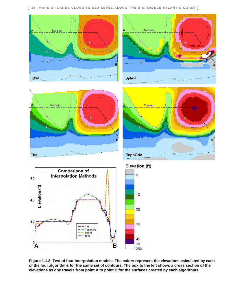
elevations at particular locations and correctly describing the overall distribution of elevations. Nevertheless, the algorithm’s use of stream data to characterize slopes should tend to ensure that stream valleys are captured below the lowest topographic contour, even in areas where the stream is above the tides (and hence would not provide a contour).41 We used a cell size of 30 meters because when we began the study, a 10-m cell size slowed processing time too much. Before settling on TopoGrid, we tested three other readily available algorithms: inverse distance weighting42 (IDW), spline,43 and triangulated irregular networks (TIN),44 using the (5-ft interval) contours in the general vicinity of Ocean City, Maryland. All four algorithms created plateaus near contours with sharp curves, with approximately the same amount of land having an elevation within 15 cm (0.5 feet) above or below the contour as the amount of land with an elevation 15 to 75 cm above or below the nearest contour. Figure 1.1.8 compares the four algorithms. Each started with the same set of set of contours, with a circular hill to the right, a U-shaped bluff to the left, a stream valley in between, and a shore that is otherwise fairly straight. The various colors represent the elevations that the four algorithms estimated. Between the 20- and 40- ft contours, the yellow-brown and pink-red shades in the TopoGrid and TIN maps suggest that these algorithms create intermediate elevation contours that are evenly spaced between the input contours. IDW, by contrast, assigns virtually all of this land to elevations of 20, 30, or 40 feet, as if the land 41If there is a 10-ft contour on either side of a creek, without additional information, an interpolation algorithm is likely to assume that the land between the contours (the stream valley) is also at 10 feet. 42IDW interpolates by defining the elevation of a point X as the weighted average of points A within a given neighborhood, with the weights being the inverse of the distance between X and the various points X, possibly raised to a power. See, e.g., SHEPARD (1968), FISHER et al. (1987), and CHILDS (2004). 43See, e.g., CHILDS (2004). 44A TIN is a digital data structure that represents terrain with a series of triangles. We used the ESRI command “CreateTin”. See, e.g., PRICE (1999).

were a series of steps. Spline creates 50-ft and 200-ft hills between the 20- and 30-ft contours for no obvious reasons. This example generally confirmed the literature: IDW is more appropriate when one has many points that already outline the shape of the surface (e.g., CHILDS, 2004). Spline tends to produce spurious hills, especially with unevenly spaced input data (e.g., ROGERS and SATTERFIELD, 1980; OLSEN and BLISS, 1997). Given the relatively large study area, we needed an algorithm that required less supervision than spline. Our choice between TIN and TopoGrid was a close call. In areas where the contours are one or two cells apart, TIN faithfully interpolates between the contours, whereas TopoGrid seems prone to horizontal errors of one or two cells. TIN completely misses the stream valley, however, treating both the valley and the U-shaped hill as a single flat area. TopoGrid, by contrast, creates a stream valley with a reasonably constant slope between the 10- and 20-ft contours. Similarly, TIN assumes that all the land within the 40-ft contour is at precisely 40 feet, whereas TopoGrid creates a peak in the center just above 45 feet. We decided to use TopoGrid because we were more willing to tolerate its one- or two-cell errors than maps that missed hills and streams. Step 5: Use the Information from Step 3 to Calculate Elevations Relative to Spring High Water We conducted both sets of interpolation relative to the fixed benchmark elevation. We created maps and a data set of elevations relative to spring high water by subtracting our estimate of the elevation of spring high water from every data point. We derived our estimates of the area of land within a given elevation above spring high water by subtracting the average elevation of spring high water within a given USGS quad from the elevation of the contours between which we were interpolating. The effect of this conversion is that our maps show the land below a given contour (e.g., USGS 5-ft contour) to be lower in areas with large tide ranges than in areas with small tide ranges.

[ 22 M AP S O F L AN D S C L O S E T O S E A L E V E L AL O N G T H E U . S . M I D D L E AT L AN T I C C O AS T ]

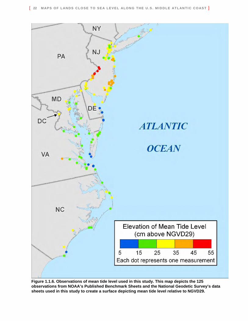
Figure 1.1.6. Observations of mean tide level used in this study. This map depicts the 125 observations from NOAA’s Published Benchmark Sheets and the National Geodetic Survey’s data sheets used in this study to create a surface depicting mean tide level relative to NGVD29.

[ S E C T I O N 1 . 1 23 ]

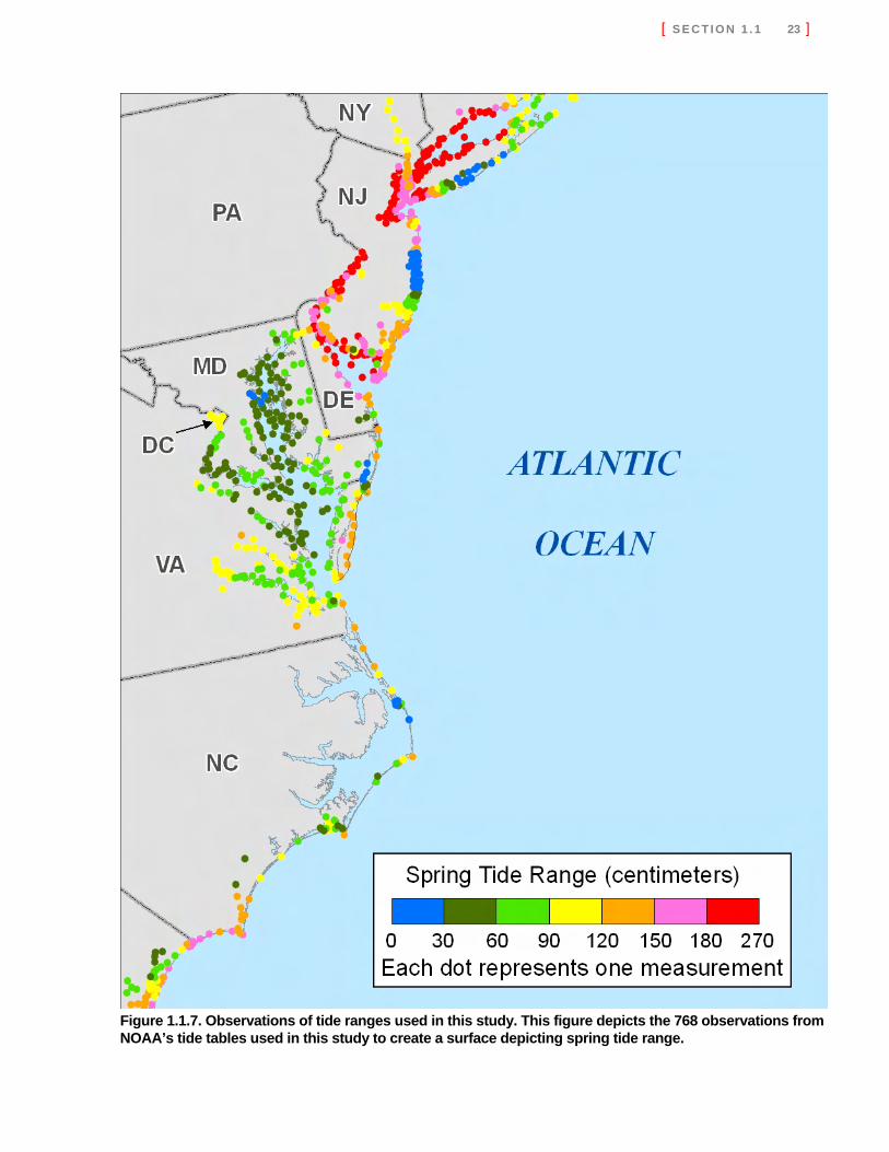
Figure 1.1.7. Observations of tide ranges used in this study. This figure depicts the 768 observations from NOAA’s tide tables used in this study to create a surface depicting spring tide range.

[ 24 M AP S O F L AN D S C L O S E T O S E A L E V E L AL O N G T H E U . S . M I D D L E AT L AN T I C C O AS T ]

Figure 1.1.8. Test of four interpolation models. The colors represent the elevations calculated by each of the four algorithms for the same set of contours. The box to the left shows a cross section of the elevations as one travels from point A to point B for the surfaces created by each algorithms.

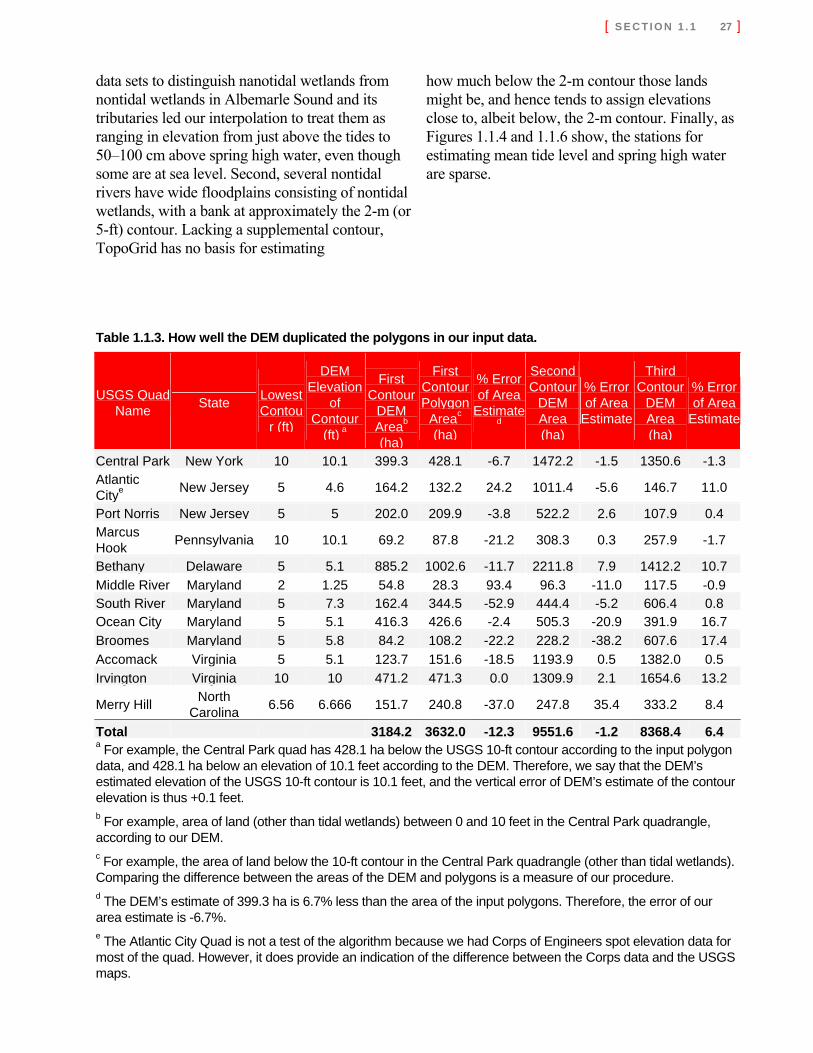
We corrected all the errors and questionable aspects that we noticed—but a test of what we did not notice was also necessary. We enlisted Russ Jones of Stratus Consulting to test the algorithm and validate the results against an independent data set. Let us briefly examine the results of the tests we asked him to perform. Testing the interpolation algorithm The intent of the algorithm is to interpolate between contours. Values that are outside the contours represent a failure, regardless of whether the problem is caused by TopoGrid or some other error. We asked Jones to pick 12 representative quads, including at least 1 quad for each state, encompassing the different contour intervals and data sources. After he picked the quads, we sent him the DEM (grid) results and the input data (see Table 1.1.1) representing polygons of land between the wetlands and the first contour (e.g., 5 ft), the first and second contour (e.g., 5–10 ft), etc. For each quad, we asked him to compare the areas of the source contour polygons with those of the interpolated DEM for the same elevation range and to produce a histogram of the DEM elevations by contour polygon. Table 1.1.3 shows the results of this comparison. Topogrid did not duplicate the area of dry land below the lowest contour as well as we had hoped, with percentage errors of 20 percent or more in 5 of the 12 quads. For the second and third contours, the percentage error was less than half as great, but hardly inspiring. The errors do not seem as large, however, when viewed as vertical error. The fourth column in Table 1.1.3 provides the “effective” elevation of the polygon contour as estimated by the DEM.45

45That is, the elevation below which the DEM estimates an area equal to the polygon area below the first contour.

For example, the polygon area below the 2-m contour of the Merry Hill quad is 241 ha. Although the DEM found only 152 ha below the 2-m (6.56-ft) contour, it also finds 241 below 6.67 ft.46 In 8 of the 12 quads, this effective elevation is less than 0.11 feet above the corresponding USGS contour. The area error is large and the vertical error is small, because the algorithm created a plateau along the contour; more land was slightly above the contour than slightly below it. Moreover, in most quads, most of the land below the first contour is tidal wetland. Hence, an error of 20 percent of the dry land is typically about 5 percent of the total land. Thus, if we included all low land in the denominator, our percentage error estimates for the lowest contour would have the same magnitude as for the other contours. This is particularly true for the Middle River quad in Baltimore County, Maryland, where the dry land below the 2-ft (NAVD88) contour is a very narrow strip adjacent to the tidal wetlands, whose inland boundary is often 1.5 feet above NAVD88. Thus, any such dry land in our data set may largely represent errors in the input data. We are unable to explain why our algorithm underestimated the low land below the first contour for the other 10 quads,47 but it may be an artifact related to the relative complexity of wetland shores. Comparing results with an independent dataset As this study proceeded, LIDAR data became available for the entire state of North Carolina as well as Maryland’s Eastern Shore south of Rock Hall (MD DNR, 2004). JONES (2007) converted 46For some of the quads, plateaus emerged at the contours in spite of our efforts to avoid them. 47We used Corps of Engineers spot elevation data for most of the Atlantic City quad, so the comparison with the USGS polygon area represents a comparison of Corps data to USGS maps more than a test of our algorithm.

1.1.4 Quality Control and Review: Error Estimation

[ 26 M AP S O F L AN D S C L O S E T O S E A L E V E L AL O N G T H E U . S . M I D D L E AT L AN T I C C O AS T ]

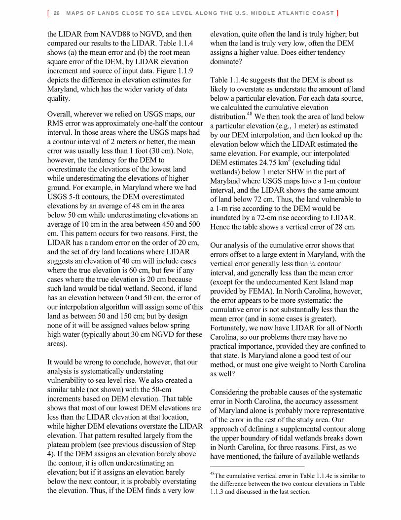
the LIDAR from NAVD88 to NGVD, and then compared our results to the LIDAR. Table 1.1.4 shows (a) the mean error and (b) the root mean square error of the DEM, by LIDAR elevation increment and source of input data. Figure 1.1.9 depicts the difference in elevation estimates for Maryland, which has the wider variety of data quality.

Overall, wherever we relied on USGS maps, our RMS error was approximately one-half the contour interval. In those areas where the USGS maps had a contour interval of 2 meters or better, the mean error was usually less than 1 foot (30 cm). Note, however, the tendency for the DEM to overestimate the elevations of the lowest land while underestimating the elevations of higher ground. For example, in Maryland where we had USGS 5-ft contours, the DEM overestimated elevations by an average of 48 cm in the area below 50 cm while underestimating elevations an average of 10 cm in the area between 450 and 500 cm. This pattern occurs for two reasons. First, the LIDAR has a random error on the order of 20 cm, and the set of dry land locations where LIDAR suggests an elevation of 40 cm will include cases where the true elevation is 60 cm, but few if any cases where the true elevation is 20 cm because such land would be tidal wetland. Second, if land has an elevation between 0 and 50 cm, the error of our interpolation algorithm will assign some of this land as between 50 and 150 cm; but by design none of it will be assigned values below spring high water (typically about 30 cm NGVD for these areas). It would be wrong to conclude, however, that our analysis is systematically understating vulnerability to sea level rise. We also created a similar table (not shown) with the 50-cm increments based on DEM elevation. That table shows that most of our lowest DEM elevations are less than the LIDAR elevation at that location, while higher DEM elevations overstate the LIDAR elevation. That pattern resulted largely from the plateau problem (see previous discussion of Step 4). If the DEM assigns an elevation barely above the contour, it is often underestimating an elevation; but if it assigns an elevation barely below the next contour, it is probably overstating the elevation. Thus, if the DEM finds a very low

elevation, quite often the land is truly higher; but when the land is truly very low, often the DEM assigns a higher value. Does either tendency dominate? Table 1.1.4c suggests that the DEM is about as likely to overstate as understate the amount of land below a particular elevation. For each data source, we calculated the cumulative elevation distribution.48 We then took the area of land below a particular elevation (e.g., 1 meter) as estimated by our DEM interpolation, and then looked up the elevation below which the LIDAR estimated the same elevation. For example, our interpolated DEM estimates 24.75 km2 (excluding tidal wetlands) below 1 meter SHW in the part of Maryland where USGS maps have a 1-m contour interval, and the LIDAR shows the same amount of land below 72 cm. Thus, the land vulnerable to a 1-m rise according to the DEM would be inundated by a 72-cm rise according to LIDAR. Hence the table shows a vertical error of 28 cm. Our analysis of the cumulative error shows that errors offset to a large extent in Maryland, with the vertical error generally less than ¼ contour interval, and generally less than the mean error (except for the undocumented Kent Island map provided by FEMA). In North Carolina, however, the error appears to be more systematic: the cumulative error is not substantially less than the mean error (and in some cases is greater). Fortunately, we now have LIDAR for all of North Carolina, so our problems there may have no practical importance, provided they are confined to that state. Is Maryland alone a good test of our method, or must one give weight to North Carolina as well? Considering the probable causes of the systematic error in North Carolina, the accuracy assessment of Maryland alone is probably more representative of the error in the rest of the study area. Our approach of defining a supplemental contour along the upper boundary of tidal wetlands breaks down in North Carolina, for three reasons. First, as we have mentioned, the failure of available wetlands 48The cumulative vertical error in Table 1.1.4c is similar to the difference between the two contour elevations in Table 1.1.3 and discussed in the last section.

[ S E C T I O N 1 . 1 27 ]

data sets to distinguish nanotidal wetlands from nontidal wetlands in Albemarle Sound and its tributaries led our interpolation to treat them as ranging in elevation from just above the tides to 50–100 cm above spring high water, even though some are at sea level. Second, several nontidal rivers have wide floodplains consisting of nontidal wetlands, with a bank at approximately the 2-m (or 5-ft) contour. Lacking a supplemental contour, TopoGrid has no basis for estimating

how much below the 2-m contour those lands might be, and hence tends to assign elevations close to, albeit below, the 2-m contour. Finally, as Figures 1.1.4 and 1.1.6 show, the stations for estimating mean tide level and spring high water are sparse.

Table 1.1.3. How well the DEM duplicated the polygons in our input data.

USGS Quad Name State

Lowest Contou

r (ft)

DEM Elevation

of Contour

(ft) a

First

Contour DEM Areab

(ha)

First Contour Polygon

Areac

(ha)

% Error of Area

Estimated

Second Contour

DEM Area (ha)

% Error of Area

Estimate

Third Contour

DEM Area (ha)

% Error of Area

Estimate

Central Park New York 10 10.1 399.3 428.1 -6.7 1472.2 -1.5 1350.6 -1.3 Atlantic Citye New Jersey 5 4.6 164.2 132.2 24.2 1011.4 -5.6 146.7 11.0

Port Norris New Jersey 5 5 202.0 209.9 -3.8 522.2 2.6 107.9 0.4 Marcus Hook Pennsylvania 10 10.1 69.2 87.8 -21.2 308.3 0.3 257.9 -1.7

Bethany Delaware 5 5.1 885.2 1002.6 -11.7 2211.8 7.9 1412.2 10.7 Middle River Maryland 2 1.25 54.8 28.3 93.4 96.3 -11.0 117.5 -0.9 South River Maryland 5 7.3 162.4 344.5 -52.9 444.4 -5.2 606.4 0.8 Ocean City Maryland 5 5.1 416.3 426.6 -2.4 505.3 -20.9 391.9 16.7 Broomes Maryland 5 5.8 84.2 108.2 -22.2 228.2 -38.2 607.6 17.4 Accomack Virginia 5 5.1 123.7 151.6 -18.5 1193.9 0.5 1382.0 0.5 Irvington Virginia 10 10 471.2 471.3 0.0 1309.9 2.1 1654.6 13.2

Merry Hill North Carolina 6.56 6.666 151.7 240.8 -37.0 247.8 35.4 333.2 8.4

Total 3184.2 3632.0 -12.3 9551.6 -1.2 8368.4 6.4 a For example, the Central Park quad has 428.1 ha below the USGS 10-ft contour according to the input polygon data, and 428.1 ha below an elevation of 10.1 feet according to the DEM. Therefore, we say that the DEM’s estimated elevation of the USGS 10-ft contour is 10.1 feet, and the vertical error of DEM’s estimate of the contour elevation is thus +0.1 feet. b For example, area of land (other than tidal wetlands) between 0 and 10 feet in the Central Park quadrangle, according to our DEM. c For example, the area of land below the 10-ft contour in the Central Park quadrangle (other than tidal wetlands). Comparing the difference between the areas of the DEM and polygons is a measure of our procedure. d The DEM’s estimate of 399.3 ha is 6.7% less than the area of the input polygons. Therefore, the error of our area estimate is -6.7%. e The Atlantic City Quad is not a test of the algorithm because we had Corps of Engineers spot elevation data for most of the quad. However, it does provide an indication of the difference between the Corps data and the USGS maps.

[ 28 M AP S O F L AN D S C L O S E T O S E A L E V E L AL O N G T H E U . S . M I D D L E AT L AN T I C C O AS T ]

Table 1.1.4. Accuracy of DEM Results: Comparison with LIDAR

Maryland Eastern Shore North Carolina Source: Kent Island 1-m 5-ft MD-DNR 20-ft 5 ft 2mContour (cm) 60 100 152 305 610 152 200

Elevationa A. Mean Error (Difference between DEM and LIDAR)b 50 60 26 48 102 17 58 56

100 12 18 9 74 -25 54 67150 0 56 27 71 -67 38 53200 4 23 54 72 -109 23 27250 -1 -7 43 59 -155 13 19300 -7 -9 21 37 -193 2 15350 -8 12 9 2 -240 -2 7400 -9 2 3 -35 -276 -4 1450 -13 -2 -3 -59 -304 -3 -5500 -42 -9 -10 -80 -341 2 -11

B. RMS Error (Root Mean Square Difference between LIDAR and DEM)c 50 102 38 107 160 18 113 116

100 74 59 70 151 28 92 92150 72 83 95 146 74 99 87200 80 41 100 135 124 100 84250 80 37 71 110 170 100 94300 76 52 56 91 218 91 96350 78 57 61 82 263 84 90400 94 49 63 84 308 77 81450 121 59 65 98 345 76 73500 135 71 66 119 387 86 73

C. Vertical Error (Difference in Cumulative Elevation Distribution)d 50 -48 3 -21 -36 -54 36 52

100 -65 28 -1 -19 -75 38 80150 -35 41 3 -18 -93 49 105200 -30 35 9 -7 -106 52 109250 -32 -3 23 -12 -110 46 130300 -30 1 10 -11 -113 52 115350 -29 -5 -2 -46 -111 73 67400 -21 -5 -6 -101 -108 94 68450 7 -14 -7 -104 -101 104 82500 16 -16 -8 * * 113 98

a In parts A and B, results are presented for 50-cm increments relative to NGVD29 as measured by LIDAR. For example, the second row in each case provides results averaged over all lands with elevations between 50 and 100 cm according to LIDAR. In part C, results are cumulative, and relative to spring high water as estimated by the DEM interpolations. For example, the second row is based on the area of land whose DEM interpolated elevation is less than 100 cm above SHW.

b The mean of LIDAR-DEM. For example, in parts of Maryland where USGS maps had a 5-ft contour and LIDAR showed elevations between 100 and 150 cm, the DEM estimate was 27 cm higher than the LIDAR value, on average. If LIDAR represents the true elevation, the mean difference represents mean error.

c Root mean square difference is calculated by taking the difference between the LIDAR and DEM elevations at each point, squaring that value, adding all the squares and dividing by the number of data points, then taking the square root. If the mean difference is zero, it is the same as the standard deviation. If LIDAR represents the true elevation, this value is the root mean square error.

d A measure of the sensitivity to sea level rise of an estimate of the amount of land vulnerable to inundation. For example, in parts of Maryland where USGS maps have a 1-m contour interval (excluding tidal wetlands), our interpolated DEM estimates 24.75 km2 below 1 meter, while the LIDAR shows the same amount of land below 72 cm. Assuming LIDAR to be accurate, the land vulnerable to a 1-m rise according to the DEM would actually be inundated by a 72-cm rise. Hence the table shows a vertical error of 28 cm.

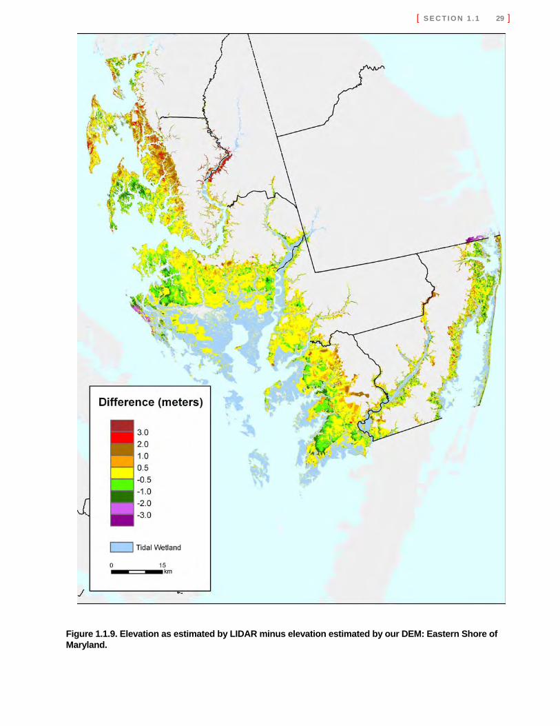
[ S E C T I O N 1 . 1 29 ]

Figure 1.1.9. Elevation as estimated by LIDAR minus elevation estimated by our DEM: Eastern Shore of Maryland.

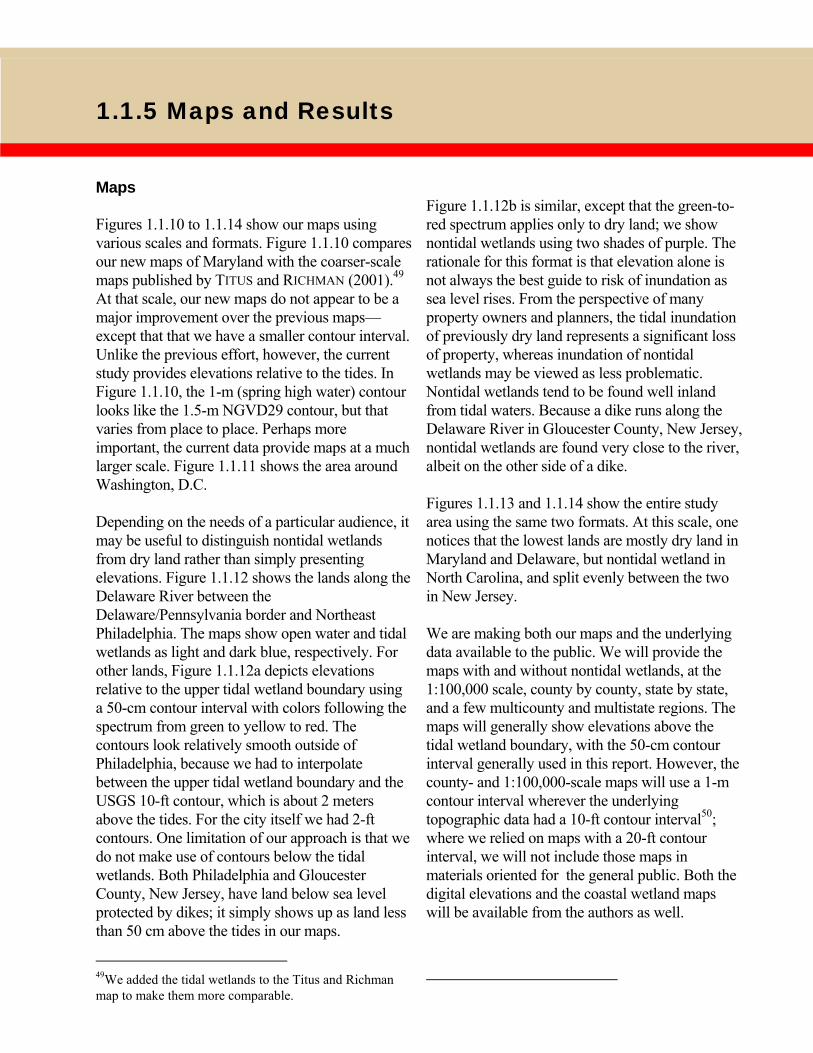
Maps Figures 1.1.10 to 1.1.14 show our maps using various scales and formats. Figure 1.1.10 compares our new maps of Maryland with the coarser-scale maps published by TITUS and RICHMAN (2001).49 At that scale, our new maps do not appear to be a major improvement over the previous maps—except that that we have a smaller contour interval. Unlike the previous effort, however, the current study provides elevations relative to the tides. In Figure 1.1.10, the 1-m (spring high water) contour looks like the 1.5-m NGVD29 contour, but that varies from place to place. Perhaps more important, the current data provide maps at a much larger scale. Figure 1.1.11 shows the area around Washington, D.C. Depending on the needs of a particular audience, it may be useful to distinguish nontidal wetlands from dry land rather than simply presenting elevations. Figure 1.1.12 shows the lands along the Delaware River between the Delaware/Pennsylvania border and Northeast Philadelphia. The maps show open water and tidal wetlands as light and dark blue, respectively. For other lands, Figure 1.1.12a depicts elevations relative to the upper tidal wetland boundary using a 50-cm contour interval with colors following the spectrum from green to yellow to red. The contours look relatively smooth outside of Philadelphia, because we had to interpolate between the upper tidal wetland boundary and the USGS 10-ft contour, which is about 2 meters above the tides. For the city itself we had 2-ft contours. One limitation of our approach is that we do not make use of contours below the tidal wetlands. Both Philadelphia and Gloucester County, New Jersey, have land below sea level protected by dikes; it simply shows up as land less than 50 cm above the tides in our maps.

49We added the tidal wetlands to the Titus and Richman map to make them more comparable.

Figure 1.1.12b is similar, except that the green-to-red spectrum applies only to dry land; we show nontidal wetlands using two shades of purple. The rationale for this format is that elevation alone is not always the best guide to risk of inundation as sea level rises. From the perspective of many property owners and planners, the tidal inundation of previously dry land represents a significant loss of property, whereas inundation of nontidal wetlands may be viewed as less problematic. Nontidal wetlands tend to be found well inland from tidal waters. Because a dike runs along the Delaware River in Gloucester County, New Jersey, nontidal wetlands are found very close to the river, albeit on the other side of a dike. Figures 1.1.13 and 1.1.14 show the entire study area using the same two formats. At this scale, one notices that the lowest lands are mostly dry land in Maryland and Delaware, but nontidal wetland in North Carolina, and split evenly between the two in New Jersey. We are making both our maps and the underlying data available to the public. We will provide the maps with and without nontidal wetlands, at the 1:100,000 scale, county by county, state by state, and a few multicounty and multistate regions. The maps will generally show elevations above the tidal wetland boundary, with the 50-cm contour interval generally used in this report. However, the county- and 1:100,000-scale maps will use a 1-m contour interval wherever the underlying topographic data had a 10-ft contour interval50; where we relied on maps with a 20-ft contour interval, we will not include those maps in materials oriented for the general public. Both the digital elevations and the coastal wetland maps will be available from the authors as well.

1.1.5 Maps and Results

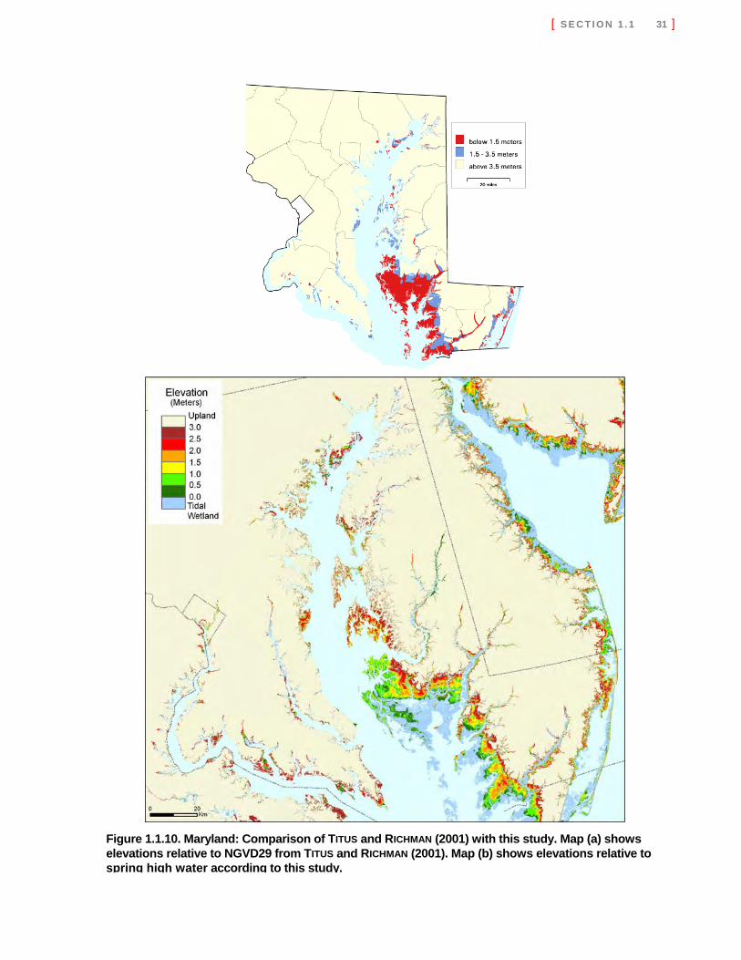
[ S E C T I O N 1 . 1 31 ]

Figure 1.1.10. Maryland: Comparison of TITUS and RICHMAN (2001) with this study. Map (a) shows elevations relative to NGVD29 from TITUS and RICHMAN (2001). Map (b) shows elevations relative to spring high water according to this study.

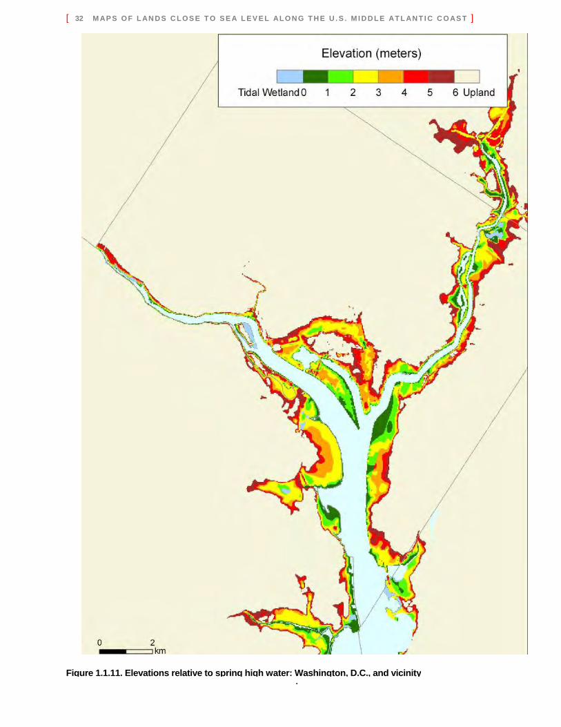
[ 32 M AP S O F L AN D S C L O S E T O S E A L E V E L AL O N G T H E U . S . M I D D L E AT L AN T I C C O AS T ]

.

Figure 1.1.11. Elevations relative to spring high water: Washington, D.C., and vicinity

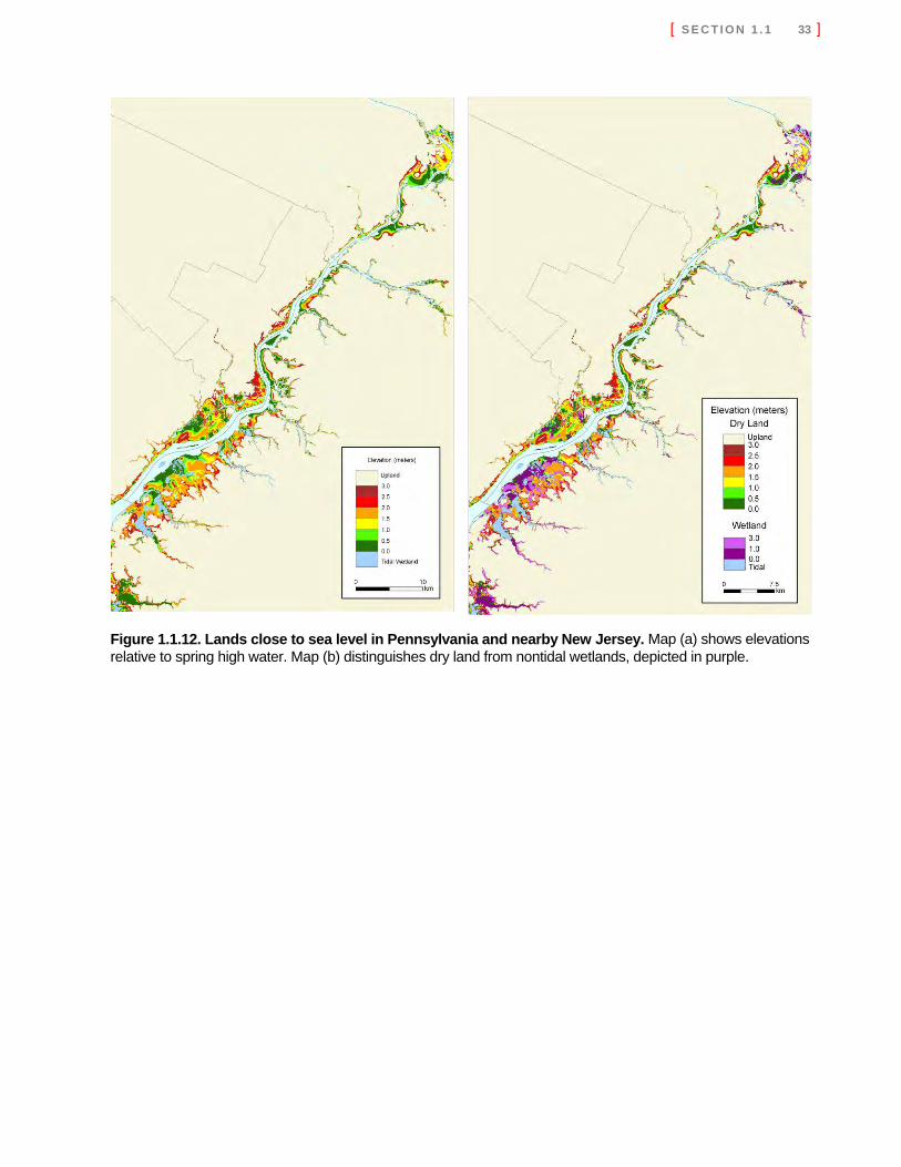
[ S E C T I O N 1 . 1 33 ]

Figure 1.1.12. Lands close to sea level in Pennsylvania and nearby New Jersey. Map (a) shows elevations relative to spring high water. Map (b) distinguishes dry land from nontidal wetlands, depicted in purple.

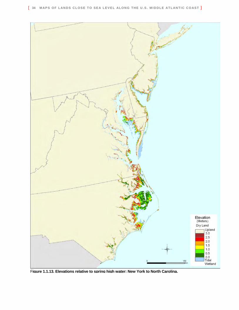
[ 34 M AP S O F L AN D S C L O S E T O S E A L E V E L AL O N G T H E U . S . M I D D L E AT L AN T I C C O AS T ]

Figure 1.1.13. Elevations relative to spring high water: New York to North Carolina.

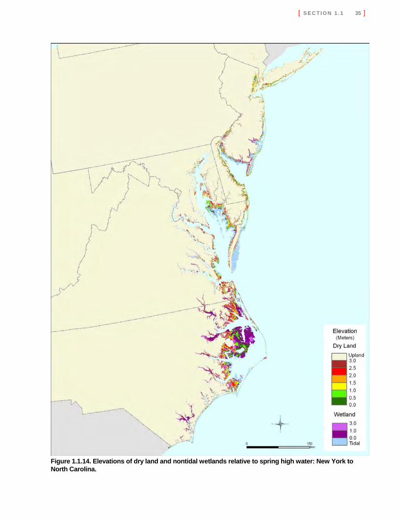
[ S E C T I O N 1 . 1 35 ]

Figure 1.1.14. Elevations of dry land and nontidal wetlands relative to spring high water: New York to North Carolina.

[ 36 M AP S O F L AN D S C L O S E T O S E A L E V E L AL O N G T H E U . S . M I D D L E AT L AN T I C C O AS T ]

Results Tables 1.1.5 and 1.1.6 provide our estimates of the land within 6 meters above spring high water, in 50-cm elevation increments. Although the maps show that the distribution of elevations varies from place to place, Table 1.1.5 shows that at the statewide level, the amount of dry land at various elevations is fairly uniform. Previous studies that were forced to rely on 5-m contour intervals and assume that the dry land below 1 meter is one-fifth that amount, for example, appear to have made a reasonable assumption. For the most part, the amount of dry land within 1 meter of high water is within 25 percent of the amount of land between 4 and 5 meters. Given the various geological processes that cause land to form just above sea level, it is not surprising that that area of land within 1 meter would be slightly greater than the area between 4 and 5 meters. At first glance, North Carolina appears to be an important exception to this tendency, with less land below 50 cm than at other elevation increments. At most of the elevations depicted, North Carolina has 500–700 km2, almost as much as the 600–800 km2 for the other seven states combined. Below 50 cm, however, North Carolina has only approximately 100 km2 of dry land. Table 1.1.6 (and Figure 1.1.14) shows why: close to 2,000 km2 of nontidal wetlands. Looking at all lands above the tides, North Carolina has about 2,000 km2 between 0 and 50 cm, 1,400 km2

between 50 and 100 cm, and 800–900 km2 for each of the other 50-cm increments below 5 meters. Thus, considering Tables 1.1.5 and 1.1.6 together gives us the opposite picture as Table 1.1.5 alone: more land between 0 and 1 meters than between 1 and 2 meters and other elevation increments. That result, however, is probably an artifact of the definition of tidal wetlands. As we have discussed, the nanotidal wetlands of Albemarle and Pamlico sounds and their tributaries are generally classified as nontidal wetlands. These wetlands depend on sea level, however, as much as most tidal wetlands: their vertical accretion is in part a function of sea level rise. The nontidal wetlands may be vulnerable to sea level rise as well: their irregular flooding tends to occur either from high water levels in the sounds or because of a combination of rainfall and the very slow drainage

that results from being barely above sea level. Agricultural and other dry lands just above these nontidal wetlands could become wet if the sea rose, just as lands above tidal wetlands can be inundated as sea level rises. Thus, it is somewhat misleading to classify those wetlands with other nontidal wetlands in an analysis of sea level rise. As Table 1.1.6 shows, North Carolina is unique in that its area of nontidal wetlands below 50 cm is greater than the area of tidal wetlands; the remaining states, by contrast, have about 20 times as much tidal wetlands as nontidal wetlands below 50 cm. Tables 1.1.5 and 1.1.6 also support previous assessments suggesting a potential for a significant net loss of wetlands if sea level rise accelerates. This report focuses solely on the topographic vulnerability of wetlands, that is, the ratio of current tidal wetlands to the area of low land that could potentially become inundated. Companion studies are examining the potential for vertical accretion and the extent to which shore protection might thwart landward migration. From New York to Virginia, the area of dry land within 1 meter above the tides is only about one-fourth the current area of tidal wetlands. North Carolina has approximately 3,000 km2 of wetlands less than 50 cm above the tides, but only 700 km2 of dry land within 1 meter above the tides. Figure 1.1.15 shows county-by-county variability of the ratio of tidal wetlands to dry land within 1 meter above the tides.51 Because 1 meter is somewhat arbitrary, Figure 1.1.15b shows a similar ratio, but with the area of land within one-half the tide range (instead of 1 meter) above spring high water in the denominator. This ratio indicates the net loss of tidal wetlands that would occur if sea level were to rise one-half the tide range instantaneously. (We exclude North Carolina because the small tide range would give us a meaninglessly large ratio.) Equivalently, this figure shows the ratio of the average slope immediately above spring high water to the average slope between spring high water and the open water. Across the region depicted, the average ratio is about eight. That is, if wetlands were able to migrate inland unfettered by 51Counties that are partly along the ocean and partly along Chesapeake Bay, Delaware Bay, or Long Island Sound are split.

[ S E C T I O N 1 . 1 37 ]

shore protection, but were not able to vertically accrete, sea level rise would eventually cause the area of tidal wetlands to decline by 7/8. Thus, the fate of tidal wetlands in the mid-Atlantic is likely to depend more on their ability to accrete vertically than to migrate inland. The potential for wetlands to keep pace with an accelerated rise is sea level uncertain (see Reed et al., Section 2.1 of this report). A priority for additional research would thus be to determine whether human activities are impairing—and how they might be able to enhance—the ability of wetlands to keep pace with rising sea level. Comparison with Comparable Studies Two previous mapping studies funded by the EPA assessed the amount of mid-Atlantic land vulnerable to sea level rise. TITUS and RICHMAN (2001) reported results only for the 1.5 and 3.5 contours, relative to NGVD29, without distinguishing wet from dry land, for each state in the Atlantic and Gulf coasts. Table 1.1.7 compares our results to their results for the eight Mid-Atlantic states. For both elevation increments, this analysis finds more low land than the previous effort for every state except North Carolina. In fact, for the seven states from New York to Virginia, our estimate of tidal wetlands alone is greater than the previous estimate of land below 1.5 m. Because the 2001 study was largely based on the USGS 1° (1:250,000 scale) maps, our results are almost certainly more accurate. Our primary reliance on 5- and 10-ft contour intervals—as well as the coarse (30-m) cell size—suggests that comparable (or greater) improvements are likely whenever this assessment can be revised using LIDAR. Finally, Table 1.1.8 compares our results to that of EPA’s 1989 Report to Congress, which remains the sole nationwide estimate of the land vulnerable to a 50- or 100-cm rise in sea level (PARK et al. 1989; TITUS and GREENE 1989). That study was primarily designed to estimate the vulnerability to a 2-m global rise in sea level, for which the available elevation maps seemed adequate. The need for an assessment of the more likely and near-term scenarios led the authors to interpolate

elevations below the contours, primarily using triangular irregular networks. PARK et al. included a dynamic model of how wetlands respond to sea level and provided land loss in 5-year increments, based on 48 sites equally dispersed around the nation representing 10 percent of the coastal 7.5-minute quads. Like this effort, that study used wetlands data to distinguish dry land and defined elevations using the USGS 7.5 minute quads—but the cell size was 500 meters. The Report to Congress (TITUS and GREENE 1989) grouped the sites into seven regions, so that confidence intervals could (barely) be developed to capture uncertainty regarding the extent to which the sample sites were representative of the coastal zone; the mid-Atlantic region was defined as New York to Virginia. The authors of the Report to Congress no longer have the intermediate results, so our only available comparison is the aggregate land loss for New York to Virginia. As Table 1.1.8 shows, our estimate of the land vulnerable to a 2-m rise is about 30 percent less than the estimate52 from the Report to Congress. Our estimates of the land vulnerable to a 50- or 100-cm rise, however, are 50-60 percent less than those of the 1989 study. The key difference is that our newer data suggest that that dry land is close to uniformly distributed by elevation below 5 meters,53 although PARK et al. found the dry land to be disproportionately close to sea level. As the final column shows, the Report to Congress, in effect, estimated land to be 30–40 cm lower on average than this study. Does our downward revision for the mid-Atlantic imply that the Report to Congress also overestimated the nationwide loss of land vulnerable to a 50-cm rise by a factor of three? Probably not: only three of the regions showed such a disproportionate amount of low land in the 1989 study. Moreover, the Report to Congress was based on a nationwide sample of 48 sites, only 8 of 52The Report to Congress did not report a confidence range for the regional estimates of dry land loss because the central estimates were less than two times the standard deviation. 53Of course, our results assume linearity between contours—but Tables 1.1.6 and 1.1.7 show elevations to be fairly uniform from contour interval to contour interval as well. Our areas with spot elevation data and LIDAR also show a fairly constant pattern.

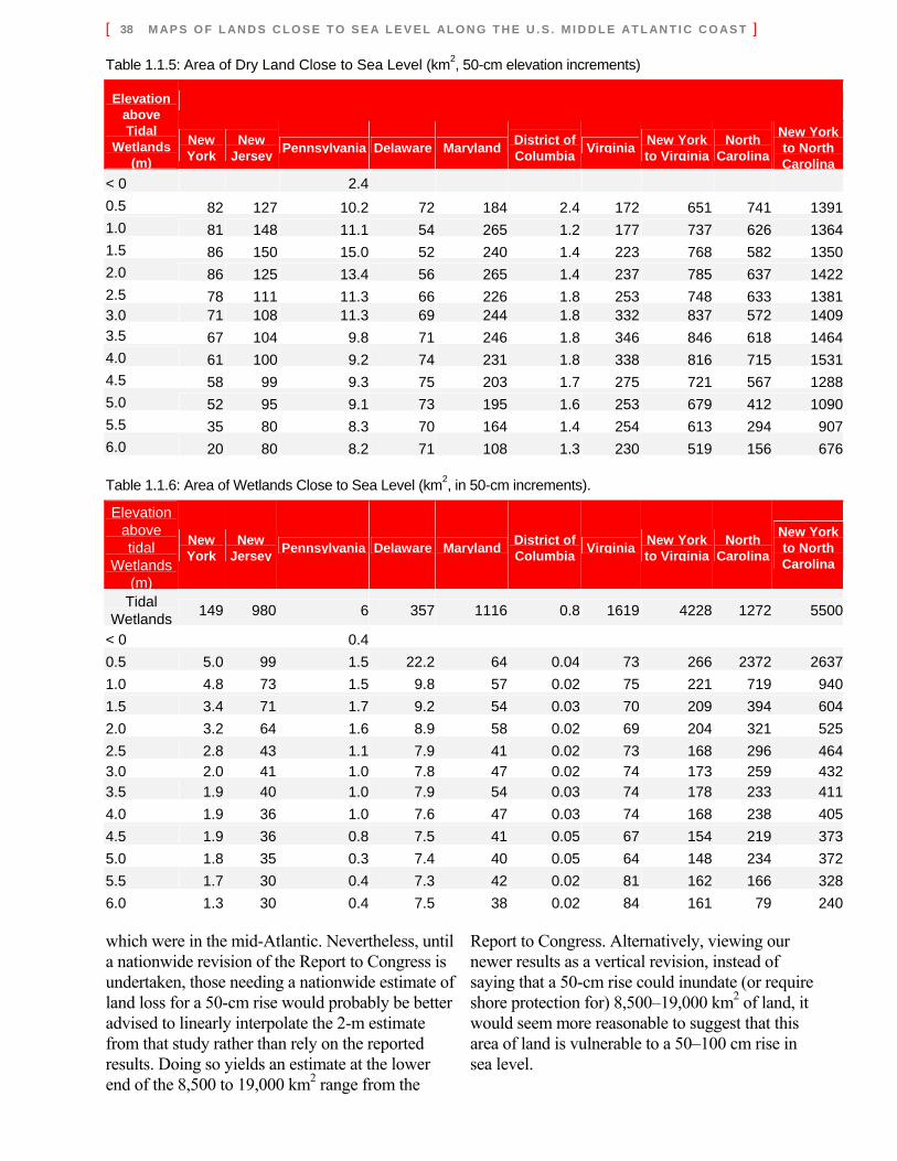
[ 38 M AP S O F L AN D S C L O S E T O S E A L E V E L AL O N G T H E U . S . M I D D L E AT L AN T I C C O AS T ]

which were in the mid-Atlantic. Nevertheless, until a nationwide revision of the Report to Congress is undertaken, those needing a nationwide estimate of land loss for a 50-cm rise would probably be better advised to linearly interpolate the 2-m estimate from that study rather than rely on the reported results. Doing so yields an estimate at the lower end of the 8,500 to 19,000 km2 range from the

Report to Congress. Alternatively, viewing our newer results as a vertical revision, instead of saying that a 50-cm rise could inundate (or require shore protection for) 8,500–19,000 km2 of land, it would seem more reasonable to suggest that this area of land is vulnerable to a 50–100 cm rise in sea level.

Table 1.1.5: Area of Dry Land Close to Sea Level (km2, 50-cm elevation increments)

Elevation above Tidal

Wetlands (m)

New York

New Jersey Pennsylvania Delaware Maryland District of

Columbia Virginia New York to Virginia

North Carolina

New York to North Carolina

< 0 2.4 0.5 82 127 10.2 72 184 2.4 172 651 741 13911.0 81 148 11.1 54 265 1.2 177 737 626 13641.5 86 150 15.0 52 240 1.4 223 768 582 13502.0 86 125 13.4 56 265 1.4 237 785 637 14222.5 78 111 11.3 66 226 1.8 253 748 633 13813.0 71 108 11.3 69 244 1.8 332 837 572 14093.5 67 104 9.8 71 246 1.8 346 846 618 14644.0 61 100 9.2 74 231 1.8 338 816 715 15314.5 58 99 9.3 75 203 1.7 275 721 567 12885.0 52 95 9.1 73 195 1.6 253 679 412 10905.5 35 80 8.3 70 164 1.4 254 613 294 9076.0 20 80 8.2 71 108 1.3 230 519 156 676 Table 1.1.6: Area of Wetlands Close to Sea Level (km2, in 50-cm increments).

Elevation above tidal

Wetlands (m)

New York

New Jersey Pennsylvania Delaware Maryland District of

Columbia Virginia New York to Virginia

North Carolina

New York to North Carolina

Tidal Wetlands 149 980 6 357 1116 0.8 1619 4228 1272 5500

< 0 0.4 0.5 5.0 99 1.5 22.2 64 0.04 73 266 2372 26371.0 4.8 73 1.5 9.8 57 0.02 75 221 719 9401.5 3.4 71 1.7 9.2 54 0.03 70 209 394 6042.0 3.2 64 1.6 8.9 58 0.02 69 204 321 5252.5 2.8 43 1.1 7.9 41 0.02 73 168 296 4643.0 2.0 41 1.0 7.8 47 0.02 74 173 259 4323.5 1.9 40 1.0 7.9 54 0.03 74 178 233 4114.0 1.9 36 1.0 7.6 47 0.03 74 168 238 4054.5 1.9 36 0.8 7.5 41 0.05 67 154 219 3735.0 1.8 35 0.3 7.4 40 0.05 64 148 234 3725.5 1.7 30 0.4 7.3 42 0.02 81 162 166 3286.0 1.3 30 0.4 7.5 38 0.02 84 161 79 240

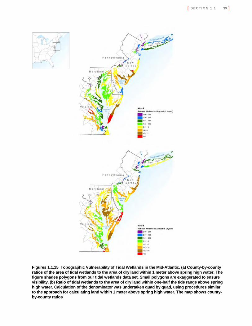
[ S E C T I O N 1 . 1 39 ]

Figures 1.1.15 Topographic Vulnerability of Tidal Wetlands in the Mid-Atlantic. (a) County-by-county ratios of the area of tidal wetlands to the area of dry land within 1 meter above spring high water. The figure shades polygons from our tidal wetlands data set. Small polygons are exaggerated to ensure visibility. (b) Ratio of tidal wetlands to the area of dry land within one-half the tide range above spring high water. Calculation of the denominator was undertaken quad by quad, using procedures similar to the approach for calculating land within 1 meter above spring high water. The map shows county-by-county ratios

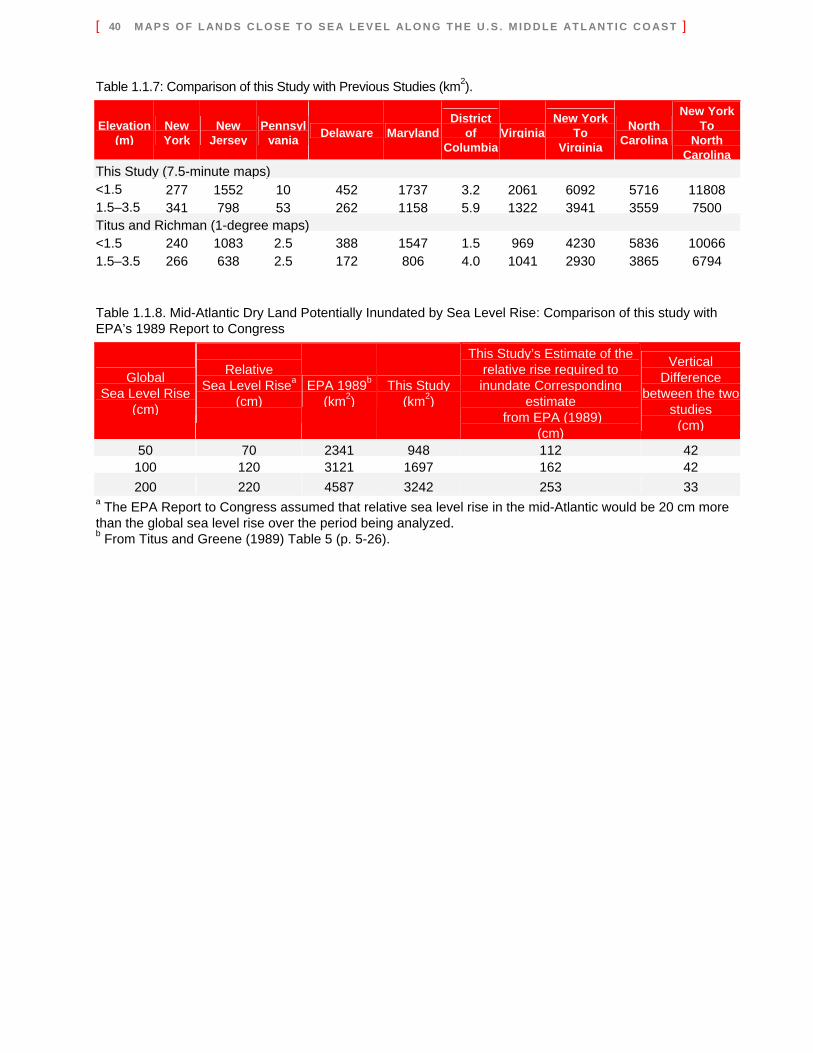
[ 40 M AP S O F L AN D S C L O S E T O S E A L E V E L AL O N G T H E U . S . M I D D L E AT L AN T I C C O AS T ]

Table 1.1.8. Mid-Atlantic Dry Land Potentially Inundated by Sea Level Rise: Comparison of this study with EPA’s 1989 Report to Congress

Global Sea Level Rise

(cm)

Relative

Sea Level Risea (cm)

EPA 1989b (km2)

This Study (km2)

This Study’s Estimate of the relative rise required to inundate Corresponding

estimate from EPA (1989)

(cm)

Vertical Difference

between the two studies

(cm)

50 70 2341 948 112 42 100 120 3121 1697 162 42 200 220 4587 3242 253 33

a The EPA Report to Congress assumed that relative sea level rise in the mid-Atlantic would be 20 cm more than the global sea level rise over the period being analyzed. b From Titus and Greene (1989) Table 5 (p. 5-26).

Table 1.1.7: Comparison of this Study with Previous Studies (km2).

Elevation (m)

New York

New Jersey

Pennsylvania Delaware Maryland

District of

ColumbiaVirginia

New York To

Virginia

North Carolina

New YorkTo

North Carolina

This Study (7.5-minute maps) <1.5 277 1552 10 452 1737 3.2 2061 6092 5716 11808 1.5–3.5 341 798 53 262 1158 5.9 1322 3941 3559 7500 Titus and Richman (1-degree maps) <1.5 240 1083 2.5 388 1547 1.5 969 4230 5836 10066 1.5–3.5 266 638 2.5 172 806 4.0 1041 2930 3865 6794

BARTH, M.C., AND J.G. TITUS. 1984. Greenhouse Effect and Sea Level Rise: A Challenge for this Generation. Van Nostrand Reinhold, New York.

BRUUN, P. 1962. Sea level rise as a cause of shore erosion. Journal of Waterways and Harbors Division (ASCE) 88: 116–130.

BUREAU OF THE BUDGET. 1947. National Map Accuracy Standards. Government Printing Office, Washington DC. http://rockyweb.cr.usgs.gov/nmpstds/nmas.html. (cited October 1 2006).

CAHOON, D.R., D.J. REED, and J.W. DAY. 1995. Estimating shallow subsidence in microtidal salt marshes of the southeastern United States: Kaye and Barghoorn revisited. Marine Geology 128: 1–9.

CHILDS, C. 2004. Interpolating surfaces in ArcGIS Spatial Analyst. ArcUser July-September: 32–35.

CHURCH, J.A., and N.J. WHITE. 2006. A 20th century acceleration in global sea-level rise. Geophysical Research Letters 33, L01602, doi:10.1029/2005GL024826.

COWELL, P.J., and B.G. THOM. 1994. Morphodynamics of coastal evolution. In Coastal Evolution. R.W.G. CARTER and C.D. WOODROFFE (eds.). Cambridge University Press, Cambridge, U.K. and New York, pp. 33-86.

COWELL, P.J., P.S. ROY, and R.A. JONES. 1995. Simulation of large-scale coastal change using a morphological behavior model. Marine Geology 126: 45–61.

DEAN, C. 2006. Next victim of warming: The beaches. New York Times (Science Times). pp. D1, D4. January 20.

DEAN, R.G., and E.M. MAURMEYER. 1983. Models of beach profile response. In CRC Handbook of Coastal Processes and Erosion, P. KOMAR and J. MOORE (eds.). CRC Press, Boca Raton, FL: pp. 151–165.

ESRI. 1998. ARC/INFO, 7.2.1 edition. Environmental Systems Research Institute, Redlands, CA.

FEDERAL GEODETIC CONTROL SUBCOMMITTEE, FEDERAL GEOGRAPHIC DATA COMMITTEE. 1998. Geospatial Positioning Accuracy Standards. Report FGDC-STD-007.1-1998. Washington, DC.

FISHER, N.I., T. LEWIS, and B.J.J. EMBLETON. 1987. Statistical Analysis of Spherical Data. Cambridge University Press, Cambridge, U.K.

FREY, R.W., and P.B. BASAN. 1985. Coastal salt marshes. In: Coastal Sedimentary Environments, R.S. Davis (ed.). Springer-Verlag, New York, p. 225-301.

GILL, S.K., and J.R. SCHULTZ (eds.). 2001. Tidal Datums and Their Applications. National Ocean Service, Silver Spring, MD.

HICKS, S.D., H.A. DEBAUGH, and L.H. HICKMAN, 1983. Sea Level Variations for the United States 1855–1980. U.S. Department of Commerce, National Ocean Service, Rockville, MD.

Literature Cited

[ 42 M AP S O F L AN D S C L O S E T O S E A L E V E L AL O N G T H E U . S . M I D D L E AT L AN T I C C O AS T ]

HUTCHINSON, M.F. 1988. Calculation of hydrologically sound digital elevation models. In Third International Symposium on Spatial Data Handling, Sydney. International Geographical Union, Columbus, OH, pp. 117-133.

HUTCHINSON, M.F. 1989. A new procedure for gridding elevation and stream line data with automatic removal of spurious pits. Journal of Hydrology 106: 211–232.

INTERAGENCY PERFORMANCE EVALUATION TASKFORCE. 2006. Performance Evaluation of the New Orleans and Southeast Louisiana Hurricane Protection System. U.S. Army Corps of Engineers, Washington, DC.

IPCC [INTERGOVERNMENTAL PANEL ON CLIMATE CHANGE]. 1996. Climate Change 1995: The Science of Climate Change. Cambridge University Press, New York.

IPCC [INTERGOVERNMENTAL PANEL ON CLIMATE CHANGE]. 2001a. Climate Change 2001: The Scientific Basis. Cambridge University Press, New York.

IPCC [INTERGOVERNMENTAL PANEL ON CLIMATE CHANGE]. 2001b. Climate Change 2001: Impacts, Adaptation, and Vulnerability. Cambridge University Press, New York.

IPCC [INTERGOVERNMENTAL PANEL ON CLIMATE CHANGE]. 2007. Climate Change 2007: The Physical Science Basis. Cambridge University Press, New York.

JONES, R. 2007. Accuracy Assessment of EPA Digital Elevation Model Results. Memorandum and attached spreadsheets prepared for the U.S. EPA under Work Assignment 409 of EPA Contract #68-W-02-027.

KANA, T.W., B.J. BACA, and M.L. WILLIAMS. 1988. Charleston case study. In Greenhouse Effect, Sea Level Rise, and Coastal Wetlands, J.G. Titus (ed.). U.S. EPA, Washington, DC.

KRISTOF, N.D. 2005. The storm next time. New York Times Section 4, Page 15, Column 6. (Sept. 11).

MD DNR [MARYLAND DEPARTMENT OF NATURAL RESOURCES]. 2004. LIDAR 2004 Gridded DEM. Department of Natural Resources, Annapolis.

MYERS, E.P. 2005. Review of progress on VDatum, a vertical datum transformation tool. Marine Technology Society/IEEE OCEANS Conference, Washington, DC., September 19-23.

NATIONAL GEODETIC SURVEY, DEWBERRY AND DAVIS, and PSOMAS & ASSOCIATES. 1998. Report to Congress: National Height Modernization Study. National Ocean Service, Silver Spring, MD.

NOS [NATIONAL OCEAN SERVICE]. 2000. Tides and Current Glossary. National Oceanic and Atmospheric Administration, National Ocean Service, Silver Spring, Maryland.

NOS [NATIONAL OCEAN SERVICE]. 2004. Tide Tables 2004. National Oceanic and Atmospheric Administration, National Ocean Service http://co-ops.nos.noaa.gov/tides04/tpred2.html, accessed October 1, 2007.

NOS [NATIONAL OCEAN SERVICE]. 2005. Published Benchmark Sheets. National Oceanic and Atmospheric Administration, National Ocean Service. http://co-ops.nos.noaa.gov/bench.html, accessed May 1, 2005.

NRC [NATIONAL RESEARCH COUNCIL, MARINE BOARD]. 1987. Responding to Changes in Sea Level. National Academy Press, Washington, DC.

[ S E C T I O N 1 . 1 43 ]

OLSEN, L.M., and N.B. BLISS. 1997. Development of a 30-arc-second digital elevation model of South America. User Conference Proceedings: 1997 ESRI International User Conference (July 8–11). ESRI, San Diego, CA.

PARK, R.A., M.S. TREEHAN, P.W. MAUSEL, and R.C. HOWE. 1989. The effects of sea level rise on U.S. coastal wetlands. In Potential Effects of Global Climate Change on the United States. U.S. EPA, Washington, DC.

PARKER, B., K.W. HESS, D.G. MILBERT, and S. GILL. 2003. National V-Datum: The implementation of a national vertical datum transformation database. U.S. Hydrographic Conference, Biloxi, MS, March 24-27.

PERMANENT SERVICE FOR MEAN SEA LEVEL. 2003. Some Example Applications of the Use of PSMSL Data: A Table of Long-Term Trends. Proudman Oceanographic Laboratory, Liverpool, United Kingdom.

PILKEY, O., J. HOWARD, B. BRENNINKMEYER, R. FREY, A. HINE, J. KRAFT, R. MORTON, D. NUMMEDAL, and H. WANLESS. 1982. Saving the American beach: A position paper by concerned coastal geologists. Results of the Skidaway Institute of Oceanography conference on America's eroding shoreline. Shore and Beach 2 (April): 3–8.

PRICE, M. 1999. Terrain modeling with ArcView 3D analyst. ArcUser January-March. http://www.esri.com/news/arcuser/0199/web4.html (accessed July 1, 2006).

REIMOLD, R.J. 1977. Mangals and salt marshes of eastern United States. In Ecosystems of the World. 1. Wet Coastal Ecosystems, V.J. Chapman (ed.). Elsevier Scientific Publishing Company, New York, pp. 157-166.

ROGERS, D.F., and S.G. SATTERFIELD. 1980. B-Spline curves and surfaces for ship hull design. Computer Graphics Quarterly 14(3): 211–217.

SCHNEIDER, S.H., and R.S. CHEN. 1980. Carbon dioxide flooding: Physical factors and climatic impact. Annual Review of Energy 5: 107–140.

SHEPARD, D. 1968. A two-dimensional interpolation function for irregularly-spaced data. Proceedings of the 23rd National Conference (ACM), pp. 517–524.

See http://portal.acm.org/citation.cfm?id=810616 or http://portal.acm.org/ft_gateway.cfm?id=810616&type=pdf or google report title.

SLADE, D.C., R.K. KEHOE, and M.M. FLEMING. 1990. Lands, waters and living resources subject to the public trust doctrine. In Putting the Public Trust Doctrine to Work, D.C. Slade, (ed.). Coastal States Organization, Washington DC, pp. 13-128

STOUT, J.P. 1988. Irregularly flooded salt marshes of the Gulf and Atlantic Coasts of the United States. In The Ecology and Management of Wetlands Volume 1: Ecology of Wetlands, D.D. Hook, W.H. McKee, Jr., H.K. Smith, J. Gregory, V.G. Burrell, Jr., M.R. DeVoe, R.E. Sojka, S. Gilbert, R. Banks, L.H. Stolzy, C. Brooks, T.D. Matthews, and T.H. Shear (eds.). Timber Press, Portland, OR, pp. 511-525.

TEAL, J., and M. TEAL. 1969. Life and Death of the Salt Marsh. Ballantine Books, New York.

[ 44 M AP S O F L AN D S C L O S E T O S E A L E V E L AL O N G T H E U . S . M I D D L E AT L AN T I C C O AS T ]

TITUS, J.G. 1990. Greenhouse effect, sea level rise, and barrier islands: Case study of Long Beach Island, New Jersey. Coastal Management 18:65-90.

TITUS, J.G. 1998. Rising seas, coastal erosion, and the takings clause: How to save wetlands and beaches without hurting property owners. Maryland Law Review 57: 1279-1399.

TITUS, J.G. 2004. Maps that depict the business-as-usual response to sea level rise in the decentralized United States of America. In Global Forum on Sustainable Development: Development and Climate Change. Paris, 11-12 November 2004. Organization of Economic Cooperation and Development. As of January 1, 2007, available at http://www.oecd.org/document/60/0,2340,en_2649_34361_33868732_1_1_1_1,00.html.

TITUS, J.G., and M. GREENE. 1989. An overview of the nationwide impacts of sea level rise. In Report to Congress: Potential Impacts of Global Climate Change on the United States. U.S. EPA, Washington, DC.

TITUS, J.G., and V. NARAYANAN. 1996. The risk of sea level rise: A Delphic Monte Carlo analysis in which twenty researchers specify subjective probability distributions for model coefficients within their respective areas of expertise. Climatic Change 33: 151-212.

TITUS, J.G., and C. RICHMAN. 2001. Maps of lands vulnerable to sea level rise: Modeled elevations along the U.S. Atlantic and Gulf coasts. Climate Research 18:205-228.

U.S. EPA [U.S. ENVIRONMENTAL PROTECTION AGENCY]. 1996. The Probability of Sea Level Rise. Climate Change Division, Washington, DC.

U.S. EPA [U.S. ENVIRONMENTAL PROTECTION AGENCY] and U.S. ARMY CORPS OF ENGINEERS. 1990. Mitigation Memorandum of Agreement (Feb. 6). U.S. EPA and U.S. Army Corps of Engineers, Washington, DC.

US CLIMATE CHANGE RESEARCH PROGRAM. 2003. Strategic Plan for the U.S. Climate Change Science Program. National Oceanic and Atmospheric Administration, Washington, DC.

YOUNG, R.S., and O.H. PILKEY. 1995. A discussion of the generalized model for simulating shoreline changes (GENESIS). Journal of Coastal Research 11(3): 875–886.

WEISS, J.L., and J.T. OVERPECK. 2006. Climate Change and Sea Level: Maps of Susceptible Areas. Department of Geosciences, University of Arizona. Available at http://www.geo.arizona.edu/dgesl/index.html" as of January 12, 2007.

WILLIAMS, S.J., K. DODD, and K.K. GOHN. 1995. Coasts in Crisis. U.S. Geological Survey Circular 1075. U.S. Geological Survey, Washington, DC.

ZERVAS, C.E. 2001. Sea Level Variations of the United States 1854–1999. NOAA Technical Report NOS CO-OPS 36, National Oceanic and Atmospheric Administration, Silver Spring, MD.