ARTICLE

Mapping the Wind Hazard of Global Tropical Cycloneswith Parametric Wind Field Models by Considering the Effectsof Local Factors

Chenyan Tan1,2 • Weihua Fang1,2

Published online: 7 February 2018

� The Author(s) 2018. This article is an open access publication

Abstract Tropical cyclones (TCs) cause catastrophic loss

in many coastal areas of the world. TC wind hazard maps

can play an important role in disaster management. A good

representation of local factors reflecting the effects of

spatially heterogeneous terrain and land cover is critical to

evaluation of TC wind hazard. Very few studies, however,

provide global wind hazard assessment results that consider

detailed local effects. In this study, the wind fields of his-

torical TCs were simulated with parametric models in

which the planetary boundary layer models explicitly

integrate local effects at 1 km resolution. The topographic

effects for eight wind directions were quantified over four

types of terrain (ground, escarpment, ridge, and valley),

and the surface roughness lengths were estimated from a

global land cover map. The missing TC parameters in the

best track datasets were reconstructed with local regression

models. Finally, an example of a wind hazard map in the

form of wind speeds under a 100-year return period and

corresponding uncertainties was created based on a statis-

tical analysis of reconstructed historical wind fields over

seven of the world’s ocean basins.

Keywords Surface roughness � Topographiceffect � Tropical cyclone � Wind field model � Wind

hazard

1 Introduction

Tropical cyclones (TCs) cause casualties and enormous

economic losses in the coastal areas of the world (Guha-

Sapir et al. 2013). Annually, there are approximately 90

TCs globally (Knapp et al. 2010). Wind is one of the major

hazards of TCs, which not only brings direct property

damage but also determines the intensity of other sec-

ondary hazards, such as storm surge and waves.

Tropical cyclonic wind hazard is often quantified by the

statistical distribution of storm intensity and frequency and

is delineated in the form of a wind speed map of the return

period (Fang and Lin 2013). For a single site, the frequency

of wind speeds is usually analyzed with methods like the

extreme value theory (EVT), which is based on historical

ground meteorological observations (Elsner et al. 2008).

For local areas, ground observations might be insufficient

and modeling of historical or stochastic simulated TCs

based on the Monte-Carlo method (Russell 1969; Huang

et al. 2001) is needed. For larger areas, methods using

basin-wide stochastic simulations of full TC tracks have

been developed (Vickery et al. 2000; Emanuel et al. 2006).

A TC wind field can be simulated by numerical or

parametric methods. Although numerical models, such as

the Weather Research and Forecasting (WRF) model

(Skamarock et al. 2005; Nolan et al. 2009), have been

widely used in wind field reconstruction and forecasting,

parametric wind field models gained popularity in TC wind

hazard assessment for their satisfactory modeling accuracy

with limited TC parameters as inputs. Usually, the key

parameters can be obtained from historical TC track

datasets, and great efforts have been made to compile the

best tracks around the globe (Knapp et al. 2010). But

derived parameter values sometimes are of low reliability,

& Weihua Fang

weihua.fang@bnu.edu.cn

1 Key Laboratory of Environmental Change and Natural

Disaster of Ministry of Education, Faculty of Geographical

Science, Beijing Normal University, Beijing 100875, China

2 Academy of Disaster Reduction and Emergency

Management, Ministry of Civil Affairs and Ministry of

Education, Beijing Normal University, Beijing 100875,

China

123

Int J Disaster Risk Sci (2018) 9:86–99 www.ijdrs.com

https://doi.org/10.1007/s13753-018-0161-1 www.springer.com/13753

and the poor quality of TC parameters may influence the

reliability of parametric models.

Progress on TC wind hazard assessment displays great

regional disparity among countries and regions. At the

country level, wind hazard models have been developed

and widely applied in several TC-prone countries. For

example, in the United States, the HAZUS hurricane model

has been developed and improved since 1997 (FEMA

2012), and the Florida Office of Insurance Regulation has

supported the development of the Florida Public Hurricane

Loss Model (FIU 2011). In Central America, the Com-

prehensive Approach to Probabilistic Risk Assessment

(CAPRA) has been developed covering many countries

(Cardona et al. 2012), and, in Australia, the Tropical

Cyclone Risk Model (TCRM) was developed in 2008

(Arthur et al. 2008) and was released in 2011 (Summons

and Arthur 2011). At the global scale, the global historical

TC wind fields (1970–2010) were simulated in 2011 using

a parametric wind field model (Holland model) for all

basins around the world, which was supported by UNEP

(UNISDR 2009, 2011). Based on this study, global wind

speed maps at various return periods were derived (Giu-

liani and Peduzzi 2011), and the methods were slightly

improved in 2013 and 2015 (CIMNE 2013; UNISDR

2013, 2015).

A large gap still exists in the improvement of global

wind hazard assessment. In general, wind hazards are

spatially heterogeneous, and local factors, such as altitude,

slope and aspect, land use and land cover, greatly influence

wind profiles at the local scale (Lee et al. 2009; FEMA

2012). However, in most existing studies at the country or

global scale, the impact of local factors on TC wind haz-

ards is oversimplified or not considered (Vickery et al.

2000; Arthur et al. 2008; UNISDR

2009, 2011, 2013, 2015). The lack of observations of

important TC parameters (Knapp et al. 2010; Landsea and

Franklin 2013; Ying et al. 2014) also poses a great chal-

lenge to the modeling of wind fields. As a result, there are

few TC wind hazard products for the Northwest Pacific

(NWP), North Indian (NI), and South Indian (SI) basins

that are publicly available, although a few proprietary

models have been developed and released in the form of a

black box (FIU 2011).

The objective of this study is to map the TC wind hazard

at the global scale through parametric wind field models

selected for seven ocean basins, which is part of the overall

effort to map a variety of global disasters (Shi and

Kasperson 2015). The effects of local factors, including

topography and surface roughness, are modeled and dis-

cussed in detail in this article. Based on the simulated wind

fields with historical observed or reconstructed TC

parameters, the hazard maps are developed through a

statistical analysis of wind intensity and frequency that

considers uncertainty.

2 Datasets

The main datasets used in this study included the TC best

tracks observed by regional meteorological centers (Knapp

et al. 2010; Landsea and Franklin 2013; Ying et al. 2014).

In the datasets, TC parameters, including TC number, time

(year, month, day, and hour), locations (longitude and

latitude of TC center, lon and lat), central pressure (Pc),

maximum wind speed (Vm), and radius of maximum wind

speed (Rm), are archived at a time interval of 6 h. The

World Meteorological Organization (WMO) has been

integrating all TC best track datasets through the Interna-

tional Best Track Archive for Climate Stewardship

(IBTrACS) project (Knapp et al. 2010), which may pro-

duce inhomogeneities in both temporal and spatial

dimensions owing to different data sources (Levinson et al.

2010).

In this study, the TC best track dataset of seven ocean

basins are used. Following the quality comparison studies,

the China Meteorological Administration (CMA) best track

dataset (Ying et al. 2014) for the NWP, the U.S. National

Hurricane Center’s North Atlantic hurricane database

(HURDAT) (Landsea and Franklin 2013) for the North

Atlantic (NA), Northeast Pacific (NEP), and Central Pacific

(CP), and IBTrACS for the other three basins—NI, South

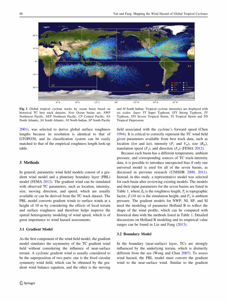
Pacific (SP), and SI, were adopted. The map of archived

historical TCs is shown in Fig. 1, and displays storm

intensity according to each storm’s maximum sustained

winds (SAC 2006). For NEP and CP, the TC tracks are

usually trans-boundary and cover both basins therefore the

two basins are treated as one unit for analysis, as shown in

Fig. 1. For South Atlantic (SA) basin, the genesis of TC is

very rare (Mctaggart-Cowan et al. 2006) and therefore SA

is excluded in this study.

A digital elevation model of the world is needed to

reflect the topographic effects on TC winds. In this study,

the 1 km GTOPO30 data (USGS 1996) were selected after

being compared with other freely available global digital

elevation model (DEM) products, such as the 90 m Shuttle

Radar Topography Mission (SRTM) (Jarvis et al. 2008)

and 30 m Global Digital Elevation Model (GDEM)

(ASTER GDEM Validation Team 2011). For wind field

modeling, 1 km is an appropriate resolution owing to the

computation resource requirements.

Another dataset for wind field modeling is land use or

land cover, which is used to estimate the surface roughness

length. In this study, the global land cover classification for

2000 version 2.0 (Loveland et al. 2000), which is based on

the USGS Land Use/Land Cover System Scheme (USGS

123

Int J Disaster Risk Sci 87

2001), was selected to derive global surface roughness

lengths because its resolution is identical to that of

GTOPO30, and its classification system can be easily

matched to that of the empirical roughness length look-up

table.

3 Methods

In general, parametric wind field models consist of a gra-

dient wind model and a planetary boundary layer (PBL)

model (FEMA 2012). The gradient wind can be simulated

with observed TC parameters, such as location, intensity,

size, moving direction, and speed, which are usually

available or can be derived from the TC track dataset. The

PBL model converts gradient winds to surface winds at a

height of 10 m by considering the effects of local terrain

and surface roughness and therefore helps improve the

spatial heterogeneity modeling of wind speed, which is of

great importance to wind hazard assessments.

3.1 Gradient Model

As the first component of the wind field model, the gradient

model simulates the asymmetry of the TC gradient wind

field without considering the influence of near-surface

terrain. A cyclonic gradient wind is usually considered to

be the superposition of two parts: one is the fixed circular

symmetry wind field, which can be obtained by the gra-

dient wind balance equation, and the other is the moving

field associated with the cyclone’s forward speed (Chen

1994). It is critical to correctly represent the TC wind field

given parameters available from best track data, such as

location (lon and lat), intensity (Pc and Vm), size (Rm),

translation speed (Fs), and direction (Fd) (FEMA 2012).

Because each basin has a different temperature, ambient

pressure, and corresponding sources of TC track-intensity

data, it is possible to introduce unexpected bias if only one

universal model is used for all of the seven basins, as

discussed in previous research (UNISDR 2009, 2011).

Instead, in this study, a representative model was selected

for each basin after reviewing existing models. The models

and their input parameters for the seven basins are listed in

Table 1, where Z0 is the roughness length, Tf is topographic

factor, Z (10 m) is the simulation height, and Pn is ambient

pressure. The gradient models for NWP, NI, SP, and SI

need the modeling of parameter Holland B to reflect the

shape of the wind profile, which can be computed with

historical data with the methods listed in Table 1. Detailed

discussions on Holland B modeling and its empirical value

ranges can be found in Lin and Fang (2013).

3.2 Boundary Model

In the boundary (near-surface) layer, TCs are strongly

influenced by the underlying terrain, which is distinctly

different from the sea (Wong and Chan 2007). To assess

wind hazard, the PBL model must convert the gradient

wind to the near-surface wind. Similar to the gradient

Fig. 1 Global tropical cyclone tracks by ocean basin based on

historical TC best track datasets. Note Ocean basins are: NWP

Northwest Pacific, NEP Northeast Pacific, CP Central Pacific, NA

North Atlantic, SA South Atlantic, NI North Indian, SP South Pacific

and SI South Indian. Tropical cyclone intensities are displayed with

six scales: Super TY Super Typhoon, STY Strong Typhoon, TY

Typhoon, STS Severe Tropical Storm, TS Tropical Storm and TD

Tropical Depression

123

88 Tan and Fang. Mapping the Wind Hazard of Global Tropical Cyclones

models, the PBL models for the seven basins were adopted

after reviewing existing studies.

The units used for TC sustained wind speeds may vary

by country, ranging from 1-, 2- to 10-min averages. In this

study, all sustained winds are converted into 3-s gust winds

according to a past study (ESDU 1983) because gust wind

is regarded to have the best statistical relationship with TC

damage.

In addition to the TC center (lon and lat), intensity (Pc

and Vm), and size (Rm), which are available in the best track

data, the other main input parameters of the PBL models

are terrain roughness (Z0) and topographic factors (Tf).

These parameters can be derived with digital elevation data

and land use/cover data.

3.2.1 Surface Roughness

The location of zero wind speed in the vertical wind pro-

file, which is defined as the aerodynamic roughness length

Z0 (Prigent et al. 2005), is not at the land surface but at a

certain height above the surface. According to the PBL

model (Meng et al. 1997) used in this study, the vertical

wind profile is given by

Uz ¼ Ug

z

zg

� �au

ð1Þ

where Uz is the wind speed at height z, Ug is the gradient

wind speed at the gradient layer height zg, and au is the

power law exponent for the wind speed profile. Both zg and

au are dependent on Z0 and therefore the surface wind

speed is heavily influenced by the value of Z0.

For small-scale studies, surface roughness can be

determined by direct field observations or wind tunnel tests

(Wieringa 1992). For large areas, roughness length is

usually estimated from land cover data determined from

remote sensing images (Silva et al. 2007; Ramli et al.

2009). Currently, there is no definite standard for

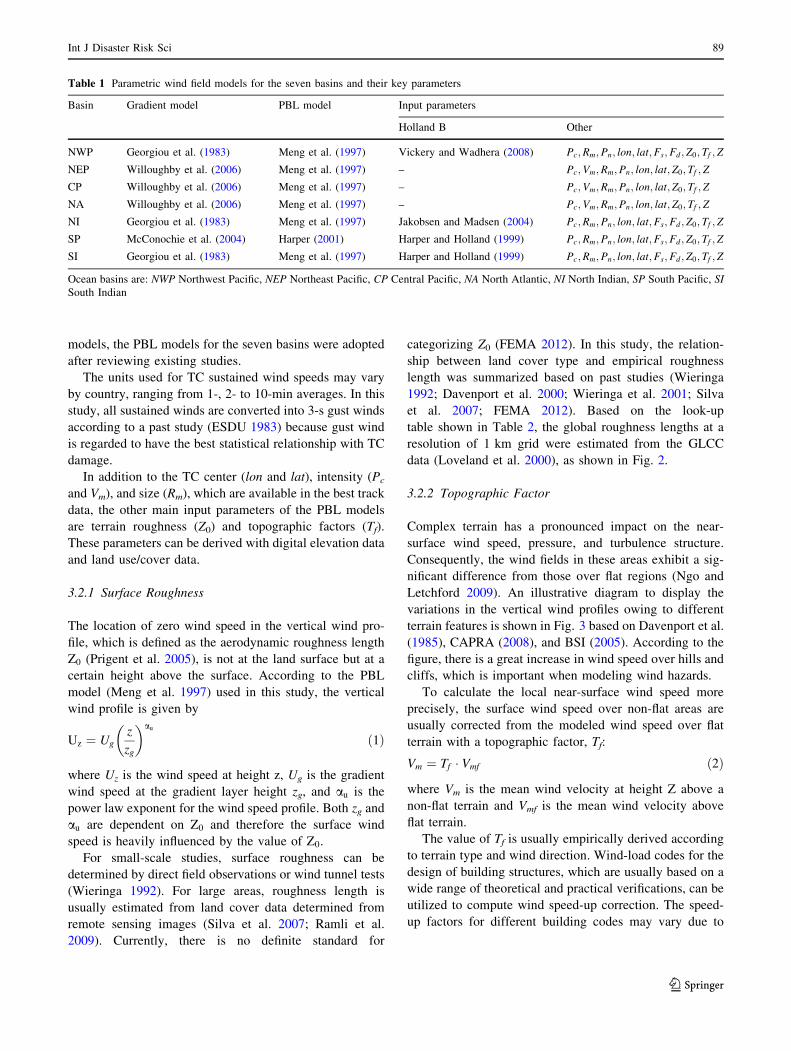
categorizing Z0 (FEMA 2012). In this study, the relation-

ship between land cover type and empirical roughness

length was summarized based on past studies (Wieringa

1992; Davenport et al. 2000; Wieringa et al. 2001; Silva

et al. 2007; FEMA 2012). Based on the look-up

table shown in Table 2, the global roughness lengths at a

resolution of 1 km grid were estimated from the GLCC

data (Loveland et al. 2000), as shown in Fig. 2.

3.2.2 Topographic Factor

Complex terrain has a pronounced impact on the near-

surface wind speed, pressure, and turbulence structure.

Consequently, the wind fields in these areas exhibit a sig-

nificant difference from those over flat regions (Ngo and

Letchford 2009). An illustrative diagram to display the

variations in the vertical wind profiles owing to different

terrain features is shown in Fig. 3 based on Davenport et al.

(1985), CAPRA (2008), and BSI (2005). According to the

figure, there is a great increase in wind speed over hills and

cliffs, which is important when modeling wind hazards.

To calculate the local near-surface wind speed more

precisely, the surface wind speed over non-flat areas are

usually corrected from the modeled wind speed over flat

terrain with a topographic factor, Tf:

Vm ¼ Tf � Vmf ð2Þ

where Vm is the mean wind velocity at height Z above a

non-flat terrain and Vmf is the mean wind velocity above

flat terrain.

The value of Tf is usually empirically derived according

to terrain type and wind direction. Wind-load codes for the

design of building structures, which are usually based on a

wide range of theoretical and practical verifications, can be

utilized to compute wind speed-up correction. The speed-

up factors for different building codes may vary due to

Table 1 Parametric wind field models for the seven basins and their key parameters

Basin Gradient model PBL model Input parameters

Holland B Other

NWP Georgiou et al. (1983) Meng et al. (1997) Vickery and Wadhera (2008) Pc;Rm;Pn; lon; lat;Fs;Fd ;Z0;Tf ;Z

NEP Willoughby et al. (2006) Meng et al. (1997) – Pc;Vm;Rm;Pn; lon; lat;Z0;Tf ; Z

CP Willoughby et al. (2006) Meng et al. (1997) – Pc;Vm;Rm;Pn; lon; lat;Z0;Tf ; Z

NA Willoughby et al. (2006) Meng et al. (1997) – Pc;Vm;Rm;Pn; lon; lat;Z0;Tf ; Z

NI Georgiou et al. (1983) Meng et al. (1997) Jakobsen and Madsen (2004) Pc;Rm;Pn; lon; lat;Fs;Fd ;Z0;Tf ;Z

SP McConochie et al. (2004) Harper (2001) Harper and Holland (1999) Pc;Rm;Pn; lon; lat;Fs;Fd ;Z0;Tf ;Z

SI Georgiou et al. (1983) Meng et al. (1997) Harper and Holland (1999) Pc;Rm;Pn; lon; lat;Fs;Fd ;Z0;Tf ;Z

Ocean basins are: NWP Northwest Pacific, NEP Northeast Pacific, CP Central Pacific, NA North Atlantic, NI North Indian, SP South Pacific, SI

South Indian

123

Int J Disaster Risk Sci 89

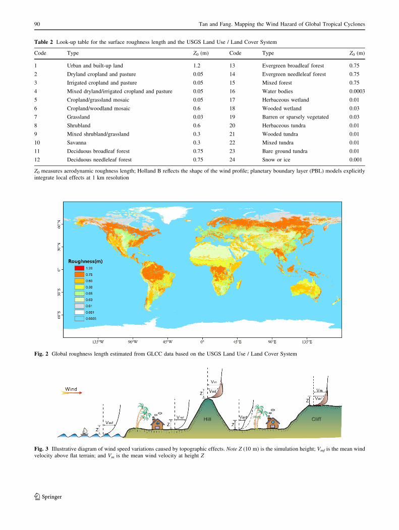
Table 2 Look-up table for the surface roughness length and the USGS Land Use / Land Cover System

Code Type Z0 (m) Code Type Z0 (m)

1 Urban and built-up land 1.2 13 Evergreen broadleaf forest 0.75

2 Dryland cropland and pasture 0.05 14 Evergreen needleleaf forest 0.75

3 Irrigated cropland and pasture 0.05 15 Mixed forest 0.75

4 Mixed dryland/irrigated cropland and pasture 0.05 16 Water bodies 0.0003

5 Cropland/grassland mosaic 0.05 17 Herbaceous wetland 0.01

6 Cropland/woodland mosaic 0.6 18 Wooded wetland 0.03

7 Grassland 0.03 19 Barren or sparsely vegetated 0.03

8 Shrubland 0.6 20 Herbaceous tundra 0.01

9 Mixed shrubland/grassland 0.3 21 Wooded tundra 0.01

10 Savanna 0.3 22 Mixed tundra 0.01

11 Deciduous broadleaf forest 0.75 23 Bare ground tundra 0.01

12 Deciduous needleleaf forest 0.75 24 Snow or ice 0.001

Z0 measures aerodynamic roughness length; Holland B reflects the shape of the wind profile; planetary boundary layer (PBL) models explicitly

integrate local effects at 1 km resolution

Fig. 2 Global roughness length estimated from GLCC data based on the USGS Land Use / Land Cover System

Fig. 3 Illustrative diagram of wind speed variations caused by topographic effects. Note Z (10 m) is the simulation height; Vmf is the mean wind

velocity above flat terrain; and Vm is the mean wind velocity at height Z

123

90 Tan and Fang. Mapping the Wind Hazard of Global Tropical Cyclones

their different degrees of terrain simplification (Maharani

et al. 2009).

After a systematic comparison of the codes of Europe

(BSI 2005), the United States (ASCE 2006), Japan (AIJ

2004), China (CECS 2006), and Australian / New Zealand

(Standards Australia / Standards New Zealand 2002), we

selected the European standard for its detailed speed-up

factor computation method and complete terrain classifi-

cation. According to the standard, terrain features are cat-

egorized into ground, cliff (or escarpment), hill (or ridge),

and valley, and the technical details for deriving the speed-

up factors can be found in Annex A.3 of BSI (2005).

The methods in the building codes were originally

developed for construction design at specific sites where

the terrain type can be easily observed and determined. In

this study, we combine mesoscale wind field modeling with

microscale speed-up modifications by considering topo-

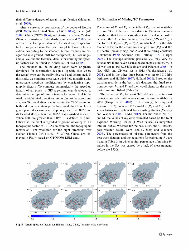
graphic factors. To compute automatically the speed-up

factors of all pixels, a GIS algorithm was developed to

determine the type of terrain feature for every pixel in the

world at eight wind directions. According to the algorithm,

a given TC wind direction is within the 22.5� sector on

both sides of a certain prevailing wind direction. For a

given pixel, if its windward slope is greater than 0.05� andits leeward slope is less than 0.05�, it is classified as a cliff.

When both are greater than 0.05�, it is defined as a hill.

Otherwise, the pixel is regarded as ground or valley with a

topographic factor of 1.0. As an example, the topographic

factors at 1 km resolution for the eight directions over

Hainan Island (108�–111�E, 18�–20�N), China, are dis-

played in Fig. 4 based on GTOPO30 DEM data.

3.3 Estimation of Missing TC Parameters

The values of Pc and Vm, especially of Rm, are not available

in some TCs of the best track datasets. Previous research

has shown that there is a significant statistical relationship

between the TC central pressure difference (DP) and Vm in

the form of Vm = A(Pn - Pc)B, in which DP is the dif-

ference between the environmental pressure (Pn) and the

TC central pressure (Pc), and A and B are fitting constants

(Takahashi 1939; Atkinson and Holliday 1977; Harper

2002). The average ambient pressure, Pn, may vary by

several hPa in the seven basins; based on past studies, Pn in

NI was set to 1013.25 hPa (Islam and Peterson 2008), in

NA, NEP, and CP was set to 1013 hPa (Landsea et al.

2004), and in the other three basins was set to 1010 hPa

(Atkinson and Holliday 1977; Holland 2008). Based on the

existing records in the best track datasets, the fitted rela-

tions between Vm and Pc and their coefficients for the seven

basins are established (Table 3).

The values of Rm for most TCs did not exist in most

historical records until observations became available in

2001 (Knapp et al. 2010). In this study, the empirical

functions of Rm to other TC variables (Pn and lat) in the

seven basins were obtained from existing studies (Vickery

and Wadhera 2008; FEMA 2012). For the NWP, NI, SP,

and SI, the values of Rm were estimated based on the Joint

Typhoon Warning Center (JTWC) dataset as integrated

into IBTrACS. Whereas for the NA, NEP, and CP basins,

past research results were used (Vickery and Wadhera

2008). The percentages of missing parameters from the

best track datasets and the equations for estimating Rm are

listed in Table 3, in which a high percentage of missing Pc

values in the NA was caused by a lack of measurements

before the 1950s.

Fig. 4 Terrain speed-up factors for Hainan Island, China, for eight wind directions

123

Int J Disaster Risk Sci 91

To reflect temporal changes in wind, the simultaneous

wind fields of a TC can be simulated over short temporal

intervals, such as 10 or 15 min. In this study, all parameters

in the best track datasets were linearly interpolated to

10 min (Li et al. 2014). The TCs selected in this work

included all land-falling TCs and all bypassing TCs with a

gradient wind exceeding 5.5 m/s over land (terrain and

roughness effects were not considered); TCs with no

influence on land were excluded from simulation (Table 4).

3.4 Wind Field Validation

Based on the above wind field models, the instantaneous

wind field, which is referred to as a snapshot, at any

specific time can be simulated, and the maximum of all

snapshots can be derived for each TC (called a footprint).

In this study, the footprints of historical TC events

(Table 4) were computed based on the simulated snapshots

at 10-min intervals, including the strongest 3-s gust wind

and both 2- and 10-min sustained winds.

The gradient models used in this study have been widely

validated in NA (Willoughby et al. 2006), NEP (Wil-

loughby et al. 2006), and SP (McConochie et al. 2004), as

well as the PBL model in SP. For NWP, NI, and SI, the

same PBL models were chosen to simulate the wind field

basin as listed in Table 1. Few local, validated studies

based on these models are available in NWP, NI, and SI.

To show the performance of the models used in the

NWP, the modeled winds were compared with ground-

based wind observations in China. The wind observation

data were obtained from ground weather stations. The

modeled and observed time series of 10-min sustained

winds for four strong TCs making landfall in China are

plotted in Fig. 5. To understand the overall accuracy of the

maximum wind time series, the observed and modeled

maximum 10-min sustained winds and 3-s gust winds are

plotted in Fig. 6 based on the observed daily maximum

winds for 36 TCs during the period 1970–2014 from 25

stations located in Hainan Island, China.

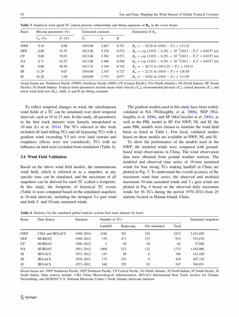
Table 3 Empirical wind speed-TC central pressure relationships and fitting equations of Rm in the seven basins

Basin Missing parameters (%) Estimated constants Estimation of Rm

Vm (%) Pc (%) Pn A B

NWP 9.18 0.00 1010.00 2.607 0.751 Rm = - 18.29 ln (1010 - Pc) ? 113.23

NEP 0.00 51.97 1013.00 5.278 0.574 Rm = exp (3.015 - 6.291 9 10-5(1013 - Pc)2 ? 0.0337 lat)

CP 0.00 70.07 1013.00 5.381 0.571 Rm = exp (3.015 - 6.291 9 10-5(1013 - Pc)2 ? 0.0337 lat)

NA 0.71 63.55 1013.00 5.466 0.566 Rm = exp (3.015 - 6.291 9 10-5(1013 - Pc)2 ? 0.0337 lat)

NI 0.00 68.56 1013.25 2.248 0.742 Rm = - 26.73 ln (1013.25 - Pc) ? 142.41

SP 11.29 0.07 1010.00 2.347 0.727 Rm = - 22.31 ln (1010 - Pc) ? 126.50

SI 16.20 3.20 1010.00 2.753 0.677 Rm = - 18.82 ln (1010 - Pc) ? 111.95

Ocean basins are: Northwest Pacific (NWP); Northeast Pacific (NEP); CP (Central Pacific); NA (North Atlantic); NI (North Indian); SP (South

Pacific); SI (South Indian). Tropical storm parameters include mean wind velocity (Vm), environmental pressure (Pn), central pressure (Pc), and

storm wind field size (Rm), while A and B are fitting constants

Table 4 Statistics for the simulated global tropical cyclone best track datasets by basin

Basin Data Source Duration Number of TCs Simulated snapshots

Landfall Bypassing Not simulated Total

NWP CMA and IBTrACS 1949–2014 1340 701 192 2233 2,101,692

NEP HURDAT 1949–2012 170 471 273 914 551,670

CP HURDAT 1950–2012 3 29 30 62 37,508

NA HURDAT 1851–2012 1068 513 132 1713 1,542,086

NI IBTrACS 1972–2012 147 49 0 196 143,420

SP IBTrACS 1970–2012 175 255 9 439 407,734

SI IBTrACS 1973–2012 160 295 92 547 549,851

Ocean basins are: NWP Northwest Pacific, NEP Northeast Pacific, CP Central Pacific, NA North Atlantic, NI North Indian, SP South Pacific, SI

South Indian. Data sources include: CMA China Meteorological Administration, IBTrACS International Best Track Archive for Climate

Stewardship, and HURDAT U.S. National Hurricane Center’s North Atlantic hurricane database

123

92 Tan and Fang. Mapping the Wind Hazard of Global Tropical Cyclones

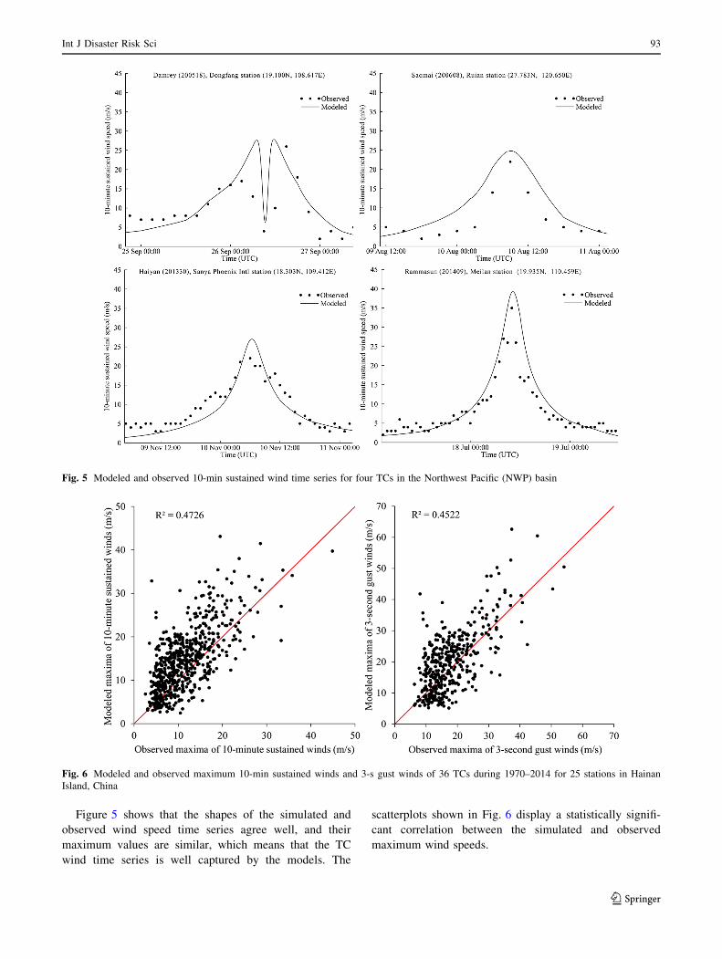
Figure 5 shows that the shapes of the simulated and

observed wind speed time series agree well, and their

maximum values are similar, which means that the TC

wind time series is well captured by the models. The

scatterplots shown in Fig. 6 display a statistically signifi-

cant correlation between the simulated and observed

maximum wind speeds.

Fig. 5 Modeled and observed 10-min sustained wind time series for four TCs in the Northwest Pacific (NWP) basin

Fig. 6 Modeled and observed maximum 10-min sustained winds and 3-s gust winds of 36 TCs during 1970–2014 for 25 stations in Hainan

Island, China

123

Int J Disaster Risk Sci 93

Bias in these parametric models might be introduced

from a range of factors. One of the major reasons that our

wind field modeling may not be realistic is that one of the

key local factors—land use/cover—was kept constant

using global land cover data from year 2000 only, instead

of using data corresponding to each year. In addition, errors

may also be introduced owing to inaccurate or insufficient

resolution of the input data and limited model skill.

3.5 Wind Hazard Analysis

The generalized extreme value (GEV) theory is often

applied to quantify the relationship between the intensity

and frequency of extreme natural events (Goldstein et al.

2008). The Gumbel distribution is usually selected for wind

distribution fitting (Rupp and Lander 1996; An and Pandey

2005; BSI 2005); its cumulative distribution function

(CDF) is

F x; n; hð Þ ¼ exp �exp � x� nð Þ=h½ �f g ð3Þ

where the scale parameter is h and the location parameter is

n. We obtain the moment estimates of h and n as h ¼ffiffiffi6

pS=p and n ¼ �X � ch, and c is Euler’s constant

(0.577216) (Tiago de Oliveira 1963). In this study, �X and

S are the mean and standard deviation of the annual

maximum TC wind speed, which can be derived from the

time series of the simulated historical footprints. The wind

speeds for a T-year return period can be estimated using

VT ¼ n� hln �ln 1� 1=Tð Þ½ � ð4Þ

In addition to the expected wind speeds at specific return

periods, the uncertainty in the estimations is of great

importance for understanding and applying wind hazard

maps. In this study, uncertainty was quantified via a

confidence test. The margin of error at the 95% confidence

interval (CI) of wind speeds for a T-year return period can

be expressed by

VME¼Za=2

ffiffiffiffiffiffiffiffiffiffiffiffiffiffiffiffiffiffiffiffiffiffiffiffiffiffiffiffiffiffiffiffiffiffiffiffiffiffiffiffiffiffiffiffiffiffiffiffiffiffiffiffiffiffiffiffiffiffiffiffiffiffiffiffiffiffiffiffiffiffiffiffiffiffiffiffiffiffiffiffiffiffiffiffiffiffiffiffiffiffiffiffiffiffiffiffiffiffiffiffiffiffiffiffiffiffiffiffiffiffiffiffiffiffiffiffiffiffiffiffiffiffiffiffiffiffiffiffiffiffiffiffiVarðnÞþVarðhÞ ln �ln 1�1=Tð Þ½ �f g2�2 ln �ln 1�1=Tð Þ½ �f gCovðn;hÞ

q

ð5Þ

where 1�a, 0.95 is the significance level, and Za/2 is the

upper a/2 quantile of standard normal distribution

estimated as 1.96. Variances in n and h are expressed by

Var n� �

and Var h� �

estimated as 1:1678h2=n and

1:1h2=n, and the covariance of n and h is Cov n;h� �

estimated as 0:1229h2=n. The relative uncertainty in the

wind hazard estimation can be expressed as

VRE ¼ VME=VT � 100% ð6Þ

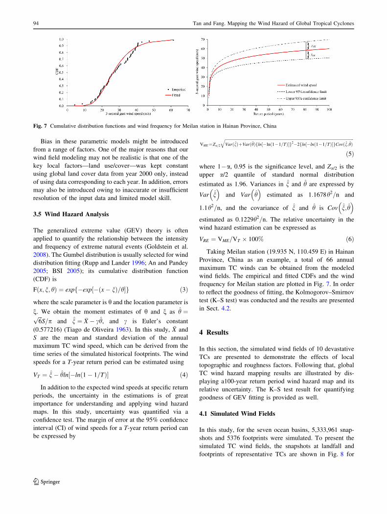
Taking Meilan station (19.935 N, 110.459 E) in Hainan

Province, China as an example, a total of 66 annual

maximum TC winds can be obtained from the modeled

wind fields. The empirical and fitted CDFs and the wind

frequency for Meilan station are plotted in Fig. 7. In order

to reflect the goodness of fitting, the Kolmogorov–Smirnov

test (K–S test) was conducted and the results are presented

in Sect. 4.2.

4 Results

In this section, the simulated wind fields of 10 devastative

TCs are presented to demonstrate the effects of local

topographic and roughness factors. Following that, global

TC wind hazard mapping results are illustrated by dis-

playing a100-year return period wind hazard map and its

relative uncertainty. The K–S test result for quantifying

goodness of GEV fitting is provided as well.

4.1 Simulated Wind Fields

In this study, for the seven ocean basins, 5,333,961 snap-

shots and 5376 footprints were simulated. To present the

simulated TC wind fields, the snapshots at landfall and

footprints of representative TCs are shown in Fig. 8 for

Fig. 7 Cumulative distribution functions and wind frequency for Meilan station in Hainan Province, China

123

94 Tan and Fang. Mapping the Wind Hazard of Global Tropical Cyclones

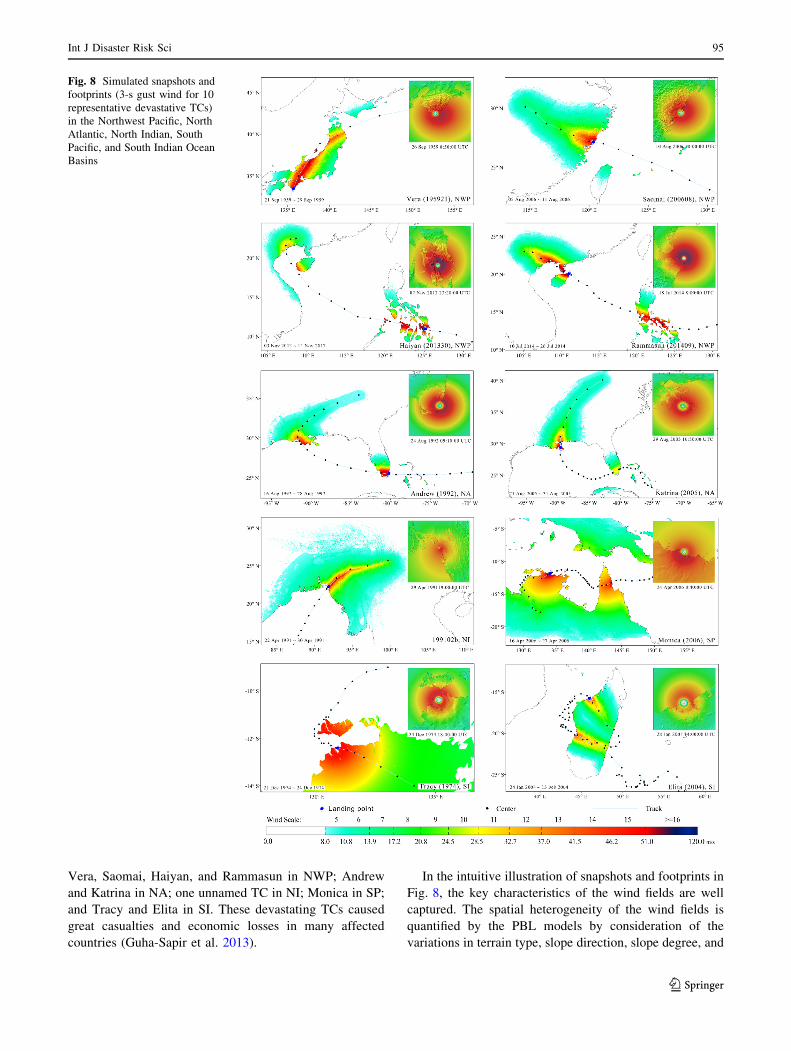
Vera, Saomai, Haiyan, and Rammasun in NWP; Andrew

and Katrina in NA; one unnamed TC in NI; Monica in SP;

and Tracy and Elita in SI. These devastating TCs caused

great casualties and economic losses in many affected

countries (Guha-Sapir et al. 2013).

In the intuitive illustration of snapshots and footprints in

Fig. 8, the key characteristics of the wind fields are well

captured. The spatial heterogeneity of the wind fields is

quantified by the PBL models by consideration of the

variations in terrain type, slope direction, slope degree, and

Fig. 8 Simulated snapshots and

footprints (3-s gust wind for 10

representative devastative TCs)

in the Northwest Pacific, North

Atlantic, North Indian, South

Pacific, and South Indian Ocean

Basins

123

Int J Disaster Risk Sci 95

surface roughness length. Moreover, there is a distinct

difference between the winds over the sea and land, which

is usually caused by the rapid decay of TCs after landfall.

Asymmetry in the simulated instantaneous wind fields are

captured because the gradient models are able to integrate

the effect of TC forwarding.

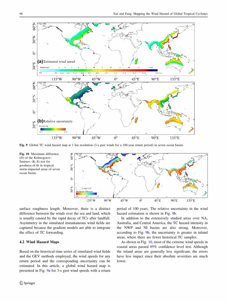
4.2 Wind Hazard Maps

Based on the historical time series of simulated wind fields

and the GEV methods employed, the wind speeds for any

return period and the corresponding uncertainty can be

estimated. In this article, a global wind hazard map is

presented in Fig. 9a for 3-s gust wind speeds with a return

period of 100 years. The relative uncertainty in the wind

hazard estimation is shown in Fig. 9b.

In addition to the extensively studied areas over NA,

Australia, and Central America, the TC hazard intensity in

the NWP and NI basins are also strong. Moreover,

according to Fig. 9b, the uncertainty is greater in inland

areas, where there are fewer historical TC samples.

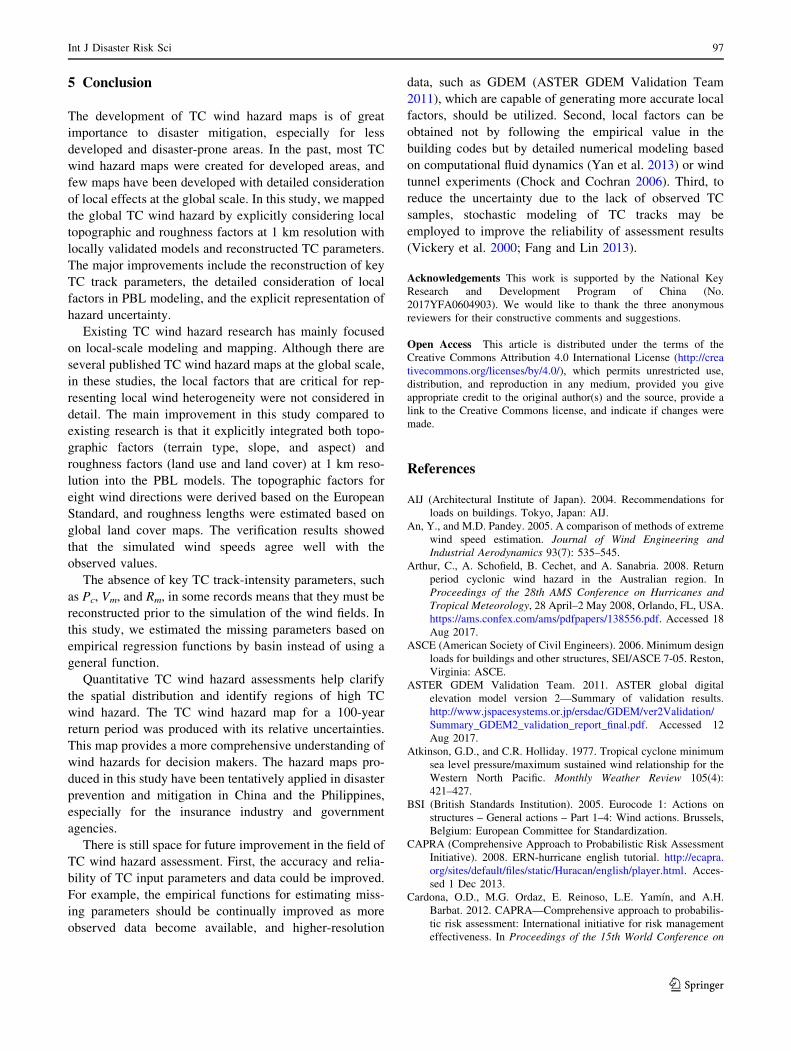
As shown in Fig. 10, most of the extreme wind speeds in

coastal areas passed 95% confidence level test. Although

the inland areas are generally less significant, the errors

have less impact since their absolute severities are much

lower.

Fig. 9 Global TC wind hazard map at 1 km resolution (3-s gust winds for a 100-year return period) in seven ocean basins

Fig. 10 Maximum difference

(D) of the Kolmogorov–

Smirnov (K–S) test for

goodness-of-fit in tropical

storm-impacted areas of seven

ocean basins

123

96 Tan and Fang. Mapping the Wind Hazard of Global Tropical Cyclones

5 Conclusion

The development of TC wind hazard maps is of great

importance to disaster mitigation, especially for less

developed and disaster-prone areas. In the past, most TC

wind hazard maps were created for developed areas, and

few maps have been developed with detailed consideration

of local effects at the global scale. In this study, we mapped

the global TC wind hazard by explicitly considering local

topographic and roughness factors at 1 km resolution with

locally validated models and reconstructed TC parameters.

The major improvements include the reconstruction of key

TC track parameters, the detailed consideration of local

factors in PBL modeling, and the explicit representation of

hazard uncertainty.

Existing TC wind hazard research has mainly focused

on local-scale modeling and mapping. Although there are

several published TC wind hazard maps at the global scale,

in these studies, the local factors that are critical for rep-

resenting local wind heterogeneity were not considered in

detail. The main improvement in this study compared to

existing research is that it explicitly integrated both topo-

graphic factors (terrain type, slope, and aspect) and

roughness factors (land use and land cover) at 1 km reso-

lution into the PBL models. The topographic factors for

eight wind directions were derived based on the European

Standard, and roughness lengths were estimated based on

global land cover maps. The verification results showed

that the simulated wind speeds agree well with the

observed values.

The absence of key TC track-intensity parameters, such

as Pc, Vm, and Rm, in some records means that they must be

reconstructed prior to the simulation of the wind fields. In

this study, we estimated the missing parameters based on

empirical regression functions by basin instead of using a

general function.

Quantitative TC wind hazard assessments help clarify

the spatial distribution and identify regions of high TC

wind hazard. The TC wind hazard map for a 100-year

return period was produced with its relative uncertainties.

This map provides a more comprehensive understanding of

wind hazards for decision makers. The hazard maps pro-

duced in this study have been tentatively applied in disaster

prevention and mitigation in China and the Philippines,

especially for the insurance industry and government

agencies.

There is still space for future improvement in the field of

TC wind hazard assessment. First, the accuracy and relia-

bility of TC input parameters and data could be improved.

For example, the empirical functions for estimating miss-

ing parameters should be continually improved as more

observed data become available, and higher-resolution

data, such as GDEM (ASTER GDEM Validation Team

2011), which are capable of generating more accurate local

factors, should be utilized. Second, local factors can be

obtained not by following the empirical value in the

building codes but by detailed numerical modeling based

on computational fluid dynamics (Yan et al. 2013) or wind

tunnel experiments (Chock and Cochran 2006). Third, to

reduce the uncertainty due to the lack of observed TC

samples, stochastic modeling of TC tracks may be

employed to improve the reliability of assessment results

(Vickery et al. 2000; Fang and Lin 2013).

Acknowledgements This work is supported by the National Key

Research and Development Program of China (No.

2017YFA0604903). We would like to thank the three anonymous

reviewers for their constructive comments and suggestions.

Open Access This article is distributed under the terms of the

Creative Commons Attribution 4.0 International License (http://crea

tivecommons.org/licenses/by/4.0/), which permits unrestricted use,

distribution, and reproduction in any medium, provided you give

appropriate credit to the original author(s) and the source, provide a

link to the Creative Commons license, and indicate if changes were

made.

References

AIJ (Architectural Institute of Japan). 2004. Recommendations for

loads on buildings. Tokyo, Japan: AIJ.

An, Y., and M.D. Pandey. 2005. A comparison of methods of extreme

wind speed estimation. Journal of Wind Engineering and

Industrial Aerodynamics 93(7): 535–545.

Arthur, C., A. Schofield, B. Cechet, and A. Sanabria. 2008. Return

period cyclonic wind hazard in the Australian region. In

Proceedings of the 28th AMS Conference on Hurricanes and

Tropical Meteorology, 28 April–2 May 2008, Orlando, FL, USA.

https://ams.confex.com/ams/pdfpapers/138556.pdf. Accessed 18

Aug 2017.

ASCE (American Society of Civil Engineers). 2006. Minimum design

loads for buildings and other structures, SEI/ASCE 7-05. Reston,

Virginia: ASCE.

ASTER GDEM Validation Team. 2011. ASTER global digital

elevation model version 2—Summary of validation results.

http://www.jspacesystems.or.jp/ersdac/GDEM/ver2Validation/

Summary_GDEM2_validation_report_final.pdf. Accessed 12

Aug 2017.

Atkinson, G.D., and C.R. Holliday. 1977. Tropical cyclone minimum

sea level pressure/maximum sustained wind relationship for the

Western North Pacific. Monthly Weather Review 105(4):

421–427.

BSI (British Standards Institution). 2005. Eurocode 1: Actions on

structures – General actions – Part 1–4: Wind actions. Brussels,

Belgium: European Committee for Standardization.

CAPRA (Comprehensive Approach to Probabilistic Risk Assessment

Initiative). 2008. ERN-hurricane english tutorial. http://ecapra.

org/sites/default/files/static/Huracan/english/player.html. Acces-

sed 1 Dec 2013.

Cardona, O.D., M.G. Ordaz, E. Reinoso, L.E. Yamın, and A.H.

Barbat. 2012. CAPRA—Comprehensive approach to probabilis-

tic risk assessment: International initiative for risk management

effectiveness. In Proceedings of the 15th World Conference on

123

Int J Disaster Risk Sci 97

Earthquake Engineering, 24–28 September 2012, Lisbon, Por-

tugal. http://www.iitk.ac.in/nicee/wcee/article/WCEE2012_

0726.pdf. Accessed 18 Aug 2017.

CECS (China Association for Engineering Construction Standardiza-

tion). 2006. Load code for design of building structures

GB50009-2001. Beijing: China Architecture and Building Press

(in Chinese).

Chen, K. 1994. A computation method for typhoon wind field.

Tropical Oceanology 13(2): 41–48 (in Chinese).

Chock, G.Y.K., and L. Cochran. 2006. Erratum to ‘‘Modeling of

topographic wind speed effects in Hawaii’’: [Journal of Wind

Engineering & Industrial Aerodynamics: Volume 93, issue 8,

August 2005, pp. 623–638]. Journal of Wind Engineering and

Industrial Aerodynamics 94(3): 173–187.

CIMNE (International Centre for Numerical Methods in Engineer-

ing). 2013. Probabilistic modeling of natural risks at the global

level: Global risk model. Geneva: UNISDR.

Davenport, A.G., P.N. Georgiou, and D. Surry. 1985. A hurricane

wind risk study for the Eastern Caribbean, Jamaica and Belize,

with special consideration to the influence of topography.

London and Ontario, Canada: Boundary Layer Wind Tunnel

Laboratory and Faculty of Engineering Science, University of

Western Ontario.

Davenport, A.G., C.S.B. Grimmond, T.R. Oke, and J. Wieringa. 2000.

Estimating the roughness of cities and sheltered country. In

Proceedings of the 12th Conference on Applied Climatology,

8–11 May 2000, American Meteorological Society, Asheville,

North Carolin, USA, 96–99.

Elsner, J.B., T.H. Jagger, and K.-B. Liu. 2008. Comparison of

hurricane return levels using historical and geological records.

Journal of Applied Meteorology and Climatology 47(2):

368–374.

Emanuel, K., S. Ravela, E. Vivant, and C. Risi. 2006. A statistical

deterministic approach to hurricane risk assessment. Bulletin of

the American Meteorological Society 87(3): 299–314.

ESDU (Engineering Sciences Data Unit). 1983. Strong winds in the

atmospheric boundary layer. Part 2: Discrete gust speeds, ESU–

83045. London: ESDU.

Fang, W., and W. Lin. 2013. A review on typhoon wind field

modeling for disaster risk assessment. Progress in Geography

32(6): 852–867 (in Chinese).

FEMA (Federal Emergency Management Agency). 2012. Hazus—

MH 2.1 Hurricane model technical manual. Washington, DC:

Mitigation Division, Department of Homeland Security Federal

Emergency Management Agency.

FIU (Florida International University). 2011. Florida public hurricane

loss model 4.1. Miami, FL: Florida International University.

Georgiou, P.N., A.G. Davenport, and B.J. Vickery. 1983. Design

wind speeds in regions dominated by tropical cyclones. Journal

of Wind Engineering and Industrial Aerodynamics 13(1–3):

139–152.

Giuliani, G., and P. Peduzzi. 2011. The PREVIEW Global Risk Data

Platform: A geoportal to serve and share global data on risk to

natural hazards. Natural Hazards and Earth System Science

11(1): 53–66.

Goldstein, J., J.-D. Langlois, M. Dimitrijevic, M. Sadoud, and V.

David. 2008. Approaches for extreme wind speed assessment: A

case study. In Proceedings of the 7th World Wind Energy

Conference, 24–26 June 2008, Helimax Energy Inc., Kingston,

Canada, 1–8.

Guha-Sapir, D., R. Below, and P. Hoyois. 2013. EM-DAT: Interna-

tional disaster database. Brussels, Belgium: Universite Catholi-

que de Louvain. http://www.emdat.be. Accessed 1 Sept 2017.

Harper, B.A. 2001. Queensland climate change and community

vulnerability to tropical cyclones: Ocean hazards assessment –

Stage 1. Queensland: Systems Engineering Australia Pty Ltd,

Bureau of Meteorology, and James Cook University.

Harper, B.A. 2002. Tropical cyclone parameter estimation in the

Australian region: Wind–pressure relationships and related

issues for engineering planning and design—A discussion paper.

SEA Report No. J0106-PR003E. Report prepared by Systems

Engineering Australia Pty. Report prepared for Woodside

Energy.

Harper, B.A., and G.J. Holland. 1999. An updated parametric model

of the tropical cyclone. In Proceedings of the 23rd Conference

on Hurricanes and Tropical Meteorology, 10–15 January 1999,

American Meteorological Society, Dallas, Texas, USA.

Holland, G. 2008. A revised hurricane pressure-wind model. Monthly

Weather Review 136(9): 3432–3445.

Huang, Z., D.V. Rosowsky, and P.R. Sparks. 2001. Long-term

hurricane risk assessment and expected damage to residential

structures. Reliability Engineering and System Safety 74(3):

239–249.

Islam, T., and R.E. Peterson. 2008. Tropical cyclone wind charac-teristics for the Bangladesh coast using Monte Carlo simulation.

Journal of Applied Sciences 8(7): 1249–1255.

Jakobsen, F., and H. Madsen. 2004. Comparison and further

development of parametric tropical cyclone models for storm

surge modelling. Journal of Wind Engineering and Industrial

Aerodynamics 92(5): 375–391.

Jarvis, A., H.I. Reuter, A. Nelson, and E. Guevara. 2008. Hole-filled

SRTM for the globe version 4. Available from the CGIAR-CSI

SRTM 90 m Database. http://srtm.csi.cgiar.org. Accessed 23 Jul

2017.

Knapp, K.R., M.C. Kruk, D.H. Levinson, H.J. Diamond, and C.J.

Neumann. 2010. The international best track archive for climate

stewardship (IBTrACS): Unifying tropical cyclone data. Bulletin

of the American Meteorological Society 91(3): 363–376.

Landsea, C.W., C. Anderson, N. Charles, G. Clark, J. Dunion, J.

Fernandez-Partagas, P. Hungerford, C. Neumann, and M.

Zimmer. 2004. The Atlantic hurricane database re-analysis

project: Documentation for the 1851–1910 alterations and

additions to the HURDAT database. In Hurricanes and

typhoons: Past, present and future, ed. R.J. Murnane, and K.B.

Liu, 177–221. New York: Columbia University Press.

Landsea, C.W., and J.L. Franklin. 2013. Atlantic hurricane database

uncertainty and presentation of a new database format. Monthly

Weather Review 141(10): 3576–3592.

Lee, Y.-K., S. Lee, and H.-S. Kim. 2009. Evaluation of wind hazard

over Jeju Island. In Proceedings of the 7th Asia-Pacific

Conference on Wind Engineering, 8–12 November 2009, Taipei,

China. http://www.iawe.org/Proceedings/7APCWE/M2B_6.pdf.

Accessed 25 Jul 2017.

Levinson, D.H., H.J. Diamond, K.R. Knapp, M.C. Kruk, and E.J.

Gibney. 2010. Toward a homogenous global tropical cyclone

best-track dataset. Bulletin of the American Meteorological

Society 91(3): 377–380.

Li, X.Y., W.H. Fang, and W. Lin. 2014. Comparison of interpolation

methods for tropical cyclone track and intensity over North-

western Pacific basin. Journal of Beijing Normal University

(Natural Science) 50(2): 111–116 (in Chinese).

Lin, W., and W.H. Fang. 2013. Regional characteristics of Holland B

parameter in typhoon wind field model for Northwest Pacific.

Tropical Geography 33(2): 124–132 (in Chinese).

Loveland, T.R., B.C. Reed, J.F. Brown, D.O. Ohlen, Z. Zhu, L. Yang,

and J.W. Merchant. 2000. Development of a global land cover

characteristics database and IGBP DISCover from 1 km

AVHRR data. International Journal of Remote Sensing

21(6–7): 1303–1330.

Maharani, Y.N., S. Lee, and Y.-K. Lee. 2009. Topographical effects

on wind speed over various terrains: A case study for Korean

123

98 Tan and Fang. Mapping the Wind Hazard of Global Tropical Cyclones

Peninsula. In Proceedings of the 7th Asia-Pacific Conference on

Wind Engineering, 8–12 November 2009, Taipei, China. http://

www.iawe.org/Proceedings/7APCWE/T2D_5.pdf. Accessed 25

Jul 2017.

McConochie, J.D., T.A. Hardy, and L.B. Mason. 2004. Modelling

tropical cyclone over-water wind and pressure fields. Ocean

Engineering 31(14): 1757–1782.

Mctaggart-Cowan, R., L.F. Bosart, C.A. Davis, E.H. Atallah, J.R.

Gyakum, and K.A. Emanuel. 2006. Analysis of Hurricane

Catarina (2004). Monthly Weather Review 134(11): 3029–3053.

Meng, Y., M. Matsui, and K. Hibi. 1997. A numerical study of the

wind field in a typhoon boundary layer. Journal of Wind

Engineering and Industrial Aerodynamics 67–68: 437–448.

Ngo, T.T., and C.W. Letchford. 2009. Experimental study of

topographic effects on gust wind speed. Journal of Wind

Engineering and Industrial Aerodynamics 97(9–10): 426–438.

Nolan, D.S., J.A. Zhang, and D.P. Stern. 2009. Evaluation of

planetary boundary layer parameterizations in tropical cyclones

by comparison of in situ observations and high-resolution

simulations of Hurricane Isabel (2003). Part I: Initialization,

maximum winds, and the outer-core boundary layer. Monthly

Weather Review 137(11): 3651–3674.

Prigent, C., I. Tegen, F. Aires, B. Marticorena, and M. Zribi. 2005.

Estimation of the aerodynamic roughness length in arid and

semiarid regions over the globe with the ERS scatterometer.

Journal of Geophysical Research: Atmospheres 110(D9): 1–12.

Ramli, N.I., M.I. Ali, M.S.H. Saad, and T.A. Majid. 2009. Estimation

of the roughness length (zo) in Malaysia using satellite image. In

Proceedings of 7th Asia-Pacific Conference on Wind Engineer-

ing, 8–12 November 2009, Taipei, China. http://www.iawe.org/

Proceedings/7APCWE/T2D_1.pdf. Accessed 23 Jul 2017.

Rupp, J.A., and M.A. Lander. 1996. A technique for estimating

recurrence intervals of tropical cyclone-related high winds in the

tropics: Results for Guam. Journal of Applied Meteorology

35(5): 627–637.

Russell, L.R. 1969. Probability distributions for Texas Gulf coast

hurricane effects of engineering interest. Ph.D. dissertation.

Department of Civil Engineering, Stanford University, Stanford,

California.

SAC (Standardization Administration of China). 2006. Grade of

tropical cyclone GB/T 19201-2006. Beijing: SAC (in Chinese).

Shi, P., and R. Kasperson. 2015. World atlas of natural disaster risk.

London and Beijing: Springer and Beijing Normal University.

Silva, J., C. Ribeiro, and R. Guedes. 2007. Roughness length

classification of Corine Land Cover classes. In Proceedings of

the European Wind Energy Conference, 7–10 May 2007, Milan,

Italy, 1–10.

Skamarock, W.C., J.B. Klemp, J. Dudhia, D.O. Gill, D.M. Barker, W.

Wang, and J.G. Powers. 2005. A description of the advanced

research WRF version 2. Boulder, CO: Mesoscale and Micro-

scale Meteorology Division, National Center for Atmospheric

Research.

Standards Australlia / Standards New Zealand. 2002. Structural

design actions. Part 2: Wind actions AS/NZS 1170.2: 2002.

Sydney and Wellington: Standards Australlia International and

Standards New Zealand.

Summons, N., and C. Arthur. 2011. Tropical cyclone risk model user

guide. Canberra, Australia: Commonwealth of Australia (Geo-

science Australia). https://storage.googleapis.com/google-code-

archive-downloads/v2/code.google.com/tcrm/tcrm_user_guide.

pdf. Accessed 28 Jul 2017.

Takahashi, K. 1939. Distribution of pressure and wind in a typhoon.

Journal of the Meteorological Society of Japan 17(2): 417–421.

Tiago de Oliveira, J. 1963. Decision results for the parameters of the

extreme value (Gumbel) distribution based on the mean and the

standard deviation. Trabajos de Estadistica Y de Investigacion

Operativa 14(1): 61–81.

UNISDR (United Nations International Strategy for Disaster Reduc-

tion). 2009. Global assessment report on disaster risk reduction.

Geneva: United Nations.

UNISDR (United Nations International Strategy for Disaster Reduc-

tion). 2011. Global assessment report on disaster risk reduction.

Geneva: United Nations.

UNISDR (United Nations International Strategy for Disaster Reduc-

tion). 2013. Global assessment report on disaster risk reduction.

Geneva: United Nations.

UNISDR (United Nations International Strategy for Disaster Reduc-

tion). 2015. Global Assessment Report on disaster Risk Reduc-

tion. Geneva: United Nations.

USGS (U.S. Geological Survey). 1996. GTOPO30: Global 30 arc-

seconds digital elevation model. Data available from the U.S.

Geological Survey. https://lta.cr.usgs.gov/GTOPO30. Accessed

21 Jul 2017.

USGS (U.S. Geological Survey). 2001. Global land cover character-

istics database version 2.0. Data available from the U.S.

Geological Survey. https://lta.cr.usgs.gov/GLCC. Accessed 21

Jul 2017.

Vickery, P.J., P.F. Skerlj, and L.A. Twisdale. 2000. Simulation of

hurricane risk in the US using empirical track model. Journal of

Structural Engineering 126(10): 1222–1237.

Vickery, P.J., and D. Wadhera. 2008. Statistical models of Holland

pressure profile parameter and radius to maximum winds of

hurricanes from flight-level pressure and H* Wind data. Journal

of Applied Meteorology and Climatology 47(10): 2497–2517.

Wieringa, J. 1992. Updating the Davenport roughness classification.

Journal of Wind Engineering and Industrial Aerodynamics

41(1): 357–368.

Wieringa, J., A.G. Davenport, C.S.B. Grimmond, and T.R. Oke. 2001.

New revision of Davenport roughness classification. In Pro-

ceedings of the 3rd European and African Conference on Wind

Engineering, 2–6 July 2001, Eindhoven, The Netherlands, 1–8.

Willoughby, H.E., R.W.R. Darling, and M.E. Rahn. 2006. Parametric

representation of the primary hurricane vortex. Part II: A new

family of sectionally continuous profiles. Monthly Weather

Review 134(4): 1102–1120.

Wong, M.L.M., and J.C.L. Chan. 2007. Modeling the effects of land-

sea roughness contrast on tropical cyclone winds. Journal of the

Atmospheric Sciences 64(9): 3249–3264.

Yan, B.W., Q.S. Li, Y.C. He, and P.W. Chan. 2013. Numerical

simulation of topographic effects on wind flow fields over

complex terrain. In Proceedings of the 8th Asia-Pacific Confer-

ence on Wind Engineering, 10–14 December 2013, Chennai,

India, 541–550. Singapore: Research Publishing. http://iawe.org/

Proceedings/8APCWE/B.W.%20Yan.pdf. Accessed 12 Mar

2017.

Ying, M., W. Zhang, H. Yu, X. Lu, J. Feng, Y. Fan, Y. Zhu, and D.

Chen. 2014. An overview of the China Meteorological Admin-

istration tropical cyclone database. Journal of Atmospheric and

Oceanic Technology 31(2): 287–301.

123

Int J Disaster Risk Sci 99