Embed Size (px)
Citation preview

Mapping the Stocks in MICEX:
Who Is Central in Moscow Stock Exchange?
by M. Hakan Eratalay and Evgenii V. Vladimirov
2017/01
Working Paper SeriesDepartment of Economics
European University at St. Petersburg

Eratalay M. H., Vladimirov E. V. (2017) Mapping the stocks in MICEX:
Who is central in Moscow Stock Exchange? European University at St.Petersburg, Department of Economics, Working Paper 2017/01, 40 p.
Abstract: In this article we use partial correlations to derive bidirectional con-nections between the major firms listed in MICEX. We obtain the coefficientsof partial correlation from the correlation estimates of constant conditionalcorrelation GARCH (CCC-GARCH) and consistent dynamic conditionalcorrelation GARCH (cDCC-GARCH) models. We map the graph of partialcorrelations using the Gaussian graphical model and apply network analysis toidentify the most central firms in terms of shock propagation and in terms ofconnectedness with others. Moreover, we analyze some macro characteristicsof the network over time and measure the system vulnerability to externalshocks. Our findings suggest that during the crisis interconnectedness betweenfirms strengthen and system becomes more vulnerable to systemic shocks. Inaddition, we found that the most connected firms are Sberbank and Lukoilwhile most central in terms of systemic risk are Gazprom and FGC UES.
Keywords: Multivariate GARCH, Volatility Spillovers, Network connections,MICEX
JEL classification: C01, C13, C32, C52
M. Hakan Eratalay, Named Professor of Financial Econometrics in theDepartment of Economics at the European University at St. Petersburg,3 Gagarinskaya Street, St. Petersburg, 191187, Russia.
[email protected] V. Vladimirov, European University at St. Petersburg,3 Gagarinskaya Street, St. Petersburg, 191187, Russia.
c� M. H. Eratalay, E. Vladimirov, 2017

Mapping the stocks in MICEX:
Who is central in Moscow Stock Exchange?
M. Hakan Eratalay! Evgenii V. Vladimirovy
February 2, 2017
Preliminary version
Abstract
In this article we use partial correlations to derive bidirectional connections between
major Örms listed in MICEX. We obtain coe¢cients of partial correlation from the
correlation estimates of constant conditional correlation GARCH (CCC-GARCH) and
consistent dynamic conditional correlation GARCH (cDCC-GARCH) models. We map
the graph of partial correlations using the Gaussian graphical model and apply network
analysis to identify the most central Örms in terms of shock propagation and in terms
of connectedness with others. Moreover, we analyze some macro characteristics of
the network over time and measure the system vulnerability to external shocks. Our
Öndings suggest that during the crisis interconnectedness between Örms strengthens
and the system becomes more vulnerable to systemic shocks. In addition, we found
that the most connected Örms are Sberbank and Lukoil, while most central in terms
of systemic risk are Gazprom and FGC UES.
JEL: C01, C13, C32, C52Keywords: Multivariate GARCH, Volatility Spillovers, Network connections, MICEX
1 Introduction
The Önancial crisis of 2008 exposed the needs for better understanding of risks in Önancial
market and in economy in general. SpeciÖcally, systemic risk became one of the most im-
portant issues and encouraged a lot of literature in Önance mainly after the crisis of 2008.
!Corresponding author. Named Professor of Financial Econometrics in the Department of Economics
at the European University at St. Petersburg. Professorship position Önanced by the MDM Bank. Email:
[email protected] student. European University at Saint Petersburg, Department of Economics
1

There are several approaches to measure systemic risk such as SRISK measure proposed by
Brownless and Engle (2016) or CoVaR method by Adrian and Brunnermeier (2016) among
many others.
Linkages between Örms is one of the key channels of how systemic risk spreads throughout
the system. Once a Örm experiences a negative extrenalities it becomes dangerous not
only for the Örm and its bondolders, as the capitalizations of the Örm fall, but also might
negatively a§ect the whole economy through the trading or loan channels. Hence, estimation
of these connections play a central role in understanding behaviour of such systemic risk.
A widely used approach to describe the connectedness among the number of companies is
the usage of graphs as a network theory application. There is a number of papers, which
describe Önancial and economic data from the network theory perspective. For example,
interbank connections in the paper of Brownless, Hans, Nualart (2014), interconnectedness
among Önancial institutions (Diebold, Yilmaz (2014)) and among the major corporation in
U.S.(Bariggozi, Brownless (2016)) and Australia (Anufriev and Panchenko (2015)).
Moreover, network theory helps us not only to visualize graph of connectedness but also
to make some conclusions based on appropriate measures of network theory. In our paper
we identify top connected Örms and top systemic contributors in static model and over time
in Russian Stock Market. In addition, we calculate vulnerability of the system as an average
of the quantitative measures of the possible fall of the system caused by a negative shock to
each Örm. This magnitude can be used as a measure of overall systemic risk in the entire
economy, as it shows sensitivity of the system to negative externalities in general.
In order to construct a network of connectedness we use the Gaussian Graphical Model
(GGM) approach, which is quite new for Önance, while it is widely used in biometrics (see for
example Krumsiek et al. (2011), Rice et al. (2005)). The idea of GGM is to capture linear
bidirectional dependence between two variables measured with partial correlation conditional
on other elements in the system. Separated linear dependence between a pair of Örms showing
partial correlation can be used as a channel through which a shock can be transmitted
from one Örm to another. GGM allows reconstructing graphs of interconnectedness between
components of multivariate random variable, where nodes of the graph represent elements of
this multivariate vector and edges show their conditional dependence. This type of network
of partial correlations between Örms shows not only how well or not the whole economy is
connected, but also how the shocks propagate therein, if some company su§ers from negative
exogenous e§ects.
Firms can be connected in di§erent ways. For example, they can be connected directly
via trading relationships. However, to study interconnectedness in Önancial market we need
more frequent data, than, for instance, companiesí balance sheets. One of the convenient
ways to identify connectedness between Örms is to consider co-movements of their stock
2
returns (see Diebold, Yilmaz (2014)). The idea of this approach is that almost all Örms,
especially the largest ones, spend a lot of resources in order to manage their businesses in
accordance with concurrent market conditions, and virtually all their decisions a§ect their
stock prices. That is why connectedness between stock returns can be taken as a proxy to
the true unobservable connections between Örms. Moreover, such frequent data allows us to
calculate daily measure of systemic risk, which is a considerable advantage for policymakers.
General approach for Önancial data is to take into account volatility connectedness (see
Diebold, Yilmaz (2014)). Volatility often represents fear of investors, hence volatility con-
nectedness is a kind of fear connectedness between investors. For example, in situations of
uncertainty, such as Önancial crises, investors fear more and volatility increases. In a situa-
tion where two Örms are connected, increasing volatility in one Örmís stock returns will lead
to volatility rise of the second one, that is why we should capture volatility connectedness
between two Örms.
In this paper, we bring together the ideas from the papers by Anufriev and Panchenko
(2015), Barigozzi and Brownlees (2016) and Diebold and Yilmaz (2014). One novelty of our
work is in the econometric methodology. We use a VAR model and Kalman Ölter to elimi-
nate unobservable common factor. According to Barigozzi and Brownlees (2016), common
factors, which a§ect the returns, if not Öltered out, will lead to spuriously high correlations
and a fully connected network. Moreover, we compute partial correlations from the condi-
tional correlation estimates obtained from the Constant Conditional Correlation GARCH
model of Bollerslev (1990) and consistent Dynamic Conditional Correlation GARCH model
of Aielli (2008). The former model gives an idea on how the Örms are connected throughout
the data period, while the latter model allows us to pinpoint the connections on a certain
date. Therefore we can comment on how the network connections restructure in reaction to
ináuential changes. Finally, we use the composite likelihood method of Engle et al. (2008)
for estimation. This method successfully avoids the trap of attenuation biases observed in
cDCC-GARCH model.1
To the best of our knowledge, this is the Örst work examining major Örms in the Russian
Stock Market. Our data spans over four years of observations and covers in particular the
year of 2014, when Russia faced a number of problems.
The paper is structured as follows. Section 2 introduces network construction based on
Gaussian graphical model. Section 3 discusses the crucial measures of network analysis.
In Section 4 we introduce the data we use and in the following Section 5 we discuss the
1When the number of series in consideration is large, quasi-maximum likelihood estimators of a cDCC-
GARCH model with variance targeting yields downward biases in the correlation coe¢cient estimates, hence
implying very little variation in the correlations between returns over time. See Engle et al. (2008) for
details.
3

econometric models. Section 6 describes estimation procedure of the econometric models.
Section 7 shows empirical application for Russian Stock Market. Finally, Section 8 details
further discussion. Section 9 concludes the paper.
2 Network construction
Letís consider a graph G = (V;E) with a set of vertices V = f1; :::; ng and a set of edgesE = V %V . If nodes i and j are connected then pair (i; j) 2 E. Based on the type of edges,a graph can be directed or undirected as well as weighted or unweighted. In our work we
focus on undirected weighted graphs meaning that if pair (i; j) 2 E; then (j; i) 2 E, andeach edge has a non-zero weight wi;j that shows the strength of connectedness between nodes
i and j.
To construct a network we use the concept of Gaussian graphical models based on the
work of Buhlmann and Van De Geer (2011), Hastie et al. (2009) and Anufriev and Panchenko
(2015). A Gaussian Graphical Model (GGM) helps to construct a conditional independent
weighted graph G = (V;E) with the Markov property that if nodes i and j are conditionally
independent then (i; j) =2 E. The vertices of the graph correspond to each component ofmultivariate random variable X = fX1; :::; Xng.According to GGM, the coe¢cient of partial correlation can be used to measure the
conditional dependence between any two nodes. Partial correlation between nodes i and j,
i.e. between components Xi and Xj of multivariate variable X, ,i;jj:, measures their linear
dependence excluding the ináuence of the rest of the components of variable X. The idea is
that while ordinary correlation can show high connection between two variables generated
by dependence of these both variables on a third one, the partial correlation measure their
connection eliminating the ináuence of the third variable from both of them. Thus, two
nodes are connected (i; j) 2 E, if and only if they are not conditionally independent, i.e.,i;jj: 6= 0. Moreover, partial correlation between any pairs of nodes is used in GGM as a
weight of an edge in the graph corresponding to that pair, i.e. wi;j = ,i;jj: is the weight of
the edge between nodes i and j.
Before considering how partial correlation can be obtained, let us recall that coe¢cient
of correlation between components Xi and Xj, ri;j, is the coe¢cient of covariance between
them divided by standard deviation of each component, i.e.
ri;j =.i;j.i.j
; (1)
where .i;j is the covariance between Xi and Xj, and .i =p.i;i is the standard deviation
of variable Xi. In other words, correlation between any two components can be expressed
4
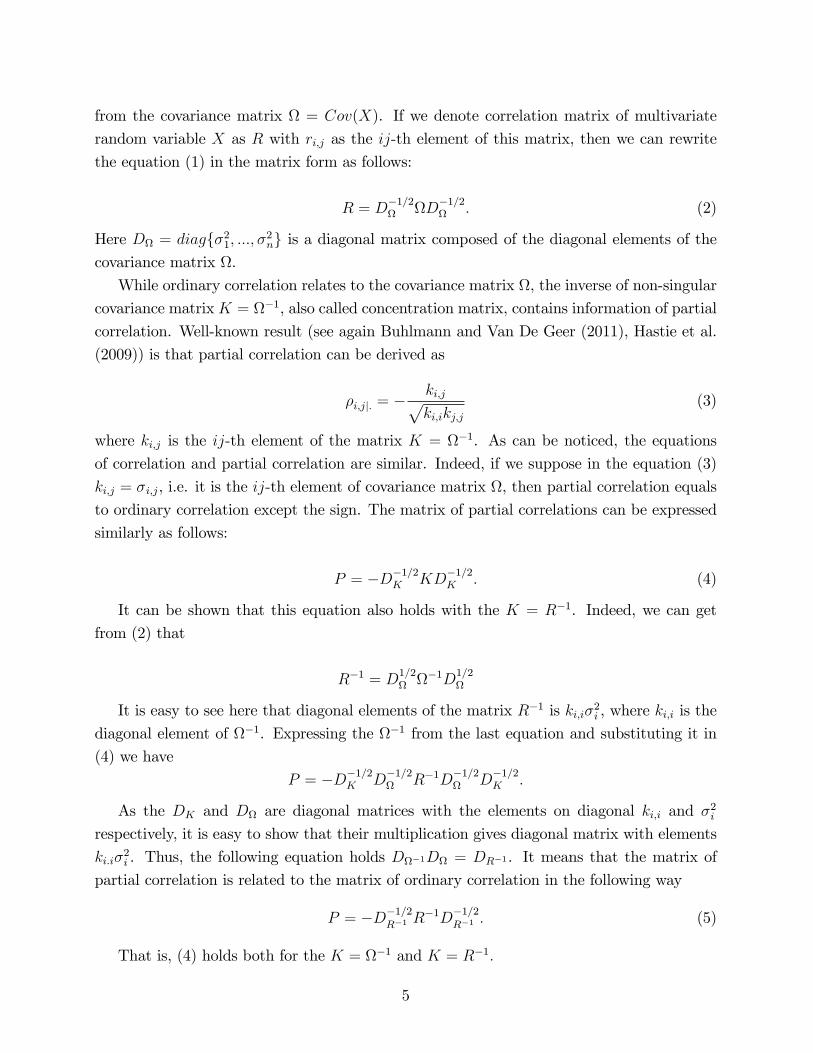
from the covariance matrix & = Cov(X). If we denote correlation matrix of multivariate
random variable X as R with ri;j as the ij-th element of this matrix, then we can rewrite
the equation (1) in the matrix form as follows:
R = D"1=2# &D
"1=2# : (2)
Here D# = diagf.21; :::; .2ng is a diagonal matrix composed of the diagonal elements of thecovariance matrix &.
While ordinary correlation relates to the covariance matrix &, the inverse of non-singular
covariance matrixK = &"1, also called concentration matrix, contains information of partial
correlation. Well-known result (see again Buhlmann and Van De Geer (2011), Hastie et al.
(2009)) is that partial correlation can be derived as
,i;jj: = )ki;jpki;ikj;j
(3)
where ki;j is the ij-th element of the matrix K = &"1. As can be noticed, the equations
of correlation and partial correlation are similar. Indeed, if we suppose in the equation (3)
ki;j = .i;j, i.e. it is the ij-th element of covariance matrix &, then partial correlation equals
to ordinary correlation except the sign. The matrix of partial correlations can be expressed
similarly as follows:
P = )D"1=2K KD
"1=2K : (4)
It can be shown that this equation also holds with the K = R"1. Indeed, we can get
from (2) that
R"1 = D1=2# &"1D
1=2#
It is easy to see here that diagonal elements of the matrix R"1 is ki;i.2i , where ki;i is the
diagonal element of &"1. Expressing the &"1 from the last equation and substituting it in
(4) we have
P = )D"1=2K D
"1=2# R"1D
"1=2# D
"1=2K :
As the DK and D# are diagonal matrices with the elements on diagonal ki;i and .2i
respectively, it is easy to show that their multiplication gives diagonal matrix with elements
ki:i.2i . Thus, the following equation holds D#!1D# = DR!1. It means that the matrix of
partial correlation is related to the matrix of ordinary correlation in the following way
P = )D"1=2R!1 R
"1D"1=2R!1 : (5)
That is, (4) holds both for the K = &"1 and K = R"1:
5

The other common way to represent a graph is adjacency matrix (see Jackson (2008)).
Adjacency matrix A is a matrix of size n % n with a non-zero ij-th element if the nodesi and j are connected and with the zeros otherwise. For an undirected weighted graph the
adjacency matrix is symmetric with entries given by weights of the appropriate nodes. In
the case of GGM the adjacency matrix contains coe¢cient of partial correlation ,i;jj: as the
ij-th element for i 6= j and zeros on the diagonal. Notice that diagonal elements of matrixof partial correlations are minus units given that equation (3) holds. That is, in the matrix
form we have:
A = I + P = I )D"1=2K KD
"1=2K (6)
where I is the identity matrix of size n andK can be both inverse ordinary correlation matrix
R"1 and inverse covariance matrix &"1 of multivariate vector X. Adjacency matrix gives us
not only a method to set up a graph but an opportunity to analyze the graph using tools of
linear algebra. We dwell our attention on such analysis in the next section.
Finally it is important to note the sign of the entries of adjacency matrix constructed on
the base of partial correlation. In network theory weights of edges are usually assumed to
be positive. However, as value of partial correlation spans between -1 and 1, some entries of
adjacency matrix A can be negative as well as positive, therefore we cannot simply assume
that weights of network are positive in the case of GGM. There is literature in social network
analysis, where negative values of edges are used (see for example J. Kunegis et al. (2009)).
Negative connections there correspond to the relationship between foes, while positive values
correspond to the relationship between friends, and an individual can have both friends and
foes. In Önance such kind of relations are rare although Barigozzi and Brownlees (2016) also
have found negative edges in the network of U.S. Bluechips constructed with help of partial
correlations and Granger causality.
As it will be shown later, in our paper we get both positive and negative connections,
therefore we consider negative edges similar to relationship between foes: negative value of
partial correlation between two Örms means that the rise of one company can encourage (or
can be encouraged by) the fall of dependent Örms and vice versa. In the following section we
describe network analysis with respect to the graph with both negative and positive links.
3 Network analysis
One of the advantages of using network theory is that it can give us both the numerical
characteristics of network of interconnectedness in general and the features of each node in
the network. Macro characteristics include measures such as diameter, average path length,
number of edges etc. (for more details see Jackson (2008)). Micro characteristics can help
us Önd the nodes that play an important role in the system.
6
One of the most substantial characteristics of node in a network is centrality. It can be
interpreted at least in two ways for Önancial market. Firstly, used in social science mostly, it
shows the importance of a node in terms of connection with other nodes (see, for example,
Jackson (2008)). The second way is that centrality represents importance of a node in terms
of systemic risk (e.g. Acemoglu et al. (2015)). For example, a negative shock of a more
central node results in larger fall of the system in general rather than a negative shock of
a less central agent. Mainly, nodes found in terms of these two interpretations coincide,
that is the most connected agents are systemically important. However, if network has
both positive and negative edges, which might be the case for networks based on partial
correlations, it is not clear. In this section we discuss some possible centrality measures from
both perspectives.
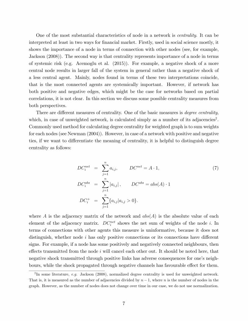
There are di§erent measures of centrality. One of the basic measures is degree centrality,
which, in case of unweighted network, is calculated simply as a number of its adjacencies2.
Commonly used method for calculating degree centrality for weighted graph is to sum weights
for each nodes (see Newman (2004)). However, in case of a network with positive and negative
ties, if we want to di§erentiate the meaning of centrality, it is helpful to distinguish degree
centrality as follows:
DCneti =nX
j=1
ai;j; DCnet = A * 1; (7)
DCabsi =nX
j=1
jai;jj ; DCabs = abs(A) * 1
DC+i =nX
j=1
fai;jjai;j > 0g:
where A is the adjacency matrix of the network and abs(A) is the absolute value of each
element of the adjacency matrix. DCneti shows the net sum of weights of the node i: In
terms of connections with other agents this measure is uninformative, because it does not
distinguish, whether node i has only positive connections or its connections have di§erent
signs. For example, if a node has some positively and negatively connected neighbours, then
e§ects transmitted from the node i will cancel each other out. It should be noted here, that
negative shock transmitted through positive links has adverse consequences for oneís neigh-
bours, while the shock propagated through negative channels has favourable e§ect for them.
2In some literature, e.g. Jackson (2008), normalized degree centrality is used for unweighted network.
That is, it is measured as the number of adjacencies divided by n) 1; where n is the number of nodes in thegraph. However, as the number of nodes does not change over time in our case, we do not use normalization.
7

In terms of systemic risk contribution net degree centrality represents the net immediate ef-
fect on iís neighbours, that is negative e§ects of the shock on iís neighbours minus a positive
one. DCabsi takes into account the absolute values of strengths of relations, therefore, it is
valid to measure connectedness with its adjacent nodes without separating them as positive
and negative relations. Absolute degree centrality gives total e§ect on neighbours in case of
shock transmission. In other words, it shows total impact of a node on the adjacent ones. To
measure only positive connections, we use DC+i , which allows to capture strength of positive
relations and shows importance of a node in terms of consequences of a negative shock on
oneís neighbours .
If we want to identify the agents who are central in terms of connections with others,
we can specify a measure of connectedness. The sum of the absolute weights measures
total involvement into connectedness of the network but does not take into consideration the
number of the edges of each node. To show this problem letís consider an example illustrated
by the Figure 1. Let node 1 connect only with node 2 with the value of connectedness w1;2 = 7
and let node 3 have Öve neighbours and let strength of connectedness with each of them be
equal to 1. The degree centrality3 of the node 1 according to the last equation (7) exceeds
the degree centrality of the node 3. It is intuitively clear that the node 3 is more central
compared to the number of neighbours perspective. So it is of important to take into account
both sum of weights and the number of neighbors when calculating the node centrality.
Opsahl, Agneessens, Skvoretz (2010) proposed using tuning parameter ? to measure
centrality which determines preference of number of edges over nodeís weights. Formally,
they use the following measure of degree centrality:
DCtunei = k1"/i %DC/i : (8)
Here ki is the number of adjacencies of the node i and DCi is one of the introduced degree
centralities above. It should be noted that the equation (8) coincides with the equations in
(7) with ? = 1; and ? = 0 gives us the number of edges of node, ki. In other words DCtunei
measures degree centrality giving more value to the weights of node with ? close to one and
it gives more value to the number of edges with ? close to zero. See Table 1 for the example
comparing DC and DCtune.
The other measure of centrality is eigenvector centrality. It characterizes centrality of a
node based on the neighborsí centrality. Again, it is possible to distinguish this centrality
measure in terms of connections with others and in terms of systemic risk, but before that
let brieáy look at the idea of eigenvector centrality in general.
3As in our example we do not use edges with negative weights, the introduced degree centrality measures
coincide.
8
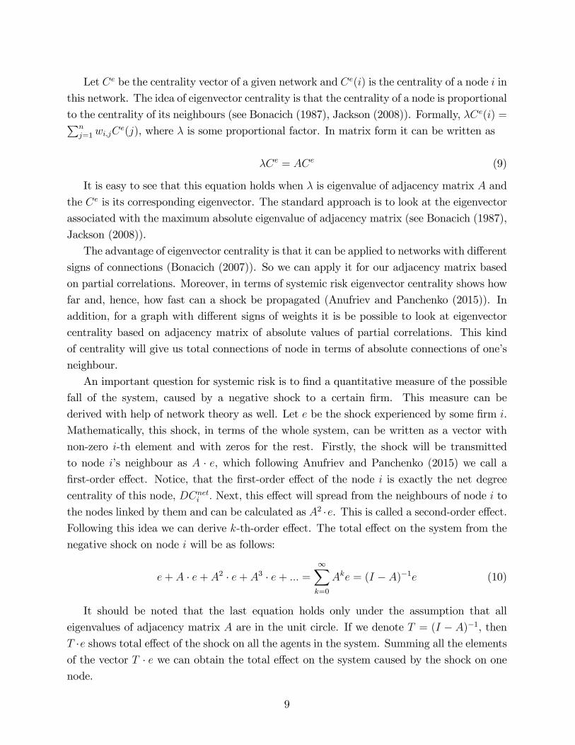
Let Ce be the centrality vector of a given network and Ce(i) is the centrality of a node i in
this network. The idea of eigenvector centrality is that the centrality of a node is proportional
to the centrality of its neighbours (see Bonacich (1987), Jackson (2008)). Formally, @Ce(i) =Pn
j=1wi;jCe(j), where @ is some proportional factor. In matrix form it can be written as
@Ce = ACe (9)
It is easy to see that this equation holds when @ is eigenvalue of adjacency matrix A and
the Ce is its corresponding eigenvector. The standard approach is to look at the eigenvector
associated with the maximum absolute eigenvalue of adjacency matrix (see Bonacich (1987),
Jackson (2008)).
The advantage of eigenvector centrality is that it can be applied to networks with di§erent
signs of connections (Bonacich (2007)). So we can apply it for our adjacency matrix based
on partial correlations. Moreover, in terms of systemic risk eigenvector centrality shows how
far and, hence, how fast can a shock be propagated (Anufriev and Panchenko (2015)). In
addition, for a graph with di§erent signs of weights it is be possible to look at eigenvector
centrality based on adjacency matrix of absolute values of partial correlations. This kind
of centrality will give us total connections of node in terms of absolute connections of oneís
neighbour.
An important question for systemic risk is to Önd a quantitative measure of the possible
fall of the system, caused by a negative shock to a certain Örm. This measure can be
derived with help of network theory as well. Let e be the shock experienced by some Örm i.
Mathematically, this shock, in terms of the whole system, can be written as a vector with
non-zero i-th element and with zeros for the rest. Firstly, the shock will be transmitted
to node iís neighbour as A * e, which following Anufriev and Panchenko (2015) we call aÖrst-order e§ect. Notice, that the Örst-order e§ect of the node i is exactly the net degree
centrality of this node, DCneti : Next, this e§ect will spread from the neighbours of node i to
the nodes linked by them and can be calculated as A2 *e. This is called a second-order e§ect.Following this idea we can derive k-th-order e§ect. The total e§ect on the system from the
negative shock on node i will be as follows:
e+ A * e+ A2 * e+ A3 * e+ ::: =1X
k=0
Ake = (I ) A)"1e (10)
It should be noted that the last equation holds only under the assumption that all
eigenvalues of adjacency matrix A are in the unit circle. If we denote T = (I ) A)"1, thenT *e shows total e§ect of the shock on all the agents in the system. Summing all the elementsof the vector T * e we can obtain the total e§ect on the system caused by the shock on one
node.
9

It has been shown that Bonacich centrality with C = 1 is linked with total e§ect matrix T
(Anufriev and Panchenko (2015)). Indeed, Bonacich centrality, also known as beta-centrality,
is calculated as
CB(C) =
1X
k=1
Ck"1Ak * 1 = (I ) CA)"1A * 1
In case of C = 1 beta-centrality
CB(1) = A * 1 + A2 * 1 + A3 * 1 + ::: = T * 1) 1 (11)
Equation 11 shows cumulative e§ect from the Örst-order of a unit shock e = 1: It is easy
to see that beta-centrality shows total e§ect of the shock minus the value of this shock. In
other words, it measures the value of consequences of shocks of each node separately. It
should be noted again that to apply this measure eigenvalues of the adjacency matrix ought
to be inside unit circle.
It is of interest to look at macro characteristics of the network such as number of edges,
diameter and average path length of the network in dynamics. The number of edges is simply
the number of the connections in our network. The diameter is the largest path between
any two nodes. In other words it shows maximum steps needed for the shock on one node to
reach the other nodes. The average path length measures the average shortest path between
nodes, so it shows the average number of steps of shock propagation in terms of network.
All three characteristics are strongly related: the average path length is bounded above by
the diameter and coincides with it in case of a fully connected network (that is when all
nodes are interconnected); the more the number of the edges in the network the less average
path length and diameter. In other words, the more connected a network is the more is
the number of edges in it and the less are the diameter and average path length. We will
look at these characteristics over time to see at which periods our network was more or less
connected.
Moreover, it is of importance to deÖne the periods when system in general was more
vulnerable. In order to do so, we calculate the average of Bonacich centrality measures with
C = 1 at each time. To distinguish the possibility that larger Örms may cause larger falls,
we also consider Bonacich centralities weighted with capitalization of assets of each Örm.
These measures can help to compare conditions of Önancial systems over the time in terms
of sensitivity to negative externalities.
10
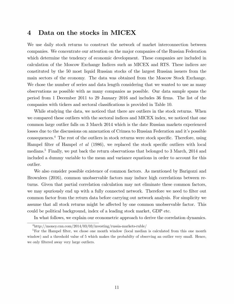
4 Data on the stocks in MICEX
We use daily stock returns to construct the network of market interconnection between
companies. We concentrate our attention on the major companies of the Russian Federation
which determine the tendency of economic development. These companies are included in
calculation of the Moscow Exchange Indices such as MICEX and RTS. These indices are
constituted by the 50 most liquid Russian stocks of the largest Russian issuers from the
main sectors of the economy. The data was obtained from the Moscow Stock Exchange.
We chose the number of series and data length considering that we wanted to use as many
observations as possible with as many companies as possible. Our data sample spans the
period from 1 December 2011 to 29 January 2016 and includes 36 Örms. The list of the
companies with tickers and sectoral classiÖcations is provided in Table 10.
While studying the data, we noticed that there are outliers in the stock returns. When
we compared these outliers with the sectoral indices and MICEX index, we noticed that one
common large outlier falls on 3 March 2014 which is the date Russian markets experienced
losses due to the discussions on annexation of Crimea to Russian Federation and itís possible
consequences.4 The rest of the outliers in stock returns were stock speciÖc. Therefore, using
Hampel Ölter of Hampel et al (1986), we replaced the stock speciÖc outliers with local
medians.5 Finally, we put back the return observations that belonged to 3 March, 2014 and
included a dummy variable to the mean and variance equations in order to account for this
outlier.
We also consider possible existence of common factors. As mentioned by Barigozzi and
Brownlees (2016), common unobservable factors may induce high correlations between re-
turns. Given that partial correlation calculation may not eliminate these common factors,
we may spuriously end up with a fully connected network. Therefore we need to Ölter out
common factor from the return data before carrying out network analysis. For simplicity we
assume that all stock returns might be a§ected by one common unobservable factor. This
could be political background, index of a leading stock market, GDP etc.
In what follows, we explain our econometric approach to derive the correlation dynamics.
4http://money.cnn.com/2014/03/03/investing/russia-markets-ruble/5For the Hampel Ölter, we chose one month window (local median is calculated from this one month
window) and a threshold value of 5 which makes the probabilty of observing an outlier very small. Hence,
we only Öltered away very large outliers.
11

5 Econometric Models
In our paper we use the correlations obtained from constant conditional correlations GARCH
(CCC-GARCH) model of Bollerslev (1990) and consistent dynamic conditional correlations
GARCH (cDCC-GARCH) model of Aielli (2008). We construct our equations as follows.
5.1 Conditional Mean
We deÖne rt to be a kx1 vector of return series, then the return equation is given by:
rt = D1 + D2Outt + Crt"1 + cft + "t (12)
ft = ,ft"1 + !t "t
!t
!v N
0k;
"Ht 0
0 )
#!
where C is a kxk matrix, D1; D2 and c are kx1 vectors and c and , are scalar parameters,
Outt is a dummy that stands for the outliers and ft is an unobserved factor. "t and !t are
assumed to be orthogonal, hence we have a linear state space form. This is a VAR(1) model
that considers a dummy variable for outliers and also includes an unobserved latent variable.
We assume that there is only one factor for simplicity.
5.2 Conditional Variance
Conditional variance of the errors "t in the conditional mean equation is given by Ht such
that:
"t = H1=2t vt (13)
Ht = DtRtDt
Dt = diag(h1=21t ; h
1=22t ; :::; h
1=2kt )
ht+1 = W1 +W2Outt + A"(2)t +Bht
where the conditional variance Ht is decomposed into a diagonal matrix of conditional
volatilities ht and correlation matrix Rt. W1 and W2 are kx1 vectors; A and B are diagonal
kxk matrix of parameters. Hence for each series i, the corresponding volatility equation is:
hi;t+1 = w1i + w2iOutt + ai"(2)i;t + bihi;t
12

The conditional variances, hi;t are positive as long as parameters w1i > 0, w2i > 0, ai > 0and bi > 0 for all i, which is a su¢ciency condition. On the other hand hi;t are stationarywhen ai + bi < 1.
5.3 Conditional Correlation
We consider two conditional correlation models, depending on how the conditional correlation
matrixRt. The Örst and simplest one is the Constant Conditional Correlation GARCHmodel
of Bollerslev (1990) where the correlation matrix is constant overtime, i :e Rt = R. This
constant correlation matrix tells us the correlation between the returns over all the sample
periods hence will help us to have a general look at the network connections between Örms
and sectors.
The second speciÖcation we consider is the cDCC-GARCH model of Aielli (2008) which
extends the correlation equation of CCC-GARCH model by deÖning correlation dynamics
as follows:
Rt = PtQtPt (14)
Pt = diag(Qt)"1=2
Qt+1 = (1) R1 ) R2)Q+ R1S$tS$0t + R2Qt
!$t = diag(Qt)1=2!t:
St = D"1t "t
where Q is replaced in the estimation by S; the sample covariance of the S$t . This is
referred to as the correlation targeting approach (Engle, 2009) and it reduces signiÖcantly
the number of parameters to be estimated. R1 and R2 are non-negative parameters which
satisfy R1 + R2 < 1. Using the correlation estimates of the cDCC-GARCH model, we can
derive the correlations between Örms and sectors at each period, and therefore we can have
a look at the network connections on a particular date: for example before and after a shock
that a§ected MICEX index.
6 Estimation
Given that we consider many series and therefore we have many parameters to estimate,
we estimate our models in three steps: Örst mean equation parameters, then volatility para-
meters and then correlation parameters. Gaussian three-step estimators are consistent and
asymptotically normal. Monte Carlo simulations in Carnero and Eratalay (2014) show that
they behave well in small samples.
13
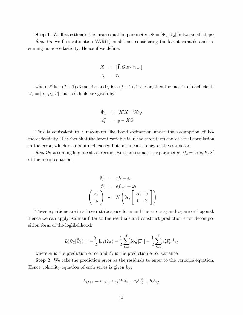
Step 1. We Örst estimate the mean equation parameters * = [*1;*2] in two small steps:Step 1a: we Örst estimate a VAR(1) model not considering the latent variable and as-
suming homoscedasticity. Hence if we deÖne:
X = [~1; Outt; rt"1]
y = rt
where X is a (T )1)x3 matrix, and y is a (T )1)x1 vector, then the matrix of coe¢cients*1 = [D1; D2; C] and residuals are given by:
*1 = [X 0X]"1X 0y
"$t = y )X*
This is equivalent to a maximum likelihood estimation under the assumption of ho-
moscedasticity. The fact that the latent variable is in the error term causes serial correlation
in the error, which results in ine¢ciency but not inconsistency of the estimator.
Step 1b: assuming homoscedastic errors, we then estimate the parameters*2 = [c; p;H;)]
of the mean equation:
"$t = cft + "t
ft = ,ft"1 + !t "t
!t
!v N
0k;
"Ht 0
0 )
#!
These equations are in a linear state space form and the errors "t and !t are orthogonal.
Hence we can apply Kalman Ölter to the residuals and construct prediction error decompo-
sition form of the loglikelihood:
L(*2j*1) = )T
2log(2Y))
1
2
TX
t=2
log jFtj )1
2
TX
t=2
e0tF"1t et
where et is the prediction error and Ft is the prediction error variance.
Step 2. We take the prediction error as the residuals to enter to the variance equation.Hence volatility equation of each series is given by:
hi;t+1 = w1i + w2iOutt + aie(2)i;t + bihi;t
14

Given that there are no volatility spillovers, we can estimate the conditional variance
parameters 3i = fw1i;w2i;ai; big of each return series i univariately by maximizing: thefollowing loglikelihood with respect to 3i:
L(3ij*) = )T
2log(2Y))
TX
t=2
loghi;t )1
2
TX
t=2
S2i;t
where vi;t = ei;t=phi;t are the standardized errors corresponding to series i:
Step 3. We estimate the correlation dynamics following the composite likelihood methoddiscussed in Engle, Sheppard and Shephard (2008). This is equivalent to a classical maximum
likelihood method for estimating the volatilities and correlations of a CCC-GARCH model.
However when estimating the correlation parameters of DCC and cDCC-GARCH models
with high number of series, Engle and Sheppard (2001) and later Engle, Sheppard and
Shephard (2008) noted that attenuation biases are observed in the R parameters of equation
(14), resulting in smoother correlation estimates. For very high number of series, the estimate
of the underlying correlation is close to being constant and equal to the long-run matrix.
This might lead the researchers to assume that the conditional correlations in the data is
constant over time. Composite likelihood method solves this problem by choosing small
subsamples, evaluating the loglikelihood of these subsamples and taking an average over
these loglikelihoods.6
If we would call 4 = fR1; R2g the correlation parameters, taking vi;t = ei;t=qhi;t from the
Örst two steps, we can estimate the correlation matrix of a CCC-GARCH model by:
R = corr(vt) =
Pvi;tvj;tPv2i;tPv2j;t
For the estimation of the cDCC-GARCH model, we take * and 3 from the Örst two
steps and we choose subsamples from k series. These subsamples can be chosen as all
subsequent series such as {{1,2},{2,3},...{k-1,k}}, or all possible bivariate combinations. It
is also possible to choose trivariate subsamples as well. In our paper, we use all possible
bivariate combinations. We also allow for di§erent dynamics for the correlations between
Örms of the same sector, with parameters 41 and of di§erent sectors 42. Hence if the chosen
subsample comes from same sector the corresponding correlation parameter vector is 41; if
not, then it is 42.
In the this stage we choose all bivariate combinations as subsamples and we construct
the loglikelihood of these subsamples:
ls = )1
2
TX
t=2
)log jRtj+ bS 0tR"1
t bSt+
(15)
6Hafner and Reznikova (2010) suggest, as another approach, the use of shrinkage methods to solve this
problem.
15
and we maximize the following loglikelihood with respect to 4 = [41;42]:
L(4j*; 3) =1
N
Xls
After obtaining 4, a forward recursion based on equation (14) using all series would
provide the conditional correlation estimates, Rt.
Although this three step procedure is not e¢cient, it still provides consistent and asymp-
totically normal estimators. (See Engle, Sheppard, Shephard 2008).
7 Empirical Part
The network analysis as we described above can be applied in di§erent cases to examine
connectedness. In this section we apply this approach to study the connectedness between
major Örms in Russia.
7.1 Constant correlations
Constant correlation matrix R is estimated as correlations between standardized residuals
in CCC-GARCH model. Using equation (5) we obtain an estimate of constant partial cor-
relation matrix. Figure 2 displays histogram of ordinary correlations and partial correlation
coe¢cients and borders of conÖdence interval for partial correlations around zero.7 It can
be seen that although there are no negative correlations, some partial correlations can be
negative. However the majority of partial correlations are positive.
The network based on GGM is depicted on the Figure 3. Only signiÖcant partial cor-
relations are used. Positive relationships between Örms are indicated with solid lines while
negative relationships are denoted by red dashed lines.
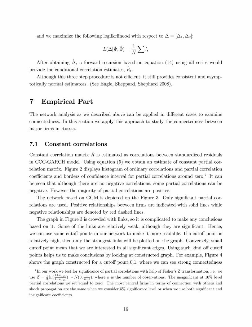
The graph in Figure 3 is crowded with links, so it is complicated to make any conclusions
based on it. Some of the links are relatively weak, although they are signiÖcant. Hence,
we can use some cuto§ points in our network to make it more readable. If a cuto§ point is
relatively high, then only the strongest links will be plotted on the graph. Conversely, small
cuto§ point mean that we are interested in all signiÖcant edges. Using such kind o§ cuto§
points helps us to make conclusions by looking at constructed graph. For example, Figure 4
shows the graph constructed for a cuto§ point 0.1, where we can see strong connectedness
7In our work we test for signiÖcance of partial correlations with help of Fisherís Z transformation, i.e. we
use Z = 12 ln(
1+!i;jj:1#!i;jj:
) , N(0; 1n#3 ), where n is the number of observations. The insigniÖcant at 10% level
partial correlations we set equal to zero. The most central Örms in terms of connection with others and
shock propagation are the same when we consider 5% signiÖcance level or when we use both signiÖcant and
insigniÖcant coe¢cients.
16

within some sectors such as Oil&Gas sector and Power sector. Moreover, we can note that
in this graph there are clusters between some Örms from Oil&Gas sector and Metal&Mining
sector. Of course, it is just a suggestion based on the constructed graph by eliminating
relatively small links, but we can check, whether it is true for the graph based on all signiÖcant
partial correlations by calculating weights within sectors.
In the Table 2 we summarize network characteristics based on sectors. Firstly, we calcu-
lated the number of Örms in each sector and the total number of links within sectors. It is not
surprising that among the largest companies in Russia: 8 belong to the Oil&Gas sector and
7 - to Metal&Mining sector. Also the sum of weights within sectors was calculated. To com-
pare calculated existence and strength of connectedness between all sectors these measures
should be normalized by the number of possible connectedness within each sector. Columns
Av.edge and Av.weights show normalized number of edges and sum of weights respectively.
Calculation of connectedness within sectors suggests that there are strong connectedness
within Power sector while Oil&Gas sector is slightly less connected than Power and Finan-
cial sectors. Moreover, in terms of presence of connections, the Oils&Gas, Metal&Mining,
Financial and Power sectors are similarly connected.
It is of interest to identify central players both in terms of connection with other Örms and
shock propagation in case of constant correlations model. We use centrality measurements
discussed in Section 3. In Table 3 centrality measures are provided for the top twelve compa-
nies according to the Bonacich centrality (CB), which represents top systemic contributors.
There k is the number of neighbors of the companies, DCnet; DCabs; DC+ are the degree
centralities discussed in (7). We also calculate eigenvector centrality, EC; to show how far
and how fast the shock of the Örm can spread in the system. In order to compare di§erent
measures of connectedness we also use degree centrality (DCtune) measure suggested by Op-
sahl, Agneessens, Skvoretz (2010) with tuning parameter ? = 0:5 and eigenvector centrality
based on the adjacency matrix of absolute weights between nodes, ECabs: We normalize
both eigenvector centralities setting the largest component of each to 1 and sort the whole
table in descending order of the Bonacich centrality. The order according to each measure
is provided in the parentheses on the right side of the value.
The table shows that the most central Örms in Russian Stock Market in terms of con-
nection with others are Sberbank (SBER) and Lukoil (LKOH), while the most systemic risk
contributors are FGC UES (FEES) and Gazprom (GAZP). It is interesting that the FGC
UES (FEES) has less connections with others (e.g. DCabsand DCtune suggest it), but it has
highest Bonacich and eigenvector centralities. It happens because FGC UES (FEES) has
the strongest connection with the ROSSETI (RSTI), which makes propagation of the shock
from FGC UES (FEES) faster and riskier for the system.
17
7.2 Dynamic correlations
CCC-GARCH model gives us a constant network of connections in Russian Stock Market.
It is well known that Russia faced a number of problems during 2014, such as devaluation
of ruble and trade sanctions imposed by European Union and Russian Federation, and it
can be said that 2014 was a year of Önancial and economic distress for Russia. During this
period some of the Örms su§ered more than others due to, for example, stronger sensitivity
to áuctuations in exchange rate and oil prices. Therefore, it would be a strong assumption,
if we suggest that correlations between stock returns remained the same throughout all time.
Hence, we are interested in examining how the connectedness between stocks changed over
time, especially during the crisis. To do that we use cDCC-GARCHmodel to obtain dynamic
correlation matrix Rt; which we use to calculate partial correlation matrix at each time t.
The methodology remains the same as in the constant correlation case except that we
now can look at changes of macro characteristics of the networks. In Figure 5 we present
changes in the number of signiÖcant edges and the average path length that we discussed in
Section 3. We calculate average path length for the graph of absolute weights to look at the
total connectedness of the network.
We can see that both the number of connections and the average path length change
over time at the graph. Moreover, we see that in 2014 the former increases while the latter
declines. This Ögure shows us that during the crisis the connectedness in Russian Stock
Market strengthens. Similar results were obtained by Diebold and Yilmaz (2014) for U.S.
stock market in the Önancial crisis 2007-2008.
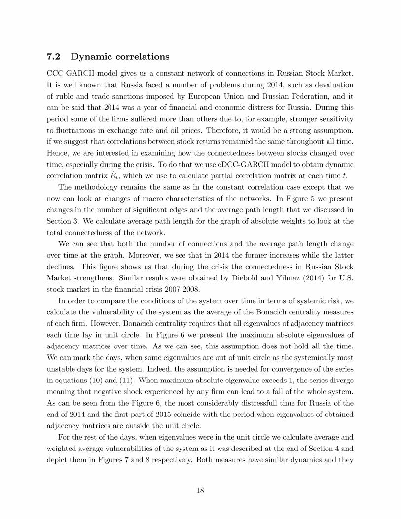
In order to compare the conditions of the system over time in terms of systemic risk, we
calculate the vulnerability of the system as the average of the Bonacich centrality measures
of each Örm. However, Bonacich centrality requires that all eigenvalues of adjacency matrices
each time lay in unit circle. In Figure 6 we present the maximum absolute eigenvalues of
adjacency matrices over time. As we can see, this assumption does not hold all the time.
We can mark the days, when some eigenvalues are out of unit circle as the systemically most
unstable days for the system. Indeed, the assumption is needed for convergence of the series
in equations (10) and (11). When maximum absolute eigenvalue exceeds 1, the series diverge
meaning that negative shock experienced by any Örm can lead to a fall of the whole system.
As can be seen from the Figure 6, the most considerably distressfull time for Russia of the
end of 2014 and the Örst part of 2015 coincide with the period when eigenvalues of obtained
adjacency matrices are outside the unit circle.
For the rest of the days, when eigenvalues were in the unit circle we calculate average and
weighted average vulnerabilities of the system as it was described at the end of Section 4 and
depict them in Figures 7 and 8 respectively. Both measures have similar dynamics and they
18
show that vulnerability of the system changes over time rising during restless periods. The
highest values are reached in the summer of 2012, that is at that time Russian stock market
was considerably sensitive to the shock propagation. We should note that eigenvalues at
these days reached their local maximum. Also it can be seen that before the marked risky
days these measures were higher than usual indicating the coming of the most systemically
unstable days.
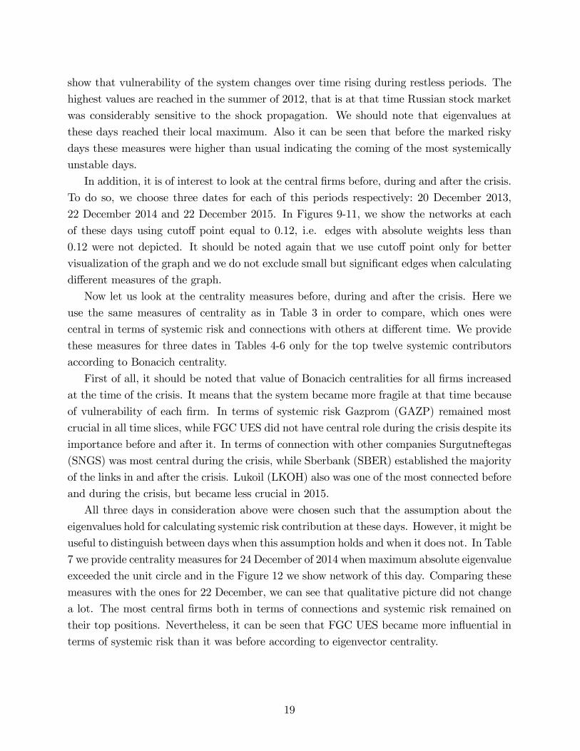
In addition, it is of interest to look at the central Örms before, during and after the crisis.
To do so, we choose three dates for each of this periods respectively: 20 December 2013,
22 December 2014 and 22 December 2015. In Figures 9-11, we show the networks at each
of these days using cuto§ point equal to 0.12, i.e. edges with absolute weights less than
0.12 were not depicted. It should be noted again that we use cuto§ point only for better
visualization of the graph and we do not exclude small but signiÖcant edges when calculating
di§erent measures of the graph.
Now let us look at the centrality measures before, during and after the crisis. Here we
use the same measures of centrality as in Table 3 in order to compare, which ones were
central in terms of systemic risk and connections with others at di§erent time. We provide
these measures for three dates in Tables 4-6 only for the top twelve systemic contributors
according to Bonacich centrality.
First of all, it should be noted that value of Bonacich centralities for all Örms increased
at the time of the crisis. It means that the system became more fragile at that time because
of vulnerability of each Örm. In terms of systemic risk Gazprom (GAZP) remained most
crucial in all time slices, while FGC UES did not have central role during the crisis despite its
importance before and after it. In terms of connection with other companies Surgutneftegas
(SNGS) was most central during the crisis, while Sberbank (SBER) established the majority
of the links in and after the crisis. Lukoil (LKOH) also was one of the most connected before
and during the crisis, but became less crucial in 2015.
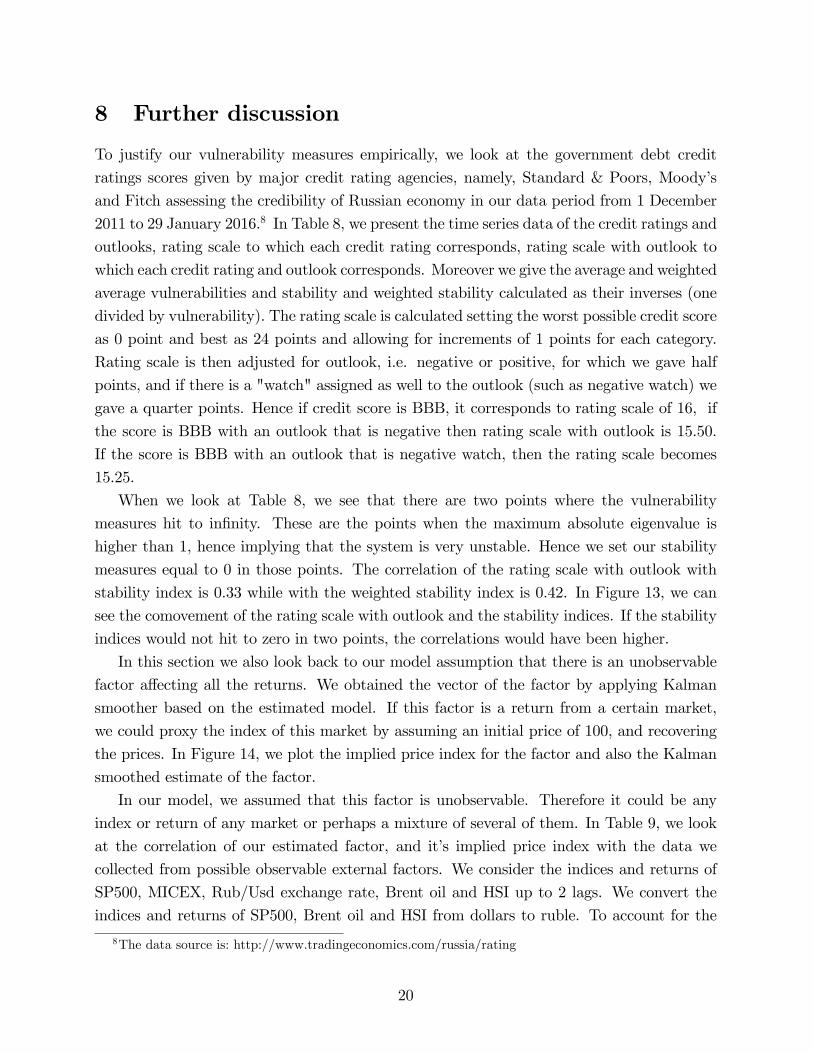
All three days in consideration above were chosen such that the assumption about the
eigenvalues hold for calculating systemic risk contribution at these days. However, it might be
useful to distinguish between days when this assumption holds and when it does not. In Table
7 we provide centrality measures for 24 December of 2014 when maximum absolute eigenvalue
exceeded the unit circle and in the Figure 12 we show network of this day. Comparing these
measures with the ones for 22 December, we can see that qualitative picture did not change
a lot. The most central Örms both in terms of connections and systemic risk remained on
their top positions. Nevertheless, it can be seen that FGC UES became more ináuential in
terms of systemic risk than it was before according to eigenvector centrality.
19
8 Further discussion
To justify our vulnerability measures empirically, we look at the government debt credit
ratings scores given by major credit rating agencies, namely, Standard & Poors, Moodyís
and Fitch assessing the credibility of Russian economy in our data period from 1 December
2011 to 29 January 2016.8 In Table 8, we present the time series data of the credit ratings and
outlooks, rating scale to which each credit rating corresponds, rating scale with outlook to
which each credit rating and outlook corresponds. Moreover we give the average and weighted
average vulnerabilities and stability and weighted stability calculated as their inverses (one
divided by vulnerability). The rating scale is calculated setting the worst possible credit score
as 0 point and best as 24 points and allowing for increments of 1 points for each category.
Rating scale is then adjusted for outlook, i.e. negative or positive, for which we gave half
points, and if there is a "watch" assigned as well to the outlook (such as negative watch) we
gave a quarter points. Hence if credit score is BBB, it corresponds to rating scale of 16, if
the score is BBB with an outlook that is negative then rating scale with outlook is 15.50.
If the score is BBB with an outlook that is negative watch, then the rating scale becomes
15.25.
When we look at Table 8, we see that there are two points where the vulnerability
measures hit to inÖnity. These are the points when the maximum absolute eigenvalue is
higher than 1, hence implying that the system is very unstable. Hence we set our stability
measures equal to 0 in those points. The correlation of the rating scale with outlook with
stability index is 0.33 while with the weighted stability index is 0.42. In Figure 13, we can
see the comovement of the rating scale with outlook and the stability indices. If the stability
indices would not hit to zero in two points, the correlations would have been higher.
In this section we also look back to our model assumption that there is an unobservable
factor a§ecting all the returns. We obtained the vector of the factor by applying Kalman
smoother based on the estimated model. If this factor is a return from a certain market,
we could proxy the index of this market by assuming an initial price of 100, and recovering
the prices. In Figure 14, we plot the implied price index for the factor and also the Kalman
smoothed estimate of the factor.
In our model, we assumed that this factor is unobservable. Therefore it could be any
index or return of any market or perhaps a mixture of several of them. In Table 9, we look
at the correlation of our estimated factor, and itís implied price index with the data we
collected from possible observable external factors. We consider the indices and returns of
SP500, MICEX, Rub/Usd exchange rate, Brent oil and HSI up to 2 lags. We convert the
indices and returns of SP500, Brent oil and HSI from dollars to ruble. To account for the
8The data source is: http://www.tradingeconomics.com/russia/rating
20

risk consider the VIX index which is the implied volatility of the SP500, Morgan Stanley
Composite index for Emerging Markets (MSCIEM) and for world markets (MSCIW). The
latter two we converted from dollars to rubles. Finally, we also considered the Economic
Policy Uncertainty Index for Russia.9 This data is monthly, so we took the monthly mean
and median of the factor, to check for correlation.
From Table 9, we can see that, there are many cases where the correlations are positive
and signiÖcant. In particular, the factor is signiÖcantly positively correlated with the SP500
returns (in rubles), HSI returns (in rubles) and also with the Usd/Rub exchange rate returns,
but not with the squares of these series. The factor is also signiÖcantly positively correlated
with the MSCIEM and MSCIW indices. The monthly mean and median series of the factor
is signiÖcantly positively correlated with the changes in the economic policy uncertainty.
Finally, the implied prices of the factor is signiÖcantly positively correlated with the price
levels and indices of many of the external factors we considered. Interestingly the correlation
with VIX index is not signiÖcant, but the squared factor is correlated with the VIX index.
On the other hand, the factor is signiÖcantly negatively correlated with the squared returns
of Brent oil (in rubles) and with its two periods past values.
9 Conclusion
In this paper we mapped the most liquid and major Örms in Russian Stock Market (MICEX)
bringing together the ideas from Önancial econometrics, Gaussian graphical model and net-
work analysis. More speciÖcally, we derived partial correlations from the correlation esti-
mates of constant conditional correlation (CCC) and consistent dynamic conditional correla-
tion (DCC) GARCH models. Further using Gaussian graphical model approach, we derived
the undirected weighted connections between the stocks. We examined the dynamics of
some key network measures such as number of edges in graph and average path length and
centrality. In addition, we distinguished centrality measures between two types: centrality
as connectedness with others and centrality as importance for systemic risk. Given that we
had connections with negative weights, these two centrality measures implied di§erent re-
sults. We found that the most connected Örms are Sberbank and Lukoil, while most central
in terms of systemic risk are Gazprom and FGC UES.
On the other hand, using the Bonacich centralities of the stocks, we came up with two
measures of vulnerability of the system: the Örst one is the average of Bonacich centralities,
and the second - is the weighted average of Bonacich centralities. For the weights, we consid-
ered market capitalization of the stocks on each day. We deÖned the inverse of vulnerability
9Data source: http://www.policyuncertainty.com/
21

as the system stability index. It turns out that the stability indices discussed in our arti-
cle represent comovement and positive correlation with the government debt credit ratings
reported by major credit rating agencies, namely Standard & Poors, Moodyís and Fitch.
Our article can be extended in various ways. First of all, one could include more stocks of
Önancial companies and banks to the data series. Then one can discuss the Önancial stability
of the system. On the other hand, one could run vector autoregressions with vulnerability
series and some external factors such as oil prices and exchange rates, to derive the impulse
response functions. In this way, one could see how the system vulnerability would react to
shocks introduced to these series.
10 Acknowledgements
We are very grateful to Mikhail Anufriev, Valentyn Panchenko and Maxim Bouev for very
useful comments. Also, we thank the participants of a department seminar in European
University at St. Petersburg. All remaining errors are ours.
References
[1] Acemoglu, D., Ozdaglar, A., Tahbaz-Salehi, A. (2015). Systemic risk and stability in
nancial networks. American Economic Review 105, 564-608.
[2] Adrian, T., Brunnermeier, M.K. (2016). CoVaR. American Economic Review,106(7):
1705-1741.
[3] Anufriev, M., Panchenko, V., (2015). Connecting the dots: Econometric methods for
uncovering networks with an application to the Australian Önancial institutions. Journal
of Banking and Finance, Vol. 61, S241-S255
[4] Aielli, G. P. (2008). Consistent estimation of large scale dynamic conditional corre-
lations. Unpublished paper: Department of Economics, Statistics, Mathematics and
Sociology, University of Messina. Working paper n. 47.
[5] Barigozzi, M., Brownlees, C. (2016). NETS: Network Estimation for Time Series. Work-
ing Paper. Barselona Graduate School of Economics.
[6] Bauwens, L., Laurent, S. and J.V.K. Rombouts (2006). Multivariate GARCH Models:
A Survey. Journal of Applied Econometrics, 21, 79-109.
[7] Bonacich, P.(1987). Power and centrality: A family of measures. American journal of
sociology, 1170-1182.
22
[8] Bonacich, P. (2007). Some unique properties of eigenvector centrality. Social Network,
555-564.
[9] Bollerslev, T. (1990). Modelling the Coherence in Short-Run Nominal Exchange Rates:
A Multivariate Generalized ARCH Model. The Review of Economics and Statistics, 72,
498-505.
[10] Bollerslev, T. (1986). Generalized Autoregressive Conditional Heteroskedasticity, Jour-
nal of Econometrics, 31:307-327
[11] Borovkova, S., Lopuhaa, R. (2012). Spatial GARCH: A spatial approach to multivariate
volatility modelling. Available at SSRN 2176781.
[12] Brownlees, C., Engle, R. (2016). SRISKS: A Conditional Capital Shortfall Measure of
Systemic Risk. Working Paper.
[13] Brownlees, C., Hans, C., Nualart, E. (2014). Bank Credit Risk Networks: Evidence
from the Eurozone Crisis. Working Paper.
[14] Buhlmann.P., Van De Geer, S. (2011). Statistics for High-Dimensional Data: Methods,
Theory and Applications. Springer.
[15] Carnero, A., Eratalay, M.H. (2014). Estimating VAR-MGARCH Models in Multiple
Steps, Studies in Nonlinear Dynamics and Econometrics, Vol 18, 3.
[16] Diebold, F. X., Yilmaz, K. (2009), Measuring Önancial asset return and volatilty
spillovers, with application to global equity markets, The Economic Journal, Vol. 119,
Issue 534, 158-171.
[17] Diebold, F. X., Yilmaz, K. (2014), On the network topology of variance decompositions:
Measuring the connectedness of Önancial Örms, Journal of Econometrics, 182-1, 119-
134.
[18] Engle, R., N. Shephard and K. Sheppard (2008). Fitting and Testing Vast Dimensional
Time-Varying Covariance Models. NYU Working Paper No. FIN-07-046.
[19] Engle, R. (2002). Dynamic Conditional Correlation: A Simple Class of Multivariate
Generalized Autoregressive Conditional Heteroskedasticity Models. Journal of Business
and Economic Statistics, 20, 339-350.
[20] Engle, R., K. Sheppard (2001). Theoretical and Empirical Properties of Dynamic Con-
ditional Correlation Multivariate GARCH. NBER Working Paper, No: W8554.
23
[21] Engle, R. (1982). Autoregressive Conditional Heteroscedasticity with Estimates of Vari-
ance of United Kingdom Ináation, Econometrica 50:987-1008.
[22] Hafner C.M. and Reznikova, O. (2010) On the estimatiion of dynamic conditional cor-
relation models, Computational Statistics and Data Analysis, forthcoming.
[23] Hampel, F. R., Ronchetti, E. M., Rousseeuw, P. J., Stahel, W. A. (1986). Robust
Statistics: The Approach Based on Ináuence Functions. Wiley, New York.
[24] Hastie, T., Tibshirani, R., Friedman, J. (2009). The Elements of Statistical Learning.
Volume 2. Springer.
[25] Jackson, M.O. (2008). Social and Economic Networks. Princeton University Press.
[26] Krumsiek, J., Suhre, K., Illing, T., Theis, F., J., Adamski J. (2011). Gaussian graphi-
cal modeling reconstructs pathway reaction from high-throughput metabolomics data.
BMC Systems Biology, 5-21
[27] Kunegis, J., Lommatzsch, A., Bauckhage, C. (2009). The Slashdot Zoo: Mining a Social
Network with Negative Edges. Proceedings of the 18th international conference onWorld
wide web, 741-750.
[28] Newman, M.E.J. (2004) Analysis of weighted networks. Physical Review E 70, 056131.
[29] Opsahl, T., Agneessens, F., Skvoretz, J. (2010). Node centrality in weighted networks:
Generalizing degree and shortest paths. Social Networks 32, 245-251.
[30] Rice, J.,J., Tu, Y., Stolovitzky, G. (2005). Reconstructing biological networks using
conditional correlation analysis. Bioinformatics 21, 765-773.
[31] Silvennoinen, A. and T. Ter‰svirta (2009). Multivariate GARCH Models. In T. G.
Andersen, R. A. Davis, J.-P. Kreiss and T. Mikosch, eds. Handbook of Financial Time
Series. New York: Springer.
[32] Weiss, Y., Freeman, W. T. (1999). Correctness of Belief Propagation on Gaussian
Graphical Models of Arbitrary Topology. Neural Computation, Vol. 13, No. 10, 2173-
2200.
24
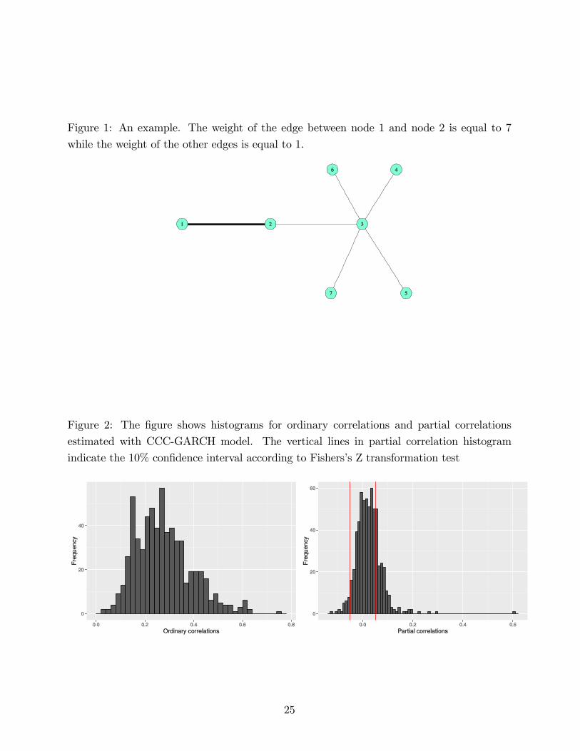
Figure 1: An example. The weight of the edge between node 1 and node 2 is equal to 7
while the weight of the other edges is equal to 1.
Figure 2: The Ögure shows histograms for ordinary correlations and partial correlations
estimated with CCC-GARCH model. The vertical lines in partial correlation histogram
indicate the 10% conÖdence interval according to Fishersís Z transformation test
25

Figure 3: Network constructed using Gaussian Graphical Model. Network shows the bidi-
rectional connectedness between major Örms in Russian listed in MOEX. Nodes colored by
the sectors. Solid lines between nodes denote positive conditional dependences between cor-
responding pairs while red dashed line denote negative relations. The thicker the line the
stronger connection.
Figure 4: Network with cuto§ point equal to 0.1
26
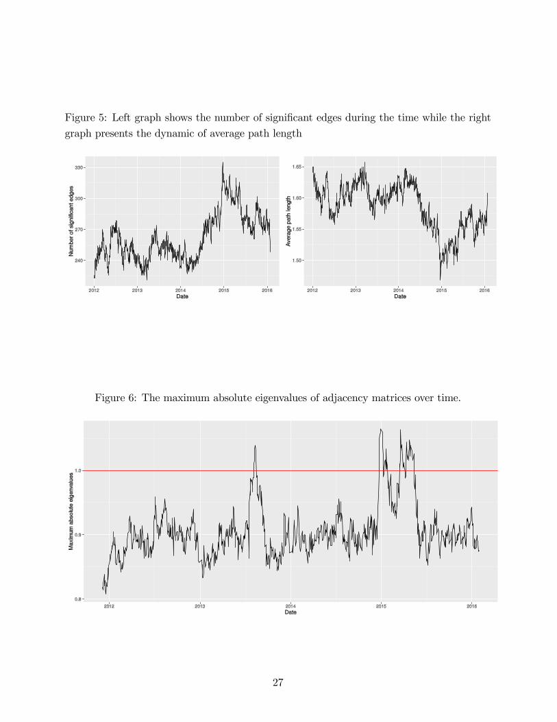
Figure 5: Left graph shows the number of signiÖcant edges during the time while the right
graph presents the dynamic of average path length
Figure 6: The maximum absolute eigenvalues of adjacency matrices over time.
27

Figure 7: Average vulnerability of the system. It was calculated as the average of the
Bonacich centralities of the nodes at each time
Figure 8: Weighted average vulnerability of the system. Weights were taken as the market
capitalization weights among considered Örms
28

Figure 9: Network of 20 December 2013
Figure 10: Network of 22 December 2014
29
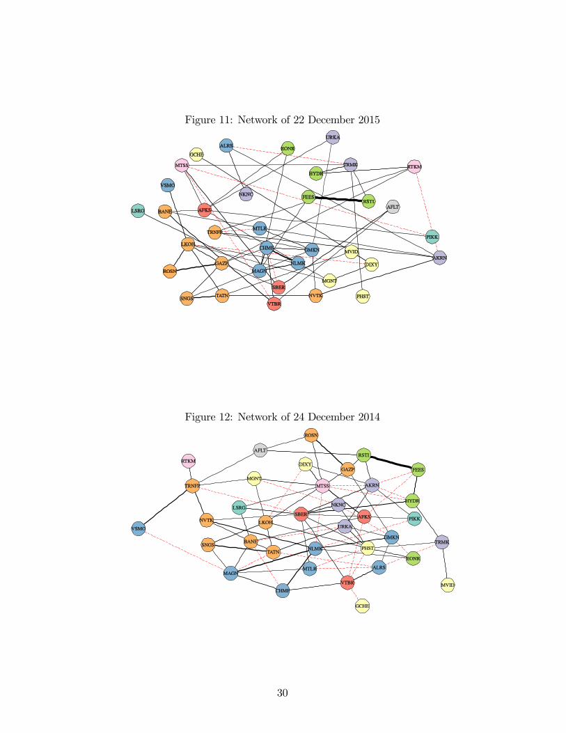
Figure 11: Network of 22 December 2015
Figure 12: Network of 24 December 2014
30

Figure 13: Rating scales with outlook (based on the credit ratings of major agencies on
Russian economy) vs. the stability indices (calculated based on the vulnerability indices).
31
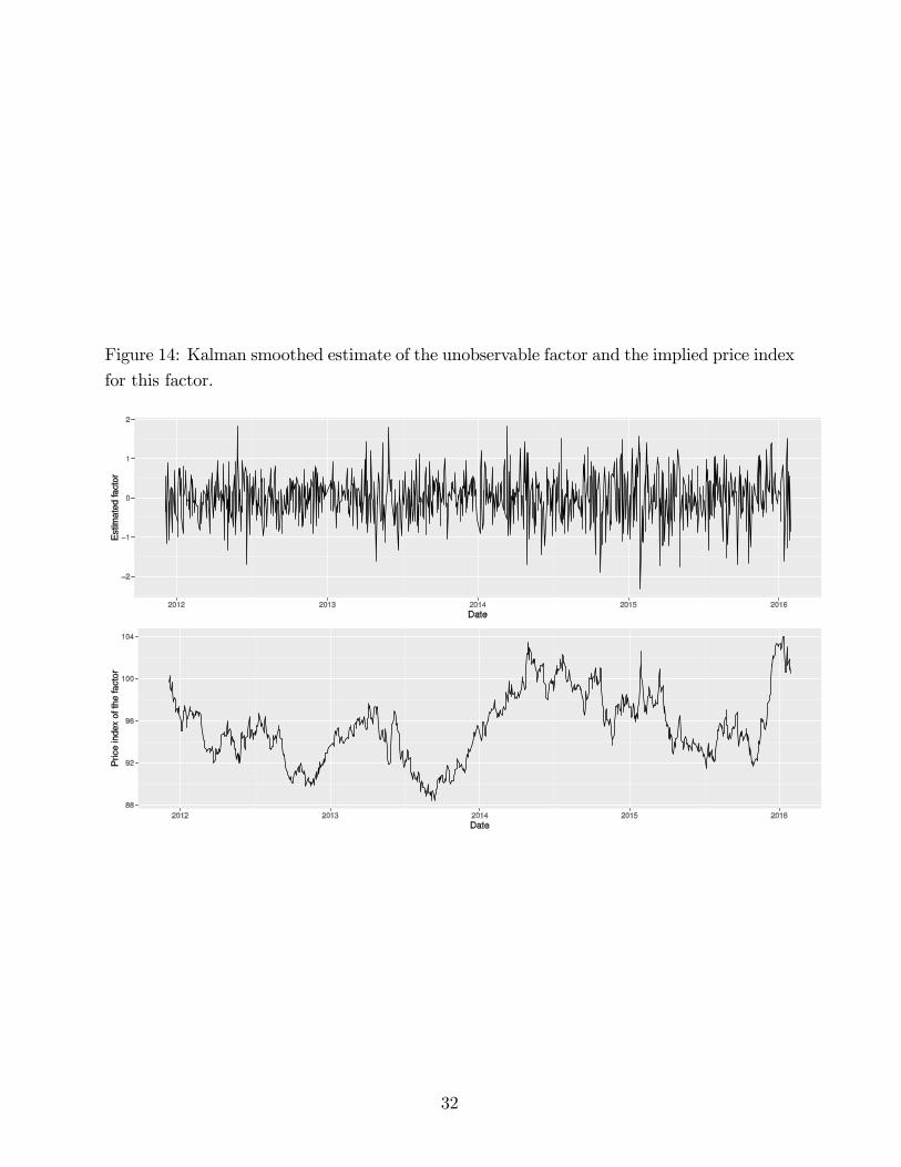
Figure 14: Kalman smoothed estimate of the unobservable factor and the implied price index
for this factor.
32

Table 1: Example
Node k DC DCtune
1 1 7 2.65
2 2 8 4
3 6 6 6
DCtunei with ( = 0:5
Table 2: Within sector calculations
Sector # Örms # edges sum of weights # negative Av.edges Av.weights
O&G 8 17 1.9 0 0.6 0.068
M&M 7 13 1.2 2 0.62 0.057
CGS 5 4 0.344 0 0.4 0.034
PWR 4 4 0.938 0 0.667 0.156
CHM 4 2 0.022 1 0.333 0.004
FNL 3 2 0.27 0 0.667 0.09
C&D 2 1 0.087 0 1 0.087
TLC 2 1 0 0 0 0
TRN 1 0 0 0 - -
Columns indicate from left to right, tickers of the sectors, number of edges within the sector, net sum of
weights in the sector, number of negative edges within the sector, average number of edges equal to the
number of edges divided by the number of possible edges within the sector, and average weights are the sum
of weights divided by the number of all possible edges.
33

Table 3: Centrality Measures
k DCnet DCabs DC+ DCtune EC ECabs CB
FEES 7 1.147 (10) 1.147 (10) 1.147 (5) 2.833 (20) 1.000 (1) 0.999 (2) 7.487 (1)
GAZP 12 1.200 (2) 1.200 (7) 1.200 (3) 3.795 (6) 0.895 (2) 0.889 (4) 7.337 (2)
NLMK 11 1.159 (8) 1.159 (8) 1.159 (4) 3.571 (7) 0.760 (5) 0.776 (9) 6.449 (3)
RSTI 10 0.856 (11) 1.223 (4) 1.040 (9) 3.497 (8) 0.877 (3) 1.000 (1) 6.378 (4)
LKOH 16 1.040 (6) 1.478 (1) 1.259 (2) 4.863 (2) 0.764 (4) 0.999 (3) 6.326 (5)
SNGS 15 1.082 (5) 1.204 (5) 1.143 (6) 4.249 (3) 0.724 (6) 0.869 (6) 6.111 (6)
TATN 14 0.927 (7) 1.279 (3) 1.103 (7) 4.232 (4) 0.693 (8) 0.886 (5) 5.764 (7)
SBER 17 1.202 (1) 1.464 (2) 1.333 (1) 4.988 (1) 0.635 (11) 0.731 (11) 5.737 (8)
CHMF 10 0.863 (10) 1.152 (9) 1.007 (10) 3.394 (9) 0.694 (7) 0.815 (8) 5.705 (9)
MAGN 12 0.897 (8) 1.201 (6) 1.049 (8) 3.797 (5) 0.650 (9) 0.832 (7) 5.378 (10)
ROSN 9 0.771 (15) 0.957 (11) 0.864 (11) 2.934 (16) 0.638 (10) 0.774 (10) 5.185 (11)
NVTK 12 0.863 (9) 0.863 (16) 0.863 (12) 3.218 (12) 0.555 (12) 0.542 (15) 4.763 (12)
This table shows calculated di§erent centrality measures for top twelve companies according to Bonacich
centrality in the case of constant model. Here k is the number of adjacencies of the node; DCnet; DCabs; DC+
are net degree centrality, degree centrality of adjacency matrix with absolute values, positive degree centrality
measures respectively; DCtune is tuned degree centrality with ( = 0:5; EC and ECabs are eigenvector
centrality for adjacency matrix and adjacency matrix with absolute values and CB is Bonacich centrality
with + = 1:
Table 4: Centrality Measures. 20.12.2013
k DCnet DCabs DC+ DCtune EC ECabs CB
FEES 12 1.102 (6) 1.646 (5) 1.374 (3) 4.444 (13) 1.000 (1) 1.000 (1) 9.501 (1)
GAZP 14 1.132 (4) 1.407 (14) 1.269 (9) 4.438 (14) 0.796 (3) 0.709 (13) 8.974 (2)
LKOH 16 1.130 (5) 1.675 (4) 1.402 (2) 5.177 (6) 0.709 (5) 0.866 (4) 8.252 (3)
SNGS 20 1.165 (2) 1.820 (1) 1.492 (1) 6.032 (1) 0.715 (4) 0.882 (3) 8.209 (4)
NLMK 12 1.168 (1) 1.472 (12) 1.320 (6) 4.203 (19) 0.647 (8) 0.743 (11) 7.954 (5)
RSTI 13 0.853 (14) 1.607 (6) 1.230 (11) 4.571 (11) 0.870 (2) 0.944 (2) 7.914 (6)
SBER 17 1.133 (3) 1.567 (8) 1.350 (4) 5.162 (7) 0.629 (10) 0.721 (12) 7.576 (7)
CHMF 12 1.014 (8) 1.478 (11) 1.246 (10) 4.211 (17) 0.614 (11) 0.768 (8) 7.512 (8)
ROSN 13 0.888 (11) 1.267 (18) 1.077 (15) 4.058 (22) 0.665 (7) 0.696 (14) 7.382 (9)
HYDR 18 1.050 (7) 1.524 (10) 1.287 (8) 5.237 (5) 0.672 (6) 0.743 (10) 7.227 (10)
MAGN 19 0.950 (10) 1.699 (3) 1.324 (5) 5.681 (3) 0.581 (12) 0.850 (5) 7.009 (11)
TATN 17 0.726 (17) 1.554 (9) 1.140 (14) 5.139 (8) 0.636 (9) 0.779 (7) 6.965 (12)
34
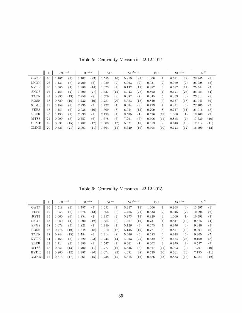
Table 5: Centrality Measures. 22.12.2014
k DCnet DCabs DC+ DCtune EC ECabs CB
GAZP 16 1.407 (3) 1.702 (23) 1.555 (10) 5.219 (25) 1.000 (1) 0.621 (22) 28.245 (1)
LKOH 26 1.131 (7) 2.709 (2) 1.920 (2) 8.393 (2) 0.931 (2) 0.959 (2) 25.928 (2)
NVTK 20 1.366 (4) 1.880 (14) 1.623 (7) 6.132 (11) 0.887 (3) 0.687 (14) 25.544 (3)
SNGS 16 1.485 (2) 1.590 (27) 1.537 (12) 5.043 (28) 0.862 (4) 0.621 (23) 25.084 (4)
TATN 21 0.893 (13) 2.259 (8) 1.576 (9) 6.887 (7) 0.845 (5) 0.833 (8) 23.614 (5)
ROSN 18 0.829 (16) 1.732 (19) 1.281 (20) 5.583 (18) 0.820 (6) 0.637 (18) 23.041 (6)
NLMK 19 1.159 (6) 2.295 (7) 1.727 (4) 6.604 (9) 0.799 (7) 0.871 (6) 22.705 (7)
FEES 18 1.181 (5) 2.036 (10) 1.609 (8) 6.054 (13) 0.709 (8) 0.747 (11) 21.016 (8)
SBER 25 1.493 (1) 2.893 (1) 2.193 (1) 8.505 (1) 0.596 (12) 1.000 (1) 18.760 (9)
MTSS 22 0.999 (8) 2.357 (6) 1.678 (6) 7.201 (6) 0.606 (11) 0.855 (7) 17.639 (10)
CHMF 18 0.831 (15) 1.787 (17) 1.309 (17) 5.671 (16) 0.613 (9) 0.648 (16) 17.314 (11)
GMKN 20 0.725 (21) 2.003 (11) 1.364 (15) 6.329 (10) 0.608 (10) 0.723 (12) 16.590 (12)
Table 6: Centrality Measures. 22.12.2015
k DCnet DCabs DC+ DCtune EC ECabs CB
GAZP 16 1.518 (1) 1.787 (5) 1.652 (1) 5.347 (11) 1.000 (1) 0.968 (4) 13.597 (1)
FEES 12 1.055 (7) 1.676 (13) 1.366 (6) 4.485 (21) 0.833 (2) 0.946 (7) 10.696 (2)
RSTI 15 1.060 (6) 1.854 (2) 1.457 (3) 5.273 (14) 0.829 (3) 1.000 (1) 10.591 (3)
LKOH 13 1.080 (4) 1.690 (12) 1.385 (5) 4.687 (19) 0.731 (4) 0.847 (15) 9.875 (4)
SNGS 18 1.078 (5) 1.821 (3) 1.450 (4) 5.726 (4) 0.675 (7) 0.976 (3) 9.340 (5)
ROSN 16 0.776 (19) 1.648 (18) 1.212 (17) 5.135 (16) 0.721 (5) 0.871 (12) 9.294 (6)
TATN 18 0.844 (15) 1.784 (6) 1.314 (8) 5.666 (6) 0.683 (6) 0.948 (6) 9.205 (7)
NVTK 14 1.165 (2) 1.322 (23) 1.244 (14) 4.303 (25) 0.632 (8) 0.664 (25) 9.169 (8)
SBER 22 1.114 (3) 1.980 (1) 1.547 (2) 6.601 (1) 0.602 (9) 0.979 (2) 8.547 (9)
MTSS 18 0.851 (13) 1.702 (11) 1.277 (12) 5.536 (8) 0.527 (11) 0.903 (9) 7.297 (10)
HYDR 13 0.860 (12) 1.287 (26) 1.074 (22) 4.091 (28) 0.539 (10) 0.661 (26) 7.195 (11)
GMKN 17 0.815 (17) 1.661 (15) 1.238 (15) 5.315 (12) 0.486 (13) 0.833 (16) 6.984 (12)
35

Table 7: Centrality Measures. 24.12.2014
k DCnet DCabs DC+ DCtune EC ECabs
GAZP 17 1.401 (2) 1.833 (20) 1.617 (5) 5.582 (20) 1.000 (1) 0.640 (19)
LKOH 23 1.179 (6) 2.538 (3) 1.859 (2) 7.640 (3) 0.916 (2) 0.862 (3)
FEES 20 1.191 (5) 2.243 (7) 1.717 (3) 6.698 (8) 0.897 (3) 0.790 (6)
NVTK 20 1.275 (4) 1.908 (16) 1.592 (7) 6.178 (13) 0.831 (4) 0.651 (18)
TATN 22 0.852 (9) 2.294 (6) 1.573 (9) 7.104 (5) 0.803 (5) 0.783 (7)
SNGS 14 1.363 (3) 1.466 (29) 1.414 (14) 4.531 (31) 0.787 (6) 0.526 (27)
ROSN 19 0.824 (11) 1.904 (18) 1.364 (16) 6.015 (16) 0.778 (7) 0.656 (16)
NLMK 18 1.143 (7) 2.187 (9) 1.665 (4) 6.275 (12) 0.744 (8) 0.763 (9)
RSTI 16 0.766 (17) 2.066 (13) 1.416 (13) 5.750 (19) 0.693 (9) 0.744 (11)
SBER 24 1.539 (1) 2.991 (1) 2.265 (1) 8.472 (1) 0.645 (10) 1.000 (1)
HYDR 18 0.703 (21) 1.905 (17) 1.304 (19) 5.856 (17) 0.577 (11) 0.674 (15)
MGNT 14 0.779 (16) 1.397 (33) 1.088 (27) 4.422 (32) 0.541 (12) 0.487 (34)
Table 8: Credit ratings history
Agencies Credit rating Outlook Dates R.S. R.S., out Avg. Vuln. W. Avg. Vuln. Stability W. Stab.
Fitch BBB stable 16.01.2012 16.00 16.00 6.71 9.19 0.15 0.11
S&P BBB negative 20.03.2014 16.00 15.50 4.22 5.37 0.24 0.19
Fitch BBB negative 21.03.2014 16.00 15.50 5.58 6.63 0.18 0.15
Moodyís Baa1 neg. watch 28.03.2014 17.00 16.25 4.87 6.74 0.21 0.15
S&P BBB- negative 25.04.2014 15.00 14.50 7.83 11.36 0.13 0.09
Moodyís Baa1 negative 27.06.2014 17.00 16.50 5.73 7.83 0.17 0.13
Moodyís Baa2 negative 17.10.2014 16.00 15.50 7.59 10.70 0.13 0.09
S&P BBB- neg. watch 23.12.2014 15.00 14.25 Inf Inf 0 0
Fitch BBB- negative 09.01.2015 15.00 14.50 4.38 6.61 0.23 0.15
Moodyís Baa3 neg. watch 16.01.2015 15.00 14.25 Inf Inf 0 0
S&P BB+ negative 26.01.2015 14.00 13.50 5.05 7.62 0.20 0.13
Moodyís Ba1 negative 20.02.2015 14.00 13.50 7.95 12.32 0.13 0.08
Moodyís Ba1 stable 03.12.2015 14.00 14.00 6.22 9.05 0.16 0.11
36

Table 9: Pearson correlations between the smoothed factor and external data.
Series Corr(.,factor) Series Corr(.,factor)
SP500 returns (in rub) 0:0862(0:0053)
SP500 (in rub) sq. 0:0286(0:3555)
MICEX returns "0:0000(0:9991)
MICEX sq. "0:0300(0:3327)
USD/RUB returns 0:0932(0:0026)
USD/RUB sq. 0:0018(0:9549)
BRENT returns (in rub) "0:0123(0:6910)
BRENT (in rub) sq. "0:0772(0:0127)
HSI returns (in rub) 0:1114(0:0003)
HSI returns (in rub) sq. "0:0005(0:9878)
SP500 returns (in rub) (-1) 0:0059(0:8481)
SP500 returns (in rub) (-1) sq. "0:0101(0:7437)
MICEX returns (-1) "0:0655(0:0345)
MICEX returns (-1) sq. 0:0240(0:4382)
USD/RUB returns (-1) 0:0113(0:7147)
USD/RUB returns (-1) sq. 0:0262(0:3984)
BRENT returns (in rub) (-1) "0:0464(0:1342)
BRENT returns (in rub) (-1) sq. "0:0013(0:9659)
HSI returns (in rub) (-1) "0:0102(0:7431)
HSI returns (in rub) (-1) sq. 0:0343(0:2686)
SP500 returns (in rub) (-2) 0:0217(0:4848)
SP500 returns (in rub) (-2) sq. "0:0295(0:3414)
MICEX returns (-2) 0:0541(0:0813)
MICEX returns (-2) sq. 0:0407(0:1897)
USD/RUB returns (-2) 0:0450(0:1469)
USD/RUB returns (-2) sq. "0:0397(0:2007)
BRENT returns (in rub) (-2) 0:0038(0:9028)
BRENT returns (in rub) (-2) sq. "0:0660(0:0333)
HSI returns (in rub) (-2) 0:0341(0:2716)
HSI returns (in rub) (-2) sq. "0:0329(0:2896)
VIX "0:0292(0:3461)
VIX (-1) "0:0219(0:4810)
VIX vs squared factor 0:1181(0:0001)
VIX vs squared factor (-1) 0:1135(0:0002)
MSCIEM* (in rub) 0:0939(0:0029)
MSCIW* (in rub) 0:0892(0:0077)
Unc. ind. vs monthly mean f. 0:1142(0:4298)
Ch. in unc. ind. vs monthly mean f. 0:2305(0:1111)
Unc. ind. vs monthly med. f. 0:1969(0:1705)
Ch. in unc. ind. vs monthly med. f. 0:2648(0:0660)
SP500 ind. (rub) vs factor price 0:3136(0:0000)
USD/RUB levels vs factor price 0:2901(0:0000)
MICEX index vs factor price 0:0507(0:1015)
BRENT price (rub) vs factor price 0:2152(0:0000)
HSI index vs factor price 0:0405(0:1914)
MSCIEM* index (rub) vs factor price 0:3284(0:0000)
MSCIW* index (rub) vs factor price 0:3394(0:0000)
37

Table 10: Stocks listed in MICEX with corresponding sector information
Ticker Name S. Index Sector
AFKS AFK SISTEMA FNL Financial
AFLT JSC "AEROFLOT" TRN Transport
AKRN Acron CHM Chemicals
ALRS AC "ALROSA" M&M Metals and mining
BANE OAO ANK "Bashneft" O&G Oil and gas
CHMF Severstal M&M Metals and mining
DIXY DIXY Group CGS Consumer goods and services
EONR OAO "E.ON Rossiya" PWR Electricity, utilities
FEES "FGC UES" JSC PWR Electricity, utilities
GAZP GAZPROM O&G Oil and gas
GCHE PJSC "Cherkizovo Group" CGS Consumer goods and services
GMKN "OJSC" MMC "NORILSK NICKEL" M&M Metals and mining
HYDR JSC "RusHydro" PWR Electricity, utilities
LKOH OAO "LUKOIL" O&G Oil and gas
LSRG OJSC LSR Group C&D Construction and development
MAGN OJSC "MMK" M&M Metals and mining
MGNT OJSC "Magnit" CGS Consumer goods and services
MTLR Mechel OAO M&M Metals and mining
MTSS MTS OJSC TLC Telecommunications
MVID Open Joint-Stock Company "M.video" CGS Consumer goods and services
NKNC PJSC "Nizhnekamskneftekhim" CHM Chemicals
NLMK NLMK M&M Metals and mining
NVTK JSC "NOVATEK" O&G Oil and gas
PHST JSC "Pharmstandard" CGS Consumer goods and services
PIKK "PIK Group" C&D Construction and development
ROSN Rosneft O&G Oil and gas
RSTI PJSC "ROSSETI" PWR Electricity, utilities
RTKM Rostelecom TLC Telecommunications
SBER Sberbank FNL Financial
SNGS Surgutneftegas O&G Oil and gas
TATN TATNEFT O&G Oil and gas
TRMK TMK CHM Chemicals
TRNFP Transneft Pref. O&G Oil and gas
URKA Uralkali CHM Chemicals
VSMO VSMPO-AVISMA Corporation M&M Metals and mining
VTBR JSC VTB Bank FNL Financial38