Mapping Properties of BacklundTransformations and the AsymptoticStability of Soliton Solutions for theNonlinear Schrodinger and Modified

Korteweg-de-Vries Equation

Dissertationzur

Erlangung des Doktorgrads (Dr. rer. nat.)der

Mathematisch-Naturwissenschaftlichen Fakultatder

Rheinischen Friedrich-Wilhelms-Universitat Bonn

vorgelegt vonStefan Korner

ausLeverkusen

Bonn, 2019

Angefertigt mit Genehmigung der Mathematisch-NaturwissenschaftlichenFakultat der Rheinischen Friedrich-Wilhelms-Universitat Bonn

1. Gutachter: Prof. Dr. Herbert Koch2. Gutachter: Prof. Dr. Juan J. L. Velazquez

Tag der Promotion: 31.01.2020

Erscheinungsjahr: 2020

Acknowledgements

First, I want to express my gratitude to Prof. Herbert Koch, who has been avery dedicated advisor and without whose guidance, suggestions and (some-times) patience this thesis would not have been possible.

Second, I thank my wonderful parents, Barbara Korner and Dr. WilfriedKorner, for their loving support throughout the past years, as well as myother family and friends.

Third, I thank Prof. Martin Rumpf, who agreed to be my mentor at theBonn International Graduate School of Mathematics (BIGS) when I startedout, and has always given me kind but clear words of advice. I also extendmy thanks to Prof. Juan Velazquez and Prof. Thomas Martin, as well asProf. Rumpf, for agreeing to be part of the doctoral committee.

My final word of gratitude goes out to the past and present members of theresearch group ”Analysis and Partial Differential Equations” at the Univer-sity of Bonn. It has been a genuine pleasure to meet, interact with and workalongside all of them.

1

Summary

We consider the cubic Nonlinear Schrodinger Equation (NLS) and the Mod-ified Korteweg-de-Vries Equation (mKdV) in the one-dimensional, focusingcase. For the mKdV, we also restrict ourselves to the case of real-valuedsolutions. The Lax formalism for the Nonlinear Schrodinger Hierarchy givesrise to a Backlund transformation, which connects the trivial zero solutionto the elementary soliton solution for both equations.

Following an approach pioneered by Mizumachi and Pelinovsky, this the-sis uses the Backlund transformation to prove asymptotic stability of NLS-and mKdV-solitons by showing that known stability properties of the zerosolution transfer to the solitons. An important feature of the argument pre-sented here is that it proceeds by relatively elementary techniques, withoutinvoking the Riemann-Hilbert-formalism of inverse scattering theory.

For the essential asymptotic stability of the zero solution, we will invokeresults by Ifrim and Tataru and by Harrop-Griffiths, which also provideasymptotic expressions for the potentials under consideration. This willenable us to understand the behaviour of the Jost solutions for the corre-sponding Lax systems as the time t→∞. Our asymptotic stability resultscontain time-dependent position, and in the NLS case, phase shift functions,which we will show to converge to constant values as t → ∞ on the basisof these findings. It is a particularly notable point that we will be ableto show quantitative estimates for how fast position and phase will go totheir respective limits. In the mKdV case, we will actually be able to showconvergence properties of the Jost solutions beyond what is necessary forour stability arguments, which could potentially be useful in applying themethods of this thesis to other special mKdV-solutions.

A large portion of the arguments given should generalize to other equa-tions in the NLS hierarchy, provided a suitable asymptotic stability resultfor the zero solution is available.

2

Contents

1 Introduction 4

2 The Stability Problem for special NLS and mKdV Solutions 8

3 The NLS Hierarchy and the Backlund Transformation 12

4 Properties of Jost Solutions 18

5 Asymptotic Stability of the NLS Soliton Solutions 29

6 The mKdV Case 59

Bibliography 78

3

Chapter 1

Introduction

The family of Nonlinear Schrodinger Equations is used to model a wide vari-ety of wave phenomena, ranging from the theory of water waves to nonlinearoptics (compare e.g. [2], [10], [17]). In the following we will concern our-selves with the initial value problem for the one-dimensional, cubic, focusingequation

iut + uxx + 2|u|2u = 0, (1.1)

with u = u(t, x) : R+×R→ C a complex-valued function with u(0, ·) = u01.

Unless otherwise indicated, we will use the abbreviation ”NLS” exclusivelyto refer to this case.

The formalism of inverse scattering theory, originally developed in [1], givesrise to a map that will send any solution of NLS to another solution of thesame equation, called a Backlund transformation. Backlund transformationsare intimately connected to a class of particle-like solutions called solitons.In [22], Mizumachi and Pelinovsky used the Backlund transformation forNLS to show L2-stability of soliton solutions. Their proof was based onreduction of the problem to the L2-stability of the zero solution (which isknown by conversation of L2-energy). There are also several asymptotic sta-bility results for the zero solution available (e.g. [13], [16] and several others).It is therefore a natural question if these, too, transfer to soliton solutionsvia the Backlund transformation, which Mizumachi and Pelinovsky left openat the end of their paper. In [8], Cuccagna and Pelinovsky gave one suchproof. Their argument is partially based on an asymptotic stability resultfor the zero solution of their own, which at the same time provides greatergenerality in the sense that it applies to all pure radiation solutions. To doso, they rely on an explicit analysis of the Riemann-Hilbert problem frominverse scattering theory.

1For simplicity, we restrict ourselves to positive times t in the first argument.

4

LetH0,1(R) be the function space defined by the norm ‖f‖H0,1(R) = ‖f‖L2(R)+‖xf‖L2(R). In Theorem 5.2 of this thesis, we will give a proof of asymptoticstability of NLS solitons with initially small H0,1-norm that does not relyon analysis of the Riemann-Hilbert problem2 and thus provides a more el-ementary alternative to [8]. (It should be emphasized that, while we aregoing to restrict ourselves to H0,1(R) for simplicity, similar arguments workfor all other spaces to which Remark 2.4 applies.)

In order to achieve this (in Theorem 5.2), we will follow in the footstepsof [22] in analyzing the properties of the Jost solutions3 for the spatial partof the Lax system from inverse scattering theory (see (3.1), (3.2) and thefollowing discussion in Chapter 3):

∂x

(ψ1

ψ2

)=

(−iζ u−u iζ

)(ψ1

ψ2

), (1.2)

where ζ ∈ C with Im(ζ) > 0, ψ = ψ(x) : R → C × C (actually ψ(t, x) :R+ ×R→ C×C, considered at a fixed timepoint t ∈ R+ here), and we aremostly concerned with the case that the potential u is a solution of NLS inan appropriate function space. The Jost solutions behave like free solutionsfor potential u = 0 as x → ∞ or −∞: The left Jost solution behaves like

e−iζx(

10

)for x→ −∞, the right Jost solution like eiζx

(01

)as x→∞.

We will show that in the case of a small L∞-norm of u ∈ L2(R), the ”large”component that dominates the Jost solution at +∞ or −∞ dominates ev-erywhere, in a manner controlled by the L∞-norm. The decisive argumentsare in Proposition 5.8 and Claim 5.9, the latter of which plays a similar roleto Lemma 4.3 in [8]. While Cuccagna and Pelinovsky employ their detailedanalysis of pure radiation NLS solutions, we will use an argument that em-ploys Gronwall’s inequality and the boundedness of the Jost solutions onone side to show Claim 5.9. An interesting point to note is that Claim 5.9only depends on the L∞-smallness of the potential. Again using Gronwall’sinequality, we will utilize this result to understand a suitable sense in whichthe left and right Jost solution behave like exponential functions (see espe-cially (5.27) and (5.28)).

The arguments outlined in the previous paragraph yield a preliminary resultwhere our limit still includes time-dependent position and phase parameters,which we can characterize in terms of the absolute values of the Jost solu-tions on the real line. A particularly important feature of Theorem 5.2 isthat we show convergence (as t→∞) of these parameters with quantitative

2Another difference to [8] is how the pullback at t = 0 is established in Lemma 5.3.3Although Mizumachi and Pelinovsky define the solutions slightly differently than we

are going to do in the following. For clarification, see Remark 4.2.

5

estimates for the rate, given in (5.3) and (5.4). To do so, we will make useof [16], where Tataru and Ifrim derived an asymptotic stability result forsolutions with small H0,1-norms at t = 0 without the aid of inverse scat-tering theory, and especially, they obtained an asymptotic expression forthe solution (we give their findings in Theorem 2.3). This can be used tounderstand the behaviour of the Jost solutions as t→∞ (Lemma 5.10) andshow the desired convergence properties of position and phase.

Another nonlinear partial differential equation which admits a family of soli-ton solutions is the modified Korteweg-de-Vries equation (mKdV in the fol-lowing) which we pose for a real-valued4 function u = u(t, x) : R+×R→ R:

ut + uxxx + 2(u3)x = 0, (1.3)

where u(0, ·) = u0.

This equation, too, has an associated Lax system, with the spatial part(1.2) the same as in the NLS case. And just like for the NLS, asymptoticstability results for the zero solution are available, see [12], [14], [15]. We willemploy the main theorem from [12], in which Harrop-Griffiths showed such aresult without relying on inverse scattering theory, including an asymptoticexpression. This can be used for an asymptotic stability argument similarto the NLS case, as we will do in Theorem 6.1. While we have to treat aphase and a position shift when showing the asymptotic stability of (1.1),we only have to deal with a time dependent position shift function in themKdV case. Showing convergence of this function to a constant value ast→∞ turns out to be easier than in the proof for NLS (once again, note thequantitative estimate for the rate of convergence, in this case given by (6.2)).This is because the center of an mKdV soliton is near x = t on the real line,where Theorem 2.5 provides particularly sharp bounds. Unlike in the NLSresult Theorem 5.2, we therefore do not need to show pointwise convergenceof the Jost solutions to a ”long term profile” as t → ∞. However, suchconvergence does hold, as will be proved in Proposition 6.2. Some otherresults concerning the asymptotic stability of mKdV solitons have recentlybeen published by Chen and Liu ([5], [6]). Similarly to [8], they make useof the Riemann-Hilbert formalism and the steepest descent method. It alsoappears that their proof needs stronger assumptions than the one presentedin this thesis.

As we will discuss in Chapter 3, the systems of (1.1), (1.3) are connectedwith a multitude of other equations via the NLS hierarchy, and indeed, asignificant part of the argument presented in Chapter 5 (particularly the

4The reason we restrict ourselves to the real-valued case is that Theorem 2.5 is onlyavailable for real-valued solutions.

6

proof of Proposition 5.8) would transfer to other NLS hierarchy equationswith little modification, provided a suitable stability result for the zero solu-tion is available, and particularly if asymptotic expressions as in Theorems2.3 and 2.5 are given.

This thesis is organized as follows: The second chapter will introduce theresults for asymptotic stability of zero solutions for NLS and mKdV, aswell as give a brief introduction to the stability problem for soliton solu-tions. The third chapter will explain the NLS hierarchy and the Backlundtransformation for NLS and mKdV, while the fourth chapter will expandon some basic facts about Jost solutions we are going to need, which willimmediately put us in a position to understand some useful properties ofBacklund transformations. Chapter 5 will show asymptotic stability of theNLS soliton solution in the manner sketched above. Chapter 6 will dealwith the application of our stability arguments to mKdV and give a proofof Proposition 6.2. The latter might potentially be useful in the applicationof our methods to other mKdV solutions, such as breather solutions whichcan be constructed via two iterations of a Backlund transformation (see [19],Chapter 5).

7

Chapter 2

The Stability Problem forspecial NLS and mKdVSolutions

This chapter will provide some basic facts about the stability of soliton so-lutions. Our goal is to analyze the stability of NLS and mKdV on the lineby using Backlund transformations. This is accomplished by linking soli-ton stability to known stability theorems for the trivial zero solution. Asalready discussed in the Introduction, we will use the results from [12] and[16], which we will provide at the end of this chapter in Theorems 2.3 and 2.5.

One solution of the NLS equation:

iut + uxx + 2|u|2u = 0

is the elementary soliton

u(t, x) = eit sech(x) (2.1)

The original motivation for the theory of solitons was the observation byJohn Scott Russel in the 19th century that certain localized water waves ina narrow channel retain their form for an extended amount of time. Russeldubbed his discovery a ”wave of translation”, although the term solitarywave is more common today. It is called a soliton if it additionally retainsits form after collision with other solitary waves or radiation (see [24]). Ina nonlinear setting, a soliton is generally a solution for which (attractive)nonlinear effects and dispersion of wave solutions cancel out.

Two well-known symmetries of the NLS are under scaling

u(t, x)→ ku(k2t, kx), k ∈ R (2.2)

8

and the Galilei transform

u(t, x)→ eivx−iv2tu(t, x− 2vt), v ∈ R, (2.3)

i.e. if u is a solution, so are the above transformations of u. These symme-tries generate a whole family of soliton solutions from (2.1):

Qk,v(t, x) = k sech(k(x− vt))eivx2

+i(k2− v2

4)t, k ∈ R, v ∈ R (2.4)

A (not quite sharply defined, see [24]) conjecture or general expectation onsoliton solutions is that they exhibit stability properties, i.e. ”closeness”of a solution to a soliton at t = 0 implies closeness at any other t ∈ R+

(orbital stability) or even convergence in some function norm (asymptoticstability) - of course, the definition of ”closeness” must be specified. For(2.4), the Backlund transform was used in [22] to show orbital stability inthe following, particularly strong sense:1

Theorem 2.1. (Mizumachi/Pelinovsky) Let (k, v) ∈ R+×R. If a solu-tion u(t, x) ∈ C(R, L2(R))∩L8

loc(R, L4(R)) of the NLS equation (1.1) satis-fies ‖u(0, ·)−Qk,v(0, ·)‖L2(R) ≤ ε for sufficiently small ε, then for all t ∈ R,we have constants (k0, v0, t0, x0) ∈ R+ × R× R+ × R such that

‖u(t+ t0, ·+ x0)−Qk0,v0‖L2 . ‖u(0, ·)−Qk,v(0, ·)‖L2(R),

and

|k0 − k|+ |v − v0|+ |t0|+ |x0| . ‖u(0, ·)−Qk,v(0, ·)‖L2(R) (2.5)

holds.

Notice that the soliton that the NLS solution u in Theorem 2.1 remains”close” to is different from the soliton that it is close to at t = 0. Insteadit has, and needs to have, slightly different parameters k0, v0, t0 and x0

(which depend on the specific u under consideration), to incorporate thesymmetries (2.2) and (2.3). However, we can control the closeness of theseparameters to the original soliton parameters by (2.5). While the optimiza-tion over small t0 and x0 is, strictly speaking, unnecessary in Theorem 2.1,phase and position shifts will be relevant for our treatment of asymptoticstability.

The mKdV (for a real-valued2 function u)

ut + uxxx + 2(u3)x = 0

1Mizumachi and Pelinovsky formulate Theorem 2.1 specifically for v = 0, from whichthe statement for the full soliton group can easily be obtained by translation invarianceof integrals and additivity properties of the Galilei transform.

2The more general form for a complex-valued u is

ut + uxxx + 6|u|2ux = 0

9

has an elementary soliton solution

u(t, x) = sech(x− t) (2.6)

Similar to the NLS case, the symmetry under the scaling

u(t, x)→ ku(k3t, kx), k ∈ R (2.7)

as well as shifts in position u(t, x)→ u(t, x+x0), x0 ∈ R, generates a familyof solitons from (2.6):

Qk,x0(t, x) = k sech(kx− k3t+ x0), k ∈ R, x0 ∈ R, (2.8)

for which, again, we ask the stability question.

It is trivial that u = 0 is a solution of both NLS and mKdV. The L2-norm of any NLS and mKdV solution is conserved, as can be seen formallyby differentiating

∫|u|2dx under the integral sign ([4] and[20] are standard

references here), which establishes that the zero solution is orbitally stablein L2 in a very straightforward sense: If the initial data u(0, x) = u0 are L2-close to 0, so is u(t, x) at any time t > 0. Additionally, various asymptoticstability results for NLS exist, i.e. if u0 is close to zero in certain spaces,its L∞-norm will decay to zero as t → ∞. The formulation most relevantto this thesis is due to Ifrim and Tataru in [16] (we leave out some of theirfindings):

Definition 2.2. The function space Hr,s(R) is the closure of C∞0 (R) underthe norm ‖f‖Hr,s(R) = ‖(1 + | · |2)

r2 f(·)‖L2(R) + ‖(1 + | · |2)

s2 f(·)‖L2(R)

On H0,1(R), we mostly use the equivalent norm ‖f‖H0,1(R) = ‖f‖L2(R) +‖xf‖L2(R) for f = f(x) ∈ H0,1(R).

Theorem 2.3. (Ifrim/Tataru) There is ε > 0 such that for an initialdatum u0 ∈ H0,1(R) with ‖u0‖H0,1(R) ≤ ε, we have a unique solution u :

R+ × R → C with e−it2∂2xu ∈ C(R, H0,1(R)) of the Nonlinear Schrodinger

Equation (1.1) such that u(0, ·) = u0. This solution satisfies the estimate

‖u(t, ·)‖L∞(R) . ε|t|−12

for all t > 0. Moreover, there is an asymptotic expression

u(t, x) = t−12 ei

x2

2tW(xt

)ei log(t)|W (x

t)|2 + errx(t, x) (2.9)

with a complex-valued function W ∈ H1−Cε2(R) satisfying ‖W‖H1−Cε2 (R)

. ε

for a fixed C > 0 and errx(t, ·) ∈ OL∞(R)

((1 + t)−

34

+Cε2)∩ OL2(R)

((1 +

t)−1+Cε2)

.

10

Remark 2.4. As per Remark 1.1 in [16], an analogue to Theorem 2.3 canbe shown for initial data in all spaces H0,s(R) with s ∈ (1

2 , 1].

For the mKdV (real-valued case)

ut + uxxx + 2(u3)x = 0, (2.10)

we have by [12]:

Theorem 2.5. (Harrop-Griffiths) There is an ε > 0 such that if an initialdatum u0 ∈ H1,1(R) satisfies ‖u0‖H1,1(R) ≤ ε, there exists a unique globalsolution u(t, x) of (2.10) with u(0, ·) = u0 and3

‖u(t, ·)‖L∞(R) . εt−13 〈t−

13x〉−

14 ,

as well as asymptotics as t→∞ (with any real number ρ ∈ [0, 13(1

6 −Cε2)]):

‖t13 (t−

13x)

34u‖L∞(Ω+

ρ ) . ε ‖t16 (t−

13x)u‖L2(Ω+

ρ ) . ε (2.11)

on Ω+ρ = x > 0 : t−

13x & t2ρ, called the decaying region,

u(t, x) = t−13Q(t−

13x) + err(x), (2.12)

on the self-similar region Ω0ρ = x ∈ R : t−

13 |x| . t2ρ, where Q : R → R

with |Q| . ε is a solution of the Painleve II equation yQ − Qyy − 3Q3 = 0and

err(x) ∈ OL∞(Ω0ρ)

(εt−

12

( 56−Cε2)

)∩OL2(Ω0

ρ)

(εt−

23

( 512−Cε2)

), (2.13)

Finally, on the oscillatory region Ω−ρ = x < 0 : t−13 |x| & t2ρ:

u(t, x) = π−12 t−

13 (t−

13 |x|)−

14 ·

· Re(eiα(t,x)+ 3iσ

4π|W (t−

12 |x|

12 )|2 log(t−

12 |x|

12 )W (t−

12 |x|

12 ))

+ E(x),

(2.14)

with W ∈ H1−Cε2,1(R) a complex-valued function on the reals satisfying

‖W‖H1−Cε2,1∩L∞(R)

. ε and α(t, x) = −23 t− 1

2 |x|32 + π

4 . The error function E

satisfies the estimates

‖t13 (t−

13 |x|)

38E(x)‖L∞(Ω−ρ ) . ε, ‖t

16 (t−

13 |x|)

14E(x)‖L2(Ω−ρ ) . ε

The leading terms of the asymptotic expressions in both Theorem 2.3and Theorem 2.5 relate to analysis of the corresponding linearized equations.

3〈·〉 := (1 + | · |2)12 denotes the usual Japanese brackets.

11

Chapter 3

The NLS Hierarchy and theBacklund Transformation

In the following two chapters, we will review the basic facts associated toBacklund transformations for the Nonlinear Schrodinger hierarchy which areof interest in this thesis. This theory is standard in the relevant literature.For reference, see particularly [11], [19], [21] and also e.g. [8], [18] or [22].

Consider the following system of first order PDEs for a function1 ψ =ψ(t, x) : R+ × R→ C× C, referred to as a Lax system in the following:

∂x

(ψ1

ψ2

)=

(−iζ u−u iζ

)(ψ1

ψ2

)(3.1)

and

∂t

(ψ1

ψ2

)= i

(−2ζ2 + |u|2 ∂xu− 2iζu−∂xu+ 2iζu 2ζ2 − |u|2

)(ψ1

ψ2

)(3.2)

with a parameter ζ ∈ C and a potential u = u(t, x) : R+ × R → C. Someother ways of writing this system can be found in the literature, e.g. withparameter η := iζ, or as two equivalent Riccati equations for γ := ψ1

ψ2

(see [22]). Solutions of (3.1) and (3.2), or just solutions of (3.1), consid-ered at a fixed time t, are often referred to as wave functions. When weconsider (3.1) at a fixed time (or just in isolation as an ODE system forψ = ψ(t, x) : R→ C× C), we often suppress the t-dependence in our nota-tion.

Let us assume that a sufficiently regular solution ψ exists, so that we haveto demand interchangeability of the order of differentiation:

∂t∂xψ = ∂x∂tψ. (3.3)

1As mentioned before, we restrict ourselves to positive times for simplicity and physi-cality, which is not necessarily done in other literature on the topic.

12

From this compatibility condition, it can be shown that u must be a solutionof the NLS equation. For ∂xψ = Aψ and ∂tψ = Bψ, this is equivalent tothe zero curvature condition:

∂xB − ∂tA− [A,B] = 0, (3.4)

where [·, ·] denotes the commutator of two operators.

The previous statements hold for mKdV if we replace (3.2) by

∂t

(ψ1

ψ2

)= B(u, ζ)

(ψ1

ψ2

), (3.5)

with

B(u, ζ) =

−4iζ3 + 2iζ|u|2 − 2i Im(uxu) 4ζ2u+ 2iζux − (uxx + 2|u|2u)−4ζ2u+ 2iζux + (uxx + 2|u|2u) 4iζ3 − 2iζ|u|2 + 2i Im(uxu)

(3.6)

When u is real-valued, (3.6) reduces to:

B(u, ζ) =

(−4iζ3 + 2iζu2 4ζ2u+ 2iζux − (uxx + 2u3)

−4ζ2u+ 2iζux + (uxx + 2u3) 4iζ3 − 2iζu2

)(3.7)

This is part of a more general framework known as the (focusing) NLShierarchy. We follow [18], Appendix C in this brief outline: Suppose wehave the equation

∂x

(ψ1

ψ2

)=

(−iζ u−u iζ

)(ψ1

ψ2

), (3.8)

with potential u and parameter ζ ∈ C. We then look for a matrix B(u, ζ)such that the compatibility condition (3.3) arising from (3.8) and

∂t

(ψ1

ψ2

)= B(u, ζ)

(ψ1

ψ2

)(3.9)

is a partial differential equation for u. This will be true if we have[∂t −B(u, ζ), ∂x −

(−iζ u−u iζ

)]=

(0 ∂tu− F

−(∂tu− F ) 0

)!

= 0, (3.10)

with [A,B] = AB − BA denoting the commutator of two operators A andB and the function F being a polynomial in the derivatives of u and u.Indeed, when inserting the equations (3.8) and (3.9) into (3.3) it followsquickly that the left-hand side of (3.10) must be zero, so we would obtain

13

∂tu − F (u) = 0 as our desired partial differential equation. We make the

ansatz B(ζ, u) = βk(ζ, u) =k∑j=0

ζk−jQj(u) for k ∈ N0, where each Qj is a

2× 2 matrix in the special unitary group SU(2). By inserting this into thecommutator in (3.10), we get

∂t

(−iζ u−u iζ

)− ∂x

k∑j=0

ζk−jQj(u) +

[(−iζ u−u iζ

),

k∑j=0

ζk−jQj(u)

]!

= 0

We want to have the left side depend only on u, not ζ. To achieve this, it issufficient to demand

Q0 =

(−i 00 i

),

a recursive relation:[(−i 00 i

), Qj+1

]= ∂xQj +

[Qj ,

(0 u−u 0

)], 0 ≤ j ≤ k − 1

and that

∂xQk +

[Qk,

(0 u−u 0

)]

is off-diagonal. Thus, we can write Qk =

(−irk pk−pk irk

)with

pk+1 =i

2p′k + rku

r′k = i(pku− pku)

It can be shown that r can, for any k, be expressed as a polynomial in thederivatives of u and u. The first few steps of the recursion give r0 = 1,p0 = 0, p1 = u, r1 = 0, p2 = i

2u′, r2 = −1

2 |u|2, p3 = −1

4(u′′ + 2|u|2u),r3 = − i

4(u′u− uu′). The cases k = 2 and k = 3 correspond to the NLS andmKdV case, respectively2. (We get (3.2) by demanding u to be real-valued.)By u → −u we would have obtained the defocusing NLS hierarchy and byu→ 1 the KdV hierarchy. We note once again that the stability argumentsfor NLS and mKdV would largely transfer to any equation in the NLS hi-erarchy, provided one had the analogue of Theorem 2.3 and 2.5 for the zerosolution.

2Strictly speaking, the versions of NLS and mKdV obtained with these pk, rk arerescaled in the time parameter compared to how we have stated these equations. Wechoose simplicity over consistency in our notation here.

14

If

(ψ1

ψ2

)is a solution of (3.1) and (3.2), or respectively, (3.5) with parameter

ζ and a potential u that is a solution of NLS or mKdV (depending on the

matrix in the ”time part” of the system), then

(ψ1

ψ2

)with

ψ1 =ψ2

‖ψ‖2ψ2 = − ψ1

‖ψ‖2(3.11)

is a solution of the analogous system with parameter ζ and potential

u(t, x) = u(t, x) + 4 Im(ζ)ψ1ψ2

‖ψ‖2(3.12)

The mapping u→ u defined by (3.12) is called an (auto-)Backlund transfor-mation of u. The term ”Backlund transformation” is used in various con-texts to denote mappings between solutions of various partial differentialequations - e.g. if v is a solution of the Laplace equation and φ the (unique)holomorphic function with Re(φ) = v, the mapping v → v := Im(φ) is some-times (e.g. in [23]) referred to as a Backlund transformation for the Laplaceequation, which v solves. Indeed, since we have shown that the Lax systemfor NLS (or mKdV, respectively) is only solvable if its potential is a solutionof NLS (respectively mKdV) by (3.4). Thus, (3.12) must necessarily map asolution of the partial differential equation arising as a compability condi-tion for the Lax system to another such solution.

Writing the transformation (3.12) with potential u, parameter ζ and so-lution ψ of (3.1) and (3.2) as B(u, ζ, ψ)(t, x), we first note the elementary,but useful, property

B(u, ζ, cψ)(t, x) = B(u, ζ, ψ)(t, x), ∀c ∈ C\0 (3.13)

i.e. the transformation is invariant under multiplication of the wave functionwith a constant. Moreover, with B(u, ζ, ψ)(t, x) =: u(t, x), the Backlundtransformation satisfies the reiteration relation

u(t, x) = B(u, ζ, ψ)(t, x) (3.14)

with ψ defined by (3.11), which allows us to recover the original potentialu from u. Similarly to what we remarked following (3.1) and (3.2), we mayalso suppress the t-dependence of the Backlund transformation in the fol-lowing, whenever we consider (3.1) at a fixed time t ∈ R+ (or in isolation),or leave the (t, x)-argument out entirely in our notation.

As already discussed, our goal is to use the Backlund transformation to

15

transfer stability properties of the trivial zero solution of NLS and mKdVto the soliton solutions. For the NLS system, (3.1) and (3.2) with u = 0 andparameter ζ become:

∂x

(ψ1

ψ2

)=

(−iζ 0

0 iζ

)(ψ1

ψ2

)(3.15)

and

∂t

(ψ1

ψ2

)= i

(−2ζ2 0

0 2ζ2

)(ψ1

ψ2

)(3.16)

Now, (3.15) has a fundamental system of solutions consisting of(e−iζx

0

)(3.17)

and (0eiζx

), (3.18)

and in particular,

(e−iζx

eiζx

)is a solution. For a given initial value ψ(0, ·),

equation (3.16) is solved by ψ(t, x) =

(e−2iζ2tψ1(0, x)

e2iζ2tψ2(0, x)

). Together, this

gives one solution:

ψ(t, x) =

(e−2iζ2te−iζx

e2iζ2teiζx

)

of (3.15) and (3.16). If ζ = i2

(k + iv

)with k ∈ R+, v ∈ R, plugging this ψ

and u = 0 into (3.12) gives the solution

Qk,v(t, x) = k sech(k(x− vt))eivx2

+i(k2− v2

4)t,

recovering the soliton group (2.4). Similarly, we obtain the soliton group(2.8) for mKdV from the solution

ψ(t, x) =

(e−4iζ3te−iζx

e4iζ3teiζx

)

if −2iζ = k ∈ R+. In particular, notice that for ζ = i2 , we get mappings

of the zero function to the elementary soliton solutions (2.1) and (2.6) (andmost basically, the hyperbolic secant function sech(·) at t = 0).

16

As shown in [3], if a parameter ζ is not already an eigenvalue for potentialu, it will be for the Backlund transformed potential u, i.e. the effect of theBacklund transformation on the spectrum is that of inserting an eigenvalue.(”Eigenvalue” to be understood in the sense that there is an L2-solution ψ

of (3.1), which would be an ζ-eigenfunction of the operator i

(∂x −u−u −∂x

).)

For the cases close to a soliton solution that interest us, the existence of L2

eigenfunctions can be shown more explicitly (cf. [22], Lemma 3.1), and wewill elaborate on this in the next chapter.

More generally, if we just consider the spatial part of the Lax system (at afixed time, suppressing the time variable), a potential u(·) ∈ H1(R) wouldsatisfy lim

R→∞‖u‖L∞(|x|>R) = 0, i.e. we might expect the system to behave

like (3.15) as the space variable |x| → ∞. This leads one to seek solutionsthat behave like (3.17) or (3.18) at +∞ or −∞, called Jost solutions. re-stricting ourselves to the case where the complex parameter ζ is in the upperhalf-space, we give a more rigorous definition:

Definition 3.1. For Im(ζ) > 0 and a given potential, the left Jost solu-tion is a differentiable function ψl solving the spatial part (3.1) such that

limx→−∞

eiζxψl(x) =

(10

). The right Jost solution is a differentiable solution

of (3.1) which, correspondingly, satisfies limx→∞

e−iζxψr(x) =

(01

).

Thus, the left resp. right Jost solution is defined by exponentially de-caying at −∞ resp. +∞. Of course, to justify the above definition, one hasto show that such solutions exist and are unique in the first place. We willdo so in the next chapter, as well as collect all properties of Jost solutionsthat are of interest for our purposes.

17

Chapter 4

Properties of Jost Solutions

Our first task is to show that the left and right Jost solutions exist foru ∈ L2(R). If ‖u‖L2(R) is very small, this follows from a standard fixedpoint argument. In general, we divide the real line into a finite number ofintervals and iterate over them. The following statement is similar to [22],Lemma 4.1, but with no restriction on the L2-norm of the potential.

Lemma 4.1. If u ∈ L2 and Im(ζ) > 0, the spatial part (3.1) of the Laxsystem for NLS and mKdV possesses unique differentiable solutions ψl andψr satisfying Definition 3.1 The left solution ψl satisfies

‖eiζxψl,1 − 1‖L∞(R) ≤ C(ζ, ‖u‖L2(R))‖u‖L2(R) (4.1)

and

‖eiζxψl,2‖L2(R)∩L∞(R) ≤ C(ζ, ‖u‖L2(R))‖u‖L2(R), (4.2)

and for the right Jost solution ψr corresponding estimates

‖e−iζxψr,1‖L2(R)∩L∞(R) ≤ C(ζ, ‖u‖L2(R))‖u‖L2(R) (4.3)

and

‖e−iζxψr,2 − 1‖L∞(R) ≤ C(ζ, ‖u‖L2(R))‖u‖L2(R) (4.4)

hold. Moreover, the derivatives satisfy the estimates

‖(eiζxψl,1)′‖L2(R) ≤ C(ζ, ‖u‖L2(R))‖u‖2L2(R)

and, assuming u ∈ L∞(R),

‖(eiζxψl,1)′‖L∞ ≤ C(ζ, ‖u‖L2(R))‖u‖L2(R)‖u‖L∞(R)

as well as

‖(eiζxψl,2)′‖L2(R) ≤ C(ζ, ‖u‖L2(R))‖u‖L2(R)

18

and, again assuming u ∈ L∞(R),

‖(eiζxψl,2)′‖L∞(R) ≤ C(ζ, ‖u‖L2(R))‖u‖L∞(R)

With the role of the first and second component exchanged, analogous esti-mates on the derivatives hold for the right Jost solution. C(ζ, ‖u‖L2(R)) and

C(ζ, ‖u‖L2(R)) denote constants depending on ζ and ‖u‖L2(R), which remainbounded for bounded ‖u‖L2(R).

Proof. We will explicitly treat the left Jost solution, the argument for the

right Jost solution is similar. We set ϕ(x) =

(ϕ1(x)ϕ2(x)

):= eiζxψl(x) (we

suppress t-dependence in our notation), and plugging ψ = e−iζxϕ(x) into(3.1), we get:

ϕ′1(x) = u(x)ϕ2(x)

ϕ′2(x) = −u(x)ϕ1(x) + 2iζϕ2(x) (4.5)

We pose the problem on a half-open (or open, in which case the argumentwould proceed in the same way) interval (a, b] ⊂ R with boundary val-

ues limx↓a

ϕ1(x)!

= k1, limx↓a

ϕ2(x)!

= k2. (4.5) can be transformed into inte-

gral equations e.g. by variation of constants (writing (4.5) as ∂xϕ(x) =

A(x)ϕ(x) +

(u(x)ϕ2(x)−u(x)ϕ1(x)

)). We obtain:

ϕ1(x) = k1 +

x∫a

u(y)ϕ2(y)dy

ϕ2(x) = e2iζ(x−a)k2 −x∫a

e2iζ(x−y)u(y)ϕ1(y)dy (4.6)

for x ∈ (a, b]. Now, M =(ϕ1

ϕ2

)∈ L∞ × L2 ∩ L∞

((a, b]

): limx↓a

ϕ1(x) =

k1, limx↓a

ϕ2(x) = k2

is a closed subset of L∞×L2 ∩L∞

((a, b]

). By Holder’s

and Young’s inequality, we can define S : M →M by

S

((ϕ1

ϕ2

))=

k1 +x∫au(y)ϕ2(y)dy

e2iζ(x−a)k2 −x∫ae2iζ(x−y)u(y)ϕ1(y)dy

For ϕ, ϕ ∈M , set S(ϕ)−S(ϕ) =

(s1(x)s2(x)

). Because the boundary values of

all functions in M are the same, we can use Holder’s and Young inequality

19

once again to obtain (recall Im(ζ) > 0):

‖s1‖L∞(a,b] ≤ ‖u‖L2(a,b]‖ϕ2 − ϕ2‖L2(a,b],

and:

‖s2‖L2∩L∞(a,b] ≤ ‖e−2iζ·‖L1∩L∞(R−)‖u‖L2(a,b]‖ϕ1 − ϕ‖L∞(a,b]

≤ cζ‖u‖L2(a,b]‖ϕ1 − ϕ‖L∞(a,b]

with cζ depending only on ζ. Hence, S is a contraction whenever ‖u‖L2(a,b] <

max(1, c−1ζ ) and the Banach fixed point theorem implies there exists a unique

solution of (4.6) in M . Therefore, we can establish global existence by par-titioning R into N ∼ ‖u‖2L2(R) intervals I1 = (−∞, x1], I2 = (x1, x2], ...,

IN = (xN−1,∞) with ‖u‖L2(Ik) < max(1, c−1ζ ) for all 1 ≤ k ≤ N . We can

then proceed in the standard way, applying our argument iteratively on eachinterval and getting the boundary values for Ik from the previously obtained

solution on Ik−1 (the boundary values

(10

)on I1, of course, given by the

definition of the left Jost solution).

We now turn to the estimates (4.1) and (4.2). Assume we have picked oursequence of N ∼ ‖u‖L2(R) intervals Ik from above with N ≥

√2cζ‖u‖L2(R)

and consequently cζ‖u‖2L2(Ik) ≤12 for every k. By inserting the second equa-

tion of (4.6) into the first:

‖ϕ1 − 1‖L∞(Ik) ≤ |ϕ1(xk−1)− 1|+ cζ‖u‖L2(Ik)|ϕ2(xk−1)|++ cζ‖u‖2L2(Ik)‖ϕ1‖L∞(Ik)

With a→ −∞ in (4.6), we also get:

‖ϕ2‖L∞(−∞,xk−1] ≤ cζ‖u‖L2(R)‖ϕ1 − 1‖L∞(−∞,xk−1] + cζ‖u‖L2(R)

Taken together:

1

2‖ϕ1 − 1‖L∞(−∞,xk] ≤ (1 + c2

ζ‖u‖2L2(R))‖ϕ1 − 1‖L∞(−∞,xk−1]

+ cζ(cζ + 1)‖u‖L2(R)‖u‖L2(Ik)

Iteratively applying this to IN , IN−1, ..., I1, we get:

‖ϕ1 − 1‖L∞(R) ≤ cζ(cζ + 1)‖u‖L2(R)

N∑k=1

2k+1(1 + c2ζ‖u‖2L2(R))

k

≤ 2N+2(1 + c2ζ‖u‖2L2(R))

N+1cζ(cζ + 1)‖u‖L2(R),

together with our choice of N , this implies (4.1), and (4.2) follows from (4.1)by, again, using (4.6) with a = −∞ and applying Young’s inequality. Theestimates on the derivatives given in Lemma 4.1 are now an easy consequenceof (4.1), (4.2) and (4.5).

20

If ‖u‖L2(R) ≤ ε for sufficiently small ε, iteration over several intervals

is not necessary and we get C(ζ, ‖u‖L2(R)) =cζ

1−cζ‖u‖2L2(R)in Lemma 4.1,

similar to Lemma 4.1 in [22], which is explicitly proved for ζ = i2 (or, in

their notation, η = 12).

Remark 4.2. Some further comments on the relationship between the solu-tions derived in [22] and the right and left Jost solution of Lemma 4.1 willserve both to elucidate the relationship between our argument and theirs, aswell as clear up the behaviour of ψl,1 as x→∞ and ψr,2 as x→ −∞. Withparameter ζ = i

2 , Mizumachi and Pelinovsky give the proof that, under theassumption of small ‖u‖L2(R), solutions ψ+ and ψ− to (3.1) exist such that

limx→−∞

ex2ψ+,2(x) = 0 lim

x→∞e−

x2ψ+,1(x) = 1

limx→−∞

ex2ψ−,2(x) = 1 lim

x→∞e−

x2ψ−,1(x) = 0 (4.7)

From the integral equation (47) in [22] (which is similar to (4.6)) and thecorresponding equation for ψ−, it is immediate that lim

x→∞e−

x2ψ+,2(x) = 0

and limx→−∞

ex2ψ−,1(x) = 0, i.e.

ψ−(x) ∼(

0

e−x2

), x→ −∞ ψ+(x) ∼

(ex2

0

), x→∞,

so while ψl is the solution with characteristic exponent +12 at −∞, ψ−

corresponds to the characteristic exponent −12 . In particular, ψl and ψ−

are linearly independent and form a basis of the solution space, and thesame holds for ψr and ψ+. If we consider the basis representation e

x2ψ+ =

sex2ψ− + te

x2ψl, s, t ∈ C and let x → −∞, the behaviour of e

x2ψ+,2 in

(4.7) enforces s = 0, and thus ψ+(x) = tψl(x), t ∈ C \ 0 and, similarly,ψ− = tψr, t ∈ C \ 0. The Wronskian det(ψ+, ψ−) = det(te−

x2ψl, e

x2ψ−) =

det(e−x2ψ+, te

x2ψr) is constant in x by Abel’s theorem, from which we get

t = t by taking limits at ±∞. It now follows from (4.7) that

limx→∞

e−x2ψl,1(x) = t−1 lim

x→−∞ex2ψr,2(x) = t−1

This argument does, of course, easily apply to other parameters than i2 . In-

deed, it is well-known in inverse scattering theory that, with T (ζ) the trans-mission coefficient and a(ζ) := T−1(ζ) the inverse transmission coefficientfor (3.1):

limx→∞

eiζxψl(x) = a(ζ)

(10

)lim

x→−∞e−iζxψr(x) = a(ζ)

(01

), (4.8)

with ψl, ψr the left and right Jost solution of (3.1) with parameter ζ ∈ C,u ∈ L2(R).

21

Remark 4.3. With a = −∞ in (4.6), we get the following integral equationsfor the left Jost solution (with ϕl = eiζxψl), which we include for furtherreference:

ϕl,1(x) = 1 +

x∫−∞

u(y)ϕl,2(y)dy (4.9)

and

ϕl,2(x) = −x∫

−∞

e2iζ(x−y)u(y)ϕl,1(y)dy (4.10)

Plugging (4.10) into (4.9), we get an implicit representation for ϕl,1

ϕl,1(x) = 1−x∫

−∞

y∫−∞

u(y)e2iζ(y−z)u(z)ϕl,1(z)dzdy, (4.11)

Differentiating (4.11) and applying Young’s inequality and (4.1), we get an-other estimate for the derivative beyond what we stated in Lemma 4.1

‖ϕ′l,1‖ ≤ cζ‖u‖2L∞(R) (4.12)

Similarly, it is straightforward to obtain for the right Jost solution (withϕr = e−iζxψr)

ϕr,1(x) = −∞∫x

e−2iζ(x−y)u(y)ϕr,2(y)dy (4.13)

and

ϕr,2(x) = 1 +

∞∫x

u(y)ϕr,1(y)dy (4.14)

Similarly to (4.11), we get

ϕr,2(x) = 1−∞∫x

∞∫y

u(y)e−2iζ(y−z)u(z)ϕr,2(z)dzdy (4.15)

and

‖ϕ′r,2‖L∞(R) ≤ cζ‖u‖2L∞(R) (4.16)

22

Remark 4.4. If the parameter ζ is an eigenvalue, it is worth noting thatit necessarily has a geometric multiplicity of 1. That holds true because ageometric multiplicity of 2 would be excluded by the existence of one char-acteristic exponent with negative real part at −∞, corresponding to an ex-ponential growth. Thus, there are two possible cases:

Case 1: The parameter ζ is an eigenvalue, and there is some constantc ∈ C such that ψl = cψr, and ψl is an eigenfunction. By Remark 4.2,this implies a(ζ) = 0, i.e. eigenvalues are zeroes of the inverse transmissioncoefficient.

Case 2: ψl and ψr form a basis of the solution space.

Using the instruments introduced so far, one can show:

Corollary 4.5. Let u ∈ L2(R), a ζ-wavefunction ψ be given as a linearcombination of left and right Jost solution, and u = B(u, ζ, ψ) the Backlundtransformation as in (3.12). Then u ∈ L2(R).

Proof. For u ∈ L2(R), ζ ∈ C with Im(ζ) > 0 and ψ = clψl + crψr a wavefunction of the corresponding system (3.1) expressed as a combination of theright and left Jost solution, cl, cr ∈ C. If cr = 0 - which, in particular, we canassume whenever a(ζ) = 0 by Remark 4.4 -, inequalities (4.1) and (4.2) inLemma 4.1 imply that |ψl,1| . |e−iζx|(1+‖u‖L2(R)) and, as eiζxψl,2 ∈ L2(R),

|ψl,1ψl,2|‖ψl‖2

≤|ψl,1ψl,2||ψl,1|2

. |e2iζx||ψl,1ψl,2| ∈ L2(R)

Hence, B(u, ζ, ψ) ∈ L2(R).

For a(ζ) 6= 0, cr 6= 0, we show that B(u, ζ, ψ) ∈ L2(R−), the proof thatit is in L2(R+) is similar. By (4.8) and the arguments developed in Lemma4.1, we have:

‖eiζxψr,2(x)− a(ζ)‖L∞((−∞,−R]) . ‖u‖L2((−∞,−R]) (4.17)

for R > 0. If a(ζ) 6= 0 and we set ‖u‖L2((−∞,−R]) = α ≥ 0, (4.17) andLemma 4.1 imply (with β := Im(ζ) > 0)

|ψ2(x)|2 ≥ |cr|2|ψl,2(x)|2 − 2|cl||cr||ψl,2(x)||ψr,2(x)|≥ |cr|2|ψl,2(x)|2 − 2|cl||cr||ψl,2(x)||ψr,2(x)|= |cr|2e−2βx(|a(ζ)| − |r2(x)|)2

− 2|cl||cr|eβxe−βx(1 + |r1(x)|)(|a(ζ)|+ |r2(x)|)

23

for x ∈ (−∞,−R], where |r1(x)|+ |r2(x)| ≤ 2α. For sufficiently large R (andhence sufficiently small α), this implies |ψ(x)|2 & e−βx. Therefore, again forx ∈ (−∞,−R],∣∣∣∣∣ψ1(x)ψ2(x)

‖ψ(x)‖2

∣∣∣∣∣ . e2βx|ψ1(x)ψ2(x)|

. e2βx(|ψl,1(x)||ψl,2(x)|+ |ψl,1(x)||ψr,2(x)|++ |ψr,2(x)||ψl,1(x)|+ |ψr,2(x)||ψl,2(x)|),

by (4.1)-(4.4), this is an L2-function. Therefore, we get that B(u, ζ, ψ) ∈L2((−∞,−R]), and B(u, ζ, ψ) ∈ L2((−R, 0]) easily follows from

∣∣∣ψ1ψ2‖ψ‖2

∣∣∣ ≤1.

Let u(x) = sech(x) be the potential in the spatial part of the Lax system(3.1) with parameter ζ = i

2 . Then the solution space is spanned by theeigenfunction

Ψ(1)(x) =1

2

(−e−

x2

ex2

)sech(x) (4.18)

and the unbounded function

Ψ(2)(x) =1

2

(ex2 [ex + 2(1 + x)e−x]

e−x2 (e−x + 2xex)

)sech(x)

We use a standard argument to show that if we perturb sech(x) slightly,another eigenvalue close to i

2 with the corresponding eigenfunction close to(4.18) can be found (compare [22], Lemma 3.1., although our technique ofproof is slightly different):

Lemma 4.6. If ‖u − sech(x)‖L2(R) ≤ ε for a sufficiently small constantε > 0, there exists a unique ζ ∈ C such that the spatial part (3.1) of the Laxsystem with potential u and parameter ζ has a solution Ψ ∈ L2×L2(R) andwe have, for a fixed constant C:∣∣∣ζ − i

2

∣∣∣+ ‖Ψ−Ψ1‖H1(R) ≤ C‖u− sech(x)‖L2(R)

If u is a real-valued function, we can get the same result with a purely imag-inary eigenvalue ζ and a correspondingly real-valued eigenfunction.

Proof. For v ∈ L2(R), define A(v) : H1(R)→ L2(R) by:

A(v) := i

(∂x − 1

2 −(sech(x) + v(x))−(sech(x) + v(x)) −∂x − 1

2

)

24

As in [22], Lemma 3.1, we can see that the unperturbed A(0) is a Fredholmoperator: D defined by

D := i

(∂x − 1

2 00 −∂x − 1

2

)is a closed operator with domain H1(R)×H1(R) and its inverse is given by

D−1

(fg

)= −i

x∫−∞

e−x−y2 g(y)

∞∫xex−y2 f(y)dy

(4.19)

Thus, we have:

A(0) =

[I −

(0 sech(x)

sech(x) 0

)D−1

]D =: (I −K)D, (4.20)

and by (4.19), K is a Hilbert-Schmidt integral operator and hence compact.As D is closed and I − K a compact perturbation of the identity, A(0) isindeed Fredholm with index 0.

We now consider the function (with L2, H1 to be understood as L2(R)and H1(R))

F : L2 × C× C(R, H1 ×H1)→ C(R, L2 × L2)× C

(v, λ, ψ)→(

(A(v)− λ)ψ〈ψ,Θ〉L2 − 1

),

where Θ =

(−e

x2 sech(x)

ex2 sech(x)

)spans ker(A(0)∗). In (0, i2 ,Ψ

(1)), differentiation

by the second and third argument gives

∂(λ,ψ)F (0, λ, ψ) =

(−Ψ(1) A(0)

0 〈Θ|

), (4.21)

where 〈Θ| is to be understood in the sense of the bra-ket notation for thescalar product in L2. If we now consider the equation(

−Ψ(1) A(0)0 〈Θ|

)(λψ

)=

(fα

)with f ∈ L2(R) × L2(R), α ∈ C. Because A(0) is a Fredholm operator, ithas closed range, so ran(A(0)) = ran(A(0)) = ker(A(0)∗)⊥ and a solutionψ ∈ L2(R)× L2(R) of

−λΨ(1) +A(0)ψ = f (4.22)

25

exists if and only if f + λΨ(1) ∈ ker(A(0)∗)⊥, i.e. λ〈Θ,Ψ(1)〉 != −〈Θ, f〉.

Because 〈Θ,Ψ(1)〉 = 1 6= 0, we can always find λ such that this condition issatisfied. Moreover, if ψ0 is a solution of (4.22), so is ψ := ψ0 + sΨ(1) forany s ∈ C. There is a unique s so that

〈Θ, ψ〉 = 〈Θ, ψ0〉+ s!

= α

is satisfied. It follows that (4.21) is an invertible operator and we can applyextended versions of the implicit function theorem such as [9], Corollary

15.1. to find small r > 0 and a unique T : BL2(R)r (0) → C × (L2(R,C2))

such that F (v, T (v)) = 0 for ‖v‖L2(R) < r and T ∈ C1, from which thelemma follows. Our argument can obviously be restricted to the real-valuedcase.

Finally, we have now discussed all necessary preliminaries to show acontinuity property of the Backlund transform near the sech(x)-potential:

Lemma 4.7. Let u ∈ BL2(R)r (sech(·)) be a potential for (3.1), where r > 0

such that it satisfies the assumptions of Lemma 4.6.Let

• ζ be the corresponding eigenvalue which exists and is unique by Lemma4.6 and ψ = cψl a ζ-eigenfunction, given as the left Jost solutionmultiplied by a normalization constant c ∈ C

• u := B(u, ζ, ψl), with B the Backlund transform of u with parameterζ and wave function ψl (the constant c does not matter for the resultby (3.13))

• αl ∈ C be defined via the reiteration relation (3.14), by which thesystem (3.1) with potential u has a wave function ψ for parameter ζgiven by (3.11). With ψl and ψr the right and left Jost solution of (3.1)with potential u and parameter ζ, there are unique complex numbersαl, αr such that

ψ = αlψl + αrψr, (4.23)

and we choose the normalization constant c such that αr = 1.

The mapping

B : Br(sech(·))→ C× C× L2(R)

u→ (ζ, αl, B(u, ζ, ψl)) (4.24)

is continuous and injective. The inverse mapping B−1 which we can defineon ran(B) is also continuous.

26

Proof. By uniqueness of the initial value problem (3.1) (compare the proofof Lemma 4.1), we know that ψl(x) 6= 0 ∀x ∈ R. Since it is also continuous,this implies that, for R > 0 to be chosen later

‖ψl‖−2 ≤ C (4.25)

on a bounded interval [−R,R]. We also know from the proof of Lemma 4.6

that the eigenfunction mapping u→ ψ(u) is continuous as aBL2(R)r (sech(·))→

L2(R)-map, and hence, so is the Backlund transform u→ B(u, ζ, ψl) (again

as a function from BL2(R)r (sech(·))→ L2(R)). Indeed, similarly to the proof

we sketched for Corollary 4.5, we can choose sufficiently large R > 0 with‖u‖L2(|x|>R) ≤ ε 1. To show that∣∣∣∣∣ ψl,1(u1)ψl,2(u1)

|ψl(u1)|2−ψl,1(u2)ψl,2(u2)

|ψl(u2)|2

∣∣∣∣∣= |ψl(u1)|−2|ψl(u2)|−2[|ψl(u2)|2ψl,1(u1)ψl,2(u1)− |ψl(u1)|2ψl,1(u2)ψl,2(u2)]

(4.26)

converges to zero in L2([−R,R]) as ‖u1 − u2‖L2([−R,R]) → 0, we can use(4.25) and the fact that ψl ∼ ψr ∈ L2 ∩ L∞([−R,R]). For (−∞,−R], weutilize

ψl =

(e−iζx(1 +O(ε))e−iζxO(ε)

),

which follows from the choice of R and the proof of Lemma 4.1. This means|ψl(u1)|−2|ψl(u2)|−2 . |e4iζx| in (4.26). Continuity in L2((−∞,−R]) nowfollows from (4.9) and (4.10), and similarly for L2([R,∞)). It is also imme-diate from the proof of Lemma 4.6 that the eigenvalue mapping u → ζ(u)defined in the obvious manner from (4.24) is continuous.

Concerning u → αl(u) (defined as implicit in (4.24)), we have establishedthat u → u = B(u, ζ, ψl) is continuous, and arguing similarly as for theBacklund transform in the previous paragraph, (3.14) implies that ψ in(4.23), considered as an L2-function on any bounded interval, continuously

depends on u ∈ BL2(R)r (sech(·)). Therefore, writing ψ(u) = ψ(u(u)) and

with a sequence un such that un → u in L2(R) and a bounded interval(a, b), we get

0 = limn→∞

‖ψ(u)− ψ(un)‖L2(a,b)

= limn→∞

‖αl(u)ψl(u) + ψr(u)− αl(un)ψl(un)− ψr(un)‖L2(a,b) (4.27)

Equations (4.9)-(4.10) give us that, considered as L2-functions on boundedintervals, the right and left Jost solution of the corresponding system (3.1)

27

continuously depend on its potential u ∈ L2(R), so (4.27) implies

0 = limn→∞

‖(αl(u)− αl(un))ψl(u) + ψr(u)‖L2(a,b)

Because ψl and ψr are linearly independent, this implies we have limn→∞

(αl(u)−αl(un)) = 0 and hence continuity of αl(u).

Finally, the reiteration relation (3.14) gives us an inverse mapping B−1 :

ran(B) → BL2(R)r (sech(·)) and hence the injectivity of B. We obtain conti-

nuity as above.

28

Chapter 5

Asymptotic Stability of theNLS Soliton Solutions

As in [8] and [22], we use the following well-posedness result due to Tsutsumi,originally shown in [25]:

Theorem 5.1. For u0 ∈ L2(R), there is a unique solution u : R × R → Cwith u ∈ C(R, L2(R)) ∩ L4

loc(R, L∞(R)) of

u(t, ·) = eit∂2xu0(t, ·) + 2i

t∫0

ei(t−s)∂2x |u(s, ·)|2u(s)ds, (5.1)

(i.e. the integral equation formulation of the NLS (1.1)).This solution satisfies energy conservation ‖u(t, ·)‖L2(R) = ‖u0‖L2(R) ∀t ∈ R.If there is a sequence u0n ∈ L2(R) ∀n ∈ N with u0n → u0 in L2(R) andun(t, ·) denote the unique solutions of (5.1) with initial data u0n, respec-tively, we have un(t, ·)→ u(t, ·) ∀t ∈ R in the L2-sense.

When we refer to the unique solution of the NLS (1.1) with initial datumu0 ∈ L2 in this chapter, it is to be understood in the sense of Theorem 5.1.Of course, if the assumptions of Theorem 2.3 are satisfied, the solutions ofTheorem 2.3 coincide with those of Theorem 5.1.

We now want to prove the following asymptotic stability result:

Theorem 5.2. Given u0 ∈ H0,1(R) with ‖u0 − sech(x)‖H0,1(R) = ε for asufficiently small ε, let u = u(t, x) : R+×R→ C be a solution of the focusingNLS (1.1) in one dimension with u(0, ·) = u0(·) (as in Theorem 5.1). Thenwe have asymptotic stability in the sense that for any large enough t ∈ R+,there are k, v ∈ R and functions x0 : R+ → R, θ : R+ → R:

‖eivx2

+i(k2− v2

4)tku(k2t, k(· − vt))− ei(t+θ(t)) sech(·−x0(t))‖L∞(R) . εt−

12

(5.2)

29

And, for all such t, |θ(t)| . ε and |x0(t)| . ε and |k − 1| . ε, |v| . ε. Thefunctions θ(t) and x0(t) satisfy lim

t→∞θ0(t) = θ0 ∈ R and lim

t→∞x0(t) = x0 ∈ R.

Quantitatively,

|x0(t)− x0| . ε2 log(t)t−1+Cε2 (5.3)

and

|θ0(t)− θ0| . ε2 log(t)t−1+Cε2 , (5.4)

with C as in Theorem 2.3, give us estimates for the rate of convergence.

For the sake of simplicity, we only explicitly formulate Theorem 5.2 forthe elementary soliton. Using the symmetries of NLS (2.2) and (2.3) it is,however, relatively straightforward to see how it generalizes to a similarstatement for the entire soliton group. As mentioned before, the restrictionto H0,1(R) is another simplification, and the following argument can be ex-tended to all spaces covered by Remark 2.4 with little change.

For the moment, we assume that u0 ∈ H3(R). We will use an approxi-mation argument to generalize later, similar to [22]. This assumption andLemma 5.3 will ensure that the system (3.2) is well-defined and Lemma 5.6and 5.7 which we will state and prove below hold.

We give a rough sketch of the essential steps of the following proof forTheorem 5.2. The overall structure is close to [22]: Pull initial data closeto sech(·) back to initial data in a neighbourhood of the zero solution viathe Backlund transformation, evolve in time, recover the original NLS solu-tion, again via the Backlund transformation, and show that it transfers thestability properties of the zero solution.

1. Fixing the eigenvalue:Starting with our u0 ∼ sech(·), we exploit the symmetries of the NLSequation to generate a ”modified” potential such that the eigenvalueof the corresponding system (3.1) (the spatial part of the Lax system)at t = 0 is set to ζ = i

2 . This transformation is where the parametersk, v in (5.2) come in. By a slight abuse of notation, we will continueto write the ”new” potential (given in (5.5)) as u0.

2. Pullback to a neighbourhood of the zero solution:Now, we are in a position to ”pull back” u0 from a H0,1-neighbourhoodof sech(·) to a potential u0 ∼ 0 in an H0,1-neighbourhood of the zerosolution (Lemma 5.3) via the Backlund transformation (3.12). In thecase ζ = i

2 , it is given by

u0 = B(u0,i

2, ψ0) = u0 + 2

ψ0,1ψ0,2

‖ψ0‖2

30

(ψ0 as in Lemma 5.3.)

3. The wave function at t = 0:A solution ψ0 for the system (3.1) with potential u0 and parame-ter ζ = i

2 can be generated from the relation (3.11), and be repre-sented in terms of the left and right Jost solutions. For a potentialof (3.1) L2-close to zero and with parameter i

2 , the left Jost solution

is ”close” (compare Lemma 4.1) to

(ex2

0

)and the right solution to(

0

e−x2

). Because of the reiteration relation (3.14) and (by assump-

tion) u0 ∼ sech(·), this implies that ψ0 ≈ c

(ex2

e−x2

)with c ∈ C, as we

will see in Lemma 5.5.

4. Time evolution of the wave function:By Theorem 2.3, the initial datum u0 can be evolved into an NLS-solution u(t, ·) with ‖u(t, ·)‖L∞(R) . εt−

12 for sufficiently large t > 0.

In Lemma 5.6 and 5.7, we will give the corresponding time evolutionof ψ0 into a simultaneous solution ψ of (3.1) and (3.2) with potentialu(t, x) and parameter i

2 . We represent this ψ in terms of the left andright Jost solution of (3.1) at time t > 0 (with the corresponding poten-

tial u(t, ·)). Using the previous step, we will have ψ ≈ c

(eit2 e

x2

e−it2 e−

x2

).

Recall from the discussion following (3.15) and (3.16) that this is pre-cisely the wave function that is mapped to the elementary soliton solu-tion via an appropriate Backlund transformation (the constant c ∈ Cdoes not change this by (3.13)).

5. Recovering the original NLS solution via the Backlund transformation:The reiteration relation (3.14) gives us that at t = 0, u0 = B(u0,

i2 , ψ0).

By the defining property of the Backlund transformation (discussed inthe text following (3.12)), (t, x) → B(u, i2 , ψ)(t, x) is thus an NLS-solution with initial datum u0. By uniqueness of solutions, this im-plies u(t, x) = B(u, i2 , ψ)(t, x), and by the previously sketched step wewould, indeed, expect u(t, x) ≈ eit sech(x) for all (or sufficiently large)t > 0.

6. L∞-estimates The decisive point in showing the stability results in[22] and the present thesis is to bound the error in this approximationin terms of the appropriate function norm of u (the L2-norm in [22]and the L∞-norm here), transferring stability properties from the zerosolution to the soliton solution. This is achieved in Proposition 5.8.An essential step in the proof of this proposition is marked by (5.27),

31

(5.28), by which, if we choose a ”reference point” x0 = x0(t) ∈ R,

we have |ψl,1(t, x)| = |ψl,1(t, x0)|ex−x0

2+r(x) with |r(x)| . ‖u‖2L∞(R)|x−

x0|, and similarly for |ψr,2(t, x)|. An appropriate choice of x0(t) forProposition 5.8 to hold, depending on the left and right Jost solutionat time t, gives the position shift function in (5.2), and also gives riseto the phase shift θ(t).

7. Convergence of Jost solutions:To understand the behaviour of x0(t) and θ0(t) as t→∞, we want toexploit the fact that both are characterized in terms of the right andleft Jost solution of (3.1) (still with potential u and parameter i

2) attime t. A necessary preliminary to do so is Proposition 5.10, wherewe will utilize the asymptotic expression (2.9) from Theorem 2.3 toestablish convergence properties of the Jost solutions as t → ∞, andgive quantitative estimates for the rates of convergence.

8. Proof of Theorem 5.2: Approximation of lower-regularity solutions andconvergence of position and phase shift:At the end of the chapter, we will finally be in a position to proveTheorem 5.2. The two things that we still have to do at this pointare a) provide an approximation argument which extends our results(including the characterization of x0 and θ0) to NLS solutions whoseinitial value has a lower regularity than H3(R) but still satisfy theassumptions of Theorem 5.2 and b) show that Proposition 5.10 does,indeed, imply the convergence of x0 and θ0, and we have the quanti-tative estimates (5.3) and (5.4) for the rate of convergence. We willuse Lemma 4.7 to accomplish the former task, and utilize (5.27) and(5.28) for the latter, finishing the proof.

We now give the details of the proof outlined above. With the exception ofthe fifth, which we will repeat near the end of the chapter, we will followthe order in which these steps are given above:

Fixing the eigenvalue

By Lemma 4.6, the spatial part (3.1) of the Lax system with potential u0 hasan eigenvalue ζ ∈ C close to i

2 . We can transform the potential to fix thiseigenvalue at ζ = i

2 . This can be achieved by performing the same changeof variables as in [22], Remark 3.2: If the potential u0(·), the parameter

ζ = i2(k + iv) and the function

(ψ1(·)ψ2(·)

)satisfy

∂x

(ψ1(x)ψ2(x)

)=

(−iζ u0

−u0 iζ

)(ψ1(x)ψ2(x)

)

32

then for

ψ1(x) = e−i2vk−1xψ1(k−1x)

ψ2(x) = ei2vk−1xψ2(k−1x)

v0(x) = k−1e−i2vk−1xu0(k−1x), (5.5)

we have

∂x

(ψ1(x)

ψ2(x)

)=

(12 v0

−v0 −12

)(ψ1(x)

ψ2(x)

)Scaling (2.2) and Galilei transform (2.3) of the NLS solution with initialvalue u0 gives an NLS solution with initial value v0. This use of the NLSsymmetries is what gives rise to the parameters k = k−1 and v = −vk−1 inTheorem 5.2, and the estimates on these parameters are a consequence ofLemma 4.6. From now on, it suffices to treat u0 such that ζ = i

2 .

Pullback to a neighbourhood of the zero solution

Next, we use a Backlund transformation employing the i2 -eigensolutions to

pull back our H0,1-neighbourhood of sech(·) to a H0,1-neighbourhood of 0.It is possible to adapt the argument from [22] to this purpose, but we willuse a variation-of-constants approach instead:

Lemma 5.3. Let u0 ∈ H0,1(R) satisfy ‖u0 − sech(·)‖H0,1(R) ≤ ε for somesmall ε > 0. Assume that the spatial part (3.1) of the Lax system has aneigenvalue in ζ = i

2 and ψ0 is an associated eigenfunction of (3.1) (whichcan be normalized to be both the right and left Jost solution by Remark 4.4).Then B(u0,

i2 , ψ0) =: u0 satisfies ‖u0‖H0,1(R) . ε. Moreover, if u0 ∈ H3(R),

then u0 ∈ H3(R).

Proof. Write u0(x) = sech(x) + v(x) with ‖v‖H0,1(R) ≤ ε for ε small enough.Consider the (spatial part (3.1) of the) Lax system,

∂x

(ψ1

ψ2

)=

(12 u0

−u0 −12

)(ψ1

ψ2

),

with parameter i2 . For v = 0, i.e., the unperturbed system, this has an L2-,

and, in fact, H0,1-solution1

ψ(0) =1

2sech(x)

(e−

x2

−ex2

)(5.6)

We normalized (5.6) to be the left Jost solution in the unperturbed case.

Step 1: Our first goal is to show the following claim:

1The superscript notation here is not to be confused with the superscript notation usedlater in this chapter to indicate dependency of (3.1)-solutions on the potential.

33

Claim 5.4. The left Jost solution ψl(x) for x < 0 satisfies ψl(x) = ψ(0)(x)+φ(x) with ψ(0) as in (5.6) and

‖(1 + | · |)e−·2φ(·)‖L∞(R−)×L2∩L∞(R−) . ‖v‖H0,1(R) (5.7)

On R+, with the corresponding right Jost solution ψr(x) = −ψ(0)(x) + φ(x),we have a similar estimate to (5.7) for (1 + | · |)e+ ·

2 φ(·).

As we will see (5.7) and its analogue for the right solution on R+ sufficeto show that the Backlund transform maps to a potential that is H0,1-closeto 0.

Proof of Claim. We only explicitly show the estimate (5.7) for the left Jostsolution. Rewrite the system:

∂x

(ψ1

ψ2

)=

(12 sech(x)

− sech(x) −12

)(ψ1

ψ2

)+

(0 v−v 0

)(ψ1

ψ2

)=:

(12 sech(x)

− sech(x) −12

)(ψ1

ψ2

)+

(f1

f2

)(5.8)

For v = 0, there is a fundamental solution matrix:

U(x) = −1

2sech(x)

(−e−

x2 e

x2 [ex + 2(1 + x)e−x]

ex2 e−

x2 (e−x − 2xex)

)with inverse

U(y)−1 =1

2sech(y)

(ey2 (e−2y − 2y) e−

y2 (e2y + 2y + 2)

ey2 −e−

y2

)

By the Lemma 4.1, the left Jost solution

ψl(y) = ψ(0)(y) + φ(y) (5.9)

satisfies the estimate

‖e−y2ψl(y)‖L∞×L2∩L∞(R) ≤ C‖u0‖L2(R)

(5.10)

where C‖u0‖L2(R)is bounded for bounded ‖u0‖L2 (compare Lemma 4.1).

Moreover, limy→−∞

e−y2φ(y) = 0, and in particular, lim

y→−∞φ(y) = 0 by the

definition of ψl. Plugging (5.9) into (5.8) and using that ψ(0) is a solutionfor v = 0, we get:

∂x

(φ1

φ2

)=

(12 sech(x)

− sech(x) −12

)(φ1

φ2

)+

(f1

f2

)(5.11)

34

This yields a variation of constants formula:(φ1

φ2

)=

x∫−∞

U(x)U(y)−1

(f1(y)f2(y)

)dy

Calculate:

U(x)U(y)−1 = −1

4sech(x) sech(y)

(u11(x, y) u12(x, y)u21(x, y) u22(x, y)

)with

u11(x, y) = −ey−x2 (e−2y − 2y) + e

x+y2 [ex + 2(1 + x)e−x]

u12(x, y) = −e−x+y2 (e2y + 2y + 2)− e

x−y2 [ex + 2(1 + x)e−x]

u21(x, y) = ex+y2 (e−2y − 2y) + e

y−x2 (e−x − 2xex)

u22(x, y) = ex−y2 (e2y + 2y + 2)− e−

x+y2 (e−x − 2xex)

For two matrices A and B, write |A| ≤ B whenever the absolute value ofevery matrix entry of A is smaller or equal than the corresponding entryof B. restricting ourselves to the case y ≤ x ≤ 0 and dropping all but thelargest terms from the above matrix:

e−x2 |U(x)U(y)−1| . e−

x2 exey

(e−

32ye−

x2 (1 + |y|)e−

x+y2

ex2 e−

32y (1 + |y|)e

x−y2 + e−

32xe−

y2

)

=

(e−

y2 (1 + |y|)e

y2

exe−y2 (1 + |y|)exe

y2 + e−xe

y2

)

Moreover, in the same notation, whenever y ≤ 0:∣∣∣∣∣(f1(y)f2(y)

) ∣∣∣∣∣ =

∣∣∣∣∣(v(y)ψ

(0)2 (y) + v(y)φ2(y)

−v(y)ψ(0)1 (y)− v(y)φ1(y)

)∣∣∣∣∣.

(|v(y)|e

32y + |v(y)||φ2(y)|

|v(y)|ey2 + |v(y)||φ1(y)|

)

Thus, with

w1(y) = e−y2 (|v(y)|e

32y + |v(y)||φ2(y)|)

+ (1 + |y|)ey2 (|v(y)|e

y2 + |v(y)||φ1(y)|)

= |v(y)|[ey + e−

y2 |φ2(y)|+ (1 + |y|)ey(1 + e−

y2 |φ1(y)|)

]

35

and

w2(y) = exe−y2 (|v(y)|e

32y + |v(y)||φ2(y)|)

+ [(1 + |y|)exey2 + e−xe

y2 ](|v(y)|e

y2 + |v(y)||φ1(y)|)

= |v(y)|[ex[ey + e−

y2 |φ2(y)|+ (1 + |y|)ey(1 + e−

y2 |φ1(y)|)]

+ e−xey(1 + e−y2 |φ1(y)|)

]we have

e−x2 |U(x)U(y)−1f(y)| .

(w1(y)w2(y)

). |v(y)|

(ey + e−

y2 |φ2(y)|+ (1 + |y|)ey

ex[ey + e−y2 |φ2(y)|+ (1 + |y|)ey]

)+ |v(y)|

(0

ey−x

),

We used (5.10) (and (5.9)) for the last inequality. Again by (5.10), wehave thus shown the existence of L2(R−)-functions g, h, with L2(R−)-normsbelow a uniform bound, such that:

e−x2 |U(x)U(y)−1f(y)| . |v(y)|

(|g(y)|ex|h(y)|

)+ |v(y)|

(0

ey−x

)Hence, whenever x ≤ 0

e−x2 |φ(x)| =

∣∣∣∣∣e−x2x∫

−∞

U(x)U(y)−1

(f1(y)f2(y)

)dy

∣∣∣∣∣.

x∫−∞

|v(y)|(|g(y)|ex|h(y)|

)dy +

x∫−∞

|v(y)|(

0ey−x

)dy

Holder’s inequality (for the first summand) and Young’s inequality (for thesecond) give us ‖e−

·2φ(·)‖L∞(R−)×L2∩L∞(R−) . ‖v‖L2(R). Using the estimate

|x|x∫−∞|r(y)|dy ≤

x∫−∞|y||r(y)|dy for x < 0, we can finally get the desired

H0,1-result (5.7).

Step 2: With Claim 5.4 established, it is now straightforward to showthat, for x ≤ 0, we have

ψl,1(x)ψl,2(x)

‖ψl(x)‖2= −1

2sech(x) +R(x),

with ‖R‖H0,1(R) ≤ ‖v‖H0,1(R). Because we have

u0 = B(u0,i

2, ψ0) = u0 + 2

ψ0,1ψ0,2

‖ψ0‖2

36

in our situation, and ψ0 ∼ ψl by Remark 4.4, this suffices to establish theH0,1-bound on u0 of Lemma 5.3 on R−. Notice first that we can use

−1

2sech(x) =

ψ(0)1 (x)ψ

(0)2 (x)

‖ψ(0)(x)‖2

to get:

R(x) =[ψ

(0)1 (x) + φ1(x)][ψ

(0)2 (x) + φ2(x)]

[ψ(0)1 (x) + φ1(x)]2 + [ψ

(0)2 (x) + φ2(x)]2

− ψ(0)1 (x)ψ

(0)2 (x)

‖ψ(0)(x)‖2

=[ψ

(0)1 (x) + φ1(x)][ψ

(0)2 (x) + φ2(x)]− ψ(0)

1 ψ02

[ψ(0)1 (x) + φ1(x)]2 + [ψ

(0)2 (x) + φ2(x)]2

+ ψ(0)1 ψ

(0)2

[[(ψ

(0)1 (x) + φ1(x))2 + (ψ

(0)2 (x) + φ2(x))2]−1

− [ψ(0)1 (x)2 + ψ

(0)2 (x)2]−1

](5.12)

Now, ψ(0)1 (x) +φ1(x) = e

x2 [e−x sech(x) + e−

x2 φ1(x)], so the first summand is

bounded by

e−x

(1 + ‖v‖H0,1(R))2(|ψ(0)

1 φ2|+ |ψ(0)2 φ1|+ |φ1φ2|)

while the absolute value of the second can similarly be bounded by

e−2x sech2(x)

(1 + ‖v‖H0,1(R))2(2|ψ(0)

1 φ1|+ |φ1|2 + 2|ψ(0)2 φ2|+ |φ2|2)

and by (5.7), both can be estimated against ‖v‖H0,1(R) for x ≤ 0. Theargument for x > 0 proceeds similarly. Finally, if u0 ∈ H3(R) in Lemma5.3, (5.11) and (5.12) imply u0 ∈ H3(R) by standard arguments.

The wave function at t = 0

For u0 ∼ sech(·) the initial value of NLS in Theorem 5.2, let ψ0 and u0 ∼ 0be as in Lemma 5.3. By (3.11), a solution ψ0 of the spatial part (3.1) of theLax system with parameter i

2 and potential u0 is given by

ψ1(x) =ψ2

|ψ|2ψ2(x) = − ψ1

|ψ|2

37

We can represent

ψ0 = clψ(u0)l + crψ

(u0)r (5.13)

with ψl and ψr the left and right Jost functions of the system (3.1) withpotential u0 and parameter ζ = i

2 . We indicate the dependency of the Jostsolutions on the potential by a superscript. We next use the reiterationrelation (3.14) to show

Lemma 5.5. For the coefficients cl ∈ C and cr ∈ C from (5.13), we have∣∣∣ clcr − 1∣∣∣ . ε.

Proof. We momentarily drop the superscript for ease of notation. Moreover,we can assume cl = c, cr = 1 by (3.13). We also assume that |c| > 1, anda similar argument to the following can be made for |c| < 1 by exchangingthe role of the left and right Jost solution:

We first consider that on 1 ≤ x ≤ 8:∣∣∣∣∣ sech(x)− 2c

|c|2ex + e−x

∣∣∣∣∣ = 2

∣∣∣∣∣(|c|2 − c)ex − (c− 1)e−x

(ex + e−x)(|c|2ex + e−x)

∣∣∣∣∣≥ 1

2

|c− 1||c|

e−x − |c− 1||c|2

e−3x

≥ 1

2

|c− 1||c|

e−x − 1

2

|c− 1||c|

e−2x,

which implies ∥∥∥∥∥ sech(x)− 2c

|c|2ex + e−x

∥∥∥∥∥L2([1,8])

≥ 1

20

|c− 1||c|

We have, by Lemma 4.1:

‖e−x2ψ

(u0)l,1 − 1‖L∞(R) . ‖u0‖L2(R) ‖e−

x2ψ

(u0)l,2 ‖L2∩L∞(R) . ‖u0‖L2(R)

(5.14)

‖ex2ψ

(u0)r,1 ‖L2∩L∞(R) . ‖u0‖L2(R) ‖e

x2ψ

(u0)r,2 − 1‖L∞(R) . ‖u0‖L2(R)

(5.15)

We use this to estimate∣∣∣∣∣ c

‖ψ0‖2− c

|c|2ex + e−x

∣∣∣∣∣ = |c|

∣∣∣∣∣(|c|2ex + e−x)− ‖ψ0‖2

‖ψ0‖2(|c|2ex + e−x)

∣∣∣∣∣

38

We have ‖ψ0‖2 = |cψ(u0)l,1 +ψ

(u0)r,1 |2 +|cψ(u0)

l,2 +ψ(u0)r,2 |2 and for sufficiently small

ε,

0 < |c|2r(ε)ex + r(ε)e−x − 4|c|ε(1 + ε) ≤‖ψ0‖2 ≤≤|c|2r(ε)ex + r(ε)e−x + 4|c|ε(1 + ε),

where r(ε) = ε2 + (1 + ε)2. Hence, by (5.14) and (5.15), we have, for x > 0,∣∣∣(|c|2ex + e−x)− ‖ψ0‖2∣∣∣ . |c|2εex + εe−x + |c|ε,

as well as:

‖ψ0‖2(|c|2ex + e−x) & |c|4e2x

Because |c| > 1, we have∥∥∥∥∥ c

‖ψ0‖2− c

|c|2ex + e−x

∥∥∥∥∥L2([1,8])

. ε (5.16)

Finally, by similar arguments:∣∣∣∣∣(ψ0)1(ψ0)2

‖ψ0‖2− c

‖ψ0‖2

∣∣∣∣∣ . |c||ψ(u0)l,1 ψ

(u0)r,2 − 1|+ |c|2εex + |c|ε2 + ε2e−x

|c|2ex

. ε,

and ∥∥∥∥∥(ψ0)1(ψ0)2

‖ψ0‖2− c

‖ψ0‖2

∥∥∥∥∥L2([1,8])

. 7ε (5.17)

If ε small enough, (5.16) and (5.17) and the assumption from Lemma 5.3give us:

ε &

∥∥∥∥∥ sech(x)− 2(ψ0)1(ψ0)2

‖ψ0‖2

∥∥∥∥∥L2(R)

≥

∥∥∥∥∥ sech(x)− 2(ψ0)1(ψ0)2

‖ψ0‖2

∥∥∥∥∥L2([1,8])

≥

∥∥∥∥∥ sech(x)− 2c

|c|2ex + e−x

∥∥∥∥∥L2([1,8])

−

∥∥∥∥∥2(ψ0)1(ψ0)2

‖ψ0‖2− 2c

‖ψ0‖2

∥∥∥∥∥L2([1,8])

−

∥∥∥∥∥ 2c

‖ψ0‖2− 2c

|c|2ex + e−x

∥∥∥∥∥L2([1,8])

&|c− 1||c|

− ε

Thus, we obtain |c−1||c| . ε, which implies |c− 1| . ε.

39

Time evolution of the wave function

Because ‖u0‖H0,1(R) . ε, by Theorem 2.3 we have a unique NLS solution u :R+×R→ C with initial data u(0, ·) = u0(·) which satisfies ‖u(t, ·)‖L∞(R) .

ε|t|−12 . Because we showed u0 ∈ H3(R) in Lemma 5.3, by standard theory

of NLS (compare [4] and [20], Chapter 5) we have u ∈ C(R+, H3(R)). We

can now consider the full Lax system (3.1) and (3.2) with potential u. Wefollow [22] in the proof of the following two lemmas:

Lemma 5.6. There are solutions ψl(t, x) and ψr(t, x) of the full Lax system(3.1) and (3.2) (spatial and temporal part) with potential u and parameter

ζ = i2 such that ψl(0, x) = ψ

(u0)l and ψr(0, x) = ψ

(u0)r . Thus, we obtain

ψ(t, x) = clψl(t, x) + crψr(t, x) (5.18)

as a simultaneous solution of (3.1) and (3.2) with initial value ψ(0, ·) =ψ0(·), where ψ0 as in (5.13).

Sketch of Proof. Let ψ(t, x) be a solution of the temporal part (3.2) of theLax system that satisfies the spatial part at t = 0. By the assumption onregularity of the potential and bootstrapping arguments, the mixed deriva-tives ∂t∂xψ(t, x) and ∂x∂tψ(t, x) exist and are continuous, and thus equal.Because the potential u satisfies the NLS, if we write the spatial part (3.1)of our Lax system as ∂xψ = Aψ and ∂tψ = Bψ for the temporal part (3.2),the zero curvature condition (3.4) discussed in Chapter 3

∂xB − ∂tA− [A,B] = 0

holds. If we now consider the function F (t, x) = ∂xψ(t, x) − A(t, x)ψ(t, x),we get

∂tF (t, x) = ∂t∂xψ − (∂tA)ψ −A∂tψ = ∂x∂tψ − (∂tA)ψ −ABψ= ∂x(Bψ)− (∂tA)ψ −ABψ= (∂xB − ∂tA− [A,B])ψ −BAψ +B∂xψ = BF

Because the potential is in C(R, H3(R)), this implies |∂tF (t)| ≤ k(t)|F (0)|with k(t) bounded on bounded (in t) intervals. Since F (0) = 0, Gronwall’sequality now yields F (t) = 0 ∀t > 0 and thus the claim.

Lemma 5.7. For ψl = ψl(t, x) and ψr = ψr(t, x) as in Lemma 5.6, we have

limx→−∞

e−x2ψl(t, x) = e

it2 (5.19)

and

limx→∞

ex2ψr(t, x) = e−

it2 , (5.20)

implying that ψl(t, x) = eit2 ψ

(u(t,x))l and ψl(t, x) = e−

it2 ψ

(u(t,x))r , with the

superscript notation as introduced before Lemma 5.5.

40

Proof. Let

σ =

(1 00 −1

)be the third Pauli matrix. The solution for the temporal system (3.2) canbe implicitly represented by the following integral equation:

ψl(t, x) = eiσ2tψl(0, x) +

t∫0

eiσ(t−s)

2 (B(s, x)− iσ2

)ψl(s, x)ds (5.21)

We have |∂t(e−x‖ψl‖2)| = 4| Im(e−xqψl,1ψl,2)| . ‖q(t, ·)‖L∞(R)e−x‖ψl‖2, so

Gronwall’s inequality and the fact that ψ(0, ·) ∈ L∞ × L∞(R) shows thate−

x2ψl ∈ C([0, t], L∞ × L∞(R)) for any t > 0. The regularity assumption

that q ∈ C(R, H3(R)) also implies that B has bounded operator norm onbounded t-intervals. Lebesgue’s bounded convergence theorem thereforeimplies

limx→−∞

(e−x2ψl(t, x)) = ei

σ2t limx→−∞

(e−x2ψl(0, x)) = ei

σ2t

(10

),

by the definition of the left Jost solution, this yields (5.19), and for ψr, wecan obtain (5.20) in the same way.

L∞-estimates

The following Proposition 5.8 is decisive for showing our asymptotic stabil-ity result Theorem 5.2. Nevertheless, we now temporarily switch notationand denote the potential of (3.1) by φ to emphasize its universality andindependence from any other assumptions except L∞-smallness of φ andexistence of the left and right Jost solution. By Lemma 4.1, finiteness of theL2-norm is sufficient for the latter assumption to hold, smallness of ‖φ‖L2(R)

is not needed. Moreover, Proposition 5.8 only depends on properties of thespatial part (3.1) of the Lax system and can thus be immediately employedin the soliton stability analysis for other equations in the NLS hierarchy(see Chapter 3), unlike Proposition 5.10, which depends on the asymptoticexpression given in Theorem 2.3.

Proposition 5.8. Let φ ∈ L2(R), so that the left and right Jost solutionsof the Lax system (3.1) with potential φ and parameter i

2 exist by Lemma4.1, and let ‖φ‖L∞(R) be sufficiently small. Let al, ar ∈ C. Then there exists

and is unique a point x0 where |alψ(φ)l,1 (x0)| = |arψ(φ)

r,2 (x0)|. If θ is the phase

of alarψ(φ)l,1 ψ

(φ)r,2 in that point, i.e. alarψ

(φ)l,1 ψ

(φ)r,2 (x0) = eiθ|alarψ

(φ)l,1 ψ

(φ)r,2 (x0)|,

‖B(φ,i

2, alψ

(φ)l + arψ

(φ)r )− eiθ sech(x− x0)‖L∞(R) . ‖φ‖L∞(R) (5.22)

holds.

41

For ease of calculation, we can rewrite2 the spatial part of the Lax system(3.1) with potential φ and parameter i

2 :

d

dx(e−

x2ψ1(x)) = φ(x)e−

x2ψ2(x) (5.23)

d

dx(e

x2ψ2(x)) = −φ(x)e

x2ψ1(x) (5.24)

To show Proposition 5.8, we first prove the following Claim 5.9, which willput us in a position to appropriately control the ”smaller” components ofthe Jost solutions in terms of the ”larger” ones (equations (5.25) and (5.26)).This will enable us to approximate ψ1ψ2 by ψl,1ψr,2 (compare (5.29)). ViaGronwall’s inequality, (5.25) and (5.26) also imply (5.27) and (5.28), whichalready suggest that the absolute values of the Jost solutions’ large compo-nents behave like ”recentered” exponential functions, with an appropriatelychosen center x0. In (5.30), we will basically split up the task of prov-ing (5.22) into two subtasks: Bounding the deviation of the phase (whichconcerns the first summand on the right side of (5.30)) and bounding thedeviation of the absolute value (which concerns the second). The former willbe accomplished by another application of Gronwall’s inequality (see (5.31)and (5.32)), the latter by suitable bounds on the norm of ψ in terms of thesech(·)-function (see (5.34)).3

Claim 5.9. Let ψ(x) = (ψ1(x), ψ2(x))T be a solution of (5.23), (5.24) thatis absolutely continuous and satisfies ψ ∈ L∞((−∞, r]) for some r ∈ R.Then for any real number m > 2, we have the pointwise estimate

|ψ2(x)||ψ1(x)|

≤ 2‖φ‖L∞(R) ∀x ∈ R

whenever ‖φ‖L∞(R) <14 . A similar statement, with the roles of the first and

second component of ψ exchanged, holds when ψ ∈ L∞([r,∞)), r ∈ R.

Proof. The case ‖φ‖L∞(R) = 0 is clear (see Chapter 4). For ‖φ‖L∞(R) > 0,pick any real number m > 2 and assume there was some u and ψ so that‖φ‖L∞(R) <

1−m−1

m and |ψ2(x1)| > m‖φ‖L∞(R)|ψ1(x1)| for some x1 < r.Our first step is to prove by contradiction that in this case, |ψ2(x)| ≥m‖φ‖L∞(R)|ψ1(x)| for all x ≤ x1. In a second (easy) step, we will see thatthis leads to a contradiction, establishing that such an x1 can not exist:

Step 1: Suppose that in the above situation, there was some x0 < x1 suchthat |ψ2(x0)| < m‖φ‖L∞(R)|ψ1(x0)| and consider

x = infx ∈ [x0, x1] : |ψ2(x)| > m‖φ‖L∞(R)|ψ1(x)|2Using this form of the equations is inspired by [21].3Also recall for the following proof that the absolute value of an absolutely continuous

function is absolutely continuous and hence differentiable almost everywhere.

42

By continuity, we have x > x0 and |ψ2(x)| = m‖φ‖L∞(R)|ψ1(x)|. Moreover,|ψ2(x)| ≤ m‖φ‖L∞(R)|ψ1(x)| on [x0, x]. Therefore, if ψ2(x) = ψ1(x) = 0,(5.23) and Gronwall’s inequality would imply that ψ1(x) = 0 for any x ∈[x0, x], and together with (5.24) this would mean ψ2(x0) = 0. However, thispossibility is excluded by the assumption that |ψ2(x0)| ist strictly smallerthan m‖φ‖L∞(R)|ψ1(x0)|.

By picking a sufficiently small neighbourhood of x, we can thus obtain aninterval I := [a, b] such that:

a) 0 < ψ2(x)ψ1(x) <∞ is absolutely continuous on [a, b].

b) (m − δ)‖φ‖L∞(R) <|ψ2(x)||ψ1(x)| < (m + δ)‖φ‖L∞(R) for some small δ > 0

(which can be made arbitrarily small).

c) |ψ2(a)||ψ1(a)| ≤ m‖φ‖L∞(R) and |ψ2(b)|

|ψ1(b)| > m‖φ‖L∞(R). (Notice that this is notnecessarily true for all b > x close to x, but there are such real points arbi-trarily close to x for which it is.)

For ease of notation, assume a = −ε, b = 0.

From (5.24) and property b) of I, we get ddx(e

x2 |ψ2(x)|) ≤ ‖φ‖L∞(R)e

x2 |ψ1(x)| ≤

(m− δ)−1ex2 |ψ2(x)| on [−ε, 0]. Gronwall’s inequality now yields e0|ψ2(0)| ≤

e(m−δ)−1εe−ε2 |ψ2(−ε)| or

|ψ2(−ε)| ≥ e( 12−(m−δ)−1)ε|ψ2(0)|

Similarly,∣∣∣ ddx(e−

x2 |ψ1(x)|)

∣∣∣ ≤ (m + δ)‖φ‖2L∞(R)e−x

2 |ψ1(x)| on [−ε, 0], which

we obtain using (5.23), implies that eε2 |ψ1(−ε)| ≤ e(m+δ)‖φ‖2

L∞(R)ε|ψ1(0)| or

|ψ1(−ε)| ≤ e[(m+δ)‖φ‖2L∞(R)−

12

]ε|ψ1(0)|

Together, these estimates give us:

|ψ2(−ε)||ψ1(−ε)|

≥ |ψ2(0)||ψ1(0)|

exp

[[1

2− (m− δ)−1

]ε−

[(m+ δ)‖φ‖2L∞(R) −

1

2

]ε

]

=|ψ2(0)||ψ1(0)|

exp((1− (m− δ)−1 − (m+ δ)‖φ‖2L∞(R))ε)

Now, if 1 − (m − δ)−1 − (m + δ)‖φ‖2L∞(R) > 0, which is equivalent to

‖φ‖L∞(R) <√

1−(m−δ)−1

m+δ , this yields |ψ2(−ε)||ψ1(−ε)| >

|ψ2(0)||ψ1(0)| , in contradiction to

property c) of our interval. As δ can be made arbitrarily small, we can

obtain this contradiction whenever m > 1, ‖φ‖2L∞(R) <1−m−1

m .

43

Step 2: Now that we have established |ψ2(x)| ≥ m‖φ‖L∞(R)|ψ1(x)| on(−∞, x1], assume for simplicity that x1 = 0. By (5.24), we know thatddx(e

x2 |ψ2(x)|) ≤ m−1e

x2 |ψ2(x)| for any x < 0, and Gronwall’s inequal-

ity gives us |ψ2(x)| ≥ e−x2

+m−1x|ψ2(0)|, leading to a contradiction withψ2 ∈ L∞(R) whenever m > 2. Because m can be chosen arbitrarily close to2, we are done.

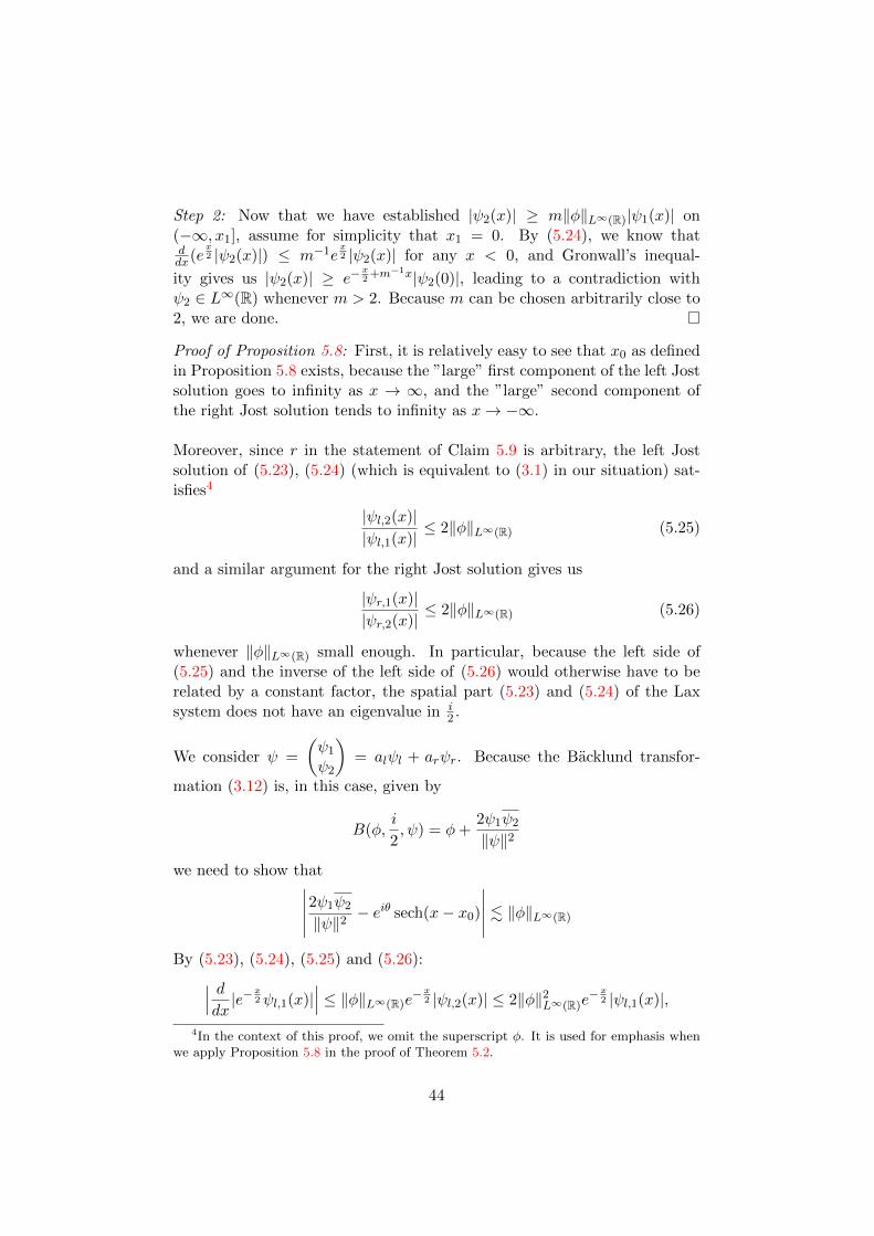
Proof of Proposition 5.8: First, it is relatively easy to see that x0 as definedin Proposition 5.8 exists, because the ”large” first component of the left Jostsolution goes to infinity as x → ∞, and the ”large” second component ofthe right Jost solution tends to infinity as x→ −∞.

Moreover, since r in the statement of Claim 5.9 is arbitrary, the left Jostsolution of (5.23), (5.24) (which is equivalent to (3.1) in our situation) sat-isfies4

|ψl,2(x)||ψl,1(x)|

≤ 2‖φ‖L∞(R) (5.25)

and a similar argument for the right Jost solution gives us

|ψr,1(x)||ψr,2(x)|

≤ 2‖φ‖L∞(R) (5.26)

whenever ‖φ‖L∞(R) small enough. In particular, because the left side of(5.25) and the inverse of the left side of (5.26) would otherwise have to berelated by a constant factor, the spatial part (5.23) and (5.24) of the Laxsystem does not have an eigenvalue in i

2 .

We consider ψ =

(ψ1

ψ2

)= alψl + arψr. Because the Backlund transfor-

mation (3.12) is, in this case, given by

B(φ,i

2, ψ) = φ+

2ψ1ψ2

‖ψ‖2

we need to show that∣∣∣∣∣2ψ1ψ2

‖ψ‖2− eiθ sech(x− x0)

∣∣∣∣∣ . ‖φ‖L∞(R)

By (5.23), (5.24), (5.25) and (5.26):∣∣∣ ddx|e−

x2ψl,1(x)|

∣∣∣ ≤ ‖φ‖L∞(R)e−x

2 |ψl,2(x)| ≤ 2‖φ‖2L∞(R)e−x

2 |ψl,1(x)|,

4In the context of this proof, we omit the superscript φ. It is used for emphasis whenwe apply Proposition 5.8 in the proof of Theorem 5.2.

44

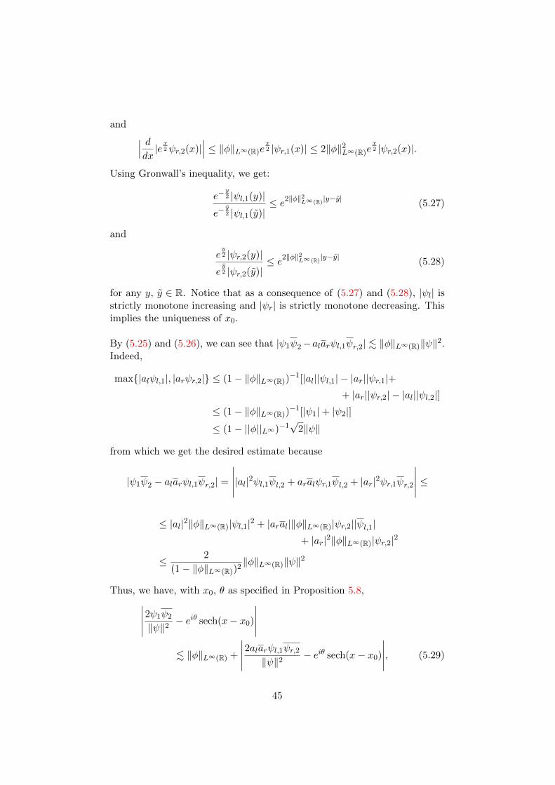
and ∣∣∣ ddx|ex2ψr,2(x)|

∣∣∣ ≤ ‖φ‖L∞(R)ex2 |ψr,1(x)| ≤ 2‖φ‖2L∞(R)e

x2 |ψr,2(x)|.

Using Gronwall’s inequality, we get:

e−y2 |ψl,1(y)|

e−y2 |ψl,1(y)|

≤ e2‖φ‖2L∞(R)|y−y| (5.27)

and

ey2 |ψr,2(y)|ey2 |ψr,2(y)|

≤ e2‖φ‖2L∞(R)|y−y| (5.28)

for any y, y ∈ R. Notice that as a consequence of (5.27) and (5.28), |ψl| isstrictly monotone increasing and |ψr| is strictly monotone decreasing. Thisimplies the uniqueness of x0.

By (5.25) and (5.26), we can see that |ψ1ψ2−alarψl,1ψr,2| . ‖φ‖L∞(R)‖ψ‖2.Indeed,

max|alψl,1|, |arψr,2| ≤ (1− ‖φ‖L∞(R))−1[|al||ψl,1| − |ar||ψr,1|+

+ |ar||ψr,2| − |al||ψl,2|]≤ (1− ‖φ‖L∞(R))

−1[|ψ1|+ |ψ2|]

≤ (1− ||φ||L∞)−1√

2‖ψ‖

from which we get the desired estimate because

|ψ1ψ2 − alarψl,1ψr,2| =

∣∣∣∣∣|al|2ψl,1ψl,2 + aralψr,1ψl,2 + |ar|2ψr,1ψr,2

∣∣∣∣∣ ≤≤ |al|2‖φ‖L∞(R)|ψl,1|2 + |aral|‖φ‖L∞(R)|ψr,2||ψl,1|

+ |ar|2‖φ‖L∞(R)|ψr,2|2

≤ 2

(1− ‖φ‖L∞(R))2‖φ‖L∞(R)‖ψ‖2

Thus, we have, with x0, θ as specified in Proposition 5.8,∣∣∣∣∣2ψ1ψ2

‖ψ‖2− eiθ sech(x− x0)

∣∣∣∣∣. ‖φ‖L∞(R) +

∣∣∣∣∣2alarψl,1ψr,2‖ψ‖2− eiθ sech(x− x0)

∣∣∣∣∣, (5.29)

45

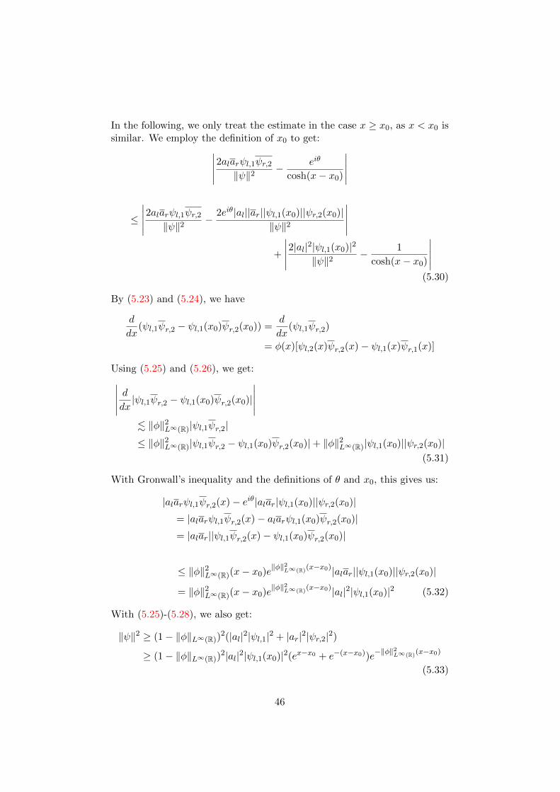
In the following, we only treat the estimate in the case x ≥ x0, as x < x0 issimilar. We employ the definition of x0 to get:∣∣∣∣∣2alarψl,1ψr,2‖ψ‖2

− eiθ

cosh(x− x0)

∣∣∣∣∣≤

∣∣∣∣∣2alarψl,1ψr,2‖ψ‖2−

2eiθ|al||ar||ψl,1(x0)||ψr,2(x0)|‖ψ‖2

∣∣∣∣∣+

∣∣∣∣∣2|al|2|ψl,1(x0)|2

‖ψ‖2− 1

cosh(x− x0)

∣∣∣∣∣(5.30)

By (5.23) and (5.24), we have

d

dx(ψl,1ψr,2 − ψl,1(x0)ψr,2(x0)) =

d

dx(ψl,1ψr,2)

= φ(x)[ψl,2(x)ψr,2(x)− ψl,1(x)ψr,1(x)]

Using (5.25) and (5.26), we get:∣∣∣∣∣ ddx |ψl,1ψr,2 − ψl,1(x0)ψr,2(x0)|

∣∣∣∣∣. ‖φ‖2L∞(R)|ψl,1ψr,2|

≤ ‖φ‖2L∞(R)|ψl,1ψr,2 − ψl,1(x0)ψr,2(x0)|+ ‖φ‖2L∞(R)|ψl,1(x0)||ψr,2(x0)|(5.31)

With Gronwall’s inequality and the definitions of θ and x0, this gives us:

|alarψl,1ψr,2(x)− eiθ|alar|ψl,1(x0)||ψr,2(x0)|= |alarψl,1ψr,2(x)− alarψl,1(x0)ψr,2(x0)|= |alar||ψl,1ψr,2(x)− ψl,1(x0)ψr,2(x0)|

≤ ‖φ‖2L∞(R)(x− x0)e‖φ‖2

L∞(R)(x−x0)|alar||ψl,1(x0)||ψr,2(x0)|

= ‖φ‖2L∞(R)(x− x0)e‖φ‖2

L∞(R)(x−x0)|al|2|ψl,1(x0)|2 (5.32)

With (5.25)-(5.28), we also get:

‖ψ‖2 ≥ (1− ‖φ‖L∞(R))2(|al|2|ψl,1|2 + |ar|2|ψr,2|2)

≥ (1− ‖φ‖L∞(R))2|al|2|ψl,1(x0)|2(ex−x0 + e−(x−x0))e

−‖φ‖2L∞(R)(x−x0)

(5.33)

46

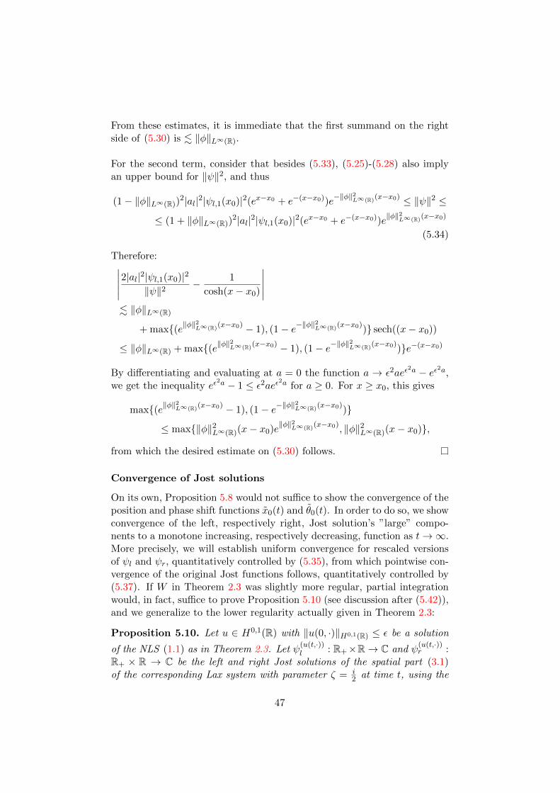
From these estimates, it is immediate that the first summand on the rightside of (5.30) is . ‖φ‖L∞(R).

For the second term, consider that besides (5.33), (5.25)-(5.28) also implyan upper bound for ‖ψ‖2, and thus

(1− ‖φ‖L∞(R))2|al|2|ψl,1(x0)|2(ex−x0 + e−(x−x0))e

−‖φ‖2L∞(R)(x−x0) ≤ ‖ψ‖2 ≤

≤ (1 + ‖φ‖L∞(R))2|al|2|ψl,1(x0)|2(ex−x0 + e−(x−x0))e

‖φ‖2L∞(R)(x−x0)

(5.34)

Therefore:∣∣∣∣∣2|al|2|ψl,1(x0)|2

‖ψ‖2− 1

cosh(x− x0)

∣∣∣∣∣. ‖φ‖L∞(R)

+ max(e‖φ‖2L∞(R)(x−x0) − 1), (1− e−‖φ‖

2L∞(R)(x−x0)

) sech((x− x0))

≤ ‖φ‖L∞(R) + max(e‖φ‖2L∞(R)(x−x0) − 1), (1− e−‖φ‖

2L∞(R)(x−x0)

)e−(x−x0)

By differentiating and evaluating at a = 0 the function a → ε2aeε2a − eε2a,

we get the inequality eε2a − 1 ≤ ε2aeε2a for a ≥ 0. For x ≥ x0, this gives

max(e‖φ‖2L∞(R)(x−x0) − 1), (1− e−‖φ‖

2L∞(R)(x−x0)

)

≤ max‖φ‖2L∞(R)(x− x0)e‖φ‖2

L∞(R)(x−x0), ‖φ‖2L∞(R)(x− x0),

from which the desired estimate on (5.30) follows.

Convergence of Jost solutions

On its own, Proposition 5.8 would not suffice to show the convergence of theposition and phase shift functions x0(t) and θ0(t). In order to do so, we showconvergence of the left, respectively right, Jost solution’s ”large” compo-nents to a monotone increasing, respectively decreasing, function as t→∞.More precisely, we will establish uniform convergence for rescaled versionsof ψl and ψr, quantitatively controlled by (5.35), from which pointwise con-vergence of the original Jost functions follows, quantitatively controlled by(5.37). If W in Theorem 2.3 was slightly more regular, partial integrationwould, in fact, suffice to prove Proposition 5.10 (see discussion after (5.42)),and we generalize to the lower regularity actually given in Theorem 2.3:

Proposition 5.10. Let u ∈ H0,1(R) with ‖u(0, ·)‖H0,1(R) ≤ ε be a solution

of the NLS (1.1) as in Theorem 2.3. Let ψ(u(t,·))l : R+×R→ C and ψ

(u(t,·))r :

R+ × R → C be the left and right Jost solutions of the spatial part (3.1)of the corresponding Lax system with parameter ζ = i

2 at time t, using the

47

same superscript notation as above. If we set ϕl(t, x) := e−x2ψ

(u(t,·))l (t, x)

and ϕ(t, x) := ϕl,1(t, tx), we have, for all sufficiently large t > 0,

|ϕ(t, x)− Pl(x)| . ε2 log(t)t−1+Cε2 , (5.35)

uniformly as t→∞, where

Pl(x) := exp

(−

x∫−∞

|W (y)|2

1− iydy

), (5.36)

with W ∈ H1−Cε2(R), C > 0 as in Theorem 2.3.In particular, this implies the pointwise convergence of ϕl,1(t, x)→ Pl(0) ast→∞ with an estimate

|ϕl,1(t, x)− Pl(0)| . ε2|x|t−1 + ε2 log(t)t−1+Cε2 (5.37)

Similar statements hold for the second component of the right Jost solutionψr(t, x) =: e−

x2ϕr(t, x), with ϕ replaced by φ(t, x) := ϕr,2(t, tx) and Pl by

Pr(x) := exp

(−∞∫x

|W (y)|2

1− iydy

)(5.38)

Proof. By Theorem 2.3, an asymptotic expression (2.9) for an NLS-potentialu(t, x) : R× R→ C with small ‖u(0, ·)‖H0,1(R) ≤ ε is given by

u(t, x) = t−12 ei

x2

2tW(xt

)ei log(t)|W (x

t)| + errx, (5.39)

where W ∈ H1−Cε2(R) and

errx ∈ εOL∞(R)((1 + t)−34

+Cε2) ∩OL2(R)((1 + t)−1+Cε2) (5.40)

For ease of notation we will modify ε to set C = 1.

We use the formula (4.11) from Remark 4.3. Then an easy change of vari-ables gives us, with w(t, x) = ei log(t)|W (x)|W (x),

ϕ(t, x) = 1−x∫

−∞

w(t, y)

y∫−∞

te−t(y−z)eit2

(y2−z2)w(t, z)ϕ(t, z)dzdy + e(t, x),

(5.41)

where we set e(t, x) := e1(t, x) + e2(t, x) + e3(t, x) with

e1(t, x) =

tx∫−∞

y∫−∞

t−12 ei

y2

2tW(yt

)ei log(t)|W ( y

t)|e−(y−z)errx(z)ϕ1(t, z)dzdy

48

and

e2(t, x) =

tx∫−∞

y∫−∞

errx(y)e−(y−z)t−12 e−i

z2

2tW(zt

)e−i log(t)|W ( z

t)|ϕ1(t, z)dzdy,

as well as

e3(x) =

tx∫−∞

y∫−∞

errx(y)e−(y−z)errx(z)ϕ1(t, z)dzdy

Young’s inequality and (5.40) immmediately give:

‖e1‖L∞(R) . ‖t−12W (t−1·)‖L2(R)‖e−t·‖L1(R+)‖errx‖L2(R)

= ‖W‖L2(R)‖errx‖L2(R) . ε2(1 + t)−1+ε2 ,

and similarly

‖e2‖L∞(R) . ε2(1 + t)−1+ε2 ,

as well as

‖e3‖L∞(R) ≤ ‖e−t·‖L1(R+)‖errx‖2L2(R) . ε2(1 + t)−2+2ε2

Hence, showing that (5.41) does, indeed, behave like (5.35) depends on themain term

x∫−∞

w(t, y)

y∫−∞

te−t(y−z)eit2

(y2−z2)w(t, z)ϕ(t, z)dzdy (5.42)

Applying a partial integration argument to (5.42) under the stronger as-sumption that W ∈ H1(R) with

‖W‖H1(R) . ε (5.43)

(and, for simplicity, also that |W | is differentiable everywhere) does, as we

claimed, suggest that limt→∞

ϕ(t, x) = exp(−

x∫−∞

|W (y)|21−iy dy

)uniformly at the

desired rate. Indeed, set the function

φ(t, z) :=ϕ(t, z)

1− iz(5.44)

Using e−t(y−z) = t−1∂ze−t(y−z), we get

x∫−∞

w(t, y)

y∫−∞

te−t(y−z)eit2

(y2−z2)w(t, z)φ(t, z)dzdy

=

x∫−∞

w(t, y)

y∫−∞

∂ze−t(y−z)e

it2

(y2−z2)w(t, z)φ(t, z)dzdy

49

=

x∫−∞

w(t, y)

[e−t(y−z)e

it2

(y2−z2)w(t, z)φ(t, z)

]yz=−∞

dy

+

x∫−∞

w(t, y)

y∫−∞

e−t(y−z)itzeit2

(y2−z2)w(t, z)φ(t, z)dzdy

+

x∫−∞

w(t, y)

y∫−∞

e−t(y−z)eit2

(y2−z2)∂zw(t, z)φ(t, z)dzdy

+

x∫−∞

w(t, y)

y∫−∞

e−t(y−z)eit2

(y2−z2)w(t, z)∂zφ(t, z)dzdy, (5.45)

and, using |w| = |W |,

w(t, y)

[e−t(y−z)e

it2

(y2−z2)w(t, z)φ(t, z)

]yz=−∞

=|W (y)|2

1− izϕ(t, y),

as well as (1 − iz)φ(t, z) = ϕ(t, z) by (5.44). Moreover, |∂zw(t, z)| .log(t)|W ′(z)| for sufficiently large t > 0, as well as |∂zφ(t, z)| . t|∂2ϕl,1(t, tz)|+|ϕl,1(t, tz)|. The boundedness of t|∂2ϕl,1(t, tz)| is a consequence of (4.12) andTheorem 2.3 (compare text after (5.56)), and the boundedness of |ϕl,1(t, z)|is, of course, known by Lemma 4.1. Using Young’s inequality and (5.43), wecan therefore bound the last two summands in (6.31) by ε2t−1 log(t), andthus

ϕ(t, x) = 1−x∫

−∞

|W (y)|2

1− iyϕ(t, y)dy +O(ε2 log(t)t−1) (5.46)

It seems natural that, for a slightly lower regularity than W ∈ H1(R), weget a loss in the rate of convergence of (5.46) as given in (5.35).

Thus, we know proceed with the general case of Theorem 2.3 that W ∈H1−ε2(R). We can now show (5.35) by proving that

x∫−∞

∣∣∣∣∣ |W (y)|2

1− iyϕ(t, y)−

− w(t, y)

y∫−∞

te−t(y−z)eit2

(y2−z2)w(t, z)ϕ(t, z)dz

∣∣∣∣∣dy . ε2 log(t)t−1+ε2

(5.47)

50

Before we show (5.47), we briefly establish that it does, indeed, imply (5.35).For, differentiating (5.41), we get

∂xϕ(t, x) = −|W (x)|2

1− ixϕ(t, x) + α(t, x), (5.48)

with

α(t, x) =|W (x)|2

1− ixϕ(t, x)−

− w(t, x)

x∫−∞

te−t(x−z)eit2

(x2−z2)w(t, z)ϕ(t, z)dzdy + ∂xe(t, x),

so if (5.47) holds, we havex∫−∞|α(t, y)|dy . ε log(t)t−1+ε2 . By variation of

constants, (5.48) has the general solution

C exp

(−

x∫−∞

|W (y)|2

1− iydy

)+

x∫−∞

exp

(−

x∫y

|W (y)|2

1− iydy

)α(t, y)dy

Because exp(−

x∫y

|W (y)|21−iy dy

)≤ exp(‖W‖2L2(R)) is bounded by a finite value,

the second summand is . ε log(t)t−1+ε2 . The definition of the left Jost so-lution ψl enforces C = 1, and hence we get (5.35).

To prove (5.47), notice that a partial integration ofx∫−∞

te−t(y−z)eit2

(y2−z2)dz

gives us

x∫−∞

t(

1− iz)e−t(y−z)e

it2

(y2−z2)dz = 1 (5.49)

Inserting (5.49) into the left side of (5.47) gives us that it is equal to

x∫−∞

∣∣∣∣∣|w(t, y)|2ϕ(t, y)

y∫−∞

1− iz1− iy

te−t(y−z)eit2

(y2−z2)dz

− w(t, y)

y∫−∞

te−t(y−z)eit2

(y2−z2)w(t, z)ϕ(t, z)dz

∣∣∣∣∣dy=

x∫−∞

∣∣∣∣∣|w(t, y)|2ϕ(t, y)

y∫−∞

1− iz1− iy

te−t(y−z)eit2

(y2−z2)dz−

51

− w(t, y)

y∫−∞

te−t(y−z)eit2

(y2−z2)w(t, z)ϕ(t, y)dz

+ w(t, y)

y∫−∞

te−t(y−z)eit2

(y2−z2)w(t, z)(ϕ(t, y)− ϕ(t, z))dz

∣∣∣∣∣dy,which is bounded by the following term:

x∫−∞

|w(t, y)|2|ϕ(t, y)|y∫

−∞

∣∣∣∣∣ i(y − z)1− iyte−t(y−z)e

it2

(y2−z2)

∣∣∣∣∣dzdy+

x∫−∞

|w(t, y)|y∫

−∞

∣∣∣∣∣1− iy1− iyte−t(y−z)e

it2

(y2−z2)(w(t, y)− w(t, z))ϕ(t, y)

∣∣∣∣∣dzdy+

x∫−∞

|w(t, y)|y∫

−∞

∣∣∣∣∣te−t(y−z)e it2 (y2−z2)w(t, z)(ϕ(t, y)− ϕ(t, z))

∣∣∣∣∣dzdy=: (I) + (II) + (III) (5.50)

Using (5.14), Young’s inequality and |w| = |W | (we suppress the explicitt-dependence of w in the following estimates):

(I) .

x∫−∞

|w(y)|2y∫

−∞

t(y − z)e−t(y−z)dzdy =1

t

x∫−∞

|w(y)|2∞∫

0

ze−zdzdy

.1

t‖w‖2L2 =

1

t‖W‖2L2 (5.51)

Moreover:

(II) ≤x∫

−∞

|w(y)||ϕ(t, y)|y∫

−∞

te−t(y−z)|w(y)− w(z)|dzdy

.

x∫−∞

|w(y)|∞∫

0

e−z∣∣∣w(y)− w

(y − z

t

)∣∣∣dzdy≤ ‖w‖L2(R)

∥∥∥∥∥∞∫

0

e−z∣∣∣w(y)− w

(y − z

t

)∣∣∣dz∥∥∥∥∥L2(R,dy)

(5.52)

Notice that the derivative of α → ei log(t)α has its absolute value boundedby log(t), so for y, y ∈ R, we have

|w(y)− w(y)| ≤ (1 + log(t))|W (y)−W (y)| (5.53)

52

by the definition of w. Furthermore, µ(z) = e−zdz, we get µ(R+) = 1, so byJensen’s inequality:∥∥∥∥∥∞∫

0

e−z∣∣∣W (y)−W

(y − z

t

)∣∣∣dz∥∥∥∥∥2

L2(dy)

≤∫R

∞∫0

e−z∣∣∣W (y)−W

(y − z

t

)∣∣∣2dzdy=

∞∫0

∫R

e−z∣∣∣W (y)−W

(y − z

t

)∣∣∣2dydz=

∞∫0

e−z∥∥∥W (y)−W

(y − z

t

)∥∥∥2

L2(dy)dz

≤∞∫

0

e−z(zt

)2(1−ε2)‖W‖2

H1−ε2 (R)dz

. t2(ε2−1)‖W‖2H1−ε2 (R)

, (5.54)

by a standard estimate on Hs-functions. Combined, (5.52), (5.53) and (5.54)give us that

|(II)| . log(t)t−1+ε2‖W‖H1−ε2 (R)

‖W‖L2(R) (5.55)

As for (III), by (4.12), we have

‖∂xϕl,1(t, x)‖L∞ . ‖u‖2L∞(R) (5.56)

And by (5.56), the definition of ϕ, and the asymptotic stability of Theorem2.3:

|ϕ(t, y)− ϕ(t, z)| ≤ t‖∂xϕl,1‖L∞(R)|y − z|. tε2t−1|y − z| = ε2|y − z|

Similarly to (I), this implies that we can control (III) by the estimate

|(III)| . 1

tε2‖w‖2L2(R) =

1

tε2‖W‖2L2(R) (5.57)

Together, (5.51), (5.55) and (5.57) give us (5.47), as desired. The pointwiseconvergence estimate (5.37) is now an easy consequence of (5.35), the factthat ϕ(t, 0) = ϕl,1(t, 0) ∀t > 0 by definition, and the bound ‖∂xϕl,1‖L∞(R) .ε2t−1 which holds by (5.56) and Theorem 2.3.

Remark 5.11. Like Lemma 5.6 and 5.7 and Proposition 5.8, Proposition5.10 is formulated specifically for ζ = i

2 here, but it is easy to see thatsimilar statements hold for any other ζ ∈ C with Im(ζ) > 0. In this case,it might be of particular interest to explicitly give the version of (5.36) and

53

(5.38) for general ζ in the upper halfspace. In that case, (5.49) is replaced

byy∫−∞

t(−2iζ − iz)eit2

(y2−z2)e2iζt(y−z)dz = 1, and hence we would have

Pl(x) = exp

( x∫−∞

|W (y)|2

2iζ + iydy

)

and

Pr(x) = exp

( ∞∫x

|W (y)|2

2iζ + iydy

),

for which similar estimates as in Proposition 5.10 hold, with constants inthe estimates depending on Im(ζ).

Proof of Theorem 5.2: Approximation of lower-regularity solu-tions and convergence of position and phase shift

We can now turn to the proof of our main theorem:

Proof of Theorem 5.2: We start with the assumption u ∈ C(R, H3(R)). Ourprevious considerations imply that, for sufficiently large t > 0,∥∥∥∥∥B(u(t, ·), i

2, ψ(t, x)

)− ei(t+θ(t)) sech(x− x0(t))

∥∥∥∥∥L∞(R)

. ε|t|−12 , (5.58)

for ψ as in (5.18), x0(t) the point where |clψ(u(t,x))l,1 (t, x)| = |crψ(u(t,x))

r,2 (t, x)|

and θ(t) the phase of clcrψ(u(t,x))l,1 (t, x0(t))ψ

(u(t,x))r,2 (t, x0(t)). Indeed, by Lemma

5.6 and 5.7 and the asymptotic stability result for the zero solution Theorem2.3, estimate (5.58) follows as a special case of Proposition 5.8, with φ = u,and

al = eit2 cl ar = e−

it2 cr (5.59)

for all large enough t ∈ R+. By well-posedness of the NLS,B(u(0, ·), i2 , ψ(0, x)) =u(0, ·) implies that we have B(u(t, ·), i2 , ψ(t, x)) = u(t, ·) ∀t > 0, so (5.2)holds for the original NLS solution u.

We now drop the assumption u0 ∈ H3(R)5. Let u0 ∈ H0,1(R) but /∈ H3(R)satisfy the assumptions of Theorem 5.2 and approximate it in L2(R) by a

5Alternatively to the following argument, it is also possible to proceed similarly as in[8] at the end of Sections 3.1.2 and 4 here.

54

sequence of H3(R)-functions u0n ∈ BH0,1(R)ε (sech(·)). By Theorem 5.1, at

any time t ≥ 0

un(t, ·)→ u(t, ·)

in the L2-sense, with un, u the NLS-solutions with initial data u0n and u0.

Let n ∈ N, the coefficients a(n)l (t) and a

(n)r (t) defined in the obvious manner

from (5.59) and the mapping B as in Lemma 4.7. Remember that by theremarks surrounding (5.5), we assume that the eigenvalue of the Lax system(3.1) with potential u0n is fixed at i

2 . Moreover, the proof of Lemma 4.7 es-tablished that B−1 is precisely given as the Backlund transformation arisingfrom the reiteration relation (3.14) - the same Backlund transformation weused to analyse the regular case. Our previous analysis for u0 ∈ H3(R) thusgives us that for

B(u0n) =( i

2, a(n)r (0)−1a

(n)l (0), u0n

)and un(t, ·) the unique NLS solution of Theorem 2.3 with un(0, ·) = u0n, wehave

B(un(t, ·)) =( i

2, a(n)r (t)−1a

(n)l (t), un(t, ·)

)(To understand the second component, compare (3.13) and the statementof Lemma 4.7.) Continuity of B now gives us that, as n→∞,

B(u0n) =( i

2, a(n)r (0)−1a

(n)l (0), u0n

)→ B(u0) =

( i2, αl(0), u0

)and, for t > 0,

B(un(t, ·)) =( i

2, a(n)r (t)−1a

(n)l (t), un(t, ·)

)→B(u(t, ·)) =

( i2, αl(t), u(t, ·)

)(5.60)

in C×C×L2(R). Recall here that a(n)r (t) 6= 0 for all t > 0 as a consequence

of Lemma 5.5, so all terms are well-defined.

Since the un are regular, Lemma 5.6 and 5.7 apply, i.e. a(n)l (t) = a

(n)l (0)e

i2t

and a(n)r (t) = a

(n)r (0)e−

i2t. In particular, (5.60) therefore implies

αl(t) = limn→∞

a(n)r (0)−1e

i2t · a(n)

l (0)ei2t = eita(n)

r (0)−1a(n)l (0) = eitαl(0)

Because

u(t, ·) = B−1( i

2, αl(t), u(t, ·)

)(t, ·),

55

we know, again by Lemma 4.7 and (3.13), that u is given as a Backlund

transformation u(t, ·) = B(u(t, ·), i2 , cle

i2tψ

(u(t,·))l + cre

− i2tψ

(u(t,·))r

)with cl =

αl(0) and cr = 1. Notice that by(5.60)

clcr∼ 1 (5.61)

still holds in the sense of Lemma 5.5. By Proposition 5.8, for sufficientlylarge t > 0:

‖u(t, ·)− ei(t+θ(t)) sech(·+ x0(t))‖L∞(R) . εt−12 ,

where the position and phase shift functions are still characterized by

|clψ(u(t,·))l (x0(t))| = |crψ(u(t,·))

r (x0(t))|

and

θ(t) = arg(clψ(u(t,·))l (x0(t))crψ

(u(t,·))r (x0(t)))

It now remains to prove the boundedness and the convergence (5.3) and(5.4) for the phase and position shift functions θ, x0. To do so, first considerthe position shift x0(t) for a fixed t > 0. The estimates (5.14) and (5.15)imply

(1− ε)ex2 ≤ |ψl,1(x)| ≤ (1 + ε)e

x2 (5.62)

and

(1− ε)e−x2 ≤ |ψr,2(x)| ≤ (1 + ε)e−

x2 (5.63)

With this and cl, cr as above, we get that |cl||ψl,1(x0(t))| = |cr||ψr,2(x0(t))|implies log

(|cr||cl|

1−ε1+ε

)≤ x0(t) ≤ log

(|cl||cr|

1+ε1−ε

). By (5.61), |cl||cr| ∼ 1, so |x0(t)| .

ε holds.

For θ, consider that for all x ∈ R, (5.14) and (5.15) give us:

|ψl,1(x)ψr,2(x)− 1| = |(ψl,1(x)− ex2 )ψr,2(x) + e

x2ψr,2(x)− 1|

≤ ‖(e−x2ψl,1(x)− 1)‖L∞(R)‖e

x2ψr,2(x)‖L∞(R)

+ ‖ex2ψr,2(x)− 1‖L∞(R)

≤ (1 + ε)ε+ ε

Moreover, Lemma 5.5 implies that arg(clcr) = arg(clc−1r ) . ε. Together,

this gives us arg(clcrψl,1(x)ψr,2(x)) . ε for all x ∈ R, and thus in particular,

|θ(t)| . ε.

56

For the convergence of position and phase x0(t), θ(t) as t→∞, we know byProposition 5.10 that there are constants Pl(0) and Pr(0) ∈ C such that

|ψl,1(t, x)− ex2Pl(0)| . ε2|x|e

x2 t−1 + ε2e

x2 log(t)t−1+Cε2 (5.64)

and

|ψr,2(t, x)− e−x2Pr(0)| . ε2|x|e−

x2 t−1 + ε2e−

x2 log(t)t−1+Cε2 (5.65)

We have, of course,

|Pl(0)− 1| . ε (5.66)

and

|Pr(0)− 1| . ε (5.67)

Define x0 by |cl||ex02 Pl(0)| = |cr||e−

x02 Pr(0)|. By Lemma 5.5, (5.66) and

(5.67), we have |x0| . ε. Setting y = x0(t) and y = x0 in (5.27) and (5.28),we obtain

|ψl,1(x0(t))||ψl,1(x0)|

≥ ex0(t)−x0

2−2ε2t−1|x0−x0(t)| (5.68)

and

|ψr,2(x0)||ψr,2(x0(t))|

≥ ex0(t)−x0

2−2ε2t−1|x0−x0(t)| (5.69)

Similarly:

|ψl,1(x0)||ψl,1(x0(t))|

≥ ex0−x0(t)

2−2ε2t−1|x0−x0(t)| (5.70)

and

|ψr,2(x0(t))||ψr,2(x0)|

≥ ex0−x0(t)

2−2ε2t−1|x0−x0(t)| (5.71)

Multiplying first the inequalities (5.68) and (5.69), letting t→∞, and thendoing the same for (5.70) and (5.71) gives, for sufficiently large t,

|x0(t)− x0| − 4ε2t−1|x0(t)− x0| .∣∣∣ log

( |ψl,1(x0)|ex02 |Pl(0)|

)− log

(e−x02 |Pr(0)||ψr,2(x0)|

)∣∣∣≤ log

(1 +|ψl,1(x0)− e

x02 Pl(0)|

ex02 |Pl(0)|

)+ log

(1 +|ψr,2(x0)− e−

x02 Pr(0)|

e−x02 |Pr(0)|

),

(5.72)

57

Because of (5.66), (5.67) and |x0| . ε, the right side of (5.72) is . |ψl,1(x0)−ex02 Pl(0)| + |ψr,2(x0) − e−

x02 Pr(0)|. By (5.64), (5.65) and, again, |x0| . ε,

this implies

|x0(t)− x0| . ε2|x0|ex0t−1 + ε2ex02 log(t)t−1+Cε2

. ε3eεt−1 + ε2eε2 log(t)t−1+Cε2

. ε2eε2 log(t)t−1+Cε2 ,

for ε small and t large enough, proving (5.3).

Finally, the estimates (5.14) and (5.15) already establish that ψl,1 and ψr,2are both Lipschitz continuous. Since we have x0(t)→ x0, it follows that

alarψl,1(x0(t))ψr,2(x0(t))− alarψl,1(x0)ψr,2(x0)→ 0,

where, as before, al = eit2 cl and ar = e−

it2 cr. This yields convergence of the

phase shift θ(t) to θ0 = arg(clcrPl(x0)Pr(x0)), with a rate of convergence atleast as good as x0(t), which shows (5.4).

58

Chapter 6

The mKdV Case

The spatial part (3.1) of the Lax system for mKdV is the same as for NLS,and as discussed in Chapter 2, we can use the Backlund transformation tomap the zero solution to solitons similarly to the NLS case. It is thus naturalto apply our methods from the previous chapter to the asymptotic stabilityof mKdV solitons. The well-posedness of mKdV in H1 follows, e.g., fromTheorem 3 in [7], which will take the place of Theorem 5.1 in the following.Similarly to Chapter 5, the solutions given by this result trivially have tocoincide with the solutions of Theorem 2.5 whenever its assumptions aresatisfied.

Theorem 6.1. Given a real-valued u0 ∈ H1,1(R) with ‖u0−sech(x)‖H1,1(R) =ε for a sufficiently small ε > 0, let u = u(t, x) : R+×R→ R be a real-valuedsolution of the focusing mKdV (1.3) in one dimension with u(0, ·) = u0(·).Then we have asymptotic stability in the sense that there is a constant λ ∈ Rsuch that for large enough t ∈ R+:

‖λu(λ3t, λ·)− sech(· − x0(t))‖L∞(R) . ε|t|−13 , (6.1)

where |λ − 1| . ε and |x0(t) − t| . ε for all t > 0. Moreover, the functionx0(t) satisfies lim

t→∞x0(t)− t = x0 ∈ R with

|x0(t)− t− x0| . ε2t−53 (6.2)

holding.

As with Theorem 5.2, while we only state Theorem 6.1 for the elementarysoliton to keep our argument simple, it generalizes to a similar statementfor the entire mKdV soliton group (2.8) via (2.7).

Proof. The Lax system for mKdV has the same spatial part as the NLSsystem, so Lemma 5.3 and Proposition 5.8 still apply. Furthermore, if thepotential is a solution of mKdV, the zero curvature condition (3.4) holds in

59

the mKdV case, too, i.e. ∂xB − ∂tA − [A,B] = 0, where A is the matrixfor the spatial part (3.1) and B for the temporal part (3.5) as given in(3.7). Thus, most arguments from the previous chapter can be repeated ina similar manner for the present proof, with the following modifications:

• The spatial part (3.1) with the real-valued potential u0 has a purelyimaginary eigenvalue ζ close to i

2 by Lemma 4.6. Because at t = 0 thescaling symmetry for mKdV (2.7) is the same as the scaling symmetryfor the NLS (2.2) at t = 0, we can fix the eigenvalue at ζ = i

2 byemploying the change of variables (5.5) with v = 0 (and, still, k =2 Im(ζ)).

• For the time evolution (5.21) for the left Jost solution at t = 0, whichis now given by

ψl(t, x) = e−σ2tψl(0, x) +

t∫0

e−σ(t−s)

2 (B(s, x) +σ

2)ψl(s, x)ds,

which, arguing as in Lemma 5.6 and 5.7, yields ψl(t, x) = e−t2ψ

(u(t,x))l (x)

for the time evolution of the left and ψr(t, x) = et2ψ

(u(t,x))r (x) for the

right Jost solution. This gives rise to the time evolution of mKdVsolitons (given as sech(x − t) for the elementary soliton) rather than

NLS solitons (given by eit2 sech(x)).

What remains to be shown is the convergence of the position function x0(t).Just as we used the asymptotic expression in Theorem 2.3 to this end forthe NLS system, we will use the asymptotics in Theorem 2.5 for mKdV:

By Lemma 5.8, x0 = x0(t) is characterized as the point where (with cland cr as in the previous chapter):

|cl|e−t2 |ψ(u(t))

l,1 (x0)| = |cr|et2 |ψ(u(t))

r,2 (x0)|, (6.3)

We can write1 (compare (4.15) from Remark 4.2 and (4.8), from which thesecond equation can be obtained in a similar way to (4.11) and (4.15)):

ex2ψ

(u(t))r,2 (x) =: ϕr(x) = 1−

∞∫x

∞∫y

u(y)e−(z−y)u(z)ϕr(z)dzdy

e−x2ψ

(u(t))l,1 (x) =: ϕl(x) = a

( i2

)+

∞∫x

y∫−∞

u(y)e−(y−z)u(z)ϕl(z)dzdy, (6.4)

1Notice that u = u because we are considering real-valued solutions.

60

where a denotes the inverse transmission coefficient. As in (5.62) and (5.63),ϕl(x) ∈ [(1 − ε)e

x2 , (1 + ε)e

x2 ] and ϕr(x) ∈ [(1 − ε)e−

x2 , (1 + ε)e−

x2 ], which

entails |x0(t)− t| . ε. Hence, for ε small enough, 12 x0 will be in the decaying

region Ω+0 of Theorem 2.5, assume e.g. x0 ≥ (1 − ε)t. By the same result,

‖t16 (t−

13x)u‖L2(Ω+

0 ) . ε, so by Young’s inequality

|ϕr(x0)− 1| =∞∫x0

∞∫y

u(y)e−(z−y)u(z)ϕr(z)dzdy . ‖u‖2L2(Ω+

0 )

. ε2(t−16 (t−

13 t)−1)2 = ε2t−

53

and (remember x0 > 0 by assumption):

|ϕl(x)− a( i

2

)| =

∣∣∣∣∣∞∫x0

y∫−∞

u(y)e−(y−z)u(z)ϕl(z)dzdy

∣∣∣∣∣ ≤≤

∣∣∣∣∣∞∫x0

y2∫

−∞

u(y)e−(y−z)u(z)ϕl(z)dzdy

∣∣∣∣∣+

∣∣∣∣∣∞∫x0

y∫y2

u(y)e−(y−z)u(z)ϕl(z)dzdy

∣∣∣∣∣. e−ct

∣∣∣∣∣∞∫x0

y2∫

−∞

u(y)e−12

(y−z)u(z)ϕl(z)dzdy

∣∣∣∣∣+ ‖u‖2L2(Ω+

0 )

. e−ct‖u‖2L2(R) + ε2t−53 ,

with c > 0. Thus, in (6.3) we equate

|cl|e−t2 e

x02

∣∣∣a( i2

)+O(ε2t−

53 )∣∣∣ = |cr|e

t2 e−

x02

∣∣∣1 +O(ε2t−53 )∣∣∣

From this, we get

x0(t)− t→ log

(|cr||cl|

a−1( i

2

))= log

(|cr||cl|

T( i

2

))=: x0,

and

|x0(t)− t− x0| . ε2t−53

as claimed in (6.2).

Unlike in the previous chapter, we did not establish any analogue ofProposition 5.10 in the above proof. This was not necessary, as the centerof the soliton is near +t and thus in the decaying region. Still, it remainsan interesting question if some kind of convergence of the right and left

61

Jost solution does hold as t → ∞. We will show so in the following. Asdiscussed in Chapter 1, this result might be useful in applying the methodsof this thesis to other special mKdV solutions that can be constructed viathe Backlund transformation:

Proposition 6.2. Let u = u(t, x) : R+ × R → C with ‖u(0, ·)‖H1,1(R) ≤ ε,ε > 0 small, be a real-valued solution of the mKdV (1.3) that satisfies

the assumptions of Theorem 2.5 and let ψ(u(t,x))l and ψ

(u(t,·))r be the cor-

responding right and left Jost solutions for the Lax system with parameterζ such that Im(ζ) > 0 (and the usual superscript notation). Let ϕl(t, x) :=

e−iζxψ(u(t,x))l (x), and writing the region Ω−0 defined in Theorem 2.5 as Ω−0 =

(−∞,−Kt13 ], K > 0, define

ϕ : R+ × [K12 t−

13 ,∞)→ C

ϕ(t, x) = ϕl,1(t,−tx2)

Then

‖ϕ(t, x)− Pl(x)‖L∞([K

12 t−

13 ,∞))

. εt−16 , (6.5)

where (with W as in Theorem 2.5) Pl : [K12 t−

13 ,∞)→ R is given by

Pl(x) = exp

(− 2 Im(ζ)π−1

∞∫x

|W (y)|2

4|ζ|2 + 4 Re(ζ)y + y2dy

),

as well as

|ϕl,1(t, x)− Pl(t−13 )| . εt−

16 (6.6)

for any x /∈ Ω−0 .

For ϕr(t, x) := eiζxψu(t,x)l (x), let

φ : R+ × [K12 t−

13 ,∞)→ C

φ(t, x) = ϕr,2(t,−tx2)

Then we have

‖φ(t, x)− Pr(x)‖L∞([K

12 t−

13 ,∞))

. εt−16 (6.7)

with Pr : [K12 t−

13 ,∞)→ R given by

Pr(x) = exp

(− 2 Im(ζ)π−1

x∫t−

13

|W (y)|2

4|ζ|2 + 4 Re(ζ)y + y2dy

),

62

as well as

|ϕr,2(t, x)− 1| . ε2t−13 (6.8)

for any x /∈ Ω−0 .

The basic structure of our proof of Proposition 6.2 is as follows:

• It is relatively easy to show (6.8) and that, provided (6.5) holds, (6.6)is also true. We will do so in Step 1 and Step 2 of the proof.

• In Step 3, we will show (6.5), which requires more work: Similar to theproof of Proposition 5.10, we will use the asymptotic expression on theoscillatory region of Theorem 2.5 to give the implicit representationof ϕ as the sum of a main term (6.12) and an error term which isunder control by Theorem 2.5. We will then further decompose (6.12)into four summands, which we will dub ”ab-part”, ”ab-part”, ”ab-part” and ”ab-part” (Step 3a)). As suggested by these names, thelatter two parts are given as complex conjugates of the former, so itsuffices to understand the behaviour of just the ”ab-part” and ”ab-part”. In Step 3b), we will treat the ”ab-part”, which is closest to theanalysis undertaken in Proposition 5.10: Partial integration under theassumption of slightly higher regularity suggests convergence to a time-independent integral as t → ∞, and we will estimate the differenceto this putative limit in the general case. In Step 3c), applying thesemethods to the ”ab-part” will give us that it behaves like an oscillatoryintegral (6.30), which, as we will show, converges to zero with anappropriate rate as t→∞. Step 3d) will summarize these results.

• Finally, we will sketch how a similar treatment of φ gives us (6.7) inStep 4.

Proof. For ease of notation, we will set ρ = 0 and use a ”toy version” of theregions introduced in Theorem 2.5, where we replace ”.” in the definition

of Ω+,0,−0 by ≤, e.g. Ω0

0 = x ∈ R : |x| ≤ t13 . For the same reason, we

restrict ourselves to ζ = i2 , the general case is a relatively straightforward

extension (compare Remark 5.11, (6.18) and (6.39)). Our final simplificationwill be to modify ε so that C = 1 in Theorem 2.5, i.e. W ∈ H1−ε2,1∩L∞(R)with ‖W‖

H1−ε2,1∩L∞(R). ε.

Step 1: Proof of (6.8)The estimate (6.8) is the simplest to show: We have

ϕr,2(t, x) := ex2ψr,2(t, x) = 1−

∞∫x

∞∫y

u(t, y)e−(z−y)u(t, z)ϕr,2(t, z)dzdy,

63

and we consider the case that [x,∞) ⊂ Ω00 ∪Ω+

0 . Now, by (2.11), (2.12) and(2.13), Theorem 2.5 entails that

‖u‖L2(Ω+0 ∪Ω0

0) . εt−16 + ‖Q(t−

13 ·)‖L2(Ω0

0)t− 1

3 + εt−518

+ 23Cε2

. εt−16 + ‖ε‖L2(Ω0

0)t− 1

3 + εt−518

+ 23Cε2

. εt−16 , (6.9)

where Q is the L∞-function on R specified in the same theorem, and, bydefinition, |Ω0

0| ∼ t13 . Young’s inequality yields:

|ϕr,2(t, x)− 1| ≤

∣∣∣∣∣∫

Ω+0 ∪Ω0

0

∞∫y

u(t, y)e−(z−y)u(t, z)ϕr,2(t, z)dzdy

∣∣∣∣∣. ‖u‖2

L2(Ω+0 ∪Ω0

0). ε2t−

13

for any x ∈ Ω00 ∪ Ω+

0 .

Step 2: (6.5) implies (6.6)Before we show the estimate (6.5), we will first establish that (6.6) followsfrom (6.5). We consider

ϕl,1(t, x) := e−x2ψl,1(t, x) = 1−

x∫−∞

y∫−∞

u(t, y)e−(y−z)u(t, z)ϕl,1(t, z)dzdy,

(6.10)

for x /∈ Ω−0 . We need to show that the contribution of Ω00 ∪ Ω+

0 × R to theabove integral goes to zero as t → ∞, with a rate of convergence that is. εt−

16 , from which (6.6) will follow. In particular, Ω−0 × Ω−0 is thus only

region to make a nonzero contribution to the limit of ϕl,1 as t→∞. Indeed,this is an easy implication of (6.9), which gives us∣∣∣∣∣

∫(−∞,x]∩(Ω0

0∪Ω+0 )

y∫−∞

u(t, y)e−(y−z)u(t, z)ϕl,1(t, z)dzdy

∣∣∣∣∣. ‖u‖L2(Ω0

0∪Ω+0 )‖u‖L2(R) . ε2t−

16

with Young’s inequality, and hence, for

ϕl,1(t, x) = 1−x∫

−∞

y∫−∞

u(t, y)e−(y−z)u(t, z)ϕl,1(t, z)dzdy

= ϕl,1(t,−t13 )−

x∫−t

13

y∫−∞

u(t, y)e−(y−z)u(t, z)ϕl,1(t, z)dzdy

64

=: ϕ(t, t−13 ) + I(x)

we have |I(x)| . ε2t−16 . If (6.5) holds, this implies (6.6). All other rates

of convergence we are going to establish in this proof are at least as fast asε2t−

16 .

Step 3: Proof of (6.5)To show (6.5), consider

ϕ(t, x) = ϕl,1(t,−tx2) = 1−∫

(−∞,−tx2]

∫(−∞,y]

u(y)e−(y−z)u(z)dzdy, (6.11)

for x ≥ t−13 (which is equivalent to (−∞,−tx2] ∈ Ω−0 ). On Ω−0 × Ω−0 , we

know by (2.14) that the potential is given by:

u(t, x) =π−12 t−

13 (t−

13 |x|)−

14 ·

· Re

(e

[iα(t,x)− 3i

4π|W (t−

12 |x|

12 )|2 log(t−

12 |x|

12 )

]W (t−

12 |x|

12 )

)+ E(x),

where α(t, x) = −23 t− 1

2 |x|32 + π

4 , W : R→ C with ‖W‖H1−ε,1∩L∞(R) . ε andthe error term E as in Theorem 2.5.

Step 3a): Decomposition of (6.11)We first estimate the contribution of all terms containing E to (6.11). By

Theorem 2.5, we have ‖E‖L2(Ω−0 ) . εt−16 , so Young’s inequality gives, for

x∗ ∈ Ω−0x∗∫−∞

y∫−∞

|E(y)|e−(y−z)|u(z)|dzdy +

x∗∫−∞

y∫−∞

|u(y)|e−(y−z)|E(z)|dzdy . ε2t−16 ,

as well asx∗∫−∞

y∫−∞

|E(y)|e−(y−z)|E(z)|dzdy . ε2t−13

Thus we are, similarly to the proof of Proposition 5.10, left to consider themain term given at the end of the following calculation:

π(1− ϕl,1(−tx2)) =

=

∞∫tx2

∞∫y

t−12 y−

14 z−

14 ey−zϕl,1(−z)·

· Re

[eiα(t,y)− 3i

4πlog(t−

12 y

32 )|W (t−

12 y

12 )|W (t−

12 y

12 )

]·

65

· Re

[eiα(t,z)− 3i

4πlog(t−

12 z

32 )|W (t−

12 z

12 )|W (t−

12 z

12 )

]dzdy

+O(ε2t−16 )

≈ 4

∞∫x

∞∫y

ty12 z

12 e−t(z

2−y2)ϕ(z) Re

[eiα(ty2)− 3i

4πlog(ty3)|W (y)|2W (y)

]·

· Re

[eiα(tz2)− 3i

4πlog(tz3)|W (z)|2W (z)

]dzdy,

(6.12)

using symmetry in the first equality and then a change of variables. Ascomplex numbers a and b generally satisfy

Re(ab) =1

4(ab+ ab+ ab+ ab), (6.13)

we can split the last integral (6.12) into four parts: An ”ab-part”

∞∫x

∞∫y

ty12 z

12 e−t(z

2−y2)ϕ(z)eiα(ty2)−iα(tz2)+ 3i4π

log(tz3)|W (z)|2− 3i4π

log(ty3)|W (y)|2 ·

·W (y)W (z)dzdy,(6.14)

an ”ab-part”

∞∫x

∞∫y

ty12 z

12 e−t(z

2−y2)ϕ(z)eiα(ty2)+iα(tz2)− 3i4π

log(ty3)|W (y)|2− 3i4π

log(tz3)|W (z)|2 ·

·W (y)W (z)dzdy,(6.15)

and an ”ab”- and ”ab”-part of (6.12) defined in the obvious way. It is, ofcourse, sufficient to understand the behaviour of (6.15) and (6.14), the othertwo summands just being the complex conjugates.

We will show that (6.14) (and hence its conjugate) goes to an integral of ϕmultiplied by a time-independent function, while (6.15) (and its conjugate)

goes to 0, all with the rate of convergence appropriately bounded by ε2t−16 .

Step 3b): The ”ab”-partFirst, we consider the ”ab”-part (6.14), which we will show goes to

∞∫x

|W (y)|2

2(1− iy)ϕ(t, y)dy (6.16)

66

To this end, we will proceed similarly to the NLS case in the last chapter.The difference of the ab-part from its putative limit (6.16) is bounded by

∞∫x

∣∣∣∣∣ |W (y)|2

2(1− iy)ϕ(y)− w(t, y)

∞∫y

ty12 z

12 e−t(z

2−y2)e23it(z3−y3)w(z)ϕ(z)dz

∣∣∣∣∣dy(6.17)

with w(t, x) := e−3i4π

log(tx3)|W (x)|2W (x). Now note that by partial integra-tion

∞∫y

ty12 z

12 e−t(z

2−y2)e23it(z3−y3)dz =

1

2(1− iy)+m(t, y) + n(t, y), (6.18)

where

m(t, y) = −1

4

∞∫y

y12 z−

32 e−t(z

2−y2)e23it(z3−y3)dz (6.19)

and

n(t, y) =

∞∫y

ity12 z

12 (z − y)e−t(z

2−y2)e23it(z3−y3)dz (6.20)

By definition, we have z ≥ y ≥ t−13 on the domain of integration, and

|z2 − y2| = |(z + y)(z − y)| ≥ 2t−13 |z − y|, which we can utilize to show that

the L∞([t−13 ,∞)) norm of m(t, ·) goes to zero as t→∞ with a rate of t−

13 .

For (6.20), consider that, if y ≥ t−13 ,

∞∫y

ty12 z

12 (z − y)e−t(z

2−y2)dz =

∞∫0

ty12 (z + y)

12 ze−t(z+2y)zdz

.

y∫0

tyze−2tyzdz +

∞∫y

tz2e−tz2dz

≤ t−1

∞∫0

ze−2zdz + te−12t13

∞∫y

z2e−12tz2dz,

(6.21)

so (6.20) is . t−1.

67

Because ‖W‖L2(R) . ε, inserting (6.18) into (6.17), these estimates give

us that the latter differs by O(ε2t−13 ) from

∞∫x

∣∣∣∣∣w(t, y)w(t, y)ϕ(y)

∞∫y

ty12 z

12 e−t(z

2−y2)e23it(z3−y3)dz

− w(t, y)

∞∫y

ty12 z

12 e−t(z

2−y2)e23it(z3−y3)w(t, z)ϕ(z)dz

∣∣∣∣∣dy,(6.22)

(Recall the definition of α here.) To get an appropriate bound for (6.22),notice that, for z > y > 0, by (4.12) and the chain rule (compare theestimate of term (III) from (5.50) in the last chapter),

|ϕ(t, y)− ϕ(t, z)| . ε2t13 z(z − y) (6.23)

Moreover, utilizing the derivatives of the functions z → eiC log(tz3) and|W (y)| → eiC log(tz3)|W (y)|2 , we get2:

|w(t, y)− w(t, z)| . log(t)∣∣∣|W (t, y)|2 − |W (t, z)|2

∣∣∣+ |W (y)−W (z)|

+ log(z)∣∣∣|W (t, y)|2 − |W (t, z)|2

∣∣∣+ ε2t13 (z − y), (6.24)

for large t (and, again, z > y > 0). By (6.23) and (6.24) (and, of course,L∞-boundedness of ϕ), (6.22) is smaller or equal to a constant times thesum of

∞∫x

|W (y)|∞∫y

log(t)ty12 z

12 e−t(z

2−y2)∣∣∣|W (y)|2 − |W (z)|2

∣∣∣dzdy (6.25)

and

∞∫x

|W (y)|∞∫y

ty12 z

12 e−t(z

2−y2)|W (y)−W (z)|dzdy (6.26)

and

∞∫x

|W (y)|∞∫y

log(z)ty12 z

12 e−t(z

2−y2)∣∣∣|W (y)|2 − |W (z)|2

∣∣∣dzdy (6.27)

2E.g., the last summand in (6.24) bounds the contribution of∣∣∣e 3i

4πlog(ty3)|W (y)|2W (y)−

e3i4π

log(tz3)|W (y)|2W (y)∣∣∣, since

∣∣∣∂z log(tz3)∣∣∣ =

∣∣∣ 3tz2tz3

∣∣∣ . t13 for z ≥ t−

13 .

68

and

ε2∞∫x

|W (y)|∞∫y

t43 y

12 z

12 (1 + z)(z − y)e−t(z

2−y2)dzdy (6.28)

Because W is both bounded and Holder continuous with exponent 1−ε22 ,

(6.25) can be estimated by

∞∫x

|W (y)|∞∫y

log(t)ty12 z

12 e−t(z

2−y2)|W (y)−W (z)|dzdy

. ε

∞∫x

|W (y)|∞∫y

log(t)ty12 z

12 e−t(z

2−y2)|y − z|1−ε2

2 dzdy,

from which we can proceed with a similar change of variables and calculationto (6.21):

= ε

∞∫x

|W (y)|∞∫

0

log(t)ty12 (z + y)

12 e−t(z+2y)zz

1−ε22 dzdy

. ε

∞∫x

|W (y)|y∫

0

log(t)tye−2tyzz1−ε2

2 dzdy+

+ ε

∞∫x

|W (y)|∞∫y

ty12 e−tz

2z

3−ε22 dzdy

= ε

∞∫x

|W (y)|ty2∫0

log(t)tye−2z( zty

) 1−ε22 1

tydzdy+

+ ε

∞∫x

|W (y)|∞∫y

log(t)ty12 e−tz

2z

3−ε22 dzdy

. ε log(t)t−1−ε2

2 ‖W‖L1(R)+

+ ε log(t)te−13tx2

∞∫x

y12 e−

13ty2 |W (y)|

∞∫y

e−13tz2z

3−ε22 dzdy

. ε log(t)(t−1−ε2

2 + te−13t13 )‖W‖L1(R) (6.29)

Notice that ‖W‖L1(R) . ‖W‖H0,1(R) . ε, so the right-hand side of (6.29) is

. ε2 log(t)t−1−ε2

2 . The integral (6.26) can be shown to be . ε2t−1−ε2

2 by a

69

similar, but simpler calculation. Now,

∞∫x

log(y)|W (y)|dy =

∞∫x

log(y)

y|y||W (y)|dy . ‖yW‖L2(R)

∥∥∥ log(y)

y

∥∥∥L2(R)

. ‖W‖H0,1(R),

so a minor modification of the argument for (6.25) gives us for (6.27):

∞∫x

|W (y)|∞∫y

log(z)ty12 z

12 e−t(z

2−y2)∣∣∣|W (y)|2 − |W (z)|2

∣∣∣dzdy. ε

∞∫x

|W (y)|∞∫

0

log(z + y)ty12 (z + y)

12 e−t(z+2y)zz

1−ε22 dzdy

. ε

∞∫x

|W (y)|y∫

0

log(y)tye−z( z

2ty

) 1−ε22 1

2tydzdy

+ ε

∞∫x

|W (y)|∞∫y

log(z)ty12 e−tz

2z

3−ε22 dzdy

. εt−1−ε2

2 ‖W‖H0,1(R) + εte−13t13 ‖W‖L1(R)

Finally, for (6.28),

ε2

∣∣∣∣∣∞∫x

|W (y)|∞∫y

t43 y

12 z

12 (1 + z)(z − y)e−t(z

2−y2)dzdy

∣∣∣∣∣ . ε2t−13 ,

also follows by spliting the integral and changing variables as in (6.21) and(6.29), for we get

∞∫y

t43 y

12 z

12 (1 + z)(z − y)e−t(z

2−y2)dz .

t−1y−1y∫0

t43 y(1 + y)

z

ty

1

tye−2zdz+

+

∞∫y

t43 z2(1 + z)e−tz

2dz,

which, for y ≥ t−13 , gives the desired estimate in the same way as before.

It follows that (6.22), and hence (6.17) does indeed go to zero with a rate

of convergence . ε2t−13 .

70

Step 3c): The ”ab”-partLet us now deal with the second summand indicated by (6.13), i.e. the”ab-part” (6.15):

∞∫x

∞∫y

ty12 z

12 e−t(z

2−y2)W (y)W (z)ϕ(z)

· ei(α(ty2)+α(tz2))− 3i4π

(log(ty3)|W (y)|2+log(tz3)|W (z)|2)dzdy

We are going to show that the absolute value of (6.15) is . ε2t−13

+2ε2 . Inorder to do so, we first show that for large t, this behaves like

∞∫x

−iϕ(y)

2(1 + iy)W (y)2e−

43ity3e−

3i2π

log(ty3)|W (y)|2dy. (6.30)

We use:

∞∫y

ty12 z

12 e−t(z

2−y2)e−23it(y3+z3)+iπ

2 dz =i

2

1

1 + iye−

43ity3 + r(t, y)

where our same considerations for (6.19), (6.20) apply to r. Thus, thedifference of (6.15) to (6.30) (w as in (6.17))∣∣∣∣∣

∞∫x

−iϕ(y)

2(1 + iy)W (y)2e−

43ity3e−

3i2π

log(ty3)|W (y)|2dy

−∞∫x

∞∫y

ty12 z

12 e−t(z

2−y2)w(y)w(z)ϕ(z)e23it(y3+z3)dzdy

∣∣∣∣∣is, except for an error of O(ε2t−

13 ), given by∣∣∣∣∣

∞∫x

∞∫y

ty12 z

12 e−t(z

2−y2)e23it(y3+z3)w(t, y)[ϕ(y)w(t, y)− ϕ(z)w(t, z)]dzdy

∣∣∣∣∣This can be shown to be . ε2t−

13 by the same estimates we used for (6.22).

(Notice that these estimates only used the absolute values of the integrands,

and |e23it(y3+z3)| = |e

23it(y3−z3)| = 1.)

Now, we want to show that (6.30) goes to 0 with a sufficiently fast rateas t→∞. Let us first work with the stronger assumption W ∈ H1(R) and

71

‖W‖H1 . ε, so that partial integration yields:

∞∫x

−iϕ(y)W (y)2

2(1 + iy)e−

43ity3e−

3i2π

log(ty3)|W (y)|2dy =

=

∞∫x

ϕ(y)W (y)2

2(1 + iy)

∂ye− 4

3ity3

4ty2e−

3i2π

log(ty3)|W (y)|2dy

=ϕ(x)W (x)2

2(1 + ix)

e−43itx3

4tx2e−

3i2π

log(tx3)|W (x)|2

−∞∫x

∂yϕ(y)W (y)2

2(1 + iy)

e−43ity3

4ty2e−

3i2π

log(ty3)|W (y)|2dy

−∞∫x

ϕ(y)W (y)2∂y

[1

8y2(1 + iy)

]e−

43ity3

te−

3i2π

log(ty3)|W (y)|2dy

−∞∫x

2W (y)∂yW (y)ϕ(y)

2(1 + iy)

e−43ity3

4ty2e−

3i2π

log(ty3)|W (y)|2dy

+

∞∫x

ϕ(y)W (y)2

2(1 + iy)

e−43ity3

4ty2

3i

2π

3

y|W (y)|2e−

3i2π

log(ty3)|W (y)|2dy

+

∞∫x

ϕ(y)W (y)2

2(1 + iy)

e−43ity3

4ty2|W (y)|2 3i

πlog(ty3)·

· Re

[W (y)∂yW (y)

]e−

3i2π

log(ty3)|W (y)|2dy (6.31)

Because x ≥ t−13 , ‖W‖L2∩L∞(R) ≤ ε, ‖∂yW (y)‖L2(R) and (as can be seen

from (6.23)) |∂yϕ(y)| . ε|y|t−13 , each of these summands can be bounded

by a term that is . ε2t−13 .

Finally, we use an approximation argument to prove that (6.30) is . ε2t−13

+2ε2

in the general case of Theorem 2.5, i.e. just ‖W‖H1−ε2,1∩L∞(R)

. ε. Re-

call that Hs(Rn) is an algebra with respect to multiplication of functionswhenever s ≥ n

2 , and ‖fg‖Hs . ‖f‖Hs‖g‖Hs in that case. Therefore,

W ∈ H1−ε2(R) implies V := |W |2 ∈ H1−ε(R) for ε small enough, and‖V ‖

H1−ε2 (R). ‖W‖2

H1−ε2 (R). Pick a smooth cutoff function φ : R→ R with

72

Fourier transformation φ(ξ) = 1 for |ξ| ≤ 1 and φ(ξ) = 0 for |ξ| ≥ 2. In thatcase, with δ = δ(t) > 0 to be chosen later:∥∥∥F−1

[φ( ·δ

)V]∥∥∥2

H1∼∫R

(1 + |ξ|2)∣∣∣φ(ξ

δ

)∣∣∣2|V (ξ)|2dξ

. (1 + |δ|2)ε2‖V ‖2

H1−ε2 (R)(6.32)

and ∥∥∥F−1[(

1− φ( ·δ

))V]∥∥∥2

H34∼∫R

(1 + |ξ|2)34

∣∣∣1− φ(ξδ

)∣∣∣2|V (ξ)|2dξ

≤ (1 + |δ|2)−14

+ε2‖V ‖2H1−ε2 (R)

(6.33)

Thus, we can write |W (y)|2 = G(y)+H(y) withG ∈ C∞0 (R) and itsH1-norm

controlled by (6.32), while H’s H34 -norm and thus its L∞-norm is bounded

by (6.33). We can construct a similar decomposition W 2(y) = M(y)+N(y).We obtain:∞∫x

−iϕ(y)

2(1 + iy)W (y)2e−

43ity3e−

3i2π

log(ty3)|W (y)|2dy

=

∞∫x

−iϕ(y)

2(1 + iy)M(y)e−

43ity3e−

3i2π

log(ty3)|W (y)|2dy

+

∞∫x

−iϕ(y)

2(1 + iy)N(y)e−

43ity3e−

3i2π

log(ty3)|W (y)|2dy

=

∞∫x

−iϕ(y)

2(1 + iy)M(y)e−

43ity3e−

3i2π

log(ty3)[G(y)+H(y)]dy

+

∞∫x

−iϕ(y)

2(1 + iy)N(y)e−

43ity3e−

3i2π

log(ty3)|W (y)|2dy

=

∞∫x

−iϕ(y)

2(1 + iy)M(y)e−

43ity3e−

3i2π

log(ty3)G(y)dy

+

∞∫x

−iϕ(y)

2(1 + iy)M(y)e−

43ity3e−

3i2π

log(ty3)G(y)(e−3i2π

log(ty3)H(y) − 1)dy

+

∞∫x

−iϕ(y)

2(1 + iy)N(y)e−

43ity3e−

3i2π

log(ty3)|W (y)|2dy

=: (A) + (B) + (C) (6.34)

73

The obvious modification of the partial integration (6.31) for more regularW , combined with (6.32), gives us for the first term:

|(A)| . ‖W‖2H1−ε2 (R)

(1 + δ(t)2)ε2

2 · t−13 , (6.35)

while the analogue to (6.33) for the function N shows

|(C)| . ‖W‖2H1−ε2 (R)

(1 + δ(t)2)−18

+ ε2

2 (6.36)

For the second term (B), we have∣∣∣∣∣∞∫x

−iϕ(y)

2(1 + iy)M(y)e−

43ity3e−

3i2π

log(ty3)G(y)(e−3i2π

log(ty3)H(y) − 1)dy

∣∣∣∣∣ .

.

∞∫x

1

|1 + iy||M(y)|| log(ty3)H(y)|dy

. log(t)(1 + |δ|2)−18

+ ε2

2

∞∫x

1

|1 + iy||M(y)|dy

+ (1 + |δ|2)−18

+ ε2

2

∞∫x

log(y)

|1 + iy||M(y)|dy

(6.37)

Because M ∈ L2(R) with ‖M‖L2(R) . (1 + δ(t)2)ε2

2 ‖W‖2H1−ε2 (R)

(similar to

(6.32)), choosing

δ(t) ∼ t2 (6.38)

with appropriate α > 18−ε2 therefore gives us:

|(B)| . ‖W‖2H1−ε2 (R)

log(t)t−12

+4ε2 ,

while (6.35) and (6.36) become:

|(A)| . ‖W‖2H1−ε2 (R)

t−13

+2ε2

and

|(C)| . ‖W‖2H1−ε2 (R)

t−12

+2ε2

74

which, if ε is small enough, shows that (6.34) is . ε2t−13

+2ε.

Step 3d): ResultWe can now apply our results for (6.14) and (6.15) to their complex conju-gates ”ab”-part and ”ab”-part of (6.13). Putting all of this together givesus, with (6.16) and

1

2(1 + iy)+

1

2(1− iy)=

1

1 + y2(6.39)

that

ϕ(t, x) = 1−∞∫

maxt−13 ,x

|W (y)|2

1 + y2ϕ(t, y)dy +R(t, x)

where |R(t, x)| . ε2t−16 . Arguing as we did in the previous chapter after

(5.48), (6.5) follows.

Step 4: Sketch of proof of (6.7)For the proof of (6.7), we can repeat many arguments from the proof of(6.5). For the right Jost solution, we consider

φ(t, x) = ϕ(r)2 (t,−tx2) = 1 +

∞∫−tx2

∞∫y

u(t, y)e−(z−y)u(t, z)ϕ(r)2 (t, z)dzdy

for x ∈ [t−13 ,∞) (and hence −tx2 ∈ Ω−0 by our setting C = 1). We can

control∞∫

−t13

∞∫y

u(t, y)e−(z−y)u(t, z)ϕr,2(t, z)dzdy

and∞∫

−tx2

∞∫−t

13

u(t, y)e−(z−y)u(t, z)ϕr,2(t, z)dzdy

by ε2t−16 because of (6.9) and Young’s inequality. Similarly as in (6.12), we

obtain

φ(t, x) = O(ε2t−16 )+

+ 4π−1

x∫t−

13

y∫t−

13

ty12 z

12 e−t(z

2−y2)ϕ(z) Re

[eiα(ty2)− 3i

4πlog(ty3)|W (y)|2W (y)

]·

75

· Re

[eiα(tz2)− 3i

4πlog(tz3)|W (z)|2W (z)

]dzdy,

(6.40)

with α as in Theorem 2.5. We can, again, use (6.13) to decompose the lastintegral into four summands. The analogue of the ”ab”-part (6.14) is

x∫t−

13

y∫t−

13

ty12 z

12 et(z

2−y2)e23it(z3−y3)w(t, y)w(z)ϕ(z)dzdy (6.41)

with w(t, x) = e−3i4π

log(tx3)|W (x)|2W (x), as in Step 3. Partial integrationgives

(1 + iy)

y∫t−

13

ty12 z

12 et(z

2−y2)e23it(z3−y3)dz

=1

2− 1

2y

12 t

16 et(t

− 23−y2)e

23it(t−1−y3) + m(t, y) + n(t, y) (6.42)

with

m(t, y) =1

4

y∫t−

13

y12 z−

32 et(z

2−y2)e23it(z3−y3)dz (6.43)

and

n(t, y) =

y∫t−

13

ity12 z

12 (y − z)et(z2−y2)e

23it(z3−y3)dz, (6.44)

Equation (6.42) plays the same role here as (6.18) did for the left Jostsolution, and (6.43) and (6.44) can be bounded in the same way as (6.19)and (6.20). Moreover

x∫t−

13

∣∣∣12y

12 t

16 et(t

− 23−y2)e

23it(t−1−y3)W (y)2

∣∣∣dy ≤ 1

2

x∫t−

13

|y|12 t

16 et

23 (t−

13−y)|W (y)|2dy

≤ εt16 ‖e−t

23 ·‖L1(R+)‖W (y)‖H0,1(R)

≤ ε2t−12

So we get, similarly to our treatment of (6.17)

x∫t−

13

∣∣∣∣∣ |W (y)|2

2(1 + iy)ϕ(y)− w(t, y)

y∫t−

13

ty12 z

12 et(z

2−y2)e23it(z3−y3)w(z)ϕ(z)dz

∣∣∣∣∣dy

76

=

x∫t−

13

∣∣∣∣∣w(t, y)w(t, y)ϕ(y)

y∫t−

13

ty12 z

12 et(z

2−y2)e23it(z3−y3)dz

− w(t, y)

y∫t−

13

ty12 z

12 et(z

2−y2)e23it(z3−y3)w(t, z)ϕ(z)dz

∣∣∣∣∣dy+O(ε2t−

13 ),

on which similar estimates as for (6.22) can be used to show that (6.41)converges at the desired rate. E.g., in place of (6.25), we get

x∫t−

13

|W (y)|y∫

t−13

log(t)ty12 z

12 e−t(z

2−y2)∣∣∣|W (y)|2 − |W (z)|2

∣∣∣dzdy.

x∫t−

13

|W (y)|y∫

t−13

log(t)ty12 z

12 e−t(z

2−y2)|y − z|1−ε2 dzdy

=

x∫t−

13

|W (y)|y−t−

13∫

0

t log(t)y12 (y − z)

12 e−t(2y−z)zz

1−ε2 dzdy

≤x∫

t−13

|W (y)|y−t−

13∫

0

t log(t)ye−tyzz1−ε2 dzdy,

and this is . ε2 log(t)t−1−ε2 by the calculation (6.29). Terms (6.26), (6.27)

and (6.28) can be bounded in a very similar manner. The analogue of the”ab-part” can also be treated similarly as we did (6.15) in Step 3b). Inparticular, notice that in place of (6.30), we get

x∫t−

13

−iϕ(y)

2(1 + iy)W (y)2e−

43ity3e−

3i2π

log(ty3)|W (y)|2dy

=

∞∫t−

13

−iϕ(y)

2(1 + iy)W (y)2e−

43ity3e−

3i2π

log(ty3)|W (y)|2dy−

−∞∫x

−iϕ(y)

2(1 + iy)W (y)2e−

43ity3e−

3i2π

log(ty3)|W (y)|2dy,

so our estimates for (6.30) also cover this case.

77

Bibliography

[1] Ablowitz, Mark J., et al. ”The inverse scattering transform-Fourieranalysis for nonlinear problems.” Studies in Applied Mathematics 53.4(1974): 249-315.

[2] de Bouard, Anne, Nakao Hayashi, and Jean-Claude Saut. ”Global ex-istence of small solutions to a relativistic nonlinear Schrodinger equa-tion.” Communications in Mathematical Physics 189.1 (1997): 73-105.

[3] Cascaval, Radu C., et al. ”Spectral analysis of Darboux transformationsfor the focusing NLS hierarchy.” Journal D’Analyse Mathematique 93.1(2004): 139-197.

[4] Cazenave, Thierry. An introduction to nonlinear Schrodinger equations.Vol. 22. Universidade Federal do Rio de Janeiro, Centro de CienciasMatematicas e da Natureza, Instituto de Matematica, 1989.

[5] Chen, Gong, and Jiaqi Liu. ”Long-time asymptotics of the mod-ified KdV equation in weighted Sobolev spaces.” arXiv preprintarXiv:1903.03855 (2019).

[6] Chen, Gong, and Jiaqi Liu. ”Soliton resolution for the modified KdVequation.” arXiv preprint arXiv:1907.07115 (2019).

[7] Colliander, James, et al. ”Sharp global well-posedness for KdV andmodified KdV on R and T.” Journal of the American MathematicalSociety 16.3 (2003): 705-749.

[8] Cuccagna, Scipio, and Dmitry E. Pelinovsky. ”The asymptotic stabilityof solitons in the cubic NLS equation on the line.” Applicable Analysis93.4 (2014): 791-822.

[9] Deimling, Klaus. Nonlinear functional analysis. Courier Corporation,2010.

[10] Dull, Wolf-Patrick, Guido Schneider, and C. Eugene Wayne. ”Justifica-tion of the Nonlinear Schrodinger equation for the evolution of gravitydriven 2D surface water waves in a canal of finite depth.” Archive forRational Mechanics and Analysis 220.2 (2016): 543-602.

78

[11] Faddeev, Ludwig, and Leon Takhtajan. Hamiltonian methods in thetheory of solitons. Springer Science & Business Media, 2007.

[12] Harrop-Griffiths, Benjamin. ”Long time behavior of solutions to themKdV.” Communications in Partial Differential Equations 41.2 (2016):282-317.

[13] Hayashi, Nakao, and Pavel I. Naumkin. ”Asymptotics for large time ofsolutions to the nonlinear Schrodinger and Hartree equations.” Ameri-can Journal of Mathematics 120.2 (1998): 369-389.

[14] Hayashi, Nakao, and Pavel I. Naumkin. ”Large time behavior of solu-tions for the modified Korteweg-de Vries equation.” International Math-ematics Research Notices 1999.8 (1999): 395-418.

[15] Hayashi, Nakao, and Pavel Naumkin. ”On the modified Korteweg–deVries equation.” Mathematical Physics, Analysis and Geometry 4.3(2001): 197-227.

[16] Ifrim, Mihaela, and Daniel Tataru. ”Global bounds for the cubic nonlin-ear Schrodinger equation (NLS) in one space dimension.” Nonlinearity28.8 (2015): 2661.

[17] Kibler, Bertrand, et al. ”The Peregrine soliton in nonlinear fibre optics.”Nature Physics 6.10 (2010): 790.

[18] Koch, Herbert, and Daniel Tataru. ”Conserved energies for the cubicnonlinear Schrodinger equation in one dimension.” Duke MathematicalJournal 167.17 (2018): 3207-3313.

[19] Lamb Jr, George L. ”Elements of soliton theory.” New York, Wiley-Interscience, 1980.

[20] Linares, Felipe, and Gustavo Ponce. Introduction to nonlinear disper-sive equations. Springer, 2014.

[21] Miller, Peter D. ”Lecture 11: The Inverse-Scattering Trans-form for the Focusing Nonlinear Schrodinger Equation”, Uni-versity of Arizona. Captured by Internet Archive in 2016:https://web.archive.org/web/20160221135849/http://math.

arizona.edu/~mcl/Miller/MillerLecture11.pdf

[22] Mizumachi, Tetsu, and Dmitry Pelinovsky. ”Backlund transformationand L2-stability of NLS solitons.” International Mathematics ResearchNotices 2012.9 (2012): 2034-2067.

[23] Parlakgorur, Tugce, and Oktay K. Pashaev. ”Nonlinear Cauchy-Riemann Equations and Liouville Equation For Conformal Metrics.”arXiv preprint arXiv:1706.10201 (2017).

79

[24] Tao, Terence. ”Why are solitons stable?.” Bulletin of the AmericanMathematical Society 46.1 (2009): 1-33.

[25] Tsutsumi, Yoshio. ”L2-Solutions for Nonlinear Schrodinger Equationsand Nonlinear Groups.” Funkcialaj Ekvacioj 30 (1987): 115-125.

80