Embed Size (px)
Citation preview

i
Mapping Habitat and Potential Distributions of Invasive
Plant Species on USFWS National Wildlife Refuges
Paul Evangelista1, Nicholas Young
1, Lane Carter
2, Catherine Jarnevich
3,
Amy Birtwistle2, and Kelli Groy
2
Alligator Weed (Alternanthera philoxeroides )
Natural Resource Ecology Laboratory1 and ColoradoView
2
Colorado State University
U.S. Geological Survey
Fort Collins Science Center3
October 1, 2012

ii
TABLE OF CONTENTS
LIST OF TABLES ..................................................................................................................................... iii
LIST OF FIGURES ................................................................................................................................... iv
LIST OF APPENDICES ............................................................................................................................. v
INTRODUCTION ...................................................................................................................................... 1
GOALS AND OBJECTIVES ..................................................................................................................... 3
METHODS ................................................................................................................................................. 3
Study Sites and Priority Species .............................................................................................................. 3
Model Selection and Comparisons .......................................................................................................... 4
Predictor Variables ................................................................................................................................. 5
Modeling ................................................................................................................................................. 6
RESULTS ................................................................................................................................................... 7
Model Comparisons ................................................................................................................................ 7
Final Models: Alligator River NWR and South Atlantic LCC ................................................................. 9
Final Models: Quivira NWR and Great Plains LCC ............................................................................. 12
Final Models: Silvio O. Conte NWR and North Atlantic LCC .............................................................. 15
Final Models: San Diego NWR and California LCC ............................................................................ 18
DISCUSSION ........................................................................................................................................... 21
CONCLUSION......................................................................................................................................... 22
ACKNOWLEDGEMENTS ...................................................................................................................... 23
REFERENCES ......................................................................................................................................... 24
APPENDICES ............................................................................................................................................. I

iii
LIST OF TABLES
Table 1. List and description of BioClim seasonal climatic indices used for LCC modeling. For more
detailed information, see Hijmans, 2006. .................................................................................................... 6
Table 2. Table of comparison AUC values reported by all models tested at both the refuge scale and LCC
scale for each invasive species. The chosen Maxent modeling method values include Training and Test
AUC’s. ........................................................................................................................................................ 7
Table 3. The top three environmental predictors and their percent contribution for alligator weed in
Alligator River NWR. ................................................................................................................................. 9
Table 4. The top five environmental predictors and their percent contribution for alligator weed in South
Atlantic LCC............................................................................................................................................. 10
Table 5. Top three environmental predictors and their percent contribution for Phragmites spp. in
Alligator River NWR. ............................................................................................................................... 11
Table 6. Top five environmental predictors and their percent contribution for Phragmites spp. in South
Atlantic LCC............................................................................................................................................. 11
Table 7. Top three environmental predictors and their percent contribution for tamarisk in Quivira NWR.
.................................................................................................................................................................. 12
Table 8. Top five environmental predictors and their percent contribution for tamarisk in Great Plains
LCC. ......................................................................................................................................................... 13
Table 9. Top three environmental predictors and their percent contribution for Phragmites spp. in Quivira
NWR. ........................................................................................................................................................ 14
Table 10. The top five environmental predictors and their percent contribution for Phragmites spp. in
Great Plains LCC. ..................................................................................................................................... 14
Table 11. The top three environmental predictors and their percent contribution for garlic mustard in
Silvio O. Conte NWR. .............................................................................................................................. 15
Table 12. The top five environmental predictors and their percent contribution for garlic mustard in North
Atlantic LCC............................................................................................................................................. 16
Table 13. Top three environmental predictors and their percent contribution for Japanese stiltgrass in
Silvio O. Conte NWR. .............................................................................................................................. 17
Table 14. Top five environmental predictors and their percent contribution for Japanese stiltgrass in the
North Atlantic LCC. ................................................................................................................................. 17
Table 15. Top three environmental predictors and their percent contribution for false brome in San Diego
NWR. ........................................................................................................................................................ 18
Table 16. Top five environmental predictors and their percent contribution for false brome in the
California LCC. ........................................................................................................................................ 19
Table 17. Top three environmental predictors and their percent contribution for Sahara mustard in San
Diego NWR. ............................................................................................................................................. 20

iv
Table 18. Top five environmental predictors and their percent contribution for Sahara mustard in the
California LCC. ........................................................................................................................................ 20
LIST OF FIGURES
Figure 1. Diagrammatic representation of ecological niche modeling components for modeling species
distributions. Bottom part of the figure shows potential habitat distribution map for invasive plant
dalmation toadflax (Linaria dalmatica) in Colorado, USA (adapted from Franklin, 2009). ....................... 2
Figure 2. Model results for alligator weed at Alligator River NWR. The models tested were (A) Boosted
Regression Tree, (B) Multivariate Adaptive Regression Splines, (C) Maxent and (D) General Linear
Model. ......................................................................................................................................................... 8
Figure 3. Model results for tamarisk at Quivira NWR. The models tested were (A) Boosted Regression
Tree, (B) Multivariate Adaptive Regression Splines, (C) Maxent and (D) General Linear Model.............. 9
Figure 4. Predicted distribution of alligator weed in Alligator River NWR (left) and the South Atlantic
LCC (right) using the Maxent model. ....................................................................................................... 10
Figure 5. Predicted distribution of Phragmites spp. in Alligator River NWR (left) and the South Atlantic
LCC (right) using the Maxent model. ....................................................................................................... 12
Figure 6. Predicted distribution of tamarisk in Quivira NWR (left) and the Great Plains LCC (right) using
the Maxent model ..................................................................................................................................... 13
Figure 7. Predicted distribution of Phragmites spp. in Quivira NWR (left) and the Great Plains LCC
(right) using the Maxent model. ................................................................................................................ 15
Figure 8. Predicted distribution of garlic mustard in North Atlantic LCC (right) using the Maxent model.
.................................................................................................................................................................. 16
Figure 9. Predicted distribution of Japanese stiltgrass in North Atlantic LCC (right) using the Maxent
model. ....................................................................................................................................................... 18
Figure 10. Predicted distribution of false brome in California LCC (right) using the Maxent model. ...... 19
Figure 11. Predicted distribution of Sahara mustard in California LCC (right) using the Maxent model.. 21

v
LIST OF APPENDICES
Appendix 1. Predictor variables used to generate models at each refuge. The Source of the predictor
variable Land Cover Type varied from GAP (Quivira), DARE (Alligator River), and Landfire(Silvio O.
Conte), Vegetation 1995 (San Diego) depending on the refuge. .................................................................. I
Appendix 2. Model results for Phragmites spp. at Alligator River NWR. The models tested were (A)
Boosted Regression Tree, (B) Multivariate Adaptive Regression Splines, (C) Maxent and (D) General
Linear Model. ............................................................................................................................................. II
Appendix 3. Model results for tamarisk at Quivira NWR. The models tested were (A) Boosted Regression
Tree, (B) Multivariate Adaptive Regression Splines, (C) Maxent and (D) General Linear Model............ III
Appendix 4. Model results for Japanese stiltgrass at Silvio O. Conte NWR. The models tested were (A)
Boosted Regression Tree, (B) Multivariate Adaptive Regression Splines, (C) Maxent and (D) General
Linear Model. ........................................................................................................................................... IV

1
INTRODUCTION
Many scientists recognize invasive species as the number one environmental threat of the
21st Century (Stohlgren and Schnase, 2006). Invasive species pose threats to global ecosystems,
including processes, functions, and the life they sustain (Mack et al., 2000). The invasion of non-
native plants, animals, and pathogens has escalated dramatically over the last few decades with
the increase of trade, transportation, and other elements of globalization, often negatively
affecting state, regional, national, and global ecosystems, economies, and human health. The
economic costs and environmental consequences negatively affect all levels of society from
indigenous cultures to world powers. The overall economic costs associated with invasive
species in the United States are estimated to exceed $120 billion per year in terms of control
costs, lost productivity, reduced water salvage, and reductions in rangeland quality and property
values (Pimentel et al. 2000; 2005). The global economic costs of invasive species are estimated
at $1.4 trillion annually, representing five percent of the global economy (Keller et al., 2007;
Yemshanov et al., 2009).
Early detection and ecological forecasting of invasive species are urgently needed for
rapid response and remains a high priority for resource managers. Ecological niche models (also
called species distribution models and habitat suitability models) are increasingly being used to
model and map invasive species distributions. Combining statistical algorithms with geographic
information systems (GIS), models attempt to predict probability of occurrence of a species by
using presence-only or presence-absence data in combination with environmental variables to
predict the species’ potential or actual distribution across a landscape (see recent reviews by
Elith and Leathwick 2009; Franklin, 2009; Newbold, 2010). These models are based on
Hutchinson’s (1957) classical niche concept: the distributions of species are constrained by biotic
interactions (e.g., competition and predation) and abiotic gradients (e.g., elevation, temperature
and precipitation; Elith and Leathwick, 2009; Franklin, 2009; Sinclair et al., 2010).
Use of models for invasive species forecasting can be extremely challenging because the
process attempts to statistically extrapolate the potential of species occurrences to novel
environments or climates. Although widely accepted as a critical tool for invasive species
management, models have been used cautiously because they typically violate the assumption
that an organism is in (evolutionary) equilibrium with its environment (Vaclavik and
Meentemeyer, 2009). However, that is simply the reality of invasive species science and the
challenge with managing them. Different invasive species will exhibit varying degrees of
equilibrium with their environment; for example, well established invaders may be in relatively
greater equilibrium with their environment than early invaders. The degree of equilibrium for an
invasive species is rarely as constant as for native species, and they often are better suited for
conditions associated with anthropogenic and natural disturbances (e.g., fire, climate change).
Additionally, intra-action within an invasive species population and interactions with its
environment and other organisms (e.g., competition, predation) further add to the challenge of
predicting distributions and risks.

2
Today’s ecological niche models generally rely on occurrence data collected from
observations, field surveys, or aerial imagery. Occurrences may be presence-only data or
presence and absence data. For most biological and species modeling efforts, presence and
absence data performs best because they can be analyzed independently and against each other
(e.g., Evangelista et al., 2008). For invasive species, however, there is greater uncertainty for
absence data than with native species which has evolved within a particular ecosystem. In other
words, we do not know if an absence point for an invasive species is a true absence or rather a
point on the landscape that has yet to be invaded. Many studies and observations have
documented a lag between the time a species is introduced and the time it displays invasive
characteristics (Ellstrand and Schierenbeck, 2000; Allendorf and Lundquist, 2003). In some
cases, an invasive species will exhibit several lag-times as, a population has time to adapt, its
environment becomes modified, and in some cases, the occurrence of hybridization (e.g.,
Tamarix spp.). For these reasons, many invasive species ecologists prefer to use ecological niche
models that rely on presence-only data and not make any assumptions on whether or not an
absence point is truly an absence point. Presence-only models generally attempt to identify
environmental similarities that are defined by the presence-points and/or compare them with the
Figure 1. Diagrammatic representation of ecological niche modeling components for modeling species
distributions. Bottom part of the figure shows potential habitat distribution map for invasive plant
dalmation toadflax (Linaria dalmatica) in Colorado, USA (adapted from Franklin, 2009).

3
environmental background. They make no distinction between presence and absence, rather base
predictions largely on verified occurrences (Figure 1).
GOALS AND OBJECTIVES
The purpose of the modeling efforts for this project is to provide useful information to
selected U.S. National Wildlife Refuges (NWR) and public/private partners by building on
existing datasets and new field surveys conducted under this project. Broadly summarized, the
goals are to:
Provide models/maps of the potential distribution and risk of particularly problematic
invaders at two scales: (1) the extent of the participating NWR, and (2) the associated
Landscape Conservation Cooperative (LCC).
Identify the environmental conditions that facilitate invasions for participating
National Wildlife Refuges and the associated LCC.
Utilize proven spatial statistical methods for model training and evaluation.
Provide some insight on distribution trends and response of each of the targeted
species for participating NWRs and the associated LCC.
To meet these goals, we completed the following objectives, as listed in the Statement of Work:
1) Conduct a literature review of selected invasive species to determine the best predictor
variables to use in geospatial analyses.
2) Assess the field data provided by USFWS and collaborate with Refuge staff to determine
the appropriate model to use.
3) Test multiple models and select the best approach for the available field data and
geospatial predictors.
4) Train models and Evaluate performances by multiple statistical means.
5) Provide a final report that describes in detail our methods, results (including maps and
evaluations), conclusions, and references.
6) Provide all generated geospatial data and model results in ESRI ArcGIS formats.
METHODS
Study Sites and Priority Species
Four U.S. Fish and Wildlife Refuges were pre-selected for this study: Alligator River
NWR in North Carolina; Quivira NWR in Kansas; Silvio O. Conte NWR in Connecticut,
Massachusetts, New Hampshire and Vermont; and San Diego NWR in California. In addition to
modeling at the refuge-scale, models were run at each of the associated Landscape Conservation
Cooperatives. These are the South Atlantic LCC (Alligator River NWR), Great Plains LCC
(Quivira NWR), North Atlantic LCC (Silvio O. Conte NWR) and California LCC (San Diego
NWR).

4
Although field sampling activities at each NWR targeted multiple invasive species,
ecological niche models were limited to two priority species for each refuge determined at the
Priority Workshops. For Alligator River NWR, the selected invaders were Phragmites spp. and
Alternanthera philoxeroides (a.k.a. alligator weed); for Quivira NWR, Phragmites spp. and
Tamarix spp. (a.k.a. tamarisk, salt cedar); for Silvio O. Conte NWR, Alliaria petiolata (a.k.a.
garlic mustard) and Microstegium vimineum (a.k.a. Japanese stiltgrass); for San Diego NWR,
Brachypodium distachyon (a.k.a. false brome) and Brassica tournefortii (a.k.a. Sahara mustard).
Once identified, occurrence data (i.e., presence-only) were collected at each NWR by our Utah
State University collaborators. Occurrence data for the LCC landscapes were acquired from the
National Institute of Invasive Species Science (NIISS; http://www.niiss.org/), EDDMapS
(http://www.eddmaps.org/) and Global Biodiversity Information Facility (GBIF;
http://www.gbif.org/) websites. After combining respective species data, all points that possessed
a location accuracy error greater than one kilometer were removed.
Model Selection and Comparisons
We selected the Maxent model to conduct all analyses for three primary reasons. First,
multiple studies have found that Maxent regularly performs better, or as well, as other ecological
niche models for invasive species (Ficetola et al., 2007, Evangelista et al., 2008, Kumar et al.,
2009). Secondly, Maxent is designed to handle the types of survey data collected for the study;
specifically point data collected with a GPS (as opposed to plot data and percent cover) and
presence-only (as opposed to presence-absence data). Third, Maxent has several built-in features
that are of particular importance to refuge managers, including performance evaluations (e.g.,
Area Under the Curve) and percent contribution of predictor variables.
The Maxent model was designed as a general-purpose predictive model that can be
applied to incomplete data sets (Phillips et al., 2004, Phillips et al., 2006). Relatively new, the
Maxent model is freely distributed on the web (www.cs.princeton.edu/~schapire/maxent/). It
operates on the principle of maximum entropy, making inferences from available data while
avoiding unfounded constraints from the unknown (Phillips et al., 2006). Entropy is the measure
of uncertainty associated with a random variable; the greater the entropy, the greater the
uncertainty. Adhering to these concepts, Maxent utilizes presence-only points of occurrence,
avoiding absence data and evading assumptions on the range of a given species. Predictions are
most often reported as relative logistic probabilities ranging from 0:1.
The validation of model outputs from Maxent is accomplished in several ways. First, the
user has the option of defining a percentage of the data for model testing that: (1) plots testing
and training omissions against threshold; (2) plots predicted area against threshold; and (3)
calculates the receiver operating curve (ROC). The Area Under the Curve (AUC) is calculated
for each. Second, a jackknife option allows the estimation of the bias and standard error in the
statistics and the test of variable importance. Finally, Maxent will generate response curves for
each predictor variable. Maxent has also been found to perform well in cases of small sample
sizes (as low as four; Pearson et al., 2007) and has recently been applied in remote sensing of
invasive species (Evangelista et al., 2009, York et al., 2011).

5
To ensure that Maxent was the best model selected for this study, we tested it against
three other ecological niche models that are also commonly used for predicting species
occurrences at the refuge-scale only. These were Boosted Regression Trees (BRT), Multivariate
Adaptive Regression Splines (MARS) and the Generalized Linear Model (GLM). Our tests were
conducted for all species at the refuge scale except those associated with San Diego NWR.
Boosted regression trees are similar to other tree based models in that they attempt to
minimize the loss function by generalizing many simple classifications and regression trees.
They accomplish this by applying rules to the predictors that partition the data into rectangles
with the most homogeneous response (Elith et al., 2008). What makes BRT’s different from
other tree based methods is in the resampling method it employs; boosting. Boosting is a form of
re-sampling that, unlike other methods such as bagging or sub-sampling, applies a weighted
probability of a response to be re-sampled based on previous classifications (Franklin, 2009).
Generalized Linear Models are regression based models that are well suited for
ecological data (Guisan et al., 2002). One of the first methods used in ecological niche modeling,
GLMs are still common. GLMs are well established statistical modeling frameworks that use
maximum likelihood and can handle non-normal distributions in the response variable with many
predictors.
Multivariate Adaptive Regression Splines are a piecewise step method capable of
handling many predictors (Freidman, 1991). Relatively new to ecological niche modeling,
MARS have become popular because they are computationally fast and can model complex
relationships. MARS also allow for interaction between variables in predicting a species
distribution (Franklin, 2009).
Boosted regression trees, GLMs, and MARS all require absence points to model a species
distribution. Absence points were not specifically collected for the species targeted in this report.
For invasive species, true absence points are difficult to acquire and often unreliable (Brown et
al., 1996). Therefore, absence points needed to be generated for these models. To accomplish
this, we explored several absence data generation techniques. In similar modeling efforts, some
have used the presence locations of another species that was included in the same survey to act
as the absence points for the species being modeled (Phillips et al., 2009). In other cases, it may
be more beneficial to generate random absence points within the surveyed area of the overall
study area. While these randomly generated points will not perfectly represent absences for the
species, collectively they are able to characterize less suitable habitat for the species being
modeled. We conducted models using both techniques and chose the random-point method due
to significantly improved evaluation statistics.
Predictor Variables
For each NWR, we attempted to collect environmental predictor variables (in GIS raster
format) from each refuge to use in our models. These datasets varied considerably in quality and
quantity, so additional data sources were identified to support modeling efforts (Appendix 1).
For models run at LCC scales, 32 environmental predictor variables were used for all models.
These included 19 seasonal climatic indices (BioClim; Table 1), elevation, number of annual

6
growing days and frost days, flow accumulation, distance from water, maximum and minimum
annual temperature, slope (i.e., degrees), humidity, precipitation frequency, geology and solar
radiation.
Table 1. List and description of BioClim seasonal climatic indices used for LCC modeling. For more
detailed information, see Hijmans, 2006.
BioClim Predictor Variables
Bio 1 Annual Mean Temperature
Bio 2 Mean Diurnal Range (mean of monthly (max temp-min temp))
Bio 3 Isothermality (mean diurnal range/temperature annual range)
Bio 4 Temperature Seasonality (standard deviation * 100)
Bio 5 Max Temperature of Warmest Month
Bio 6 Min Temperature of Coldest Month
Bio 7 Temperature Annual Range (Bio 5 - Bio 6)
Bio 8 Mean Temperature of Wettest Quarter
Bio 9 Mean Temperature of Driest Quarter
Bio 10 Mean Temperature of Warmest Quarter
Bio 11 Mean Temperature of Coldest Quarter
Bio 12 Annual Precipitation
Bio 13 Precipitation of Wettest Month
Bio 14 Precipitation of Driest Month
Bio 15 Precipitation Seasonality (Coefficient of Variation)
Bio 16 Precipitation of Wettest Quarter
Bio 17 Precipitation of Driest Quarter
Bio 18 Precipitation of Warmest Quarter
Bio 19 Precipitation of Coldest Quarter
Modeling
The study areas or model’s spatial extent was defined by the boundaries of each NWR
and LCC. Analyses at both the NWR and LCC scales consisted of ten replicate models. Each
model used 80% of the presence points to train the model for each targeted invasive species and
used the remaining 20% for model validation. Each additional model replicate used the same
method; however, new training and validation points were randomly selected each time.
The ten model iterations for each species were averaged in a single output and included a
predictive map (ASCII file), average AUC value, and percent variable contributions. A final
model was generated for each species excluding any predictive variables that had less than a 1%
contribution in the replicates. To calculate the predicted area at risk for infestation, a 10%
training presence logistic threshold was applied to each model output. This threshold displayed
areas at risk of infestation for each species modeled and provided a way to estimate the area of
predicted risk. When necessary, the regularization parameter was increased to reduced over-
fitting.

7
RESULTS
Model Comparisons
Overall, Maxent produced the most reasonable distribution maps across all evaluation
metrics for alligator weed (Figure 2), Phragmites spp. (Figure 3, Appendix 2), tamarisk
(Appendix 3), and japanese stiltgrass (Appendix 4). Comparisons of model training data and test
data evaluation statistics support this in three of the four tests with Maxent reporting a higher
AUC than the other model methods.
However, model evaluation and accuracy is not solely dependent on automated
evaluation statistics produced by each development method. Distribution maps produced by all
models were carefully assessed in regards to life history and on-the-ground observations of the
invasive species in question. The three tests with highest AUC values reported by Maxent
models are alligator weed at the Alligator River NWR, Phragmites spp. at the Alligator River
NWR, and tamarisk at Quivira NWR with reported values of 0.98, 0.97, and 0.82, respectively.
These three tests also corresponded with what we believed to be the most accurate models
representing local observations of the species within its particular refuge.
Table 2. Table of comparison AUC values reported by all models tested at both the refuge scale and LCC
scale for each invasive species. The chosen Maxent modeling method values include Training and Test
AUC’s.
Maxent BRT MARS GLM
Training Test
Alligator River
Alligator weed 0.99 0.98 0.89 0.78 0.77
Phragmites spp. 0.98 0.97 0.96 0.82 0.66
Quivira
Phragmites spp. 0.97 0.97 N/A 0.98 0.98
Tamarisk 0.84 0.82 0.88 0.73 0.61
Silvio O. Conte
Garlic mustard 0.95 0.82 0.96 0.97 0.82
San Diego
Japanese stiltgrass
0.99 0.99 N/A 1 0.98
False brome 0.86 0.83 N/A N/A N/A
Sahara mustard 0.94 0.88 N/A N/A N/A
8
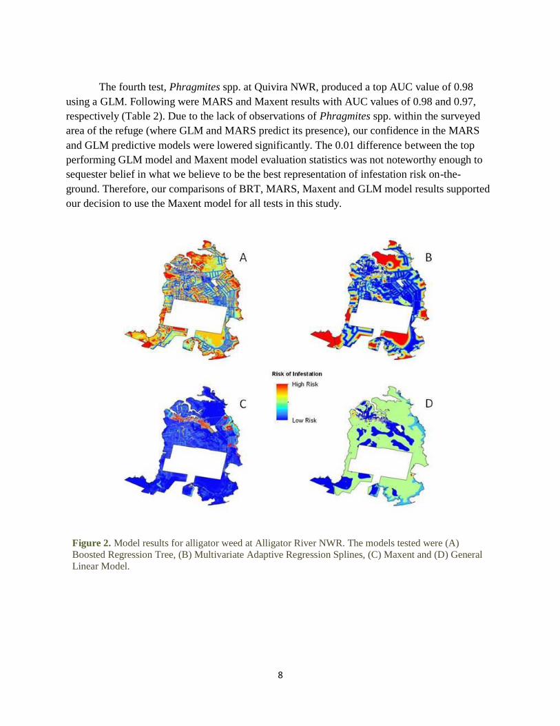
The fourth test, Phragmites spp. at Quivira NWR, produced a top AUC value of 0.98
using a GLM. Following were MARS and Maxent results with AUC values of 0.98 and 0.97,
respectively (Table 2). Due to the lack of observations of Phragmites spp. within the surveyed
area of the refuge (where GLM and MARS predict its presence), our confidence in the MARS
and GLM predictive models were lowered significantly. The 0.01 difference between the top
performing GLM model and Maxent model evaluation statistics was not noteworthy enough to
sequester belief in what we believe to be the best representation of infestation risk on-the-
ground. Therefore, our comparisons of BRT, MARS, Maxent and GLM model results supported
our decision to use the Maxent model for all tests in this study.
Figure 2. Model results for alligator weed at Alligator River NWR. The models tested were (A)
Boosted Regression Tree, (B) Multivariate Adaptive Regression Splines, (C) Maxent and (D) General
Linear Model.

9
Figure 3. Model results for tamarisk at Quivira NWR. The models tested were (A) Boosted Regression
Tree, (B) Multivariate Adaptive Regression Splines, (C) Maxent and (D) General Linear Model.
Final Models: Alligator River NWR and South Atlantic LCC
Within the Alligator River NWR boundaries, the Maxent model for alligator weed
predicted 7,649 acres at risk of invasion or approximately 3.5 % of the total refuge acreage. The
AUC evaluation was 0.98 with the distance from water having the most contribution to the final
model (Table 3). The model shows existing canals and other water sources as the area most at
risk (Figure 4). The model also predicted higher risk along highway 64 that runs east and west
across the refuge.
Table 3. The top three environmental predictors and their percent contribution for alligator weed in
Alligator River NWR.
Predictor Percent Contribution
Distance to Water 62.6%
Land Cover Type 20.7%
Slope 8%
10
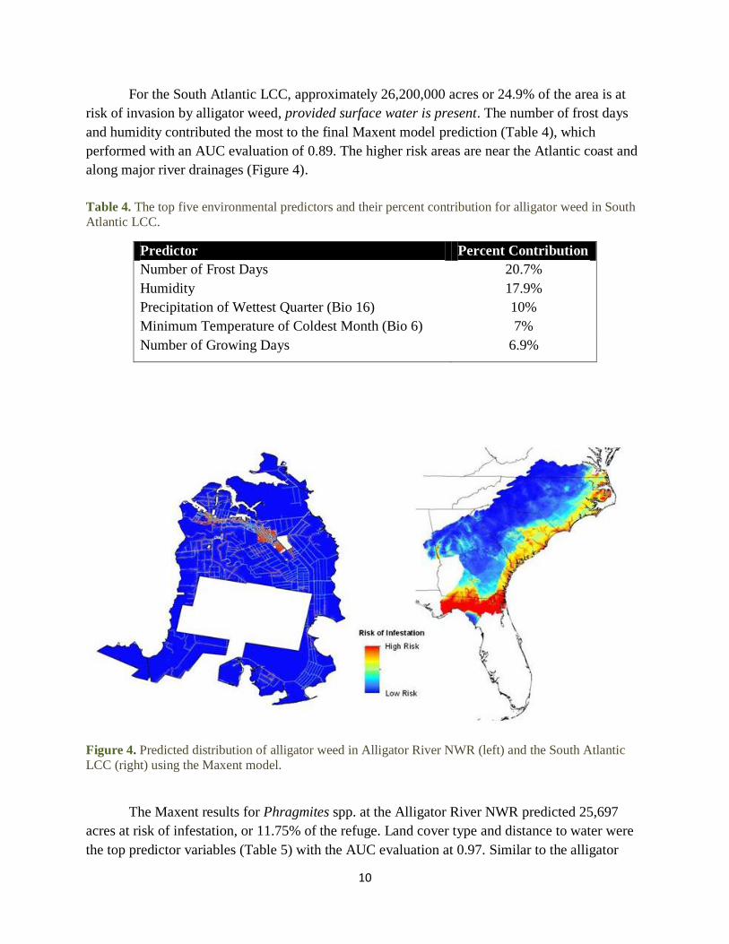
For the South Atlantic LCC, approximately 26,200,000 acres or 24.9% of the area is at
risk of invasion by alligator weed, provided surface water is present. The number of frost days
and humidity contributed the most to the final Maxent model prediction (Table 4), which
performed with an AUC evaluation of 0.89. The higher risk areas are near the Atlantic coast and
along major river drainages (Figure 4).
Table 4. The top five environmental predictors and their percent contribution for alligator weed in South
Atlantic LCC.
Predictor Percent Contribution
Number of Frost Days 20.7%
Humidity 17.9%
Precipitation of Wettest Quarter (Bio 16) 10%
Minimum Temperature of Coldest Month (Bio 6) 7%
Number of Growing Days 6.9%
Figure 4. Predicted distribution of alligator weed in Alligator River NWR (left) and the South Atlantic
LCC (right) using the Maxent model.
The Maxent results for Phragmites spp. at the Alligator River NWR predicted 25,697
acres at risk of infestation, or 11.75% of the refuge. Land cover type and distance to water were
the top predictor variables (Table 5) with the AUC evaluation at 0.97. Similar to the alligator

11
weed model, the predicted risk for Phragmites spp. was concentrated around existing canals and
water sources but showed a higher risk on the north east coast from Manns harbor south along
the Croatan sound (Figure 5).
Table 5. Top three environmental predictors and their percent contribution for Phragmites spp. in
Alligator River NWR.
Predictor Percent Contribution
Land Cover Type 35.9%
Distance to Water 32.1%
Prescribed Fire Treatment Areas 11.3%
For the South Atlantic LCC, approximately 35,500,000 acres or 33.7% of the area is at
risk of Phragmites spp. infestation. The Maxent model had an AUC evaluation of 0.79 with
mean diurnal range and solar radiation having greatest predictive contributions (Table 6). The
model predicted high risk near the coastal areas and further north in the LCC (Figure 5).
Table 6. Top five environmental predictors and their percent contribution for Phragmites spp. in South
Atlantic LCC.
Predictor Percent Contribution
Mean Diurnal Range (Bio 2) 20%
Radiation 18.6%
Elevation 17.3%
Geology 5.5%
Mean Temperature of Wettest Quarter (Bio 8) 5.1%

12
Figure 5. Predicted distribution of Phragmites spp. in Alligator River NWR (left) and the South Atlantic
LCC (right) using the Maxent model.
Final Models: Quivira NWR and Great Plains LCC
Within the Quivira NWR, the Maxent model predicted that 28,000 acres were at risk for
tamarisk invasion, or 49.5% of the refuge. The model had an AUC value of 0.82 with elevation,
soils and distance to water having almost equal contributions and the greatest predictive
contributions of all the predictors used to develop the model (Table 7). Higher risk areas were
predicted in the north and southeast near water sources and moist soils and along streams (Figure
6).
Table 7. Top three environmental predictors and their percent contribution for tamarisk in Quivira NWR.
Predictor Percent Contribution
Elevation 33.8%
Soil 27.7%
Distance to Water 23.3%
The Great Plains LCC, covering portions of 8 states, was predicted to have 48,700,000
acres, or 20.0% of the total area, at risk to tamarisk invasion. The model had an AUC value of
0.89 with distance to water and geology having the greatest predictive contributions (Table 8).
Model predictions of tamarisk risk at the Great Plans LCC were concentrated along river
corridors and higher in the west than east (Figure 6).

13
Table 8. Top five environmental predictors and their percent contribution for tamarisk in Great Plains
LCC.
Predictor Percent Contribution
Distance to Water 34.2%
Geology 16.7%
Radiation 11.1%
Precipitation of Wettest Quarter (Bio 16) 7.5%
Temperature Seasonality (Bio 4) 6.2%
Figure 6. Predicted distribution of tamarisk in Quivira NWR (left) and the Great Plains LCC (right) using
the Maxent model
For the Quivira NWR, Phragmites spp. predicted 3,617 acres or 12.9% of the total area at
risk to invasion. The Maxent results had an AUC value of 0.97 with the elevation, soil and land
cover type as the top three environmental predictor variables in the final model (Table 9). Areas
of predicted higher risk of Phragmites spp. were primarily in and around Little Salt Marsh and
nearby wetlands in the southern portion of Quivira NWR (Figure 7).

14
Table 9. Top three environmental predictors and their percent contribution for Phragmites spp. in Quivira
NWR.
Predictor Percent Contribution
Elevation 56.8%
Soil 18.6%
Land Cover Type 12.2%
For the Great Plains LCC, the model predicted that 142,200,000 acres or 58.5% of total
area was at risk to Phragmites spp.. The model results had a lower AUC value of 0.68 with
distance to water having the greatest predictive contribution (Table 10). Predicted risk for the
Great Plains LCC was distributed along river cooridros and showed higher risk in the norhter
portion of the LCC (Figure 7).
Table 10. The top five environmental predictors and their percent contribution for Phragmites spp. in
Great Plains LCC.
Predictor Percent Contribution
Distance to Water 36.2%
Frequency of Precipitation 12.2%
Temperature Annual Range (Bio 7) 9.5%
Temperature Seasonality (Bio 4) 7.2%
Mean Temperature of Wettest Quarter (Bio 8) 5.7%

15
Figure 7. Predicted distribution of Phragmites spp. in Quivira NWR (left) and the Great Plains LCC
(right) using the Maxent model.
Final Models: Silvio O. Conte NWR and North Atlantic LCC
Within the Silvio O. Conte NWR boundaries, the Maxent model for garlic mustard
predicted 1,150,000 acres at risk of invasion or approximately 45.5% of the total watershed
acreage. The AUC evaluation was 0.82 with the elevation having the most predictive
contribution (Table 11). Higher areas of risk were concentrated along major rivers and in the
southern portion of the NWR.
Table 11. The top three environmental predictors and their percent contribution for garlic mustard in
Silvio O. Conte NWR.
Predictor Percent Contribution
Elevation 49.2%
Soil 36.5%
Land Cover Type 10.3%
For the North Atlantic LCC, approximately 27,000,000 acres or 28.5% of the area is at
risk of infestation by garlic mustard (Figure 8). The maximum temperature and geology
contributed the most to the final Maxent model prediction (Table 12), which performed with an
AUC evaluation of 0.89.

16
Table 12. The top five environmental predictors and their percent contribution for garlic mustard in North
Atlantic LCC.
Predictor Percent Contribution
Max Temperature of Warmest Month (Bio 5) 29.3%
Maximum Temperature 13.1%
Geology 11.9%
Min Temperature of Coldest Month (Bio 6) 7.2%
Number of Growing Days 4.8%
Figure 8. Predicted distribution of garlic mustard in Silvio O, Conte NWR (left) and North Atlantic LCC
(right) using the Maxent model.
Within the Silvio O. Conte NWR watershed, the Maxent model predicted that 82,000
acres were at risk for Japanese stiltgrass invasion, or 22.7% of the refuge watershed. The
predicted area at risk was restricted to the south central portion of the NWR (Figure 9). The
model had an AUC value of 0.98 with elevation, soils, and distance to water having the greatest
predictive contributions (Table 13). The area of risk was
Risk of Infestation
High Risk
Low Risk
17
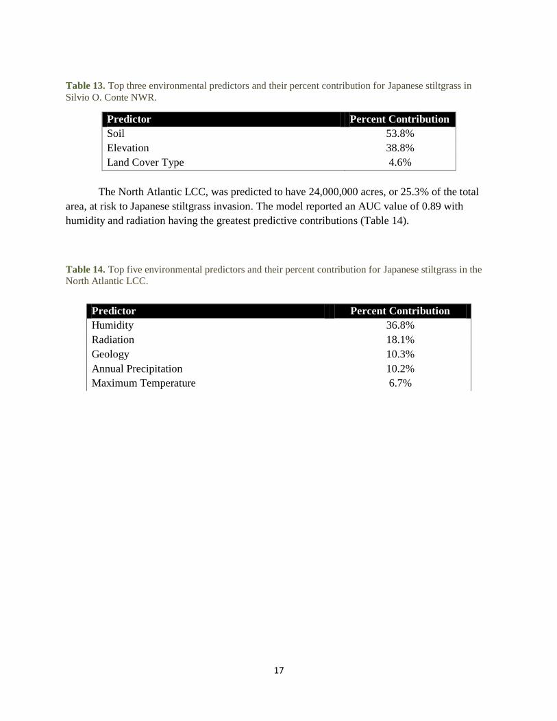
Table 13. Top three environmental predictors and their percent contribution for Japanese stiltgrass in
Silvio O. Conte NWR.
Predictor Percent Contribution
Soil 53.8%
Elevation 38.8%
Land Cover Type 4.6%
The North Atlantic LCC, was predicted to have 24,000,000 acres, or 25.3% of the total
area, at risk to Japanese stiltgrass invasion. The model reported an AUC value of 0.89 with
humidity and radiation having the greatest predictive contributions (Table 14).
Table 14. Top five environmental predictors and their percent contribution for Japanese stiltgrass in the
North Atlantic LCC.
Predictor Percent Contribution
Humidity 36.8%
Radiation 18.1%
Geology 10.3%
Annual Precipitation 10.2%
Maximum Temperature 6.7%

18
Figure 9. Predicted distribution of Japanese stiltgrass in in Silvio O, Conte NWR (left) North Atlantic
LCC (right) using the Maxent model.
Final Models: San Diego NWR and California LCC
At the San Diego NWR, false brome was predicted to be a potential risk for 4,658 acres
or 41.7% of the refuge. The Maxent model had an AUC value of 0.83 with soils as the top
contributing predictor to false brome’s distribution (Table 15). Areas of predicted higher risk of
false brome were throughout the western, northern and northeastern part of the refuge (Figure
10).
Table 15. Top three environmental predictors and their percent contribution for false brome in San Diego
NWR.
Predictor Percent Contribution
Soils
Land Cover Type
Slope
37.6%
20.8%
24.3%
The model of false brome at the California LCC scale predicted 19,188,000 acres or
29.7% of the LCC area is at risk for false brome. The humidity predictor had the largest
influence on the output, while the temperature seasonality had the second largest influence
(Table 16). False brome is projected to be distributed from San Diego to Los Angeles, around the
Bay Area, and west of the Sierra foothills within the Sacramento Valley (Figure 10).
Risk of Infestation
High Risk
Low Risk

19
Table 16. Top five environmental predictors and their percent contribution for false brome in the
California LCC.
Predictor Percent Contribution
Humidity 42.6%
Temperature Seasonality (bio 4) 21.2%
Distance to Water 11.4%
Precipitation of Seasonality (bio 15) 8.5%
Elevation 5.3%
The Sahara mustard is projected to encompass 1,722 acres of the San Diego NWR. This
equals 15.4% of the refuge Extent. For the mustard, the Maxent model had an AUC value of
0.88 with elevation being the top projector for the distribution (Table 17). Maxent projected
Sahara mustard to have a higher likelihood of occurrence in the northeastern part of the refuge.
Risk of Infestation
High Risk
Low Risk
Figure 10. Predicted distribution of false brome in San Diego NWR (left) and California LCC
(right) using the Maxent model.

20
Table 17. Top three environmental predictors and their percent contribution for Sahara mustard in San
Diego NWR.
Predictor Percent Contribution
Elevation
Soil
Land Cover Type
30.8%
26.2%
17.8%
The model for the Sahara mustard at the California LCC level predicted 17,129,000 acres
at risk, approximately 26.5% of the California LCC. Slope had the most influence of where the
Sahara mustard is projected, while the mean temperature of the wettest quarter also had the
second largest influence (Table 18). Sahara mustard has a higher risk of vitality on the Southern
California coastal environments (Figure 11).
Table 18. Top five environmental predictors and their percent contribution for Sahara mustard in the
California LCC.
Predictor Percent Contribution
Slope 58.0%
Mean Temperature of Wettest Quarter (bio 8) 14.2%
Mean Temperature of Coldest Quarter (bio 11) 11.9%
Number of Frost Days 5.3%
Annual Precipitation (bio 12) 2.6%

21
DISCUSSION
All Maxent models for the priority invasive species at the refuge and landscape scale
performed well with an AUC > 0.80. The results of these models provide maps showing
potential risk of the invasive species for the selected refuges and the associated LCCs. All
models used tested and proven statistical methods for model development and model evaluation.
These models also identified the environmental conditions that contribute the most to each
species potential distribution. In addition, the model results provide estimates of the area at risk
of invasion in terms of acres and proportion of modeled area for each species at both scales
(refuge and LCC). Although we tested multiple modeling techniques, only Maxent demonstrated
consistent performance.
The Maxent modeling method outperformed the presence-absence methods that were
tested in this report in both statistical evaluation and comparing model predictions to in the field
observed distributions. Even in the cases where the AUC for Maxent was not the highest, the
model predictions matched what was observed at the refuge much more accurately than the
higher statistically performing methods. The relatively poor performance of the other methods is
most likely due to the sampling design. Unlike Maxent, the presence-absence methods require
stricter sampling designs that fit the statistical designs to perform reliably (Cawsay et al., 2002).
While methods are being developed to generate suitable absence point for these presence-
absence methods (e.g., trend surface analysis; Acevedo et al., 2012), Maxent continues to be the
Risk of Infestation
High Risk
Low Risk
Figure 11. Predicted distribution of Sahara mustard in San Diego NWR (left) and California LCC (right)
using the Maxent model.
22
most appropriate modeling technique for this type of data (i.e., opportunistic sampling and
invasive species) collected for this report (Phillips et al., 2009).
Limitations of the quantity and/or the distribution of training data reduced model
performance for some species and scales (e.g., garlic mustard at Silvio O. Conte NWR and
Sahara mustard at the California LCC extent). While models still performed well in these
instances, additional data would likely increase the accuracy of model predictions. Furthermore,
for some of the refuges, there was little to no GIS data available which also constrained fine-
scale modeling (e.g., management activities, treatment). Although in these cases additional
environmental predictor variables were downloaded to supplement the model, there may have
been predictor variables that were not included that were importance drivers of the species
distribution.
Future efforts to model potential risk of invasive species using ecological niche models
should focus on collecting presence points that capture the spatial and environmental range of the
species of interest across the study area (Thuiller et al., 2004). Although the Maxent model can
handle a variety of collected data (e.g., observations, sample plots, historical records), we
strongly recommend that a system sampling strategy be considered for future efforts. By
sampling throughout each NWR and across the environmental range, predictions can be greatly
improved and be more informative. If absence data are collected, the presence-absence methods
for modeling potential distributions may also provide reliable predictions, but the issues of true
absences for invasive species are likely to still cause concern when interpreting model results
(Václavík and Meentemeyer, 2009).
CONCLUSION
Ecological niche models are commonly used to help anticipate and predict species
invasions across geographic scales (Peterson et al., 2003). At the refuge level, these results
provide statistically supported guidance for directing management initiatives, prioritizing early
detection/rapid response, and quantifying risk. For example, model predictions are often used to
prioritize search efforts to those areas with potentially higher invasion risk reducing the time and
area to search, while conserving economic and management resources. Furthermore, the
estimates of potential acres at risk in combination with the maps of predicted risk can provide
accepted risk assessments to inform policy makers on land-management decisions (Arriaga et al.,
2004), and be used to solicit funds for species specific management. As new species locations
are collected, additional and higher quality predictor layers are developed, and modeling
methods improve, distribution predictions can be iteratively updated to provide the most current
maps of invasive species risk.

23
ACKNOWLEDGEMENTS
We would like to acknowledge all of our US Fish and Wildlife Service collaborators
including Jenny Ericson, Lindy Gardner, Giselle Block and David Bishop; Brian VanDruten and
the staff at Alligator River NWR; Barry Parrish, Cynthia Boettner and the staff at Silvio O.
Conte NWR; Melanie Olds and the staff at Quivira NWR; and Pek Pum, John Martin and the
staff at San Diego NWR. We also thank Kimberly Edvarchuk from Utah State and her dedicated
field crew for their survey efforts at each refuge. Support for student interns was provided by
AmericaView through the ColoradoView Program housed at the Natural Resource Ecology
Laboratory at Colorado State University. Lastly, we thank our colleagues at the USGS Fort
Collins Science Center for advice and guidance during the modeling process, allowing us to test
and use the newly developed SAHM software to assist in model development, and hosting a
training seminar on Maxent modeling for the US Fish and Wildlife.

24
REFERENCES
Acevedo, P., A. Jiménez-Valverde, et al. (2012). "Delimiting the geographical background in
species distribution modeling." Journal of Biogeography 39(8): 1383-1390.
Allendorf, F. W. and L. L. Lundquist (2003). Introduction: Population Biology, Evolution, and
Control of Invasive Species. Conservation Biology 17(1): 24-30.
Arriaga, L., A. E. Castellanos V, et al. (2004). "Potential Ecological Distribution of Alien
Invasive Species and Risk Assessment: a Case Study of Buffel Grass in Arid Regions of
Mexico.” Conservation Biology 18(6): 1504-1514.
Brown, J.H., G.C. Stevens & D.M. Kaufman. 1996. The geographic range: size, shape,
boundaries, and internal structure. Annu. Rev. Ecol. Syst. 27: 597–623.
Cawsey, E. M., M. P. Austin, et al. (2002). "Regional vegetation mapping in Australia: a case
study in the practical use of statistical modeling." Biodiversity and Conservation 11(12):
2239-2274.
Elith, J., Leathwick, J.R. & Hastie, T. (2008). A working guide to boosted regression trees.
Journal of Animal Ecology 77:802-813.
Ellstrand, N. C. and K. A. Schierenbeck (2000). Hybridization as a stimulus for the evolution of
invasiveness in plants? Proceedings of the National Academy of Sciences 97(13):7043-
7050.
Evangelista, P. H., S. Kumar, et al. (2008). "Modelling invasion for a habitat generalist and a
specialist plant species." Diversity and Distributions 14(5): 808-817.
Evangelista, P., T. Stohlgren, et al. (2009). "Mapping Invasive Tamarisk (Tamarix): A
Comparison of Single-Scene and Time-Series Analyses of Remotely Sensed Data."
Remote Sensing 1(3): 519-533.
Ficetola, G. F., W. Thuiller, et al. (2007). "Prediction and validation of the potential global
distribution of a problematic alien invasive species — the American bullfrog." Diversity
and Distributions 13(4): 476-485.
Franklin, J. (2009). Mapping species distributions. Cambridge University Press.
Friedman, J.H. (1991). Multivariate adaptive regression splines. Annals of Statistics 19: 1-67.
Guisan, A., T. C. Edwards Jr, et al. (2002). Generalized linear and generalized additive models in
studies of species distributions: setting the scene. Ecological Modelling 157(2–3): 89-
100.
Hijmans, R. J. and C. H. Graham (2006). "The ability of climate envelope models to predict the
effect of climate change on species distributions." Global Change Biology 12(12): 2272-
2281.
Hutchinson, G. E. (1957). "Population Studies - Animal Ecology and Demography - Concluding
Remarks." Cold Spring Harbor Symposia on Quantitative Biology 22: 415-427.
Keller, R. P., D. M. Lodge, et al. (2007). "Risk assessment for invasive species produces net
bioeconomic benefits." Proceedings of the National Academy of Sciences 104(1): 203-
207.
Kumar, S., S. A. Spaulding, et al. (2009). "Potential habitat distribution for the freshwater diatom
Didymosphenia geminata in the continental US." 7(8): 415-420.

25
Mack, R. N., D. Simberloff, et al. (2000). "Biotic invasions: Causes, epidemiology, global
consequences, and control." Ecological Applications 10(3): 689-710.
Newbold, T. (2010). "Applications and limitations of museum data for conservation and ecology,
with particular attention to species distribution models." Progress in Physical Geography
34(1): 3-22.
Pearson, R. G., C. J. Raxworthy, et al. (2007). "Predicting species distributions from small
numbers of occurrence records: a test case using cryptic geckos in Madagascar." Journal
of Biogeography 34(1): 102-117.
Peterson, A T. (2003). "Predicting the Geography of Species’ Invasions via Ecological Niche
Modeling." The Quarterly Review of Biology 78(4): 419-433.
Phillips, S. J., M. Dudik, et al. (2004). A maximum entropy approach to species distribution
modeling. Proceedings of the twenty-first international conference on Machine learning.
Banff, Alberta, Canada, ACM: 83.
Phillips, S. J., R. P. Anderson, et al. (2006). "Maximum entropy modeling of species geographic
distributions." Ecological Modelling 190(3-4): 231-259.
Phillips, S. J., M. Dudík, et al. (2009). Sample selection bias and presence-only distribution
models: implications for background and pseudo-absence data. Ecological Applications
19(1): 181-197.
Pimentel, D., L. Lach, et al. (2000). "Environmental and Economic Costs of Nonindigenous
Species in the United States." Bioscience 50(1): 53-65.
Pimentel, D., R. Zuniga, et al. (2005). "Update on the environmental and economic costs
associated with alien-invasive species in the United States." Ecological Economics 52(3):
273-288.
Sinclair, S., White, M., and Newell, G. (2010). How useful are species distribution models for
managing biodiversity under future climates? Ecology and Society 15, Article 8.
Stohlgren, T. J. and J. L. Schnase (2006). "Risk analysis for biological hazards: What we need to
know about invasive species." Risk Analysis 26(1): 163-173.
Thuiller, W., L. Brotons, et al. (2004). "Effects of restricting environmental range of data to
project current and future species distributions." Ecography 27(2): 165-172.
Václavík, T. and R. K. Meentemeyer (2009). "Invasive species distribution modeling (iSDM):
Are absence data and dispersal constraints needed to predict actual distributions?"
Ecological Modelling 220(23): 3248-3258.
Yemshanov, D., F. H. Koch, et al. (2009). "Mapping Invasive Species Risks with Stochastic
Models: A Cross-Border United States-Canada Application for Sirex noctilio Fabricius."
Risk Analysis 29(6): 868-884.
York, P., P. Evangelista, et al. (2011). "A habitat overlap analysis derived from maxent for
tamarisk and the south-western willow flycatcher." Frontiers of Earth Science 5(2): 120-
129.

I
APPENDICES
Appendix 1. Predictor variables used to generate models at each refuge. The Source of the predictor
variable Land Cover Type varied from GAP (Quivira), DARE (Alligator River), and Landfire(Silvio O.
Conte), Vegetation 1995 (San Diego) depending on the refuge.
Predictor Alligator
River
Quivira Silvio O.
Conte
San
Diego
Aspect x x x x
Digital elevation model x x x x
Distance to water x x x x
Fire Management Areas x
Invasive Plant Management Areas x
Land Cover Type x x x x
Normalized Difference Vegetation Index (NDVI) x
Pretreatment areas x
Slope x x x x
Soils (USGS SURGO) x x x x
Vegetation Management x
Distance to road x

II
Appendix 2. Model results for Phragmites spp. at Alligator River NWR. The models tested were
(A) Boosted Regression Tree, (B) Multivariate Adaptive Regression Splines, (C) Maxent and (D)
General Linear Model.

III
Appendix 3. Model results for tamarisk at Quivira NWR. The models tested were (A) Boosted
Regression Tree, (B) Multivariate Adaptive Regression Splines, (C) Maxent and (D) General Linear
Model.

IV
Appendix 4. Model results for Japanese stiltgrass at Silvio O. Conte NWR. The models tested were
(A) Boosted Regression Tree, (B) Multivariate Adaptive Regression Splines, (C) Maxent and (D)
General Linear Model.