RESEARCH Open Access

Mapping behavioral specifications to modelparameters in synthetic biologyHeinz Koeppl1,2*, Marc Hafner3, James Lu4

From 10th International Workshop on Computational Systems BiologyTampere, Finland. 10-12 June 2013

Abstract

With recent improvements of protocols for the assembly of transcriptional parts, synthetic biological devices cannow more reliably be assembled according to a given design. The standardization of parts open up the way forin silico design tools that improve the construct and optimize devices with respect to given formal designspecifications. The simplest such optimization is the selection of kinetic parameters and protein abundances suchthat the specified design constraints are robustly satisfied. In this work we address the problem of determiningparameter values that fulfill specifications expressed in terms of a functional on the trajectories of a dynamicalmodel. We solve this inverse problem by linearizing the forward operator that maps parameter sets tospecifications, and then inverting it locally. This approach has two advantages over brute-force random sampling.First, the linearization approach allows us to map back intervals instead of points and second, every obtained valuein the parameter region is satisfying the specifications by construction. The method is general and can hence beincorporated in a pipeline for the rational forward design of arbitrary devices in synthetic biology.

IntroductionSynthetic biology places emphasis on small, standardizedmolecular parts and devices, mostly operating at the tran-scriptional level [1,2]. With standardization comes theneed for rigorous quantitative characterization of suchdevices and for a compositional theory to reliably buildlarger systems from small canonical circuits. For nowmost synthetic circuits implemented in vivo were con-structed from a small number of components with topol-ogy and parameter values found by trial-and-error. Thedevelopment of larger synthetic systems necessitates theuse of appropriate design methodologies. In silico analysescan provide significant insights into the construction ofcomplex synthetic systems, but due to the poor quantifica-tion of experimental and micro-environmental conditions,the predictive capability of in silico models for in vivoimplementations remains limited. Apart from experimen-tal limitations, modeling attempts to date most often makesimplifying assumptions about all the perturbations that asynthetic construct is facing in vivo. For instance, only a

few studies account for the large extrinsic noise [3-5] andin particular the one introduced by variations of plasmidcopy number [6]. Incorporating those realistic in vivo con-straints will make computational models more predictive,eventually enabling the upfront in silico optimization oftranscriptional circuits. A first step toward this goal is toinvestigate the parameter dependency of certain behavior-ial properties of a circuits. In systems biology attemptshave already been made to address this problem, however,they either rely on purely local measures [7,8] such as con-sidered in classical sensitivity analysis [9,10], or performrandom parameter sampling [11] to determined parameterdependencies.For a given circuit topology, kinetic parameters and

other parameters that are involved in controlling theexpression level of molecular species (e.g. promoter activ-ity or number of ribosome binding sites) are importantdesign parameters in synthetic biology. A major challengeis to find a set of parameters that satisfies the behavioralspecification of a device [12]. Computer science offers var-ious languages to formally define the proper functioningof a piece of code or hardware. Such specification lan-guages of formal verification are used to check important

* Correspondence: koeppl@ethz.ch1ETH Zurich, Zurich, SwitzerlandFull list of author information is available at the end of the article

Koeppl et al. BMC Bioinformatics 2013, 14(Suppl 10):S9http://www.biomedcentral.com/1471-2105/14/S10/S9

© 2013 Koeppl et al; licensee BioMed Central Ltd. This is an Open Access article distributed under the terms of the Creative CommonsAttribution License (http://creativecommons.org/licenses/by/2.0), which permits unrestricted use, distribution, and reproduction inany medium, provided the original work is properly cited.

behavioral properties, such as liveness, safety or fairness[13]. One convenient way to specify such properties is touse temporal logic, which is considered an extension ofclassical propositional reasoning, where propositional vari-ables may change their truth values over time. A promi-nent such logic is the linear temporal logic (LTL), wherethe truth value of the propositions is interpreted over alinear timeline [13]. Such techniques were already appliedto investigate robustness of computational models in sys-tem biology [14].Mathematically, the design problem is an inverse pro-

blem and hence inherits the general feature of such pro-blems, namely ill-posedness [15,16]. More specifically, fora certain behavioral specification one aims to find the cor-responding parameter set that gives rise to such behavior.An simple example for a quantity in feature space couldbe the concentration of a molecular species at particulartime-points. The problem is closely related to parameteroptimization and even more so to robust optimization,where an objective function - generally encoding somebehavioral constraint (e.g. making model trajectories closeto the measurements) - is optimized to yield the optimalparameter set. Ill-posedness refers to the observation thattwo close-by points in specification or behavioral featurespace may map to very distant points in the parameterspace, indicating that this mapping is generally not con-tractive but rather expansive. The inverse and correspond-ing forward problem is illustated in Figure 1.In the current analysis we restrict ourselves to models

obeying the reaction rate equation and hence constitute aset of nonlinear ordinary differential equations. In general,connected domains may map to disconnected domains,for instance if the dynamical system contains bifurcationpoints (e.g. see Figure 1). For the proposed linearizationapproach we will further restrict ourselves to connecteddomains in the respective image space. Moreover, we willnot resort to specifying behavior through temporal logicsbut will define general specification functionals. These aremappings ψ from an appropriate function space c ofn-dimensional trajectories (e.g. L2([0, T],Rn )) to them-dimensional reals and we choose the form

ψ(x) ≡∫ T

0g(s, x(s))ds

with x ∈ X and the feature kernel g : R≥0 × Rn≥0 → F ,

where F ⊆ Rm. A special and more tractable version of

the kernel is the convolution, i.e. g(t, x(t)) = h(T − t)x(t). Inthe following we will only require the map x ® g(·, x) to beonce-differentiable. With this, we can define the forwardmap from a p-dimensional parameter space to the featurespace as the composition F ≡ ψ ο �, with ϕ : Rp → X .The trajectories x ∈ X are generated by the reaction rateequation

ddt

x(t) = Nv(x(t), k) and x(0) = x0 ∈ Rn≥0, (1)

with the stoichiometric matrix N ∈ Zn × q, the reaction

flux vector v : Rn≥0 × R

p≥0 → R

q≥0 and k ∈ R

p≥0 the para-

meter set.

MethodsThe brute-force method of determining the parameterregion that satisfies a certain behavioral specificationS ⊆ F usually proceeds by Monte Carlo sampling of para-meter sets, generating corresponding trajectories accord-ing to (1), checking whether those satisfy S and finallyretaining only those parameter sets that led to satisfiedspecification S. There are two immediate downsides of thisapproach. First, most draws will be unsuccessful for highdimensional parameter spaces, for tight specifications, orfor both. Different approaches using an optimized sam-pling [11,17] have been developed to mitigate this pro-blem, but are not solving it as they require convergence ofthe sampling. Second, drawing parameter points in R

p

does not provide guarantees that those points belong to aconnected domain of consistent parameter sets. Here weprovide first attempts to tackle both problems.The main idea is to locally linearize the forward map F

around some point and then locally invert it. Hence, asmall enough local patch in feature space can be mappedbackward to a small patch in parameter space. By succes-sively sampling expansion points in their neighborhoods(e.g. by the ball-walk algorithm [18]) we can systemati-cally cover the entire specification S and obtain the corre-sponding parameter region. A series expansion of Faround some initial parameter set k0 reads

F(k0 + dk) = F(k0) +∂F(k)∂k

∣∣∣∣k=k0

dk + o(dk)

Defining df ≡ F (k0 + dk) − F (k0) we see that a neigh-borhood df in feature space to first order can bemapped backward using the Moore-Penrose pseudo-inverse

dk = L†df ,

that we define with care as

L† ≡ limλ→0

(LTL + λI)−1LT = limλ→0

L(LLT + λI)−1, (2)

where L denotes the linearized forward map andhence is just the m × p matrix

L ≡ ∂F(k)∂k

∣∣∣∣k=k0

. (3)

Note, that the limit in (2) exists even if the inverse ofLT L and LLT do not exist. Such situations are

Koeppl et al. BMC Bioinformatics 2013, 14(Suppl 10):S9http://www.biomedcentral.com/1471-2105/14/S10/S9

Page 2 of 7

encountered as soon as the number of specification fea-tures m are less than the number of parameters, i.e. thedimension p of the parameter space. Importantly, wecan compute (3) efficiently using the variational equa-tion for the system (1). Observe that

L =∂

∂kψ oϕ(k) =

∫ T

0

∂g(s, x)∂x

∣∣∣∣x=x(s,k)

∂x(s, k)∂k

∣∣∣∣k=k0

ds,

where the last terms in the integral is just the sensitivityof the solution of (1) to perturbations in k around k0.According to the variational equation the sensitivity obeysthe following ordinary n × pmatrix differential equation

ddt∂x(t, k)∂k

= N(∂v(x, k)∂x

∂x(t, k)∂k

+∂v(x, k)∂k

)with

∂x(0, k)∂k

= 0, (4)

where we skipped the explicit dependency on k0 forbrevity. Note, that (4) is equivalent to the transient sen-sitivity analysis of metabolic networks [9,10], proposedas an extension of classical metabolic control analysisthat only deals with steady state sensitivities. For a cer-tain k0 the sensitivity of the kernel g is a constant m × nmatrix that can be computed explicitly. Thus, by jointlysolving (1) and (4) for some k0 together with

ddt

L(t) =∂g(s, x)∂x

∣∣∣∣x=x(t,k0)

∂x(t, k)∂k

∣∣∣∣k=k0

with L(0) = 0

up to time T we obtain the linearized map L = L(T).Hence, for every sampled k0 and associated featurepoint f 0 we propose to design a feature ball

Bf 0(δ) = {f ∈ F | ||f − f 0||2 ≤ δ}and map it backward using L†. According to the sin-

gular value decomposition L† = UΣV with Σ a diagonalmatrix with non-negative entries [16], the backwardtransformation needs to be a sequence of a rotation, ascaling and another rotation and hence the image of Bf 0

under L† can only be a ellipsoid in the parameter space

{L†f |f ∈ Bf 0(δ)} ∈ Rp.

Clearly, sampling a multivariate region with balls ofsame dimension allow for a complete coverage of theregion - something that can only be extrapolated whenusing pointwise sampling [11]. The question to efficientlysample a region with balls has been addressed in compu-tational geometry and efficient randomized algorithmsare available [18].We remark that the map L is not the best local

approximation to F(k) in some norm sense. More speci-fically we can improve on L if we are giving additionalsamples of the neighborhood Bf 0(δ). Consider we drawanother ki ∈ Bk0, then we can construct a rank-oneupdate to L

Figure 1 (A) The forward problem of defining a parameter set from which trajectories and their behavioral features are computed. (B) Theinverse problem of finding a parameter regions for a predetermined behavioral specification region S. Columns from left to right correspond toparameter space, trajectory space and behavioral feature space, respectively. Connected convex sets can map to nonconvex non-connectedregions.

Koeppl et al. BMC Bioinformatics 2013, 14(Suppl 10):S9http://www.biomedcentral.com/1471-2105/14/S10/S9

Page 3 of 7

L̃i = L +�F − L�k

||�k||2 �kT (5)

where ΔF ≡ F(ki) − F(k0) and Δk ≡ ki − k0. In particular,the rank-one term (5) captures the nonlinear part of F.From (5) it follows that the matrix L̃i satisfies the consis-tency property

L̃i(ki − k0) = F(ki) − f 0. (6)

Thus, knowing how to construct rank-one updates overthe domain of interest is equivalent to knowing F(k)locally. In fact, L̃i is the matrix closest to L, with respect tothe Frobenius norm, that satisfies (6). Subsequently wewill use this improved linear approximation to F to boundthe error that one can incurrs if one uses the pseudoin-verse L† for the backward map. This will also providemeans to determine the maximal ball size δ to stay belowa certain error bound. We quantify the error in the featurespace by the backward map followed by a forward map.That is, we want to find a δ such that

||F (k0 + L† (

f − f 0)) − f ||2 ≤ ε (7)

for all f ∈ Bf 0(δ).Now suppose we know a bound r(δ) for the Frobenius

norm of the rank-one perturbation, i.e. ||L̃ − L||F ≤ ρ (δ)

in the local domain of interest. Note, that r(δ) could andneed to be estimated by sampling. Given a f i ∈ Bf 0 (δ) themaximal error of the inverse-forward map is

maxL̃:||L̃−L||F≤ρ(δ)

||L̃L† (f i − f 0) − (

f i − f 0) ||2

which is known from robust linear squares [16] to beequivalent to the error

||LL† (f i − f 0) − (

f i − f 0) ||2 + ρ (δ) ||L† (f i − f 0) ||2.

Assuming that L has linearly independent rows, LL† isthe identity matrix and thereby the error simplifies to

ρ (δ) ||L† (f i − f 0) ||2.

This result provides one way to determine the radiusof the feature ball δ when relying on the pseudo-inverse

max δδ

subject to

ρ (δ) ||L† (f − f 0) ||2 ≤ ε

||f − f 0||2 ≤ δ

(8)

ResultsAs a proof of concept of our method, we applied it to asimple synthetic sensor construct [19]. The system is

made of several gene copies (e.g. with plasmid transfec-tion), expressing a protein that dimerizes and activatesthe gene by binding to the promoter. In presence of theinhibitor (input of the system), the dimer is trapped andcannot bind to the promoter. A schematic of theinvolved reactions is depicted in Figure 2.The system is simulated according to mass-action and

obeys

dx1

dt= k1(x0

5 − x5) + k2x5 − k3x1

dx2

dt= k4x1 − 2k5x2

2 + 2k6x3 − k11x2

dx3

dt= k5x2

2 − k6x3 − k7x3y(t) + k8x4 − k9(x05 − x5)x3 + k10x5 − k11x3

dx4

dt= k7x3y(t) − k8x4 − k11x4

dx5

dt= k9(x0

5 − x5)x3 − k10x5 − k11x5.

(9)

where the states xi denote the concentration ofmRNA, protein, protein-dimer and dimer-promotercomplex, respectively. The quantities x0

5 and y(t) referthe total number of promoters and the external inhibi-tor concentration, respectively. The nominal value andthe meaning of the model parameters are summarizedin Table 1. We remark that such continuous state-spacemodel have their limitations for transcriptional circuitsbecause they require several gene copies in order toneglect the discrete Boolean nature of a single gene.For the specified behavioral features, we expect the

dimer to drop quickly after introduction of inhibitorand then quickly regain a high level after the inhibitor iswashed out of the medium. We also constrain themonomeric protein. The specification functionals arethe integral of the absolute difference to some targetvalue x* (s) for the monomer and the dimer concentra-tion over two small time intervals for each. More speci-fically,

[ψ1(x)ψ2(x)

]=

⎡⎢⎢⎢⎣

∫ T

0w1(s)[x2(s, k) − x∗

2(s)]2ds

∫ T

0w2(s)[x3(s, k) − x∗

3(s)]2ds

⎤⎥⎥⎥⎦ (10)

where w is the temporal weight function chosen to be

wi(t) ={

1 for t ∈ [t1, t2] ∪ [t3, t4]0 otherwise

for i = 1, 2(11)

The actual values for time-intervals for w1 and w2, aswell as the target values are shown together with thetrajectories for the nominal system (9) in Figure 3.For this case study we assume that we have means to

design the binding rate of the inhibitor to the dimer k7and the binding rate of the dimer to the promoter k9.To assess the error incurred by the linearization we con-sider the reverse-forward mapping as described in (7).

Koeppl et al. BMC Bioinformatics 2013, 14(Suppl 10):S9http://www.biomedcentral.com/1471-2105/14/S10/S9

Page 4 of 7

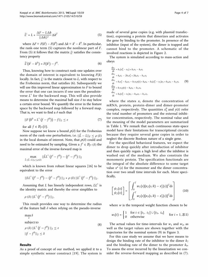
Hence for various size of δ we perform the inverse map-ping with L† and the forward mapping with F. If theinverse map is exact we should obviously obtain a ballwith the same δ. Any deviation ε thereof reflects theapproximation of F−1 by L†. In Figure 4 the images ofBf 0(δ) under L† and F ◦ L† are shown for various radii δ.Hence, for an intermediate size of δ a good trade-off

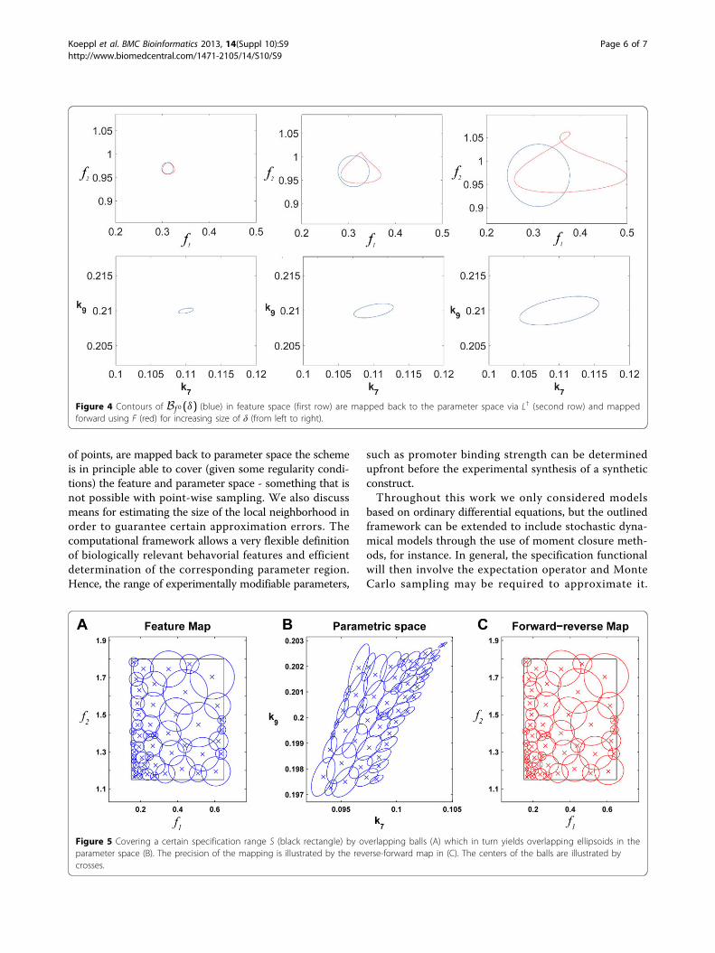
between approximation accuracy and sampling coverageis achievable. A systematic sampling of a predeterminedspecification area S would proceed by successively sam-pling overlapping balls with radii adapted to maintain εunder a certain value as illustrated in Figure 5. In thisexample, the coverage of the region S is above 98%using 50 balls of different radii. The lower left corner ofthe specification space (Figure 5A) maps to a stronglynonlinear region of the parameter space (upper right

corner in Figure 5B) and therefore forces the use ofsmaller balls to keep the error in acceptable range. Onthe contrary, the upper right region of the specificationspace is more linear and larger balls can be used withlimited relative error (Figure 5C).

ConclusionWe presented a novel method to determine the parameterregion of a biochemical reaction network that is consistentwith a certain dynamical, behavioral specification. Wedefined specifications in a novel and general way thatrequires only the specification map to be once differenti-able with respect to the states of the underlying differentialequations. We showed that by locally linearizing this mapwe can solve the desired inverse problem of finding a para-meter region for a given specification. As regions, instead

Figure 2 Simple transcriptional sensor construct. The dimerized form (A2) of a protein (A) is its own positive regulator; the inhibitor (I) tethersthe dimer away in an inactive form (A2 − I).

Table 1 Nominal values and meaning of the kineticparameters for the model of the synthetic sensorconstruct.

Basal transcription rate k1 0.02 sec−1

Active-promoter transcription rate k2 0.4 sec−1

mRNA degradation rate k3 0.3 sec−1

Protein translation rate k4 3 (nMsec) −1

Dimerization rate k5 0.1 (nMsec) −1

Dimer dissociation rate k6 0.001 sec−1

Inhibitor binding rate k7 0.011 (nMsec)−1

Inhibitor unbinding rate k8 0.2 sec−1

Dimer-promoter binding rate k9 0.21 (nMsec)−1

Dimer-promoter unbinding rate k10 0.2 sec−1

Protein degradation rate k11 0.2 sec−1

Values are based on [19] and slightly adapted to obtain a desired thresholdbehavior.

Figure 3 Time courses of monomer (A, x2) and dimer (A2, x3)concentration of (9) for an addition and removal of the inhibitor (I,y); the target values and time intervals chosen for the specificationfunctionals are indicated by solid black lines.

Koeppl et al. BMC Bioinformatics 2013, 14(Suppl 10):S9http://www.biomedcentral.com/1471-2105/14/S10/S9

Page 5 of 7

of points, are mapped back to parameter space the schemeis in principle able to cover (given some regularity condi-tions) the feature and parameter space - something that isnot possible with point-wise sampling. We also discussmeans for estimating the size of the local neighborhood inorder to guarantee certain approximation errors. Thecomputational framework allows a very flexible definitionof biologically relevant behavorial features and efficientdetermination of the corresponding parameter region.Hence, the range of experimentally modifiable parameters,

such as promoter binding strength can be determinedupfront before the experimental synthesis of a syntheticconstruct.Throughout this work we only considered models

based on ordinary differential equations, but the outlinedframework can be extended to include stochastic dyna-mical models through the use of moment closure meth-ods, for instance. In general, the specification functionalwill then involve the expectation operator and MonteCarlo sampling may be required to approximate it.

Figure 4 Contours of Bf 0(δ) (blue) in feature space (first row) are mapped back to the parameter space via L† (second row) and mappedforward using F (red) for increasing size of δ (from left to right).

Figure 5 Covering a certain specification range S (black rectangle) by overlapping balls (A) which in turn yields overlapping ellipsoids in theparameter space (B). The precision of the mapping is illustrated by the reverse-forward map in (C). The centers of the balls are illustrated bycrosses.

Koeppl et al. BMC Bioinformatics 2013, 14(Suppl 10):S9http://www.biomedcentral.com/1471-2105/14/S10/S9

Page 6 of 7

Methods from stochastic sensitivity analysis [20] can beapplied in order to perform the local inversion.

Competing interestsThe authors declare that they have no competing interests.

Authors’ contributionsHK, MH and JL devised the method, MH and JL implemented the algorithmand generated results for the case study. HK and MH wrote the paper.

DeclarationsPublication of this article was supported by the Swiss National ScienceFoundation (SNSF) grant number PP00P2_128503.This article has been published as part of BMC Bioinformatics Volume 14Supplement 10, 2013: Selected articles from the 10th International Workshopon Computational Systems Biology (WCSB) 2013: Bioinformatics. The fullcontents of the supplement are available online at http://www.biomedcentral.com/bmcbioinformatics/supplements/14/S10.

Authors’ details1ETH Zurich, Zurich, Switzerland. 2IBM Zurich Research Laboratory,Rueschlikon, Switzerland. 3Harvard Medical School, Boston MA, USA.4F. Hoffmann-La Roche, Basel, Switzerland.

Published: 12 August 2013

References1. Nandagopal N, Elowitz MB: Synthetic biology: integrated gene circuits.

Science (New York, NY) 2011, 333(6047):1244-8.2. Lu TK, Khalil AS, Collins JJ: Next-generation synthetic gene networks.

Nature Biotechnology 2009, 27(12):1139-50.3. Bowsher CG, Swain PS: Identifying sources of variation and the flow of

information in biochemical networks. Proceedings of the National Academyof Sciences of the United States of America 2012, 109(20):E1320-8.

4. Hilfinger A, Paulsson J: Separating intrinsic from extrinsic fluctuations indynamic biological systems. Proceedings of the National Academy ofSciences of the United States of America 2011, 108(29).

5. Zechner C, Ruess J, Krenn P, Pelet S, Peter M, Lygeros J, Koeppl H:Moment-based inference predicts bimodality in transient geneexpression. Proceedings of the National Academy of Sciences of the UnitedStates of America 2012, 109(21):8340-5.

6. Bleris L, Xie Z, Glass D, Adadey A, Sontag E, Benenson Y: Syntheticincoherent feedforward circuits show adaptation to the amount of theirgenetic template. Molecular Systems Biology 2011, 7(519):519.

7. Brown SK, Sethna JP: Statistical mechanical approach to models withmany poorly known parameters. Physical Review E 2003, , 68: 021904.

8. Gutenkunst RN, Waterfall JJ, Casey FP, Brown KS, Myers CR, Sethna JP:Universally Sloppy Parameter Sensitivities in Systems Biology Models.PLoS Comput Biol 2007, 3(10):e189.

9. Hatzimanikatis V, Bailey JE: MCA has more to say. Journal of TheoreticalBiology 1996, 182(3):233-42.

10. Ingalls BP, Sauro HM: Sensitivity analysis of stoichiometric networks: anextension of metabolic control analysis to non-steady state trajectories.Journal of Theoretical Biology 2003, 222:23-36.

11. Hafner M, Koeppl H, Hasler M, Wagner A: ’Glocal’ robustness analysis andmodel discrimination for circadian oscillators. PLoS Computational Biology2009, 5(10):e1000534.

12. Miller M, Hafner M, Sontag E, Davidsohn N, Subramanian S, Purnick PEM,Lauffenburger D, Weiss R: Modular Design of Artificial Tissue Homeostasis:Robust Control through Synthetic Cellular Heterogeneity. PLoS ComputBiol 2012, 8(7):e1002579.

13. Baier C, Katoen JP: Principles of Model Checking The MIT Press, London;2008.

14. Rizk A, Batt G, Fages F, Soliman S: Continuous valuations of temporallogic specifications with applications to parameter optimization androbustness measures. Theoretical Computer Science 2011,412(26):2827-2839.

15. Engl H, Hanke M, Neubauer A: Regularization of inverse problems,Mathematics and its applications Kluwer; 1996.

16. Christian HP: Rank-Deficient and Discrete Ill-Posed Problems Society forIndustrial and Applied Mathematics; 1998.

17. Zamora-Sillero E, Hafner M, Ibig A, Stelling J, Wagner A: Efficientcharacterization of high-dimensional parameter spaces for systemsbiology. BMC Systems Biology 2011, 5:142.

18. Vempala S: Geometric Random Walks: A Survey. Computational Geometry2005, 52:573-612.

19. Hooshangi S, Thiberge S, Weiss R: Ultrasensitivity and noise propagationin a synthetic transcriptional cascade. Proceedings of the National Academyof Sciences of the United States of America 2005, 102(10):3581-6.

20. Sheppard P, Rathinam M, Khammash M: A pathwise-derivative approachto the computation of parameter sensitivities in discrete stochasticchemical systems. Journal of Chemical Physics 2012, 136:034115.

doi:10.1186/1471-2105-14-S10-S9Cite this article as: Koeppl et al.: Mapping behavioral specifications tomodel parameters in synthetic biology. BMC Bioinformatics 201314(Suppl 10):S9.

Submit your next manuscript to BioMed Centraland take full advantage of:

• Convenient online submission

• Thorough peer review

• No space constraints or color figure charges

• Immediate publication on acceptance

• Inclusion in PubMed, CAS, Scopus and Google Scholar

• Research which is freely available for redistribution

Submit your manuscript at www.biomedcentral.com/submit

Koeppl et al. BMC Bioinformatics 2013, 14(Suppl 10):S9http://www.biomedcentral.com/1471-2105/14/S10/S9

Page 7 of 7