HAL Id: hal-01023050https://hal.inria.fr/hal-01023050

Submitted on 11 Jul 2014

HAL is a multi-disciplinary open accessarchive for the deposit and dissemination of sci-entific research documents, whether they are pub-lished or not. The documents may come fromteaching and research institutions in France orabroad, or from public or private research centers.

L’archive ouverte pluridisciplinaire HAL, estdestinée au dépôt et à la diffusion de documentsscientifiques de niveau recherche, publiés ou non,émanant des établissements d’enseignement et derecherche français ou étrangers, des laboratoirespublics ou privés.

Mapped Fourier Methods for stiff problems in toroidalgeometry

Herve Guillard

To cite this version:Herve Guillard. Mapped Fourier Methods for stiff problems in toroidal geometry. [Research Report]RR-8566, INRIA. 2014, pp.17. <hal-01023050>

ISS

N02

49-6

399

ISR

NIN

RIA

/RR

--85

66--

FR+E

NG

RESEARCHREPORTN° 8566July 2014

Project-Team Castor

Mapped Fourier Methodsfor stiff problems intoroidal geometryHervé Guillard

RESEARCH CENTRESOPHIA ANTIPOLIS – MÉDITERRANÉE

2004 route des Lucioles - BP 9306902 Sophia Antipolis Cedex

Mapped Fourier Methods for stiff problems intoroidal geometry

Hervé Guillard∗

Project-Team Castor

Research Report n° 8566 — July 2014 — 17 pages

Abstract: Fourier spectral or pseudo-spectral methods are usually extremely efficient for periodicproblems. However this efficiency is lost if the solutions have zones of rapid variations or internallayers. For these cases, a large number of Fourier modes are required and this makes the Fouriermethod unpractical in many cases. This work investigates the use of mapped Fourier methodas a way to circumvent this problem. Mapped Fourier method uses instead of the usual Fourierinterpolant the composition of the Fourier interpolant with a mapping in such a way that in thecomputational space, the functions to represent are not stiff. This work gives some examples ofthe usefulness of this method and apply it to a simple model of pellet injection in tokamaks as anexample of its potential interest for complex multi-dimensional problem.

Key-words: Spectral methods, Fourier approximation, mapped Fourier method, pellet injection,Tokamaks

∗ herve.guillard@inria.fr

Méthodes Spectrales Fourier transformées pour les problèmesraides en géométrie toroidale

Résumé : Les méthodes spectrales ou pseudo-spectrales de Fourier sont habituellement ex-trèmement efficaces pour les problèmes périodiques. Cette efficacité est cependant perduelorsque les solutions ont des zones localisées de variations rapides ou des couches internes.Dans ces cas, un grand nombre de modes de Fourier doit être utilisé pour représenter la solutionet les méthodes de Fourier deviennent inutilisables. Ce travail étudie l’utilisation des méthodesde Fourier transformées comme moyen de régler ce problème. Les méthodes de Fourier trans-formées utilisent à la place de l’interpolant de Fourier, la composition de cet interpolant avec unchangement de variables construit pour que dans l’espace de calcul, les fonctions à représen-ter n’aient pas de zones à variations rapides. Ce travail donne quelques exemples de l’utilitéde cette méthode et l’applique à un modèle simple d’injection de glaçons dans les tokamakscomme exemple de son intéret potentiel pour des problèmes complexes multidimensionnels.

Mots-clés : Méthodes Spectrales, Approximation de Fourier, méthode de Fourier transformée,injection de glaçon, Tokamaks

Mapped Fourier Methods in toroidal geometry 3

1 Introduction

Many problems in science and engineering involve one or several periodicity directions. Inthese directions, the numerical approximation of the mathematical models can be performed inan efficient way using Fourier decomposition of the solutions in term of trigonometric polyno-mials. For infinitely smooth solution, the convergence of Fourier methods is more rapid thanany finite power of 1/N where N is the number of Fourier modes : this property is called spec-tral accuracy and is one of the main advantage of Fourier methods versus finite difference (FD)or finite element (FE) local approximation methods since it allows to reach a very good accuracyusing a small number of modes. Moreover, the existence of fast algorithms (Fast Fourier Trans-form) commonly available on vector and parallel computers allows an efficient implementationof these method in term of CPU cost.Therefore in different branches of science and engineering, a large number of simulation codesrely on the use of Fourier techniques. This is for instance the case in astrophysics or in plasmaphysics and tokamak research where mature simulation codes designed, validated and tunedagainst experimental and observational results are used in a routine or production way in manydifferent teams worldwide.However, all these advantages of Fourier methods break down if the solution possesses local-ized internal layers and region of rapid changes which are small in comparison of the compu-tational domain. For these cases, even if the solution is infinitely smooth1, spectral accuracy isonly recovered for a large number of Fourier modes, making the use of these methods unprac-tical.To simulate these cases, one possibility is to use local FD/FE methods. However, this can implya large re-coding effort that is not always possible due to time and money constraints. Anotherpossibility is to alter the physics of the problem by enlarging artificially the region of large vari-ations or modifying the governing parameters of the problem to obtain a less stiff problem. Forcomplex problem governed by non linear partial differential equation, the correctness of theresults obtained in this way is not guaranteed.In this work, we experiment another possibility whose advantage is to not require large modi-fication of existing codes. Only the parts of the code performing the computations of the spatialderivatives in the periodicity directions need to be changed and moreover these modificationscan be light (depending of the structure of the existing code however). The basic idea is tochange the global trigonometric interpolant by functions much more adapted to the represen-tation of functions exhibiting rapid internal variations. This is done by composing the Fouriermodes with an appropriate change of variables. Another way to present the same idea is towrite the initial problem in a computational domain where the solution is not stiff.This idea to use a change of variable to map a physical domain to a periodic one for compu-tational purpose is not new. The term mapped Fourier methods to designate these methodshave been used in quantum computations studies [5] almost 20 years ago and it is for instancediscussed at length in the well-known Boyd’s text book [3]. In the cases where the localizationof the internal zones of rapid variations is not know but is part of the problem, algorithms toconstruct an adapted mapping from the knowledge of the current solution or of the residualhave been designed see [7] and [1]. For some theoretical development on the convergence ofthese type of methods in a non-periodic context, one can consult [10, 11].The structure of this paper is as follows. In section 2, we give some examples of the behaviorof Fourier methods when the solutions exhibit localized internal layers to emphasize the loss of

1The case where the solution possesses shocks or discontinuities is different : for shock, spectral accuracy is neverrecovered, even if N is very large. The present work does not address this problem and concentrates on problems withsmooth solutions.

RR n° 8566

4 H.Guillard

fast convergence of Fourier methods in these problems. Section 3 recall the principle of mappedFourier methods and revisits the examples given in section 2 to show the potentialities of themethod. Section 4 apply this technique for the simulation of a crude model of pellet injection, atechnique used to refuel the core plasma in tokamaks. Finally we conclude by some remarks.

2 Spectral accuracy and spatial resolution

2.1 Accuracy of the numerical derivatives

We begin with the very simple problem of computing the successive derivatives of a functionpossessing a region of rapid variation. The test function considered is the Maxwellian :

u(x) = e−(x−π)2

∆2

Computing the derivatives of this function by a Fourier method is done by sampling u on a setof discrete points xj = 2π/N, j = 0, . . . , N−1 and replacing u by its Fourier interpolant INu thatis a member of SN the set of trigonometric polynomials of degree N . The Fourier interpolant isdefined by

INu =N/2−1∑k=−N/2

ukeikx

where the coefficients u are computed by the Discrete Fourier Transform (DFT):

uk =1N

N−1∑j=0

u(xj)e−ikxj

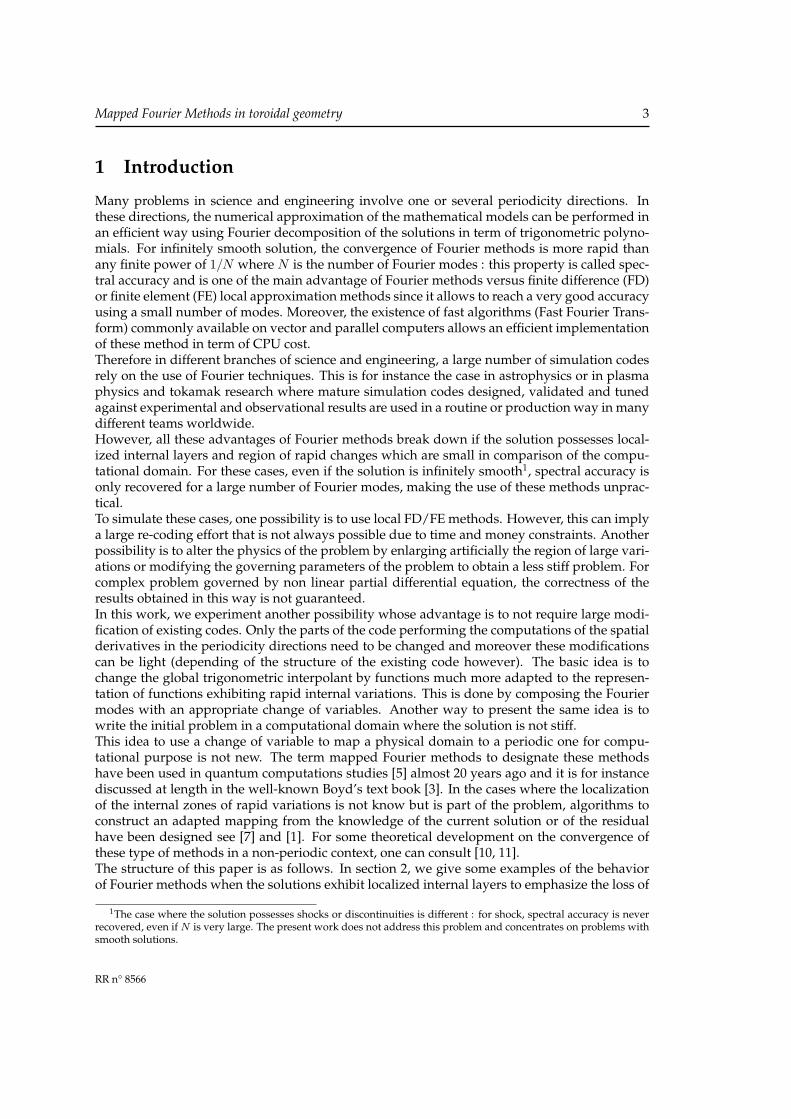
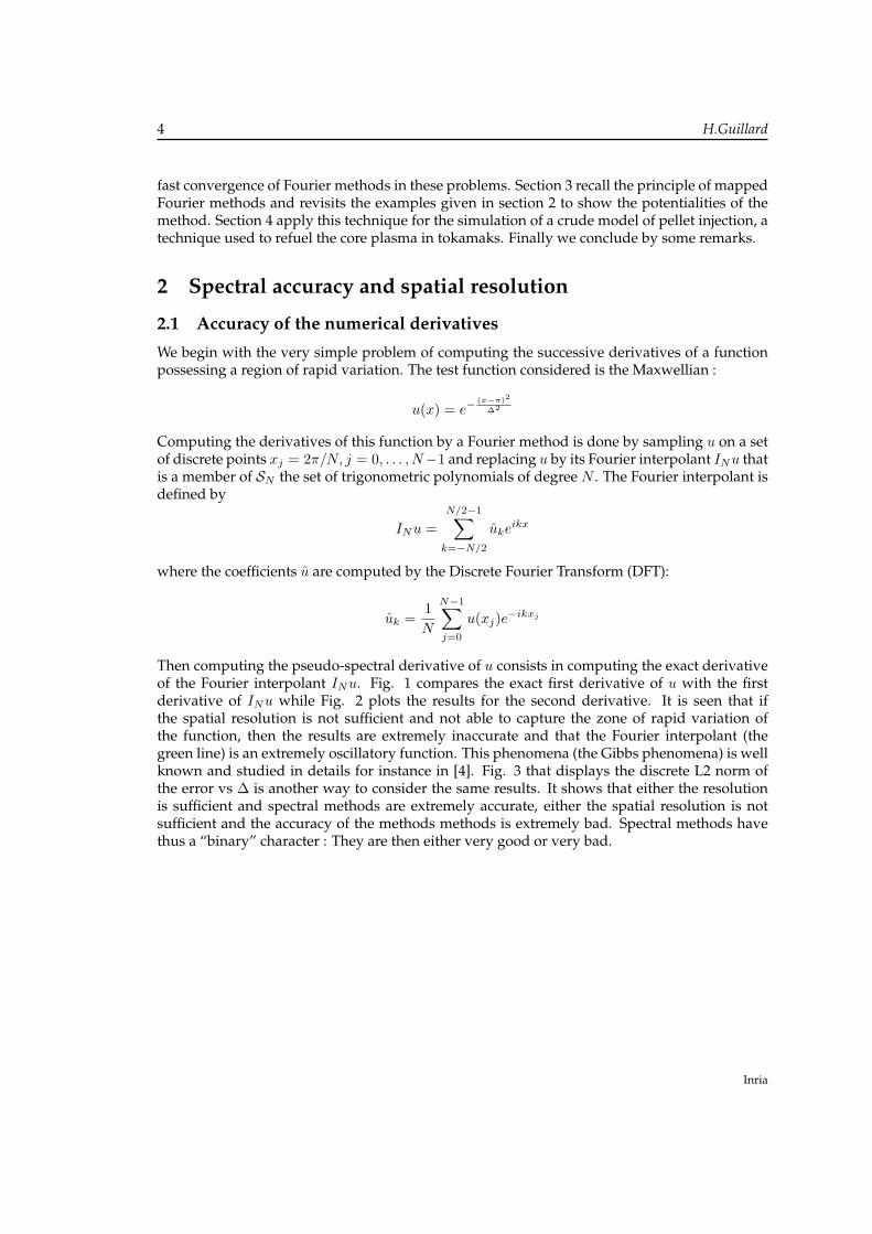
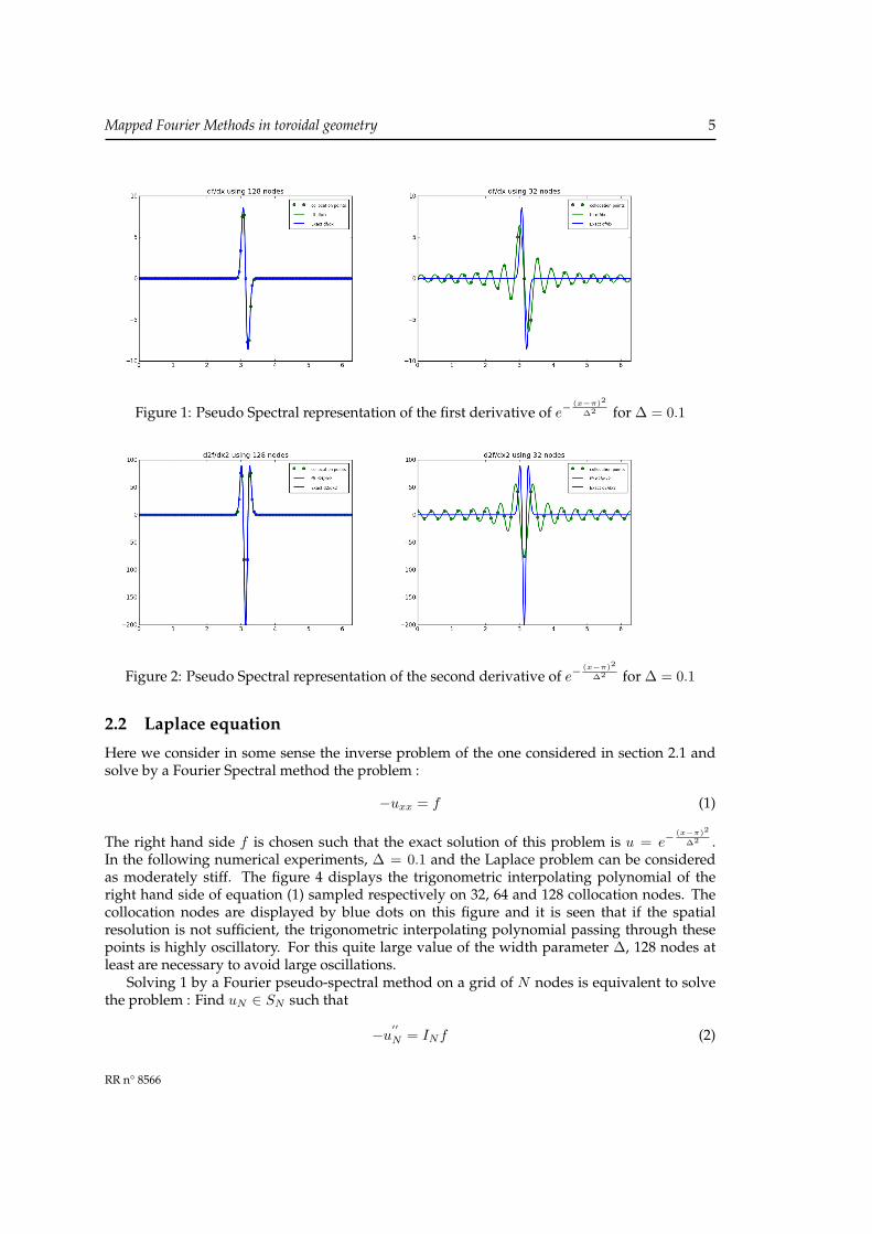
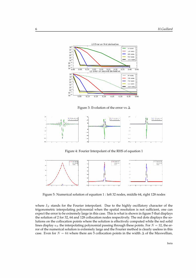
Then computing the pseudo-spectral derivative of u consists in computing the exact derivativeof the Fourier interpolant INu. Fig. 1 compares the exact first derivative of u with the firstderivative of INu while Fig. 2 plots the results for the second derivative. It is seen that ifthe spatial resolution is not sufficient and not able to capture the zone of rapid variation ofthe function, then the results are extremely inaccurate and that the Fourier interpolant (thegreen line) is an extremely oscillatory function. This phenomena (the Gibbs phenomena) is wellknown and studied in details for instance in [4]. Fig. 3 that displays the discrete L2 norm ofthe error vs ∆ is another way to consider the same results. It shows that either the resolutionis sufficient and spectral methods are extremely accurate, either the spatial resolution is notsufficient and the accuracy of the methods methods is extremely bad. Spectral methods havethus a “binary” character : They are then either very good or very bad.

Inria

Mapped Fourier Methods in toroidal geometry 5

Figure 1: Pseudo Spectral representation of the first derivative of e−(x−π)2

∆2 for ∆ = 0.1

Figure 2: Pseudo Spectral representation of the second derivative of e−(x−π)2

∆2 for ∆ = 0.1

2.2 Laplace equation

Here we consider in some sense the inverse problem of the one considered in section 2.1 andsolve by a Fourier Spectral method the problem :

−uxx = f (1)

The right hand side f is chosen such that the exact solution of this problem is u = e−(x−π)2

∆2 .In the following numerical experiments, ∆ = 0.1 and the Laplace problem can be consideredas moderately stiff. The figure 4 displays the trigonometric interpolating polynomial of theright hand side of equation (1) sampled respectively on 32, 64 and 128 collocation nodes. Thecollocation nodes are displayed by blue dots on this figure and it is seen that if the spatialresolution is not sufficient, the trigonometric interpolating polynomial passing through thesepoints is highly oscillatory. For this quite large value of the width parameter ∆, 128 nodes atleast are necessary to avoid large oscillations.

Solving 1 by a Fourier pseudo-spectral method on a grid of N nodes is equivalent to solvethe problem : Find uN ∈ SN such that

−u′′

N = INf (2)

RR n° 8566

6 H.Guillard

Figure 3: Evolution of the error vs ∆

Figure 4: Fourier Interpolant of the RHS of equation 1

Figure 5: Numerical solution of equation 1 : left 32 nodes, middle 64, right 128 nodes

where IN stands for the Fourier interpolant. Due to the highly oscillatory character of thetrigonometric interpolating polynomial when the spatial resolution is not sufficient, one canexpect the error to be extremely large in this case. This is what is shown in figure 5 that displaysthe solution of 2 for 32, 64 and 128 collocation nodes respectively. The red dots displays the so-lutions on the collocation points where the solution is effectively computed while the red solidlines display uN the interpolating polynomial passing through these points. For N = 32, the er-ror of the numerical solution is extremely large and the Fourier method is clearly useless in thiscase. Even for N = 64 where there are 5 collocation points in the width ∆ of the Maxwellian,

Inria

Mapped Fourier Methods in toroidal geometry 7

small oscillations can be noticed in the solution and at least 128 are needed to solve this problemwith a sufficient accuracy.

3 Mapped Fourier methods

3.1 Principle of the method

Consider a partial differential equation on [0, 2π] that we write symbolically as

L(u,∂u

∂x,∂2u

∂x2, . . . ) = f (3)

The principle of Fourier methods is to look for the solution u of this PDE in the space SN of thetrigonometric polynomials of order N . Although there are many variations of spectral methods(Galerkin, Tau, collocation), a common characteristics of Fourier methods is to compute theapproximate solution by sampling u (or the RHS f ) on a set of discrete points xj = 2π/N, j =0, . . . , N − 1 and to replace it by its Fourier interpolant

INu =N/2−1∑k=−N/2

ukTk(x)

where the basis functions Tk = eikx are the Fourier modes and where the coefficients u arecomputed by the Discrete Fourier Transform (DFT):

uk =1N

N−1∑j=0

u(xj)e−ikxj

As shown in section 2 a drawback of this type of method is that the Fourier modes are unableto represent a function displaying small localized features when the spatial resolution is notsufficient : either the resolution is sufficient and Fourier methods are extremely efficient andaccurate, either the spatial resolution is not sufficient and the accuracy of Fourier methods isextremely low.Since the Fourier modes are not adapted to the representation of stiff functions with localizedfeatures, a simple remedy is simply to change the Fourier modes for functions that are betteradapted to the characteristics of the functions that are to be computed. This can be simplydone by introducing a smooth change of variables h : ξ → x and to consider instead of theFourier modes Tk(x), mapped Fourier modes defined by Tk o h−1(x). The function u(x) is thendeveloped on the basis of the mapped Fourier modes :

IN (h)u =N/2−1∑k=−N/2

ukTk o h−1(x)

and standard (Galerkin or collocation) methods can be used as with usual methods.

Another way to describe this technique is to consider that to each function u(x) defined onΩx = [0, 2π] is associated another function U(ξ) defined on a computational space Ωξ by :

U(ξ) = u(x(ξ)) = u o h(ξ)

RR n° 8566

8 H.Guillard

The mapping h is chosen to provide an adequate resolution in the computational space Ωξ or inother words, such that the function U(ξ) is not stiff. The solution u(x) of (3) can then be obtainedfrom the solution of the transformed pde

Lξ(u,∂U∂ξ

,∂2u

∂ξ2, . . . ) = fξ (4)

obtained from repeated application of the chain rule to the partial derivatives present in (3).Equation (4) is then discretized using a standard Fourier method. This procedure can lookdifficult to implement as the pde (4) can be considerably more complex than (3) especially if (3)contains high order derivatives.However if a collocation method is used, to solve (3), only the expression of the derivativesat the collocation points xj are needed. Then, let D be the matrix representing the Fourierderivative at the collocation points, i.e

(INu)′(xi) =∑

Diju(xj)

and denote u (resp U ) the N-dimensional vector of the values of u at the collocation points xii.e ui = u(xi) (resp. the N-dimensional vector of the values of U at the collocation points ξi i.eU i = U(ξi) ) then the application of the chain rule give :

u′(xj) =U ′(ξj)h′(ξj)

=1

h′(ξj)(DU)j =

1h′(ξj)

(Du)j (5)

since u(xj) = U(ξj) and the vectors U and u are identical. The mapped Fourier technique thusreduces to multiply by a diagonal matrix the result of the standard Fourier derivative. Thislast operation is usually done without assembling the matrix D and using instead Fast FourierTransform.Let us now consider the evaluation of higher order derivatives, one possibility is to evaluatethem using the Faà di Bruno formula. For instance, we have

u′′(xj) =1

(h′(ξj))3[h′(ξj)U ′′(ξj)− h′′(ξj)U ′(ξj)] (6)

and U ′′(ξj) can be evaluated as U ′(ξj) by FFT. However, an alternate way to evaluate high orderderivatives is simply to apply in a repeated way the expression (5). This is the strategy that hasbeen followed in this paper.In the following two sections, we repeat the numerical experiments of sections 2.1 and 2.2 todemonstrate the benefits of using mapped Fourier methods. The mapping considered is

x = h(ξ) = atan(Ltanξ) (7)

Use of this mapping has been proposed and advocated in [2] that gives good arguments toprefer it against alternate choices in the periodic case.

3.2 Accuracy of the numerical derivatives

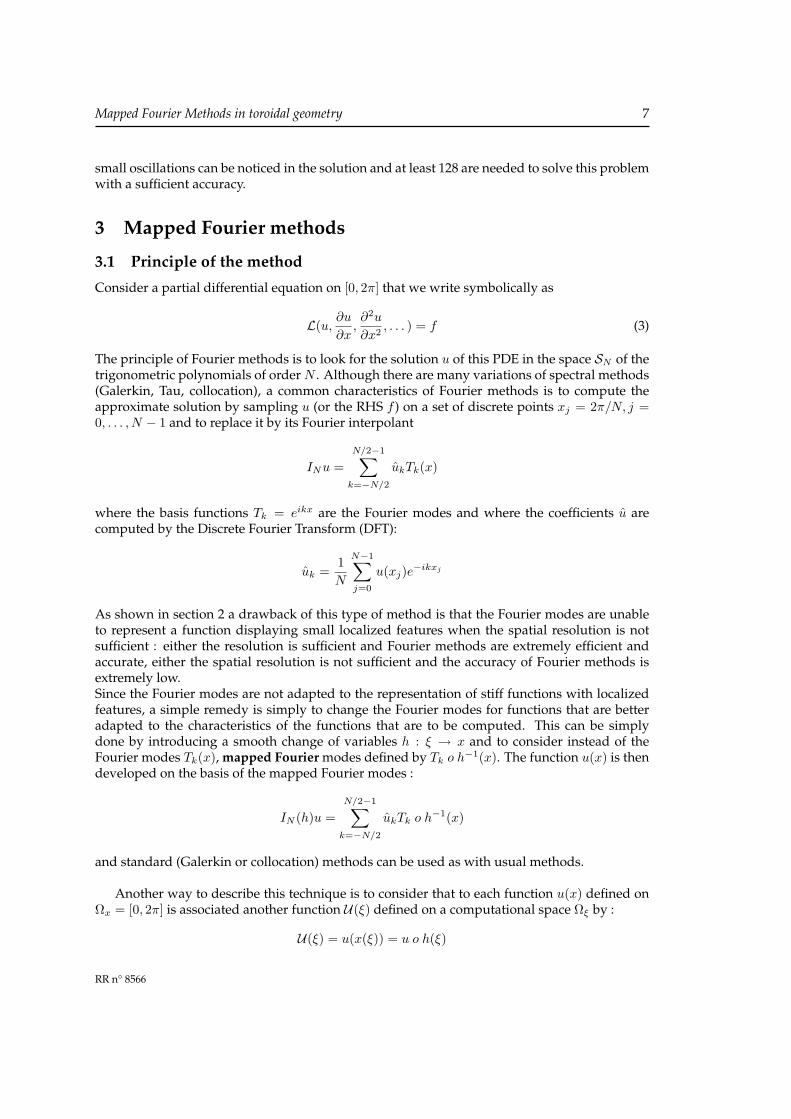
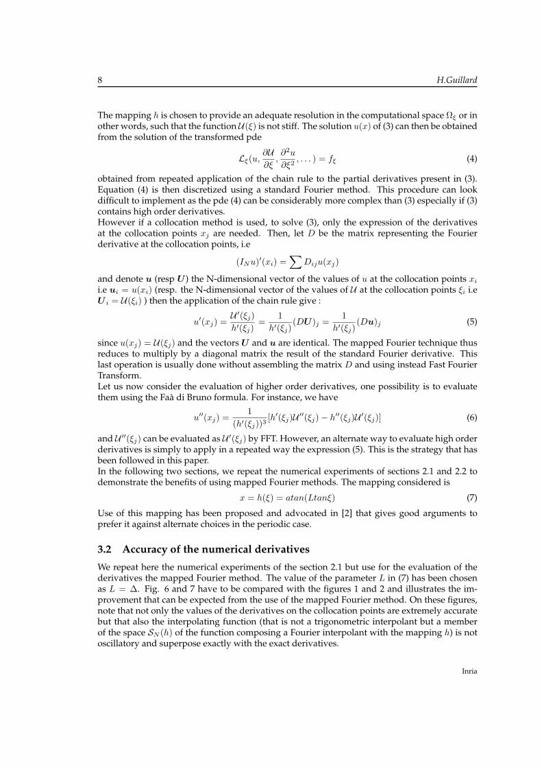
We repeat here the numerical experiments of the section 2.1 but use for the evaluation of thederivatives the mapped Fourier method. The value of the parameter L in (7) has been chosenas L = ∆. Fig. 6 and 7 have to be compared with the figures 1 and 2 and illustrates the im-provement that can be expected from the use of the mapped Fourier method. On these figures,note that not only the values of the derivatives on the collocation points are extremely accuratebut that also the interpolating function (that is not a trigonometric interpolant but a memberof the space SN (h) of the function composing a Fourier interpolant with the mapping h) is notoscillatory and superpose exactly with the exact derivatives.

Inria

Mapped Fourier Methods in toroidal geometry 9

Figure 6: Mapped Fourier representation of the first derivative of e−(x−π)2

∆2 for : left plot ∆ = 0.1,right plot ∆ = 0.01, note that the right plot is a zoom on the central region

Figure 7: Mapped Fourier representation of the second derivative of e−(x−π)2

∆2 for : left plot∆ = 0.1, right plot ∆ = 0.01, note that the right plot is a zoom on the central region

3.3 Laplace equation

In this section, we again consider the solution of equation (1). The exact solution is the Maxwellian

u = e−(x−π)2

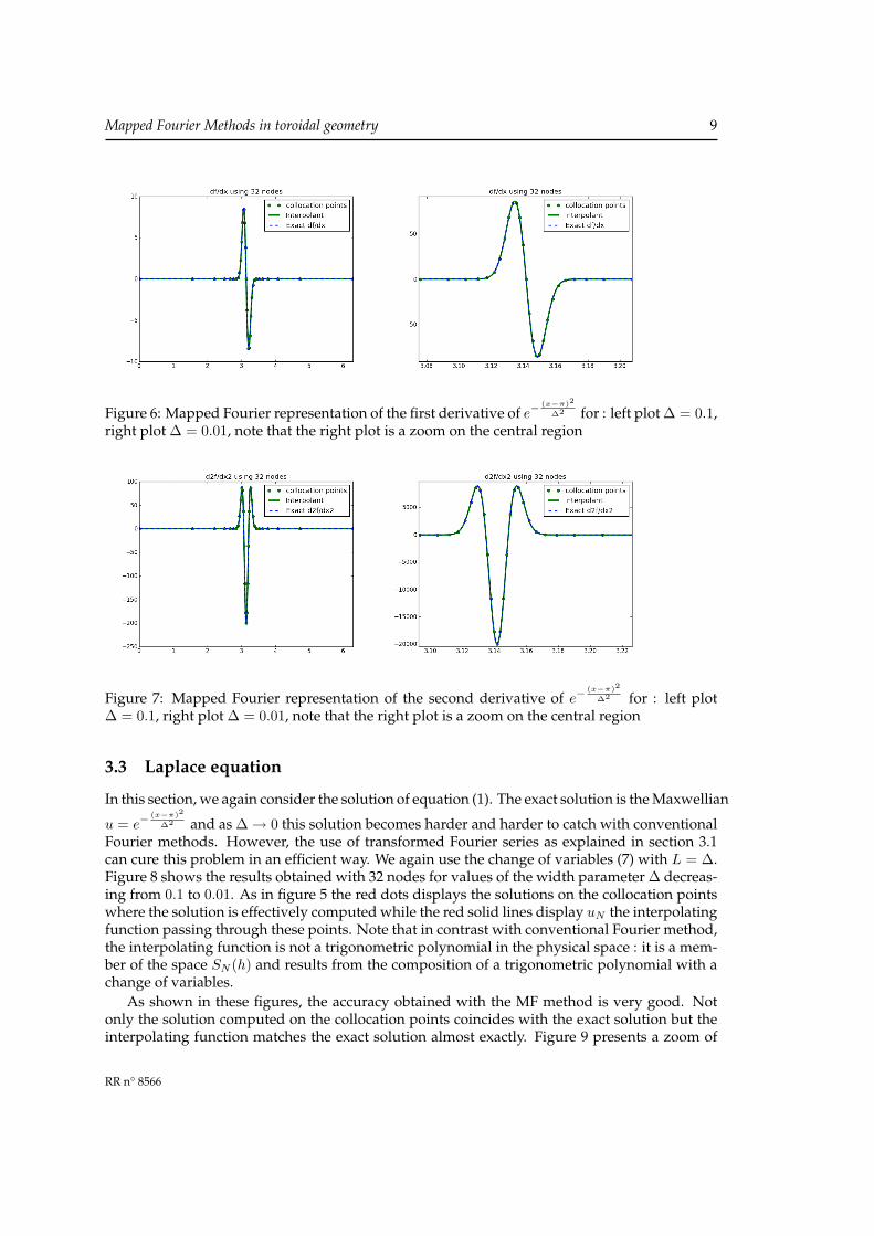
∆2 and as ∆→ 0 this solution becomes harder and harder to catch with conventionalFourier methods. However, the use of transformed Fourier series as explained in section 3.1can cure this problem in an efficient way. We again use the change of variables (7) with L = ∆.Figure 8 shows the results obtained with 32 nodes for values of the width parameter ∆ decreas-ing from 0.1 to 0.01. As in figure 5 the red dots displays the solutions on the collocation pointswhere the solution is effectively computed while the red solid lines display uN the interpolatingfunction passing through these points. Note that in contrast with conventional Fourier method,the interpolating function is not a trigonometric polynomial in the physical space : it is a mem-ber of the space SN (h) and results from the composition of a trigonometric polynomial with achange of variables.

As shown in these figures, the accuracy obtained with the MF method is very good. Notonly the solution computed on the collocation points coincides with the exact solution but theinterpolating function matches the exact solution almost exactly. Figure 9 presents a zoom of

RR n° 8566

10 H.Guillard

Figure 8: Numerical solution of equation (1) with 32 nodes : left ∆ = 0.1, middle ∆ = 0.05,right ∆ = 0.01

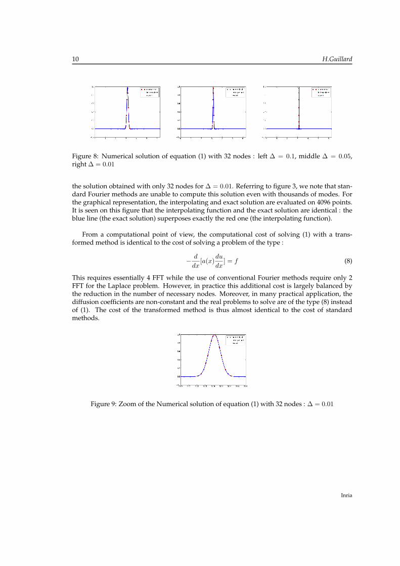
the solution obtained with only 32 nodes for ∆ = 0.01. Referring to figure 3, we note that stan-dard Fourier methods are unable to compute this solution even with thousands of modes. Forthe graphical representation, the interpolating and exact solution are evaluated on 4096 points.It is seen on this figure that the interpolating function and the exact solution are identical : theblue line (the exact solution) superposes exactly the red one (the interpolating function).

From a computational point of view, the computational cost of solving (1) with a trans-formed method is identical to the cost of solving a problem of the type :

− d

dx[a(x)

du

dx] = f (8)

This requires essentially 4 FFT while the use of conventional Fourier methods require only 2FFT for the Laplace problem. However, in practice this additional cost is largely balanced bythe reduction in the number of necessary nodes. Moreover, in many practical application, thediffusion coefficients are non-constant and the real problems to solve are of the type (8) insteadof (1). The cost of the transformed method is thus almost identical to the cost of standardmethods.

Figure 9: Zoom of the Numerical solution of equation (1) with 32 nodes : ∆ = 0.01

Inria

Mapped Fourier Methods in toroidal geometry 11

4 Pellet Injection

In magnetic confinement experiments for fusion research, the injection of cryogenic DT pelletin the plasma is considered as one of the most interesting way to fuel the core plasma. Pelletswhich are composed of neutral gas are rapidly heated by the plasma electrons and ionize to re-fuel the plasma. Moreover present tokamaks based on the so-called H-mode regime are knownto be subject to some kind of MHD instabilities known as ELMs for Edge Localized Modes thatcan cause an excessive erosion of the plasma facing component. The triggering of ELMS bypellet injection has been demonstrated experimentally to be a possible technique to reduce theamplitude of naturally occurring large ELMs. However, a lot of uncertainties remains for thepractical application of this technique in the future ITER tokamak and reliable numerical sim-ulations can be extremely useful to reduce these uncertainties. The simulation of this problemis complex and involves the coupling of a non-linear MHD model with a pellet ablation model.This is usually done by introducing in the MHD model a density source term to model the ab-lation of the pellet. One of the difficulties of this type of simulation comes from the fact that thepellet size is much smaller than the tokamak size. A typical ratio of these dimensions is of order10−3. Consequently the number of numerical simulations for this type of problem is relativelysmall : Among the few works devoted to this question one can notice the work of Samtaney etal [9] that use AMR technique to deal with the size problem or Futatani et al [6] that artificiallyincrease the pellet size.In this preliminary work, we do not intend to use a complex MHD model to deal with thisquestion but rather we want to study how the use of mapped Fourier methods can help to dealwith this problem.

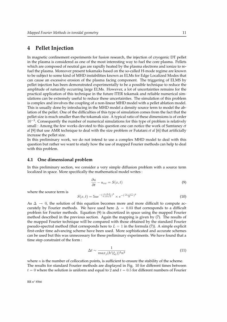
4.1 One dimensional problem

In this preliminary section, we consider a very simple diffusion problem with a source termlocalized in space. More specifically the mathematical model writes :

∂u

∂t− uxx = S(x, t) (9)

where the source term isS(x, t) = 5ue−( t−0.3

0.15√

2)2 × e−(

(x−π))∆ )2 (10)

As ∆ → 0, the solution of this equation becomes more and more difficult to compute ac-curately by Fourier methods. We have used here ∆ = 0.03 that corresponds to a difficultproblem for Fourier methods. Equation (9) is discretized in space using the mapped Fouriermethod described in the previous section. Again the mapping is given by (7). The results ofthe mapped Fourier technique will be compared with those obtained by the standard Fourierpseudo-spectral method (that corresponds here to L = 1 in the formula (7)). A simple explicitfirst-order time advancing scheme have been used. More sophisticated and accurate schemescan be used but this was unnecessary for these preliminary experiments. We have found that atime step constraint of the form :

∆t ∼ 1maxj(h′(ξj))2n2

(11)

where n is the number of collocation points, is sufficient to ensure the stability of the scheme.The results for standard Fourier methods are displayed in Fig. 10 for different times betweent = 0 where the solution is uniform and equal to 2 and t = 0.5 for different numbers of Fourier

RR n° 8566

12 H.Guillard

modes. Due to the specific form of the source term, (10) this one is maximum for t = 0.3 andalmost zero for t > 0.5 and thus after t > 0.5 the solution simply relaxes to a constant. Fig. 10shows that the computed solutions are characterized by the presence of huge oscillations whoseamplitude exceed the maximum value of the true solution (Fig. 10 d.). As the number of Fouriermodes increases, the amplitude of the oscillations are reduced. However this reduction is slowand 512 modes are necessary to obtain an oscillation free solution.

Figure 10: 1D diffusion problem. Standard Fourier : a) left top n = 64, b) right top n = 128, c)left bottom n = 256, d) right bottom n = 512

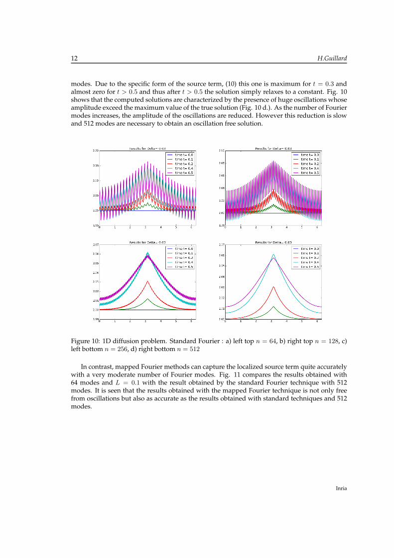
In contrast, mapped Fourier methods can capture the localized source term quite accuratelywith a very moderate number of Fourier modes. Fig. 11 compares the results obtained with64 modes and L = 0.1 with the result obtained by the standard Fourier technique with 512modes. It is seen that the results obtained with the mapped Fourier technique is not only freefrom oscillations but also as accurate as the results obtained with standard techniques and 512modes.

Inria

Mapped Fourier Methods in toroidal geometry 13

Figure 11: 1D diffusion problem Mapped Fourier (MF) compared to standard method : a) leftStandard Fourier with 512 modes, b) right MF using 64 modes and L = 0.1

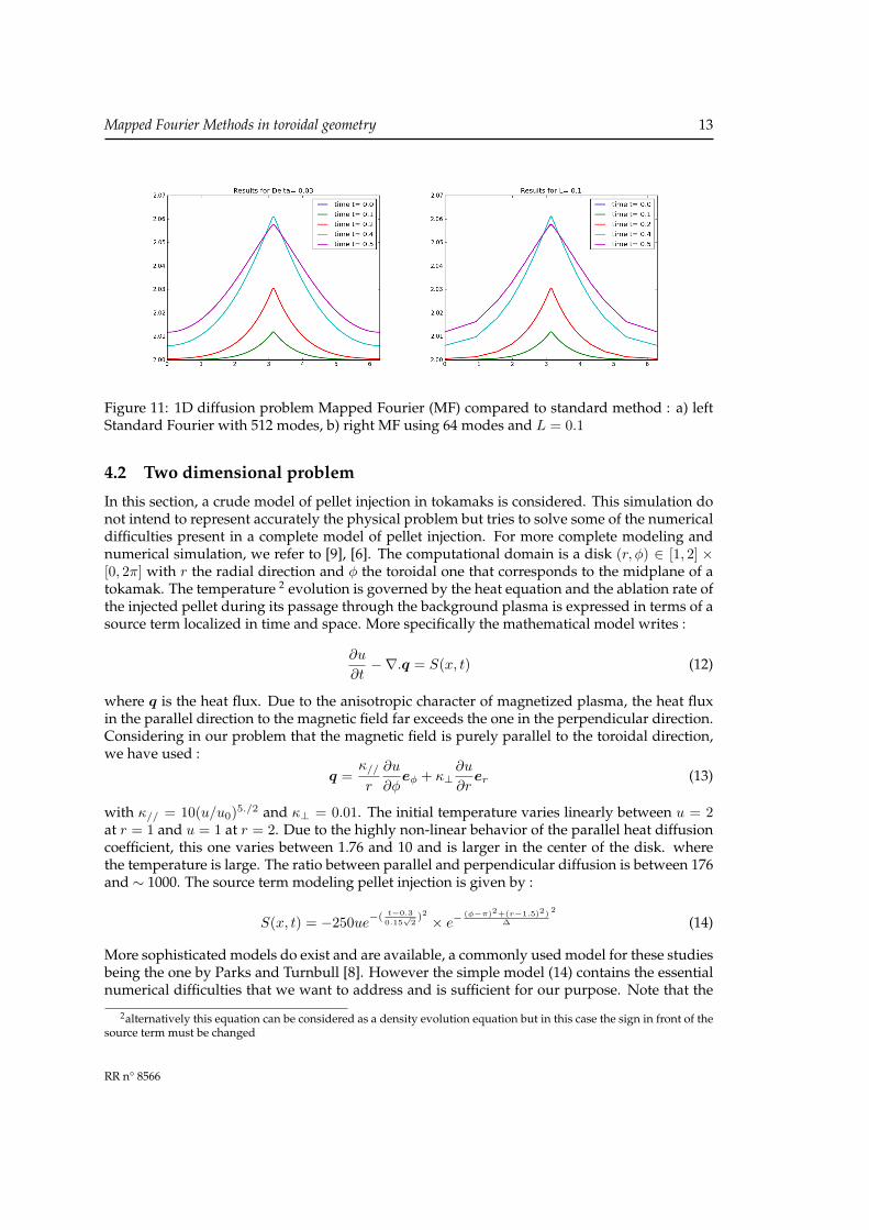
4.2 Two dimensional problem

In this section, a crude model of pellet injection in tokamaks is considered. This simulation donot intend to represent accurately the physical problem but tries to solve some of the numericaldifficulties present in a complete model of pellet injection. For more complete modeling andnumerical simulation, we refer to [9], [6]. The computational domain is a disk (r, φ) ∈ [1, 2] ×[0, 2π] with r the radial direction and φ the toroidal one that corresponds to the midplane of atokamak. The temperature 2 evolution is governed by the heat equation and the ablation rate ofthe injected pellet during its passage through the background plasma is expressed in terms of asource term localized in time and space. More specifically the mathematical model writes :

∂u

∂t−∇.q = S(x, t) (12)

where q is the heat flux. Due to the anisotropic character of magnetized plasma, the heat fluxin the parallel direction to the magnetic field far exceeds the one in the perpendicular direction.Considering in our problem that the magnetic field is purely parallel to the toroidal direction,we have used :

q =κ//

r

∂u

∂φeφ + κ⊥

∂u

∂rer (13)

with κ// = 10(u/u0)5./2 and κ⊥ = 0.01. The initial temperature varies linearly between u = 2at r = 1 and u = 1 at r = 2. Due to the highly non-linear behavior of the parallel heat diffusioncoefficient, this one varies between 1.76 and 10 and is larger in the center of the disk. wherethe temperature is large. The ratio between parallel and perpendicular diffusion is between 176and ∼ 1000. The source term modeling pellet injection is given by :

S(x, t) = −250ue−( t−0.30.15√

2)2 × e−

(φ−π)2+(r−1.5)2)∆

2

(14)

More sophisticated models do exist and are available, a commonly used model for these studiesbeing the one by Parks and Turnbull [8]. However the simple model (14) contains the essentialnumerical difficulties that we want to address and is sufficient for our purpose. Note that the

2alternatively this equation can be considered as a density evolution equation but in this case the sign in front of thesource term must be changed

RR n° 8566

14 H.Guillard

source term is negative as the injection of cryogenic pellets in a very hot plasma gives rise toa local drop of the plasma temperature. The parameter ∆ is related to the pellet radius thatis by several orders of magnitude smaller than the tokamak size. In this work, we have taken∆ = 0.03. A mapped Fourier method has been used in the toroidal direction and a simple finitedifference one in the radial direction. Fig 12 presents the distribution of collocations points inthe computational domain. The right plot shows that the points are highly concentrated at thelocation of the source.

Figure 12: Left : Distribution of collocation points in the physical space, Right : Zoom on thesource region

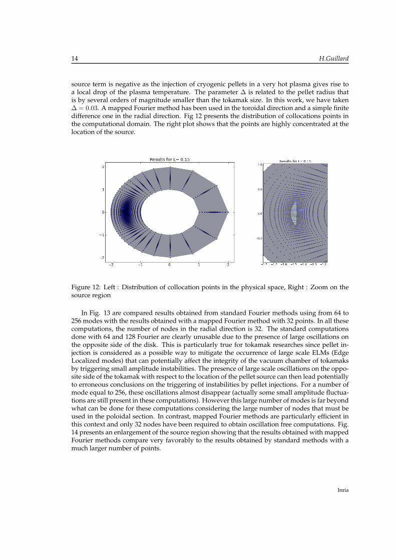
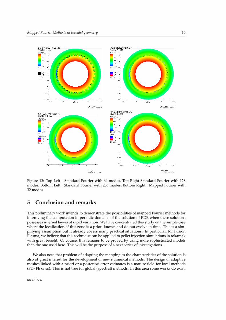
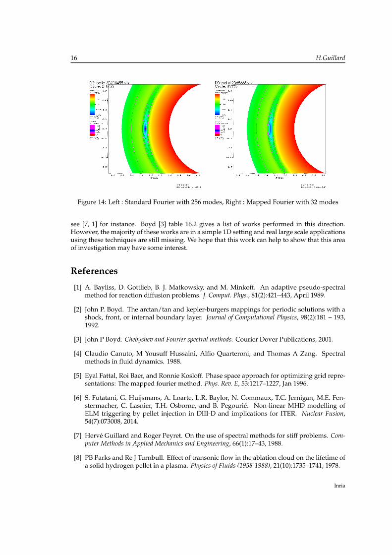
In Fig. 13 are compared results obtained from standard Fourier methods using from 64 to256 modes with the results obtained with a mapped Fourier method with 32 points. In all thesecomputations, the number of nodes in the radial direction is 32. The standard computationsdone with 64 and 128 Fourier are clearly unusable due to the presence of large oscillations onthe opposite side of the disk. This is particularly true for tokamak researches since pellet in-jection is considered as a possible way to mitigate the occurrence of large scale ELMs (EdgeLocalized modes) that can potentially affect the integrity of the vacuum chamber of tokamaksby triggering small amplitude instabilities. The presence of large scale oscillations on the oppo-site side of the tokamak with respect to the location of the pellet source can then lead potentiallyto erroneous conclusions on the triggering of instabilities by pellet injections. For a number ofmode equal to 256, these oscillations almost disappear (actually some small amplitude fluctua-tions are still present in these computations). However this large number of modes is far beyondwhat can be done for these computations considering the large number of nodes that must beused in the poloidal section. In contrast, mapped Fourier methods are particularly efficient inthis context and only 32 nodes have been required to obtain oscillation free computations. Fig.14 presents an enlargement of the source region showing that the results obtained with mappedFourier methods compare very favorably to the results obtained by standard methods with amuch larger number of points.

Inria

Mapped Fourier Methods in toroidal geometry 15

Figure 13: Top Left : Standard Fourier with 64 modes, Top Right Standard Fourier with 128modes, Bottom Left : Standard Fourier with 256 modes, Bottom Right : Mapped Fourier with32 modes

5 Conclusion and remarks

This preliminary work intends to demonstrate the possibilities of mapped Fourier methods forimproving the computation in periodic domains of the solution of PDE when these solutionspossesses internal layers of rapid variation. We have concentrated this study on the simple casewhere the localization of this zone is a priori known and do not evolve in time. This is a sim-plifying assumption but it already covers many practical situations. In particular, for FusionPlasma, we believe that this technique can be applied to pellet injection simulations in tokamakwith great benefit. Of course, this remains to be proved by using more sophisticated modelsthan the one used here. This will be the purpose of a next series of investigations.

We also note that problem of adapting the mapping to the characteristics of the solution isalso of great interest for the development of new numerical methods. The design of adaptivemeshes linked with a priori or a posteriori error estimates is a mature field for local methods(FD/FE ones). This is not true for global (spectral) methods. In this area some works do exist,

RR n° 8566

16 H.Guillard

Figure 14: Left : Standard Fourier with 256 modes, Right : Mapped Fourier with 32 modes

see [7, 1] for instance. Boyd [3] table 16.2 gives a list of works performed in this direction.However, the majority of these works are in a simple 1D setting and real large scale applicationsusing these techniques are still missing. We hope that this work can help to show that this areaof investigation may have some interest.

References

[1] A. Bayliss, D. Gottlieb, B. J. Matkowsky, and M. Minkoff. An adaptive pseudo-spectralmethod for reaction diffusion problems. J. Comput. Phys., 81(2):421–443, April 1989.

[2] John P. Boyd. The arctan/tan and kepler-burgers mappings for periodic solutions with ashock, front, or internal boundary layer. Journal of Computational Physics, 98(2):181 – 193,1992.

[3] John P Boyd. Chebyshev and Fourier spectral methods. Courier Dover Publications, 2001.

[4] Claudio Canuto, M Yousuff Hussaini, Alfio Quarteroni, and Thomas A Zang. Spectralmethods in fluid dynamics. 1988.

[5] Eyal Fattal, Roi Baer, and Ronnie Kosloff. Phase space approach for optimizing grid repre-sentations: The mapped fourier method. Phys. Rev. E, 53:1217–1227, Jan 1996.

[6] S. Futatani, G. Huijsmans, A. Loarte, L.R. Baylor, N. Commaux, T.C. Jernigan, M.E. Fen-stermacher, C. Lasnier, T.H. Osborne, and B. Pegourié. Non-linear MHD modelling ofELM triggering by pellet injection in DIII-D and implications for ITER. Nuclear Fusion,54(7):073008, 2014.

[7] Hervé Guillard and Roger Peyret. On the use of spectral methods for stiff problems. Com-puter Methods in Applied Mechanics and Engineering, 66(1):17–43, 1988.

[8] PB Parks and Re J Turnbull. Effect of transonic flow in the ablation cloud on the lifetime ofa solid hydrogen pellet in a plasma. Physics of Fluids (1958-1988), 21(10):1735–1741, 1978.

Inria

Mapped Fourier Methods in toroidal geometry 17

[9] R Samtaney, SC Jardin, Phillip Colella, and Daniel F Martin. 3d adaptive mesh refinementsimulations of pellet injection in tokamaks. Computer physics communications, 164(1):220–228, 2004.

[10] Jie Shen and Li-Lian Wang. Error analysis for mapped legendre spectral and pseudospec-tral methods. SIAM J. Numer. Anal, 42:326–349, 2004.

[11] Jie Shen and Li-Lian Wang. Error analysis for mapped jacobi spectral methods. J. Sci.Comput., 24:183–218, 2005.

RR n° 8566

RESEARCH CENTRESOPHIA ANTIPOLIS – MÉDITERRANÉE

2004 route des Lucioles - BP 9306902 Sophia Antipolis Cedex

PublisherInriaDomaine de Voluceau - RocquencourtBP 105 - 78153 Le Chesnay Cedexinria.fr

ISSN 0249-6399