RICE UNIVERSITY

MAP Detection with Soft Information in an

Estimate and Forward Relay Network

by

Corina Ioana Serediuc

A Thesis Submittedin Partial Fulfillment of theRequirements for the Degree

Master of Science

Approved, Thesis Committee:

Dr. Behnaam Aazhang, ChairJ.S. Abercrombie Professor of Electricaland Computer Engineering

Dr. Edward W. KnightlyProfessor of Electrical and ComputerEngineering

Dr. Jorma LillebergAdjunct Professor in Electrical andComputer Engineering

Dr. Ashutosh SabharwalAssociate Professor of Electrical andComputer Engineering

Houston, Texas

April, 2011

ii

ABSTRACT

MAP Detection with Soft Information in an Estimate-and-Forward Relay Network

by Corina Ioana Serediuc

One proven solution for improving the reliability of a wireless channel is to use

relays. In this thesis, we analyse the three-node relay network, which is the funda-

mental scheme in cooperative communications. A relay protocol is defined by the way

the received signal (relay function) is processed at the relay. Our main focus is on the

estimate-and-forward (EF) relay protocol, where the relay node estimates the source

symbol and then forwards it to the destination. The type of information sent by the

relay is the defining element of a relay protocol, and it is known as soft information

in the EF protocol.

We assume that the soft information sent by the relay is the minimum mean square

error (MMSE) estimate for the conditional expectation of the symbol transmitted by

the source. For the case of BPSK modulation in a pathloss model for the cooperative

three-node wireless network, we show that EF outperforms other common relay pro-

tocols such as amplify-and-forward (AF) and detect-and-forward (DF). The detection

at the destination uses the optimal maximum a posteriori (MAP) detector. Since the

probability density function (pdf) required by this detector does not have an ana-

lytical form, we provide a solution to bypass its numerical approximation, needed

at the MAP detector. A piecewise linear approximation of the MMSE estimate is

used as soft information. The linearity conserves the Gaussian properties of the sent

information and thus the pdf of the received signal at the destination from the source

has a straightforward analytical form. This approximation provides a closed form

expression for the detector and its performance is similar to the case when a MMSE

estimate is used.

Contents

List of Illustrations v

1 Introduction 1

1.1 Relaying strategies . . . . . . . . . . . . . . . . . . . . . . . . . . . . 3

1.2 Main contribution of this thesis . . . . . . . . . . . . . . . . . . . . . 4

2 Related work 6

3 Preliminaries 11

3.1 System model . . . . . . . . . . . . . . . . . . . . . . . . . . . . . . . 11

3.2 Detector at destination . . . . . . . . . . . . . . . . . . . . . . . . . . 14

3.2.1 Proof of independence . . . . . . . . . . . . . . . . . . . . . . 16

3.3 Decode-and-Forward . . . . . . . . . . . . . . . . . . . . . . . . . . . 17

3.4 Amplify-and-Forward . . . . . . . . . . . . . . . . . . . . . . . . . . . 19

4 Estimate and Forward 22

4.1 Relay function . . . . . . . . . . . . . . . . . . . . . . . . . . . . . . . 23

4.1.1 BSPK modulation . . . . . . . . . . . . . . . . . . . . . . . . 24

4.1.2 M-QAM modulation . . . . . . . . . . . . . . . . . . . . . . . 26

4.2 Detector at the destination . . . . . . . . . . . . . . . . . . . . . . . . 28

4.2.1 Pdf of the MMSE estimate . . . . . . . . . . . . . . . . . . . . 29

4.3 Piecewise linear approximation . . . . . . . . . . . . . . . . . . . . . 32

5 Simulation results 37

iv

6 Conclusions 42

A 43

Appendix A 43

Bibliography 46

Illustrations

1.1 Wireless cooperative network setup. . . . . . . . . . . . . . . . . . . . 2

1.2 Three-node relay network. . . . . . . . . . . . . . . . . . . . . . . . . 3

2.1 Three node cooperative wireless network . . . . . . . . . . . . . . . . 7

3.1 Three-node wireless network. . . . . . . . . . . . . . . . . . . . . . . . 11

3.2 Pathloss model. Relay inline with source and destination. . . . . . . . 13

3.3 Transmission protocol. First time slot - Broadcast phase; Second time

slot - MAC phase - usually both the source and the relay transmit in

this phase, but in our case, only the relay will be transmitting. . . . . 13

3.4 Relay functions for AF and DF; ySR is the received signal at the relay

and f(ySR) is the relay function. For this plot, we have considered

BPSK modulation, SNRSR = 3dB and an average transmit power

constraint at the relay PR = 1. . . . . . . . . . . . . . . . . . . . . . 20

4.1 Relay functions for AF, DF and EF; ySR is the received signal at the

relay and f(ySR) is the relay function. For this plot, we have

considered BPSK modulation, SNRSR = 3dB and an average

transmit power constraint at the relay PR = 1. . . . . . . . . . . . . 24

4.2 The relay function fEF (ySR) plotted for different values of SNRSR

from −1dB to 20dB. . . . . . . . . . . . . . . . . . . . . . . . . . . . 25

vi

4.3 Relay functions for AF, DF and EF; ySR is the received signal at the

relay and f(ySR) is the relay function. For this plot we have

considered 4PAM modulation. The pathloss model is considered with

d = 0.7 and α = 4. . . . . . . . . . . . . . . . . . . . . . . . . . . . . 28

4.4 Probability density function of E[x|ySR] for x = 1, for different values

of SNRSR. . . . . . . . . . . . . . . . . . . . . . . . . . . . . . . . . . 30

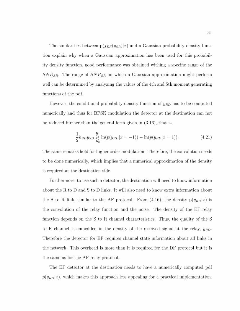
4.5 Relay functions for EF with MMSE estimate and EF with linear

approximation; ySR is the received signal at the relay and f(ySR) is

the relay function. For this plot, we have considered BPSK

modulation, SNRSR = 3dB and an average transmit power

constraint at the relay PR = 1. . . . . . . . . . . . . . . . . . . . . . . 33

4.6 Relay functions for AF, DF, EF with MMSE and EF - linear; ySR is

the received signal at the relay and f(ySR) is the relay function. For

this plot, we have considered BPSK modulation, SNRSR = 3dB and

an average transmit power constraint at the relay PR = 1. . . . . . . 34

5.1 Pdf p(yRD|x = 1) for the EF relay protocol with the MMSE estimate.

The density is shown for different positions of the relay with respect

to the source (different d). . . . . . . . . . . . . . . . . . . . . . . . 38

5.2 BER for AF, DF and EF protocols for BPSK modulation for the

pathloss model. On the x-axis, d represents the normalized distance

between S and R. . . . . . . . . . . . . . . . . . . . . . . . . . . . . 39

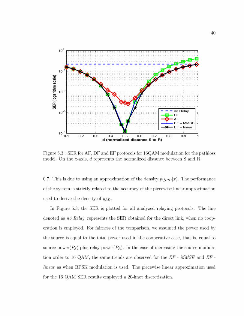
5.3 SER for AF, DF and EF protocols for 16QAM modulation for the

pathloss model. On the x-axis, d represents the normalized distance

between S and R. . . . . . . . . . . . . . . . . . . . . . . . . . . . . 40

1

Chapter 1

Introduction

In recent years, wireless communications have evolved tremendously. One important

difference from wired communications is that in the wireless environment the com-

munication medium is shared among users. Thus, other nodes in the neighbourhood

of the transmitting node are able to hear the transmission. Due to the availability

of information at nodes in the vicinity of the source, the idea of using these nodes

to help with communication emerged. This technique became known as cooperative

communications. The information at the receiving node depends not only on the sig-

nal received from the source, but also on the signals received from neighbouring nodes.

This thesis analyses the type of information the neighbouring nodes should send to

aid the communication and provides a strategy for the best use of the additional

information at the destination node.

The maximum amount of information that can be sent over the shared medium

in a wireless network is constrained by the interference among nodes. For long dis-

tance communications, the transmitted signal suffers attenuation and also produces

interference to more nodes in the system. In contrast, short distance communications

produce interference to a smaller number of neighbours, allowing more communica-

tion channels to be active in the wireless network. This advantage of short distance

wireless communications motivated the use of multihop networks. In such a network,

nodes pass information to the next ones, until the data reaches its destination node.

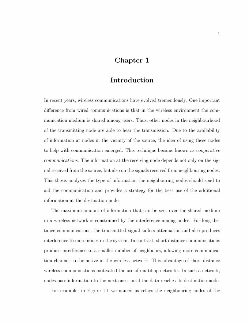
For example, in Figure 1.1 we named as relays the neighbouring nodes of the

2

Figure 1.1 : Wireless cooperative network setup.

source which can hear the full transmission. When the source transmits, the relays

can help communication in several ways. One possible multihop link can be formed

with relays 2 and 3 by sending the signal from one to the another until it reaches

the destination. Also, a one-hop link can be formed with relay 1, which retransmits

the signal directly to the destination. Thus, if the direct communication between

the source and the destination is weak, then the destination can combine the signal

received from the source with the signals received from relays 1 and 3 to correctly

decode the information.

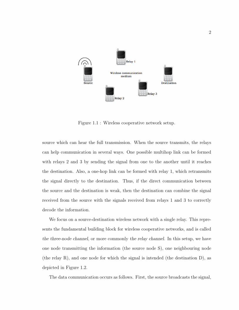
We focus on a source-destination wireless network with a single relay. This repre-

sents the fundamental building block for wireless cooperative networks, and is called

the three-node channel, or more commonly the relay channel. In this setup, we have

one node transmitting the information (the source node S), one neighbouring node

(the relay R), and one node for which the signal is intended (the destination D), as

depicted in Figure 1.2.

The data communication occurs as follows. First, the source broadcasts the signal,

3

Figure 1.2 : Three-node relay network.

which is heard by both the relay and the destination. Secondly, the relay processes

its received signal and forwards it to the destination. During this time, the source

may be silent, such that only the relay transmits, or it may also broadcast new data.

This forces the relay to perform in full duplex mode, receiving and transmitting

at the same time. The importance of cooperative communications becomes clear

when information is retrieved at the destination. In a point-to-point network (no

relays), when the source-destination link is bad, the information may not be decoded

accurately. However, in a cooperative setting, the destination can use additional

information from the relays, resulting in an improved decoding.

One major factor which influences the accuracy of the decoding performed at the

destination is the type of information sent by the relay. Next, we present several well

known relaying strategies which use different types of information forwarding by the

relay.

1.1 Relaying strategies

A relay protocol is defined by the type of processing used for the received signal at

the relay. There are three main classes of relaying protocols:

• Decode-and-Forward (DF). The relay decodes and re-encodes the received

4

signal, then it forwards it to the destination. This processing of the signal at

the relay is also know as making a hard decision, as the information sent by the

relay does not include any additional information about the reliability of the

source-relay link.

• Amplify-and-Forward (AF). In this case, the relay just amplifies its received

signal, maintaining a fixed average transmit power.

• Estimate-and-Forward(EF). This protocol is also known as Compress-and-

Forward or Quantize-and-Forward. At the relay, a transformation is applied

to the received signal, which provides an estimate of the source signal. This

estimate is called soft information, and it is forwarded to the destination.

AF is a straightforward scheme for both coded and uncoded systems. On the

other hand, DF comes with the option of choosing a specific type of coding which can

improve the overall performance. Both protocols have been extensively investigated

using capacity, achievable rates and also different metrics such as outage probability,

bit-error-rate (BER) or throughput. These two schemes present a complementary

behavior which depends on the signal to noise ratio regimes.

1.2 Main contribution of this thesis

While AF and DF have well defined signal processing at the relay, the EF relay

protocol includes a broad variety of estimates which can be sent to the destination

to improve detection. Thus, since EF is not restricted to only one type of processing

at the relay, it has raised a lot of interest on what should be the best estimate to

use, or how should this estimate best be used at the destination. In this work, we

5

address these questions and show how EF can be used to improve the performance

of the system over AF and DF.

Previous work on EF has shown that there are optimal estimates which minimize

specific performance criteria. Motivated by this, we represent the soft information at

the relay by the minimum mean squared error(MMSE) estimate. We show that EF

with the MMSE estimate provides superior performance to both AF and DF, with

respect to bit-error-rate(BER). We propose using a piecewise linear approximation of

the MMSE estimate to obtain a closed form detector at the destination.

6

Chapter 2

Related work

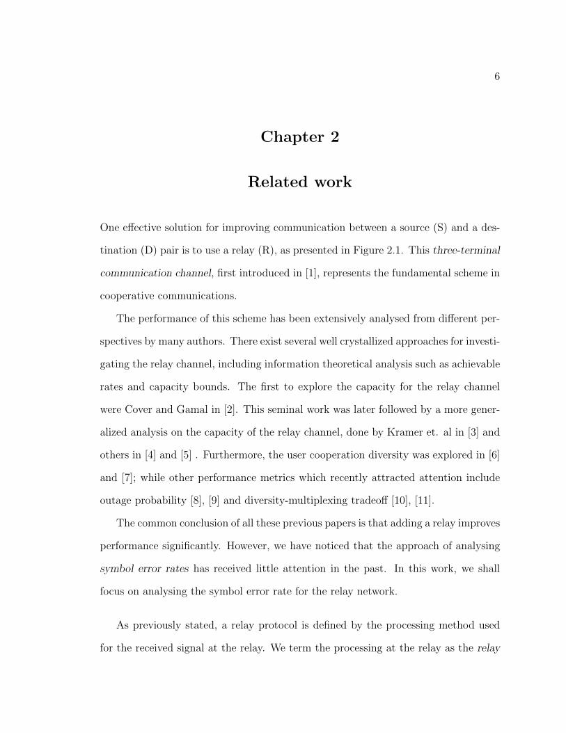
One effective solution for improving communication between a source (S) and a des-

tination (D) pair is to use a relay (R), as presented in Figure 2.1. This three-terminal

communication channel, first introduced in [1], represents the fundamental scheme in

cooperative communications.

The performance of this scheme has been extensively analysed from different per-

spectives by many authors. There exist several well crystallized approaches for investi-

gating the relay channel, including information theoretical analysis such as achievable

rates and capacity bounds. The first to explore the capacity for the relay channel

were Cover and Gamal in [2]. This seminal work was later followed by a more gener-

alized analysis on the capacity of the relay channel, done by Kramer et. al in [3] and

others in [4] and [5] . Furthermore, the user cooperation diversity was explored in [6]

and [7]; while other performance metrics which recently attracted attention include

outage probability [8], [9] and diversity-multiplexing tradeoff [10], [11].

The common conclusion of all these previous papers is that adding a relay improves

performance significantly. However, we have noticed that the approach of analysing

symbol error rates has received little attention in the past. In this work, we shall

focus on analysing the symbol error rate for the relay network.

As previously stated, a relay protocol is defined by the processing method used

for the received signal at the relay. We term the processing at the relay as the relay

7

Figure 2.1 : Three node cooperative wireless network

function f(ySR), where ySR denotes the received signal at the relay.

Two basic relay protocols were first proposed by Cover and El Gamal in [2].

These protocols are decode-and-forward (DF) and compress-and-forward (CF) also

known as estimate-and-forward (EF). Another important protocol, called amplify-

and-forward (AF) has been well investigated by Laneman in [9, 8, 12] and others

[13, 14, 15]. Furthermore, other protocols can be derived from these basic ones, such

as quantized-and-forward (QF) [16].

One of the main features of the AF and DF protocols is that the relay function is

well defined. Thus, a lot of attention has been directed towards these protocols, see

[3]-[15]. On the other hand, the analysis of the EF protocol can prove to be rather

tedious, since the EF relay function is defined to be any type of estimate of the source

signal which could aid the detection at the destination. As a result, among the three

most prominent relaying protocols, EF has received the least attention in literature.

When investigating the EF protocol, besides the metric used to showcase the re-

sults, there are several characteristics which make each analysis unique. They include

the network topology, the relay function, and the criterion on which the EF relay func-

tion is chosen. Another important aspect of EF is the type of information each node

8

is required to have. In addition, most of the existing EF work completely ignores the

direct link between the source and the destination, and little to no attention has been

given to the detector at the destination side.

For the two-hop transmission network topology, pioneering contributions in EF

relaying were made by Abou-Faycal and Medard in [17], where they focused on obtain-

ing the relay function which minimizes the probability of error. A network topology

similar to the one in Fig.2.1 was considered, but with no direct link from S to D.

Channel state information was assumed to be known at each receiver (CSIR at R and

D) and in addition to the R to D channel, the S to R channel state was assumed to be

known at the receiver D. With these assumptions, the optimal relay function which

minimizes the probability of error was found to be the Lambert W, which is defined

as the solution to W(x)eW(x) = x. The results were derived for uncoded antipodal

signalling in conjunction with an additive white Gaussian noise (AWGN) assumption

on each of the two channels. This function is non-analytical and requires analytical

approximation or table look up. Therefore, the detector at the destination is not

tractable.

Using a similar setup, Gomadam and Jafar proved in [18] that forwarding the

minimum mean squared error (MMSE) estimate maximizes the generalized signal to

noise ratio (SNR) at the destination. The network topology was extended to ones

involving multiple relays in a parallel and serial topology arrangements. These results

were derived for the relaying network without exploiting the direct link between S

and D. In addition, in [19], the same authors showed numerically that the MMSE

estimate is capacity optimal for BPSK modulation in a two hop relay network.

The work presented [17] was later extended by Cui et. al [20] for the two way

relay channel. For binary antipodal signalling, in a network which included the direct

9

link, they showed that a Lambert W function minimizes the probability of error.

The Lambert W function and the MMSE estimate are the only EF relay functions

to optimize a criterion such as the probability of error or SNR. These functions are

specific for the uncoded system for the relay network. For a coded relay network,

the functions encountered in literature are approximations of the mean squared error

(MSE) estimate as the log likelihood functions (LLRs) [21, 22] or approximations

of the LLRs, [23]. However, our focus in this paper shall be solely on an uncoded

system, which uses the MMSE estimate as the relay function.

In previous work on EF, the relay function depends only on the received symbol

and not on previous symbols. This methodology was recently denoted as instanta-

neous relaying by Khormuji in [24], where they performed analysis for the Gaussian

relay channel with a direct link and a perfect S to R link. Khormuji and Skoglund

numerically showed that a relay protocol with parametric piecewise linear mapping

improves the performance of the relay network over the AF relay protocol. In this

paper we propose a more generalized method which employs a piecewise linear ap-

proximation of the relay function.

Once the relay function is defined for a relay protocol, the detector at the destina-

tion is critical for the practical implementation of the protocol. In the communications

literature, sparse attention has been given to the detector techniques which could be

used at the destination. Seminal work was done by Brennan in [33], where a compre-

hensive analysis is done on the practical maximum-ratio-combining (MRC) detector

applied to both AF and DF. Later, Wang et. al [25] introduced cooperative-MRC

(C-MRC) and showed that for a DF relay protocol maximum possible diversity is

achieved. Most recently, a novel soft-symbol estimate-and-forward (SEF) with the

MRC detector technique is proposed by Hu and Lilleberg in [26]. They show numer-

10

ically that significant power gain is obtained when a posteriori probability is used to

weight the soft information sent by the relay.

We argue that in a wireless environment, the direct link may still provide reliable

information and warrant processing at the destination. The MMSE estimate has

been shown to be optimum in several scenarios of the three-node network without

the direct link. Thus, in this work we analyse the performance of the EF protocol

when a conditional expectation is the relay function in a three-node wireless network,

and we take advantage of the existence of the direct link. We provide a generalized

method consisting of using a piecewise linear approximation of the MMSE. We also

address the important issue of the detection algorithm at the destination. To the

best of our knowledge, we are among the first to provide a closed form solution of the

optimal detector.

It has also come to our attention that recently, similar work has been done in-

dependently and in parallel by Tian et al in [27]. They use a specific three-segment

piecewise linear approximation in a system with BPSK modulation.

11

Chapter 3

Preliminaries

In this chapter, we define the system model and two of the most well know protocols,

amplify-and-forward (AF) and decode-and-forward (DF). Their performance will later

be compared with the performance of the proposed EF protocol.

3.1 System model

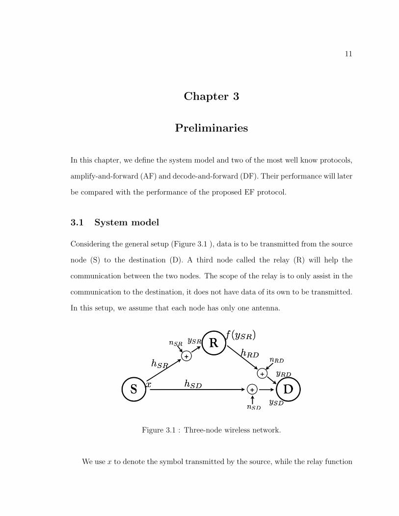
Considering the general setup (Figure 3.1 ), data is to be transmitted from the source

node (S) to the destination (D). A third node called the relay (R) will help the

communication between the two nodes. The scope of the relay is to only assist in the

communication to the destination, it does not have data of its own to be transmitted.

In this setup, we assume that each node has only one antenna.

Figure 3.1 : Three-node wireless network.

We use x to denote the symbol transmitted by the source, while the relay function

12

is represented by f(ySR), where ySR denotes the received signal at the relay from the

source. Similarly, we define yRD and ySD as the received signals at the destination.

According to the type of function used at the relay, we can classify the the signal

transmitted by the relay as soft or hard information. Results presented throughout

this thesis will be given for the general case with fading channels, and specific examples

will be shown for different modulation schemes. The fading coefficient of S-R, R-D

and S-D channels are denoted by hSR, hRD and hSD, respectively. Every channel in

the network is degraded by independent AWGN as nSR ∼ N (0, 1), nSD ∼ N (0, 1)

and nRD ∼ N (0, 1). It follows that the system model is described by the following

equations:

ySR = hSR · x+ nSR (3.1)

ySD = hSD · x+ nSD (3.2)

yRD = hRD · f(ySR) + nRD (3.3)

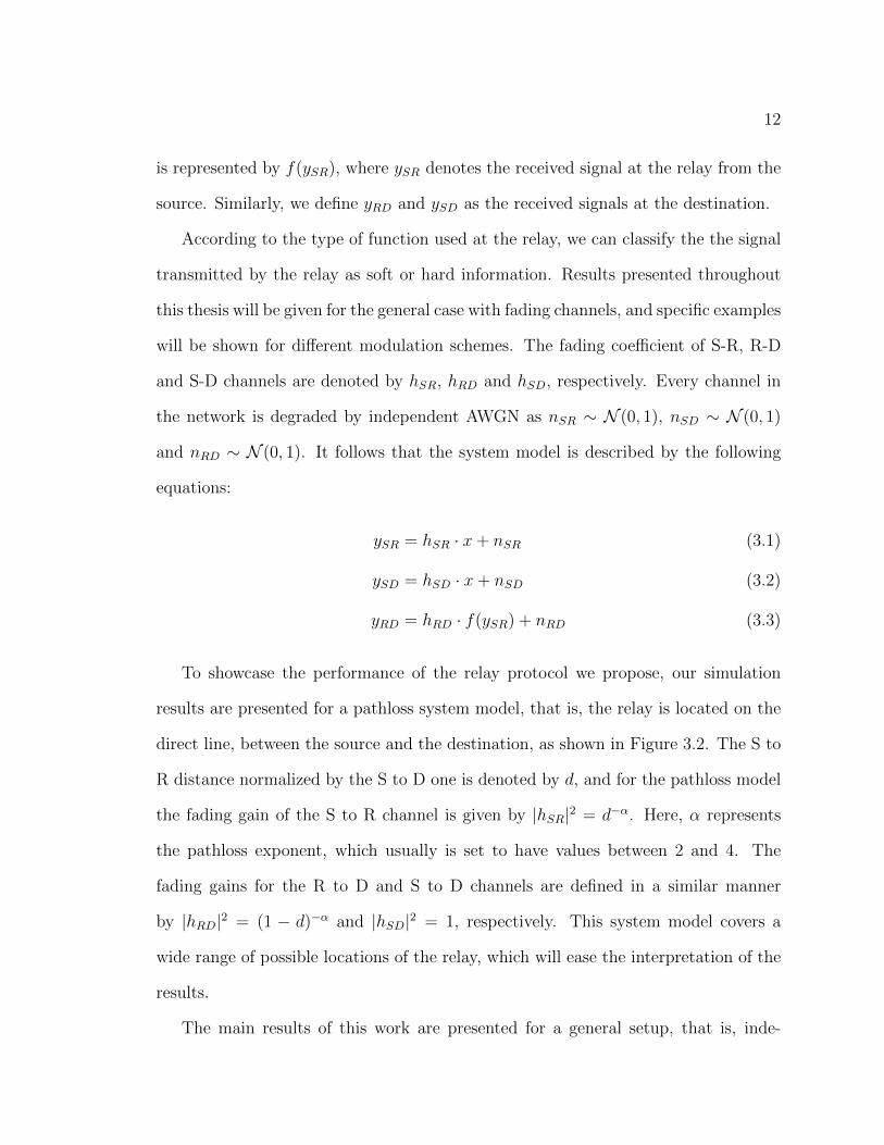
To showcase the performance of the relay protocol we propose, our simulation

results are presented for a pathloss system model, that is, the relay is located on the

direct line, between the source and the destination, as shown in Figure 3.2. The S to

R distance normalized by the S to D one is denoted by d, and for the pathloss model

the fading gain of the S to R channel is given by |hSR|2 = d−α. Here, α represents

the pathloss exponent, which usually is set to have values between 2 and 4. The

fading gains for the R to D and S to D channels are defined in a similar manner

by |hRD|2 = (1 − d)−α and |hSD|2 = 1, respectively. This system model covers a

wide range of possible locations of the relay, which will ease the interpretation of the

results.

The main results of this work are presented for a general setup, that is, inde-

13

Figure 3.2 : Pathloss model. Relay inline with source and destination.

pendent of the modulation order chosen for the source symbols. Examples are given

for specific modulations like uncoded binary-phase-shift-keying (BPSK) and M-ary

QAM (quadrature amplitude modulation), such as 16 QAM. We assume fixed trans-

mit power for the source (PS) and the relay (PR). Their sum is equal to the source

transmit power in a S to D only model, that is, the single link model with no relays.

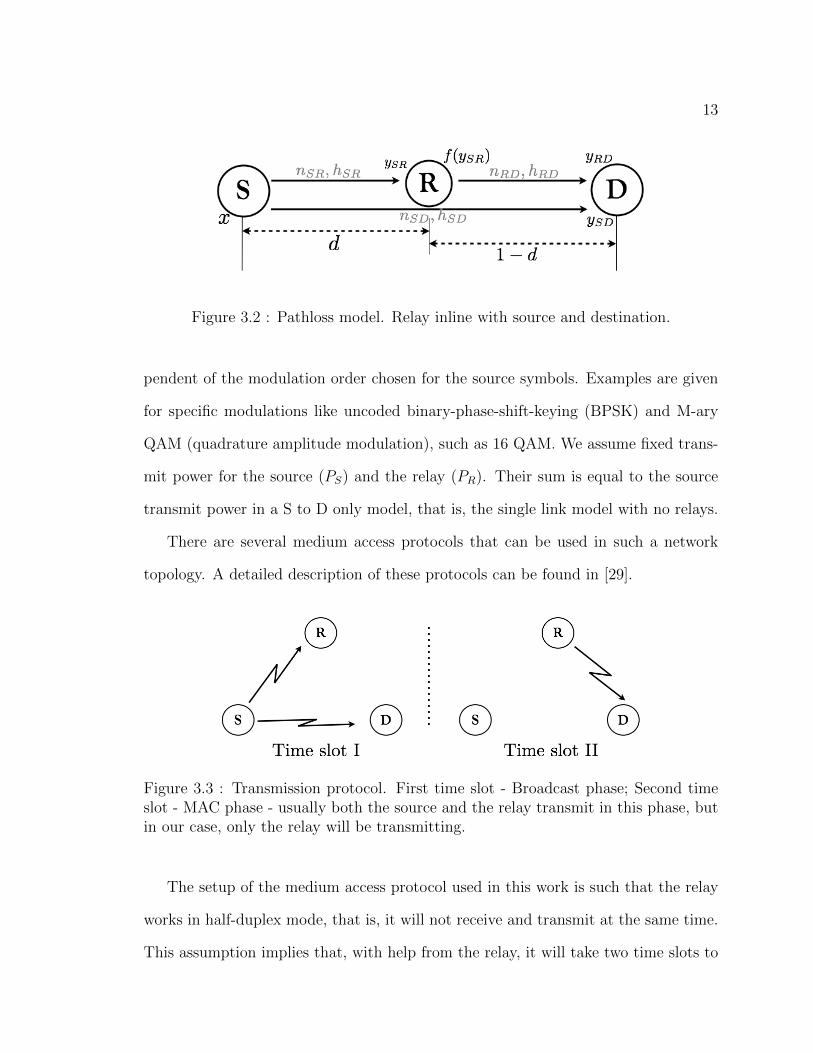
There are several medium access protocols that can be used in such a network

topology. A detailed description of these protocols can be found in [29].

Figure 3.3 : Transmission protocol. First time slot - Broadcast phase; Second timeslot - MAC phase - usually both the source and the relay transmit in this phase, butin our case, only the relay will be transmitting.

The setup of the medium access protocol used in this work is such that the relay

works in half-duplex mode, that is, it will not receive and transmit at the same time.

This assumption implies that, with help from the relay, it will take two time slots to

14

complete the transmission from S to D, as shown in Figure 3.3. In the first time slot,

also know as the broadcast phase, S transmits, while R is silent and both R and D

receive the signal. In the second time slot, S is silent and only R transmits to D.

We also impose the CSIR assumption, that is, channel state information is known

at the receiver. This a realistic assumption, since training pilots can be used to

estimate the channel characteristics and frequency offset correction can be applied at

the receiver to recover from constellation rotation.

An important aspect of any relaying protocol is the detector at the destination.

The decision at the destination is done based on all received signals, ySD and yRD.

In the next section we introduce the optimal detector to be used at the destination.

3.2 Detector at destination

Once the two signals ySD, yRD are received at D, the optimal detector is used in the

form of a maximum a posteriori probability (MAP) detector. The MAP detector is

given by,

xD = maxx

pX|YSDYRD(x|ySD, yRD) (3.4)

where xD denotes the symbol resulted from the decision made at the destination

side. From now on we drop the subscripts, which are obvious by inspection of the

arguments of the probability density function. The subscripts will be shown only in

those cases when they are essential for clarity.

Applying Bayes’ Rule[30] we obtain.

xD = maxx

p(ySD, yRD|x)p(x)

p(ySD, yRD). (3.5)

The decision at the destination is made for given values of ySD and yRD, thus the

term p(ySD, yRD) is constant for any given value of x. We can ignore this term, as it

15

is independent of x and it does not affect the end result of the detector. We assume

the symbols are equally likely, therefore p(x) has the same value for any given symbol

and thus it does not influence the outcome of the detector. With these assumptions,

the general form of the detector can be further simplified as

xD = maxx

p(ySD, yRD|x) (3.6)

= maxx

p(ySD|x)p(yRD|x). (3.7)

The detector given in (3.6) is the well known maximum likelihood (ML) detector.

The MAP and ML detector are the same for this system, mainly because equally

likely symbols are used for transmission.

The transition from (3.6) to (3.7) is possible because of the following system

properties. The first is that the noise is i.i.d. on all channels, due to the nature of

the wireless communication medium. Combining this property with the fact that the

two probability density functions are conditioned on x, we get that the two random

variables representing the received signals at the destination, ySD and yRD given x

are independent.

The proof for the conditional independence of the two variables is independent on

the modulation order and it is given in the following subsection. Thus, the form of

the detector given in (3.7) is specific to this model setup of the network and it will

be used throughout the rest of this work and exemplified for specific modulations.

16

3.2.1 Proof of independence

Applying Bayes’ rule on the two variables ySD and yRD from the detector given in

(3.5) we obtain:

xD = maxx

p(ySD, yRD|x) = (3.8)

= maxx

p(yRD|ySD, x)p(ySD|x) (3.9)

= maxx

p(yRD|x)p(ySD|x), (3.10)

where going from 3.9 to 3.10 is possible due to the following result:

p(yRD|x, ySD) = p(hRDf(ySR) + nRD|x, hSDx+ nSD) (3.11)

= p(hRDf(hSRx+ nSR) + nRD|x, hSDx+ nSD) (3.12)

= p(hRDf(hSRx+ nSR) + nRD|x) (3.13)

= p(ySD|x). (3.14)

In (3.12), we expand the received signals ySD and ySR according to the system model

given in (3.1)-(3.3). The noise on each channel is independent, thus nSD is inde-

pendent of nRD and nSR. Therefore in (3.13) conditioning on nSD gives the same

probability value as not conditioning on it. In the last step (3.14), we return to the

compact form of ySD given in (3.2).

For example, for BPSK modulation the detector given in (3.7) becomes a simple

comparison between two probability values

p(yRD|x = 1)p(ySD|x = 1)H1

≷H0

p(yRD|x = 1)p(ySD|x = 1) (3.15)

where the hypotheses H0 and H1 are given by H0 = {x = −1} and H1 = {x = 1}.

Given the system model in (3.2) and the channel and noise characteristics, we can

17

apply the natural logarithm in 3.15 and simplify to get

1

2hSDySD

H1

≷H0

ln(p(yRD|x = −1))− ln(p(yRD|x = 1)). (3.16)

As each relay protocol depends on the specificity of the relay function, this influ-

ences the form of the probability density function (pdf) p(yRD|x). The density of the

received signal at the destination from the source ySD is not affected by the change

in the relay function. Thus, the conditional probability density function of yRD plays

an important role in defining the decision rule at the destination.

For 16 QAM, the detector in (3.7) can be reduced to having several comparisons

between the 16 possible symbols, similar in form to the ones for BPSK, (3.15).

Now that the detector under study has been identified we will turn our attention

to the relay function. Next, we introduce the most common relaying protocols by

investigating the associated relay functions. The relay function is the defining element

of a relay protocol and the system performance is directly affected by the “quality”

of the signal received at the relay. Throughout this thesis we investigate three forms

of relaying and we consider their symbol error performance.

3.3 Decode-and-Forward

In the DF protocol the relay decodes the received signal, re-encodes it and then

forwards it to the destination. This type of signal processing is also known as making

a hard decision at the relay

fDF (ySR) = x (3.17)

where x represents the decoded symbol at the relay. For the case when uncoded

signals are considered, the protocol is known as detect-and-forward.

18

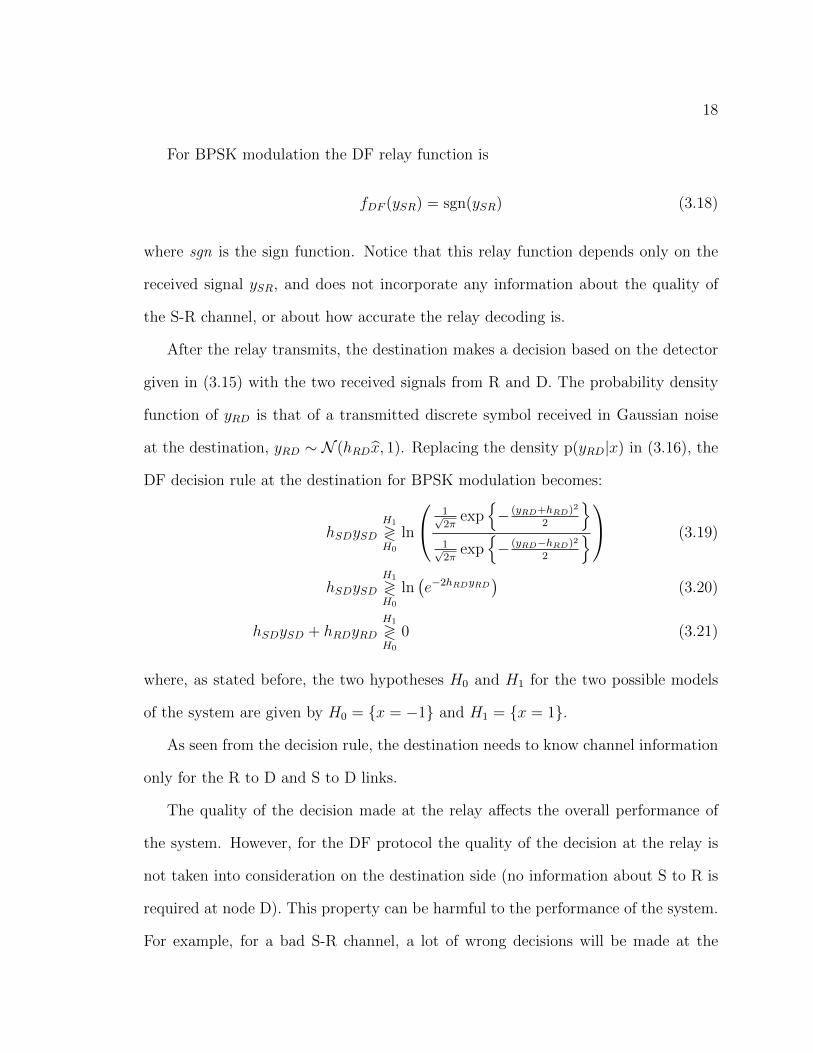
For BPSK modulation the DF relay function is

fDF (ySR) = sgn(ySR) (3.18)

where sgn is the sign function. Notice that this relay function depends only on the

received signal ySR, and does not incorporate any information about the quality of

the S-R channel, or about how accurate the relay decoding is.

After the relay transmits, the destination makes a decision based on the detector

given in (3.15) with the two received signals from R and D. The probability density

function of yRD is that of a transmitted discrete symbol received in Gaussian noise

at the destination, yRD ∼ N (hRDx, 1). Replacing the density p(yRD|x) in (3.16), the

DF decision rule at the destination for BPSK modulation becomes:

hSDySDH1

≷H0

ln

1√2π

exp{− (yRD+hRD)2

2

}1√2π

exp{− (yRD−hRD)2

2

} (3.19)

hSDySDH1

≷H0

ln(e−2hRDyRD

)(3.20)

hSDySD + hRDyRDH1

≷H0

0 (3.21)

where, as stated before, the two hypotheses H0 and H1 for the two possible models

of the system are given by H0 = {x = −1} and H1 = {x = 1}.

As seen from the decision rule, the destination needs to know channel information

only for the R to D and S to D links.

The quality of the decision made at the relay affects the overall performance of

the system. However, for the DF protocol the quality of the decision at the relay is

not taken into consideration on the destination side (no information about S to R is

required at node D). This property can be harmful to the performance of the system.

For example, for a bad S-R channel, a lot of wrong decisions will be made at the

19

relay. Even if the R-D channel is very good, the destination will not be able tell the

accuracy of the signal sent by the relay, fDF (ySR). On the other hand, suppose the

S-R channel is good and assume that symbol 1 was sent. If a weak signal is received

at the relay, for example ySR = 0.1, when it is forwarded to the destination it will be

amplified to the symbol power PR · 1. This means a correct decision has been made

and a strong signal has been sent for this decision.

These are some of the most important advantages and disadvantages of DF. We

will later see that EF with MMSE estimate incorporates most of the advantages of

DF.

3.4 Amplify-and-Forward

The AF relay function is an amplification of the received signal,

fAF (ySR) = βySR (3.22)

with β the relay transmit average power constraint coefficient. The coefficient β

ensures that the average transmit power at the relay is constant and equal to PR,

therefore β is derived in a similar way to the one obtained by Laneman in [9]:

E[|f(ySR)|2] ≤ PR (3.23)

E[|βySR|2] ≤ PR (3.24)

β2E[|hSRx+ nSR|2] ≤ PR (3.25)

β ≤

√PR

h2SRE[|x|2] + E[|nSR|2](3.26)

and for Gaussian noise with unit variance and Es, the energy of the symbol becomes

β ≤

√PR

h2SREs+ 1. (3.27)

20

−2 −1.5 −1 −0.5 0 0.5 1 1.5 2−2

−1.5

−1

−0.5

0

0.5

1

1.5

2

ySR

f(y

SR

)

Relay function

DF

AF

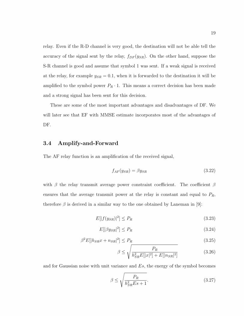
Figure 3.4 : Relay functions for AF and DF; ySR is the received signal at the relayand f(ySR) is the relay function. For this plot, we have considered BPSK modulation,SNRSR = 3dB and an average transmit power constraint at the relay PR = 1.

The form of the AF relay function given in (3.22) is independent of the modulation

scheme of the source symbol. Since the transmitted signal at the relay is linear in ySR,

as seen in Figure 3.4, for higher values of ySR the relay requires more instantaneous

transmit power than the case when the DF relay function is used.

The probability density function of ySD is the same as in the DF relaying protocol,

while the signal yRD is

yRD = hRDβySR + nRD = hRDβ(hSRx+ nSR) + nRD

= βhSRhRDx+ hRDβnSR + nRD. (3.28)

Therefore, given the independence of the noise and using the linear property of Gaus-

sian random variables, the conditional probability density function of yRD is

p(yRD|x) = N (βhSRhRDx, h2RDβ

2 + 1). (3.29)

This probability density function together with the one for ySD, are replaced in the

detector given in (3.7) and a simplified formulation is obtained. Note, that until now,

all the results shown for AF are independent on the modulation order.

21

For example, for BPSK modulation, replacing 3.29 in the detector form given in

(3.16), we get that the detector at the destination is given by

hSDySDH1

≷H0

ln

1√2π(h2RDβ

2+1)exp

{− (yRD+βhSRhRD)2

2h2RDβ2+1

}1√

2π(h2RDβ2+1)

exp{− (yRD−βhSRhRD)2

2(h2RDβ2+1)

} (3.30)

hSDySDH1

≷H0

ln

(exp

{−4βhSRhRDyRD

2(h2RDβ2 + 1)

})(3.31)

hSDySD +βhSRhRDh2RDβ

2 + 1yRD

H1

≷H0

0. (3.32)

In addition to the DF decision rule, for which the destination is required to know

only S to D and R to D link characteristics, AF requires extra information about

the S to R link. This implies that for the AF relay protocol the destination decision

rule takes into consideration the quality of the channel between S and R. Therefore,

one might assume that AF should perform better than the DF protocol. However,

we show in the simulation results that this is not always true; the performance of

different relay protocols is directly influenced by the quality of the channels, and

more precisely by the position of the relay. One argument for this behavior is that,

for the AF protocol, when the relay amplifies the received signal it also amplifies the

noise. For very good channel conditions, the DF protocol makes the right decision,

eliminating the noise, while the AF relay protocol, amplifies the noise. Thus, for high

SNR on the S to R channel, a clean signal as the one provided by the DF protocol is

prefered at the destination, rather than the noisy signal resulted from the AF relay

function.

In the next chapter we introduce the EF relay protocol and its characteristics for

specific relay functions.

22

Chapter 4

Estimate and Forward

The class of estimate-and-forward relay protocols includes any “useful” side informa-

tion which the relay can provide to the destination in support of its detection and

decoding of the information from the source. The EF relay function is often referred

to as soft information.

There are many other types of “side” information that the relay can forward to

destination to help with decoding. For example, any type of signal estimate is a

possible soft information. From the broad range of possible relay functions, only few

improve the overall performance of EF. In [17], Abou-Faycal and Medard showed

that the Lambert W function minimizes the probability of error in a system without

the direct link. Others, such as Gomadam and Jafar, proved that the MMSE max-

imizes the receiver SNR and numerically showed that it is capacity optimal, again

for a system without the direct link, [18]. These two functions are very similar in

form. Log-likelihood ratio (LLR) functions have also been used as soft information,

as an approximation of the MMSE estimate, but proved to encounter difficulties at

the detector located at destination, [21]. Hu and Lilleberg in [26] used a weighted

type of soft information which mimics the behavior of the MMSE estimate. In this

work, we use the MMSE estimate as the relay function because of the properties

this transformation has, and because it efficiently incorporates information about the

quality of the S to R channel.

The next section introduces the MMSE estimate as a relay function and presents

23

the properties which give intuition on the expected behavior of the EF relay protocol.

4.1 Relay function

We assume the relay function for the EF protocol is the MMSE estimate, which is

the conditional expectation of the source sent symbol x given the received signal at

the relay ySR

fEF (ySR) = kE[x|ySR] = k∑x

xp(x|ySR). (4.1)

After applying Bayes’ rule, we get

fEF (ySR) = k∑x

xp(ySR|x)p(x)

p(ySR)= k

∑x

xp(ySR|x)p(x)∑x

p(ySR|x)p(x), (4.2)

where k is the average transmit power constraint coefficient for the relay. Therefore,

for an average transmit power at the relay PR we can obtain the value of k similarto

the AF case:

E[|k ∗ E[x|ySR]|2] ≤ PR (4.3)

k ≤

√PR

E[|E[x|ySR]|2](4.4)

where | · | represents the absolute value.

Next, we investigate its characteristics by applying it to different modulation

schemes and by comparing it to the common relay functions presented so far. The

conditional density function of ySR given the source symbol x is the same as for the DF

and AF relay protocols, that is p(ySR|x) = N (hSRx, 1). Introducing the conditional

probability density function of ySR in (4.2), the EF relay function is further expanded

24

as

fEF (ySR) = k

∑x

xN (hSRx, 1)p(x)∑x

N (hSRx, 1)p(x)(4.5)

= k

∑x

x 1√2π

exp{− (y−hSRx)

2

2

}p(x)∑

x

1√2π

exp{− (y−hSRx)2

2

}p(x)

. (4.6)

4.1.1 BSPK modulation

When the source uses antipodal signals, x ∈ {−1, 1}, also known as BPSK modula-

tion, the soft information of the EF protocol shown in (4.6) becomes

fEF (ySR) = kehSRySR − e−hSRySR

ehSRySR + e−hSRySR= k tanh (ySRhSR) . (4.7)

−2 −1.5 −1 −0.5 0 0.5 1 1.5 2−2

−1.5

−1

−0.5

0

0.5

1

1.5

2

ySR

f(y

SR

)

Relay function

DF

AF

ideal EF

Figure 4.1 : Relay functions for AF, DF and EF; ySR is the received signal at the relayand f(ySR) is the relay function. For this plot, we have considered BPSK modulation,SNRSR = 3dB and an average transmit power constraint at the relay PR = 1.

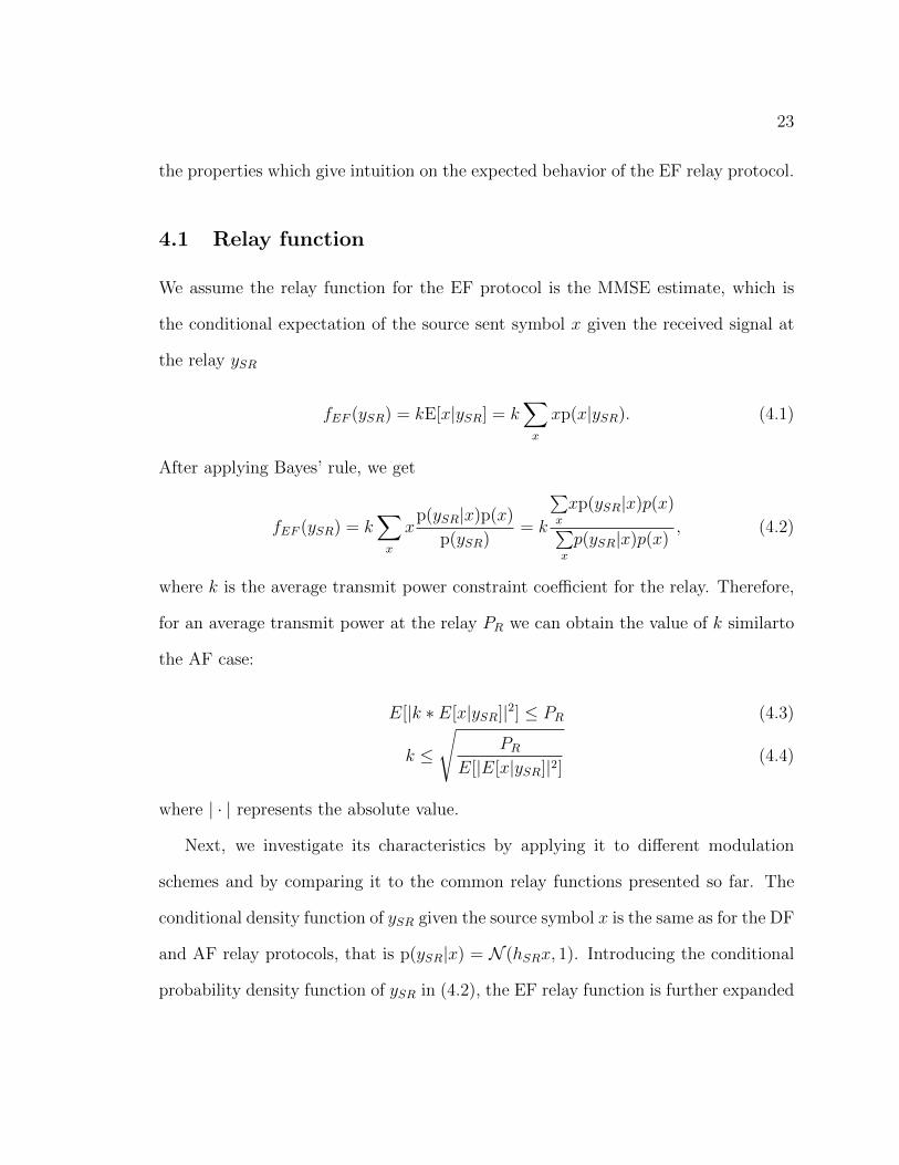
The EF relay function specific for BPSK modulation is shown in Figure 4.1, where

both the AF and DF relay functions are also plotted. The MMSE as the EF relay

25

function is denoted as ideal EF. One important observation made on this graph is

that the EF relay function is inbetween the AF and DF ones. This attracted our

attention on the specific form of the MMSE estimate.

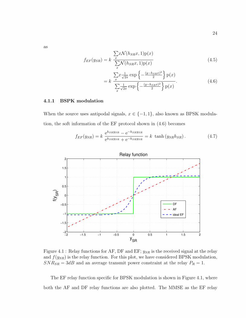
We noticed that the quality of the S to R link has great influence on the perfor-

mance of the EF protocol, as seen in Figure 4.2. We define SNR to represent signal

to noise ratio at the receiver. For high values of the SNRSR, when the relay is closer

to the source, the MMSE estimate becomes very steep and similar to the DF hard

decision relay function. While, for low values of the SNRSR (the relay is closer to the

−2 −1.5 −1 −0.5 0 0.5 1 1.5 2−1.5

−1

−0.5

0

0.5

1

1.5

ySR

f EF(y

SR)

SNRSR

= −1dB

SNRSR

= 1dB

SNRSR

= 20dB

Figure 4.2 : The relay function fEF (ySR) plotted for different values of SNRSR from−1dB to 20dB.

destination), the EF relay function is similar to the AF one. Thus, we expect that

for high SNR on the S to R link, EF will perform as good as DF and for a degraded

S to R channel, the performance of the system will be similar to AF.

With this type of soft information, we expect the EF relay protocol to perform

as the best of AF and DF. Furthermore, the MMSE estimate inherits one important

26

property from the DF protocol: the instantaneous transmit power at the relay is

slightly higher than for DF, but it is much lower than the one the AF protocol

requires. This can be observed in Figure 4.1; for ySR ≥ 1.3 the AF relay protocol

requires more instantaneous transmit power than all other schemes.

4.1.2 M-QAM modulation

A variety of communications protocols implement quadrature amplitude modulation

(QAM), for example current protocols such as 802.11b wireless Ethernet (Wi-Fi) and

digital video broadcast (DVB) use 64-QAM modulation. Next, we present the general

EF relay function from (4.2) for the case when QAM modulation is used for the source

symbol x. Specific examples are given for rectangular QAM, such as 16-QAM.

Rectangular QAM is considered when the amplitudes of the carriers are a set of

discrete values. This is equivalent to having two orthonormal signals represented with

pulse-amplitude modulation (PAM) for the real and imaginary parts of the source

transmitted signal. Such representations imply that the real and imaginary parts can

be considered as two independent signals. As a result, the relay function applies to

each part individually and independently

fEF (ySR) = kE[x|ySR] (4.8)

= k(E[Re(x)|Re(ySR)] + iE[Im(x)|Im(ySR)]) (4.9)

= k(fEF/RePAM(Re(ySR)) + ifEF/ImPAM(Im(ySR))

)(4.10)

where fEF/RePAM(Re(ySR)) and fEF/ImPAM(Im(ySR)) are the notations for the EF

relay function applied to the real and imaginary part representation of the sent signal

x given the real and imaginary part representation of the received signal at the relay,

ySR.

27

We introduce the EF relay function for the real part, which means fEF is applied

to PAM modulation. The imaginary part is treated in a similar way. The probability

density function of the real part of the received signal at the relay is the same as in

the AF and DF relay protocols, that is, N (hSRRe(x), 1). Applying it to the EF relay

function given in (4.2), it becomes

fEF (Re(ySR)) = k

∑Re(x)

Re(x)p(Re(ySR)|Re(x))p(Re(x))∑Re(x)

p(Re(ySR)|Re(x))p(Re(x))(4.11)

= k

∑x

xN (hSRx, 1)p(x)∑x

N (hSRx, 1)p(x)(4.12)

= k

∑x

x 1√2π

exp{− (y−hSRx)

2

2

}p(x)∑

x

1√2π

exp{− (y−hSRx)2

2

}p(x)

(4.13)

where in (4.12) and (4.13) we dropped the Re() notation for clarity, such that x

denotes Re(x) and ySR denotes Re(ySR). For 16QAM modulation, 4PAM modu-

lation is used for each of the rectangular coordinates which are also known as the

In-phase (I) and Quadrature (Q) coordinates of the signal. Applying 4PAM modula-

tion to each coordinate implies that Re(x) ∈ {−3,−1, 1, 3}, and similarly for Im(x).

Expanding the relay function given in (4.13) for the 4PAM modulation, we obtain

the relay function specific for each coordinate that preserves the estimate-and-forward

characteristics:

f4PAM(y) =∑x

xp(y|x)p(x)

p(y)(4.14)

=−3e−6hSRy−9h2SR − e−2hSRy−h2SR + e2hy−h

2+ 3e6hSRy−9h2SR

e−6hSRy−9h2SR + e−2hSRy−h2SR + e2hSRy+h2SR + e6hSRy−9h2SR

(4.15)

where y represents either the imaginary or real part of ySR, and x the equivalent part

for source sent symbol.

28

−10 −8 −6 −4 −2 0 2 4 6 8 10

−4

−3

−2

−1

0

1

2

3

4

ySR

f(y

SR

)

Relay function for 4PAM modulation

DF

AF

EF − MMSE

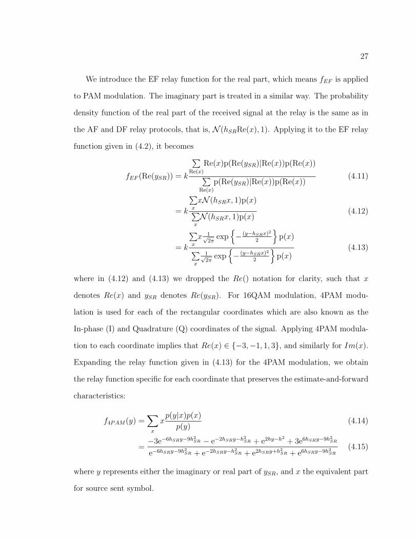
Figure 4.3 : Relay functions for AF, DF and EF; ySR is the received signal at the relayand f(ySR) is the relay function. For this plot we have considered 4PAM modulation.The pathloss model is considered with d = 0.7 and α = 4.

As it can be seen in Figure 4.3, the MMSE estimate for 4PAM modulation has the

same characteristics as for BPSK modulation, in comparison with the relay functions

for AF and DF. Therefore, we showed that using higher order modulation for the

source symbol x maintains the MMSE estimate properties.

Next, we turn our attention to the detector at the destination and its character-

istics.

4.2 Detector at the destination

As stated previously, the detector is the same for all cases analyzed. Therefore,

the general form of the MAP detector for the EF protocol is independent on the

modulation of the source signal and it is given in (3.7), with its specific form for BPSK

shown in (3.16). The detector at the destination requires the density p(ySD|x), which

29

is the same for all three relaying protocols analyzed. The conditional probability

density function of yRD is dependent on the specificity of the relay function and

introduces differences in the destination detector.

For the EF relaying protocol, as a result of (3.3), one way to obtain p(yRD|x) is

through the convolution of the probability density function of the relay function and

the Gaussian density of the noise, as shown bellow

p(yRD|x) = p(fEF (ySR)|x) ∗ p(nRD|x). (4.16)

Once the two densities are defined, a decision rule can be implemented at the desti-

nation following the form of the MAP detector given in (3.7). However, there is no

analytical form for the conditional probability density function of yRD and therefore

no analytical form for the detector at the destination. Next, we analyze the proba-

bility density function of the MMSE estimate to gain insight into its characteristics.

4.2.1 Pdf of the MMSE estimate

One can obtain the probability density function of the signal sent by the relay,

p(fEF (ySR)|x), using the formula for the density of a function of a random vari-

able shown in equation 4.18 (also see chapter x from [30]). Using this method, the

conditional probability density function of the conditional expectation is derived.

For example, for BPSK modulation with the notation

z = E[x|ySR] = f(ySR) ⇒ ySR = f−1(z) (4.17)

we derive

pZ|X(z|x) = pYSR|X(f−1(z)|x) · (f−1)′(z) (4.18)

= pYSR|X

(1

2hSRln

(1 + z

1− z

)∣∣∣∣x) 1

hSR

1

1− z2. (4.19)

30

Now, pZ|X(z|x) is defined in terms of the probability density function of ySR, which

is know. Therefore, we obtain the following closed form for the conditional pdf of the

MMSE estimate for BPSK modulation

pZ|X(z|x) =1

hSR(1− z2)1√2π

exp

{−1

2

[1

2hSRln

(1 + z

1− z

)− hSRx

]2}(4.20)

where, as denoted in (4.17), z = E[x|ySR].

The probability density function given in (4.20) has finite support and is presented

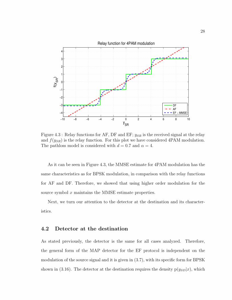
in Figure 4.4, where we have only shown the corresponding pdf for x = 1, as the pdf

of E[x|ySR] for x = −1 is symmetric with respect to the y-axis. Notice that for lower

SNR values of the S - R channel, the probability density function has a Gaussian

form, but as SNRSR increases, the Gaussian similarities disappear.

−1 −0.8 −0.6 −0.4 −0.2 0 0.2 0.4 0.6 0.8 10

1

2

3

4

5

6

7

8

9

x 10−4

E[x|ySR

]

p(E

[x|y

SR]|x

=1)

Density function of E[x|ySR

] for x = 1

SNRSR

= −20 dB

SNRSR

= −15 dB

SNRSR

= −10 dB

SNRSR

= −5 dB

SNRSR

= −1 dB

SNRSR

= 5 dB

SNRSR

= 5 dB

SNRSR

= −5 dB

SNRSR

= −10 dB

SNRSR

= −20 dB

Figure 4.4 : Probability density function of E[x|ySR] for x = 1, for different values ofSNRSR.

Using a similar approach, the probability density function of the MMSE estimate

for higher order modulation can be obtained.

31

The similarities between p(fEF (ySR)|x) and a Gaussian probability density func-

tion explain why when a Gaussian approximation has been used for this probabil-

ity density function, good performance was obtained withing a specific range of the

SNRSR. The range of SNRSR on which a Gaussian approximation might perform

well can be determined by analyzing the values of the 4th and 5th moment generating

functions of the pdf.

However, the conditional probability density function of yRD has to be computed

numerically and thus for BPSK modulation the detector at the destination can not

be reduced further than the general form given in (3.16), that is,

1

2hSDySD

H1

≷H0

ln(p(yRD|x = −1))− ln(p(yRD|x = 1)). (4.21)

The same remarks hold for higher order modulation. Therefore, the convolution needs

to be done numerically, which implies that a numerical approximation of the density

is required at the destination side.

Furthermore, to use such a detector, the destination will need to know information

about the R to D and S to D links. It will also need to know extra information about

the S to R link, similar to the AF protocol. From (4.16), the density p(yRD|x) is

the convolution of the relay function and the noise. The density of the EF relay

function depends on the S to R channel characteristics. Thus, the quality of the S

to R channel is embedded in the density of the received signal at the relay, yRD.

Therefore the detector for EF requires channel state information about all links in

the network. This overhead is more than it is required for the DF protocol but it is

the same as for the AF relay protocol.

The EF detector at the destination needs to have a numerically computed pdf

p(yRD|x), which makes this approach less appealing for a practical implementation.

32

Therefore, in the following, we propose a solution to bypass the need of a numerical

probability density function.

4.3 Piecewise linear approximation

The solution we propose for overcoming the need of a numerical density function

is to use a piecewise linear approximation of the conditional expectation. The soft

information sent by the relay is composed of multiple linear functions, defined as:

flin(ySR) = k ·

a1ySR + b1, ySR ∈ (−∞, y1)

a2ySR + b2, ySR ∈ (y1, y2)

· · ·

aiySR + bi, ySR ∈ (yi−1, yi)

· · ·

an+1ySR + bn+1, ySR ∈ (yn,+∞)

(4.22)

where k is the transmit power constraint coefficient

k ≤√

PR

E[|flin(ySR)|2

] . (4.23)

For i ∈ (2, n + 1), the coefficients ai and bi are dependent on yi−1, yi, fEF (yi−1)

and fEF (yi) as follows:

ai =fEF (yi)− fEF (yi−1)

yi − yi−1(4.24)

bi =fEF (yi−1)yi − fEF (yi)yi−1

yi − yi−1. (4.25)

In (4.22), (4.24) and (4.25), the points yi−1 and yi belong to the set of n points

{y1 < y2 < · · · < yn} on the real line, called knots (see [32], lecture 11). The knots

are chosen to minimize the L1 norm, which is equivalent to minimizing the area

33

−1.5 −1 −0.5 0 0.5 1 1.5

−1

−0.5

0

0.5

1

ySR

f(y

SR

)

Relay function

ideal EF

linear EF

soft information (ideal EF)

y3

y4

linear aproximation(linear EF)

y1

y2

Figure 4.5 : Relay functions for EF with MMSE estimate and EF with linear ap-proximation; ySR is the received signal at the relay and f(ySR) is the relay function.For this plot, we have considered BPSK modulation, SNRSR = 3dB and an averagetransmit power constraint at the relay PR = 1.

between the two relay functions:

minset{yi}i=1...n

∫ +∞

−∞|fEF (ySR)− flin(ySR)| dySR (4.26)

The accuracy of the approximation depends on the number of knots chosen. For

example, for BPSK modulation, the relay function flin(ySR) is shown in Figure 4.5,

for a four-knot (or five-segment) approximation.

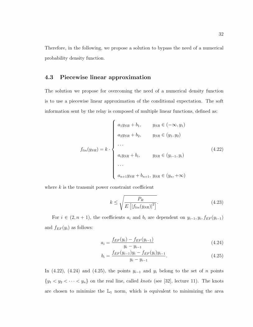
The same function can be compared with the corresponding functions for AF

and DF, see Figure 4.6. Since it is a good approximation of the MMSE estimate,

we expect the behavior of the system to be similar. Compared to the conditional

expectation, this relay function requires less resources at the relay, as it is just a

linear transformation of the received signal.

Due to the linearity of the approximation, the relay function maintains the Gaus-

34

−2 −1.5 −1 −0.5 0 0.5 1 1.5 2−2

−1.5

−1

−0.5

0

0.5

1

1.5

2

ySR

f(y S

R)

Relay function

DF

AF

ideal EF

linear EF

AF

hard information(DF)

soft information (ideal EF)

linear aproximation(linear EF)

Figure 4.6 : Relay functions for AF, DF, EF with MMSE and EF - linear; ySR isthe received signal at the relay and f(ySR) is the relay function. For this plot, wehave considered BPSK modulation, SNRSR = 3dB and an average transmit powerconstraint at the relay PR = 1.

sian property of ySR. The received symbol at the destination becomes:

yRD = (4.27)

hRDk(a1ySR + b1) + nRD, ySR ∈ (−∞, y1)

· · ·

hRDk(aiySR + bi) + nRD, ySR ∈ (yi−1, yi)

· · ·

hRDk(an+1ySR + bn+1) + nRD, ySR ∈ (yn,+∞)

with i ∈ (2 . . . n). Since the system uses instantaneous relaying and the relay function

flin(ySR) is deterministic, the density p(yRD|x) is given by:

p(yRD|x) =

∫ +∞

−∞p(yRD|ySR)p(ySR|x)dySR. (4.28)

The signal yRD has specific forms for different regions with respect to ySR, as seen in

35

(4.27). This imposes a similar form for the density of yRD given that ySR is known.

When the noise is AWGN this density is:

p(yRD|ySR) =

N (m1, 1), ySR ∈ (−∞, y1)

· · ·

N (mi, 1), ySR ∈ (yi−1, yi)

· · ·

N (mn+1, 1), ySR ∈ (yn,+∞)

(4.29)

where the means of the Gaussian densities mi are given by:

mi = hRDk(aiySR + bi). (4.30)

In (4.28), we substitute both the density p(yRD|ySR) given in (4.29) and the prob-

ability density function p(ySR|x) given by N (hSRx, 1). We can now compute the

analytical form of the density p(yRD|x). After simplifying and rearranging the vari-

ables (intermediate steps are shown in Appendix A), the probability of the signal sent

from the relay and received at the destination becomes

p(yRD | x) =

=1√

2πσ2rd(1)

exp

{−(yRD −mrd(1)

)22σ2

rd(1)

}Q

(−y1 −msr(1)

σsr(1)

)(4.31)

+n∑i=2

1√2πσ2

rd(i)

exp

{−(yRD −mrd(i)

)22σ2

rd(i)

}[Q

(yi−1 −msr(i)

σsr(i)

)−Q(yi −msr(i)

σsr(i)

)]

+1√

2πσ2rd(n+1)

exp

{−(yRD −mrd(n+1)

)22σ2

rd(n+1)

}Q

(yn −msr(n+1)

σsr(n+1)

)

where the means msr(i) and mrd(i) and variances σ2sr(i) and σ2

rd(i) depend on the cor-

36

responding intervals through ai and bi as shown bellow:

msr(i) =hRDkai(yRD − hRDkbi) + hSRx

1 + h2RDk2a2i

(4.32)

σ2sr(i) =

1

1 + h2RDk2a2i

(4.33)

mrd(i) = hRDk(bi + hSRxai) (4.34)

σ2rd(i) = 1 + h2RDk

2a2i . (4.35)

In previous notations we used the subscript rd(i) to denote that the mean/variance

which pertains to a Gaussian density function of the random variable indicated by the

subscript, in this case that is yRD. Also, the subscript (i) denotes that the notation

is dependent on the interval (yi−1, yi). Furthermore, the form of the conditional pdf

given in (4.31) can be interpreted as a sum of the probability of yRD being received

at the destination, given that the signal sent by the relay is in a specific region

(ySR ∈ (yi−1, yi)), scaled by the probability of being in that interval. The destination

will need to be synchronized with the relay such that it will know exactly what knots

are chosen for the approximation.

The detector for the EF protocol shown in (4.21) has analytical form and can be

implemented using the density of the piecewise linear approximation given in (4.31).

A higher performance requirement implies the need for a better approximation,

which can be obtained using a higher number of knots. However, a higher number

of knots increases the complexity of the density and thus of the detector at the

destination. Depending on the system requirements, there will always be a trade-off

between the complexity of the detector and the accuracy of the approximation.

37

Chapter 5

Simulation results

In this chapter, we evaluate the proposed relay protocol for the three-node network

with the pathloss system model described in Chapter 3. We use the Symbol-error-rate

(SER) as the metric to evaluate the performance of each relaying protocol.

Simulation results for the EF protocol with MMSE estimate were possible as the

probability density function p(yRD|x) was evaluated numerically. Although this pdf

does not have an analytical form, using Monte Carlo simulations we obtained a good

numerical approximation of it. The numerical form of this density gave us further

insight into the influence of the MMSE estimate on the performance of the EF relaying

protocol.

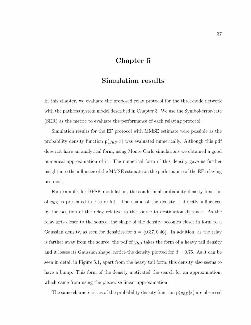
For example, for BPSK modulation, the conditional probability density function

of yRD is presented in Figure 5.1. The shape of the density is directly influenced

by the position of the relay relative to the source to destination distance. As the

relay gets closer to the source, the shape of the density becomes closer in form to a

Gaussian density, as seen for densities for d = {0.37, 0.46}. In addition, as the relay

is farther away from the source, the pdf of yRD takes the form of a heavy tail density

and it losses its Gaussian shape; notice the density plotted for d = 0.75. As it can be

seen in detail in Figure 5.1, apart from the heavy tail form, this density also seems to

have a bump. This form of the density motivated the search for an approximation,

which came from using the piecewise linear approximation.

The same characteristics of the probability density function p(yRD|x) are observed

38

Figure 5.1 : Pdf p(yRD|x = 1) for the EF relay protocol with the MMSE estimate.The density is shown for different positions of the relay with respect to the source(different d).

for the case when the source modulation is increased to 16 QAM.

When the source uses BPSK modulation the symbol-error-rate (SER) is the same

as the bit-error-rate (BER), as BPSK modulation implies that one bit is used to

represent one symbol. In Figure 5.2, the BER for the presented protocols has been

plotted on a logarithmic scale versus d - the relative distance between source and

relay. First, notice that compared with the results for the direct link, adding a relay

to the communication improves the performance of the system. Secondly, the BER

curve for EF with MMSE, denoted as EF - E[x|ySR] confirms the intuition suggested

by the behavior of the EF relay function - fEF , seen in Figure 4.2. For a good channel

S to R, which means the relay is closer to the source (d ∈ (0, 0.6)), EF performs as

well as the DF protocol. When the S to R channel is not so good, meaning the relay

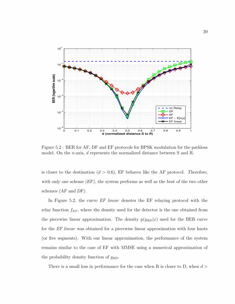
39

0 0.1 0.2 0.3 0.4 0.5 0.6 0.7 0.8 0.9 110

−5

10−4

10−3

10−2

10−1

100

d (normalized distance S to R)

BE

R (l

ogar

ithm

sca

le)

no Relay

DF

AF

EF − E[x|y]

EF linear

Figure 5.2 : BER for AF, DF and EF protocols for BPSK modulation for the pathlossmodel. On the x-axis, d represents the normalized distance between S and R.

is closer to the destination (d > 0.6), EF behaves like the AF protocol. Therefore,

with only one scheme (EF), the system performs as well as the best of the two other

schemes (AF and DF).

In Figure 5.2, the curve EF linear denotes the EF relaying protocol with the

relay function fEF , where the density used for the detector is the one obtained from

the piecewise linear approximation. The density p(yRD|x) used for the BER curve

for the EF linear was obtained for a piecewise linear approximation with four knots

(or five segments). With our linear approximation, the performance of the system

remains similar to the case of EF with MMSE using a numerical approximation of

the probability density function of yRD.

There is a small loss in performance for the case when R is closer to D, when d >

40

0.1 0.2 0.3 0.4 0.5 0.6 0.7 0.8 0.9 110

−4

10−3

10−2

10−1

100

d (normalized distance S to R)

SE

R (

log

arit

hm

sca

le)

no Relay

DF

AF

EF − MMSE

EF − linear

Figure 5.3 : SER for AF, DF and EF protocols for 16QAM modulation for the pathlossmodel. On the x-axis, d represents the normalized distance between S and R.

0.7. This is due to using an approximation of the density p(yRD|x). The performance

of the system is strictly related to the accuracy of the piecewise linear approximation

used to derive the density of yRD.

In Figure 5.3, the SER is plotted for all analyzed relaying protocols. The line

denoted as no Relay, represents the SER obtained for the direct link, when no coop-

eration is employed. For fairness of the comparison, we assumed the power used by

the source is equal to the total power used in the cooperative case, that is, equal to

source power(PS) plus relay power(PR). In the case of increasing the source modula-

tion order to 16 QAM, the same trends are observed for the EF - MMSE and EF -

linear as when BPSK modulation is used. The piecewise linear approximation used

for the 16 QAM SER results employed a 20-knot discretization.

41

The properties of the MMSE estimate are preserved for higher order modulation as

expected from the way the MMSE behaves, see Figure 4.3. Also, the linear piecewise

approximation of the MMSE estimate preserves the properties of the MMSE, its

overall performance follows the best of the AF and DF.

42

Chapter 6

Conclusions

In this work we have investigated the performance of the EF protocol with MMSE

estimate as the relay function. In a pathloss model and for both BPSK and 16 QAM

modulation, EF with this type of soft information performs as well as the best of AF

and DF. When R is close to S, EF performs like DF, while when R is closer to D, it

performs like AF. However, this performance comes at a price; the conditional prob-

ability density function of the received signal at the source from the relay, p(yRD|x)

does not have an analytical form. Therefore, the detector at the destination can be

implemented only by using a density obtained through numerical computation. We

have shown that the need for this density can be avoided by employing a piecewise

linear approximation of the MMSE estimate as the relay function. With this linear

approximation, the density of the received symbol at the destination has an analytical

form and thus, so does the detector. In conclusion, we do not only offer another type

of soft information which can be used in the EF relay protocol, we also provide an

analytical form of the optimal detector at the destination. Simulation results with

SER as the performance metric confirmed the theoretical results.

43

Appendix A

In this Appendix, we focus on presenting in detail the steps for deriving the final

form of the pdf p(yRD|x). This density has slightly different forms depending on the

region of integration.

Using the conditional probability density function of yRD given ySR from equation

(4.29) in (4.28) we obtain the density,

p(yRD|x) =

∫ y1

−∞N (m1, 1)N (hSRx, 1)dySR (A.1)

+n∑i=2

∫ yi

yi−1

N (mi, 1)N (hSRx, 1)dySR

+

∫ +∞

yn

N (mn+1, 1)N (hSRx, 1)dySR

where mi is the mean given in (4.30). This density is split into three different cases,

depending on the region of integration. Two cases are unique, the ones corresponding

to the extremities, ySR ∈ (− inf, y1) and ySR ∈ (yn,+ inf), which are particular cases

of the most general one given by ySR ∈ (yi−1, yi). We focus on the case when ySR is

between two knots, that is ySR ∈ (yi−1, yi). This case is the most general one, and

all other regions represent particular cases of this one. We focus on the general case,

which is equivalent to the following part of the density given in (A.1), where we used

the mean mi given in (4.30) :

p(yRD|x) =

∫ yi

yi−1

N (hRDk(aiySR + bi), 1)N (hSRx, 1)dySR, for ySR ∈ (yi−1, yi).(A.2)

44

Next, we expand the Gaussian densities:

p(yRD |x) = (A.3)∫ yi

yi−1

1√2π

exp

{−(yRD − hRDk(aiySR + bi))

2

2

}1√2π

exp

{−(ySR − hSRx)2

2

}dySR

=

∫ yi

yi−1

(1√2π

)2

exp

{−1

2

[y2RD − 2yRDhRDk(aiySR + bi) + h2RDk

2(aiySR + bi)2

+(y2SR − 2hSRxySR + h2SRx

2)]}

dySR. (A.4)

The next step is to group the terms with respect to the powers of ySR and use the

following notation :

Ai =1

h2RDk2a2i + 1

(A.5)

Bi(yRD, x) = hRDkai(yRD − hRDkbi) + hSRx (A.6)

Ci(yRD, x) = (yRD − hRDkbi)2 + h2SRx2. (A.7)

With this notation, the probability density function for this region becomes:

p(yRD|x) = (A.8)∫ yi

yi−1

(1√2π

)2

exp

{−1

2Ci(yRD, x)

}exp

{−1

2

(1

Aiy2SR − 2Bi(yRD, x)ySR

)}dySR.

Since the exponent of the first term does not depend on ySR, it can be taken outside

the integral and we complete the square with respect to variable ySR:

p(yRD|x) = (A.9)(1√2π

)2

exp

{−Ci(yRD, x)

2

}∫ yi

yi−1

exp

{−(ySR −Bi(yRD, x)Ai)

2

2Ai+B2i (yRD, x)Ai

2

}dySR.

The second term of the exponential does not depend on ySR, so it will be taken

outside the integral. We are left with a finite integral of a Gaussian density, thus we

45

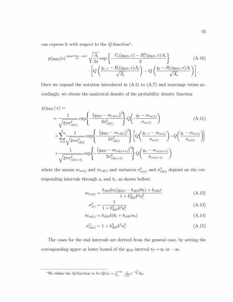
can express it with respect to the Q-function∗:

p(yRD|x)ySR∈(yi−1,yi)

=

√Ai2π

exp

{−Ci(yRD, x)−B2

i (yRD, x)Ai2

}(A.10)

·[Q

(yi−1 −Bi(yRD, x)Ai√

Ai

)−Q

(yi −Bi(yRD, x)Ai√

Ai

)].

Once we expand the notation introduced in (A.5) to (A.7) and rearrange terms ac-

cordingly, we obtain the analytical density of the probability density function

p(yRD |x) =

=1√

2πσ2rd(1)

exp

{−(yRD −mrd(1)

)22σ2

rd(1)

}Q

(−y1 −msr(1)

σsr(1)

)(A.11)

+n∑i=2

1√2πσ2

rd(i)

exp

{−(yRD −mrd(i)

)22σ2

rd(i)

}[Q

(yi−1 −msr(i)

σsr(i)

)−Q(yi −msr(i)

σsr(i)

)]

+1√

2πσ2rd(n+1)

exp

{−(yRD −mrd(n+1)

)22σ2

rd(n+1)

}Q

(yn −msr(n+1)

σsr(n+1)

)

where the means msr(i) and mrd(i) and variances σ2sr(i) and σ2

rd(i) depend on the cor-

responding intervals through ai and bi, as shown bellow:

msr(i) =hRDkai(yRD − hRDkbi) + hSRx

1 + h2RDk2a2i

(A.12)

σ2sri =

1

1 + h2RDk2a2i

(A.13)

mrd(i) = hRDk(bi + hSRxai) (A.14)

σ2rd(i) = 1 + h2RDk

2a2i . (A.15)

The cases for the end intervals are derived from the general case, by setting the

corresponding upper or lower bound of the ySR interval to +∞ or −∞.

∗We define the Q-function to be Q(α) =∫ +∞α

1√2πe−

ω2

2 dω.

46

Bibliography

[1] E. C. van der Meulen, “Three-terminal communication channels,” Adv. Appl.

Probab., vol. 3, pp. 120–154, 1971.

[2] T. Cover and A. Gamal, “Capacity theorems for the relay channel,” IEEE Trans-

actions on Information Theory, vol. 25, no. 5, pp. 572–584, Sept. 1979.

[3] G. Kramer, M. Gastpar, and P. Gupta, “Cooperative strategies and capacity

theorems for relay networks,” IEEE Transactions on Information Theory, vol. 51,

no. 9, pp. 3037–3063, Sept. 2005.

[4] A. Host-Madsen, “Capacity bounds for cooperative diversity,” IEEE Transactions

on Information Theory, vol. 52, no. 4, pp. 1522 –1544, April 2006.

[5] L. Lai, K. Liu, and H. El Gamal, “The three-node wireless network: achievable

rates and cooperation strategies,” IEEE Transactions on Information Theory,

vol. 52, no. 3, pp. 805 –828, March 2006.

[6] A. Sendonaris, E. Erkip, and B. Aazhang, “User cooperation diversity - Part I:

System description,” IEEE Transactions on Communications, vol. 51, no. 11, pp.

1927–1938, 2003.

[7] ——, “User cooperation diversity - Part II: Implementation aspects and perfor-

mance analysis,” IEEE Transactions on Communications, vol. 51, no. 11, pp.

1939–1948, 2003.

47

[8] J. Laneman, D. Tse, and G. Wornell, “Cooperative diversity in wireless networks:

Efficient protocols and outage behavior,” IEEE Transactions on Information The-

ory, vol. 50, no. 12, pp. 3063–3080, Dec. 2004.

[9] J. N. Laneman and G. Wornell, “Energy-efficient antenna sharing and relaying

for wireless networks,” in Wireless Communications and Networking Conference,

2000. WCNC. 2000 IEEE, vol. 1, Chicago, IL , USA, 2000, pp. 7–12.

[10] M. Yuksel and E. Erkip, “Diversity in relaying protocols with amplify and for-

ward,” in GLOBECOM ’03. IEEE Global Telecommunications Conference 2003,

vol. 4, Dec. 2003, pp. 2025 – 2029.

[11] ——, “Multiple-antenna cooperative wireless systems: A diversity-multiplexing

tradeoff perspective,” IEEE Transactions on Information Theory, vol. 53, no. 10,

pp. 3371 –3393, Oct. 2007.

[12] J. N. Laneman, “Cooperative diversity in wireless networks: Algorithms and

architectures,” Ph.D. dissertation, Massachusetts Institute of Technology, Cam-

bridge, MA, August 2003.

[13] M. Souryal and B. Vojcic, “Performance of amplify-and-forward and decode-and-

forward relaying in rayleigh fading with turbo codes,” in Proceedings of IEEE

International Conference on Acoustics, Speech and Signal Processing, ICASSP

2006, vol. 4, may. 2006, pp. IV –IV.

[14] P. Herhold, E. Zimmermann, and G. Fettweis, “On the performance of cooper-

ative amplify-and-forward relay networks,” in in Proceedings of the International

ITG Conference on Source and Channel Coding (SCC’04), Erlangen, Germany,

Jan 2004, pp. 451–458.

48

[15] D. Chen, K. Azarian, and J. Laneman, “A case for amplify and forward re-

laying in the block-fading multiple-access channel,” Information Theory, IEEE

Transactions on, vol. 54, no. 8, pp. 3728 –3733, aug. 2008.

[16] A. Chakrabarti, A. Sabharwal, and B. Aazhang, “Quantizer design and imple-

mentation of estimate-and-forward relaying,” in preparation for IEEE Transac-

tions on Communications.

[17] I. Abou-Faycal and M. Medard, “Optimal uncoded regeneration for binary an-

tipodal signaling,” in IEEE International Conference on Communications, vol. 2,

Jun. 2004, pp. 742 – 746.

[18] K. S. Gomadam and S. A. Jafar, “Optimal relay functionality for SNR maximiza-

tion in memoryless relay networks,” IEEE Journal on Selected Areas in Commu-

nications, vol. 25, no. 2, pp. 390 –401, Feb. 2007.

[19] K. Gomadam and S. Jafar, “On the capacity of memoryless relay networks,”

vol. 4, Jun. 2006, pp. 1580 –1585.

[20] T. Cui, T. Ho, and J. Kliewer, “Some results on relay strategies for memoryless

two-way relay channels,” in 2008 Information Theory and Applications Workshop,

Jan. 2008, pp. 158 –164.

[21] P. Weitkemper, D. Wubben, and K.-D. Kammeyer, “Minimum mse relaying in

coded networks,” in WSA 2008. International ITG Workshop on Smart Antennas,

Feb. 2008, pp. 96 –103.

[22] ——, “Minimum mse relaying for arbitrary signal constellations in coded relay

networks,” in VTC Spring 2009. IEEE 69th Vehicular Technology Conference,

April 2009, pp. 1 –5.

49

[23] M. Khormuji and E. Larsson, “Receiver design for wireless relay channels with

regenerative relays,” in ICC ’07. IEEE International Conference on Communica-

tions 2007, June 2007, pp. 4034 –4039.

[24] M. Khormuji and M. Skoglund, “On instantaneous relaying,” IEEE Transactions

on Information Theory, vol. 56, no. 7, pp. 3378 –3394, Jul. 2010.

[25] T. Wang, A. Cano, G. Giannakis, and J. Laneman, “High-performance coop-

erative demodulation with decode-and-forward relays,” IEEE Transactions on

Communications, vol. 55, no. 7, pp. 1427 –1438, July 2007.

[26] F. Hu and J. Lilleberg, “Novel soft symbol estimate and forward scheme in

cooperative relaying networks,” in 2009 IEEE 20th International Symposium on

Personal, Indoor and Mobile Radio Communications, Sept 2009, pp. 2691 –2694.

[27] S. Tian, Y. Li, and B. Vucetic, “Piecewise-and-forward relaying in wireless relay

networks,” IEEE Signal Processing Letters, vol. 18, no. 5, pp. 323 –326, May 2011.

[28] A. Ribeiro, X. Cai, and G. Giannakis, “Symbol error probabilities for general

cooperative links,” IEEE Transactions on Wireless Communications, vol. 4, no. 3,

pp. 1264 – 1273, May 2005.

[29] R. U. Nabar, H. Bolcskei, and F. W. Kneubuhler, “Fading relay channels: per-

formance limits and space-time signal design.” IEEE Journal on Selected Areas

in Communications, vol. 22, no. 6, pp. 1099–1109, 2004.

[30] A. Papoulis and S. Pillai, Probability, Random Variables and Stochastic Pro-

cesses, 4th ed. McGraw Hill Higher Education, .

50

[31] C. Berger, P. Willett, S. Zhou, and P. Swaszek, “Deflection-optimal data for-

warding over a Gaussian multiaccess channel,” IEEE Communications Letters,

vol. 11, no. 1, pp. 1 –3, Jan. 2007.

[32] G. W. Stewart, Afternotes goes to Graduate School - : Lectures on Advanced

Numerical Analysis. SIAM, 1998.

[33] D. Brennan, “Linear diversity combining techniques,” Proceedings of the IRE,

vol. 47, no. 6, pp. 1075–1102, June 1959.

[34] M. D. Godfrey, “The TANH transformation,” Information System Laboratory

EE Department at Stanford University.