1

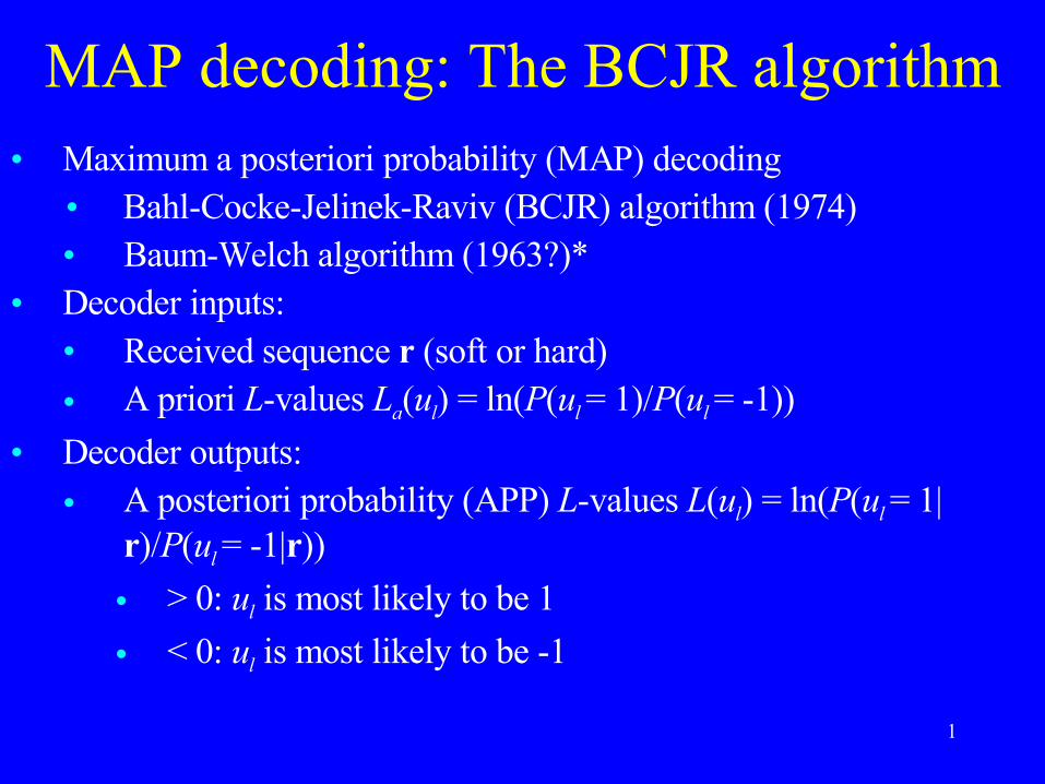
MAP decoding: The BCJR algorithm• Maximum a posteriori probability (MAP) decoding

• Bahl-Cocke-Jelinek-Raviv (BCJR) algorithm (1974)• Baum-Welch algorithm (1963?)*

• Decoder inputs:• Received sequence r (soft or hard)• A priori L-values La(ul) = ln(P(ul = 1)/P(ul = -1))

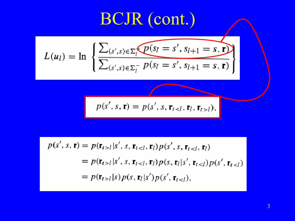
• Decoder outputs:• A posteriori probability (APP) L-values L(ul) = ln(P(ul = 1|

r)/P(ul = -1|r))• > 0: ul is most likely to be 1• < 0: ul is most likely to be -1

2

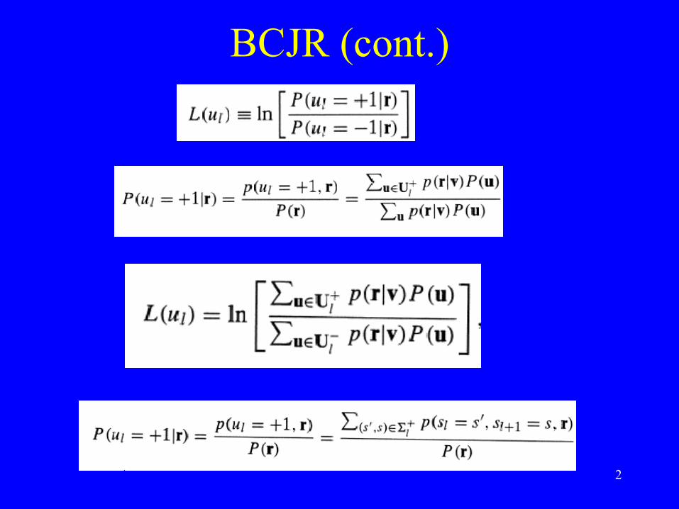
BCJR (cont.)

3

BCJR (cont.)

4

BCJR (cont.)

5

BCJR (cont.)

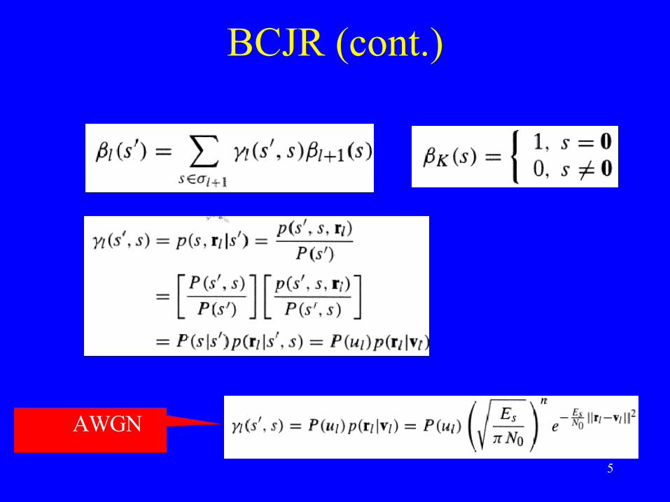
AWGN

6

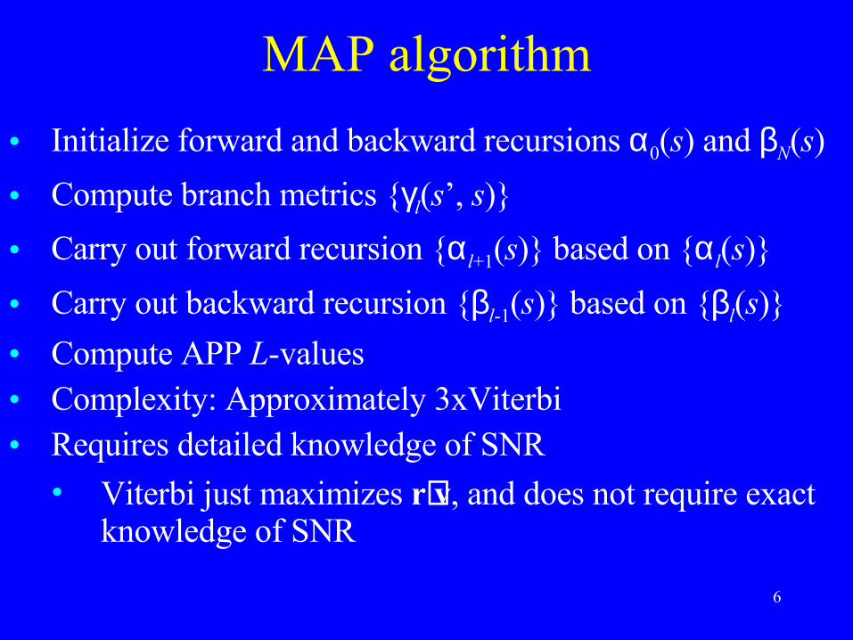
MAP algorithm• Initialize forward and backward recursions α0(s) and βN(s)• Compute branch metrics {γl(s’, s)}• Carry out forward recursion {αl+1(s)} based on {αl(s)}• Carry out backward recursion {βl-1(s)} based on {βl(s)}• Compute APP L-values• Complexity: Approximately 3xViterbi• Requires detailed knowledge of SNR

• Viterbi just maximizes r⋅v, and does not require exact knowledge of SNR

7

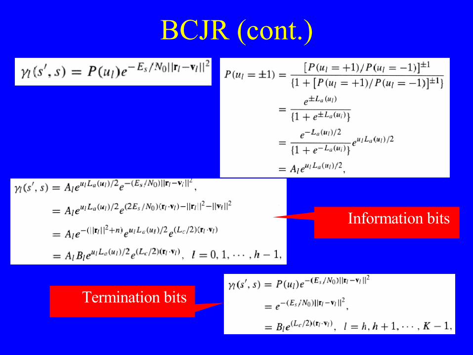
BCJR (cont.)

Information bits

Termination bits

8

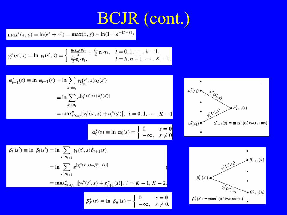
BCJR (cont.)

9

BCJR (cont.)

10

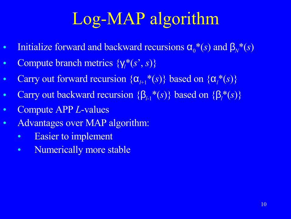
Log-MAP algorithm• Initialize forward and backward recursions α0*(s) and βN*(s)• Compute branch metrics {γl*(s’, s)}• Carry out forward recursion {αl+1*(s)} based on {αl*(s)}• Carry out backward recursion {βl-1*(s)} based on {βl*(s)}• Compute APP L-values• Advantages over MAP algorithm:

• Easier to implement• Numerically more stable

11

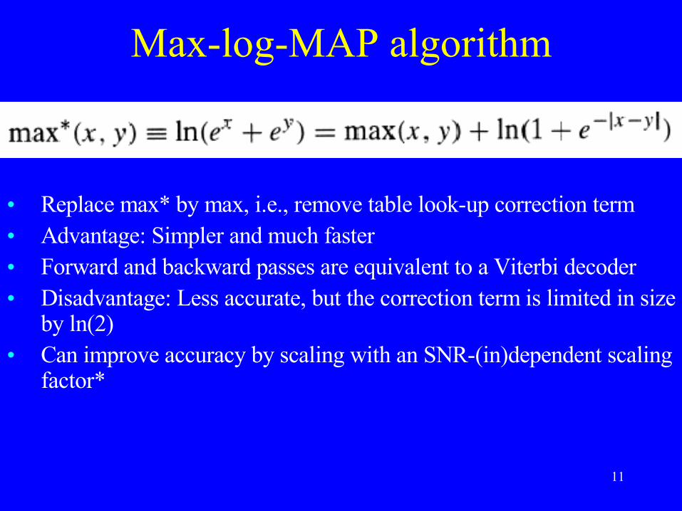
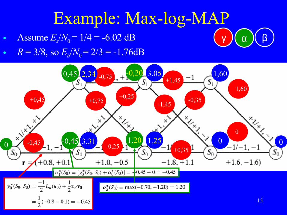
Max-log-MAP algorithm

• Replace max* by max, i.e., remove table look-up correction term• Advantage: Simpler and much faster• Forward and backward passes are equivalent to a Viterbi decoder• Disadvantage: Less accurate, but the correction term is limited in size

by ln(2)• Can improve accuracy by scaling with an SNR-(in)dependent scaling

factor*

12

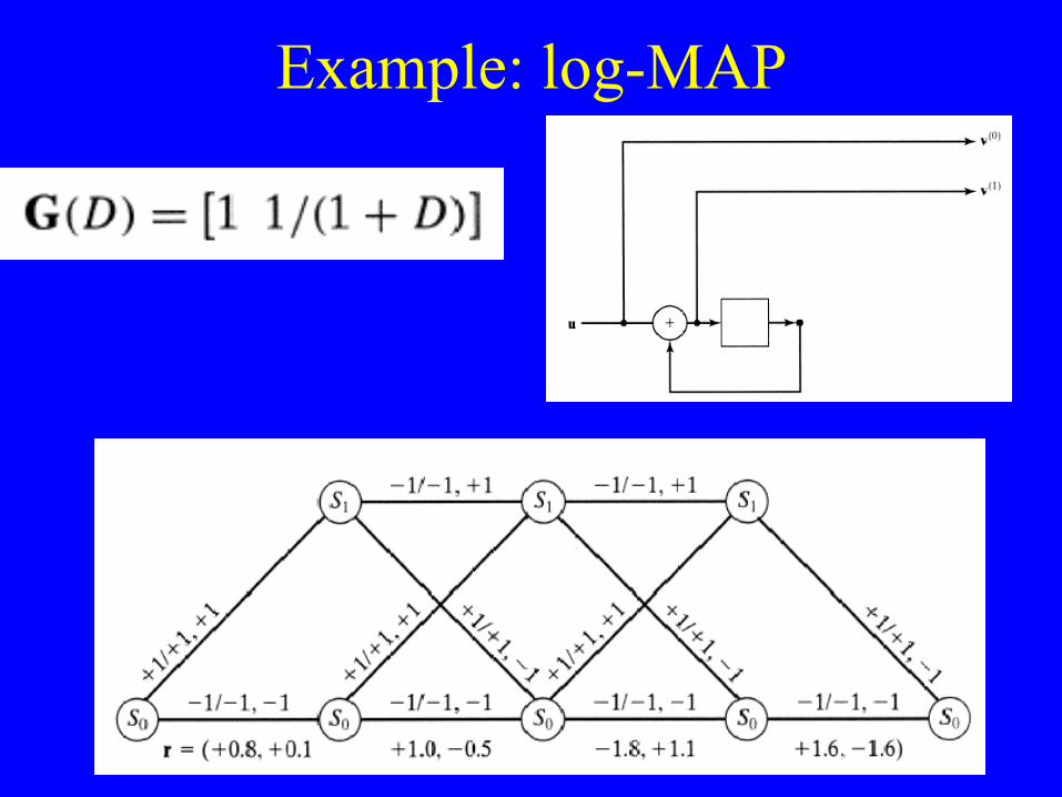
Example: log-MAP

13

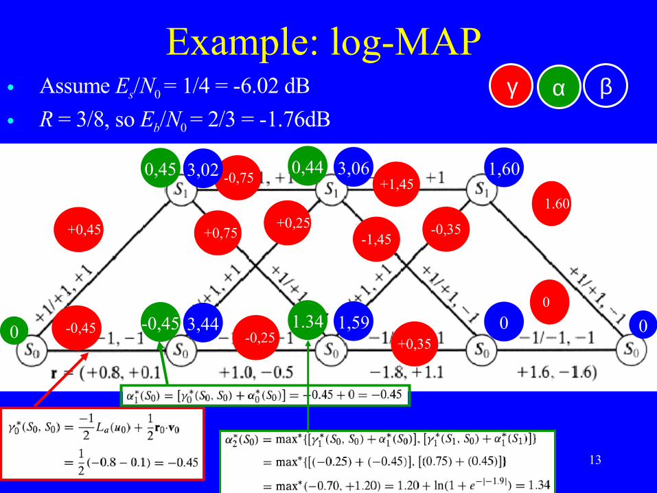
Example: log-MAP • Assume Es/N0 = 1/4 = -6.02 dB• R = 3/8, so Eb/N0 = 2/3 = -1.76dB

-0,45

+0,45

-0,25

+0,25

-0,75

+0,75

+0,35

-0,35

+1,45

-1,45

0

1.60

0 0

1,60

0 1,59

3,06

3,44

3,02

β α γ

-0,45

0,45

1.34

0,44

14

Example: log-MAP • Assume Es/N0 = 1/4 = -6.02 dB• R = 3/8, so Eb/N0 = 2/3 = -1.76dB

-0,45

+0,45

-0,25

+0,25

-0,75

+0,75

+0,35

-0,35

+1,45

-1,45

0

1.60

0 0

1,60

0 1,59

3,06

3,44

3,02

β α γ

-0,45

0,45

1.34

0,44

+0.48 +0.62 -1,02

15

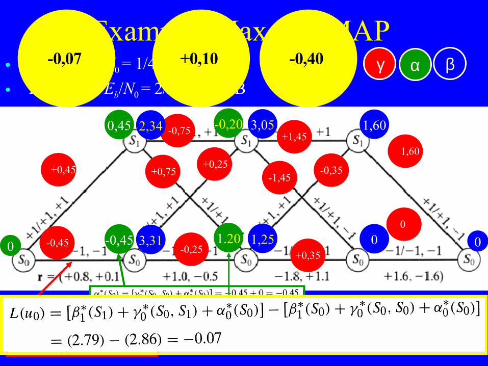
Example: Max-log-MAP • Assume Es/N0 = 1/4 = -6.02 dB• R = 3/8, so Eb/N0 = 2/3 = -1.76dB

-0,45

+0,45

-0,25

+0,25

-0,75

+0,75

+0,35

-0,35

+1,45

-1,45

0

1,60

0 0

1,60

0 1,25

3,05

3,31

2,34

β α γ

-0,45

0,45

1.20

-0,20

16

Example: Max-log-MAP • Assume Es/N0 = 1/4 = -6.02 dB• R = 3/8, so Eb/N0 = 2/3 = -1.76dB

-0,45

+0,45

-0,25

+0,25

-0,75

+0,75

+0,35

-0,35

+1,45

-1,45

0

1,60

0 0

1,60

0 1,25

3,05

3,31

2,34

β α γ

-0,45

0,45

1.20

-0,20

-0,07 +0,10 -0,40

17

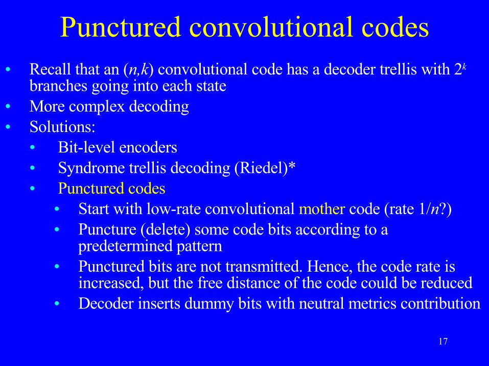
Punctured convolutional codes• Recall that an (n,k) convolutional code has a decoder trellis with 2k

branches going into each state• More complex decoding• Solutions:

• Bit-level encoders• Syndrome trellis decoding (Riedel)*• Punctured codes

• Start with low-rate convolutional mother code (rate 1/n?)• Puncture (delete) some code bits according to a

predetermined pattern• Punctured bits are not transmitted. Hence, the code rate is

increased, but the free distance of the code could be reduced• Decoder inserts dummy bits with neutral metrics contribution

18

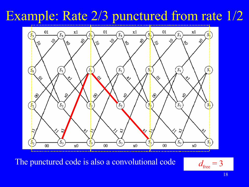
Example: Rate 2/3 punctured from rate 1/2

The punctured code is also a convolutional code dfree = 3

19

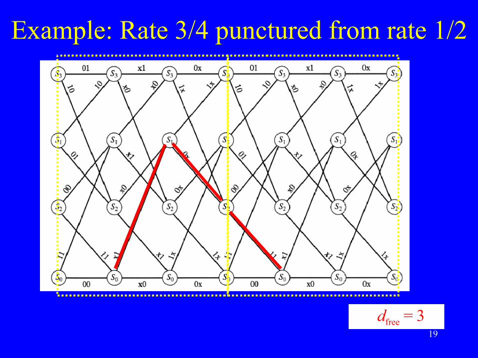
Example: Rate 3/4 punctured from rate 1/2

dfree = 3

20

More on punctured convolutional codes• Rate-compatible punctured convolutional (RCPC) codes:

• Used for applications that need to support several code rates, e.g., adaptive coding or hybrid ARQ

• Sequence of codes is obtained by repeated puncturing • Advantage: One decoder can decode all codes in the family• Disadvantage: Resulting codes may be sub-optimum

• Puncturing patterns:• Usually periodic puncturing patterns• Found by computer search• Care must be exercised to avoid catastrophic encoders

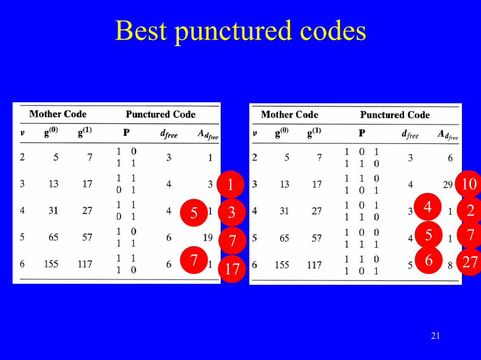
21

Best punctured codes

1

5 3

7 7 17

10 4 2

6 27 7 5

22

Tailbiting convolutional codes• Purpose: Avoid the terminating tail (rate loss) and maintain a

uniform level of protection• Note: Cannot avoid distance loss completely unless the length is

not too short. When the length gets larger, the minimum distance approaches the free distance of the convolutional code

• Codewords can start in any state• This gives 2ν as many codewords• However, each codeword must end in the same state that it

started from. This gives 2-ν as many codewords• Thus, the code rate is equal to the encoder rate

• Tailbiting codes are increasingly popular for moderate length purposes

• Some of the best known linear block codes are tailbiting codes• Tables of optimum tailbiting codes are given in the book• DVB: Turbo codes with tailbiting component codes

23

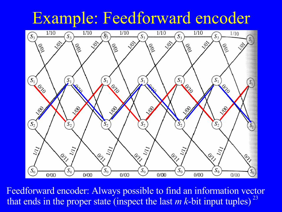
Example: Feedforward encoder

Feedforward encoder: Always possible to find an information vector that ends in the proper state (inspect the last m k-bit input tuples)

24

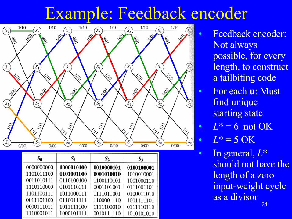
Example: Feedback encoder• Feedback encoder:

Not always possible, for every length, to construct a tailbiting code

• For each u: Must find unique starting state

• L* = 6 not OK• L* = 5 OK• In general, L*

should not have the length of a zero input-weight cycle as a divisor

25

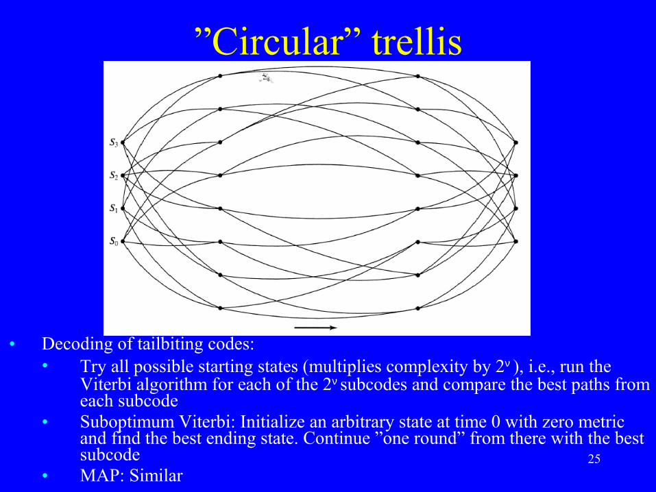
”Circular” trellis

• Decoding of tailbiting codes:• Try all possible starting states (multiplies complexity by 2ν ), i.e., run the

Viterbi algorithm for each of the 2ν subcodes and compare the best paths from each subcode

• Suboptimum Viterbi: Initialize an arbitrary state at time 0 with zero metric and find the best ending state. Continue ”one round” from there with the best subcode

• MAP: Similar