Many-Body effects in Semiconductor Nanostructureslindroth/CarlWesslen_lic.pdf · Many-Body e ects in Semiconductor Nanostructures ... the 1D quantum wire (green) and the 0D quantum

Stockholm University

Licentiat Thesis

Many-Body effects in SemiconductorNanostructures

Author:

Carl Wesslen

Supervisor:

Prof. Eva Lindroth

Akademisk avhandling for avlaggande av

licentiatexamen i fysik vid Stockholms Universitet

April 2014

http://www.su.se

“For nar som faran ar som storst,

sa raddas man av kaffetorst.”

Ronny Astrom

STOCKHOLM UNIVERSITY

Abstract

Faculty of Science

Department of Physics

Teknologie Licentiat

Many-Body effects in Semiconductor Nanostructures

by Carl Wesslen

Low dimensional semiconductor structures are modeled using techniques from the field of

many-body atomic physics. B-splines are used to create a one-particle basis, used to solve

the more complex many-body problems. Details on methods such as the Configuration

Interaction (CI), Many-Body Perturbation Theory (MBPT) and Coupled Cluster (CC)

are discussed. Results from the CC singles and doubles method are compared to other

high-precision methods for the circular harmonic oscillator quantum dot. The results

show a good agreement for the energy of many-body states of up to 12 electrons.

Properties of elliptical quantum dots, circular quantum dots, quantum rings and concen-

tric quantum rings are all reviewed. The effects of tilted external magnetic fields applied

to the elliptical dot are discussed, and the energy splitting between the lowest singlet

and triplet states is explored for varying geometrical properties. Results are compared

to experimental energy splittings for the same system containing 2 electrons.

http://www.su.se

http://www.science.su.se/english/

http://www.fysik.su.se

Contents

Abstract ii

Contents iii

List of Papers iv

1 Introduction 1

1.1 Low Dimensional Semiconductor Structures . . . . . . . . . . . . . . . . . 1

2 Computational Methods 4

2.1 One-Particle Treatment . . . . . . . . . . . . . . . . . . . . . . . . . . . . 4

2.1.1 Polar coordinates . . . . . . . . . . . . . . . . . . . . . . . . . . . . 5

2.1.2 Cartesian coordinates . . . . . . . . . . . . . . . . . . . . . . . . . 7

2.1.3 B-spline Basis . . . . . . . . . . . . . . . . . . . . . . . . . . . . . . 8

2.1.4 Magnetic Field . . . . . . . . . . . . . . . . . . . . . . . . . . . . . 10

2.2 Many-Body Treatment . . . . . . . . . . . . . . . . . . . . . . . . . . . . . 12

2.2.1 Configuration Interaction . . . . . . . . . . . . . . . . . . . . . . . 13

2.2.2 Perturbation Theory . . . . . . . . . . . . . . . . . . . . . . . . . . 15

2.2.3 Coupled Cluster . . . . . . . . . . . . . . . . . . . . . . . . . . . . 22

3 Effective Potentials 25

3.1 Quantum Dot . . . . . . . . . . . . . . . . . . . . . . . . . . . . . . . . . . 25

3.1.1 Harmonic Oscillator . . . . . . . . . . . . . . . . . . . . . . . . . . 26

3.1.2 Elliptic Harmonic Oscillator . . . . . . . . . . . . . . . . . . . . . . 28

3.1.3 Hard Wall . . . . . . . . . . . . . . . . . . . . . . . . . . . . . . . . 31

3.2 Quantum Ring . . . . . . . . . . . . . . . . . . . . . . . . . . . . . . . . . 32

3.2.1 Concentric Rings . . . . . . . . . . . . . . . . . . . . . . . . . . . . 33

4 Outlook 35

4.1 Outlook . . . . . . . . . . . . . . . . . . . . . . . . . . . . . . . . . . . . . 35

Acknowledgements 36

Bibliography 37

Paper I 40

Paper II 52

iii

List of Papers

Paper I Performance of the coupled-cluster singles and doubles method

applied to two-dimensional quantum dots

E. Waltersson, C. J. Wesslen, and E. Lindroth

Physical Review B, 87, 035112 (2013). DOI: 10.1103/PhysRevB.87.035112

Paper II Two-electron quantum dot in tilted magnetic fields:

Sensitivity to the confinement model

T. Frostad, J. P. Hansen, C. J. Wesslen, E. Lindroth and E. Rasanen

The European Physical Journal B, 86(10), 1-6 (2013).

DOI: 10.1140/epjb/e2013-40677-x

iv

Chapter 1

Introduction

1.1 Low Dimensional Semiconductor Structures

Low dimensional semiconductor structures are key building blocks in modern electronic

technology, being the basis of several applications such as solar cells, light-emitting

diodes and transistors. Quantum mechanical effects are of special importance in semi-

conductor structures and a proper understanding of these become important when cre-

ating more complex devices.

The important properties of semiconductor materials lie in the so called band structure.

By adjusting the availability of electrons in the conduction band and holes in the valance

band, control of the materials conductivity may be achieved. This is often done by doping

the semiconductor, placing impurities into the bulk and thereby injecting conductive

electrons or holes into the band structure.

The conducting particles in a semiconductor material, such as electrons in the conduction

band or holes in the valence band, can usually be modeled as a free electron gas. If one

constrains the motion of the particles, only allowing them to move in two of the material’s

three dimensions, a partial quantization of energy is achieved. The resulting potential

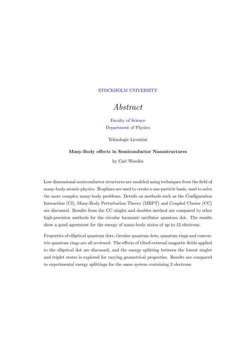
is called a quantum-well, the density of state of which can be seen in Fig. 1.1. By

constraining the particle motion to one and then zero dimensions further quantization

occurs until one has fully discretized energy levels in the zero-dimensional quantum dot.

Details regarding this can be found in most textbooks on semiconductor physics, such as

[1]. The term Quantum Dot (QD) was introduced in [2], and has become an established

term when describing highly constrained, artificial, atom like systems. QD:s are not

only formed by low dimensional semi conductor structures, however these are the ones

handled in this thesis.

1

Chapter 1. Introduction 2

Energy [arb. unit]

Den

sity

of st

ate

s [a

rb. unit]

Figure 1.1: Density of states for the 3D bulk semiconductor material (blue), the 2Dquantum well (red), the 1D quantum wire (green) and the 0D quantum dot (black).One sees that as the motion of the conducting particles is limited, the energy levels are

further and further quantized.

Discretized energy levels are normally something you find in atoms, but in the quantum

dot they come with the advantage of being adjustable. The effective potential con-

structed due to the 0D confinement of the dot will largely determine the energy level

structure in the dot, but also material properties such as the effective electron mass and

the material’s dielectric constant come into effect. A more detailed discussion regarding

the shape of the effective potential, and the effects of these on the conducting electrons,

can be found in Chapter ??.

Another property that the quantum dot shares with the atom is the existence of a shell

structure. Much as the noble gases of the periodic table, quantum dots with certain

numbers of confined electrons also display spikes in addition energy, i. e. the energy

required to ad another electron to the system. This was experimentally demonstrated

by Tarucha in 1996 [3], and has been subject to many theoretical studies as reviewed

in [4]. When calculating the addition energy spectra for the electrons in the quantum

dot, precise calculations of the Coulomb interaction is required. Methods of handling

these are discussed in Chapter 3 of the thesis and the results from one such method, the

Coupled Cluster Singles and Doubles method, are presented in paper I.

Chapter 1. Introduction 3

The effects of an applied magnetic field to a QD are of great importance when manufac-

turing spintronic devices, and are also discussed in the thesis. In paper II, experimental

results by Meunier on an elliptical QD with a tilted magnetic field, [5], are compared to

theoretical results.

These atom-like properties give the QD:s the name artificial atoms, and many theoret-

ical methods used in atomic physics are also very suitable when handling them. But

semiconductors can also be used to form more exotic potential structures, displaying

qualities usually not found in nature. An example of such a system is the Quantum

Ring (QR). The QR is a toroid (donut-shaped) potential, where the electrons are con-

fined in a ring of arbitrary size. The two extreme limits of the ring are; a dot in the case

of a ring with zero radius, and a quantum wire for a ring of infinite radius. By adjusting

the QR:s features, it can have different interesting properties. Experimentally rings of

different shapes and sizes have been manufactured in a number of ways, [6, 7], one of

the more exotic being the concentric rings manufactured by Mano in 2002, [8]. Both

normal quantum rings and concentric quantum rings are discussed more in Chapter ??.

The science of low dimensional semiconductor structures is still quite young and the

full potential has not yet fully been explored. Except applications such as those already

mentioned, a novel area of use is in quantum computing. Quantum computing is a hot

topic that can be read about in most popular science literature and can be reviewed in

[9]. A key component behind a quantum computer is the so called quantum bit, or qbit.

Quantum dots are one of several qbit candidates, exhibiting desired qualities such as

coherence and high controllability. Success in implementing them will however require a

great deal of experimental technique and theoretical understanding of their properties.

Chapter 2

Computational Methods

2.1 One-Particle Treatment

Here the one-electron quantum dot is introduced and the corresponding single-particle

Hamiltonian is defined to calculate the systems eigenstates and energies. The one-

electron eigenstates will form a basis later to be used when treating the many electron

dot and will include all effects except the electron-electron interaction, which will be

added in in section 2.2.

The one particle Hamiltonian in a magnetic field reads:

hop =1

2m∗(−i~∇+ eA)2 + V (x), (2.1)

where A is the field vector potential and V (x) is the effective potential of the dot. Both

A and V will be discussed in further detail later on. The focus for now will be on the

case of no magnetic field and V being a two dimensional harmonic oscillator potential.

The Hamiltonian now reads:

hop(r) =p2

2m∗+

1

2m∗ω2r2, (2.2)

4

Chapter 2. Computational Methods 5

in polar coordinates and:

hop(x) =p2

2m∗+

1

2m∗ω2(x2 + y2), (2.3)

in Cartesian coordinates.

Inserting the Hamiltonian into the Schrodinger equation,

hopΨ = εΨ, (2.4)

one hopes to find the wave functions Ψ and their corresponding energies ε.

2.1.1 Polar coordinates

As the 2D harmonic oscillator potential has a cylindrical symmetry, it is natural to solve

the problem using polar coordinates. Since the Hamiltonian is separable in a radial part

and an angular part one expects to find solutions of the form:

Ψnmlms(r, φ) = unmlms(r)eimlφ|ms〉, (2.5)

divided into a radial part unmlms , an angular part, eimlφ and a spin part |ms〉.

The non trivial part to solve now is the radial eigenvalue problem:

[~2

2m∗(−←−∂r−→∂r +

m2l

2r2) +

1

2m∗ω2r2

]unml

(r) = εnmlunml

(r), (2.6)

Where←−∂r and

−→∂r represent differential operators working to the left or right respectively.

Solving this, one finds the wave functions to eq. 2.4:

Ψnml(r, φ) =

1

l

√2n!

n+ |ml|!

(rl

)|ml|L|ml|n ((r/l)2)e−(r2/2l2) e

imlφ

√2π

(2.7)


n,ml=0,1n,ml=0,1

n,ml=1,1n,ml=1,0

Figure 2.1: Plots of the real part of four of the wave functions acquired using eq. 2.7,labeled using the n and ml quantum numbers.

and the corresponding eigenvalues:

εnml= ~ω(2n+ |ml|+ 1). (2.8)

Where L|ml|n are the associated Laguerre polynomials, and l is the typical harmonic

oscillator length: l =√

~mω .

Details on how eq. 2.6 is solved can be found in quantum mechanical textbooks such as

[10]. The real part of some of these wave functions can be seen in figure 2.1.

The polar solution is powerful since it has a trivial solution in the angular regime,

reducing our problem from two dimensions into one radial dimension. This solution

is also useful when introducing a magnetic field, since these states are also eigenstates

to the Lz operator. However any change to the potential that breaks the cylindrical

symmetry, such as the elliptical dot or the tilted magnetic field introduced later on,


disables us from using the cylindrical symmetry property required for this separation

into an angular and a radial part.

2.1.2 Cartesian coordinates

By solving the the Schrodinger equation in Cartesian coordinates the problem separates

into two one dimensional harmonic oscillator potentials:

1

2m∗∂2

∂x2ψnx(x) +

1

2m∗ω2x2ψnx(x) = εnxψnx(x), (2.9)

for the x and y coordinate separately. The solution, once again in atomic units, has the

eigenstates:

ψnx(x) =1√

2nxnx!

(mωπ~

)1/4Hnx(mωx/~)e−mωx

2/2~, (2.10)

where Hnx(x) are Hermite polynomials. And the eigenvalues are:

εnx = ~ω(nx +1

2) (2.11)

The solution to the Schrodinger equation in both dimensions will then have the wave

functions:

Ψnx,ny(x, y) = ψnx(x) · ψny(y), (2.12)

with the energies:

εnx,ny = ~ω(nx + ny + 1) (2.13)

Once again, details can be found in text books such as [10], and the wave functions can

be found in figure 2.2.


nx,ny=0,1nx,ny=0,0

nx,ny=1,1nx,ny=0,2

Figure 2.2: Plots of four of the wave functions acquired using eq. 2.12, labeled usingthe nx and ny quantum numbers.

This solution is equivalent to the polar one, but requires the solutions to two sets of eigen-

value problems. If we were to change the parameters of the harmonic oscillator, separat-

ing the harmonic oscillator strength, ω, into two parameters in the different dimensions,

ωx and ωy, we can write the harmonic potential: VHO(x, y) = 12m∗ (ω2

xx2 + ω2

yy2). We

now have the option to use different oscillator strengths in the two different dimensions,

creating an elliptic dot. More details regarding this can be found later on in Chapter ??.

2.1.3 B-spline Basis

As we have seen, the 2D harmonic oscillator is exactly solvable, but for practical reasons

we would rather have a numerical basis. Partly to be able to chose more exotic potentials

that are not exactly solvable, and partly to be able to exploit the completeness property

of the numerical basis.

So as a numerical basis we chose the so called B-spline basis. B-splines are piecewise

polynomials of some order defined on grid, called a knot sequence. Details on the


properties of the basis and how it is applied in atomic physics can be reviewed in [11],

what follows will be a very short summation of the application to our situation.

Any function f(x) can be approximated using N splines of order k as:

f(x) =

N∑i=1

ciBi,k(x), (2.14)

The splines, Bi,k, are polynomials of order k, defined between the knot points i and i+k.

With more splines, another knot sequence or higher order polynomials, more complex

functions can be approximated to a better accuracy. So we may now project our basis

functions in the previous sections to our B-spline basis, as an example we chose the one

dimensional wave functions from our solution using Cartesian coordinates:

|ψnx〉 =

N∑i=1

ci,nx |Bi,k〉, (2.15)

This new representation of the wave functions reduces the problem of the Schrodinger

equation into finding the set coefficients belonging to each eigenstate. This is done by

by applying either of the one-particle Hamiltonians 2.2 or 2.3 to our new basis, 2.15, and

taking the dot product with the basis set bras from the left to form the matrix equation

as follows:

hc = εBc, (2.16)

where the elements of h are hj,i = 〈Bj,k|hop(x)|Bi,k〉, B are Bj,i = 〈Bj,k)|Bi,k〉 and c

contains the coefficients we are trying to find.

The integrals needed to be solved to create the matrix equation can be calculated exactly

using Gaussian quadrature since the B-splines are polynomials. This means that the

source of approximation in the method is the representation of the wave functions in the

new basis. By modifying the knot point sequence and the polynomial order we have a

way of optimizing the wave function representation to suite the accuracy required. We

will to a good approximation reproduce a certain number of lower lying states, but due to

the knot sequence the states will become less and less accurate as they increase in energy.

Eventually the states are becoming fully unphysical and are mainly determined by the


x

y

z

θ

ϕ r

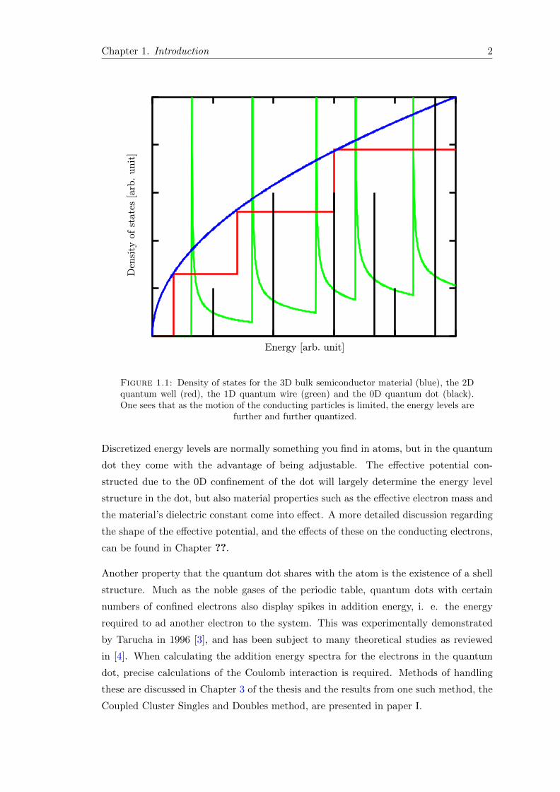
Figure 2.3: Convention for the angles of the magnetic field B.

boundaries of the knot-sequence, the so called numerical box. However these states

are still required and useful to construct the complete and finite basis, a property we

eventually want to be able solve the many-body Hamiltonian in Section 2.2 accurately.

2.1.4 Magnetic Field

We now want to add a general time-independent magnetic field potential to the dot.

The most trivial magnetic field is one lying in the z-direction, however we chose a more

general field:

B = B0 (cosφsinθ, sinφsinθ, cosθ) , (2.17)

giving us the vector potential:

A =B0

2(z cosφ sin θ − y cos θ, x cos θ − z sinφ sin θ, y sinφ sin θ − x cosφ sin θ) , (2.18)

In our convention θ is the inclination angle and φ is the azimuthal angle from the x-axis,

as seen in figure 2.3. The Hamiltonian in equation 2.1 can be rewritten:

hop =p2

2m∗+ V (x) +

e2

2m∗A2 +

e

2m∗B · L + g∗µbB · S. (2.19)


Now if we assume an almost two-dimensional dot, the contributions in the z-direction

vanish, leaving us with the quadratic coupling:

A2 =B2

0

4

((x2 + y2) cos2 θ + sin2 θ(y sinφ− x cosφ)2

), (2.20)

the linear coupling:

B · L = B0 cos θLz (2.21)

and the spin coupling:

g∗µbB · S = g∗µbB0 cos θsz. (2.22)

The quadratic term will act as a anisotropic two-dimensional harmonic potential, where

the angles θ and φ will control the direction of the anisotropy. This is easily seen by

fixing φ to zero and ending up with the potential:

A2 =B2

0

4

(x2 + y2 cos2 θ

), (2.23)

where the harmonic potential in the y-direction is dampened by a factor cos θ. With a

general azimuthal angle φ an equivalent elliptical potential is created but with its axis

in the direction of φ. So for a tilted magnetic field the dominating effect will be that of

an anisotropic harmonic oscillator potential with its axis in the φ-direction.

A Cartesian basis will be more natural to use when a tilted magnetic filed is involved,

since the quadratic magnetic effect only has a cylindrical symmetry in the case when θ is

zero. The first part of eq. 2.20 is separable and can be added to the two one-dimensional

Schrodinger equations (2.9). The second part of eq. 2.20 and the linear magnetic term

both mix in the x-y-dimensions and need to be added separately, mixing the states

produced in subsection 2.1.2.


2.2 Many-Body Treatment

In the previous section a single-particle basis has been created, which we may now use

in an attempt to solve the many-body Hamiltonian:

HMB =

N∑i

hi +

N∑i<j

e2

4πεε0 |ri − rj |(2.24)

Here we have separated the Hamiltonian into two parts, the non-interacting, one-body

part, hi that we have already solved, and the many-body, electron-electron interaction.

Some of the simpler methods used to do solve this problem are so called mean-field

methods, where the electron-electron interaction is simplified to a one-body interaction

with a total potential created by all the other electrons collectively. Hartree-Fock (HF)

and Density Function Theory (DFT) are two such methods, but both lack accuracy to

one degree or the other. HF does not include any correlation effects and will be a fairly

bad method when we increase our number of particles. DFT can produce very high

quality results, but they are dependent on the functionals used and the accuracy of the

method is hard to determine beforehand.

In this work, focus is on more exact numerical many-body methods; Configuration

Interaction (CI), Many-Body Perturbation Theory (MBPT) and Coupled Cluster (CC).

To start out we should define some things. First off a many-body wave function for a

system consisting of N electrons can be written as a product of single-body functions as

a slater determinant:

Ψ0 = |ψa · ψb · ... · ψN | . (2.25)

So the wave function in eq. 2.25 is a N-electron wave function where the orbitals a, b, ...N

are occupied. We also divide the space constructed by the one-electron states into

two parts, the model space and the function space. The model space is spanned by

model functions, which are states used as starting-points in our numerical routines when

searching for exact many-body wave functions. These are approximations of the exact

wave functions, and the choice of these will be discussed in further detail below. The

function space is the complementary space to the model space, spanned by all the other

wave functions created using our one-body states.


We use the convention of denoting electron orbitals occupied in the model space with the

letters a, b, c, ... and orbitals unoccupied in the model space using the letters r, s, t, ....

When describing a general case where an orbital may be either occupied or unoccupied

the letters m,n, o, ... will be used. A many-body state in the function space, where the

electron occupying the orbital a in the model space, is instead occupying the excited

orbital r, is written as the slater determinant:

Ψra = |ψr · ψb · ... · ψN | . (2.26)

Due to the completeness of the basis, any state, such as the solution the many-body

Hamiltonian in eq. 2.24, can be written as:

Ψ = c0Ψ0 +∑ar

craΨra +

∑abrs

crsabΨrsab +

∑abcrst

crstabcΨrstabc + ... =

∑i

Ψi (2.27)

So the exact many-body state can be written as a superposition of states in our model

and function space. We can see the different parts as the original non-interacting state

and excitations from this configuration, these excitations may be one-electron, two-

electron or more electron excitations. The division based on the degree of excitation will

be useful later on, but for simplicity it is enough to describe them as some excitation

Ψi from Ψ0.

2.2.1 Configuration Interaction

In a similar fashion as previously done when switching basis to the B-spline basis in

subsection 2.1.3, we can now construct an eigenvalue problem on matrix form where we

now search for the coefficients of eq. 2.27.

HC = EC (2.28)


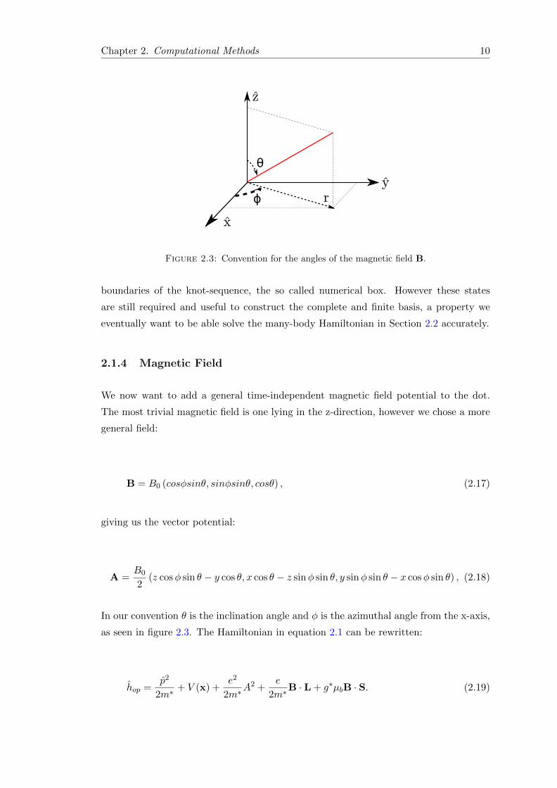
Thanks to the orthogonality of the many-body states in the model and function space. C

will only be a vector containing the coefficients, E will contain the many-body energies

and H is:

H =

〈Ψ0|HMB|Ψ0〉〈Ψ0|HMB|Ψ1〉 . . .

〈Ψ1|HMB|Ψ0〉〈Ψ1|HMB|Ψ1〉 . . ....

.... . .

(2.29)

Using the Configuration Interaction method, one constructs this matrix and diagonalizes

it to form the exact many-body solution to eq. 2.24.

However, this is a very expensive method. Even though we have a finite one-body basis,

the number of many-body functions we can create using these grows very large when

more than a few active electrons are allowed. This usually requires a truncation of some

aspect of the problem, usually by only allowing a certain degree of excitations in the

function space. This is done by removing some of the terms in eq. 2.27, and reducing

the dimensionality of the H-matrix.

But by doing this, certain problems will arise in regards to the solution. The most

obvious is that the complete basis is required to form the exact wave function, however

we must always trade accuracy for speed when using numerical methods, so some loss

in accuracy can be acceptable. A less obvious drawback is lack of size consistency, [12],

that is, truncated CI does not conserve energy when dividing something into several

separate subsystems, [13]. Since we will study potentials with some degree of separation

later on, this may be important. So the only CI used will be non-truncated, Full CI

(FCI).

The matrix-elements of H will consist of the one-electron Hamiltonians from the previous

section and the electron-electron interaction. Since the many-body wave functions are

eigenstates to the sum of one-electron Hamiltonians, this part falls out into a diagonal

matrix.

The non trivial part that is left is the ee-interaction:

〈Ψk|N∑i<j

e2

4πεε0 |ri − rj ||Ψl〉 (2.30)


The electron-electron interaction is actually a two particle operator, so the matrix ele-

ment will be a sum of all possible two-particle combinations belonging to the states Ψk

and Ψl such as:

〈op|k1

r12|mn〉l, (2.31)

where particles op belong to state k and particles mn belong to state l. Depending on

the configuration of the one-particle states, these 1/r12 matrix elements will be added

with different signs, or may be zero.

When using the polar solutions to the one-body Hamiltonians we can use the expansion

suggested by Cohl et al. in [14] and write the 1/r12 matrix elements as:

〈op| 1

r12|mn〉 =

e2

4πεrε0

ml=∞∑ml=−∞

〈uo(r1), up(r2)|Qml−1/2(ξ)

π√r1r2

|um(r1), un(r2)〉

·〈eimol φ1eim

pl φ2 |eiml(φ1−φ2)|eimm

l φ1eimnl φ2〉〈mo

s|mms 〉〈mp

s|mns 〉.

(2.32)

Here the numbers 1 and 2 denote the first and second particle, uo(r), m and the ms

quantum numbers are defined as in eq. 2.5. The Qml−1/2(ξ) functions are Legendre

functions of the the second kind and half integer degree solved using software from

[15]. Thanks to the use of B-splines, the radial integrals that need to be evaluated are

polynomial, allowing the use of exact Gaussian integration. The angular integrals will

only be non-zero given certain quantum numbers, leading us to some selection-rules,

namely: mol −mm

l = ml = mpl −m

nl , mo

s = mms and mp

s = mns .

In the case of Cartesian coordinates the process is more straight forward however special

care must be taken when operating close to the poles in the 1/r12 operator, to circumvent

division by zero.

2.2.2 Perturbation Theory

Moving on to the many-body perturbation theory, the idea is to perturbativly add the

ee-interaction to an already known solution. This presents a number of options on what

to do and the work done here is based on Lindgren and Morrisons textbook on many-

body atomic physics, [16]. The goal is to achieve a perturbation expansion to all order,

that is including all possible linked Coulomb interactions. If electron pair a and b couple


to pair r and s, we should also include the effect from the subsequent coupling r and

s to all other pairs. In CI this is included in the diagonalization of the Hamiltonian

matrix, and therefore all interactions are included. With perturbation theory we hope

to achieve the same thing without the computational expens of FCI or the drawbacks

of truncated CI.

To start of we want to divide the complete Hamiltonian into two parts, H = H0 + V ,

with the exact unknown eigenstate Ψ. Here H0 has a known solution Ψ0 that is an

approximation of Ψ, and V is treated as a perturbation to H0. We have the option to

either place the entire electron-electron interaction in V or place some of it in H0 by

first using something simpler, such as the Hartree-Fock method that includes some, but

not all ee-effects. Hence, V becomes:

V =∑

i<j≤N

1

rij−∑i≤N

ui, (2.33)

where ui is some one-particle potential already included in the solution of H0. The

reason to do this is to possibly include some of the ee-interaction in the model function,

by using solutions from some mean-field method, such as Hartree-Fock. This will not

effect the solution since all interactions are included in the MBPT method but may

speed up the process.

In the previous subsection, the concept of model-space and function-space have already

been defined. The model space may span any number of many-body functions, but

for simplicity we start of by investigating the case where it only contains one model

function |Ψ0〉. It becomes useful to create some projection-operators associated to these

spaces, P = |Ψ0〉〈Ψ0| which projects onto the model function, and Q =∑

β 6=Ψ0|β〉〈β|

which projects onto the complimentary functions. The two projection operators form a

complete space, i.e. P +Q = 1. We also chose to normalize our functions in such a way

that 〈Ψ0|Ψ〉 = 1. This allows us to write the exact solution as the model function plus

a correction in function space:

|Ψ〉 = (P +Q)|Ψ〉 = |Ψ0〉+Q|Ψ〉 (2.34)

Finally we define the wave operator Ω and the correlation operator χ. The wave operator

has the property that it creates the exact state when operating on the model function,

i.e. Ω|Ψ0〉 = |Ψ〉. The correlation operator is defined by Ω = 1 + χ, and will when


operating on the model function, create the correction in function space to the model

function:

χ|Ψ0〉 = (Ω− 1)|Ψ0〉 = |Ψ〉 −P |Ψ〉 = |Ψ0〉+Q|Ψ〉 − |Ψ0〉 = Q|Ψ〉 = QΩ|Ψ0〉 (2.35)

We can now rewrite the Schrodinger equation onto a, for the purpose, more useful form

called the Bloch equation, formulated in [17]. The SE in our operator form reads:

H|Ψ〉 = H0|Ψ〉+ V |Ψ〉 = E|Ψ〉, (2.36)

or

(E −H0)|Ψ〉 = V |Ψ〉, (2.37)

we now project onto our model space using the P operator, which commutes with H0

since Ψ0 is an eigenfunction.

P (E −H0)|Ψ〉 = (E −H0)|Ψ0〉 = PV |Ψ〉. (2.38)

Next step is to use the definition of the wave operator:

P (E −H0)|Ψ〉 = E|Ψ0〉 −H0|Ψ0〉 = PV Ω|Ψ0〉, (2.39)

and then operate with Ω:

EΩ|Ψ0〉 − ΩH0|Ψ0〉 = E|Ψ〉 − ΩH0|Ψ0〉 = ΩPV Ω|Ψ0〉. (2.40)


We now replace E|Ψ〉 with the SE in eq. 2.36 and once again use the definition of the

wave operator:

E|Ψ〉−ΩH0|Ψ0〉 = (H0+V )|Ψ〉−ΩH0|Ψ0〉 = (H0+V )Ω|Ψ0〉−ΩH0|Ψ0〉 = ΩPV Ω|Ψ0〉,

(2.41)

and by shuffling the terms we get:

H0Ω|Ψ0〉 − ΩH0|Ψ0〉 = ΩPV Ω|Ψ0〉 − V Ω|Ψ0〉. (2.42)

We bring in a 〈Ψ0| from the right and switch signs to write this with a commutator on

the form:

[Ω, H0]P = V ΩP − ΩPV ΩP. (2.43)

Finally we want to use a formalism where we create excitations from the model space

P onto the function space Q, therefor we use our definition of χ to rewrite this onto its

final form, the Bloch equation:

[Ω, H0]P = QV ΩP − χPV ΩP. (2.44)

We can now divide the wave operator order by order, Ω = 1 + Ω1 + Ω2 + ..., and likewise

for the correlation operator, χ = Ω1 + Ω2 + .... Here the order of the operator denotes

the number of ee-interactions involved in the operator. The point of this is to create

an order-by-order scheme to construct our wave operator, so by inserting the expanded

operator into the Bloch equation we may identify connections between different parts of

the two sides of the equation:

[(1 + Ω1 + ...), H0]P = QV (1 + Ω1 + ...)P − (Ω1 + ...)PV (1 + Ω1 + ...)P (2.45)


[1, H0]P = 0

[Ω1, H0] = QV P

[Ω2, H0] = QV Ω1P − Ω1PV P

[Ω3, H0] = QV Ω2P − Ω2PV P − Ω1PV Ω1P

...

(2.46)

By calculating all the matrix elements QV P we can now create the first order wave

operator, and by using Ω1 we can continue constructing Ω2 and so on. When evaluating

the operators, certain parts of the right hand side of the expressions may be found to

have so called unlinked or disconnected parts. These are called the unlinked diagrams

when applying a diagrammatic approach to the problem.

The clearest case are of the variety Ω2PV P , here the V operator operates between the

model functions only creating an energy contribution of the form of a constant number.

Also the Ω1PV Ω1P term has a similar closed off part, here created by the Ω1 and

subsequent V operator, creating another energy contribution. If the QV Ω2P term is

expanded, the same parts with the same closed of energy contribution will be found,

but only if we allow for the Pauli exclusion principle to be violated. That is, we allow

for unphysical states where several particles are allowed to occupy the same orbitals at

once. If this is done in all terms of eq. 2.44, we will get a cancellation between the

disconnected parts of first term and the entire second term of the right hand side. This

is called the linked-diagram theorem and details may be found in [16]. This allows us

to formulate the Bloch equation in a new way:

[Ωi, H0]P = (QV Ωi−1P )linked, (2.47)

where only the linked diagrams, but all Pauli principle violating diagrams are included

in the right hand side. Note that the resulting wave operator is not Pauli violating,

these terms are only there to ensure the cancellation of the second term in eq. 2.44.

We now wish to utilize the wave operator expansion to find the exact wave function |Ψ〉and the states energy E. The wave operator has been divided order-by-order, and so


can the wave function:

|Ψ〉 = Ω|Ψ0〉 = |Ψ0〉+ Ω1|Ψ0〉+ Ω2|Ψ0〉+ ... = |Ψ0〉+ χ|Ψ0〉 (2.48)

Now, χ|Ψ0〉 operates from P space to Q space as in eq. 2.35 so we are only interested in

the parts of the wave operator doing the same. If we operate with the Q-operator from

the left-hand side of eq. 2.46, we can investigate the effects on the first order operator:

Q[Ω1, H0] = QΩ1H0P −QH0Ω1P (2.49)

By letting the H0 operator operate to the right on P in the first term and to the left on

Q in the second term, we can replace the H0 operator with its eigenvalues:

QΩ1H0P −QH0Ω1P = QΩ1EPP −QEQΩ1P =

=∑β 6=Ψ0

(|β〉〈β|Ω1ε0|Ψ0〉〈Ψ0| − |β〉〈β|εβΩ1|Ψ0〉〈Ψ0|) =

= (ε0 − εβ)∑β 6=Ψ0

|β〉〈β|Ω1|Ψ0〉〈Ψ0|

(2.50)

If we also rewrite the right hand side of the corresponding row of eq. 2.46, we can express

the first order wave function as:

|Ψ1〉 = QΩ1|Ψ0〉 =∑β 6=Ψ0

|β〉〈β|Ω1|Ψ0〉 =∑β 6=Ψ0

|β〉〈β|V |Ψ0〉(ε0 − εβ)

(2.51)

By doing the same thing for the other lines of eq. 2.46 we now have a way of constructing

the complete wave function, order by order.

To find the corresponding energy we define a effective Hamiltonian, Heff , with the

properties that its eigenvalue is the exact energy E corresponding to the exact wave


function |Ψ〉, and its eigenfunction is the model function |Ψ0〉. To get these properties

the effective Hamiltonian must be defined as follows:

Heff = PHΩP = PH0P + PV ΩP (2.52)

In a similar way to how the wave function was treated, we now divide the energy into

an order-by-order expansion:

〈Ψ0|E|Ψ0〉 = 〈Ψ0|Heff |Ψ0〉 =

= 〈Ψ0|H0|Ψ0〉+ 〈Ψ0|V |Ψ0〉+ 〈Ψ0|V Ω1|Ψ0〉+ 〈Ψ0|V Ω2|Ψ0〉+ ... =

= E0 + E1 + E2 + E3 + ...

(2.53)

Note that the first order wave operator, Ω1, produces the second order energy, E2, since

an additional electron-electron interaction is added to it.

Even though a scheme for finding the true many-body wave function and energy has

been found, it is not a very practical one. Since the different order wave operators can

be combined in more ways to form higher order operators, a computer algorithm will be

tough to construct. A better form would be an iterative equation where one can insert

one iteration of the solution once again into the same equation to form a higher order

solution. Such a Bloch equation would instead be:

[Ω(i), H0]P = QV Ω(i−1)P − χ(i−1)PV Ω(i−1)P, (2.54)

where the starting point wave and correlation operators are Ω(0) = 1 and χ(0) = 0. By

inserting the expressions for Ω iteration by iteration, one would find that the expressions

do not match the order by order formalism in eq. 2.46. However, the sum of the all-order

expansion of wave operators in both formalisms would be the same, i. e. given that

a self consistent solution is reached through iteration, it will be equivalent to the one

found order-by-order.

For an exact solution all orders of the wave operator need to be included, but the

contribution to the energy and wave function will be smaller and smaller for each order as

each higher order operator is built from lower order operators. However, size consistency

once again may play an important roll. It has been shown, [13], that MBPT is only


size consistent if it includes simultaneous pair excitations in the separated subsystems.

These are disconnected quadruple excitations i. e. two separate double excitation in the

subsystems. So if we implement MBPT using the linked diagram theorem, and truncate

it by the double excitations, we will not include these disconnected ”double-double”

excitations. To be sure to include this, we can not truncate the wave function before

the fourth order. But by a slight modification to how we treat the wave operator, we

may include all double excitations, even simultaneous ones we have thus far treated as

quadruple excitations. This treatment is called the Coupled Cluster method.

2.2.3 Coupled Cluster

The Coupled Cluster method (CC), originates from the field of nuclear physics [18],

and has since then been well used in atomic, molecular and chemical physics, see for

instance [19] for a review of the use in these areas. Due to the atom-like properties of

low dimensional semiconductor systems, and the theoretical modeling using an effective

potential, the method has also seen some recent use in this area such as [20–22] and

paper I in this thesis.

We define: SN = ΩN,connected, a cluster operator of order N is defined as the part of the

wave operator that creates excitations of the N :th order, that may not be subdivided

into several disconnected lower order excitations. As an example, a double excitation

from the model function, exciting electrons in orbitals a and b to r and s, 〈Ψrsab|V |Ψ0〉,

is a pure double excitation included in the S2 operator. However two single excitations,

〈Ψsb|V |Ψ0〉〈Ψr

a|V |Ψ0〉, resulting in the same total excitation to the state Ψrsab, will not be

included, but will instead be a case of two single excitations S12. Both of these are

double excitations belonging to the Ω2 operator, but are built by two different classes

of cluster operators.

We can write the entire wave operator as the exponential function of the sum of all

cluster operators:

Ω = eS = eS1+S2+S3+... = 1+S1+S2+1

2!S12+S3+S1S2+

1

3!S13+..., (2.55)

where the curly brackets denote anti-symmetrization of the operators. The right-hand

side of eq. 2.55 can now be subdivided into the different orders of the the wave operator

as follows:


Ω1 = S1

Ω2 = S2 +1

2!S12

Ω3 = S3 + S2S1+1

3!S13

Ω4 = S4 + S3S1+1

2!S22 +

1

2!S2S

21+

1

4!S14

...

(2.56)

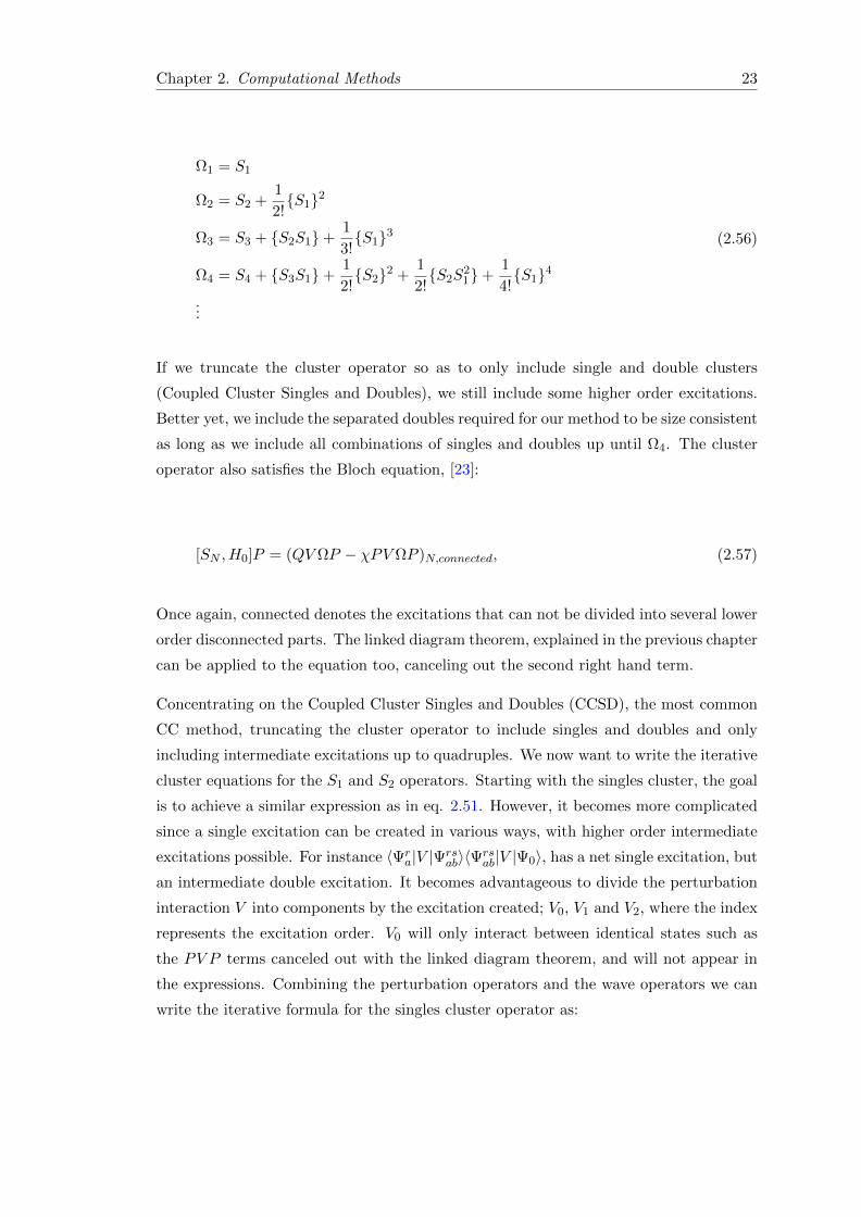
If we truncate the cluster operator so as to only include single and double clusters

(Coupled Cluster Singles and Doubles), we still include some higher order excitations.

Better yet, we include the separated doubles required for our method to be size consistent

as long as we include all combinations of singles and doubles up until Ω4. The cluster

operator also satisfies the Bloch equation, [23]:

[SN , H0]P = (QV ΩP − χPV ΩP )N,connected, (2.57)

Once again, connected denotes the excitations that can not be divided into several lower

order disconnected parts. The linked diagram theorem, explained in the previous chapter

can be applied to the equation too, canceling out the second right hand term.

Concentrating on the Coupled Cluster Singles and Doubles (CCSD), the most common

CC method, truncating the cluster operator to include singles and doubles and only

including intermediate excitations up to quadruples. We now want to write the iterative

cluster equations for the S1 and S2 operators. Starting with the singles cluster, the goal

is to achieve a similar expression as in eq. 2.51. However, it becomes more complicated

since a single excitation can be created in various ways, with higher order intermediate

excitations possible. For instance 〈Ψra|V |Ψrs

ab〉〈Ψrsab|V |Ψ0〉, has a net single excitation, but

an intermediate double excitation. It becomes advantageous to divide the perturbation

interaction V into components by the excitation created; V0, V1 and V2, where the index

represents the excitation order. V0 will only interact between identical states such as

the PV P terms canceled out with the linked diagram theorem, and will not appear in

the expressions. Combining the perturbation operators and the wave operators we can

write the iterative formula for the singles cluster operator as:


〈Ψra|S1|Ψ0〉i+1 =

1

εa − εr〈Ψr

a|V1 + (V1 + V2)S1 + (V1 + V2)S2+

+1

2!(V1 + V2)S12 + V2S1S2+

1

3!V2S13|Ψ0〉i

(2.58)

In the same way the doubles operator expression becomes:

〈Ψrsab|S2|Ψ0〉i+1 =

1

εa + εb − εr − εs〈Ψr

a|V2 + V2S1 + (V1 + V2)S2 +1

2!V2S12+

+ (V1 + V2)S1S2+1

3!V2S13 +

1

2!V2S22 +

1

2!V2S2

1S2+1

4!V2S14|Ψ0〉i

(2.59)

Figuring out the ways to combine the operators to form the different orders of excitations

is in no way a trivial matter, and is the greatest drawback of the CC method. But if

this is done properly and the cluster expressions are implemented in a numerical routine

very high accuracy results may be calculated fairly inexpensively. Such results may be

viewed in comparison to other methods such as the FCI and Quantum Monte Carlo

methods in paper I.

Chapter 3

Effective Potentials

The effective potential is the total interaction the electrons has with the surrounding

material. Depending on the material properties, it may see some different potential

structures. Here we investigate two of these, the quantum dot and the quantum ring,

including some special cases of these to systems.

3.1 Quantum Dot

In chapter 3 several methods capable of handling energy and wave function calculations

on our desired two dimensional semiconductor systems have been presented. We now

change our focus to some specific systems and start with the quantum dot. Two of the

most common models for quantum dots are the harmonic oscillator potential and the

hard wall potential.

The circular two dimensional harmonic oscillator has been shown to be in good agree-

ment for few electron quantum dots in [24], and has already been briefly discussed

previously in this work. It is also the model used in paper I for the high precision results

discussed there. The hard wall and harmonic models are both used in paper II, and are

compared to each other under the influence of a tilted magnetic field. Here, the har-

monic oscillator will be the main focus, and the hard wall will mostly be compared to

the harmonic model. Also the anisotropic, elliptic, harmonic oscillator will be discussed

briefly.

25

Chapter 3. Effective Potentials 26

3.1.1 Harmonic Oscillator

The two dimensional harmonic oscillator potential and the one particle solutions have

already been discussed in subsections 2.1.1 and 2.1.2. Depending on the number of

electrons in the quantum dot we want to use different methods to calculate the many-

body energies.

For two electrons it is fully viable to use the complete one-electron basis constructed with

B-splines to solve the problem with untruncated FCI. Modern computers and algorithms

have very little trouble diagonalizing matrices with thousands of elements, so there is

no real requirement to truncate the basis used in FCI. Due to the completeness of the

basis, and the nature of the FCI method, near exact results should be obtained with

this method. MBPT is also usable for two electrons, and given that it is allowed to

iterate until a self consistent solution is obtained, it should yield the same results as

FCI. CCSD will be identical to MBPT for two particles and is therefor mainly just a

more complicated method that achieves the same results.

We may want to truncate the basis to increase the speed of the calculations and still

achieve adequate results. Size consistency should not be an issue as no separated double

excitations may occur, so both MBPT and FCI can be truncated without loosing any

physical properties. A way to truncate the basis is by the energy of the states. In

MBPT this becomes obvious in eq. 2.51, where the energy difference between the states

in the model space and states in the function space are in the denominator. For FCI this

can be shown by diagonalizing a matrix with only two states, where one will see that

the coupling strength between the states decreases as the energy difference increases.

However, since the two methods give the same results we also know this has to be true.

For more electrons it is possible to use untruncated FCI or MBPT, but due to the scaling

relation of calculation time and the number of particles, this becomes more and more

resource demanding, and will eventually be impossible due to the time and memory it

would require from the computer to run it. Truncating the basis is still an option, but

as can be seen in paper I, the size of the basis is often more important than using an

exact method with respect to the accuracy of the orbital energy. So the better option

for more than four electrons is to change to another method, such as the CCSD. In

paper I, results for CCSD with as many as 12 electrons have been presented with good

accuracy, compared to the FCI and Quantum Monte Carlo. In table 3.1 an outtake

from the article can be seen, showing the comparison between the CCSD routine and

previously published FCI results.

Some basis truncation will most often be needed or at least useful to speed up the

calculations and it has already been declared that the energy of the one-particle states


Table 3.1: Comparison between the Coupled Cluster Singles and Doubles method andFull Configuration Interaction according to Kvaal [25–27] and Rontani [28]. The basisis in all three cases defined by the one-electron harmonic oscillator Hamiltonian and istruncated after a specific number of major oscillator shells R = 2n+ |ml|. Energies are

given in units of ~ω and the number of confined electrons is 2-6 and 8.

CCSD FCI|2S ML〉 ~ω(meV ) Basis set This work Kvaal Rontani et al.

N=2 |00〉 11.85720 R=7 3.009234 3.0092362.964301 R=7 3.729323 3.729324 3.72950.3293668 R=5 5.784651 5.78500.1852688 R=7 6.618089 6.6185

N=3 |11〉 11.85720 R=10 6.36773 6.3656152.964301 R=7 8.17635 8.166708 8.1671

N=4 |20〉 2.964301 R=7 13.635 13.626

N=5 |11〉 2.964301 R=7 20.3467 20.33

N=6 |00〉 2.964301 R=5 28.0161 28.0330 28.03R=7 27.9751 27.98R=15 27.9390

N=8 |20〉 2.964301 R=5 47.13801 47.14R=15 46.67960

is a natural method of doing this. The one electron energies for the Cartesian and polar

solutions: εnx,ny = (nx + ny + 1)~ω and εnml= (2n + |ml| + 1)~ω, will yield identical

results and degeneracies, so cutting at the same energy using the different methods will

result in the same basis truncation. The polar one-electron energies can be seen plotted

in figure 3.1. By observing the energy structure, we introduce a new compound quantum

number R = 2n + |ml|. R scales with energy, so a truncation by R will ensure that all

states of the energy E ≤ (R+1)~ω will be included in the basis. The Cartesian energies

may be mapped to the polar states and truncated in the same way with the same results.

More complex truncation methods can be devised and implemented to ensure that only

states with important contributions are included, but will require some prior knowledge

about the solution.

With R we have also found a possible shell-structure in the many-body energies. The

idea behind a shell-structure, is inspired by the structure found in atoms. Assuming the

non-interacting many-body energy is close to the final many-body energy with the ee-

interactions included, one expects the addition energy to spike at 3, 7 and 13 electrons.

The addition energy is the extra energy contribution a system requires to bind a new

particle to it. These numbers come from figure 3.1 where each bar in the figure is capable

of storing two electrons (one spin up and one spin down). So if the first two electrons

are placed in the lowest energy states, the next electron to be added will need to be

placed in a state of higher energy than the previous two. The same thing occurs again

when the next two levels are filled, requiring the 7:th electron to have a higher energy.


ml

En=1

n=0...

0 1 2 3-1-2-3

Figure 3.1: The one particle energies states of the quantum dot and their corre-sponding quantum numbers. In the x-axis the ml quantum number is increased anddecreased, with the n quantum number being constant in each marked ”V”, and the

energy increases along the y-axis.

If the electron-electron interaction eventually starts to dominate over the basis energy

structure, some changes to the structure may occur. However studies show that the

three lowest shells (2, 6 and 12 electrons) indeed seem to follow what is expected from

the one-electron basis, [29].

3.1.2 Elliptic Harmonic Oscillator

The elliptic harmonic oscillator (EHO) has the potential shape: V (x, y) = 12m∗ω2(δx2 +

(1/δ)y2). Since the EHO lacks cylindrical symmetry but is still parabolic in both the

x and y-dimensions, the Cartesian coordinates solution may be used after scaling the

potential strength in the x and y direction. The effects of the dots ellipticity has been

studied somewhat before, [30–32], and even small elliptic effects have been shown to

alter the shell structure noticeably.

In paper II this is of importance since a tilted magnetic field is applied to a two electron

dot. The tilted field in itself will have a quadratic term that acts as an elliptic harmonic

potential in the φ direction as seen in section 2.1.4. In paper II, experimental results

are compared to results from a CI routine for both hard wall and harmonic potentials.

The hard walls ellipticity is added as an extra harmonic perturbation in one dimension,

εx2, to the the potential described in section 3.1.3.

Further studies of the EHO dot with a tilted magnetic field has led to some further

understanding of the different parameters. As in paper II, the energy splitting between

the lowest lying singlet and triplet states are investigated. As the magnetic field is

increased, these two states will eventually cross and the triplet state will become the


ground state. Figures 3.2, 3.3 and 3.4 show the experimental data from [5] and the

results from CI calculations with different sets of parameters.

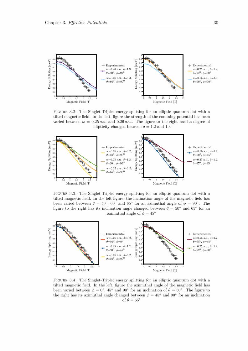
In figure 3.2 we see the effects of the dot parameters, i.e. the oscillator strength and

ellipticity. In the left figure the oscillator strengths is varied with the result of translating

the curve, increasing the splitting with higher oscillator strengths. This increase in

splitting is however only valid for sufficiently large oscillator strengths, eventually non-

linear energy contribution terms may start to dominate changing this behavior. The

other figure shows the effect of the ellipticity, the energy splitting with no magnetic

field is decreased with a higher degree of ellipticity, while the splitting at higher field

strengths remains the same. The result of this is a small plateau at low magnetic fields,

that is wider for more elliptic dots.

Figure 3.3 displays the effect the inclination angle has. In the left figure the azimuthal

angle is perpendicular to the ellipticity, φ = 90, and in the right figure this angle is

45. The two angular parameters are naturally of no importance at zero magnetic field

and will determine the slope of the curve for higher fields. A large inclination angle will

reduce the magnetic fields z-component, thereby also reducing most of the fields effect

on the energy, flattening the curve. This effect is seen in both figures, where the slope

is flatter in the 65 case than for 50.

The last figure, 3.4, shows the effect of the azimuthal angle, i.e. the difference in orien-

tation between the magnetic field and the ellipticity of the dot. The left graph shows

an inclination angle of 50 and the right graph 65. Once again the effect of the angle

grows in importance with the strength of the magnetic field, by changing the slope of

the curve. This effect is more prominent for larger inclination angles, and once again the

reason is the importance of the B-field z-component. The components of the field not

in the z-direction make the magnetic field interaction elliptical, and this effect is com-

peting against the elliptic form of the dot. Depending on the difference in orientation

the magnetic field may either enhance the elliptical form, or weaken it. With a strong

field, this effect is of less importance, making the curve in the graphs less sensitive to

the angle.

The experimental data has an inclination angle of θ = 68 ± 5 with an unknown az-

imuthal orientation and ellipticity. In paper II, good agreement was not found for the

harmonic oscillator dot with no azimuthal angle. However with a new implementa-

tion we now have the possibility of investigating the different parameters, including the

azimuthal angle in more detail.


0 0.5 1 1.5 2 2.5 30

0.1

0.2

0.3

0.4

0.5

0.6

0.7

0.8

0.9

1

Experimental

Ener

gy S

plitt

ing [m

eV]

Magnetic Field [T]

w=0.25 a.u., ±=1.3,

µ=60o, Á=90o

Experimental

Ener

gy S

plitt

ing [m

eV]

Magnetic Field [T]

w=0.2616 a.u., ±=1.3,

µ=60o, Á=90o

w=0.25 a.u., ±=1.3,

µ=60o, Á=90o

0 0.5 1 1.5 2 2.5 30

0.1

0.2

0.3

0.4

0.5

0.6

0.7

0.8

0.9

1

0.4

0.5

0.6

0.7

0.8

0.9

1

Experimental

Ener

gy S

plitt

ing [m

eV]

Magnetic Field [T]

w=0.25 a.u., ±=1.2,

µ=60o, Á=90o

w=0.25 a.u., ±=1.3,

µ=60o, Á=90o

w=0.26 a.u., ±=1.3,

µ=60o, Á=90o

Figure 3.2: The Singlet-Triplet energy splitting for an elliptic quantum dot with atilted magnetic field. In the left, figure the strength of the confining potential has beenvaried between ω = 0.25 a.u. and 0.26 a.u.. The figure to the right has its degree of

ellipticity changed between δ = 1.2 and 1.3

0 0.5 1 1.5 2 2.5 30

0.1

0.2

0.3

0.4

0.5

0.6

0.7

0.8

0.9

1

Experimental

Ener

gy S

plitt

ing [m

eV]

Magnetic Field [T]

w=0.25 a.u., ±=1.2,

µ=50o, Á=90o

w=0.25 a.u., ±=1.2,

µ=60o, Á=90o

w=0.25 a.u., ±=1.2,

µ=65o, Á=90o

ExperimentalE

ner

gy S

plitt

ing [m

eV]

Magnetic Field [T]

w=0.2616 a.u., ±=1.3,

µ=60o, Á=90o

w=0.25 a.u., ±=1.3,

µ=60o, Á=90o

Experimental

w=0.25 a.u., ±=1.2,

µ=50o, Á=45o

w=0.25 a.u., ±=1.2,

µ=65o, Á=45o

0 0.5 1 1.5 2 2.5 30

0.1

0.2

0.3

0.4

0.5

0.6

0.7

0.8

0.9

1

0.4

0.5

0.6

0.7

0.8

0.9

1

Ener

gy S

plitt

ing [m

eV]

Magnetic Field [T]

Figure 3.3: The Singlet-Triplet energy splitting for an elliptic quantum dot with atilted magnetic field. In the left figure, the inclination angle of the magnetic field hasbeen varied between θ = 50, 60 and 65 for an azimuthal angle of φ = 90. Thefigure to the right has its inclination angle changed between θ = 50 and 65 for an

azimuthal angle of φ = 45

0 0.5 1 1.5 2 2.5 30

0.1

0.2

0.3

0.4

0.5

0.6

0.7

0.8

0.9

1

Experimental

Ener

gy S

plitt

ing [m

eV]

w=0.25 a.u., ±=1.2,

µ=50o, Á=0o

w=0.25 a.u., ±=1.2,

µ=50o, Á=45o

w=0.25 a.u., ±=1.2,

µ=50o, Á=90o

Magnetic Field [T]

Experimental

Ener

gy S

plitt

ing [m

eV]

Magnetic Field [T]

w=0.2616 a.u.,

µ=60o, Á=90

w=0.25 a.u.,

µ=60o, Á=90

Experimental

w=0.25 a.u., ±=1.2,

µ=65o, Á=45o

w=0.25 a.u., ±=1.2,

µ=65o, Á=90o

0 0.5 1 1.5 2 2.5 30

0.1

0.2

0.3

0.4

0.5

0.6

0.7

0.8

0.9

1

0.4

0.5

0.6

0.7

0.8

0.9

1

Ener

gy S

plitt

ing [m

eV]

Magnetic Field [T]

Figure 3.4: The Singlet-Triplet energy splitting for an elliptic quantum dot with atilted magnetic field. In the left, figure the azimuthal angle of the magnetic field hasbeen varied between φ = 0, 45 and 90 for an inclination of θ = 50. The figure tothe right has its azimuthal angle changed between φ = 45 and 90 for an inclination

of θ = 65


3.1.3 Hard Wall

The results in paper II indicate that there may be a significant difference in using a hard

wall (HW) or harmonic (HO) model to describe some QD systems. Due to this result

the hard wall dot model will be discussed shortly.

The circular hard wall is written:

V (r) =

0 ; r < r0

∞ ; r ≥ r0

(3.1)

An alternative to this is to use an anharmonic potential of the form:

V (r) =

(r

r0

)2n

, (3.2)

where n is a number larger than 1. In the limit of n → ∞, this will be identical to the

potential described above, but will be sufficiently ”hard” for lower n:s. This is a more

useful form when using a Cartesian basis where an ellipticity may be added as:

V (x, y) =

(δx2 + 1/δy2

)nr2n

0

, (3.3)

The HW potential has analytical one-particle solutions, but it can also be solved using

B-splines. The wave functions and energies are similar to the ones found solving the

radial 2D harmonic oscillator potential. The main difference is the radial distribution.

Due to the infinite walls in the circular HW potential the electrons wave functions will

be strictly constrained within the limit of r0. In the HO case on the other hand, no

such limitations exist, and high energy states may have their wave functions spread out

over a much larger area. This stronger confinement on the hard wall wave functions will

increase the effect of the electron-electron interaction strength. As this interaction is

controlled by the factor 1|r1−r2| in the denominator, the proximity of the states will be

very important. As seen in paper II, there is some difference in the singlet-triplet energy

splitting between the HW and HO models.


ml

En=1

n=0

...

0 1 2 3-1-2-3

Figure 3.5: The one particle energies states of the quantum dot-ring transition andtheir corresponding quantum numbers. In the x-axis the ml quantum number is in-creased and decreased, with the n quantum number being constant in each marked ”V”,and the energy increases along the y-axis. The dashed lines belong to the quantum dotstates and the full lines to a quantum ring. The finely dotted lines are the states in a

ring with an infinite radius.

3.2 Quantum Ring

The Quantum Ring (QR) can just as the quantum dot, be modeled in several ways.

Using a harmonic oscillator form, one can write it in polar coordinates as: V (r) =12m∗~ω2(r − r0)2. It then simply takes the shape of a radially displaced harmonic

oscillator rotated around the z-axis. The limit of the QR, when r0 → ∞, will be the

infinite one-dimensional quantum wire. The solutions to this is known, and the wave

functions will be plane waves in the φ-dimension and harmonic oscillator solutions in

the r-dimension. Given this, we expect our one-particle ring solutions with the same

radial, n-quantum number, to become more and more degenerate when r0 is increased.

Using the same type of illustration as in section 3.1.1, figure 3.5 visualizes this.

The energy of the ml states decrease, resulting in the filling of states with higher angular

momenta before the states with a different radial distribution. This will result in an

increased level of degeneracy in the many-body states, which is a potential problem when

using our perturbative methods since the energy difference appears in the denominator.

To counteract this, an extended model space needs to be used, including all degenerate

and nearly degenerate interacting states in the model space. Special measures need to

be taken when using an extended model space, the details of which will not be included

in this work.


Figure 3.6: A double concentric ring illustration, modeled using Gaussian distribu-tions. The top part of the figure shows the radial distribution and the bottom part

shows the 2D distribution of the rotated radial potential.

3.2.1 Concentric Rings

Recently more complex ring-like structures have been experimentally created, such as

the concentric rings by Mano, [8]. Concentric rings are several QR:s that share the same

center. The rings created by Mano are Double Concentric Quantum Rings (DCQR), and

have been modeled as two bell-curves rotated around the z-dimension in other theoretical

studies of the system, [33]. Using such a model, the potential will be:

V (r) = Vi exp

[−(r −RiWi

)2]

+ Vo exp

[−(r −RoWo

)2], (3.4)

where Vi,o, Ri,o and Wi,o are the potential depth, ring radius and ring width of the inner

and outer rings. These parameters have been determined for the experimental system,

but can for the sake of modeling be set freely. Figure 3.6 shows an illustration of such

concentric ring potential.

Filling the rings with electrons is a complicated process. Whether the outer or inner

ring is the favorable, or if the electron wave function will be distributed in both rings

is dependent on the ring parameters and the number of electrons. The outer ring dis-

tributes the electrons over a larger area, reducing the importance of the electron-electron

interaction, but angular momentum is higher. While the smaller ring has the opposite

properties. So every electron added must be distributed favorable between the rings to

minimize the energy. The high variability of the system can allow the shell structure of

the electrons to be engineered in various ways as well as creating highly correlated few


electron states, with a potential of being used when constructing quantum computing

qbits. But as in the case of the single QR this implies degeneracy or near degeneracy of

several states, that will require the use of an extended model space when perturbation

theory is used.

Chapter 4

Outlook

4.1 Outlook

Some work on the elliptical two electron quantum dot remains, the experimental data

still purposes a larger angle than found when using the harmonic oscillator, and a larger

radius for the hard wall case. New results are pointing in the right direction and some

further fitting of the parameters will hopefully be able to give better agreement with the

experiment. After confirming that theory and experimental results match, a scheme for

determining the oscillator ellipticity for an experimental dot will be worked on. Given

the different results in different azimuthal angles, one should be able to determine in

what direction and by how much a dot is elliptic by applying a rotating magnetic field

to it.

The rings and concentric rings have a good one-electron basis developed, and solving

the many-body problem for two electrons is possible with existing code. To go beyond

this CCSD with an extended model space needs to be implemented. With a many

body solution there are many interesting properties to be investigated; shell-structure,

coherent states and excited state lifetimes to name a few. Thanks to the methods ability

to give the many-body energies and wave functions with a high accuracy, these properties

can all be determined and compared to experimental data for validation.

35

Acknowledgements

I would like to start of by thanking the everyone at the atomic physics division for the

nice working environment and all the good fredagsfika.

Special thanks go to my co-workers Marcus and Tor for our joint effort in learning

many-body physics and Fortran programing, as well as the fun game/beer/sausage-

evenings. Also my predecessor Erik Waltersson deserves some extra thanks for laying

the groundwork for what i continued on.

And lots of thanks to my supervisor Eva for teaching us all the physics and Fortran skills

needed to get any of this work done and the great opportunity to become acquainted to

the entire ”Nordforsk group”.

Thanks to Esa Rasanen and his group to for all the nano-knowledge and the many great

visits to Finland. Also big thanks to Jan-Petter Hansen and the Bergen group for the

collaboration on paper 2 and the great time at the Jukola relay.

Lots of thanks to my family and friends for everything. And finally∞-thanks to Cecilia

(+1) for all the support and love needed and supplied, always!

36

Bibliography

[1] H. Ibach and H. Luth. Solid-State Physics, An Introduction to Principles of Mate-

rials Science. Springer-Verlag Berlin Heidelberg New York, 2003.

[2] M. A. Reed, J. N. Randall, R. J. Aggarwal, R. J. Matyi, T. M. Moore, and A. E.

Wetsel. Observation of discrete electronic states in a zero-dimensional semiconduc-

tor nanostructure. Phys. Rev. Lett., 60:535, 1988.

[3] S. Tarucha, D.G. Austing, T. Honda, R.J. van der Hage, and L.P. Kouwenhoven.

Shell filling and spin effects in a few electron quantum dot. Phys. Rev. Lett., 77:

3613, 1996.

[4] S. M. Reimann, M. Koskinen, J. Kolehmainen, M. Manninen, D.G. Austing, and

S. Tarucha. Electronic and magnetic structures of artificial atoms. Eur. Phys. J.

D, 9:105, 1999.

[5] T. Meunier, I.T. Vink, L.H. Willems van Beveren, K.-J. Tielrooij, R. Hanson, F.H.L.

Koppens, H.P. Tranitz, W. Wegscheider, L.P. Kouwenhoven, and L.M.K. Vander-

sypen. Experimental signature of phonon-mediated spin relaxation in a two-electron

quantum dot. Phys. Rev. Lett., 98:126601, 2007.

[6] J. M. Garca, G. Medeiros-Ribeiro, K. Schmidt, T. Ngo, J. L. Feng, A. Lorke,

J. Kotthaus, and P. M. Petroff. Intermixing and shape changes during the formation

of inas self-assembled quantum dots. Appl. Phys. Lett., 71:2014, 1997.

[7] Axel Lorke, R. Johannes Luyken, Alexander O. Govorov, Jorg P. Kotthaus, J. M.

Garcia, and P. M. Petroff. Spectroscopy of nanoscopic semiconductor rings. Phys.

Rev. Lett., 84:2223, 2000.

[8] Takaaki Mano, Takashi Kuroda, Stefano Sanguinetti, Tetsuyuki Ochiai, Takahiro

Tateno, Jongsu Kim, Takeshi Noda, Mitsuo Kawabe, Kazuaki Sakoda, Giyuu Kido,

and Nobuyuki Koguchi. Self-assembly of concentric quantum double rings. Nano

Letters.

[9] T. D. Ladd, F. Jelezko, R. Laflamme, Y. Nakamura, C. Monroe, and J. L. O/’Brien.

Quantum computers. Nature, 464:45, 2010.

37

Bibliography 38

[10] John S. Townsend. A modern approach to quantum mechanics. University science

Books, 2000.

[11] H. Bachau, E. Cormier, P. Decleva, J. E. Hansen, and F. Martin. Rep. Prog. Phys.,

64:1815, 2001.

[12] J. A. Pople, J. S. Binkley, and R. Seeger. Theoretical models incorporating electron

correlation. Int. J. Quantum Chem., 10:1, 1976.

[13] R. J. Bartlett and G. D. Purvis. Many-body perturbation theory, coupled-pair

many-electron theory, and the importance of quadruple excitations for the correla-

tion problem. Int. J. Quantum Chem., 14:561, 1979.

[14] Howard S. Cohl, A. R. P. Rau, Joel E. Tohline, Danan A. Browne, John E. Cazes,

and Eric I. Barnes. Useful alternative to the multipole expansion of 1/r potentials.

Phys. Rev. A, 64:052509, 2001.

[15] J. Segura and A. Gil. Evaluation of toroidal harmonics. Comp. Phys. Comm., 124:

104–122, 1999.

[16] I. Lindgren and J. Morrison. Atomic Many-Body Theory. Series on Atoms and

Plasmas. Springer-Verlag, New York Berlin Heidelberg, second edition, 1986.

[17] C. Bloch. Nucl. Phys., 6:329, 1958.

[18] F. Coester and H. Kummel. Short range correlation in nuclear wave functions.

Nuclear Physics, 17:477–485, 1960.

[19] Rodney J. Bartlett and Monika Musia l. Coupled-cluster theory in quantum chem-

istry. Rev. Mod. Phys., 79(1):291–352, Feb 2007. doi: 10.1103/RevModPhys.79.291.

[20] Thomas M. Henderson, Keith Runge, and Rodney J. Bartlett. Electron correlation

in artificial atoms. Chemical Physics Letters, 337(1-3):138–142, 2001. doi: DOI:

10.1016/S0009-2614(01)00157-9.

[21] Ideh Heidari, Sourav Pal, B. S. Pujari2, and D. G. Kanhere. Electronic structure of

spherical quantum dots using coupled cluster method. J. Chem. Phys, 127:114708,

2007.

[22] M. Pedersen Lohne, G. Hagen, M. Hjorth-Jensen, S. Kvaal, and F. Pederiva. Ab

initio computation of the energies of circular quantum dots. Phys. Rev. B, 84:

115302, 2011.

[23] I. Lindgren. A coupled-cluster approach to the many-body perturbation theory for

open-shell systems. Int. J. Q. Chem. S, 12:33–58, 1978.

Bibliography 39

[24] A. Kumar, S. E. Laux, and F. Stern. Electron states in a gaas quantum dot in a

magnetic field. Phys. Rev. B, 42:5166, 1990.

[25] Simen Kvaal. Harmonic oscillator eigenfunction expansions, quantum dots, and ef-

fective interactions. Phys. Rev. B, 80(4):045321, Jul 2009. doi: 10.1103/PhysRevB.

80.045321.

[26] Sime Kvaal. Priv. Comm. The results are produced using the same software as in

Ref. [25], 2009.

[27] Patrick Merlot. Many–body approaches to quantum dots. Master Thesis,

http://folk.uio.no/patrime/src/master.php. CI-results are produced using the soft-

ware written by Kvaal [25], 2009.

[28] Massimo Rontani, Carlo Cavazzoni, Devis Bellucci, and Guido Goldoni. Full con-

figuration interaction approach to the few-electron problem in artificial atoms. J.

Chem. Phys., 124:124102, 2006.

[29] S. M. Reimann and M. Manninen. Electronic structure of quantum dots. Rev. Mod.

Phys., 74:1283, 2002.

[30] Seigo Tarucha, David Guy Austing, Takashi Honda, Rob van der Hage, and Leonar-

dus Petrus Kouwenhoven. Atomic-like properties of semiconductor quantum dots.

Jpn. J. Appl. Phys., 36:3917, 1997.

[31] S. Sasaki, D. G. Austing, and S. Tarucha. Spin states in circular and elliptical

quantum dots. Physica B, 256-258:157, 1999.

[32] D. G. Austing, S. Sasaki, S. Tarucha, S. M. Reimann, M. Koskinen, and M. Man-

ninen. Ellipsoidal deformation of vertical quantum dots. Phys. Rev. B, 60:11514,

1999.

[33] J. I. Climente, J. Planelles, M. Barranco, F. Malet, and M. Pi. Electronic structure

of few-electron concentric double quantum rings. Phys. Rev. B, 73:235327, 2006.

Documents

Many-Body effects in Semiconductor Nanostructureslindroth/CarlWesslen_lic.pdf · Many-Body e ects in Semiconductor Nanostructures ... the 1D quantum wire (green) and the 0D quantum